figuret
We investigate the ultraviolet completion of an scalar field theory non-minimally coupled to gravity using the Wilsonian functional renormalization group in the proper-time formulation. Focusing on the spontaneously broken phase, we study the RG flow of the scalar potential and the non-minimal curvature coupling expanded around a running minimum. We identify two distinct classes of fixed-point solutions, one of which is ultraviolet attractive and characterized by a vanishing quartic coupling together with finite, interacting gravitational couplings. For a finite region of infrared initial conditions, the RG trajectories remain regular at all scales and approach this fixed point. This mechanism renders the theory asymptotically safe and leads to a flat scalar potential in the ultraviolet. We show that this mechanism is robust under changes of cutoff scheme and truncation, allowing the ultraviolet completion requirement to constrain the infrared values of the scalar couplings and the mass scale in the broken phase.
Gravitationally Induced UV Completion of an Scalar Theory
I Introduction
Quantum scalar field theories in four dimensions generically face the Landau-pole problem associated with the running of the quartic self-interaction . In practice, a Landau pole signals that the low-energy description cannot be extrapolated indefinitely and that new degrees of freedom or a non-perturbative ultraviolet (UV) completion must enter at sufficiently high scales. In the Standard Model the perturbative running of the Higgs quartic coupling is substantially altered by the top-quark Yukawa interaction, which significantly modifies the ultraviolet behavior of the running and removes the Landau pole. However, this does not generically resolve the ultraviolet problem because turns negative around an RG scale of and subsequently evolves slowly [28]. In the absence of an UV completion, this leads to an instability of the effective potential, rendering it unbounded from below at high energies.
In the asymptotic-safety scenario for gravity–matter systems [107, 43, 62] and, in particular in the context of the Standard Model, gravitational interactions, along with Yukawa interactions, provide an UV completion by an UV attractive fixed-point. At high scales, the interplay between quantum gravity and Top fluctuations drive the running couplings in this regime and the Higgs quartic coupling to zero motivating the so-called flatland scenario [117, 123, 72, 44, 43, 108, 124], building on earlier ideas [73, 74]; see [51, 48] for recent reviews. Related evidence that quantum gravity can cure Landau-pole behavior have been found, for instance, in studies of the Abelian gauge sector [47, 42, 49].
Nevertheless, additional scalar fields beyond the Higgs are widely expected. They may play a role in inflation [120, 70, 96, 81, 115, 12, 75], dark energy [78, 106], or dark matter [32, 3], and in such sectors the Standard-Model Yukawa couplings to fermions may be absent or highly suppressed. It is therefore natural to ask whether gravity alone, coupled to scalars, can provide a mechanism that renders the theory UV finite, or whether fermionic interactions along with gravity are essential as in the Standard Model.
Scalar–tensor theories offer a minimal setting to address this question [31, 27, 45, 1, 13, 100, 88, 39]. A particularly interesting case arises when scalars are non-minimally coupled through a term , or more generally via , which ties the running of the non-minimal coupling to the running of the scalar potential in the functional renormalization group (FRG) framework [126, 108, 122, 124]. In the symmetry-broken phase, the presence of can have important implications at scales above the Planck mass [116, 89, 117, 122, 108, 126, 124]. The RG flow of has been studied for in [116] and for general systems in [89] using Wetterich-type flows [94, 125, 52]. However, those investigations focused on the infrared (IR) regime, since the gravitational part of the Hessian was neglected and only scalar fluctuations were retained. In contrast, in the UV regime gravitational fluctuations can dominate the dynamics, especially if gravity itself exhibits an interacting fixed point that can substantially alter the flow in the high energy limit.
In recent years, functional renormalization group (FRG) techniques have provided substantial evidence for asymptotic safety in gravity. In particular, using the linear split and extensions of the Einstein–Hilbert truncation including , and -type truncations [86, 34, 54, 57, 55, 33, 56], a non-Gaussian UV fixed point has been consistently observed. These studies indicate a small number of relevant directions, with evidence that higher-curvature operators do not introduce additional relevant couplings within the explored truncations. In particular, a partial convergence of universal quantities, such as critical exponents, is also observed as the truncation is systematically enlarged. In addition, the inclusion of higher-order contributions, such as the two-loop counterterm of Goroff and Sagnotti [69], has been shown not to spoil the existence of the UV fixed point, and the corresponding operator appears to be irrelevant [65]. In contrast, analyses based on -type truncations combined with the exponential parametrization [1, 104, 103, 58, 101, 68, 99, 59, 66] typically find a different number of relevant directions, suggesting a sensitivity of quantitative results to the choice of parametrization. This issue has been further analyzed in [36], where aspects of this discrepancy have been clarified.
The existence of a UV-attractive fixed point persists also in gravity–matter systems, both in the Einstein–Hilbert truncation with linear parametrization [109, 97, 98, 39, 88, 31, 82] and in -type extensions [10, 72, 13, 1]. Similar results are obtained within the exponential parametrization as well [76, 110, 77, 18], although quantitative features may depend on the gauge choice [105]. The dependence of fixed-point properties on gauge and parametrization is a well-known issue in asymptotically safe gravity [53, 118, 5, 23, 101, 102]. This becomes more involved in gravity–matter systems for two main reasons: first, different gauge choices modify the projection of metric fluctuations onto matter sectors; second, truncation and regularization schemes introduce additional scheme dependencies. Parametrization ambiguities can further contribute to such effects, making it difficult to disentangle genuine physical features from truncation artifacts. At present, there is no unique criterion that selects a preferred parametrization or gauge in the functional renormalization group. In gravity–matter systems with scalar fields, the RG flow equations in the linear parametrization can develop singular behavior at finite values of the couplings within the truncations considered, whereas the exponential parametrization leads to a regular flow in the same regime. In addition, with this parametrization physical quantities in truncated RG flows generally exhibit a residual, typically mild dependence on the choice of gauge and parametrization [99, 59]. These features motivate the use of the exponential parametrization together with the physical gauge [110, 104]. These choices have proven particularly useful in scalar–tensor systems as well [110, 77, 18].
An interacting UV completion can also make low-energy physics predictive. In the Standard-Model context, the approach to a gravity-induced UV fixed point can correlate IR values of couplings and masses, with early examples including bounds on the Higgs mass [117] and quark-mass relations [44, 43], as well as predictions for Abelian gauge couplings [42, 50, 49]. Beyond the Higgs sector, asymptotic safety may also shed light on dark-matter model building [41, 111, 71, 46], where a scalar dark sector could be driven to an interacting UV regime by gravitational fluctuations.
In this paper, we study an scalar theory non-minimally coupled to gravity of the form and investigate whether gravity alone can render the theory UV finite. We work in a Wilsonian setting using the proper-time (PT) formulation of the functional RG [61, 114, 24, 87, 79, 80, 113, 112, 14, 128, 83, 16, 67, 64, 23]. The PT flow for the Wilsonian action reads
| (I.1) |
where is the Wilsonian UV cutoff, the Hessian, the wave-function renormalizations, and a cutoff kernel. We employ the spectrally adjusted cutoff family discussed in [20],
| (I.2) |
where controls the shape in the interpolation region, labels two cutoff families, and distinguishes type-C () from type-B () cutoffs; throughout this work we adopt the type-C choice, which is known to yield highly accurate critical exponents at the Wilson-Fisher fixed point [87, 128] but also in the pure gravitational sector [15].
Our goal is to determine under which conditions the coupled scalar–gravity system becomes asymptotically safe, thereby providing a concrete realization of a gravity-induced mechanism that renders the scalar sector UV complete. We analyze the fixed-point structure, the critical properties, and the global behavior of RG trajectories in the symmetry-broken phase, identifying a finite region of infrared initial data that flows to a UV-attractive fixed point with vanishing quartic coupling.
In order to properly interpret the results, it is important to clarify the status of the renormalization group framework employed in this work. The proper-time flow equation does not belong to the class of exact renormalization group equations for the effective average action (EAA). Nevertheless, it has been successfully applied in a wide range of contexts, including the Standard Model [64], pure gravity [21, 23, 63, 17, 22, 19], and gravity–matter systems [18, 119], where it reproduces results consistent with other functional renormalization group approaches. More recently, the proper-time framework has been analyzed within a Wilsonian setting [35, 20], where, starting from a UV-regulated Wilsonian action, an exact functional renormalization group scheme based on proper-time regularization can be defined. In the present work, our goal is not to describe the flow of an EAA, but rather to adopt this Wilsonian perspective and use the proper-time flow as a tool to investigate the renormalization group evolution of the action , following the framework developed in [20]. In this framework, a key ingredient is the existence of a coarse-graining function required in order to define the Wilsonian action. While its explicit construction for interacting theories is highly non-trivial and goes beyond the scope of the present work, we assume that such a function exists for the class of models considered here and proceed to analyze the resulting flow equations within the chosen truncation.
The paper is organized as follows. In Sec. II and III we introduce the model and the discuss in detail the approximation scheme. In Sec. IV we present the beta functions and discuss their structure. In Sec. V we analyze the fixed points and critical exponents. In Sec. VI we explain the basic physical mechanism and delineate the UV-complete region of initial conditions. In Sec. VII we present numerical solutions and discuss the resulting predictions. We summarize our conclusions in Sec. VIII. Appendix A provides the derivation of the flow equations for the wave-function renormalizations. Appendix B collects the explicit beta functions used throughout the paper. Appendix C describes the perturbations around the scaling solution and important for this work.
II Formalism
II.1The theory
We consider an -invariant scalar multiplet non-minimally coupled to gravity through a Wilsonian action of the form
| (II.1) |
where is the Laplace–Beltrami operator acting on the scalar fields and denotes the invariant
| (II.2) |
Eq.(II.1) is based on a derivative expansion [92, 91, 95] in where only the terms are kept. Details on this approximation are given in Sec. III.
We work in the broken phase and choose the background direction to lie along the -th component. Accordingly, we decompose the multiplet into one longitudinal (radial) field and transverse (Goldstone) fields,
| (II.3) |
Equivalently, introducing the longitudinal and transverse projectors (defined with respect to the chosen direction ),
| (II.4) |
one has and (with ).
In eq. (II.1) we allow for two (scale-dependent but field-independent) wave-function renormalizations, for the longitudinal mode and for the transverse modes. This corresponds to the LPA′-type approximation for the scalar sector. The associated anomalous dimensions are
| (II.5) |
so that the (RG) scaling dimensions of transverse and longitudinal fields differ,
| (II.6) |
II.2The proper-time flow equations
The proper-time flow equations for and at in eq.(II.1) have been derived in [18] using the background-field method and the heat-kernel expansion, with linear splitting for the scalar and exponential splitting for the metric, in the physical gauge [110, 104]. The flow equations for and follow from the same setup; details are given in Appendix A. It is convenient to introduce the ratio
| (II.7) |
which measures the relative normalization of transverse and longitudinal modes. Its RG evolution is governed by
| (II.8) |
or equivalently by .
Introducing the dimensionless variables
| (II.9) |
we obtain the dimensionless flow equations for and ,
| (II.10) |
where
| (II.11) |
Here a prime denotes a derivative with respect to , and a dot denotes a derivative with respect to RG time , with an arbitrary reference scale.
The anomalous dimensions read
| (II.12) |
A bar indicates that the corresponding quantity is evaluated on the background configuration used in the derivation of the flow (see Appendix A).
II.3The truncation
Solving the flow equations Eqs. (LABEL:adeqfull) for general and is computationally demanding. In the absence of gravity, numerical solutions for the effective potential are typically obtained using pseudo-spectral methods [26, 25] or grid-based approaches [129, 60]. Alternatively, polynomial expansions of the effective potential around its running minimum are widely used:
| (II.13) |
where denotes the running vacuum expectation value (vev), defined by . A non-vanishing running minimum at finite RG scales reflects the structure of the RG flow and should not be interpreted as a statement about symmetry breaking, which is determined only in the infrared.
Without loss of generality we choose the vev to point in the direction, so that only the longitudinal scalar mode acquires an expectation value. Accordingly, we parametrize the multiplet as
| (II.14) |
and the relation between and reads .
The physical mass of the longitudinal fluctuation is, for general and ,
| (II.15) |
The transverse fields become Goldstone bosons and remain massless. Since and we require for a positive-definite Hamiltonian, Eq. (II.15) implies that .
III Quality and limitations of the approximation scheme
The results presented in this work rely on a truncation of the Wilsonian action within the functional renormalization group (FRG) framework. As in all FRG studies, the reliability of the conclusions depends on the quality and convergence properties of the approximation scheme. In this section, we summarize the main sources of approximation, discuss their expected impact, and relate them to existing results in the literature.
In the present work, the gravitational sector is treated within a truncation of the form , i.e. we retain only terms linear in the Ricci scalar while allowing for a non-trivial dependence on the scalar fields. This should be distinguished from truncations based on an expansion in curvature invariants, such as or higher-order operators like . Such terms are not included in our analysis. The present approximation therefore captures the leading non-minimal coupling between scalar fields and gravity, while neglecting higher-curvature contributions. As a result, quantitative properties of the flow may be affected by these omissions. However, as discussed in the introduction, the existence of interacting ultraviolet fixed points in gravity and gravity–matter systems appears to be a robust feature across different truncations. In this sense, we expect the qualitative mechanism identified in this work to be stable, although a more complete treatment of the gravitational sector would be required for quantitative precision.
Our analysis is based on a derivative expansion truncated at order , supplemented by scale-dependent wave-function renormalizations (LPA′-type approximation). For purely scalar theories, the convergence of the derivative expansion has been extensively investigated (see e.g. [90, 30, 85, 84, 29, 83, 37]). These studies show that universal quantities such as critical exponents converge rapidly as higher-derivative operators are included. In particular, already at one typically obtains percent-level accuracy for critical exponents in three dimensions. In the presence of gravity, a comparable level of quantitative control is not yet available. Nevertheless, the derivative expansion has been widely employed in asymptotically safe gravity and gravity–matter systems (see e.g. [109, 97, 98, 110, 77, 18]), where it consistently leads to the emergence of interacting ultraviolet fixed points. While the convergence of the expansion is less well established than in scalar theories, generally it provides a well-defined and systematically improvable framework, expected to capture the dominant contributions to the flow at the present level of truncation.
We approximate the functional dependence of the scalar potential and the non-minimal coupling by a polynomial expansion around the running minimum of the potential. In scalar theories, such an expansion leads to a rapidly convergent truncation scheme [93, 2]. In particular, these expansions exhibit improved convergence properties compared to expansions around the origin [127]. However, they remain local approximations and may fail to capture global features of the potential, such as non-analyticities or metastable regions [40, 11]. In the present work, our focus is on the existence of UV-complete trajectories and on the mechanism that removes the Landau-pole singularity. These features are governed by the behavior of the flow in a finite region of field space and are therefore expected to be less sensitive to the global structure of the potential. Nevertheless, quantitative predictions in the infrared may be affected by the truncation.
Functional renormalization group flows depend on the choice of regulator, gauge, and field parametrization. In gravity, this dependence is known to affect quantitative results, such as the number of relevant directions and the values of critical exponents [53, 118, 5, 23, 101, 102]. At the same time, certain qualitative features—most notably the existence of interacting ultraviolet fixed points in gravity and gravity–matter systems—are typically found to persist across different setups. In this work, on the one hand we partially assess scheme dependence by varying the cutoff shape parameter and considering different families of regulators. As shown in Sec. VI, the existence and qualitative properties of the UV-complete trajectories are only mildly affected by these variations. On the other hand, we do not perform a systematic comparison with alternative choices of parametrization or different gauge fixings. Throughout this work, we adopt the exponential parametrization of the metric together with the physical gauge. As a consequence, we do not attempt to quantify how sensitive specific results — such as fixed-point values, critical exponents, or the precise location of the critical surface — are to these choices. The results presented here should therefore be interpreted within the specific scheme defined by the chosen parametrization and gauge. A more complete assessment of parametrization and gauge dependence would require a systematic comparison across different choices, which we leave for future work.
Evidence from scalar theories and asymptotically safe gravity indicates that such approximations can capture the qualitative structure of the RG flow, in particular the presence of interacting fixed points and the dimensionality of the critical surface. In this light, the results obtained in this work are expected to be qualitatively robust. At the same time, quantitative predictions—especially in the infrared regime—should be interpreted with appropriate caution. They may be affected by higher-order operators, improved truncations, and a more systematic assessment of parametrization and gauge dependence, which we leave for future work.
IV The properties of the RG flow
In this section we discuss how the presence of gravity in the flow of the running couplings in eq.(LABEL:truncpol) is able to produce a mechanism that induces a suppression of Landau poles, leading to UV complete trajectories.
IV.1The scaling solutions
Within the truncation of the Wilsonian action adopted in Eq. (II.1) with , it was shown in [18] that and , both for and , define two independent classes of exact scaling solutions of Eqs. (LABEL:adeqfull). These scaling solutions persist upon including a wavefunction renormalization within the same truncation. Closely related scaling solutions in scalar–tensor systems with the same truncation of the effective action, gauge and parametrization choice have also been reported within the Wetterich formalism, see e.g. [110, 77].
In , the scaling constant potential and are given by
| (IV.1) |
where is a free parameter, denoted by . This reflects the fact that, for a constant scaling potential, one has
| (IV.2) |
so that the ratio is not fixed by the flow.
The first class consists of two interacting Reuter-type fixed points in the presence of matter:
| (IV.3) |
and
| (IV.4) |
These expressions coincide with the scaling solutions found in [18] for and , respectively, and are here extended to the case within the same truncation.
The second class consists of two scaling solutions given by
| (IV.5) |
As in [18], the branch with the minus sign yields for throughout the parameter region (see Fig. 3), whereas the branch with the plus sign gives (see Fig. 3). Moreover, only the minus-sign branch admits a regular limit as .
The constant term in for the second class coincides with that of the Reuter fixed point in the first class. Furthermore, as in [18], the value of does not depend on and, consequently, is also independent of .
IV.2The truncation
Within the present work, we truncate Eq. (LABEL:truncpol) by retaining only the lowest-order terms in the expansion of the effective potential around the running minimum. In this way, we obtain:
| (IV.6) |
where we set , and . Here is the dimensionless Plank mass. In the absence of the inverse of corresponds to the dimensionless Newton coupling. We therefore set
| (IV.7) |
The truncation in Eq. (LABEL:trunclow) captures the leading features of the RG flow relevant for the analysis performed in this work. In particular, the existence and qualitative structure of the UV-complete trajectories discussed in the following sections are not sensitive to the inclusion of higher-order operators within the present truncation scheme. However, away from the UV regime, the quantitative reliability of the results is expected to decrease, and the present truncation should be regarded as a first approximation. A more refined description of the flow in these regions would require the inclusion of higher-order terms in the derivative and potential expansions of the effective action.
The truncation for can be written equivalently as a truncation around the origin. Setting
| (IV.8) |
we get
| (IV.9) |
this equivalence is useful to analyze the fixed-point solutions and their properties because it allows to relate the truncation eq.(LABEL:trunclow) to the exact scaling solutions eq.(IV.4) and (IV.5).
Using eq.(LABEL:trunclow), the dimensionless mass corresponding to Eq. (II.15) becomes
| (IV.10) |
In the absence of gravitational interactions, or for , this reduces to the standard result.
IV.3The conditions on the flow of for a regular running
The beta functions for , , , , , and are derived in Appendix B. For the present discussion we focus on the flow of . Generally, the flow is composed by two contributions:
| (IV.11) |
where and are the gravitational and matter contribution to the flow respectively. In particular, the two contributions can be written as
| (IV.12) |
where in the two coefficients and are given by
| (IV.13) |
and
| (IV.14) |
The expression for is given in Eq. (LABEL:betaetaL). This contributes with a term so the piece is actually of the third order in . It is convenient to write the matter contribution as
| (IV.15) |
where we used . The expression for can be read from eq. (LABEL:betaetaL).
The presence of a non-vanishing non-minimal parameter couples to the gravitational sector through the linear term proportional to . For one recovers the purely scalar structure, in which gravity does not affect the familiar one-loop form and the coefficient of in is positive. In the present truncation and for the parameter range considered in this work, the coefficient remains positive for too. Furthermore, it turns out that always and accordingly , therefore the matter contribution to the flow of always drives the solution to a singularity in this case.
The linear term in can be interpreted as providing an effective scaling contribution for . With the convention in Eq. (IV.11), antiscreening corresponds to , since then the term drives towards smaller values as the RG scale increases. Since and , the gravitational contribution to can change sign only for . If becomes positive and dominates the dynamics from some scale up to , the singularity is avoided and decreases towards the ultraviolet.
More generally, in many gravity–matter systems gravitational fluctuations can induce antiscreening contributions that weaken matter self-interactions at high scales [117, 123, 72, 44, 43, 108, 124, 107, 62]. However, not all RG trajectories are expected to approach a UV fixed point. In our case the relevant question is under which conditions the gravitational fluctuations controlled by and overcome the matter fluctuations, i.e. when the condition is reached. From Eq. (IV.11) this requires that the linear term becomes sufficiently important compared to the quadratic and cubic terms in , so that the flow can enter a regime where is driven away from the singularity and towards a scale-invariant trajectory.
In such a regime, one expects to approach an interacting scaling value , defined implicitly by the condition
| (IV.16) |
with . Since both and depend on , this relation should be understood as an implicit equation determining . Equivalently, it corresponds to a zero of the beta function, , i.e. to a stationary point of the flow of within the present truncation, rather than to a fixed point of the full RG system.
Once this regime is reached, the condition signals that the gravitational contribution dominates over the matter contribution , thereby ensuring a further decrease of towards the UV.
Since in the low-energy regime one typically has , this mechanism requires a crossover at which the linear term changes sign. Motivated by the explicit factor appearing in , one may estimate the corresponding condition as
| (IV.17) |
For the linear term can become negative so that , allowing for a positive scaling value and, for sufficiently large , a decay of towards the ultraviolet. Given a numerical solution, Eq. (IV.17) also provides an estimate for the scale at which the crossover occurs. The condition together with for implies that, instead of growing logarithmically towards the UV, decreases according to some inverse power law in and becomes asymptotically free as .
V Fixed-point and perturbations
V.1Fixed points
If the conditions discussed in Sec. IV are satisfied, does not run into a singularity. In fact, the absence of singularities at large RG time requires that the flow approaches a fixed-point regime as . The fixed points therefore provide the main tool to understand the global RG dynamics.
Using the beta functions reported in Appendix B, we find that all fixed points share
| (V.1) |
the values of and are the same of the scaling solutions of section IV.1.
Concerning the remaining couplings , , and , we find five fixed points, which can be organized according to the classification adopted for the two classes of scaling solutions in Eqs. (IV.3), (IV.4), and (IV.5). The first class includes the Gaussian fixed point,
| (V.2) |
where also is free (we denote it by ), and the two interacting Reuter-type fixed points in the presence of matter,
| (V.3) |
and
| (V.4) |
At the Reuter fixed point with , corresponding to Eq. (IV.3), the value of is simply given by the inverse of . By contrast, for the fixed point with , associated with Eq. (IV.4), is no longer given by , but instead becomes a non-trivial function of , , and . In this case, a non-trivial value of is also present. These quantities are shown in Figs. 3 and 3 for and , as functions of and for representative values of .
The second class, related to eq.(IV.5), consists of two fixed points,
| (V.5) |
The values of coincide with those in Eq. (IV.5) and, in particular, satisfy the relation
| (V.6) |
Accordingly, using Eqs. (IV.8) and (IV.9), one recovers and . Therefore, these fixed points represent a generalization of the scaling solutions in Eq. (IV.5) when a running potential is present. The branch with the minus sign yields for throughout the parameter region (see Fig. 3). By contrast, the branch with the plus sign gives (see Fig. 3). As in Eq. (IV.5), only the minus-sign branch admits a regular limit as .


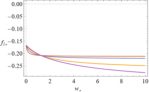

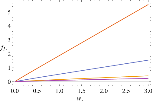
Extending the polynomial truncation does not generate new non-trivial values for the fixed-point couplings:
| (V.7) |
Thus, the higher-order couplings do not alter the previous conclusions. In particular, for all fixed points, the value of remains independent of and . Moreover, apart from the special case in which , the fixed-point value of is the same in all cases and is given by
It is therefore defined only for and becomes negative for .
Since the inclusion of running couplings does not modify the scaling solutions in Eqs. (IV.3), (IV.4), and (IV.5), these still provide, within the truncation in Eq. (II.1), exact scaling regimes that can be reached from fully non-trivial running potentials and . By contrast, the running couplings modify the structure of Eq. (IV.4), such that the corresponding scaling regime becomes an isolated point in the space of solutions and cannot be reached from any non-trivial running potential and .
The family structure of the fixed point does not depend on . The fact that qualitative fixed-point physics does not depend on suggests that the corresponding numerical RG trajectories should display the same -independence.
V.2Critical exponents
Replacing the fixed-point values into the critical condition in Eq. (IV.17), we find that only the fixed points in the second class can satisfy it. Since we require , only the solution with the plus sign in Eq. (LABEL:FPbello) remains. If this fixed point governs the ultraviolet (UV) regime, it can yield asymptotically free solutions for . Whether this happens depends on the spectrum of critical exponents.
We linearize the beta functions around the fixed point by perturbing the running couplings according to
| (V.8) |
where and denotes a critical exponent. For the fixed point eq. (LABEL:FPbello) with the plus sign we find a set of critical exponents that contains the canonical values , , and , as well as two additional non-trivial exponents, denoted by and , which depend on . Figures 4 and 4 show and as functions of for representative values of . The exponent is always positive and typically of order . By contrast, crosses zero at a value . For instance, for one finds for . In the following we focus on the parameter region , for which both non-trivial exponents are positive and the fixed point is UV-attractive in all directions relevant for the UV completion mechanism discussed in Sec. IV.


Inspecting the corresponding eigenvectors, the exponent is associated with the direction, whereas the remaining eigendirections are non-trivial superpositions in the subspace. Nevertheless, their projections show that the most relevant deformation has a dominant component along the Newton coupling . This indicates that the UV scaling regime is largely controlled by the gravitational sector. The marginal and near-marginal eigendirections are also dominated by the gravitational sector but with subleading admixtures of and . In particular, the fixed point breaks the classical marginality of and renders it relevant:
| (V.9) |
where and are two free coefficients. At linear order, is marginal in the fixed-point regime; beyond linear order it acquires logarithmic corrections, corresponding to a marginally (ir)relevant behavior:
| (V.10) |
where , and are complicated numbers depending on and .
In the parameter region , the fixed point is UV-attractive in the sense required for the UV completion mechanism described above. Since the existence of the plus-sign fixed point requires , the singularity can be removed only for an multiplet with at least two scalar fields.
From the beta functions in Appendix B, the anomalous dimension also contributes to the breaking of classical marginality. However, our qualitative conclusions do not hinge on these contributions: setting leaves the fixed-point mechanism and the associated relevance properties unchanged. The breaking of marginality is thus a genuine feature of the fixed point.
Extending the polynomial truncation in Eq. (LABEL:truncpol) does not modify the physical structure of the UV critical manifold. Its only effect is to introduce additional irrelevant directions with , while the non-trivial critical exponents and approach their exact values in the limit . The general properties of the UV critical manifold, derived from perturbations of the scaling solutions in Eq. (IV.5), as well as their relation to polynomial truncations around the minimum, are discussed in more detail in Appendix C. There, we also present the general formula for the critical exponents and show explicitly that they are independent of the regulator parameters and .
The RG flow on the UV critical surface spanned by the UV fixed point yields definite predictions for the infrared (IR) values of couplings at a reference scale . In practice, the projection of the UV critical surface onto the IR hyperplane spanned by partitions the space of IR initial conditions into two regions, which we denote by and . Initial conditions in correspond to trajectories that remain regular for all scales and are attracted to the UV fixed point: for these trajectories gravitational fluctuations overcome matter fluctuations around the Planck scale and the conditions in Sec. IV are satisfied, yielding UV-complete theories. By contrast, initial conditions in lie outside the basin of attraction of the UV fixed point: matter fluctuations continue to dominate above the Planck scale, the conditions in Eq. (IV.17) and are not met, and the flow develops a Landau-pole-like singularity in the UV. Accordingly, points in correspond to trajectories that cannot be connected to the UV fixed point.
Since matter fluctuations dominate in the deep IR, following UV-complete trajectories towards typically brings them close to the Gaussian regime, where the couplings run according to their canonical scaling. However, reaching the Gaussian fixed point itself requires a tuning of the IR-relevant directions. In particular, the running of the minimum generally includes contributions such as , reflecting the presence of relevant directions around the Gaussian fixed point. As a consequence, there exists a continuous family of RG trajectories approaching the Gaussian regime, while only a subset of them reaches the Gaussian fixed point exactly.
VI Numerical analysis to determine the critical line
Determining the manifolds and requires a numerical analysis. As in the fixed-point discussion, we use for illustration. We solve the coupled beta functions for the running couplings given in Appendix B, at fixed and . As boundary conditions we specify the couplings at , corresponding to , i.e. the reference scale at which the IR parameters are defined, and integrate towards increasing RG time (towards the UV).
Trajectories that develop a singularity (belonging to ) terminate at a finite RG time , defined operationally as the smallest value of at which the flow becomes singular (e.g. by a divergence of a coupling or by a vanishing denominator in the beta functions). This induces a separating surface in the space of initial conditions, which we may schematically represent as
| (VI.1) |
where encodes the condition that a singularity is reached at . In the purely scalar limit one recovers the standard one-loop behavior , which implies a divergence at a finite for and reduces to with . For , the existence of the UV-attractive fixed point discussed in Sec. V implies that there are initial conditions for which remains regular for all and flows to . Accordingly, the set of initial conditions that develop a singularity forms a bounded region in the coupling space, separated from the regular region by a critical surface.
To visualize this critical surface, we fix and explore the plane of initial conditions . In this two-dimensional slice, the separating surface reduces to a critical line, which we parametrize as
| (VI.2) |
We then repeat this analysis by varying , , and one at a time, and subsequently scanning also over and .
To avoid numerical instabilities close to the divergence in RG time, we reparametrize the flow by using as the evolution parameter. Concretely, we form ratios such as
| (VI.3) |
and solve the resulting system with initial conditions , , , . For a fixed value of we then scan over and determine whether the solution reaches at finite or instead remains regular and flows towards the UV fixed point. The critical value is identified as the boundary between these behaviors. Repeating this procedure for a range of yields the full curve . The region enclosed by this curve corresponds to the initial conditions for which becomes asymptotically free in the UV; it is the projection of onto the plane at fixed . An example of such a projection is shown in Fig. 7.
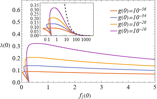
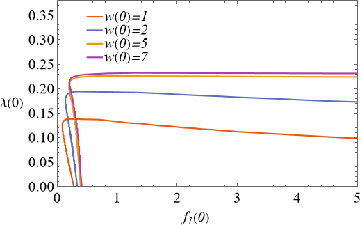
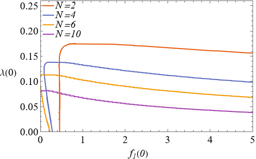
In our analysis we find that the value of has no appreciable impact on the critical line . Figure 7 shows for , , and several values of chosen near the Gaussian regime . The curves exhibit a single maximum and decay to as . As increases, the maximum shifts to larger values of . A similar behavior is observed when fixing and varying : Fig. 7 shows the critical line for different values of at fixed and . Varying the number of scalar fields also yields a similar qualitative behavior, as shown in Fig. 7.
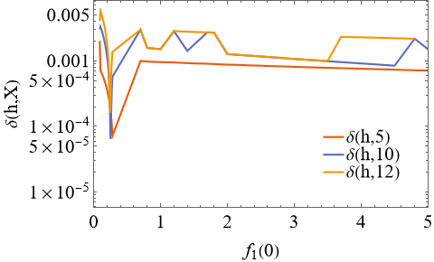
Finally, varying the cutoff-shape parameter at fixed initial conditions and fixed , we find only a mild dependence of the critical line on . This is illustrated in Fig. 7, which shows the logarithm of the absolute difference
| (VI.4) |
for several values as a function of (with ). This indicates that the existence and qualitative shape of the critical line are not artifacts of the parameter .
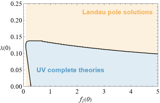
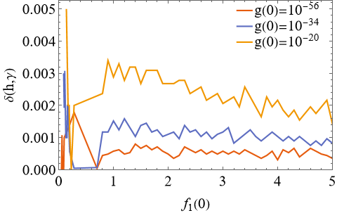
The same analysis can be performed for the second cutoff family . For identical initial conditions and the same values of and , we find that the critical line is insensitive to the choice of . This is shown in Fig. 7, where we plot
| (VI.5) |
as a function of for several values of . We therefore conclude that the critical line is not an artifact of the cutoff family.
In all plots the critical line starts at a minimum value for which . This threshold depends only on and . For slightly above , the critical line rises approximately linearly in , with a slope that depends on . After reaching a maximum, the curve enters an asymptotic regime in which it decays as
| (VI.6) |
in this regime there is no dependence on the initial conditions of , and . Additionally, there is also no dependence on since , so the critical line is cutoff independent for . Also, in this limit, at fixed , all critical lines focus into a single line, this is shown in the inset of fig. 7.
Now we briefly recast the previous results in geometric terms, which also clarifies the origin of the asymptotic relation eq. (VI.6). The RG flow defines a vector field on the coupling space,
| (VI.7) |
whose integral curves are the RG trajectories. Let denote the UV fixed point in eq.(LABEL:FPbello) (with the plus sign). The set of initial data at whose trajectories are regular for all and satisfy defines the IR UV-complete manifold . Equivalently, is the intersection at of the (UV) stable manifold of the fixed point with the IR hyperplane.
Locally, can be described as the zero level-set of a function ,
| (VI.8) |
and the defining property of such an invariant manifold is that the RG vector field is tangent to it. Denoting by the normal to the hypersurface, tangency is expressed by
| (VI.9) |
Selecting as a representative coupling, one may equivalently parameterize the manifold as
| (VI.10) |
so that eq. (VI.9) becomes a first-order condition determining along the RG characteristics.
In the large- regime at fixed , the UV-complete trajectories rapidly approach the fixed-point values of the remaining couplings, , while acts as an external large parameter in the projection to the plane. To leading order, the tangency condition eq. (VI.9) therefore reduces to the requirement that the -component of the flow vanishes on the asymptotic trajectory 111In eq. (VI.11) the coupling is replaced by and not simply by due to the Taylor expansion of .,
| (VI.11) |
Solving this equation for and expanding for yields precisely the asymptotic critical line eq. (VI.6), explaining why, at fixed , the numerical critical lines collapse onto a single curve in that limit (cf. the inset of Fig. 7).
VII Numerical solutions
VII.1Numerical runnings
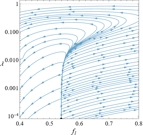
The flow equations in Appendix B can be solved only numerically. Eliminating from the solutions, one can construct RG trajectories in the five-dimensional coupling space or equivalently the hypersurface . Since these trajectories cannot be visualized in the full space, we show representative projections of . In particular, the projection onto the plane for scales above the Planck regime is shown in Fig. 9. For initial conditions inside the UV-complete region (the projection of in Fig. 7), all trajectories approach the interacting UV fixed point.
Before presenting the numerical runnings, it is useful to describe how to fix the boundary conditions at , especially for the Newtonian constant and for the minimum of the potential. In the IR region at we require that
| (VII.1) |
where is the Plank mass: . In terms of adimensional Newtonian constant, this translates to
| (VII.2) |
In the IR (namely, for the solutions where ), gravitational fluctuations should decouple from the dynamics and this restricts to lie in the Gaussian regime so that the relation
| (VII.3) |
has to be satisfied to have a well-defined decoupling regime in which gravitational fluctuations do not dominate the infrared dynamics. In this regime, infrared observables are expected not to exhibit large hierarchies induced by the ultraviolet scale. In particular, this suggests that the IR value of is of order one. We therefore choose the representative value
| (VII.4) |
that is, the vacuum expectation value should be of the same order as the measurement scale . The condition has to be understood as a representative convenient choice within the natural class of IR configurations that do not exhibit fine-tuning and not as an UV-motivated constraint. In particular, the numerical analysis on the UV complete trajectories shows that the runnings are not affected by the initial condition on so that a unique can be used to describe the runnings.
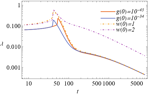
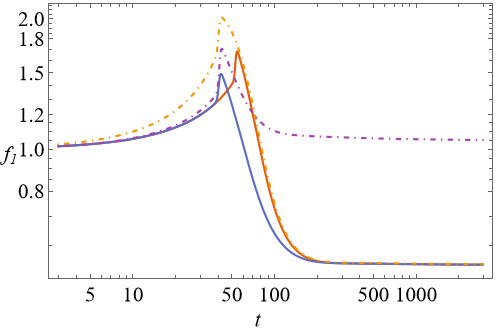
The RG-time evolution of representative UV-complete trajectories for is shown in Figs. 9 and 9. Solid lines correspond to solutions at fixed and for two different values of , namely and . Dot-dashed lines correspond to solutions at fixed and for two different values of , namely and . The running follows the matter-dominated (Gaussian) behavior up to a transition value
| (VII.5) |
at which gravitational fluctuations become important and crosses over from the Gaussian regime to the non-Gaussian fixed-point regime. Around this crossover, reaches a maximum and subsequently decreases towards , with an asymptotic behavior compatible with at large . The running of shows a similar crossover and approaches its fixed-point value in the UV.
The transition scale is where the critical condition eq.(IV.17) starts to be satisfied. Indeed, the maximum of corresponds to a zero of the beta function . This is exactly where the condition of Sec. IV holds and then for larger the inequality is satisfied, allowing the decreasing of . In particular, in the limit eq.(IV.17) gives the constraint , which eq.(LABEL:FPbello) satisfies, and the running of and reduces to and reproducing the exact scaling solution.
In all cases, the running of shown in Fig. 12 is qualitatively similar to the pure-gravity behavior: a Gaussian regime at low scales crosses over to the non-Gaussian scaling regime around . The running of , shown in Fig. 12, exhibits two quasi-constant regimes; the second is approached in the non-Gaussian fixed-point regime of Eq. (LABEL:FPbello). In particular, the system remains in the symmetry-broken phase along the displayed trajectories.
Figures 12 and 12 show the anomalous dimensions and . Both remain small but non-vanishing. As for , they develop a peak around the crossover to the non-Gaussian regime and then decay slowly towards their fixed-point values and . Due to the smallness of , the ratio in Figs. 12 and 12 is nearly constant over the full RG interval. Deviations from the IR value start around , after which approaches its UV value. The initial conditions thus fix the free parameter of the UV fixed point eq. (LABEL:FPbello), which in turn determines the corresponding fixed-point values and .


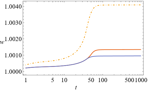
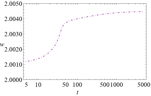
Changing at fixed and primarily affects the length of the matter-dominated regime: the smaller is, the longer the trajectory stays close to the Gaussian regime before crossing over. The location of the maximum in and shifts accordingly, while the UV scaling behavior is essentially unchanged. By contrast, changing at fixed and mainly affects the UV scaling regime and its approach to the fixed point. While depends only weakly on , the maxima of and , as well as the asymptotic coefficients in the large- expansions (e.g. ), show a pronounced dependence on . This is reflected in the different numerical values of and approached in the UV.
VII.2Limits on the mass of the scalar
The independence of the critical line from and allows us to extract predictions that are insensitive to the cutoff choice. In particular, it can be used to constrain the scalar mass in the broken phase, cf. Eq. (II.15), evaluated at the reference scale .
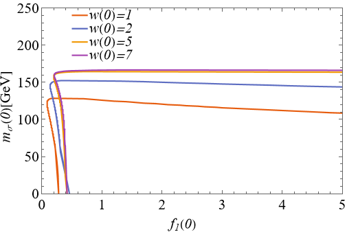
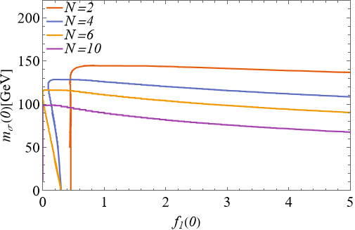
Figure 14 illustrates how the projection of the IR critical manifold constrains the scalar mass at fixed , and . In this representation, the critical line in the plane becomes a critical mass line in the plane: as in the previous discussion, the region below the curve corresponds to UV-complete trajectories, while points above it lead to Landau-pole-like behavior. The critical mass line exhibits a maximum and then decreases at large . In the asymptotic limit , using eq.(VI.6) we get
| (VII.6) |
replacing the fixed point value shows that this expression does not depend on , as for the asymptotic of the critical line. Furthermore, in this asymptotic limit, all critical mass lines focus on a single critical mass line.
Figure 14 shows the critical mass line as a function of for and several values of . The allowed mass range depends strongly on , changing by many orders of magnitude as is varied. By contrast, at fixed , the dependence on (Fig. 14) and on (Fig. 14) is milder, and the resulting mass range typically remains within the same order of magnitude.

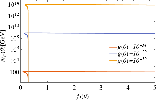
The maximum allowed scalar mass is determined by the peak of the critical line, i.e. by the pair with . In , at , one finds
| (VII.7) |
This expression makes the strong sensitivity to explicit. Expanding around yields . Since , the overall scale is set by the competition between the largeness of and the smallness of . If is not small enough to compensate the Planck scale, the maximum scalar mass remains parametrically below ; conversely, for extremely small the maximum mass becomes very small. For example, for (corresponding to a measurement performed at ) we find but with (corresponding to ) we find .
As a further illustrative example, consider and a reference scale near the top-quark mass, , for which . In this case we find , which along with the condition gives and then corresponds to .
Following the UV complete trajectories from the UV scaling regime () to the IR () can produce scalar masses both much larger and much smaller than the Planck mass, depending on how the parameters in the UV critical manifold evolve in the IR. This happens because although for , gravitational fluctuations decouple, so that infrared observables are not driven by the ultraviolet scale and do not develop UV-induced hierarchies, this does not preclude hierarchies that originate from the choice of UV data along relevant directions. In particular, the constraint remains sensitive to the UV initial conditions. Accordingly, achieving scalar masses in the IR much smaller than the Planck scale while simultaneously matching generally requires a degree of fine-tuning in the UV initial conditions. In contrast, the choice does not follow from the dynamics but represents a convenient IR reference value within the class .
VII.3Running of the scalar mass

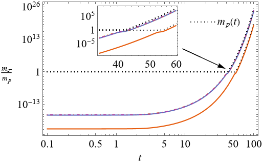
We now discuss the running of the longitudinal scalar mass. Figure 15 shows the RG evolution of the dimensionless mass for the four numerical solutions introduced in Sec. VII.1. For the running is almost frozen, . Around the transition scale , where gravitational fluctuations start to dominate, develops a maximum and then crosses a short transient regime before approaching the UV fixed point value .
In the asymptotic UV regime we find a slow decay,
| (VII.8) |
This behavior is expected: near the UV fixed point all couplings approach constant values, while the quartic coupling is marginally running as . Since at leading order (cf. Eq. (II.15)), one obtains .
The dependence on the IR initial conditions mirrors the behavior discussed for in Sec. VII.1: changing at fixed mainly shifts the extent of the matter-dominated regime below , whereas changing at fixed primarily affects the gravity-dominated regime above .
Figure 15 shows the corresponding dimensionful mass, plotted in units of the reference Planck mass at . Below the nearly constant implies the canonical scaling . Above the UV decay of induces an additional suppression, so that
| (VII.9) |
In the same figure we also show the running Planck mass (dotted curves). In the matter-dominated regime is approximately constant, while above it follows the same overall scaling pattern as . This can be understood from the critical relation eq. (IV.17), which becomes approximately saturated above the transition and implies . Inserting this into Eq. (II.15) yields the parametric estimate
| (VII.10) |
showing that is of order up to a factor , and hence as in the UV.
VII.4The numerical runnings in the deep IR regime
The numerical integration can also be extended to , corresponding to the deep infrared (IR) regime. In this region, gravitational fluctuations effectively decouple, and the running of the couplings becomes insensitive to . The dynamics is then entirely driven by matter fluctuations. In particular, the flows of , and decouple from the flow of , so that is fully determined by the running of , and . For fixed initial conditions on , the residual dependence of the flow is controlled by the choice of .
In order to display the infrared behavior in a log-log representation, we redefine the RG time as , such that the deep IR limit corresponds to . This reparametrization is introduced purely for visualization purposes.
Figs. 18 and 18 show the numerical running of and for , corresponding to the solutions with and shown in Figs. 9 and 9. Both couplings decrease and approach asymptotic values in the deep IR (), with limiting values that depend on .
In the deep IR, the running minimum enters the Gaussian regime and exhibits canonical scaling, (Fig. 18). Similarly, the dimensionless scalar mass scales as (Fig. 18). This corresponds to the system flowing into the spontaneously broken phase, where the dimensionful vacuum expectation value approaches a constant. In contrast to the running of and , the solutions show no visible dependence on the initial value : the corresponding trajectories are numerically indistinguishable within the resolution of the plots.
The behavior of the anomalous dimensions in the deep IR clarifies the effective dynamics of the model. The longitudinal anomalous dimension (Fig. 18) vanishes for , while the transverse anomalous dimension approaches (Fig. 18). Accordingly, the wavefunction renormalizations scale as and . In this regime, the longitudinal (radial) mode decouples from the flow, and the dynamics is dominated by the transverse (Goldstone) modes. As a result, the effective IR theory is governed by Goldstone fluctuations and is equivalent to a non-linear sigma model at scales . This behavior is well established within the functional renormalization group framework for models [11, 40, 38, 121].
The dominance of Goldstone modes is also reflected in the behavior of (inset of Fig. 18), which in the deep IR scales as
| (VII.11) |
indicating that .
The behavior should not be interpreted as a physical anomalous dimension, but rather as a consequence of the strong running of the wavefunction renormalization within the present truncation. In particular, the scaling implies that the combination approaches a constant, consistently with the emergence of Goldstone dynamics in the infrared. In more refined treatments, the anomalous dimension of Goldstone modes is known to remain small, so should be regarded as a truncation artifact [40, 38].
Although the dimensionless couplings and approach constant values in the deep IR, this does not correspond to a finite interaction strength for canonically normalized Goldstone fields. Due to the strong running of the transverse wavefunction renormalization , the corresponding physical interactions are suppressed in the infrared.


VIII Conclusions
In this work we studied an scalar theory non-minimally coupled to Einstein gravity in the symmetry-broken phase. Using a polynomial truncation around the running minimum of the scalar potential, we employed the proper-time flow equation to compute the RG running of the minimum of the potential, the non-minimal coupling, the quartic coupling, and the cosmological-constant term within the truncation.
Working with the exponential parametrization and the physical gauge, we identified an interacting UV-attractive fixed point. This fixed point opens the possibility of UV-complete trajectories for the quartic scalar coupling without invoking fermionic degrees of freedom. The fixed point is associated with a scaling solution of the underlying flow equation of the form and . Within the truncation scheme for the derivative expansion adopted in this work, this scaling solution is realized exactly at the fixed point and is not affected by the order of the polynomial expansion around the running minimum, as well as on the cutoff parameter . As shown in Appendix C, these properties follow from an analysis of the linearized flow around the scaling solution, which does not rely on a finite polynomial truncation. In particular, this perturbative analysis leads to a consistent determination of the UV critical manifold. This independence from the polynomial truncation and provides non-trivial evidence for the robustness of the corresponding UV scaling regime, although a full assessment of truncation effects would require more refined approximations.
The fixed-point value of lies close to the conformal value, with determined by Eq. (LABEL:FPbello). Closely related fixed-point structures in scalar–tensor systems have also been reported within the Wetterich formalism, see e.g. [77].
The UV fixed point spans a finite-dimensional UV critical surface. Its stability spectrum contains the canonical exponents , and , as well as additional non-trivial exponents that depend on and on the free fixed-point parameter (see Figs. 4 and 4). The associated eigendirections are, in general, non-trivial superpositions in the space of couplings. Apart from the direction associated with (with ), the most relevant deformation has a dominant projection along the Newton coupling . This indicates that the approach to the UV fixed point is largely controlled by gravitational fluctuations. In particular, the fixed point breaks the classical marginality of and renders it relevant, while is marginal at linear order and acquires logarithmic corrections beyond linear order, consistent with an asymptotic behavior of the form .
Evolving trajectories on the UV critical surface towards the infrared defines a corresponding basin of attraction in the space of IR couplings. This basin contains precisely those IR initial conditions that lead to UV-complete trajectories attracted to the UV fixed point. In practice, this separates IR initial data into two classes: one class yields regular flows for all scales and approaches the UV fixed point, while the complementary class develops a singularity at finite . The separating boundary can be characterized numerically and, at fixed , appears as a critical line in the plane (see Fig. 7). We find that this critical line is robust under changes of the cutoff family (switching between and ) and depends only mildly on the cutoff-shape parameter . Its dependence on is also weak, while the strongest dependence is on , and , in line with the fact that the UV scaling regime is strongly influenced by the -direction.
The critical line provides a practical UV-completion criterion: for given , UV-complete trajectories correspond to IR values lying in the region bounded by . Adopting the naturalness-motivated choice allows us to translate this constraint into bounds on the physical mass of the longitudinal mode via Eq. (II.15). Interestingly enough, the peak of the critical line determines an upper bound for fixed and . For illustrative choices of in the vicinity of the electroweak scale, the resulting upper bounds can lie in the range.
In the deep infrared (), the flow exhibits the characteristic features of the spontaneously broken phase: the radial mode becomes effectively decoupled, while the transverse Goldstone modes dominate the dynamics. In this regime, the effective theory is well described by a non-linear sigma model, with the radial fluctuations frozen out and the dynamics constrained to the vacuum manifold.
An important next step is to extend the present framework to more realistic matter sectors. Including gauge fields and fermions introduces additional fluctuation channels that feed into the running of the scalar potential and of the non-minimal coupling. In particular, gravitational fluctuations are known to favor antiscreening contributions in Abelian gauge sectors, suggesting that the mechanism identified here may persist in the presence of gauge interactions and could potentially be relevant for curing Landau-pole behavior in Abelian theories. At the same time, Yukawa interactions provide a competing contribution to the scalar self-coupling and can shift the UV behavior of . It will therefore be important to determine whether the UV-attractive fixed point characterized here by and survives once gauge and Yukawa couplings are included, and to map the resulting UV-complete region in the enlarged theory space.
The present analysis is formulated within a Wilsonian renormalization group framework based on a proper-time flow equation. In this setting, the proper-time construction can be interpreted as defining a consistent Wilsonian flow associated with a specific coarse-graining prescription. At the same time, closely related structures are expected to arise within the Wetterich formulation of the functional renormalization group for the effective average action. In comparable truncations and for consistent choices of gauge and field parametrization, both approaches are known to exhibit similar fixed-point structures. For this reason, it will be important to repeat and cross-check the present analysis within an exact EAA/Wetterich framework, in order to further assess the robustness of the results.
Acknowledgements
We thank Andrea Spina Gabriele Giacometti for useful discussions, and Dario Zappalà and Giampaolo Vacca for comments on the manuscript. A.B. is grateful to Holger Gies for enlightening discussions on and to the Physics Department of the University of Jena for hospitality.
Appendix A Derivation of the flow equations for and
In this appendix we derive the proper-time flow equations for the running wave-function renormalizations and entering Eq. (II.1). We build on the background-field and heat-kernel setup of Ref. [18].
A.1Projection on the kinetic operators
To extract and we project the flow on the operators () and , respectively. Since we are projecting on the scalar kinetic terms, only the scalar block of the Hessian is required. The projection reads
| (A.1) |
where denotes the scalar block of the Hessian, the corresponding matrix of kinetic prefactors, and includes the functional trace and the internal trace.
The scalar Hessian can be written as (see Ref. [18])
| (A.2) |
with
| (A.3) |
and
| (A.4) |
Here a bar denotes evaluation on the background, and and are the longitudinal (radial) and transverse projectors defined in the main text.
It is convenient to introduce the longitudinal and transverse “mass” terms
| (A.5) |
with
| (A.6) |
A.2Heat-kernel expansion
We bring the operator to Laplace type by factoring out ,
| (A.7) |
In components, decomposes as
| (A.8) |
the term and correspond to the physical longitudinal and Goldstone mass mode, respectively.
For later reference, in a flat background () and evaluated at the running minimum , the transverse mass vanishes (Goldstone modes), while the longitudinal one reduces to the mass term used in Eq. (II.15) after conversion to dimensionless variables. In what follows we set , since and are extracted from the scalar kinetic terms and we focus on the flat-background projection.
The functional trace is evaluated using the early-time heat-kernel expansion for a Laplace-type operator ,
| (A.9) |
with (see e.g. [7, 9, 8, 6, 4])
| (A.10) |
Here denotes the internal trace only. The -functionals are Mellin transforms,
| (A.11) |
where in our case, from eq.(A.1), we read .
Since we work on a background without boundary (and ultimately set ), total derivatives can be dropped. In particular, the contribution is a total derivative, and in we may use to trade the term for up to total derivatives. Thus, for the kinetic projection it is sufficient to keep the structure.
A.3Derivative structure and separation into longitudinal/transverse sectors
We compute
| (A.12) |
Using and that are functions of , one finds
| (A.13) |
The required projector identities are
| (A.14) |
and
| (A.15) |
Therefore,
| (A.16) |
We now evaluate on an -breaking background pointing in the -direction, so that only the longitudinal background component is nonzero. In this case projects onto the longitudinal fluctuation sector, while the transverse sector is isolated by the term proportional to . Explicitly, after evaluating on the background,
| (A.17) |
with
| (A.18) |
A.4Proper-time integrals and flows of and
Keeping only the term in Eq. (A.9) and inserting Eq. (A.17) into the flow, we obtain
| (A.19) |
where
| (A.20) |
Matching to the left-hand side of Eq. (A.1) yields
| (A.21) |
Using the cutoff kernel in Eq. (I.2) (type-C: ) one may perform the -integral in and then the -integral. A convenient identity is
| (A.22) |
which is to be used with , (longitudinal) or , (transverse), and for the present projection.
A.5Consistency check: the limit
It is instructive to verify how the case is recovered. In Eq. (LABEL:dU2final), the transverse contribution is proportional to
For , and , hence
| (A.25) |
Therefore only the longitudinal contribution remains, as expected.
Appendix B The beta functions
In this appendix we derive the beta functions for the ansats
| (B.1) |
The beta functions can be found replacing the ansats in eqs.(LABEL:adeqfull) and expanding in series around .
In the flow equation for is given by
| (B.2) |
The flow equation for is given by
| (B.3) |
The flow equation for is given by
| (B.4) |
where
| (B.5) |
The flow equation for is given by
| (B.6) |
The flow equation of is given by
| (B.7) |
All beta functions do not depend on , consequently the equations are decoupled with respect to the flow of . In the flow equations, the quantity is the dimensionless longitudinal scalar mass. The flow equations do not depend on and the presence of appears only by . The presence of breaks the classical marginality of , and shifts the classical scaling of . The flow of can be written in the standard form . The gravitational anomalous dimension does not depend on and whereas appears only by the presence of the longitudinal scalar mass.
In the full flow equations eqs.(LABEL:adeqfull) the potential is coupled to gravity only by . In term of ansats eq.(LABEL:ansappbeta), this translates in the flow of coupled to the newtonian constant only by . This is a feature of the physical gauge. The origin of this can be found writing the pysical gauge in terms of background field gauge method. With the standard notation of [105], the physical gauge is the limit and . In the flow equations for general and the newtonian constant always appears in the form [105]. Accordingly, in the limit the standard terms disappear and is coupled to the potential only if the newtonian constant has a field dependence.
The flow equation for is given by
| (B.8) |
The equation for and can be derived simply replacing the ansatz in eq.(II.12) and putting . The results are
| (B.9) |
In this way the flow equation of is given by
| (B.10) |
from eq.(LABEL:betaetaL) we see that at the fixed point the two anomalous dimensions vanish, so is a free parameter.
Appendix C Perturbations of the scaling solution and
In this appendix, we derive the perturbations to the exact scaling solution and of eq.(LABEL:adeqfull), which have not been discussed in [18]. The following discussion shed light on properties of the UV complete solutions we discussed in the main text but also give a more general insight far from the minimum of the potential.
The values of the coefficients and of the exact scaling solution are given in eq.(LABEL:FPbello). We consider the perturbations of the solution with the plus sign, which yields the UV complete solutions discussed in the text.
Before proceeding, we emphasize that the scaling solution , is defined only for . At , the gravitational coupling vanishes, which invalidates the ansatz . In fact, the configuration , does not satisfy the fixed-point version of Eq. (LABEL:adeqfull)222The fixed-point version of Eq. (LABEL:adeqfull) with the ansatz and is satisfied only for . However, this value is pathological, as it corresponds to a negative Newton constant.. This implies that a polynomial expansion around for the solutions of Eq. (LABEL:adeqfull) does not admit a fixed point that reconstructs in the UV limit (). This is in contrast to the expansion around , where Eq. (LABEL:FPbello) yields , which is equivalent to the lower bound of the critical condition in Eq. (IV.17). As a consequence, in the symmetric phase there is no UV-complete solution exhibiting the scaling regime , . In particular, the removal of the Landau pole in the symmetric phase cannot be achieved within a simple truncation of the form , as Eq. (LABEL:adeqfull) does not admit a scaling solution capable of realizing this behavior. In this case, additional fields, interactions, or extensions of the derivative expansion are required.
The general perturbations of the scaling solution can be written as
| (C.1) |
replacing them in the flow equations and expanding around at the linear order we get
| (C.2) |
where
| (C.3) |
and
| (C.4) |
The mixing coefficients are given by
| (C.5) |
The perturbations for and are two second order linear partial differential equations. In particular, the equation for is a homogeneous equation decoupled from , whereas the equation for is a non-homogeneous equation . The perturbation for is a free parameter. This is due to the perturbations of the anomalous dimensions, which are always of the second order in the perturbative expansion.
The equation for can be solved exactly. A solution can be found with the method of the separation of variables with ansats where is the separation constant, which describes the critical exponents of the solution. The function then satisfies a linear second order differential equation whose solution is given by
| (C.6) |
where is the Tricomi confluent hypergeometric function, are the generalized Laguerre polynomial and , are two free parameters. The general solution is a superposition of .
The equation for has a general solution that can always be written as
| (C.7) |
where solves the homogeneous equation and is a particular solution. The homogeneous solution can be found again with the method of separation of variables with an ansats . The separation constant does not necessarily coincide with as the differential equations of and are decoupled. The dependent part of the homogeneous solution is given by
| (C.8) |
where
| (C.9) |
The particular solution is given formally by
| (C.10) |
where is the Green function of the differential operator . Due to the complexity of the Green function, the particular solution can be found only numerically, except in the asymptotics or locally around some point .
The critical properties of the theory depend only on the homogeneous solution. In order to obtain well-defined critical exponents, we have to require that both branches of the solution are regular over the entire range of , from zero to infinity. While the Laguerre polynomials are smooth functions, the Tricomi confluent hypergeometric function , with argument , exhibits a singular behavior around :
| (C.11) |
If , this leads to a singularity at . In order to avoid this singular behavior, must also be singular, which occurs when , with .
Beyond regularity, one must also require that the solution does not exhibit exponential growth at large . In the asymptotic limit , the Tricomi function yields a power-law behavior, whereas the generalized Laguerre polynomial behaves as
| (C.12) |
Therefore, in order to eliminate the exponential term, the condition or must be satisfied.
In Eqs. (C.6) and (LABEL:solpertf), the parameter of the generalized Laguerre polynomial is equal in magnitude but opposite in sign to that of the Tricomi function. As a result, imposing the condition simultaneously removes both the singularity at the origin and the exponential growth at infinity.
In our case, for fixed and , both appearing in and have . Therefore, imposing to remove the divergences at and the exponential behavior at uniquely fixes the critical exponents. In particular, this leads to two independent sets of critical exponents.
From Eq. (C.6) we obtain
| (C.13) |
This result does not depend on or on the regulator parameter . The values and correspond to relevant directions, yields a marginal direction, and correspond to irrelevant directions. This explains the origin of the integer critical exponents associated with the UV-complete solutions discussed in Sec. V.
More generally, repeating the analysis of Sec. V with a truncation of the form
and comparing with Eq. (C.13) shows that the renormalizable couplings and are associated with the directions and , respectively, while the higher-order couplings , , …correspond to irrelevant directions. The value is instead associated with the scalar mass generated by the non-trivial potential.
Replacing eq.(C.13) in the pertubation , eq.(C.6), turns the solution into a simple polynomial of degree . The general solution for is given by
| (C.14) |
where
| (C.15) |
the coefficients are complicated and long functions of and , which we do not show explicitly.
From eq.(LABEL:solpertf) we get
| (C.16) |
where
| (C.17) |
This result does not depend on the regulator parameter , but it does depend on and . The number of relevant directions is given by , where is defined as , with given in Eq. (LABEL:critexpf). By plotting as a function of for different values of , we find for and for . Consequently, for and for . This matches the number of non-trivial critical exponents found in Sec. V. In particular, the values are very close to those shown in Figs. 4 and 4. For example, for and , we obtain () and (), while the corresponding values extracted from the plots are and . The small discrepancy between these results is due to truncation effects. Repeating the analysis of Sec. V with higher-order truncations in the expansion of around , the values and converge toward and . This explains the origin of the two non-trivial critical exponents associated with the UV-complete solutions.
As for , replacing eq.(LABEL:critexpf) in the pertubation , eq.(LABEL:solpertf), turns the solution into a simple polynomial of degree . The general homogeneous solution for is given by
| (C.18) |
where
| (C.19) |
the coefficients are complicated and long functions of and , which we do not show explicitly.
Replacing eq.(C.14) in the perturbation equation of and expanding around with a Frobenius ansats for , we find that the particular solution in this regime can be written as
| (C.20) |
for all , where the coefficients are a linear combination of for :
| (C.21) |
the coefficients are long and complicated functions of , and that we do not show explicitly. The relevant direction does not appear because this yields a constant eigenfunction and in eq.(LABEL:eqpertuf) only derivatives of appear.
The particular solution for is always a smooth function around the origin. A similar conclusion holds for an expansion around a generic where we find
| (C.22) |
where the coefficients have the same structure as . A particular case arises when coincides with the running minimum of the potential. In this case, acquires an explicit -dependence and the resulting solution is modified. This situation will be analyzed in the following.
A different situation arises in the asymptotic regime , where the leading order of the Frobenius ansatz depends on the largest included in the expansion. Truncating the series in Eq. (C.14) at , the particular solution in this regime can be written as
| (C.23) |
Here,
| (C.24) |
so that the coefficients consist of superpositions of exponential terms , together with contributions linear in multiplied by the same exponential factors.
Fixing and , the exponent of the overall coefficient
in eq.(LABEL:solpertf) always lies in the interval . Accordingly, the perturbation diverges as , even though the singularities of the Tricomi functions have been removed. The only way to cancel this divergence is to impose the condition
However, it is important to stress that the behavior at does not affect the physical interpretation of the solutions. As discussed at the beginning of this appendix, a divergence at for is in fact expected on general grounds. At , the scaling solution reduces to , which does not admit a physical interpretation, since the effective Newton coupling becomes ill-defined. Accordingly, the parametrization in terms of breaks down at , and perturbations around this point are not expected to be well-defined. From this perspective, the divergence of at is not pathological, but rather signals that this point lies outside the domain where the scaling solution provides a valid description. The physically relevant regime is instead characterized by . In contrast, regularity of the potential at is still required, since admits a well-defined physical interpretation in this limit. The different behavior of and therefore reflects the fact that the truncation treats the scalar potential and the gravitational coupling in parametrizations with distinct domains of validity.
The solution for in eq.(C.14) can be used to clarify the origin of the fixed-point value in Eq. (LABEL:FPbello). The marginal solution corresponding to acts as an effective deformation of the scaling solution. Taking the derivative of and setting it to zero reproduces exactly the value of given in Eq. (LABEL:FPbello). Expanding around this value yields the truncation
where and reproduce the fixed-point values in eq.(LABEL:FPbello). Including also the relevant directions with , the minimum is shifted to
| (C.25) |
where is a complicated expression involving the quantities in eq.(C.15). Replacing eq.(C.25) in the solution for in eq.(C.7), the general perturbations around can then be written as
where and are given by
| (C.26) |
where the coefficients are complicated functions involving the quantities in eq.(C.15) and eq.(C.19). Similar expressions can be found by linearizing the flow equations in Appendix B, which have been analyzed in section V.2. This motivates the general ansatz used in the main text.
As a final remark, we note that the linearized flow equations in Appendix B, expanded around the fixed point in Eq. (LABEL:FPbello) and used in Sec. V, are coupled, whereas the perturbative flows derived in this appendix are decoupled. This difference originates from the fact that the expansion around in the full flow equations Eq. (LABEL:adeqfull) retains partial information about the full functional form of , while the present analysis is restricted to perturbations around the scaling solution. Importantly, the critical manifold is determined solely by the perturbations of the scaling solution and is therefore insensitive to the full functional form of . This explains why both approaches yield the same set of critical exponents. However, in the full flow, the perturbations of , , , and related quantities also contain contributions involving superpositions of the non-trivial critical exponents associated with , which are absent in the simplified analysis presented in this appendix.
References
- [1] (2018) Asymptotically safe -gravity coupled to matter I: the polynomial case. Annals Phys. 396, pp. 173–201. External Links: 1802.00498, Document Cited by: §I, §I, §I.
- [2] (1998) Rapidly converging truncation scheme of the exact renormalization group. Prog. Theor. Phys. 99, pp. 451–466. External Links: hep-th/9803056, Document Cited by: §III.
- [3] (2021) Dark matter and the early Universe: a review. Prog. Part. Nucl. Phys. 119, pp. 103865. External Links: 2104.11488, Document Cited by: §I.
- [4] (2000) Heat kernel and quantum gravity. Vol. 64, Springer, New York. External Links: Document, ISBN 978-3-540-67155-8 Cited by: §A.2.
- [5] (2020) Functional renormalization group approach and gauge dependence in gravity theories. Phys. Rev. D 101 (6), pp. 065001. External Links: 1910.06068, Document Cited by: §I, §III.
- [6] (1993-02) Covariant perturbation theory. 4. Third order in the curvature. External Links: 0911.1168 Cited by: §A.2.
- [7] (1990) Covariant perturbation theory. 2: Second order in the curvature. General algorithms. Nucl. Phys. B 333, pp. 471–511. External Links: Document Cited by: §A.2.
- [8] (1990) Covariant perturbation theory. 3: Spectral representations of the third order form-factors. Nucl. Phys. B 333, pp. 512–524. External Links: Document Cited by: §A.2.
- [9] (1987) Beyond the schwinger-dewitt technique: converting loops into trees and in-in currents. Nuclear Physics 282, pp. 163–188. External Links: Link Cited by: §A.2.
- [10] (2010) Taming perturbative divergences in asymptotically safe gravity. Nucl. Phys. B 824, pp. 168–191. External Links: 0902.4630, Document Cited by: §I.
- [11] (2002) Nonperturbative renormalization flow in quantum field theory and statistical physics. Phys. Rept. 363, pp. 223–386. External Links: hep-ph/0005122, Document Cited by: §III, §VII.4.
- [12] (2008) The Standard Model Higgs boson as the inflaton. Phys. Lett. B 659, pp. 703–706. External Links: 0710.3755, Document Cited by: §I.
- [13] (2017) Renormalization group fixed points of foliated gravity-matter systems. JHEP 05, pp. 093. External Links: 1702.06539, Document Cited by: §I, §I.
- [14] (2001) Renormalization group flow equations and the phase transition in O(N) models. Int. J. Mod. Phys. A 16, pp. 3823–3852. External Links: hep-ph/0007098, Document Cited by: §I.
- [15] (2005) Proper time flow equation for gravity. JHEP 02, pp. 035. External Links: hep-th/0410191, Document Cited by: §I.
- [16] (2022) Structural aspects of FRG in quantum tunneling computations. Annals Phys. 445, pp. 169090. External Links: 2206.06917, Document Cited by: §I.
- [17] (2023) The conformal sector of Quantum Einstein Gravity beyond the local potential approximation. Phys. Lett. B 847, pp. 138311. External Links: 2309.15514, Document Cited by: §I.
- [18] (2025-08) Proper-time functional renormalization in scalar models coupled to gravity. External Links: 2508.00807 Cited by: §A.1, Appendix A, Appendix C, §I, §I, §II.2, §III, §IV.1, §IV.1, §IV.1, §IV.1, §IV.1.
- [19] (2012) Universality and Symmetry Breaking in Conformally Reduced Quantum Gravity. Phys. Rev. D 86, pp. 105027. External Links: 1206.6531, Document Cited by: §I.
- [20] (2020) On Exact Proper Time Wilsonian RG Flows. Eur. Phys. J. C 80 (3), pp. 249. External Links: 1912.08135, Document Cited by: §I, §I.
- [21] (2025) Regular black holes from proper-time flow in quantum gravity and their quasinormal modes, shadow and Hawking radiation. JCAP 12, pp. 042. External Links: 2509.12469, Document Cited by: §I.
- [22] (2023) Ultraviolet behavior of conformally reduced quadratic gravity. Phys. Rev. D 108 (2), pp. 026008. External Links: 2304.12011, Document Cited by: §I.
- [23] (2025) Gauge and parametrization dependence of quantum Einstein gravity within the proper time flow. Phys. Rev. D 112 (2), pp. 026002. External Links: 2504.07877, Document Cited by: §I, §I, §I, §III.
- [24] (2001) Towards an accurate determination of the critical exponents with the renormalization group flow equations. Phys. Lett. B 504, pp. 181–187. External Links: hep-th/0010095, Document Cited by: §I.
- [25] (2015) Global solutions of functional fixed point equations via pseudospectral methods. Phys. Rev. D 91 (10), pp. 105011. Note: [Erratum: Phys.Rev.D 93, 089904 (2016)] External Links: 1502.07511, Document Cited by: §II.3.
- [26] (2016) Solving functional flow equations with pseudo-spectral methods. Phys. Rev. D 94, pp. 025027. External Links: 1603.06726, Document Cited by: §II.3.
- [27] (2019-12) Curvature dependence of quantum gravity with scalars. External Links: 1912.01624 Cited by: §I.
- [28] (2013) Investigating the near-criticality of the Higgs boson. JHEP 12, pp. 089. External Links: 1307.3536, Document Cited by: §I.
- [29] (2003) Nonperturbative renormalization group approach to the Ising model: A Derivative expansion at order partial**4. Phys. Rev. B 68, pp. 064421. External Links: hep-th/0302227, Document Cited by: §III.
- [30] (2003) Optimization of the derivative expansion in the nonperturbative renormalization group. Phys. Rev. D 67, pp. 065004. External Links: hep-th/0211055, Document Cited by: §III.
- [31] (2018) Asymptotic safety of gravity with matter. Phys. Rev. D 97 (10), pp. 106012. External Links: 1710.04669, Document Cited by: §I, §I.
- [32] (2024-06) Dark Matter. External Links: 2406.01705 Cited by: §I.
- [33] (2008) Ultraviolet properties of f(R)-gravity. Int. J. Mod. Phys. A 23, pp. 143–150. External Links: 0705.1769, Document Cited by: §I.
- [34] (2009) Investigating the Ultraviolet Properties of Gravity with a Wilsonian Renormalization Group Equation. Annals Phys. 324, pp. 414–469. External Links: 0805.2909, Document Cited by: §I.
- [35] (2018) Exact RG Flow Equations and Quantum Gravity. JHEP 03, pp. 118. External Links: 1707.09298, Document Cited by: §I.
- [36] (2018) Asymptotic safety and field parametrization dependence in the truncation. Phys. Rev. D 98 (2), pp. 026027. External Links: 1805.09656, Document Cited by: §I.
- [37] (2020) Precision calculation of critical exponents in the universality classes with the nonperturbative renormalization group. Phys. Rev. E 101 (4), pp. 042113. External Links: 2001.07525, Document Cited by: §III.
- [38] (2012) An Introduction to the nonperturbative renormalization group. Lect. Notes Phys. 852, pp. 49–132. External Links: cond-mat/0702365, Document Cited by: §VII.4, §VII.4.
- [39] (2014) Matter matters in asymptotically safe quantum gravity. Phys. Rev. D 89 (8), pp. 084035. External Links: 1311.2898, Document Cited by: §I, §I.
- [40] (2021) The nonperturbative functional renormalization group and its applications. Phys. Rept. 910, pp. 1–114. External Links: 2006.04853, Document Cited by: §III, §VII.4, §VII.4.
- [41] (2018) Quantum gravity fluctuations flatten the Planck-scale Higgs potential. Phys. Rev. D 97 (8), pp. 086004. External Links: 1712.00319, Document Cited by: §I.
- [42] (2018) Quantum-gravity predictions for the fine-structure constant. Phys. Lett. B 782, pp. 198–201. External Links: 1711.02949, Document Cited by: §I, §I.
- [43] (2018) Mass difference for charged quarks from asymptotically safe quantum gravity. Phys. Rev. Lett. 121 (15), pp. 151302. External Links: 1803.04027, Document Cited by: §I, §I, §IV.3.
- [44] (2018) Top mass from asymptotic safety. Phys. Lett. B 777, pp. 217–221. External Links: 1707.01107, Document Cited by: §I, §I, §IV.3.
- [45] (2019) Zooming in on fermions and quantum gravity. Phys. Rev. D 99 (8), pp. 086002. External Links: 1812.08782, Document Cited by: §I.
- [46] (2021) Safety in darkness: Higgs portal to simple Yukawa systems. Phys. Lett. B 819, pp. 136455. External Links: 2005.03661, Document Cited by: §I.
- [47] (2019) as the critical dimensionality of asymptotically safe interactions. Phys. Lett. B 793, pp. 383–389. External Links: 1902.06479, Document Cited by: §I.
- [48] (2022-12) Asymptotic safety of gravity with matter. External Links: 2212.07456 Cited by: §I.
- [49] (2018) Upper bound on the Abelian gauge coupling from asymptotic safety. JHEP 01, pp. 030. External Links: 1709.07252, Document Cited by: §I, §I.
- [50] (2019) An asymptotically safe guide to quantum gravity and matter. Front. Astron. Space Sci. 5, pp. 47. External Links: 1810.07615, Document Cited by: §I.
- [51] (2022) Status update: Asymptotically safe gravity-matter systems. Nuovo Cim. C 45 (2), pp. 29. External Links: 2201.11543, Document Cited by: §I.
- [52] (1994) FLow equations for N point functions and bound states. Z. Phys. C 62, pp. 503–510. External Links: hep-ph/9308260, Document Cited by: §I.
- [53] (1998) Gauge dependence of the effective average action in Einstein gravity. Int. J. Mod. Phys. A 13, pp. 607–623. External Links: hep-th/9612019, Document Cited by: §I, §III.
- [54] (2013-01) A bootstrap towards asymptotic safety. External Links: 1301.4191 Cited by: §I.
- [55] (2019) Aspects of asymptotic safety for quantum gravity. Phys. Rev. D 99 (12), pp. 126015. External Links: 1810.08550, Document Cited by: §I.
- [56] (2018) Asymptotic safety of quantum gravity beyond Ricci scalars. Phys. Rev. D 97 (8), pp. 086006. External Links: 1801.00162, Document Cited by: §I.
- [57] (2016) Further evidence for asymptotic safety of quantum gravity. Phys. Rev. D 93 (10), pp. 104022. External Links: 1410.4815, Document Cited by: §I.
- [58] (2016) Renormalization Group Equation for gravity on hyperbolic spaces. Phys. Rev. D 94 (8), pp. 084005. External Links: 1607.08460, Document Cited by: §I.
- [59] (2015) Renormalization of Newton’s constant. Phys. Rev. D 92 (12), pp. 124057. External Links: 1501.05331, Document Cited by: §I, §I.
- [60] (2013) FlowPy: A Numerical solver for functional renormalization group equations. Comput. Phys. Commun. 184, pp. 1931–1945. External Links: 1202.5984, Document Cited by: §II.3.
- [61] (1937) Proper time in classical and quantum mechanics. Phys. Z. Sowjetunion 12, pp. 404–425. Cited by: §I.
- [62] (2025) The quantum criticality of the Standard Model and the hierarchy problem. JHEP 10, pp. 134. External Links: 2506.15919, Document Cited by: §I, §IV.3.
- [63] (2024-10) Spontaneous breaking of diffeomorphism invariance in conformally reduced quantum gravity. External Links: 2410.08916 Cited by: §I.
- [64] (2025-10) On the universal content of the proper time flow in scalar and Yang-Mills theories. External Links: 2510.04896 Cited by: §I, §I.
- [65] (2016) Gravitational Two-Loop Counterterm Is Asymptotically Safe. Phys. Rev. Lett. 116 (21), pp. 211302. External Links: 1601.01800, Document Cited by: §I.
- [66] (2015) Generalized Parametrization Dependence in Quantum Gravity. Phys. Rev. D 92 (8), pp. 084020. External Links: 1507.08859, Document Cited by: §I.
- [67] (2024-10) Proper-time flow equation and non-local truncations in quantum gravity. In 17th Marcel Grossmann Meeting: On Recent Developments in Theoretical and Experimental General Relativity, Gravitation, and Relativistic Field Theories, External Links: 2410.23696 Cited by: §I.
- [68] (2018) Gauge and parametrization ambiguity in quantum gravity. Phys. Rev. D 97 (2), pp. 026015. External Links: 1712.03338, Document Cited by: §I.
- [69] (1986) The ultraviolet behavior of einstein gravity. Nuclear Physics B 266 (3), pp. 709–736. External Links: ISSN 0550-3213, Document, Link Cited by: §I.
- [70] (1981) The Inflationary Universe: A Possible Solution to the Horizon and Flatness Problems. Phys. Rev. D 23, pp. 347–356. External Links: Document Cited by: §I.
- [71] (2020) Scalegenesis and fermionic dark matters in the flatland scenario. Eur. Phys. J. C 80 (5), pp. 368. External Links: 2002.03666, Document Cited by: §I.
- [72] (2017) Asymptotic safety of higher derivative quantum gravity non-minimally coupled with a matter system. JHEP 08, pp. 070. External Links: 1703.09033, Document Cited by: §I, §I, §IV.3.
- [73] (2014) Radiative symmetry breaking at the Fermi scale and flat potential at the Planck scale. Phys. Rev. D 89 (1), pp. 016019. External Links: 1310.4304, Document Cited by: §I.
- [74] (2014) Radiative symmetry breaking from flat potential in various U(1)’ models. Phys. Rev. D 89 (5), pp. 056010. External Links: 1401.5944, Document Cited by: §I.
- [75] (2014) Spacetime curvature and the Higgs stability during inflation. Phys. Rev. Lett. 113 (21), pp. 211102. External Links: 1407.3141, Document Cited by: §I.
- [76] (1993) Scaling exponents in quantum gravity near two-dimensions. Nucl. Phys. B 393, pp. 280–300. External Links: hep-th/9206081, Document Cited by: §I.
- [77] (2016) Asymptotic safety in scalar models coupled to gravity. Phys. Lett. B 753, pp. 274–281. External Links: 1505.05393, Document Cited by: §I, §III, §IV.1, §V.1, §VIII.
- [78] (2013) Dark Energy: A Brief Review. Front. Phys. (Beijing) 8, pp. 828–846. External Links: 1209.0922, Document Cited by: §I.
- [79] (1996) On connection between momentum cutoff and the proper time regularizations. Phys. Rev. D 53, pp. 2020–2036. External Links: hep-th/9501124, Document Cited by: §I.
- [80] (1997) Operator cutoff regularization and renormalization group in Yang-Mills theory. Phys. Rev. D 56, pp. 5008–5033. External Links: hep-th/9511046, Document Cited by: §I.
- [81] (1983) Chaotic Inflation. Phys. Lett. B 129, pp. 177–181. External Links: Document Cited by: §I.
- [82] (2018) Asymptotic safety of scalar field theories. Phys. Rev. D 98 (12), pp. 125006. External Links: 1810.01678, Document Cited by: §I.
- [83] (2011) Ising exponents from the functional renormalisation group. Phys. Rev. D 83, pp. 085009. External Links: 1009.1948, Document Cited by: §I, §III.
- [84] (2001) Derivative expansion and renormalization group flows. JHEP 11, pp. 059. External Links: hep-th/0111159, Document Cited by: §III.
- [85] (2001) Optimized renormalization group flows. Phys. Rev. D 64, pp. 105007. External Links: hep-th/0103195, Document Cited by: §III.
- [86] (2008) On the renormalization group flow of f(R)-gravity. Phys. Rev. D 77, pp. 124045. External Links: 0712.0445, Document Cited by: §I.
- [87] (2001) Proper time regulator and renormalization group flow. Phys. Rev. D 64, pp. 105013. External Links: hep-th/0106230, Document Cited by: §I, §I.
- [88] (2016) Asymptotic safety of gravity-matter systems. Phys. Rev. D 93 (8), pp. 084035. External Links: 1510.07018, Document Cited by: §I, §I.
- [89] (2017) Renormalization group flows and fixed points for a scalar field in curved space with nonminimal coupling. Phys. Rev. D 96 (12), pp. 125007. External Links: 1711.02224, Document Cited by: §I.
- [90] (2001) Convergence of derivative expansions in scalar field theory. Int. J. Mod. Phys. A 16, pp. 2095–2100. External Links: hep-th/0102027, Document Cited by: §III.
- [91] (1998) Derivative expansion of the renormalization group in O(N) scalar field theory. Nucl. Phys. B 509, pp. 637–661. External Links: hep-th/9704202, Document Cited by: §II.1.
- [92] (1994) Derivative expansion of the exact renormalization group. Phys. Lett. B 329, pp. 241–248. External Links: hep-ph/9403340, Document Cited by: §II.1.
- [93] (1994) On truncations of the exact renormalization group. Phys. Lett. B 334, pp. 355–362. External Links: hep-th/9405190, Document Cited by: §III.
- [94] (1994) The Exact renormalization group and approximate solutions. Int. J. Mod. Phys. A 9, pp. 2411–2450. External Links: hep-ph/9308265, Document Cited by: §I.
- [95] (1995) The Derivative expansion of the renormalization group. Nucl. Phys. B Proc. Suppl. 42, pp. 811–814. External Links: hep-lat/9411053, Document Cited by: §II.1.
- [96] (1981) Quantum Fluctuations and a Nonsingular Universe. JETP Lett. 33, pp. 532–535. Cited by: §I.
- [97] (2010) Renormalization Group Flow in Scalar-Tensor Theories. I. Class. Quant. Grav. 27, pp. 075001. External Links: 0911.0386, Document Cited by: §I, §III.
- [98] (2010) Renormalization Group Flow in Scalar-Tensor Theories. II. Class. Quant. Grav. 27, pp. 075002. External Links: 0911.0394, Document Cited by: §I, §III.
- [99] (2015) Field Parametrization Dependence in Asymptotically Safe Quantum Gravity. Phys. Rev. D 91 (4), pp. 044030. External Links: 1410.7816, Document Cited by: §I, §I.
- [100] (2016) Non-minimal coupling in Higgs–Yukawa model with asymptotically safe gravity. Class. Quant. Grav. 33 (12), pp. 125011. External Links: 1510.03734, Document Cited by: §I.
- [101] (2016) Gauges and functional measures in quantum gravity I: Einstein theory. JHEP 06, pp. 115. External Links: 1605.00454, Document Cited by: §I, §I, §III.
- [102] (2017) Gauges and functional measures in quantum gravity II: Higher derivative gravity. Eur. Phys. J. C 77 (9), pp. 611. External Links: 1610.07991, Document Cited by: §I, §III.
- [103] (2015) Flow equation for gravity and some of its exact solutions. Phys. Rev. D 92 (6), pp. 061501. External Links: 1507.00968, Document Cited by: §I.
- [104] (2016) Renormalization Group Equation and scaling solutions for f(R) gravity in exponential parametrization. Eur. Phys. J. C 76 (2), pp. 46. External Links: 1511.09393, Document Cited by: §I, §I, §II.2.
- [105] (2022) Higgs scalar potential coupled to gravity in the exponential parametrization in arbitrary gauge. Phys. Rev. D 105 (2). External Links: 2110.08594, Document Cited by: Appendix B, §I.
- [106] (2021) Brief review of recent advances in understanding dark matter and dark energy. New Astron. Rev. 93, pp. 101632. External Links: 2111.00363, Document Cited by: §I.
- [107] (2023) The Asymptotically Safe Standard Model: From quantum gravity to dynamical chiral symmetry breaking. SciPost Phys. 15 (3), pp. 105. External Links: 2207.09817, Document Cited by: §I, §IV.3.
- [108] (2019) Higgs scalar potential in asymptotically safe quantum gravity. Phys. Rev. D 99 (8), pp. 086010. External Links: 1811.11706, Document Cited by: §I, §I, §IV.3.
- [109] (2003) Asymptotic safety of gravity coupled to matter. Phys. Rev. D 68, pp. 044018. External Links: hep-th/0304222, Document Cited by: §I, §III.
- [110] (2015) Search of scaling solutions in scalar-tensor gravity. Eur. Phys. J. C 75 (5), pp. 188. External Links: 1501.00888, Document Cited by: §I, §II.2, §III, §IV.1, §V.1.
- [111] (2020) Dark Matter meets Quantum Gravity. Phys. Rev. D 101 (6), pp. 063015. External Links: 1911.00012, Document Cited by: §I.
- [112] (2002) Finite temperature gluon condensate with renormalization group flow equations. Phys. Rev. D 65, pp. 105008. External Links: hep-th/0112087, Document Cited by: §I.
- [113] (1999) Renormalization group flow and equation of state of quarks and mesons. Nucl. Phys. A 660, pp. 439–474. External Links: nucl-th/9903003, Document Cited by: §I.
- [114] (1951-06) On gauge invariance and vacuum polarization. Phys. Rev. 82, pp. 664–679. External Links: Document, Link Cited by: §I.
- [115] (1983) Cosmology from Higher Dimensional Gravity. Phys. Lett. B 129, pp. 387. External Links: Document Cited by: §I.
- [116] (2015) On the functional renormalization group for the scalar field on curved background with non-minimal interaction. Eur. Phys. J. C 75, pp. 262. External Links: 1503.00874, Document Cited by: §I.
- [117] (2010) Asymptotic safety of gravity and the Higgs boson mass. Phys. Lett. B 683, pp. 196–200. External Links: 0912.0208, Document Cited by: §I, §I, §I, §IV.3.
- [118] (2000-06) Gauge and cutoff function dependence of the ultraviolet fixed point in quantum gravity. External Links: gr-qc/0006008 Cited by: §I, §III.
- [119] (2025) Black Holes in Asymptotic Safety: A Review of Solutions and Phenomenology. Vol. 1. External Links: 2510.14552, Document Cited by: §I.
- [120] (1980) A New Type of Isotropic Cosmological Models Without Singularity. Phys. Lett. B 91, pp. 99–102. External Links: Document Cited by: §I.
- [121] (1991) Average action and the renormalization group equations. Nuclear Physics B 352 (3), pp. 529–584. External Links: ISSN 0550-3213, Document, Link Cited by: §VII.4.
- [122] (2021) Effective scalar potential in asymptotically safe quantum gravity. Universe 7 (2), pp. 45. External Links: 1911.06100, Document Cited by: §I.
- [123] (2017) Gauge hierarchy problem in asymptotically safe gravity–the resurgence mechanism. Phys. Lett. B 770, pp. 268–271. External Links: 1612.03069, Document Cited by: §I, §IV.3.
- [124] (2019) Variable Planck mass from the gauge invariant flow equation. Phys. Rev. D 100 (6), pp. 066017. External Links: 1906.01721, Document Cited by: §I, §I, §IV.3.
- [125] (1993) Exact evolution equation for the effective potential. Physics Letters B 301 (1), pp. 90–94. External Links: ISSN 0370-2693, Document, Link Cited by: §I.
- [126] (2022) The Quantum Gravity Connection between Inflation and Quintessence. Galaxies 10 (2), pp. 50. External Links: 2201.12213, Document Cited by: §I.
- [127] (2006) Functional renormalization group: truncation schemes and quantum tunneling. Journal of Molecular Liquids 127 (1), pp. 21–27. Note: International Conference on Physics of Liquid Matter: Modern Problems External Links: ISSN 0167-7322, Document, Link Cited by: §III.
- [128] (2001) Improving the renormalization group approach to the quantum mechanical double well potential. Phys. Lett. A 290, pp. 35–40. External Links: quant-ph/0108019, Document Cited by: §I, §I.
- [129] (2026) Functional renormalization group meets computational fluid dynamics: RG flows in a multidimensional field space. Phys. Rev. D 113 (3), pp. 036011. External Links: 2412.16053, Document Cited by: §II.3.