Origin of Coronal Extreme Ultraviolet Shockwaves without a Coronal Mass Ejection Event

R.N. \fnmRobert Bush\orcid0009-0006-2737-8574 J.T. \fnmJohn Stefan\orcid0000-0002-5519-8291 A.G. \fnmAlexander Kosovichev\orcid0000-0003-0364-4883 Department of Physics and Astronomy, Tufts University, Medford, MA 02155 Center for Computational Heliophysics, Department of Physics, New Jersey Institute of Technology, Newark, NJ 07102 NASA Ames Research Center, Moffett Field, Mountain View, CA 94040

Abstract

A leading theory of sunquake generation involves flare-accelerated particles depositing energy into the photosphere. Simulations of sunquake excitation suggest co-excitation with wavefronts propagating in the corona, similar to large-scale coronal propagating fronts (LCPFs), and also generate Moreton-Ramsey waves in the chromosphere. To investigate observational evidence for the particle-driven mechanism in LCPFs, we compare populations of events associated with and without coronal mass ejections (CMEs). CMEs are known to generate coronal shock waves also observed in EUV emission. We employ visual inspection of flare events that generate LCPFs using Atmospheric Imaging Assembly (AIA) and Large Angle and Spectrometric Coronagraph (LASCO) coronagraph images to find that the large-scale coronal waves associated with CMEs propagate noticeably faster. Then we examine “standalone flare events” (those that generate coronal waves without CMEs), using soft X-ray (SXR) data from the GOES satellite and focusing on characteristics related to magnetic energy release rate. This reveals that such standalone or confined flares differ from sunquake flares: they are less impulsive and energetic than sunquake flares. However, they are more impulsive but less energetic than LCPF-associated flares with a CME. In particular, coronal waves accompanied by CMEs exhibit significantly higher volume emission measures, suggesting a different generation mechanism.

keywords:

Coronal Seismology; Flares, Energetic Particles; Waves, Propagation

1 Introduction

Moreton and Ramsey (1960) observed propagating waves in the solar chromosphere using H $\alpha$ images. Later, Uchida (1968) modeled Moreton-Ramsey waves as flare-initiated fast-mode MHD waves propagating in the corona, establishing that coronal shock waves served as the Moreton-Ramsey wave source. These waves appear when the coronal shock interacts with the transition region and generates a chromospheric signature (Patsourakos and Vourlidas, 2009; Stefan and Kosovichev, 2025), typically observed as variations in the H $\alpha$ line. Moreover, these propagating fronts may also be linked to type II radio bursts, which are radio-wave discharges commonly created when coronal mass ejections (CMEs) accelerate shocks (Nitta et al., 2014). The launch of the Solar and Heliospheric Observatory (SOHO) (SOHO; Domingo et al., 1995) led to the observation of wave-like phenomena observed by the Extreme Ultraviolet Telescope (EIT), denoted as the ‘EIT waves’ (Moses et al., 1997; Thompson et al., 1998). They were initially identified as propagating intensity enhancements of coronal extreme-ultraviolet (EUV) emission lines, specifically the Fe XII line around 195 Å which forms at (approximately greater than) 1.5 MK. Such waves were classified as separate from the coronal shock described by Uchida (1968) due to their strong correlation with CMEs rather than flares (Biesecker et al., 2002; Cliver et al., 2005; Chen, 2006). However, the propagation of EIT waves is consistent with the kinematics of fast-mode MHD waves (Warmuth et al., 2001, 2004; Vršnak et al., 2006) and it has since been found that the differences between the observed EIT waves and coronal disturbances observed by the Atmospheric Imaging Assembly onboard the Solar Dynamics Observatory (SDO/AIA; Lemen et al. (2012) can be explained by the low cadence and resolution of EIT (Byrne et al., 2013).

Nitta et al. (2013) defined the term ”Large-scale Coronal Propagating Fronts,” or LCPFs, as a general term to refer to the EIT-wave-like propagating disturbances as observed by AIA. LCPFs were cataloged using visual inspection, exhibiting an angular expanse of (approximately greater than) 45 degrees and propagating at least 200 Mm from the center of the eruption. Their study of a subset containing 86 LCPF events, for which the CME speeds could more reliably be estimated, concluded that the speeds of these LCPFs and associated CMEs were not strongly correlated. The authors suggest that the lack of correlation could be explained by the dependence of the propagation speed on atmospheric conditions.

However, interest was renewed after 3D acoustic simulations using radially-dependent atmospheric heating rates derived from the flare radiative hydrodynamic (RADYN) simulations (Allred et al., 2015) were used to realistically excite sunquakes (Sadykov et al., 2024). Extension of these simulations to include the lower corona found evidence of LCPF generation by flare-accelerated particle beams (Stefan and Kosovichev, 2025, under review). These disturbances were excited in the atmosphere at the height of maximum energy deposition, typically the upper transition region. The expanding coronal wavefront refracted back across the transition region and propagated into the chromosphere where Moreton-wave-like signatures were generated. The generation of coronal waves by proton or electron beams could help explain events where the Moreton waves, and their respective coronal waves, are observed without a CME; in particular, Stefan and Kosovichev (2025) find that electron beams produce high-amplitude coronal and Moreton waves with hard-to-detect sunquakes. Sunquakes are internal helioseismic waves generated by strong photospheric perturbations during solar flares and were discovered by Kosovichev and Zharkova (1998) using Dopplergrams obtained by the Michelson Doppler Imager (MDI) on SOHO (Scherrer et al., 1995). These acoustic waves travel through the solar convective zone and are observed after they are refracted upwards, spreading out in the photosphere—often anisotropically—following the impulsive phase of a flare. Recent modeling of sunquakes has suggested that particle beams accelerated by flare energies may be the excitation mechanism responsible for helioseismic events (Sadykov et al., 2024; Granovsky et al., 2025). In a prior study, at least half of the considered events were consistent with the electron-beam hypothesis (Stefan and Kosovichev, 2020).

Characteristics of X-ray emission during solar flares provide important insight into energetics and may reveal the physical processes or mechanisms associated with helioseismic or atmospheric responses. In turn, this may better inform us about the origin of mechanisms driving coronal shockwaves not in the presence of a CME, as these mechanisms may be similar to those of sunquakes. A significant proportion of flare energy contributes to particle acceleration, as a series of recent studies found that the total magnetic energy released during a solar flare/CME event is partitioned as $51\%\pm 17\%$ for electron acceleration, $17\%\pm 17\%$ for ion acceleration, $7\%\pm 14\%$ for CME kinetic energies, and $7\%\pm 17\%$ for direct heating (Aschwanden et al., 2019). Most of these processes can be observed in soft X-ray (SXR) and extreme ultraviolet emissions. CME-driven and particle acceleration generation of coronal waves are inherently different; the former is associated with expanding CME shocks, whereas the latter directly deposits energy into the atmosphere that generates an expanding pressure wave. Thus, we would initially expect the X-ray characteristics of particle-beam-driven flares with coronal waves to resemble flares responsible for helioseismic activity, or at the very least, differ significantly from CME eruptions initiated by flares.

We divide this paper into four main sections. Section 1 is the introduction and motivation for this research on coronal waves, associated with solar flares. Section 2 outlines the methodology for collecting and analyzing the data, using observational and computational methods. In Section 3, we examine the influence of CME presence on the kinematics of the coronal waves and the X-ray characteristics of the associated flares. Section 4 summarizes our results and draws conclusions based on the data and their implications for future studies.

2 Methodology

2.1 Catalog sourcing

For analysis, we used several catalogs of sunquakes, coronal waves, and CMEs. The sunquakes cataloged are from 2011–2017 in Solar Cycle 24, as outlined by Sharykin and Kosovichev (2020). There are 114 total, identified using at least one of the following three methods: (1) visually inspected in movies showing time sequences of running-differenced Dopplergrams from the Helioseismic and Magnetic Imager (HMI; Scherrer et al., 2012), filtered in a bandwidth of 5-7 mHz, (2) characteristic ridge patterns found in time-distance (TD) diagrams created from photospheric impacts detected in HMI Dopplergrams, or (3) using the helioseismic holography method (Lindsey and Braun, 2000), using a Green’s function of helioseismic waves to calculate egression acoustic power that corresponds to observed Doppler velocities. 94 were found using at least one of the above methods, and an additional 20 were considered potential candidates identified by the holography method (but not seen in the other two methods).

The coronal wave catalog was sourced from Nitta et al. (2013), which contains LCPFs observed by the AIA instrument from 2010 to 2022, with $\sim 700$ events. We specifically examined the standard SolarSoft (Freeland and Handy, 1998) movies in AIA’s EUV 171 Å and 193 Å channels, produced using the running-difference method. Visually, the fronts appear in AIA as approximately radially expanding ripples originating from the flare site. LCPFs are defined as events having an angular expanse of $\gtrsim 45^{\circ}$ and that propagate at least 200 Mm away from the center of the associated flare. It should be noted that the speeds of these wavefronts are calculated only for the period from 2010 to 2013 (171 events). This speed estimation was performed by Nitta et al. (2013) and accomplished by fitting a first-order polynomial to the front edge of the most prominent ridge in the distance-time plot. The ridge fits from each of the 24 equally spaced $15^{\circ}$ -wide sectors are averaged, assuming uniform uncertainty of 5 Mm, to locate the front using MPFIT (Markwardt, 2009).

The CME catalog, containing all CMEs manually identified since 1996, was sourced from the Large Angle and Spectrometric Coronagraph (LASCO; Brueckner et al., 1995) onboard SOHO. This CME catalog is generated and maintained at the CDAW Data Center by NASA and The Catholic University of America in cooperation with the Naval Research Laboratory. We mainly examined two aspects of associated CMEs: their linear speed and mass. The linear speed is found by fitting a straight line to the height-time measurements and represents a mean speed across the LASCO field of view. The mass estimates, while very uncertain, have a representative value that remains quasi-constant after traveling the first several solar radii; if the CME fades within this distance, the mass measured at the last time is used. Computationally, these mass values are found using equations from observed Thomson scattering, which measures white light scattered from electrons at the outer edge of the CME plasma (Gopalswamy et al., 2024).

2.2 Observational methods

We first visually inspected each of the 171 coronal wave events from April 2010 – January 2013 to detect whether or not each one had a CME. Before visual inspection, we cross-referenced the coronal wave catalog with the LASCO CME database, considering any coronal wave event to have a corresponding CME if there was a recorded CME less than 90 minutes from the recorded start time of the coronal wave event. This was to provide time for the CME to be properly observed on the coronagraph, since its effects may not be immediately seen after the flare and/or CME. The population of coronal waves from Nitta et al. (2013) propagate out from an origin, initially looking akin to ”dropping a pebble in a pond.” As they expand, the fronts become increasingly asymmetric (i.e., they do not solely expand radially), where the fronts in some sectors appear darker or brighter, as well as faster or slower, as they cross the solar disk. Then, a visual inspection of both coronagraph and 171Å/193Å AIA movies during each recorded wave event was performed. The following event was considered to have an accompanying CME if there was a noticeable plasma ejection traveling beyond the solar limb in the same region of both the coronagraph and 171Å/193Å movies.

Additionally, we recorded the wave speeds as seen in the LCPF catalog, as well as the recorded closest CME time, mass, kinetic energy, speed, and other remarks (such as if an event was poor, only in C2, or a partial halo was observed) as seen in the LASCO catalog. Other notes were recorded regarding the visual strength and size of an observed CME, especially if it was rather weak, faint, and difficult to observe, or if it was quite noticeable. The motivation for this visual inspection stems from the fact that, as stated by the SOHO LASCO CME catalog team, ”in the absence of a perfect automatic CME detector program, the manual identification is still the best way to identify CMEs.” This was mainly in an effort to confirm our initial tagging of CME-related events, in which coronal wave/LCPF events were only considered to have a corresponding CME event if the start time of the wave (which corresponds to the closest flare start time) was within 90 minutes of the recorded first C2 appearance of a CME in LASCO. When necessary, we re-tagged events from the programmatically-assigned tag to either having a CME (yes), not having a CME (no), or being inconclusive (maybe) based on this visual inspection. We refer to events without a CME as ”isolated”.

2.3 Computational methods

2.3.1 Raw GOES SXR flux data

Next, we analyzed the statistics of flare SXR characteristics of all flares with a GOES class greater than C1.0, which occurred between 2010 and 2022—this is the range of available AIA movies of coronal waves/LCPFs maintained through 2024 by the authors of the LCPF study (Nitta et al., 2013)¹¹1The LCPF catalog is publicly available at http://aia.lmsal.com/AIA_Waves/index.html. The flare events were tagged in a similar fashion to the coronal wave events; the specific categories are: sunquake-associated flares, non-sunquake flares that produce an isolated coronal wave, non-sunquake flares that produce a CME-related coronal wave, and non-sunquake flares that do not produce a coronal wave.

We paid the most attention to flare X-ray characteristics related to the energy release process as it was previously found that flares that are more impulsive are also helioseismically active (Sharykin and Kosovichev, 2020). The first characteristic we consider is the impulsive phase duration of each flare, defined as the time interval when the SXR flux was higher than $\max(f_{1-8\,\text{\AA }}/10)$ , where $f_{1-8\,\text{\AA }}$ is the GOES SXR flux in the 1–8 Å channel. The second is the characteristic energy release time estimated from the maximum value of the time-derivative of the natural log of the SXR flux 1–8 Å channel (i.e. the maximum value of $f_{1-8\text{\,\AA }}/(df_{1-8\,\text{\AA }}/dt)$ ). This quantity indicates how quickly or slowly the SXR emission reaches its peak value. We also examined the maximum value of the SXR-flux and its maximum time derivative during the flare event. Lastly, we examined the total radiated flare energy calculated from the GOES 1–8 Å flux integrated over the start and end time of the flare under the assumption of isotropic emission.

2.3.2 Conversion of flux ratios to derive flare temperatures and emission measures

Furthermore, we also considered the important characteristics of flare temperature and emission measure, calculated using the Python sunpy package (The SunPy Community et al., 2020). The algorithm follows the methodology introduced by Thomas et al. (1985), which we briefly outline here. The methodology allows us to estimate the temperature, $T$ , and volume emission measure $EM=N_{e}N_{H}V$ , where $N_{e}$ is the electron density, $N_{H}$ the proton density, and $V$ the homogeneous and isothermal source volume, from the reported X-ray fluxes $B_{4}$ ( $0.5-4$ Å channel) and $B_{8}$ ( $1-8$ Å channel). The ratio of the two channels, $R=\frac{B_{4}}{B_{8}}$ , can be inverted to determine temperature because it is a monotonic function in the $1-100$ MK range. Once the temperature is known, the emission measure is derived from the longwave $1-8$ Å channel using a temperature-dependent scaling factor. The scaling between $R$ and $T$ , as well as $B_{8}(T)$ and $EM$ , is found by calculating GOES X-ray Spectrometer (XRS) responses in the two channels. To determine the temperature response of the reported GOES XRS fluxes, Thomas et al. (1985) considered the measured X-ray flux values $B_{i}$ , which depend on temperature and volume emission measure as

B_{i}=EM\int_{0}^{\infty}G_{i}(\lambda)f(T,\lambda)d\lambda/\overline{{G_{i}}},

(1)

where $G_{i}(\lambda)$ is a wavelength-dependent transfer function, $EM$ is volume emission measure, $f(T,\lambda)$ is the isothermal emission spectra and $\overline{{G_{i}}}$ is the wavelength-averaged transfer function. The transfer functions for each of the GOES detectors can be found through the data available at the National Geophysical Data Center and/or the Solar Data Analysis Center, derived from the comprehensive calculations performed by Garcia (1994).

The derived temperature and emission measures are sensitive to whether coronal or photospheric abundances are assumed, even at higher temperatures, where continuum emission dominates over characteristic emission lines in the Sun’s X-ray spectrum. This sensitivity occurs because a coronal abundance allows free-bound rather than free-free emission alone in the continuum (White et al., 2005). Nevertheless, this sensitivity does not alter the relationship between distributions of flare temperatures, as the majority of the events observed in this study are relatively low-temperature flares ( $\sim$ 15 MK), which yield similar derived temperatures regardless of the assumed abundance. Using the derived polynomial approximations from Thomas et al. (1985), the temperature is obtained from

T(R)=A(0)+A(1)R+A(2)R^{2}+A(3)R^{3}

(2)

and once the temperature is known, the emission measure is derived from $EM=10^{55}B_{8}/b_{8}(T)$ cm^-3, where $B_{8}$ is the $1-8$ Å flux in the standard GOES unit of W m^-2 and

b_{8}(T)=B(0)+B(1)T+B(2)T^{2}+B(3)T^{3}

(3)

is the normalized response. White et al. (2005) (and the sunpy code) derives the polynomial approximations for all GOES satellites using CHIANTI (Landi et al., 1999, 2002) spectral models, which then gives us the flare temperature and the total amount of hot plasma in the flare regions (i.e., the emission measure) of the flare events.

3 Results

First, we separate the distribution of LCPF propagation speeds based on the presence or absence of an accompanying CME (Figure 1). Colors in Figure 1 highlight three different populations of coronal wave events: coronal waves with a CME (blue), coronal waves without a CME (red), and coronal waves that were difficult to identify whether or not they have a CME (orange). Since all coronal wave events correlate with flare events, we applied a log-normal fit to each histogram distribution (Aoki et al., 2004; Verbeeck et al., 2019). If the continuous random variable $X$ is log-normally distributed, then $Y=\ln(X)$ has a normal distribution. If $\mu$ and $\sigma$ are the mean and standard deviation of $Y$ , then $X=\exp(\mu+\sigma Z)$ , where $Z$ is a standard normal variable. The lognormal distribution also has mean $\exp(\mu+{\sigma^{2}}/{2})$ , median $\exp(\mu)$ , and variance $[\exp(\sigma^{2})-1]\exp(2\mu+\sigma^{2})$ (Crow and Shimizu, 1988). The mean, median, and standard deviation, with uncertainties found using the standard error propagation formula, are given in Table 1 of the Appendix.

Refer to caption — Figure 1: A histogram showing 171 Å EUV wave events (2010-2013) from the LCPF AIA movie catalog (Nitta et al., 2014) were cross-referenced with the LASCO CME Catalog and observed for the presence of a CME using a combination of AIA and coronagraph data in 193 Å. The y-axis gives the fraction of EUV wave events in the catalog, and the $x$ -axis highlights EUV wave speeds. The distribution in red includes EUV wave events that were not followed by a CME, the distribution in blue includes EUV wave events that were noticeably followed by a CME, and the orange distribution includes indeterminate events. The dashed lines indicate the corresponding fitted log-normal distributions from the observed mean and standard deviation.

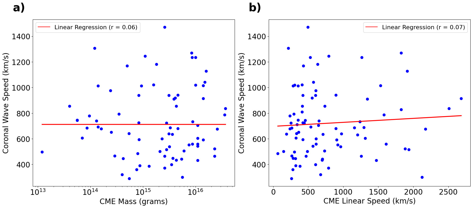
We observed that the EUV waves had differing median propagation speeds depending on classification, where those that had an accompanying CME traveled with median speed $698.75\pm 28.22$ km/s, those that did not have an accompanying CME traveled with median speed $504.15\pm 18.96$ km/s, and events where a visual inspection could not conclude the presence of a CME with median speed $572.32\pm 31.56$ km/s. From these distributions, we see that coronal waves without a CME are significantly slower and more concentrated between $300-700$ km/s, while the coronal waves with a CME are much more distributed across the axis, supported by its large standard deviation of $323.83\pm 44.71$ km/s. Then, we analyzed the correlation of the coronal wave events associated with a CME to that respective CME’s linear mass and speed (Figure 2). We find only a weak correlation between coronal wave speed and CME mass, and an even weaker (though skewed) dependence on CME speed. The linear regression lines are very weak, and the Spearman correlation coefficients are 0.02 and 0.07, respectively.

Flare X-ray properties from the GOES data provide the most important parameters of the flare energetics, meaning the statistical comparison of the X-ray and helioseismic energetics is an important step to understanding the physical processes associated with the helioseismic response. We first compare the population of isolated coronal wave flares to the population of sunquakes (Figure 3), as a potential co-excitation of coronal waves and sunquakes was the original motivation of this study. Colors in Figure 3 distinguish two populations of flare events: flares with coronal waves lacking both an accompanying CME and a sunquake (blue), and flares with an associated sunquake regardless of CME occurrence (red). The sunquake distribution is qualitatively similar to the one derived in Sharykin and Kosovichev (2020) for the sunquake events of Solar Cycle 24 — overall, flares associated with sunquakes are highly impulsive events. Their impulsive and characteristic energy release times exhibit strongly left-skewed distributions, indicating shorter time durations of their impulsive phases. Moreover, these flares range from GOES classes M to X, and generally display higher maximum values of the SXR flux time derivative, indicating powerful, energetic flares that rapidly release energy.

However, there are some slight differences from the distribution in Sharykin and Kosovichev (2020). This may be for a few reasons, most notably choices of binning, limits on the axes, and that, for purposes of this paper, we considered all 114 cataloged events as sunquakes (regardless of whether they were considered a ”sunquake candidate” due to their weak acoustic signals). The mean, median and standard deviation, with uncertainties found using the standard error propagation formula, are found in Table 2 for the impulsive phase, Table 3 for the characteristic energy release rate, Table 4 for the maximum value of the SXR flux time derivative, and Table 5 for the SXR flux/GOES class. Figure 3d revealed that isolated (not associated with a CME) coronal waves have a lower maximum SXR flux that varies between the high C and low M flare classes, spread out less than the sunquake event distribution. Moreover, we see in Figure 3a that flares with isolated coronal waves are much less impulsive, and can span from a few minutes to almost one hundred minutes. This is further supported by the characteristic energy-release time in Figure 3b, which shows a smaller, less pronounced peak that has a much wider variation than the sunquake population. This difference is more pronounced in terms of the maximum values of the SXR flux time derivative in Figure 3c, which shows that the isolated coronal wave flares have an order of magnitude lower max SXR flux time derivative than that of sunquakes.

Then we compared flares in the 2010–2022 time frame that were not associated with a sunquake or coronal wave with the population of isolated coronal wave flares previously described (Figure 4). Colors in Figure 4 highlight two populations of flare events: flares with coronal waves that did not have an accompanying CME and were not associated with a sunquake (blue), and flares that were not associated with any type of coronal wave or sunquake (green). Note that Tables 2, 3, 4 and 5 also have the mean, median, and standard deviations of these distributions as well. Figure 4a shows that isolated coronal wave events (without sunquakes) have marginally higher impulsive phase durations than events without any photospheric or coronal seismic events. However, Figure 4b indicates flares with isolated coronal waves still have a shorter characteristic growth time. Figure 4c presents a slightly higher peak in the maximum SXR flux time derivative of the isolated coronal wave events, indicative of greater energy release rates. Figure 4d shows that these events also have a consistently higher GOES flare class, meaning more intense radiation (and thus higher energy) than a flare with no sunquake or coronal wave.

Finally, we compare the same population of isolated coronal wave flares with the rest of the coronal wave population that was related to a CME (Figure 5). Colors in Figure 5 highlight two populations of flare events: flares with coronal waves that did not have an accompanying CME and were not associated with a sunquake (blue), and flares with coronal waves that did accompany a CME and were not associated with a sunquake (purple). Again, Tables 2, 3, 4 and 5 also have the mean, median, and standard deviations of these distributions.

Overall, the CME-related distributions are much wider than the sunquake flares, non-coronal wave and non-sunquake flares, and isolated coronal wave flares, as given by the comparatively high standard deviation in Figures 5a–d. For example, in Figure 5b, isolated (events without a CME) coronal-wave flare events have a standard deviation of $205.49\pm 126.35$ seconds compared to CME-related coronal wave flare events having a standard deviation of $697.70\pm 264.73$ seconds. Likewise in panel (d), isolated coronal wave flare events have a standard deviation of $2.85\times 10^{-5}\pm 1.28\times 10^{-5}$ Watts $m^{-2}s^{-1}$ while CME-related coronal wave events have a greater standard deviation of $3.12\times 10^{-3}\pm 3.12\times 10^{-3}$ Watts $m^{-2}s^{-1}$ . Figure 5a shows that isolated coronal wave flares have a shorter impulsive phase duration, meaning they are more impulsive and have faster energy release than flares that have CME-related coronal waves. Figure 5b supports this conclusion, as the distribution of the CME-related coronal wave flares is shifted and has a much smaller peak. However, the two populations have similar distributions of maximum value of the SXR flux time-derivative—which characterizes the maximal energy release rate—shown in Figure 5c. Nevertheless, the isolated coronal wave flares’ median is slightly lower than the CME-related coronal wave flares with a more pronounced peak in the distribution. Figure 5d presents CME-related coronal wave flares’ GOES class as ranging from high C to X, with a median slightly higher than that of isolated coronal wave flares and most concentrated in the middle M class. Altogether, this reveals that while isolated coronal wave flares may have faster energy release, they release overall less energy than flares that are associated with a CME.

Figure 6 presents distributions of the maximum volume emission measure and maximum temperature for each flare to illustrate further differences in magnetic energy release between the populations of CME-related and isolated coronal wave flares. The emission measure provides information about the density and volume of the hot plasma, and larger values (between $10^{46}$ and $10^{50}$ cm^-3) are characteristic of stronger flares with more substantial heating. When coupled with higher peak temperatures, these enhanced emission measures indicate a greater release of magnetic energy (Feldman et al., 1996). The temperature and emission measure of the flare events are computed using the GOES SXR flux as described in Section 2.3.2. Colors in Figure 6 highlight three populations of flare events (where sunquakes may be found in any of the three populations): flares with coronal waves that did not have an accompanying CME (red), flares with coronal waves that did accompany a CME (blue), and flare events without any coronal wave event (green). Moreover, the mean, median, and standard deviations of these distributions for the maximum emission measure histograms can also be found in Table 6 using photospheric abundances and Table 7 using coronal abundances. The same statistics are available for the flare temperatures in Table 8 using photospheric abundance and Table 9 using coronal abundance.

Figures 6a1 and 6a2 show the maximum flare emission measure and temperature using the photospheric element abundance, while 6b1 and 6b2 use the coronal element abundance. The main difference between the two temperature estimates appears only to be a scaling factor, likely from FIP-related (first ionization potential effect) differences in the abundances; elements with FIPs of less than 10 eV have abundances three to four times greater in the corona than in the photosphere (Doschek et al., 2018). However, this difference is more pronounced in the emission measure, where cooler flares ( $\sim 15$ MK) have comparable values for the max flare temperature in both photospheric and coronal abundances; however, for hotter flares ( $\sim 35$ MK), coronal abundance leads to nearly $25$ % lower derived temperatures (White et al., 2005).

Figures 6a2 and 6b2 show that CME-related coronal wave flares are the hottest, followed by isolated (without a CME) coronal wave flares and then by the other non-coronal wave flares. The non-coronal wave flare population’s temperature distribution peaks (calculated for the photosphere element abundance) around 10 MK and has the most narrow distribution of the three populations. The widest temperature distribution is the CME-related flare population, which does not have a pronounced peak in calculations for either the photosphere element abundance or the coronal element abundance and is shifted to the right, signifying higher temperatures. The isolated coronal wave flare distribution has a clear peak calculated for the coronal element abundance that is higher than that of the non-coronal wave events, but is shifted to the left of the CME-related events. The uncertainties on the medians in Tables 8 and 9 highlight that the CME-related coronal wave flare population has higher temperatures and is well-separated from the isolated coronal wave and non-coronal wave distributions. In other words, CME-related coronal wave flares have a more significant release of magnetic energy than isolated coronal wave flares because a higher temperature means more energy was released and converted into heat.

Panels (a1) and (b1) present a significant difference in the emission measure of coronal wave flares with and without a CME. Isolated coronal wave flares have the lowest emission measure and seem to fall in the same range as a general flare without any coronal wave event, while coronal wave events with a CME have significantly greater emission measure. It appears that this characteristic reveals a stark difference between the isolated coronal wave flares (median EM $6.69\times 10^{48}\pm 0.823\times 10^{48}$ cm^-3) and CME-related coronal wave flares (median EM $69.2\times 10^{48}\pm 15.9\times 10^{48}$ cm^-3); these numerical values are summarized in Table 7. The broader distribution of CME-related coronal wave flares indicates a greater amount of hot, dense plasma, a key indicator of a more substantial and energetic flare event involving a significant amount of heated material that emits intense SXR radiation. This is supported by the nature of CMEs, which are ejections of large, dense volumes of hot plasma into the heliosphere.

Moreover, we wanted to confirm the flare energy distribution for the three flare populations directly, analyzing whether the results agreed with findings from the distributions of the flare volume emission measure, temperature, and impulsivity (Figure 7). We find that the energy released by isolated coronal wave flares (median $0.0247\times 10^{30}\pm$ $0.00884\times 10^{30}$ erg) is slightly greater than that of the non-coronal wave flares (median $0.0189\times 10^{30}\pm 0.00273\times 10^{30}$ erg), but both are one to two orders of magnitude lower than the energy released by CME-related coronal wave flares (median $1.41\times 10^{30}\pm 0.381\times 10^{30}$ erg); these numerical values are summarized in Table 10. Similar to the trends in Figure 6, the energy distribution of CME-related coronal wave flares is notably broader and spans a wide range of energies, while the isolated and non-coronal wave distributions exhibit more constrained, well-defined maxima.

We also investigated the correlation of the coronal wave speeds with both maximum flare emission measure and maximum flare temperature (using both coronal and photospheric abundances) to determine whether either of these factors influences the coronal wave speeds. Figures 8a1 and 8b1 show (with some outliers) that isolated coronal wave flares that occurred between 2010 and 2013 are generally slower and have a smaller emission measure than CME-related coronal wave flares. These CME-related coronal wave flares also have a weak linear correlation between wave speed and emission measure. Figures 8a2 and 8b2 demonstrate that the slower isolated coronal wave flares are also cooler and have an even weaker linear correlation between wave speed and temperature, as the temperature and speeds of CME-related coronal wave flares are much more sparsely populated. The dark, bright, or unclear fronts for each of these coronal wave events were observed by eye for each event recorded in Nitta et al. (2013) in 171Å. The small sample of isolated coronal wave flares mostly have unclear or dark fronts, which seems to agree with both Figure 6 and Figures 8a2 and 8b2 in that these isolated wave events may be slower and cooler, thus having less energy. The emission measure versus wave speed seems to be slightly more correlated with wave speed than the temperature, with Figures 8a1 and 8b1 having Spearman correlation coefficients of 0.43 and 0.42 respectively, while 8a2 and 8b2 have correlation coefficients of 0.26 and 0.27 respectively.

4 Discussion and Conclusion

We have performed a comprehensive study on solar flares from 2010-2022 that are correlated with coronal waves (or large-scale coronal propagating fronts) to understand how they may be affected by the presence of a coronal mass ejection. We analyze GOES SXR emission and its temporal evolution for coronal-wave-associated flares, comparing with events that have an accompanying CME as well as those without. The analysis further distinguishes non-sunquake isolated coronal wave flares from flares associated with sunquakes, and from flares exhibiting neither a sunquake nor a coronal wave. By cross-referencing catalogs of sunquakes, CMEs, and coronal waves, we statistically compare these flare populations. The main results can be summarized as follows:

1.

We find that coronal waves without an observed coronal mass ejection moved more slowly than coronal waves with a coronal mass ejection. Our fitting analysis has shown that coronal waves without CMEs are concentrated at lower propagation speeds with a clear maximum in the observed distribution, whereas coronal waves with CMEs span a much broader speed distribution that is skewed towards higher propagation speeds. The distribution of flare energies confirms flares that have CMEs are more energetic than those without; this suggests a correlation where higher energy release is associated with increased wave propagation speeds. Note that these wave speeds are originally from Nitta et al. (2013) and include only dates from 2010 to 2013.
2.

Our analysis also revealed that isolated flares with coronal waves release their magnetic energy faster (i.e. more impulsive) than CME-related coronal wave flares; however, CME-related coronal wave flares have more energy. This trend was initially indicated by higher maximum values of the soft X-ray time derivative and X-ray class, but confirmed through temporal integration of the GOES SXR light curves for each recorded flare event.
3.

Our finding that CME-related flares release more energy is further supported by their significantly higher maximum flare emission measure and slightly hotter maximum flare temperature compared to isolated coronal wave flares. This may influence the apparent, but weak, correlation between coronal wave speed and emission measure or temperature.

In our initial investigation, we examined whether seismically active flares (those that produce sunquakes) can also generate coronal shockwaves from flare-accelerated particles. We also looked for similarities in the distributions of sunquake and isolated coronal wave flare events with the temporal characteristics of the flare soft X-ray emission. Although the results are not conclusive in answering the exact mechanism that generates either the flare’s helioseismic response or coronal shock waves without a CME burst, it does support the conclusion that coronal waves without an accompanying CME are driven by a process distinct from the CME model scenarios, such as those described in Downs et al. (2011, 2012, 2021) and Cohen et al. (2009).

The catalog from Nitta et al. (2013) contained only large-scale coronal propagating front speeds from 2010-2013, so further studies using speeds beyond 2013 with the time-distance method would allow us to draw better conclusions. Additionally, as mentioned by Sharykin and Kosovichev (2020), a further detailed multi-spectral study considering characteristics of the magnetic field structure and flare emission in other ranges of the electromagnetic spectrum would be promising, particularly in radio imaging. Type III radio bursts are associated with fast electron beams escaping the corona by traveling upward along magnetic field lines at near-relativistic speeds, exciting plasma emission that generates radio waves (Reid and Ratcliffe, 2014). The Expanded Owens Valley Solar Array (Gary et al., 2018) observes in the microwave regime (1-18 GHz) with temporal resolution of about 1 s at more than 100 frequency channels; moreover, they also provide solar spectral-imaging observations in high resolution, meaning it is quite easy to find the source region and the relationship between the burst and the magnetic field in that region (Tan et al., 2023). This can shed more light on what characteristics of flares, both in the pre-flare atmosphere and the flare dynamics, affect how energy is redistributed throughout the solar atmosphere.

Overall, we find evidence that the generation of coronal waves without a CME is physically distinct from those generated with a CME. The substantially lower volume emission measure is a strong indicator distinguishing coronal wave events with or without associated CMEs. Isolated coronal wave events, or flares without a CME that are associated with a coronal wave event, are more impulsive (although weaker) than populations without coronal waves or CME-related coronal waves. While the distributions of isolated coronal wave flare properties differ from those of helioseismic events, the two populations share the important characteristic of rapid energy release. Finding further evidence of flare-accelerated particles’ effect on the corona will allow for a unification of coronal seismology in the outer atmosphere with helioseismology and the propagation of acoustic waves into the Sun’s interior. Moreover, it enables a more comprehensive characterization of solar flares and eventually more accurate prediction of space weather.

The following tables show the calculated median, mean and standard deviation (with uncertainties found by error propagation) for the log-normal curve fits of the plots in each figure. Note that the tables are separated by the certain characteristic of the flare/coronal wave they highlight (i.e., coronal wave speeds, impulsive phase duration, emission measure). Moreover, coronal and photospheric abundances are divided into separate tables.

Table 1: Statistics of coronal wave speeds, in km s^-1, for different CME associations.

Category	Median	Mean	Std. Dev.
Coronal wave without CME	$504.15\pm 18.96$	$536.16\pm 23.81$	$194.08\pm 27.60$
Coronal wave with CME	$698.75\pm 28.22$	$759.60\pm 37.17$	$323.83\pm 44.71$
Possible/weak CME	$572.32\pm 31.56$	$617.87\pm 40.25$	$251.37\pm 47.39$

Table 2: Statistics of the impulsive phase duration in minutes for different flare populations.

Category	Median	Mean	Std. Dev.
Isolated coronal wave	$19.07\pm 5.05$	$29.72\pm 11.22$	$35.52\pm 20.54$
Sunquake	$4.79\pm 0.33$	$5.72\pm 0.53$	$3.72\pm 0.67$
No sunquake or coronal wave	$8.33\pm 0.86$	$9.71\pm 1.30$	$5.82\pm 1.57$
CME-related coronal wave	$29.29\pm 4.57$	$46.24\pm 10.15$	$56.51\pm 18.65$

Table 3: Statistics of the characteristic energy release time,

[df_{1-8}/dt/f]^{-1}

in seconds for different flare populations.

Category	Median	Mean	Std. Dev.
Isolated coronal wave	$147.21\pm 40.81$	$207.28\pm 79.74$	$205.49\pm 126.35$
Sunquake	$42.47\pm 3.97$	$47.71\pm 5.66$	$24.43\pm 6.44$
No sunquake or coronal wave	$229.37\pm 12.81$	$314.11\pm 24.15$	$293.88\pm 36.77$
CME-related coronal wave	$351.09\pm 63.09$	$560.56\pm 141.99$	$697.70\pm 264.73$

Table 4: Statistics of the maximum time derivative of the GOES SXR flux,

(df_{1-8}/dt)_{\mathrm{max}}

10^{-6}Wm^{-2}{s}^{-2}

for different flare populations.

Category	Median	Mean	Std. Dev.
Isolated coronal wave	$0.209\pm 0.124$	$0.436\pm 0.383$	$0.798\pm 1.000$
Sunquake	$1.450\pm 0.138$	$2.000\pm 0.261$	$1.890\pm 0.401$
No sunquake or coronal wave	$0.0571\pm 0.00537$	$0.0842\pm 0.0110$	$0.0914\pm 0.0186$
CME-related coronal wave	$0.717\pm 0.350$	$2.290\pm 1.650$	$6.950\pm 6.790$

Table 5: Statistics of the max GOES SXR flux,

(f_{1-8})_{\mathrm{max}}

10^{-5}Wm^{-2}{s}^{-1}

for different flare populations.

Category	Median	Mean	Std. Dev.
Isolated coronal wave	$1.64\pm 0.341$	$2.49\pm 0.729$	$2.85\pm 1.28$
Sunquake	$14\pm 5.87$	$22.8\pm 13.9$	$29\pm 27$
No sunquake or coronal wave	$0.595\pm 0.0491$	$0.726\pm 0.0801$	$0.509\pm 0.104$
CME-related coronal wave	$24.2\pm 12.1$	$88.4\pm 65.3$	$312\pm 312$

Table 6: Statistics of the max volume emission measure (photospheric abundance) in

10^{48}cm^{-3}

for different flare populations.

Category	Median	Mean	Std. Dev.
Isolated coronal wave	$20.5\pm 2.36$	$25.5\pm 3.91$	$18.7\pm 5.16$
CME-related coronal wave	$117\pm 17.2$	$211\pm 44.1$	$315\pm 95.2$
Non-coronal wave	$25.9\pm 1.44$	$32.1\pm 2.40$	$23.7\pm 3.18$

Table 7: Statistics of the max volume emission measure (coronal abundance) in

10^{48}cm^{-3}

for different flare populations.

Category	Median	Mean	Std. Dev.
Isolated coronal wave	$6.69\pm 0.823$	$8.38\pm 1.40$	$6.35\pm 1.89$
CME-related coronal wave	$69.2\pm 15.9$	$162\pm 54.1$	$342\pm 159$
Non-coronal wave	$7.23\pm 0.44$	$9.09\pm 0.747$	$6.93\pm 1.01$

Table 8: Statistics of the max flare temperature (photospheric abundance) in megakelvin (

MK

) for different flare populations.

Category	Median	Mean	Std. Dev.
Isolated coronal wave	$11.73\pm 0.41$	$12.32\pm 0.51$	$3.94\pm 0.53$
CME-related coronal wave	$14.54\pm 0.30$	$15.67\pm 0.39$	$6.27\pm 0.42$
Non-coronal wave	$9.58\pm 0.08$	$9.96\pm 0.09$	$2.84\pm 0.09$

Table 9: Statistics of the max flare temperature (coronal abundance) in

MK

for different flare populations.

Category	Median	Mean	Std. Dev.
Isolated coronal wave	$12.49\pm 0.30$	$13.03\pm 0.37$	$3.87\pm 0.40$
CME-related coronal wave	$14.90\pm 0.36$	$15.70\pm 0.44$	$5.22\pm 0.46$
Non-coronal wave	$10.62\pm 0.06$	$10.96\pm 0.07$	$2.78\pm 0.09$

Table 10: Statistics of the max flare energy in

10^{30}

erg for different flare populations.

Category	Median	Mean	Std. Dev.
Isolated coronal wave	$0.0247\pm 0.00884$	$0.0365\pm 0.0183$	$0.0398\pm 0.0309$
CME-related coronal wave	$1.41\pm 0.3810$	$7.06\pm 2.80$	$34.6\pm 18.3$
Non-coronal wave	$0.0189\pm 0.00273$	$0.0329\pm 0.00675$	$0.0468\pm 0.0140$

{acks}

The observational data are courtesy of the SDO/AIA, GOES, and LASCO science teams. The CME catalog is generated and maintained at the CDAW Data Center by NASA and The Catholic University of America in cooperation with the Naval Research Laboratory. SOHO is a project of international cooperation between ESA and NASA. The LCPF catalog is compiled and maintained using SDO/AIA data by Nariaki V. Nitta at the Lockheed Martin Solar and Astrophysics Laboratory.

{authorcontribution}

R.N. Bush wrote the main manuscript text and prepared figures 1-7 as well as tables 1-9. J.T. Stefan edited the main manuscript and assisted in the data collection and troubleshooting of figures 1, 3, 4, 5, and 6. A.G. Kosovichev edited the main manuscript and provided suggestions on error analysis for figures 1, 3, 4, 5, and 6. All authors reviewed the manuscript. {fundinginformation} The work was partially supported by the NSF grant 1916509, and NASA grants 80NSSC22M0162, 80NSSC23K0097, and 80NSSC25K7675. {dataavailability} The catalog of Large-scale Coronal Propagating Fronts (LCPFs) is available online at https://aia.lmsal.com/AIA˙Waves/index.html, and the original paper reporting the 2010–2013 wave speeds is available at https://doi.org/10.1088/0004-637X/776/1/58. The catalog of sunquakes from Solar Cycle 24 is available at
https://solarflare.njit.edu/sunquakes/sunquakes.html, with the original paper available at
https://doi.org/10.3847/1538-4357/ab88d1. The SOHO LASCO CME Catalog is available at https://cdaw.gsfc.nasa.gov/CME˙list/. The GOES data archive is available at https://www.ngdc.noaa.gov/stp/satellite/goes/dataaccess.html, with data analysis performed using SunPy documentation available at https://docs.sunpy.org/en/stable/generated/gallery/time˙series/goes˙xrs˙example.html. Additionally, SunPy documentation describing the calculation of temperature and the corresponding volume emission measure from GOES/XRS data is available at https://docs.sunpy.org/projects/sunkit-instruments/en/stable/api/sunkit_instruments.goes_x
rs.calculate_temperature_em.html. {ethics} {conflict} The authors declare no competing interests.

References

J. C. Allred, A. F. Kowalski, and M. Carlsson (2015) A Unified Computational Model for Solar and Stellar Flares. \apj 809 (1), pp. 104. External Links: Document, 1507.04375 Cited by: §1.
S. I. Aoki, S. Yashiro, and K. Shibata (2004) The Log-normal Distributions of Physical Quantities of Flare associated Coronal Mass Ejections (CMEs), and Flare/CME Model of Gamma-ray Bursts. arXiv e-prints, pp. astro–ph/0401352. External Links: Document, astro-ph/0401352 Cited by: §3.
M. J. Aschwanden, A. Caspi, C. M. S. Cohen, G. Holman, J. Jing, M. Kretzschmar, E. P. Kontar, J. M. McTiernan, R. A. Mewaldt, A. O’Flannagain, I. G. Richardson, D. Ryan, H. P. Warren, and Y. Xu (2019) Global Energetics of Solar Flares and Coronal Mass Ejections. In Journal of Physics Conference Series, Journal of Physics Conference Series, Vol. 1332, pp. 012002. External Links: Document Cited by: §1.
D. A. Biesecker, D. C. Myers, B. J. Thompson, D. M. Hammer, and A. Vourlidas (2002) Solar Phenomena Associated with “EIT Waves”. \apj 569 (2), pp. 1009–1015. External Links: Document Cited by: §1.
G. E. Brueckner, R. A. Howard, M. J. Koomen, C. M. Korendyke, D. J. Michels, J. D. Moses, D. G. Socker, K. P. Dere, P. L. Lamy, A. Llebaria, M. V. Bout, R. Schwenn, G. M. Simnett, D. K. Bedford, and C. J. Eyles (1995) The Large Angle Spectroscopic Coronagraph (LASCO). \solphys 162 (1-2), pp. 357–402. External Links: Document Cited by: §2.1.
J. P. Byrne, D. M. Long, P. T. Gallagher, D. S. Bloomfield, S. A. Maloney, R. T. J. McAteer, H. Morgan, and S. R. Habbal (2013) Improved methods for determining the kinematics of coronal mass ejections and coronal waves. \aap 557, pp. A96. External Links: Document, 1307.8155 Cited by: §1.
P. F. Chen (2006) The Relation between EIT Waves and Solar Flares. \apjl 641 (2), pp. L153–L156. External Links: Document Cited by: §1.
E. W. Cliver, M. Laurenza, M. Storini, and B. J. Thompson (2005) On the Origins of Solar EIT Waves. \apj 631 (1), pp. 604–611. External Links: Document Cited by: §1.
O. Cohen, G. D. R. Attrill, W. B. Manchester, and M. J. Wills-Davey (2009) Numerical Simulation of an EUV Coronal Wave Based on the 2009 February 13 CME Event Observed by STEREO. \apj 705 (1), pp. 587–602. External Links: Document, 0909.3095 Cited by: §4.
E. L. Crow and K. Shimizu (1988) Lognormal distributions: theory and applications. Dekker, New York. Cited by: §3.
V. Domingo, B. Fleck, and A. I. Poland (1995) SOHO: The Solar and Heliospheric Observatory. \ssr 72 (1-2), pp. 81–84. External Links: Document Cited by: §1.
G. A. Doschek, H. P. Warren, L. K. Harra, J. L. Culhane, T. Watanabe, and H. Hara (2018) Photospheric and Coronal Abundances in an X8.3 Class Limb Flare. \apj 853 (2), pp. 178. External Links: Document Cited by: §3.
C. Downs, I. I. Roussev, B. van der Holst, N. Lugaz, I. V. Sokolov, and T. I. Gombosi (2011) Studying Extreme Ultraviolet Wave Transients with a Digital Laboratory: Direct Comparison of Extreme Ultraviolet Wave Observations to Global Magnetohydrodynamic Simulations. \apj 728 (1), pp. 2. External Links: Document Cited by: §4.
C. Downs, I. I. Roussev, B. van der Holst, N. Lugaz, and I. V. Sokolov (2012) Understanding SDO/AIA Observations of the 2010 June 13 EUV Wave Event: Direct Insight from a Global Thermodynamic MHD Simulation. \apj 750 (2), pp. 134. External Links: Document Cited by: §4.
C. Downs, A. Warmuth, D. M. Long, D. S. Bloomfield, R. Kwon, A. M. Veronig, A. Vourlidas, and B. Vršnak (2021) Validation of Global EUV Wave MHD Simulations and Observational Techniques. \apj 911 (2), pp. 118. External Links: Document Cited by: §4.
U. Feldman, G. A. Doschek, W. E. Behring, and K. J. H. Phillips (1996) Electron Temperature, Emission Measure, and X-Ray Flux in A2 to X2 X-Ray Class Solar Flares. \apj 460, pp. 1034. External Links: Document Cited by: §3.
S. L. Freeland and B. N. Handy (1998) Data Analysis with the SolarSoft System. \solphys 182 (2), pp. 497–500. External Links: Document Cited by: §2.1.
H. A. Garcia (1994) Temperature and Emission Measure from Goes Soft X-Ray Measurements. \solphys 154 (2), pp. 275–308. External Links: Document Cited by: §2.3.2.
D. E. Gary, B. Chen, B. R. Dennis, G. D. Fleishman, G. J. Hurford, S. Krucker, J. M. McTiernan, G. M. Nita, A. Y. Shih, S. M. White, and S. Yu (2018) Microwave and Hard X-Ray Observations of the 2017 September 10 Solar Limb Flare. \apj 863 (1), pp. 83. External Links: Document, 1807.02498 Cited by: §4.
N. Gopalswamy, G. Michałek, S. Yashiro, P. Mäkelä, S. Akiyama, H. Xie, and A. Vourlidas (2024) The SOHO LASCO CME Catalog – Version 2. arXiv e-prints, pp. arXiv:2407.04165. External Links: Document, 2407.04165 Cited by: §2.1.
S. Granovsky, A. G. Kosovichev, V. M. Sadykov, G. S. Kerr, and J. C. Allred (2025) Strong Photospheric Heating Indicated by Fe I 6173 Å Line Emission during White-light Solar Flares. \apj 988 (1), pp. 74. External Links: Document, 2410.07440 Cited by: §1.
A. G. Kosovichev and V. V. Zharkova (1998) X-ray flare sparks quake inside Sun. \nat 393 (6683), pp. 317–318. External Links: Document Cited by: §1.
E. Landi, U. Feldman, and K. P. Dere (2002) CHIANTI-An Atomic Database for Emission Lines. V. Comparison with an Isothermal Spectrum Observed with SUMER. \apjs 139 (1), pp. 281–296. External Links: Document Cited by: §2.3.2.
E. Landi, M. Landini, K. P. Dere, P. R. Young, and H. E. Mason (1999) CHIANTI - an atomic database for emission lines. III. Continuum radiation and extension of the ion database. \aaps 135, pp. 339–346. External Links: Document Cited by: §2.3.2.
J. R. Lemen, A. M. Title, D. J. Akin, P. F. Boerner, C. Chou, J. F. Drake, D. W. Duncan, C. G. Edwards, F. M. Friedlaender, G. F. Heyman, N. E. Hurlburt, N. L. Katz, G. D. Kushner, M. Levay, R. W. Lindgren, D. P. Mathur, E. L. McFeaters, S. Mitchell, R. A. Rehse, C. J. Schrijver, L. A. Springer, R. A. Stern, T. D. Tarbell, J. Wuelser, C. J. Wolfson, C. Yanari, J. A. Bookbinder, P. N. Cheimets, D. Caldwell, E. E. Deluca, R. Gates, L. Golub, S. Park, W. A. Podgorski, R. I. Bush, P. H. Scherrer, M. A. Gummin, P. Smith, G. Auker, P. Jerram, P. Pool, R. Soufli, D. L. Windt, S. Beardsley, M. Clapp, J. Lang, and N. Waltham (2012) The Atmospheric Imaging Assembly (AIA) on the Solar Dynamics Observatory (SDO). \solphys 275 (1-2), pp. 17–40. External Links: Document Cited by: §1.
C. Lindsey and D. C. Braun (2000) Basic Principles of Solar Acoustic Holography - (Invited Review). \solphys 192, pp. 261–284. External Links: Document Cited by: §2.1.
C. B. Markwardt (2009) Non-linear Least-squares Fitting in IDL with MPFIT. In Astronomical Data Analysis Software and Systems XVIII, D. A. Bohlender, D. Durand, and P. Dowler (Eds.), Astronomical Society of the Pacific Conference Series, Vol. 411, pp. 251. External Links: Document, 0902.2850 Cited by: §2.1.
G. E. Moreton and H. E. Ramsey (1960) Recent Observations of Dynamical Phenomena Associated with Solar Flares. \pasp 72 (428), pp. 357. External Links: Document Cited by: §1.
D. Moses, F. Clette, J. -P. Delaboudinière, G. E. Artzner, M. Bougnet, J. Brunaud, C. Carabetian, A. H. Gabriel, J. F. Hochedez, F. Millier, X. Y. Song, B. Au, K. P. Dere, R. A. Howard, R. Kreplin, D. J. Michels, J. M. Defise, C. Jamar, P. Rochus, J. P. Chauvineau, J. P. Marioge, R. C. Catura, J. R. Lemen, L. Shing, R. A. Stern, J. B. Gurman, W. M. Neupert, J. Newmark, B. Thompson, A. Maucherat, F. Portier-Fozzani, D. Berghmans, P. Cugnon, E. L. Van Dessel, and J. R. Gabryl (1997) EIT Observations of the Extreme Ultraviolet Sun. \solphys 175 (2), pp. 571–599. External Links: Document Cited by: §1.
N. V. Nitta, W. Liu, N. Gopalswamy, and S. Yashiro (2014) The Relation Between Large-Scale Coronal Propagating Fronts and Type II Radio Bursts. \solphys 289 (12), pp. 4589–4606. External Links: Document, 1409.4754 Cited by: §1, Figure 1.
N. V. Nitta, C. J. Schrijver, A. M. Title, and W. Liu (2013) Large-scale Coronal Propagating Fronts in Solar Eruptions as Observed by the Atmospheric Imaging Assembly on Board the Solar Dynamics Observatory—an Ensemble Study. \apj 776 (1), pp. 58. External Links: Document, 1308.3544 Cited by: §1, §2.1, §2.2, §2.3.1, Figure 2, Figure 3, Figure 8, §3, item 1, §4.
S. Patsourakos and A. Vourlidas (2009) “Extreme Ultraviolet Waves” are Waves: First Quadrature Observations of an Extreme Ultraviolet Wave from STEREO. \apjl 700 (2), pp. L182–L186. External Links: Document, 0905.2164 Cited by: §1.
H. A. S. Reid and H. Ratcliffe (2014) A review of solar type iii radio bursts. Research in Astronomy and Astrophysics 14 (7), pp. 773–804. External Links: Document Cited by: §4.
V. M. Sadykov, J. T. Stefan, A. G. Kosovichev, A. M. Stejko, A. F. Kowalski, J. C. Allred, and G. S. Kerr (2024) Can Proton Beam Heating Flare Models Explain Sunquakes?. \apj 960 (1), pp. 80. External Links: Document, 2306.13162 Cited by: §1.
P. H. Scherrer, R. S. Bogart, R. I. Bush, J. T. Hoeksema, A. G. Kosovichev, J. Schou, W. Rosenberg, L. Springer, T. D. Tarbell, A. Title, C. J. Wolfson, I. Zayer, and MDI Engineering Team (1995) The Solar Oscillations Investigation - Michelson Doppler Imager. \solphys 162 (1-2), pp. 129–188. External Links: Document Cited by: §1.
P. H. Scherrer, J. Schou, R. I. Bush, A. G. Kosovichev, R. S. Bogart, J. T. Hoeksema, Y. Liu, T. L. Duvall, J. Zhao, A. M. Title, C. J. Schrijver, T. D. Tarbell, and S. Tomczyk (2012) The Helioseismic and Magnetic Imager (HMI) Investigation for the Solar Dynamics Observatory (SDO). \solphys 275 (1-2), pp. 207–227. External Links: Document Cited by: §2.1.
I. N. Sharykin and A. G. Kosovichev (2020) Sunquakes of Solar Cycle 24. \apj 895 (1), pp. 76. External Links: Document, 1911.04197 Cited by: §2.1, §2.3.1, Figure 3, §3, §3, §4.
J. Stefan and A. Kosovichev (2025) An Acoustic Model for Sunquakes Unifying the Solar Interior and Atmosphere. arXiv e-prints, pp. arXiv:2509.06848. External Links: Document, 2509.06848 Cited by: §1, §1.
J. T. Stefan and A. G. Kosovichev (2020) Estimation of Key Sunquake Parameters through Hydrodynamic Modeling and Cross-correlation Analysis. \apj 895 (1), pp. 65. External Links: Document, 1911.06839 Cited by: §1.
B. Tan, F. Chen, Y. Zhang, C. Tan, J. Huang, and Y. Yan (2023) Drifting quasi-periodic pulsations of solar microwave bursts and their physical origin. Advances in Space Research 71 (2), pp. 684–697. External Links: Document Cited by: §4.
The SunPy Community, W. T. Barnes, M. G. Bobra, S. D. Christe, N. Freij, L. A. Hayes, J. Ireland, S. Mumford, D. Perez-Suarez, D. F. Ryan, A. Y. Shih, P. Chanda, K. Glogowski, R. Hewett, V. K. Hughitt, A. Hill, K. Hiware, A. Inglis, M. S. F. Kirk, S. Konge, J. P. Mason, S. A. Maloney, S. A. Murray, A. Panda, J. Park, T. M. D. Pereira, K. Reardon, S. Savage, B. M. Sipőcz, D. Stansby, Y. Jain, G. Taylor, T. Yadav, Rajul, and T. K. Dang (2020) The sunpy project: open source development and status of the version 1.0 core package. The Astrophysical Journal 890, pp. 68–. External Links: Document, Link Cited by: §2.3.2.
R. J. Thomas, R. Starr, and C. J. Crannell (1985) Expressions to Determine Temperatures and Emission Measures for Solar X-Ray Events from Goes Measurements. \solphys 95 (2), pp. 323–329. External Links: Document Cited by: §2.3.2, §2.3.2.
B. J. Thompson, S. P. Plunkett, J. B. Gurman, J. S. Newmark, O. C. St. Cyr, and D. J. Michels (1998) SOHO/EIT observations of an Earth-directed coronal mass ejection on May 12, 1997. \grl 25 (14), pp. 2465–2468. External Links: Document Cited by: §1.
Y. Uchida (1968) Propagation of Hydromagnetic Disturbances in the Solar Corona and Moreton’s Wave Phenomenon. \solphys 4 (1), pp. 30–44. External Links: Document Cited by: §1.
C. Verbeeck, E. Kraaikamp, D. F. Ryan, and O. Podladchikova (2019) Solar Flare Distributions: Lognormal Instead of Power Law?. \apj 884 (1), pp. 50. External Links: Document Cited by: §3.
B. Vršnak, A. Warmuth, M. Temmer, A. Veronig, J. Magdalenić, A. Hillaris, and M. Karlický (2006) Multi-wavelength study of coronal waves associated with the CME-flare event of 3 November 2003. \aap 448 (2), pp. 739–752. External Links: Document Cited by: §1.
A. Warmuth, B. Vršnak, H. Aurass, and A. Hanslmeier (2001) Evolution of Two EIT/H $\alpha$ Moreton Waves. \apjl 560 (1), pp. L105–L109. External Links: Document Cited by: §1.
A. Warmuth, B. Vršnak, J. Magdalenić, A. Hanslmeier, and W. Otruba (2004) A multiwavelength study of solar flare waves. I. Observations and basic properties. \aap 418, pp. 1101–1115. External Links: Document Cited by: §1.
S. M. White, R. J. Thomas, and R. A. Schwartz (2005) Updated Expressions for Determining Temperatures and Emission Measures from Goes Soft X-Ray Measurements. \solphys 227 (2), pp. 231–248. External Links: Document Cited by: §2.3.2, §2.3.2, Figure 6, §3.