Curvature-weighted spectra anticipate dissipation peaks in decaying three-dimensional turbulence

We consider freely decaying, incompressible turbulence governed by the 3D Navier–Stokes equations in a periodic box of size $L=2\pi$:

	$\displaystyle\partial_{t}\mathbf{u}+(\mathbf{u}\!\cdot\!\nabla)\mathbf{u}$	$\displaystyle=-\nabla p+\nu\nabla^{2}\mathbf{u},$		(4)
	$\displaystyle\nabla\cdot\mathbf{u}$	$\displaystyle=0,$		(5)

where $\mathbf{u}(\mathbf{x},t)$ is the velocity, $p(\mathbf{x},t)$ is the kinematic pressure, and $\nu$ is the kinematic viscosity. The vorticity is $\boldsymbol{\omega}=\nabla\times\mathbf{u}$. We use the volume average $\langle\cdot\rangle\equiv(2\pi)^{-3}\int_{[0,2\pi)^{3}}(\cdot)\,d\mathbf{x}$. The kinetic energy and dissipation rate are

$$K(t)\equiv\frac{1}{2}\langle|\mathbf{u}|^{2}\rangle,\qquad\varepsilon(t)\equiv-\frac{dK}{dt}=\nu\langle|\nabla\mathbf{u}|^{2}\rangle.$$

(6)

We solve Eqs. (4)–(5) using a massively parallel pseudo-spectral method with FFTW–MPI slabs and a real-to-complex layout [11]. The velocity field is represented by a Fourier series

$$\mathbf{u}(\mathbf{x},t)\;=\;\sum_{\boldsymbol{\kappa}}\hat{\mathbf{u}}(\boldsymbol{\kappa},t)\,e^{\,i\boldsymbol{\kappa}\cdot\mathbf{x}},\qquad\boldsymbol{\kappa}=(\kappa_{x},\kappa_{y},\kappa_{z})\in\mathbb{Z}^{3},$$

(7)

on an $N^{3}$ collocation grid. Spectral derivatives are computed exactly, e.g., $\partial_{j}u_{i}\leftrightarrow i\kappa_{j}\hat{u}_{i}$. The nonlinear term

$$\mathbf{N}(\mathbf{x},t)\;\equiv\;(\mathbf{u}\!\cdot\!\nabla)\mathbf{u}$$

(8)

is assembled in physical space from $u_{i}$ and the spectral derivatives, transformed to Fourier space, and then projected to enforce incompressibility. In Fourier space, the evolution for each mode can be written as

$$\partial_{t}\hat{\mathbf{u}}(\boldsymbol{\kappa},t)\;=\;-\widehat{\mathbf{N}}_{\perp}(\boldsymbol{\kappa},t)-\nu|\boldsymbol{\kappa}|^{2}\hat{\mathbf{u}}(\boldsymbol{\kappa},t),$$

(9)

where $\widehat{\mathbf{N}}_{\perp}(\boldsymbol{\kappa},t)=\mathbf{P}(\boldsymbol{\kappa})\,\widehat{\mathbf{N}}(\boldsymbol{\kappa},t)$, and $\mathbf{P}$ is the Leray projector

$$\mathbf{P}(\boldsymbol{\kappa})=\mathbf{I}-\boldsymbol{\kappa}\boldsymbol{\kappa}^{\top}/|\boldsymbol{\kappa}|^{2},\qquad(\boldsymbol{\kappa}\neq\mathbf{0}),$$

(10)

which removes pressure and enforces $\boldsymbol{\kappa}\!\cdot\!\hat{\mathbf{u}}=0$ [10, 2].

Dealiasing is performed by the standard two-thirds rule in a box sense during time marching: Fourier coefficients are set to zero whenever any component satisfies $|\kappa_{i}|>N/3$. Time integration uses a classical fourth-order Runge–Kutta scheme with an integrating factor for the viscous term [18, 6]. Velocity and vorticity snapshots are written at regular intervals for post-processing; per-rank storage enables parallel I/O and exact reconstruction consistent with the FFTW–MPI decomposition.

From saved snapshots we compute isotropic shell sums of the energy spectrum $E(k,t)$, the enstrophy spectrum $\mathcal{Z}(k,t)$, the dissipation spectrum $D(k,t)$, and the shell-summed curl-of-vorticity spectrum $\mathcal{C}_{4}(k,t)$. We denote the wavevector magnitude by $\kappa\equiv|\boldsymbol{\kappa}|$ and define integer shells by

$$k\equiv\mathrm{round}(\kappa),\qquad\mathcal{S}_{k}\equiv\{\boldsymbol{\kappa}:\mathrm{round}(|\boldsymbol{\kappa}|)=k\}.$$

(11)

With the real-to-complex plane weights denoted by $w_{\boldsymbol{\kappa}}$, the shell-summed energy spectrum is defined as

$$E(k,t)=\frac{1}{2}\sum_{\boldsymbol{\kappa}\in\mathcal{S}_{k}}w_{\boldsymbol{\kappa}}\bigl|\hat{\mathbf{u}}(\boldsymbol{\kappa},t)\bigr|^{2},\qquad\sum_{k}E(k,t)=K(t).$$

(12)

The shell-summed enstrophy spectrum is

$$\mathcal{Z}(k,t)=\frac{1}{2}\sum_{\boldsymbol{\kappa}\in\mathcal{S}_{k}}w_{\boldsymbol{\kappa}}\bigl|\hat{\boldsymbol{\omega}}(\boldsymbol{\kappa},t)\bigr|^{2}=\frac{1}{2}\sum_{\boldsymbol{\kappa}\in\mathcal{S}_{k}}w_{\boldsymbol{\kappa}}|\boldsymbol{\kappa}|^{2}\bigl|\hat{\mathbf{u}}(\boldsymbol{\kappa},t)\bigr|^{2}.$$

(13)

The dissipation spectrum is evaluated consistently from the calibrated velocity spectrum as

$$D(k,t)=2\nu k^{2}E(k,t),\qquad\varepsilon(t)=\sum_{k}D(k,t),$$

(14)

where $k$ denotes the shell-center wavenumber used in the binned spectra. Similarly, the shell-summed curl-of-vorticity spectrum is defined by

$$\mathcal{C}_{4}(k,t)=\frac{1}{2}\sum_{\boldsymbol{\kappa}\in\mathcal{S}_{k}}w_{\boldsymbol{\kappa}}\left|\widehat{\nabla\times\boldsymbol{\omega}}(\boldsymbol{\kappa},t)\right|^{2}=\frac{1}{2}\sum_{\boldsymbol{\kappa}\in\mathcal{S}_{k}}w_{\boldsymbol{\kappa}}|\boldsymbol{\kappa}|^{4}\bigl|\hat{\mathbf{u}}(\boldsymbol{\kappa},t)\bigr|^{2},$$

(15)

where the last equality uses incompressibility. Because shells are formed by integer binning, the frequently used relations

$$\mathcal{Z}(k,t)\simeq k^{2}E(k,t),\qquad\mathcal{C}_{4}(k,t)\simeq k^{4}E(k,t)$$

(16)

should be understood as shell-center shorthand expressions rather than exact identities for the binned spectra. This distinction is important for high-wavenumber-weighted diagnostics, where shell-center and modal-weighted definitions can differ slightly inside a finite-width shell.

To quantify interscale transfer we compute the transfer function directly from modal transfers in Fourier space:

$$T(k,t)=-\sum_{\boldsymbol{\kappa}\in\mathcal{S}_{k}}{\mathfrak{R}}\!\left\{\hat{\mathbf{u}}^{\ast}(\boldsymbol{\kappa},t)\cdot\widehat{\mathbf{N}}_{\perp}(\boldsymbol{\kappa},t)\right\},$$

(17)

where $\mathbf{N}=(\mathbf{u}\!\cdot\!\nabla)\mathbf{u}$ and $\widehat{\mathbf{N}}_{\perp}$ is defined in (9)–(10). To avoid notational conflict with the kinetic energy $K(t)$, the cumulative flux is written with cutoff variable $q$:

$$\Pi(q,t)\;=\;-\sum_{m\leq q}T(m,t),$$

(18)

so that $\Pi(q_{\max},t)\approx 0$ and $\sum_{k}T(k,t)\approx 0$ provide discrete conservation diagnostics (up to round-off).

For the post-processing of isotropic spectra and transfer/flux, we apply a spherical two-thirds analysis mask and record it as a binary column mask in the spectra output; unless stated otherwise, all shell sums, peak searches, and plots are restricted to shells with mask$=1$. The mask keeps only modes with $\kappa\leq K_{\mathrm{cut}}\equiv\lceil(2/3)K_{\max}\rceil$ (with $K_{\max}=N/2$) and therefore differs from the box two-thirds cutoff enforced during time marching. Because FFTW stores only half of the spectrum in the real-to-complex layout, contributions are weighted so that the $k_{z}=0$ and Nyquist planes carry a unit weight while the remaining planes carry weight $2$, ensuring exact counting of conjugate pairs. With our FFT normalization, $\sum_{k}E(k,t)$ is equal to the volume-averaged kinetic energy $K(t)$. We accumulate shell sums using Kahan summation to reduce floating-point cancellation [14].

We compare five freely decaying incompressible flows, each initialized in the periodic box $[0,2\pi]^{3}$. The cases are designed to span markedly different symmetries and large-scale organizations: a canonical nonhelical benchmark (TGV), helical structured flows (ABC-based), an ABC flow with an additional random-phase low-$k$ component, and a classical high-symmetry configuration known to generate intense small-scale activity (Kida–Pelz). Unless otherwise noted, all initial fields have zero spatial mean, and the subsequent evolution is purely decaying (no forcing).

The Taylor–Green vortex is a canonical nonhelical flow with strong symmetries and is widely used as a transition-to-turbulence benchmark; its early evolution is characterized by the formation and roll-up of vortex sheets, followed by rapid generation of smaller scales. The Arnold–Beltrami–Childress (ABC) flow is a canonical helical large-scale flow. In its standard form it is a Beltrami flow, with vorticity aligned with velocity mode by mode, and it provides a convenient way to study how helical large-scale organization influences subsequent small-scale development. The Kida–Pelz configuration is a high-symmetry flow known for rapid gradient amplification and intense small-scale generation.

The baseline set of simulations (cases (a)–(f)) is performed in the periodic domain $[0,2\pi]^{3}$ at viscosity $\nu=10^{-3}$. To probe viscosity dependence in a controlled setting, we additionally repeat the Taylor–Green vortex (TGV) initial condition at a lower viscosity $\nu=2.5\times 10^{-4}$ and at a higher viscosity $\nu=10^{-2}$ (see Sec. V.6). The base resolution is $N^{3}=512^{3}$ for cases (a)–(e) and for the high-viscosity TGV run, while companion $N^{3}=1024^{3}$ runs are performed for Kida–Pelz (case (f)) and for the low-viscosity TGV run in order to avoid cutoff-proximate peak locking in curvature-weighted spectra. Time integration uses a fixed time step $\Delta t=10^{-3}$. Velocity (and, when needed, vorticity) snapshots are saved every $n_{\rm out}=50$ time steps for post-processing, corresponding to an output interval $\Delta t_{\rm out}=5\times 10^{-2}$. The same spectral post-processing pipeline is applied to all cases (Sec. II), including the isotropic shell averaging conventions, the spherical two-thirds analysis mask, and transfer/flux diagnostics.

Because our focus is on timing relations and relative lead/lag measures, we choose the final integration time $t_{\rm end}$ in each case so that the dissipation episode is fully captured and the subsequent decay is sufficiently sampled. Specifically, we integrate up to $t_{\rm end}=60$ for the multi-ABC cases (a,b), $t_{\rm end}=120$ for the ABC+random low-$k$ case (c), and $t_{\rm end}=20$ for the baseline TGV and Kida–Pelz runs (d–f). For the viscosity-variation TGV runs, we integrate up to $t_{\rm end}=16$ for $\nu=2.5\times 10^{-4}$ and up to $t_{\rm end}=12$ for $\nu=10^{-2}$.

For cross-case comparisons of amplitude-based quantities derived from spectra (e.g., $\varepsilon(t)$ and scale measures), we adopt the same calibration convention as in Ref. [21]: the spectra are rescaled such that the total kinetic energy at the first post-processed snapshot equals a reference value $K_{0}=1/8$. This calibration does not affect peak wavenumbers such as $k_{\rm peak}[\,|\nabla\times\boldsymbol{\omega}|^{2}\,]$, and therefore does not alter the temporal ordering statements central to this work.

From the stored velocity snapshots, we construct isotropic (shell-summed) spectra in the periodic cube $[0,2\pi]^{3}$. As in our PRF Letter [21], shells are formed by binning Fourier modes by the integer $k=\mathrm{round}(|\boldsymbol{\kappa}|)$ and accumulating plane-weighted sums appropriate for real-to-complex FFT layouts. For the analysis, we additionally apply a spherical two-thirds mask and record it as a binary column mask in the spectra output (we restrict sums and peak searches to shells with mask$=1$ unless stated otherwise). We denote the maximum retained shell by

$$k_{\max}^{(\mathrm{mask})}\equiv\max\{k:\texttt{mask}(k)=1\},$$

(25)

which corresponds to the familiar spherical two-thirds cutoff (for $N=512$, $k_{\max}^{(\mathrm{mask})}=171$).

To enable a consistent comparison across different initial conditions, we use a constant calibration factor $\alpha$ that rescales the spectra so that the total kinetic energy at the earliest stored time matches a target value $K_{0}$:

$$\alpha\;=\;\frac{K_{0}}{\sum_{k}E(k,t_{0})},\qquad E(k,t)\;\leftarrow\;\alpha\,E(k,t).$$

(26)

In the present study we take $K_{0}=1/8$, which coincides with the standard unit-amplitude TGV energy in $[0,2\pi]^{3}$. All derived quantities below (including $\varepsilon$, $\eta$, and $R_{\lambda}$) are computed consistently from the calibrated spectra.

We track the standard spectral diagnostics of decaying turbulence: the kinetic energy spectrum $E(k,t)$, the dissipation density

$$D(k,t)\;=\;2\nu k^{2}E(k,t),$$

(27)

and the dissipation rate

$$\varepsilon(t)\;=\;\sum_{k}D(k,t)\;=\;2\nu\sum_{k}k^{2}E(k,t).$$

(28)

We also analyze the nonlinear transfer spectrum $T(k,t)$ and the cumulative flux

$$\Pi(q,t)\;=\;-\sum_{m\leq q}T(m,t),$$

(29)

so that $|\Pi(q,t)|$ measures the magnitude of interscale transfer across the cutoff wavenumber $q$.

The central object of this work is the shell-summed curl-of-vorticity spectrum $\mathcal{C}_{4}(k,t)$, defined in Eq. (15) with $\boldsymbol{\omega}\equiv\nabla\times\mathbf{u}$. For incompressible flow, $\nabla\cdot\mathbf{u}=0$ implies $\nabla\times\boldsymbol{\omega}=-\nabla^{2}\mathbf{u}$, so $\mathcal{C}_{4}(k,t)$ corresponds to the modal $|\boldsymbol{\kappa}|^{4}|\hat{\mathbf{u}}|^{2}$ weight and is denoted by the shorthand

$$\mathcal{C}_{4}(k,t)\simeq k^{4}E(k,t)$$

(30)

when expressed in terms of the integer shell center. This $k^{4}$ weighting accentuates the incipient formation of high-curvature structures (tightly wound tubes and rolled-up sheets), which, as we show below, advances and saturates in wavenumber before $\varepsilon(t)$ reaches its maximum.

We monitor four complementary measures of the evolving length scales. First, the instantaneous Kolmogorov scale is

$$\eta(t)\;=\;\big(\nu^{3}/\varepsilon(t)\big)^{1/4}.$$

(31)

Second, the integral scale is evaluated from the isotropic spectrum as

$$L_{\mathrm{int}}(t)\;=\;\frac{\pi}{2\sum_{k}E(k,t)}\sum_{k\geq 1}\frac{E(k,t)}{k},$$

(32)

which emphasizes the energy-containing range. Third, the Taylor microscale is computed as

$$\lambda(t)\;=\;\left(\frac{\sum_{k}E(k,t)}{\sum_{k}k^{2}E(k,t)}\right)^{1/2},$$

(33)

and with $u^{\prime}(t)=\sqrt{\tfrac{2}{3}\sum_{k}E(k,t)}$ we define the Taylor-scale Reynolds number

$$R_{\lambda}(t)\;=\;\frac{u^{\prime}(t)\,\lambda(t)}{\nu}.$$

(34)

To quantify the non-dimensional dissipation level in this unsteady decay, we also report

$$C_{\varepsilon}(t)\;=\;\frac{\varepsilon(t)L_{\mathrm{int}}(t)}{u^{\prime}(t)^{3}}.$$

(35)

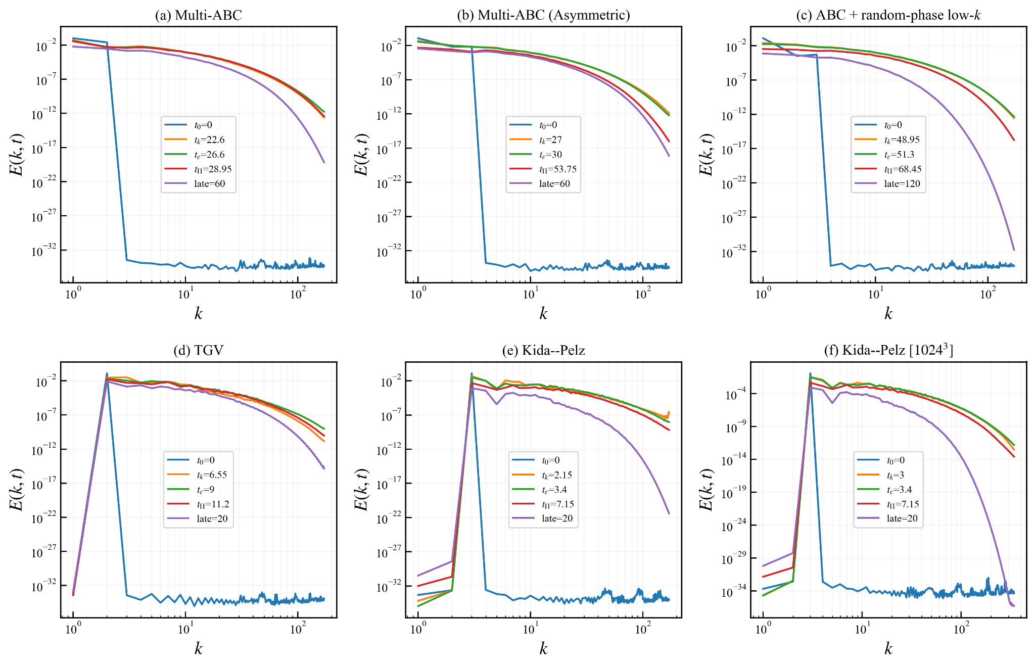
This quantity is useful in unsteady turbulence because it indicates how far the decay departs from a quasi-equilibrium picture in which a nearly constant normalized dissipation might be expected. Finally, to quantify resolution, we track the standard criterion $k_{\max}\eta(t)$, where we follow Ref. [21] and define the maximum wavenumber by the Nyquist value $k_{\max}=(N/2)\,2\pi/L$ (thus $k_{\max}=N/2$ in our $L=2\pi$ domain). In Fig. 6 we plot $R_{\lambda}(t)$ together with $k_{\max}\eta(t)$. All cases satisfy $k_{\max}\eta(t)\gtrsim\mathcal{O}(1)$ throughout the time intervals analyzed, and the minimum typically occurs near the dissipation peak. Figure 7 summarizes the concurrent evolution of $L_{\mathrm{int}}(t)$, $\lambda(t)$, $\eta(t)$, $\varepsilon(t)$, and $C_{\varepsilon}(t)$, highlighting that $\eta(t)$ reaches its minimum at $t=t_{\varepsilon}$ while the large-scale measures evolve more gradually. Representative velocity spectra at selected times are shown in Appendix Fig. A2. For each case, we plot $E(k,t)$ at $t=0$, $t_{k}$, $t_{\varepsilon}$, $t_{\Pi}$, and a late-time snapshot. These spectra show how the initially large-scale energy distribution broadens toward higher wavenumbers during the transient decay and provide a spectral complement to the scale and dissipation histories in Fig. 7.

To quantify how far toward small scales a given diagnostic has progressed, we introduce several $k$-metrics for a nonnegative shell spectrum $S(k,t)$. The most direct measure is the peak wavenumber

$$k_{\mathrm{peak}}[S](t)\;\equiv\;\arg\max_{k\geq k_{\min}}S(k,t),$$

(36)

where we take $k_{\min}=1$. We also use the centroid scale

$$k_{\mathrm{centroid}}[S](t)\;\equiv\;\frac{\sum_{k}k\,S(k,t)}{\sum_{k}S(k,t)},$$

(37)

and the weighted quantile scale $k_{q}[S](t)$ defined by the cumulative weight:

$$k_{q}[S](t)\;\equiv\;\min\left\{k:\frac{\sum_{m\leq k}S(m,t)}{\sum_{m}S(m,t)}\geq q\right\},\qquad 0<q<1.$$

(38)

In particular, we will refer frequently to $k_{95}[S](t)$.

In the present work, we apply these definitions to two spectra:

1. 1.

   $S(k,t)=\mathcal{C}_{4}(k,t)$ (the curl-of-vorticity/palinstrophy-related spectrum), and

2. 2.

   $S(k,t)=|\Pi(k,t)|$ (the magnitude of the cumulative flux).

Figures 9–14 show the time evolution of the corresponding $k$-metrics for all cases: (a) Multi-ABC, (b) Multi-ABC (Asymmetric), (c) ABC + random-phase low-$k$, (d) TGV, (e) Kida–Pelz, and (f) Kida–Pelz [1024³], together with $\varepsilon(t)$. Across initial conditions, the different definitions (peak/centroid/quantile) yield consistent qualitative trends, with the peak metric providing the most direct “advance-and-level-off” indicator.

We define the dissipation peak time as

$$t_{\varepsilon}\;\equiv\;\arg\max_{t}\,\varepsilon(t).$$

(39)

For the peak-based diagnostics, we define the characteristic times by the maximum-attainment times of the peak scales:

	$\displaystyle t_{k}$	$\displaystyle\;\equiv\;\arg\max_{t}\,k_{\mathrm{peak}}[\mathcal{C}_{4}](t),$		(40)
	$\displaystyle t_{\Pi}$	$\displaystyle\;\equiv\;\arg\max_{t}\,k_{\mathrm{peak}}[|\Pi|](t).$		(41)

When the maximum is attained over multiple consecutive outputs (a plateau), we take the earliest occurrence. For the TGV this is consistent with the “advance-and-level-off” onset time used in our Letter, because the rise of $k_{\mathrm{peak}}[\mathcal{C}_{4}](t)$ terminates in a short plateau near its maximum.

For visualization and as auxiliary reference values in the $Q$-snapshot figures (Figs. 1–5), we also report reaching times for more global metrics such as $k_{\mathrm{centroid}}$ and $k_{95}$. For a generic $k$-metric $k_{m}(t)$, we define $k_{m}^{\varepsilon}\equiv k_{m}(t_{\varepsilon})$ and, for a threshold $q\in(0,1)$,

$$t_{m,q}\;\equiv\;\min\left\{t:\;\;k_{m}(t^{\prime})\geq q\,k_{m}^{\varepsilon}\;\;\forall t^{\prime}\in[t,t+M\Delta t_{out}]\right\},$$

(42)

where $\Delta t_{out}$ is the output interval and we take $M=3$. In the snapshots we denote $t_{c}\equiv t_{\,k_{\mathrm{centroid}}[\mathcal{C}_{4}],\,q}$ and $t_{95}\equiv t_{\,k_{95}[\mathcal{C}_{4}],\,q}$ with $q=0.9$. Because the reaching-time criterion depends on the choice of $(q,M)$, we use $t_{c}$ and $t_{95}$ only as auxiliary markers and do not rely on them for the primary ordering arguments.

All characteristic times reported in this work are extracted from time series sampled at the output cadence $\Delta t_{\rm out}=5\times 10^{-2}$ (Sec. III.2). Therefore, $t_{k}$, $t_{\varepsilon}$, and $t_{\Pi}$ are quantized in steps of $\Delta t_{\rm out}$ and carry an intrinsic temporal discretization uncertainty of ${\cal O}(\Delta t_{\rm out})$. Conservatively, we take $|\delta t_{k}|,|\delta t_{\varepsilon}|,|\delta t_{\Pi}|\leq\Delta t_{\rm out}$, which implies $|\delta\Delta t_{k\varepsilon}|,|\delta\Delta t_{\varepsilon\Pi}|\leq 2\Delta t_{\rm out}$ for the lead/lag measures. In all cases summarized in Table 1, the observed separations exceed this bound; in particular, the smallest lead time $\Delta t_{k\varepsilon}=0.40$ corresponds to $8\,\Delta t_{\rm out}$, so the ordering is robust to the output cadence.

The peak-based characteristic times are extracted from the raw, unsmoothed shell spectra. We use the raw spectra because smoothing would introduce an additional parameter and could mask cutoff-proximate peak locking, which is itself an important resolution diagnostic for high-wavenumber-weighted spectra. When the maximum is attained over multiple consecutive output times, we take the earliest occurrence, consistent with the interpretation of $t_{k}$ as the end of the initial advance of the peak scale.

In all cases of Figs. 9–14, $t_{k}$ consistently precedes $t_{\varepsilon}$, while $t_{\Pi}$ occurs later than $t_{\varepsilon}$, establishing the ordering $t_{k}<t_{\varepsilon}<t_{\Pi}$ across the tested initial conditions. The centroid- and quantile-type measures ($k_{\mathrm{centroid}}$ and $k_{95}$) exhibit the same qualitative behavior, providing an additional robustness check beyond a single peak definition.

Because $\mathcal{C}_{4}(k,t)$ involves a strong $k^{4}$ weighting, peak-based indicators can be particularly sensitive to finite-resolution effects in the high-$k$ range. In extreme transient states, this sensitivity may lead to spurious peak detection if the argmax is influenced by spectral content close to the analysis cutoff. To assess this possibility, we explicitly inspect $\mathcal{C}_{4}(k,t)$ at representative times and mark the detected peak locations, as summarized in Fig. 8.

For the $512^{3}$ ABC-based cases and the TGV at the baseline viscosity $\nu=10^{-3}$, the spectrum exhibits a clear maximum of $\mathcal{C}_{4}(k,t)$ that is well separated from the cutoff. In contrast, for the Kida–Pelz case at $512^{3}$, the instantaneous argmax can approach $k_{\max}^{(\mathrm{mask})}$ during the early transient, indicating a cutoff-proximate “locking” of the peak. This behavior is visualized explicitly in Fig. 8(e) and reflects the combination of intense small-scale generation in the Kida–Pelz flow and the strong high-$k$ bias inherent in the $k^{4}$ weighting.

In this work we treat cutoff-proximate peaks as a resolution warning rather than as a feature to be “corrected” by an alternative peak definition. This inspection protocol is applied throughout the paper to all simulations reported here, including the viscosity-variation TGV runs in Sec. V.6. When cutoff-proximate locking is encountered (as in the $512^{3}$ Kida–Pelz case and the low-viscosity TGV case), we do not attempt to suppress it by an ad hoc restriction of the peak-search interval; instead, we treat it as a resolution warning and rely on a higher-resolution companion simulation for quantitative comparison.

Accordingly, to verify that the near-cutoff peak locking observed in the $512^{3}$ Kida–Pelz run is not physical, we performed a companion simulation at $1024^{3}$. As shown in Fig. 8(f), the higher-resolution spectrum exhibits a well-defined peak away from the cutoff and shows no tendency toward high-$k$ locking. This confirms that the issue observed at $512^{3}$ originates from limited resolution rather than from the underlying dynamics.

Based on this assessment, the Kida–Pelz results discussed in the remainder of this paper are taken from the $1024^{3}$ simulation, while the $512^{3}$ case is retained solely to demonstrate the resolution sensitivity of peak detection in curvature-weighted spectra.

We begin by confirming that all runs are adequately resolved over the time intervals analyzed. Figure 6 shows the time series of the Taylor-scale Reynolds number $R_{\lambda}(t)$ together with the resolution indicator $k_{\max}\eta(t)$, where $k_{\max}=(N/2)\,2\pi/L$ is the Nyquist wavenumber (as in Ref. [21]) and $\eta(t)=(\nu^{3}/\varepsilon(t))^{1/4}$ is the Kolmogorov length. For all $512^{3}$ cases (Multi-ABC, Multi-ABC asymmetric, ABC+random-phase low-$k$, TGV, and Kida–Pelz), $k_{\max}\eta(t)$ remains above unity throughout the evolution, including around the dissipation episode, indicating that the smallest dynamically relevant scales are captured. The concomitant decrease of $R_{\lambda}(t)$ during the dissipation surge reflects the rapid development of small scales and the accompanying increase of the characteristic gradients. The increase of $R_{\lambda}$ at early times in some cases should not be interpreted as evidence of continuing external production. After initialization, all runs evolve without forcing and satisfy a freely decaying energy budget. The early-time rise of $R_{\lambda}$ instead reflects a transient cascade-development stage in which $u^{\prime}$, $\lambda$, and the small-scale gradients evolve at different rates while the flow reorganizes toward its strongest dissipative state.

For the Kida–Pelz initial condition, we additionally performed a $1024^{3}$ simulation (shown as the high-resolution counterpart in Fig. 6) to address a peak-detection issue in the curvature-weighted spectrum (discussed below). As expected, the higher-resolution run provides a substantially larger $k_{\max}\eta(t)$ margin over the entire time interval, which helps disentangle physical peak motion from finite-resolution artifacts.

Figure 7 summarizes the evolution of representative scale measures $L_{\mathrm{int}}(t)$, the Taylor microscale $\lambda(t)$, the Kolmogorov scale $\eta(t)$, the dissipation rate $\varepsilon(t)$, and the normalized dissipation coefficient $C_{\varepsilon}(t)$ for all cases. The additional $C_{\varepsilon}(t)$ row is included because the present flows are unsteady and can depart from classical quasi-equilibrium dissipation phenomenology. The plotted $C_{\varepsilon}(t)$ histories are not approximately flat: in most cases $C_{\varepsilon}(t)$ changes markedly through the approach to $t_{\varepsilon}$ and continues to evolve during the subsequent decay. This non-constant behavior supports the non-equilibrium interpretation of the present decays and motivates treating dissipation-peak timing as a transient diagnostic rather than as a quasi-steady estimate. Across initial conditions, the same qualitative pattern is observed: as the flow transitions from its initially organized large-scale state toward a turbulent, volume-filling state, the energy-containing scale $L_{\mathrm{int}}$ and the intermediate scale $\lambda$ decrease, while $\eta$ decreases toward its minimum near the dissipation peak and then increases during late-time decay.

The principal difference across cases is the characteristic time window over which this transient unfolds. The structured ABC-based initial conditions (Multi-ABC and its asymmetric variant) exhibit a comparatively rapid onset of small-scale activity followed by a long decay, whereas the ABC+random-phase low-$k$ case develops and dissipates more slowly, consistent with the prolonged persistence of large-scale organization seen in the $Q$-criterion snapshots (Sec. III). The TGV evolution reproduces the canonical timescale separation reported previously [21], while the Kida–Pelz flow produces strong gradients very rapidly, in line with the known propensity of this highly symmetric configuration to generate intense small-scale structures [1, 3].

These scale trends provide an important backdrop for interpreting curvature-weighted spectral indicators: the precursor times identified below consistently occur during the phase in which $\eta(t)$ is still decreasing and the flow morphology is transitioning toward filament/tube-dominated structures.

Appendix Fig. A2 complements Fig. 7 by showing representative velocity energy spectra $E(k,t)$ at $t=0$, $t_{k}$, $t_{\varepsilon}$, $t_{\Pi}$, and a late-time snapshot for each case. These spectra show directly how kinetic energy broadens from the initial large-scale distribution toward higher wavenumbers during the transient decay.

A central observable in this work is the curvature-weighted spectrum $\mathcal{C}_{4}(k,t)$ (equivalently $k^{4}E(k)$ for incompressible flow), and the associated peak/centroid/quantile wavenumber measures introduced in Sec. IV. Because $\mathcal{C}_{4}(k,t)$ strongly emphasizes high wavenumbers, its instantaneous argmax can be particularly sensitive to finite-resolution effects near the analysis cutoff $k_{\max}^{(\mathrm{mask})}$. Following the inspection protocol described in Sec. IV.6, we therefore perform an explicit spike inspection: we examine representative spectra and verify whether the detected maximizer lies well inside the resolved range. If the maximizer lies at (or very close to) $k_{\max}^{(\mathrm{mask})}$, we interpret this as a resolution warning and rely on a higher-resolution companion simulation for quantitative extraction of characteristic times. Importantly, we do not remove, trim, or otherwise exclude peaks; the inspection is used only to flag cutoff-proximate peak locking.

Figure 8 presents representative inspections of $\mathcal{C}_{4}(k,t)$ at selected times, with the detected peak marked. For the Multi-ABC, Multi-ABC (Asymmetric), ABC+random-phase low-$k$, and TGV cases, the spectrum exhibits a well-defined maximum at intermediate-to-small scales at the inspected time, and the peak is clearly separated from $k_{\max}^{(\mathrm{mask})}$ (the spherical two-thirds cutoff). In contrast, for the Kida–Pelz case at $512^{3}$, the maximizer can approach $k_{\max}^{(\mathrm{mask})}$ during the early transient, indicating cutoff-proximate peak locking [Fig. 8(e)]. This endpoint hit is also visible in the time-series view in Fig. 13, where $k_{\mathrm{peak}}[\mathcal{C}_{4}](t)$ can reach $k_{\max}^{(\mathrm{mask})}$. Accordingly, we use the $1024^{3}$ Kida–Pelz data (Figs. 8(f) and 14) as the reference for the Kida–Pelz precursor analysis, while retaining the $512^{3}$ case only to illustrate this finite-resolution failure mode.

We now present the main comparative results. Figures 9–14 show the time evolution of the characteristic wavenumber measures derived from the curvature-weighted spectrum $\mathcal{C}_{4}(k,t)$ together with the dissipation rate $\varepsilon(t)$ (and, in the corresponding flux panels, the characteristic measures derived from $|\Pi(q,t)|$). The vertical markers indicate the characteristic times defined in Sec. IV: $t_{k}$ for the curvature-weighted precursor, $t_{\varepsilon}$ for the dissipation peak, and $t_{\Pi}$ for the largest-flux-peak scale time.

Across all cases, the precursor time associated with the curvature-weighted spectrum occurs first:

$$t_{k}<t_{\varepsilon},$$

(43)

and the flux-related time occurs last,

$$t_{\varepsilon}<t_{\Pi},$$

(44)

thereby establishing the robust ordering

$$t_{k}<t_{\varepsilon}<t_{\Pi}$$

(45)

beyond the TGV setting of Ref. [21]. Importantly, this conclusion does not rely on a single, potentially noisy definition of a “peak”. Figures 9–14 show that alternative wavenumber characterizations—including centroid-type and quantile-type measures (e.g., $k_{c}$ and $k_{95}$, and their associated characteristic times)—exhibit the same qualitative advance relative to $t_{\varepsilon}$, providing evidence that the precursor is a robust feature of the overall spectral redistribution rather than a fragile local maximizer.

The comparative view also clarifies how initial-condition-dependent transients modulate the magnitude of the lead time while preserving the ordering. In the ABC+random-phase low-$k$ case, the entire evolution is stretched, and both $t_{k}$ and $t_{\varepsilon}$ occur later than in the structured ABC-based cases; nevertheless, the curvature-weighted measures still rise and stabilize before the dissipation maximum. In the Kida–Pelz configuration, the precursor develops extremely early, consistent with the rapid formation of tightly curved tubes and sheets seen in the $Q$-criterion visualizations (Sec. III), and the high-resolution run confirms that this early stabilization is a physical feature rather than an artifact of insufficient small-scale resolution.

Finally, the flux-based characteristic measures evolve more slowly than their curvature-weighted counterparts, reflecting the fact that $|\Pi|$ is an integral indicator of net interscale transfer and therefore lags the initial formation of high-curvature structures that viscosity will soon act upon. This systematic lag underlies the observed ordering $t_{\varepsilon}<t_{\Pi}$ across all cases.

Table 1 summarizes, for each initial condition, the characteristic times $t_{k}$, $t_{\varepsilon}$, and $t_{\Pi}$ extracted from the peak-time definitions introduced in Sec. IV, together with the corresponding lead and lag times,

$$\Delta t_{k\varepsilon}\equiv t_{\varepsilon}-t_{k},\qquad\Delta t_{\varepsilon\Pi}\equiv t_{\Pi}-t_{\varepsilon}.$$

(46)

The table makes the cross-case robustness of the temporal ordering

$$t_{k}<t_{\varepsilon}<t_{\Pi}$$

(47)

immediately apparent, while also quantifying how the lead and lag magnitudes vary with the initial condition.

In particular, $\Delta t_{k\varepsilon}$ provides a compact measure of how far in advance the curvature-weighted diagnostic stabilizes relative to the dissipation peak, whereas $\Delta t_{\varepsilon\Pi}$ quantifies the systematic delay of the flux-related characteristic time. Across all cases listed in Table 1, the precursor time $t_{k}$ consistently precedes $t_{\varepsilon}$, and the flux-related time $t_{\Pi}$ occurs later, demonstrating that the ordering $t_{k}<t_{\varepsilon}<t_{\Pi}$ is not restricted to a single initial condition.

For the Kida–Pelz flow, only the $1024^{3}$ results are reported in Table 1. As discussed in Sec. IV.6, the $512^{3}$ simulation can exhibit cutoff-proximate peak locking in the $k^{4}$-weighted spectrum during the early transient, whereas the higher-resolution run provides a well-resolved peak away from the cutoff and a reliable basis for extracting characteristic times. The $512^{3}$ Kida–Pelz case is therefore excluded from the summary table and is used only to illustrate resolution sensitivity and diagnostic considerations.

Additional robustness information based on alternative wavenumber measures, including centroid- and quantile-type definitions (e.g., $k_{\mathrm{centroid}}$ and $k_{95}$ for both $|\nabla\times\boldsymbol{\omega}|^{2}$ and $|\Pi|$), is provided in all cases of Figs. 9–14 and supports the same qualitative temporal ordering.

For visualization in the Q-snapshot sequences (Figs. 1–5), we annotated auxiliary reaching times $t_{c}$ and $t_{95}$ based on global measures of the curvature-weighted spectrum ($k_{\rm centroid}$ and $k_{95}$), using the sustained-threshold definition in Eq. (42) (with $q=0.9$ and $M=3$). Because Eq. (42) is defined relative to $k_{m}^{\epsilon}\equiv k_{m}(t_{\epsilon})$, these reaching times are retrospective by construction and were not used in the primary ordering arguments. Nevertheless, the relative timing of $(t_{c},t_{95})$ with respect to $t_{\epsilon}$ provides a compact diagnostic of whether bulk redistribution toward small scales approaches its $t_{\epsilon}$-level appreciably before, or only near, the dissipation peak. Table 2 summarizes the annotated values from Figs. 1–5. For the Kida–Pelz case, although Fig. 5 shows the $512^{3}$ visualization, we verified that the measured values of $t_{\epsilon}$, $t_{c}$, and $t_{95}$ are identical in the companion $1024^{3}$ reference simulation used elsewhere for the Kida–Pelz analysis (Sec. IV.6 and Table 1), so the values are representative of the resolved Kida–Pelz dynamics.

The ordering $t_{k}<t_{\varepsilon}<t_{\Pi}$ established above pertains to the baseline viscosity $\nu=10^{-3}$. To examine how this temporal ordering depends on the viscous damping of small scales, we repeat the TGV simulations at two additional viscosities, $\nu=2.5\times 10^{-4}$ and $\nu=10^{-2}$, while keeping the numerical scheme and the post-processing pipeline unchanged.

Figure 15 shows the low-viscosity case $\nu=2.5\times 10^{-4}$. At $512^{3}$, we observed (not shown) that the intensified small-scale activity, together with the $k^{4}$ weighting in $\mathcal{C}_{4}(k,t)$, drives the instantaneous argmax toward the analysis cutoff, leading to cutoff-proximate peak “locking” (cf. the baseline Kida–Pelz behavior discussed in Sec. IV.6). We therefore treat the $512^{3}$ low-viscosity run as under-resolved for peak detection and use a $1024^{3}$ simulation as the reference for this case. The spectrum inspection in Fig. 16(c) confirms that the detected peak of $\mathcal{C}_{4}(k,t)$ is well separated from the cutoff at representative times. With this adequately resolved dataset, the argmax-based peak scales again satisfy $t_{k}<t_{\varepsilon}<t_{\Pi}$.

In contrast, the high-viscosity case $\nu=10^{-2}$ (Fig. 17) shows that the temporal ordering can change in a more strongly viscous, lower-Reynolds-number decay. Here the spectrum remains comfortably separated from the cutoff (Fig. 18(c)) and the resolution indicator $k_{\max}\eta$ stays large (Fig. 18(a)), so the change in ordering is not attributable to high-$k$ locking. Instead, the dissipation peak occurs earlier than the time at which the curvature-weighted peak scale reaches its maximum, i.e. $t_{\varepsilon}<t_{k}$ (and $t_{\Pi}$ becomes comparable to $t_{k}$).

This breakdown is physically natural because the curvature-weighted spectrum is dominated by the highest resolved wavenumbers and is therefore strongly affected by viscous damping. In Fourier space the energy spectrum obeys

$$\partial_{t}E(k,t)=T(k,t)-2\nu k^{2}E(k,t),$$

(48)

so the curvature-weighted quantity $C(k,t)\equiv k^{4}E(k,t)$ satisfies

$$\partial_{t}C(k,t)=k^{4}T(k,t)-2\nu k^{2}C(k,t),$$

(49)

which shows that increasing $\nu$ accelerates the decay of high-$k$ contributions at a rate $\propto\nu k^{2}$. Equations (48)–(49) are used here as interpretive spectral-balance relations for the freely decaying problem. They do not imply ongoing external production at early times; all simulations are unforced after initialization. Consequently, when viscosity is large enough that the dissipative term dominates the high-$k$ balance, the early advance of the peak scale observed at lower viscosity is weakened or can even reverse, reducing (or changing the sign of) the lead time $\Delta t_{k\varepsilon}$.

These two additional TGV runs therefore indicate that the ordering $t_{k}<t_{\varepsilon}<t_{\Pi}$ is robust over the moderate-to-high-$R_{\lambda}$ cases examined here, but need not persist in the low-$R_{\lambda}$/limited-scale-separation regime, where the small-scale spectrum is strongly constrained and the precursor ordering can change. We therefore interpret the breakdown of the ordering in terms of Reynolds number and scale separation, rather than viscosity alone.

The central finding of this study is that, for a broad class of freely decaying flows with sufficient Reynolds number and scale separation (including all baseline cases at $\nu=10^{-3}$ and the low-viscosity TGV run at $\nu=2.5\times 10^{-4}$), the time $t_{k}$ at which the peak scale of the curvature-weighted spectrum $\mathcal{C}_{4}(k,t)$ attains its maximum precedes the dissipation peak time $t_{\varepsilon}$, and $t_{\varepsilon}$ precedes the flux-related characteristic time $t_{\Pi}$, i.e., $t_{k}<t_{\varepsilon}<t_{\Pi}$. The additional high-viscosity TGV run at $\nu=10^{-2}$ (Sec. V.6) provides a counterexample in which $t_{\varepsilon}<t_{k}$, highlighting that the ordering is a finite-Reynolds-number/scale-separation feature rather than a kinematic identity.

Here we discuss a physical interpretation of this ordering in the context of non-stationary cascade development.

First, $\mathcal{C}_{4}(k,t)$ is a curvature-biased measure: in incompressible flow $\nabla\times\boldsymbol{\omega}=-\nabla^{2}\mathbf{u}$, and therefore $\mathcal{C}_{4}(k,t)\simeq k^{4}E(k,t)$ strongly emphasizes the emergence of high-wavenumber content. The advance of its characteristic wavenumber measures thus reflects the reach of the flow toward small scales in wavenumber space. In a transient, freely decaying setting, the appearance of small scales in this sense can occur early, driven by vortex stretching and folding and by the rapid steepening of gradients in localized regions.

However, the dissipation rate $\varepsilon(t)=2\nu\sum_{k}k^{2}E(k,t)$ does not depend only on the reach in $k$ but also on how much energy has accumulated in the dissipative range. Even after the $k^{4}$-weighted spectrum has developed a stable peak scale, the dissipative-range energy content can continue to grow for some time, leading naturally to a later maximum of $\varepsilon(t)$. This provides a mechanistic rationale for why $t_{k}<t_{\varepsilon}$ is expected in non-stationary transients.

Finally, the flux-based characteristic time $t_{\Pi}$ is extracted from $|\Pi(q)|$, which is an integrated measure of net transfer across a scale. Compared with $\mathcal{C}_{4}(k,t)$, the flux diagnostic is less localized in $k$ and reflects the organization of triadic interactions across a range of scales [12, 2]. In a decaying transient, it is therefore plausible that the small-scale reach and the subsequent dissipation surge precede the time at which the flux-related peak scale $k_{\mathrm{peak}}[|\Pi|](t)$ attains its maximum. In this view, $t_{\varepsilon}<t_{\Pi}$ reflects that the dissipation maximum can occur while the cascade is still evolving toward its most pronounced interscale-transfer configuration.

A key motivation for the present work was to determine whether the precursor reported for TGV is tied to its special symmetries or instead reflects a more general feature of small-scale formation in 3D turbulence. Figures 9–14 evidently show that the temporal ordering persists for (i) structured helical ABC-based flows, (ii) a symmetry-broken multi-mode ABC superposition, (iii) an ABC flow with additional random-phase low-$k$ content, and (iv) the high-symmetry Kida–Pelz configuration [1, 3]. This strongly suggests that the precursor is not specific to a particular topology or symmetry class.

While the ordering is robust, the timescales vary substantially. This is consistent with the fact that the route from initial organization to volume-filling turbulence depends on the initial distribution of energy across large scales and on how quickly strong gradients develop. For example, the ABC+random-phase low-$k$ case exhibits a stretched evolution in which both $t_{k}$ and $t_{\varepsilon}$ occur later than in the purely structured ABC-based cases, whereas the Kida–Pelz flow produces strong gradients very rapidly. Such differences are also apparent in the evolution of global scales (Fig. 7) and in the $Q$-criterion visualizations (Sec. III), which qualitatively indicate when tube-/sheet-dominated morphology becomes prevalent.

In this sense, $t_{k}$ acts as an early warning marker whose absolute value is initial-condition dependent, but whose relative position with respect to $t_{\varepsilon}$ and $t_{\Pi}$ appears to be a generic feature within the parameter range studied here (fixed $\nu$, periodic box, freely decaying evolution). To clarify whether this behavior is specific to the $p=4$ curl-of-vorticity/palinstrophy-related spectrum or is shared more broadly by high-wavenumber-weighted spectra, we compared the time evolution of $k_{\mathrm{peak}}$ for $p=4,6$, and $8$ for all initial conditions (Appendix Fig. A1). Higher-order weights can also exhibit pre-$t_{\varepsilon}$ peak advancement, but they do not yield a systematically earlier or cleaner characteristic behavior. Instead, the peak trajectories generally become more irregular and more sensitive to the high-wavenumber tail as $p$ increases. We therefore interpret $p=4$ not as mathematically unique, but as a physically motivated and practically robust choice.

The attractiveness of the curl-of-vorticity spectrum as a precursor lies in the strong $k^{4}$ weighting, which amplifies the incipient development of small-scale content and makes the advance of a characteristic wavenumber conspicuous already in the early transient. This sensitivity is what allows $t_{k}$ to precede $t_{\varepsilon}$ in the baseline and adequately scale-separated cases examined here.

At the same time, the same strong weighting makes peak-based metrics potentially vulnerable to finite-resolution effects near the spectral cutoff. A near-cutoff “spike” can arise from a combination of limited scale separation, discretization noise, and the rapid growth of high-$k$ tails during intense transients. Figure 8 illustrates this issue most clearly for the Kida–Pelz initial condition at $512^{3}$, where the naive argmax of $\mathcal{C}_{4}(k,t)$ can approach the largest resolved wavenumbers.

References

- [1] (1985) Three-dimensional periodic flows with high-symmetry. Journal of the Physical Society of Japan 54 (6), pp. 2132–2136. External Links: Document Cited by: §I, §III.1, §III.2, §V.2, §VI.2.
- [2] (2018) Cascades and transitions in turbulent flows. Physics Reports 767-769, pp. 1–101. External Links: Document, Link Cited by: §I, §II.2, §VI.1.
- [3] (1994-08) Direct numerical simulation of transition to turbulence from a high-symmetry initial condition. Physics of Fluids 6 (8), pp. 2757–2784. External Links: Document Cited by: §I, §III.1, §III.2, §V.2, §VI.2.
- [4] (2017) Dissipation in unsteady turbulence. Physical Review Fluids 2, pp. 022601(R). External Links: Document Cited by: §I.
- [5] (1984-03-01) The taylor-green vortex and fully developed turbulence. Journal of Statistical Physics 34 (5), pp. 1049–1063. External Links: ISSN 1572-9613, Document, Link Cited by: §I, §I, §I, §III.1.
- [6] (1988) Spectral approximation. In Spectral Methods in Fluid Dynamics, pp. 31–75. External Links: Document, Link Cited by: §II.2.
- [7] (2015) The temporal evolution of the energy flux across scales in homogeneous turbulence. Physics of Fluids 27 (11), pp. 111702. External Links: Document Cited by: §I.
- [8] (1990-05) A general classification of three-dimensional flow fields. Physics of Fluids A: Fluid Dynamics 2 (5), pp. 765–777. External Links: ISSN 0899-8213, Document, Link Cited by: §I.
- [9] (2013) Solutions of the taylor–green vortex problem using high-resolution explicit finite difference methods. NASA Technical Memorandum Technical Report NASA/TM–2013-217850, NASA Glenn Research Center, Cleveland, Ohio. Note: NASA Technical Memorandum Cited by: §I.
- [10] (1990-03) Local energy transfer and nonlocal interactions in homogeneous, isotropic turbulence. Physics of Fluids A: Fluid Dynamics 2 (3), pp. 413–426. External Links: ISSN 0899-8213, Document, Link Cited by: §II.2.
- [11] (2005) The design and implementation of fftw3. Proceedings of the IEEE 93 (2), pp. 216–231. External Links: Document Cited by: §II.2.
- [12] (1995) Turbulence: the legacy of a. n. kolmogorov. Cambridge University Press, Cambridge. Cited by: §I, §VI.1.
- [13] (2015) Energy dissipation and flux laws for unsteady turbulence. Physics Letters A 379 (16–17), pp. 1144–1148. External Links: Document Cited by: §I.
- [14] (2002) Chap. 4. Summation. In Accuracy and Stability of Numerical Algorithms, pp. 79–92. External Links: Document, Link Cited by: §II.3.
- [15] (1988-12) Eddies, streams, and convergence zones in turbulent flows. In Studying Turbulence Using Numerical Simulation Databases, 2, Washington, DC, pp. 193–208. Cited by: §I.
- [16] (2025) On the normalised energy dissipation rate in homogeneous isotropic turbulence. Journal of Fluid Mechanics 1010, pp. A14. External Links: Document Cited by: §I, §I.
- [17] (2002) Kolmogorov two-thirds law by matched asymptotic expansion. Physics of Fluids 14 (2), pp. 638–642. External Links: Document Cited by: §I.
- [18] (1971-11) Spectral calculations of isotropic turbulence: efficient removal of aliasing interactions. The Physics of Fluids 14 (11), pp. 2538–2541. External Links: Document, Link Cited by: §II.2.
- [19] (2021-05) Modeling and simulation of transitional taylor-green vortex flow with partially averaged navier-stokes equations. Phys. Rev. Fluids 6, pp. 054611. External Links: Document, Link Cited by: §I, §III.1.
- [20] (1937) Mechanism of the production of small eddies from large ones. Proceedings of the Royal Society of London. Series A - Mathematical and Physical Sciences 158 (895), pp. 499–521. External Links: Document, Link Cited by: §I, §III.1.
- [21] (2026-01) Spectrum of the curl of vorticity as a precursor to dissipation in three-dimensional taylor-green turbulence. Phys. Rev. Fluids 11, pp. L012601. External Links: Document, Link Cited by: §I, §I, §III.2, §III.2, §III.2, §IV.1, §IV.3, §V.1, §V.2, §V.4, Figure 1, Figure 2, Figure 3, Figure 4, Figure 5, §VII.
- [22] (2014) Origin of the imbalance between energy cascade and dissipation in turbulence. Physical Review E 90, pp. 023003. External Links: Document Cited by: §I, §I.
- [23] (2015) Dissipation in turbulent flows. Annual Review of Fluid Mechanics 47 (Volume 47, 2015), pp. 95–114. External Links: Document, ISSN 1545-4479 Cited by: §I.
- [24] (2023) Unsteady dissipation scaling in static- and active-grid turbulence. Journal of Fluid Mechanics 956, pp. A20. External Links: Document Cited by: §I.