跳到论文正文
W Papers独立论文阅读器 arXiv:2601.12117 论文正文 计算阅读时间 · 0%
引用这篇论文根据当前论文元数据生成,正式投稿前建议核对。


\OneAndAHalfSpacedXII\EquationsNumberedThrough\TheoremsNumberedThrough\ECRepeatTheorems\undefine@key

newfloatplacement\undefine@keynewfloatname\undefine@keynewfloatfileext\undefine@keynewfloatwithin

\RUNAUTHOR
\RUNTITLE

Weight-Clipping-Based Policy Learning \TITLEOffline Policy Learning with Weight Clipping and Heaviside Composite Optimization \ARTICLEAUTHORS \AUTHORJingren Liu \AFFInstitute of Operations Research and Analytics, National University of Singapore, Singapore 117602, \EMAILjingren.liu@u.nus.edu \AUTHORHanzhang Qin \AFF Department of Industrial Systems Engineering and Management, National University of Singapore, Singapore 117576, \EMAILhzqin@nus.edu.sg \AUTHORJunyi Liu \AFF Department of Industrial Engineering, Tsinghua University, Beijing, China 100084, \EMAILjunyiliu@tsinghua.edu.cn \AUTHORMabel C. Chou \AFF Department of Analytics and Operations, NUS Business School, Singapore 119245, \EMAILmabelchou@nus.edu.sg \AUTHORJong-Shi Pang \AFF Department of Industrial and Systems Engineering, University of Southern California, 90089 Los Angeles, USA, \EMAILjongship@usc.edu

\ABSTRACT

Offline policy learning aims to use historical data to learn an optimal personalized decision rule. In the standard estimate-then-optimize framework, reweighting-based methods (e.g., inverse propensity weighting or doubly robust estimators) are widely used to produce unbiased estimates of policy values. However, when the propensity scores of some treatments are small, these reweighting-based methods suffer from high variance in policy value estimation, which may mislead the downstream policy optimization and yield a learned policy with inferior value. In this paper, we systematically develop an offline policy learning algorithm based on a weight-clipping estimator that truncates small propensity scores via a clipping threshold chosen to minimize the mean squared error (MSE) in policy value estimation. Focusing on linear policies, we address the bilevel and discontinuous objective induced by weight-clipping-based policy optimization by reformulating the problem as a Heaviside composite optimization problem, which provides a rigorous computational framework. The reformulated policy optimization problem is then solved efficiently using the progressive integer programming method, making practical policy learning tractable. We establish an upper bound for the suboptimality of the proposed algorithm, which reveals how the reduction in MSE of policy value estimation, enabled by our proposed weight-clipping estimator, leads to improved policy learning performance.

\KEYWORDS

Policy learning, weight clipping, Heaviside composite optimization

1 Introduction

In a wide range of domains, the abundance of individual-level data creates opportunities to learn personalized decision-making rules. For example, in precision medicine, an optimal therapy should be tailored to a patient’s clinical profile (bertsimas2017personalized, cui2017tree). In online marketplaces, personalized pricing or assortment can be designed based on customers’ demographic characteristics (chen2022statistical, elmachtoub2023balanced, xie2025personalized, tang2025offline). In public policy, governments can determine the allocation of public services or program access to individuals based on their socioeconomic characteristics (kitagawa2018should, mbakop2021model). Motivated by such applications, researchers in causal inference, operations research, and statistics have developed a framework known as offline policy learning, which uses only pre-existing historical data to learn a mapping from individual characteristics to treatment assignments with the goal of maximizing an outcome of interest (e.g., athey2021policy, dudik2011doubly, fang2025treatment, jin2025policy, kallus2018balanced, kallus2021minimax, kitagawa2018should, qi2019estimation, qi2023robustness, ye2025deep, zhan2024policy, zhang2025personalized, zhou2023offline).

Typical offline policy learning algorithms consist of two steps: (i) policy evaluation and (ii) policy optimization. The first step aims to construct accurate value estimators for all admissible policies, and the second step finds a policy with the highest estimated value over a given policy class. Therefore, the performance of the downstream policy optimization critically depends on the accuracy of policy evaluation. A key challenge in policy evaluation is that an individual’s reward is observed only under the treatment actually received, but counterfactual rewards under alternative treatments are unobserved. Inverse propensity weighting (IPW) (horvitz1952generalization) and doubly robust (DR) (robins1994estimation) estimators11endnote: 1The DR estimator is also referred to as the Augmented IPW (AIPW) estimator, reflecting its construction as an IPW estimator augmented with a reward regression term. are two classic reweighting-based estimators used to produce unbiased policy value estimates. Due to their unbiasedness, a number of policy learning algorithms have been developed based on these estimators (athey2021policy, dudik2011doubly, fang2025treatment, kitagawa2018should, zhou2023offline, e.g.,). However, as recognized in prior studies (kallus2018balanced, kang2007demystifying, zhan2021off, zhan2024policy), IPW and DR suffer from high variance, particularly when evaluating a target policy that is not well explored in the data, i.e., when the probability of observing the treatments assigned by a target policy is small in the data set. This lack of exploration can happen when some treatments are costly or restricted by ethical considerations; see, e.g., Table 9 of wei2023transfer, which presents an electronic medical record for vasopressor therapy where treated patients are far fewer than untreated patients.

From the perspective of a policy learner, the consequence of high variance in policy evaluation is that the learning algorithm may be misled into selecting a policy that appears promising but is in fact suboptimal. For illustration, consider a toy example in Figure 1. Suppose there are two policies, g1g_{1} and g2g_{2}, where g1g_{1} is optimal and g2g_{2} is suboptimal. Because g1g_{1} is well explored while g2g_{2} is under-explored, the value estimator for g2g_{2} has larger variance, and the algorithm may select g2g_{2} due to the seemingly larger estimate, resulting in unsatisfactory realized rewards.

Figure 1: A Toy Example
Refer to caption

Recognizing that high variance in policy evaluation is driven by small propensity scores, a line of research has adopted the idea of weight clipping, which truncates small propensity scores in the reweighting-based estimators to reduce variance (at the expense of a small bias) in policy evaluation (bottou2013counterfactual, ma2022minimax, swaminathan2015batch, su2019cab, su2020doubly, wang2017optimal). However, existing weight-clipping estimators typically select the clipping threshold via data-dependent tuning, rather than providing a closed-form expression. This makes it difficult to embed weight clipping into downstream policy optimization. Specifically, weight clipping induces a bilevel structure: we seek a policy that maximizes the clipped value estimator, while the (policy-dependent) clipping threshold is chosen to minimize estimation error. This entanglement can be resolved if the optimal clipping threshold admits an explicit expression as a function of a given policy. A second difficulty in applying weight-clipping estimators to policy optimization arises on the computational side: because both the clipping rule and the treatment rule are discrete, the resulting objective is discontinuous, raising concerns about the tractability of computing high-quality solutions. Together, these issues hinder the direct use of weight-clipping estimators for efficient policy learning. In this paper, we systematically address these challenges in weight-clipping-based policy learning over a class of linear policies. Below, we summarize our main results and contributions.

1.1 Main Results and Contributions

Our proposed policy learning framework is built upon a newly developed weight-clipping estimator that enables an optimal balance of the bias-variance trade-off in policy evaluation. Meanwhile, we resolve the optimization and computational difficulties and provide statistical guarantees. Our contributions are fivefold:

(a) A novel estimator with optimized weight clipping. To mitigate the high variance in policy evaluation — which may mislead the learning algorithm into selecting an optimistically estimated policy — we propose a novel weight-clipping estimator that truncates small propensity scores in the DR estimator. Unlike existing weight-clipping estimators, which find the clipping via data-dependent tuning, our estimator determines this threshold as the closed-form minimizer of the mean squared error (MSE) in policy evaluation, thereby rigorously balancing the bias-variance trade-off. It is important to note that the closed-form expression for the optimal clipping threshold is derived for any admissible policy, which is crucial for solving the bilevel problem in policy optimization, as will be discussed shortly. We refer to the proposed estimator as the Optimized Clipped Doubly Robust (OCDR) estimator, which is defined in Section 3.1.

(b) Optimization. Although the proposed OCDR estimator is appealing for policy evaluation, the downstream policy optimization problem is bilevel and discontinuous, making it difficult to compute the optimal policy within a linear policy class, in which the policies are not enumerable (as discussed in Section 3.2). To address these challenges, we first use the closed-form expression of the optimal clipping threshold to collapse the bilevel optimization problem into a single-level problem in Section 4.1. We then show that this problem can be reformulated as a Heaviside composite optimization problem (HSCOP) (cui2023minimization, han2024analysis) in Section 4.2, which provides a rigorous mathematical formulation for learning multi-treatment rules and efficient computation.

(c) Computation. Instead of solving the reformulated policy optimization problem via a direct but potentially impractical mixed-integer program (MIP) formulation, we adapt the progressive integer programming (PIP) algorithm (fang2025treatment) to our weight-clipping-based policy optimization setting, which involves a more complicated reformulation (as formulated in Section 5.2). The PIP procedure iteratively solves a sequence of MIP subproblems of reduced sizes, improving solution quality over iterations. This enables us to efficiently compute a desirable policy at termination of the procedure.

(d) Statistical properties of the proposed policy learning algorithm. By resolving the optimization and computational challenges, we complete the development of a practically tractable policy learning algorithm built upon the OCDR estimator, as presented in Section 5.3. In Section 6, we analyze the statistical properties by establishing an upper bound on the suboptimality of the learned policy, which reveals how the generalization error in policy learning benefits from reducing the (worst-case) MSE in policy evaluation, as achieved by the proposed OCDR estimator.

(e) Numerical and practical performance. In Section 7, we conduct a series of experiments to demonstrate the computational efficiency and statistical superiority of the proposed framework. We further apply our weight-clipping-based policy learning framework to a real-world problem of learning targeting policies for insurance products, showing that it achieves higher expected profit than baseline approaches.

1.2 Related Work

Weight clipping for offline policy learning. To address the high variance issue in the reweighting-based approaches, weight clipping is designed to exclude small propensities (bottou2013counterfactual, ma2022minimax, swaminathan2015batch, su2019cab, su2020doubly, wang2017optimal, e.g.,). We identify two research gaps in the existing literature. First, existing weight-clipping approaches typically select the clipping threshold via data-dependent tuning, rather than providing a closed-form expression for the optimal threshold. Without such a closed-form characterization, applying weight-clipping estimators to policy optimization is difficult, since the optimization objective depends on an additional threshold that must be tuned alongside the policy. Second, there is very limited analysis of policy learning performance based on weight-clipping estimators. A more relevant exception is su2019cab, which evaluates learning performance through numerical experiments without providing theoretical guarantees. We fill these gaps by (i) proposing a new weight-clipping estimator adapted from the SWITCH estimator (wang2017optimal), with the key improvement that the clipping threshold (which minimizes the MSE in policy evaluation) admits a closed-form expression as a function of any policy within an arbitrary policy class, and (ii) providing the first theoretical analysis for weight-clipping-based policy learning.

Techniques for policy optimization. The exact techniques for policy optimization depend on the choice of policy class and the estimator. For example, zhou2023offline propose a tree-search algorithm to maximize the DR estimator under a kk-depth tree policy class. kallus2018balanced develops a bilevel policy optimization formulation that maximizes a reweighting-based estimator, where the weights minimize the policy estimation error under smoothness assumptions on the reward function. Such smoothness assumptions are not required in our setting. The work most closely related to ours is fang2025treatment, which maximizes the reward estimated by the IPW estimator over a linear policy class. In particular, the authors show that such a policy optimization problem can be reformulated as a Heaviside composite optimization problem (HSCOP) and propose a progressive integer programming (PIP) algorithm to solve it efficiently. Inspired by fang2025treatment, we reformulate the more complex weight-clipping optimization problem as an HSCOP. Unlike IPW-based formulations, we incorporate the weight-clipping rule and handle the undetermined signs of the constant coefficients associated with the Heaviside functions via an upper-semicontinuous approximation. We also tailor the PIP algorithm to our formulation to compute the optimal policy efficiently.

2 Preliminaries on Offline Policy Learning

2.1 Offline Data Description

We consider offline policy learning from an observational data set consisting of tuples of random variables, denoted by 𝒟={𝒳∫,𝒟∫,𝒴∫}∫=∞𝒩\cal{D}=\{X^{s},D_{s},Y_{s}\}_{s=1}^{N}, where NN is the sample size of the data set. Specifically, Xs​∼i.i.d.​ℙXX^{s}\overset{\text{i.i.d.}}{\sim}\operatorname*{\mathbb{P}}_{X} are random covariate vectors that lie in the covariate space 𝒳∈ℛ√\cal{X}\in\mathbb{R}^{p}. Given a realized value ξ\xi of XsX^{s}, a treatment DsD_{s} is sampled from the set [J]≜{1,⋯,J}[J]\triangleq\{1,\cdots,J\} according to a behavior policy, which is characterized by the propensity score e​(ξ,j)≜ℙ(Ds=j∣Xs=ξ)e(\xi,j)\triangleq\operatorname*{\mathbb{P}}(D_{s}=j\mid X^{s}=\xi). In our setting, e​(∙,∙)e(\bullet,\bullet) is unchanged for all samples and assumed to be known. Associated with the chosen treatment DsD_{s}, an outcome (reward) Ys=μ​(Xs,Ds)+ϵsY_{s}=\mu(X^{s},D_{s})+\epsilon_{s} is observed, where μ​(∙,∙)\mu(\bullet,\bullet) is an unknown function and {ϵs}s=1N\{\epsilon_{s}\}_{s=1}^{N} are i.i.d. mean-zero random variables. Under the potential outcomes framework (neyman1923application, rubin1974estimating), we let {Ys​(j)}j∈[J]\{Y_{s}(j)\}_{j\in[J]} denote the potential outcomes that we would have observed by taking treatment jj. We note that Ys=Ys​(Ds)Y_{s}=Y_{s}(D_{s}), meaning that only the potential outcome corresponding to the actually assigned treatment is observed. This feature creates the key difficulty in answering counterfactual questions about the potential outcome under a hypothetical treatment assignment.

We assume that the observed data satisfy the following standard assumptions in causal inference. {assumption} The data-generating process satisfies the following properties:

  • (A)

    Unconfoundedness: for every treatment j∈[J]j\in[J], the outcome Ys​(j)Y_{s}(j) is independent of the treatment DsD_{s} given the covariate XsX^{s}, i.e., Ys(j)⟂⟂Ds∣XsY_{s}(j)\perp\!\!\!\!\perp D_{s}\mid X^{s}.

  • (B)

    Overlap: there exists some η>0\eta>0, such that for every treatment j∈[J]j\in[J], the propensity score e​(ξ,j)≥ηe(\xi,j)\geq\eta, ∀ξ∈𝒳\forall\xi\in\mathcal{X}.

  • (C)

    Bounded reward: Ys∈[0,M]Y_{s}\in[0,M] (for M≥1M\geq 1) almost surely.

Assumption 2.1(A) means that the treatment taken is independent of all the reward outcomes conditioned on the covariate vector. Assumption 2.1(B) requires that each treatment has a minimum probability of being selected for any covariate value. It is worth noting that the level of overlap η\eta may be small (often referred to as “weak overlap”), which is a primary source of large inverse propensity scores and high variance in policy value estimation. Assumption 2.1(C) is imposed to simplify analysis, and it aligns with many practical applications.

2.2 Policy Learning and Performance Metric

Within a (prespecified) policy class 𝒢\mathcal{G}, a policy g:𝒳→[J]g:\mathcal{X}\to[J] is a mapping that maps an individual’s covariates ξ∈𝒳\xi\in\mathcal{X} to a treatment j∈[J]j\in[J]. We define the policy value of a given policy gg as the expected reward received when treatments are assigned according to gg: Ψ​(g)≜𝔼​[Y​(g​(X))]=𝔼​[μ​(X,g​(X))]\Psi(g)\triangleq\mathbb{E}[Y(g(X))]=\mathbb{E}[\mu(X,g(X))], where the expectation is taken with respect to ℙX\operatorname*{\mathbb{P}}_{X}. The optimal policy g∗g^{*} is a policy that maximizes the policy value, i.e., g∗=\argmaxg∈𝒢​Ψ​(g)g^{*}=\argmax_{g\in\mathcal{G}}\Psi(g).

For computational and practical tractability, we restrict attention to the case where 𝒢\mathcal{G} is a linear policy class (LPC), denoted by 𝒢LPC\mathcal{G}_{\mathrm{LPC}}. Specifically,

𝒢LPC≜{g:g​(ξ)=\argmaxj∈[J]​(ξ⊤​βj+bj),ξ∈ℝp,βj∈ℝp,bj∈ℝ},\mathcal{G}_{\mathrm{LPC}}\triangleq\left\{g:g(\xi)=\argmax_{j\in[J]}~(\xi^{\top}\beta^{j}+b_{j}),\xi\in\mathbb{R}^{p},\beta^{j}\in\mathbb{R}^{p},b_{j}\in\mathbb{R}\right\},

where bjb_{j} is a known scalar considered as the “base score” of treatment jj and each βj∈ℝp\beta^{j}\in\mathbb{R}^{p} is a treatment-dependent parameter that needs to be learned. In 𝒢LPC\mathcal{G}_{\mathrm{LPC}}, the coefficient parameters βj\beta^{j} measure the importance of a given covariate for a specific treatment. The benefit of using 𝒢LPC\mathcal{G}_{\mathrm{LPC}} is that it provides an interpretable decision rule, which is implemented in many applications. For example, in public policy, job training programs are often allocated using simple, interpretable linear policies based on individuals’ characteristics such as education and prior earnings (kitagawa2018should). In precision medicine, linear policies help medical practitioners understand the extent to which each patient characteristic influences the effect of treatment (chen2024robust). In personalized pricing, shen2025proxy consider the application of linear policies that depend on product brands.

Using the offline data, our objective is to learn a policy g^∈𝒢LPC\widehat{g}\in\mathcal{G}_{\mathrm{LPC}} that minimizes the suboptimality gap ℒ(}^,𝒢ℒ​𝒫​𝒞)≜Ψ(}∗)−Ψ(}^)\cal{L}(\widehat{g},\mathcal{G}_{\mathrm{LPC}})\triangleq\Psi(g^{*})-\Psi(\widehat{g}), which is the difference between the reward values generated by policies g^\widehat{g} and g∗g^{*} from 𝒢LPC\mathcal{G}_{\rm LPC}.

2.3 Policy Evaluation Using Reweighting-Based Methods

Consider a widely used estimate-then-optimize framework for policy learning. The policy evaluation step aims to construct a reliable estimator Ψ^​(g)\widehat{\Psi}(g) of the policy value for each policy g∈𝒢LPCg\in\mathcal{G}_{\mathrm{LPC}}, and the policy optimization step finds a policy g^∈𝒢ℒ​𝒫​𝒞\widehat{g}\in\cal{G}_{\mathrm{LPC}} by solving the maximization problem maxg∈𝒢LPC⁡Ψ^​(g)\displaystyle{\max_{g\in\mathcal{G}_{\mathrm{LPC}}}}\widehat{\Psi}(g). Apparently, good learning performance relies on accurate evaluation of all policies in 𝒢LPC\mathcal{G}_{\mathrm{LPC}}, including policies not actually implemented (i.e., the counterfactual policies). Reweighting-based methods are widely used for this purpose, among which the DR estimator (dudik2011doubly) is one of the most well-known representatives in policy evaluation.22endnote: 2The DR estimator is defined as Ψ^DR​(g)=1N​∑s=1NΓ^sDR​(g)\widehat{\Psi}^{\text{DR}}(g)=\frac{1}{N}\sum_{s=1}^{N}\widehat{\Gamma}^{\mathrm{DR}}_{s}(g), where the objects being averaged are doubly robust scores, such that Γ^sDR​(g)=μ^​(Xs,g​(Xs))+𝟏​{g​(Xs)=Ds}e​(Xs,g​(Xs))⋅(Ys−μ^​(Xs,g​(Xs)))\widehat{\Gamma}^{\mathrm{DR}}_{s}(g)=\widehat{\mu}(X^{s},g(X^{s}))+\frac{{\bf 1}\{g(X^{s})=D_{s}\}}{e(X^{s},g(X^{s}))}\cdot(Y_{s}-\widehat{\mu}(X^{s},g(X^{s}))), where μ^​(∙,∙):𝒳×[J]→[0,M]\widehat{\mu}(\bullet,\bullet):\mathcal{X}\times[J]\to[0,M] is an estimator of the expected reward μ​(ξ,j)\mu(\xi,j) and 𝟏​(∙){\bf 1}(\bullet) is the indicator function. However, when the overlap is weak in practice (i.e., η\eta in Assumption 2.1(B) is small), the variance of the DR estimator may explode, leading to high MSE. Such a behavior is formally characterized in Proposition 2.1.33endnote: 3Proposition 2.1 naturally applies to the IPW estimator (horvitz1952generalization).

Proposition 2.1

Denote Γ^sDR​(g)\widehat{\Gamma}^{\mathrm{DR}}_{s}(g) by the doubly robust score in the DR estimator. Under Assumption 2.1, suppose L′≤Var​(Ys∣Xs)≤U′L^{\prime}\leq\mathrm{Var}(Y_{s}\mid X^{s})\leq U^{\prime} for all s∈[N]s\in[N] and U′≥L′≥0U^{\prime}\geq L^{\prime}\geq 0. For any policy g∈𝒢LPCg\in\mathcal{G}_{\mathrm{LPC}}, there exist positive constants U≥L≥0U\geq L\geq 0, such that Le​(Xs,g​(Xs))≤Var​(Γ^sDR​(g)∣Xs)≤Ue​(Xs,g​(Xs)),∀s∈[N].\frac{L}{e(X^{s},g(X^{s}))}\leq\mathrm{Var}(\widehat{\Gamma}^{\mathrm{DR}}_{s}(g)\mid X^{s})\leq\frac{U}{e(X^{s},g(X^{s}))},~\forall s\in[N].

Proposition 2.1 shows that the variance of the DR estimator scales proportionally with the inverse propensity score (IPS) e​(Xs,g​(Xs))−1e(X^{s},g(X^{s}))^{-1}. Therefore, if a treatment jj prescribed by a policy g∈𝒢LPCg\in\mathcal{G}_{\mathrm{LPC}} is rarely observed in the offline data, the IPS becomes extremely large, inflating the variance of the DR estimator.

3 Weight-Clipping-Based Policy Learning: Formulation and Challenges

In light of Proposition 2.1, the inferior performance of the DR estimator in policy evaluation can be attributed to the high variance caused by the large IPSs. Therefore, a natural remedy for variance reduction is to clip the large IPSs; see the references in the previous sections. However, to the best of our knowledge, existing work has not systematically developed an offline policy learning framework based on weight-clipping estimators, particularly one that addresses the associated optimization challenges and establishes theoretical properties. Motivated by this gap, we propose a framework for weight-clipping-based policy learning, called Optimized Clipped Doubly Robust Learning (OCDRL), for efficient learning under the weak overlap condition. The OCDRL framework consists of two key components: (i) policy evaluation using an Optimized Clipped Doubly Robust (OCDR) estimator, whose clipping threshold is optimally chosen to minimize the MSE in policy evaluation; and (ii) policy optimization formulated as a Heaviside composite optimization problem, together with an efficient computational method for solving it. We discuss each component in detail below.

3.1 (Optimized) Clipped Doubly Robust Estimator

We first introduce the clipped doubly robust (CDR) estimator, which is a direct adaptation of the SWITCH estimator (wang2017optimal) without optimizing the clipping threshold. Analyzing the estimation error of this baseline CDR estimator then motivates the construction of an optimized clipping threshold.

Definition 3.1 (Clipped Doubly Robust Estimator)

Given a clipping threshold τ∈[0,1/η]\tau\in[0,1/\eta], the CDR estimator is defined as

Ψ^CDR​(g)=1N​∑s=1NΓ^sCDR​(g,τ),\displaystyle\widehat{\Psi}^{\mathrm{CDR}}(g)=\frac{1}{N}\sum_{s=1}^{N}\widehat{\Gamma}_{s}^{\mathrm{CDR}}(g,\tau),

where the objects being averaged are clipped doubly robust scores, such that

Γ^sCDR​(g,τ)\displaystyle\widehat{\Gamma}_{s}^{\mathrm{CDR}}(g,\tau) =μ^​(Xs,g​(Xs))+𝟏​{g​(Xs)=Ds}e​(Xs,g​(Xs))⋅𝟏​{1e​(Xs,g​(Xs))≤τ}⋅(Ys−μ^​(Xs,g​(Xs))),\displaystyle=\widehat{\mu}(X^{s},g(X^{s}))+\frac{{\bf 1}\{g(X^{s})=D_{s}\}}{e(X^{s},g(X^{s}))}\cdot{\bf 1}\left\{\frac{1}{e(X^{s},g(X^{s}))}\leq\tau\right\}\cdot(Y_{s}-\widehat{\mu}(X^{s},g(X^{s}))), (1)

where μ^​(∙,∙):𝒳×[J]→[0,M]\widehat{\mu}(\bullet,\bullet)\,:\,\mathcal{X}\,\times\,[J]\,\to\,[0,M] is an estimator for the expected reward μ​(ξ,j)\mu(\xi,j) and 𝟏​(∙){\bf 1}(\bullet) is the indicator function.

From Definition 3.1, we see that the CDR estimator interpolates between the direct estimate of the reward model μ^​(∙,∙)\widehat{\mu}(\bullet,\bullet) (a.k.a. the Direct Method (DM)) and the DR estimator. The design principle of the CDR estimator is straightforward: given a policy gg, when the IPS e​(Xs,g​(Xs))−1e(X^{s},g(X^{s}))^{-1} is small, we use the DR estimator to take advantage of its unbiasedness. However, when the IPS e​(Xs,g​(Xs))−1e(X^{s},g(X^{s}))^{-1} is large, we switch to DM to reduce variance with only a small bias cost. It is worth highlighting that, here, “small” and “large” are determined by the clipping threshold τ\tau, which needs to be determined carefully. Conceptually, a good threshold parameter τ\tau should minimize the MSE in policy evaluation, which is defined as 𝔼​[(Ψ^​(g)−Ψ​(g))2]\mathbb{E}\big[\big(\widehat{\Psi}(g)-\Psi(g)\big)^{2}\big], with the expectation being taken with respect to the randomness of the offline data.

Proposition 3.2

For a given τ∈[0,1/η]\tau\in[0,1/\eta] and a fixed policy g∈𝒢LPCg\in\mathcal{G}_{\rm LPC}, the MSE of the CDR estimator in policy evaluation is upper bounded by

M2​(𝔼​[𝟏​{1e​(X,g​(X))>τ}]2⏟(i)+2N​𝔼​[𝟏​{g​(X)=D}e​(X,g​(X))2⋅𝟏​{1e​(X,g​(X))≤τ}]+2N⏟(ii)).\displaystyle M^{2}\left(\underbrace{\mathbb{E}\left[{\bf 1}\left\{\frac{1}{e(X,g(X))}>\tau\right\}\right]^{2}}_{(\mathrm{i})}+\underbrace{\frac{2}{N}\mathbb{E}\left[\frac{{\bf 1}\{g(X)=D\}}{e(X,g(X))^{2}}\cdot{\bf 1}\left\{\frac{1}{e(X,g(X))}\leq\tau\right\}\right]+\frac{2}{N}}_{(\mathrm{ii})}\right). (2)

As shown in Proposition 3.2, the MSE upper bound consists of two dominant terms: term (i) is caused by the bias in estimation, and term (ii) is due to variance in estimation. In addition, Proposition 3.2 also reveals how the parameter τ\tau balances the bias-variance trade-off. As τ↓ 0\tau\,\downarrow\,0, term (ii) in the MSE upper bound (2) vanishes, leaving only the bias dominating the MSE. In contrast, as τ↑∞\tau\,\uparrow\,\infty, term (i) vanishes, and the MSE becomes dominated by variance. Therefore, it is natural to consider selecting an appropriate τ\tau that strikes the balance of bias and variance.

In practice, since the expected values cannot be computed exactly, we minimize the sample-average approximation of the MSE upper bound. Formally, given a policy gg, we solve the following optimization problem:

minτ∈[0,1/η](1N∑s=1N𝟏{1e​(Xs,g​(Xs))>τ})2+2N2∑s=1N𝟏​{g​(Xs)=Ds}e​(Xs,g​(Xs))2⋅𝟏{1e​(Xs,g​(Xs))≤τ}.\displaystyle\min_{\tau\in[0,1/\eta]}~\left(\frac{1}{N}\sum_{s=1}^{N}{\bf 1}\left\{\frac{1}{e(X^{s},g(X^{s}))}>\tau\right\}\right)^{2}+\frac{2}{N^{2}}\sum_{s=1}^{N}\frac{{\bf 1}\{g(X^{s})=D_{s}\}}{e(X^{s},g(X^{s}))^{2}}\cdot{\bf 1}\left\{\frac{1}{e(X^{s},g(X^{s}))}\leq\tau\right\}. (3)

We denote by τ^​(g)\widehat{\tau}(g) the minimizer of problem (3), which will be shown to be unique under a mild assumption on the propensity scores. We are now ready to formally define our proposed Optimized Clipped Doubly Robust (OCDR) estimator.

Definition 3.3 (Optimized Clipped Doubly Robust Estimator)

For any given policy gg, let τ^​(g)\widehat{\tau}(g) be the minimizer of problem (3), the OCDR estimator is defined as

Ψ^OCDR​(g)=1N​∑s=1NΓ^sOCDR​(g,τ^​(g)),\displaystyle\widehat{\Psi}^{\mathrm{OCDR}}(g)=\frac{1}{N}\sum_{s=1}^{N}\widehat{\Gamma}_{s}^{\mathrm{OCDR}}(g,\widehat{\tau}(g)),

where the objects being averaged are the optimized clipped doubly robust scores, such that

Γ^sOCDR​(g,τ^​(g))=μ^​(Xs,g​(Xs))+𝟏​{g​(Xs)=Ds}e​(Xs,g​(Xs))×𝟏​{1e​(Xs,g​(Xs))≤τ^​(g)}×(Ys−μ^​(Xs,g​(Xs))),\widehat{\Gamma}_{s}^{\mathrm{OCDR}}(g,\widehat{\tau}(g))=\widehat{\mu}(X^{s},g(X^{s}))+\displaystyle{\frac{{\bf 1}\{g(X^{s})=D_{s}\}}{e(X^{s},g(X^{s}))}}\times{\bf 1}\left\{\frac{1}{e(X^{s},g(X^{s}))}\leq\widehat{\tau}(g)\right\}\times(Y_{s}-\widehat{\mu}(X^{s},g(X^{s}))), (4)

where μ^​(∙,∙):𝒳×[J]→[0,M]\widehat{\mu}(\bullet,\bullet)\,:\,\mathcal{X}\,\times\,[J]\,\to\,[0,M] is the estimator for expected reward μ​(ξ,j)\mu(\xi,j) and 𝟏​(∙){\bf 1}(\bullet) is the indicator function.

We derive an explicit and computable form of the MSE minimizer τ^​(g)\widehat{\tau}(g) (in Section 4.1), which makes the dependence of the clipping threshold on the policy gg transparent. This closed-form characterization of the optimal clipping threshold is a distinguishing feature that highlights the departure of our approach to existing weight-clipping estimators. We discuss the motivation for this design choice shortly, when outlining the associated challenges in policy optimization.

3.2 Challenges in OCDR-Based Policy Optimization

Given that the OCDR estimator is promising in reducing the variance in policy evaluation, it is tempting to find the optimal policy by maximizing the value determined by the OCDR estimator. Unfortunately, the discontinuity of the objective function, together with the need to optimize the threshold parameter τ^​(g)\widehat{\tau}(g), makes the optimization problem challenging.

In policy optimization, focusing on the linear policy class 𝒢LPC\mathcal{G}_{\mathrm{LPC}}, we aim to find a solution to an empirical reward maximization problem, defined as

maxg∈𝒢LPC⁡Ψ^OCDR​(g,τ^​(g))=maxg∈𝒢LPC⁡1N​∑s=1NΓsOCDR​(g,τ^​(g)).\displaystyle\max_{g\in\mathcal{G}_{\mathrm{LPC}}}\widehat{\Psi}^{\mathrm{OCDR}}(g,\widehat{\tau}(g))=\max_{g\in\mathcal{G}_{\mathrm{LPC}}}\frac{1}{N}\sum_{s=1}^{N}\Gamma_{s}^{\mathrm{OCDR}}(g,\widehat{\tau}(g)). (5)

The first practical challenge we recognize is that problem (5) is a bilevel optimization problem. In the upper-level problem, we aim to find g^∈\argmaxg∈𝒢LPC​Ψ^OCDR​(g,τ^​(g))\widehat{g}\in\displaystyle{\argmax_{g\in\mathcal{G}_{\mathrm{LPC}}}}\,\widehat{\Psi}^{\mathrm{OCDR}}(g,\widehat{\tau}(g)), provided that τ^​(g)\widehat{\tau}(g), the solution to the MSE minimization problem (3), can be evaluated for any given policy g∈𝒢LPCg\in\mathcal{G}_{\mathrm{LPC}}. However, since the policies in 𝒢LPC\mathcal{G}_{\mathrm{LPC}} are not enumerable, simple brute-force methods (e.g., grid search) fail to solve such a bilevel optimization problem. We address this issue by deriving an explicit expression for the optimal solution τ^​(g)\widehat{\tau}(g), and then substituting this solution back into the upper-level objective (5); the result is a transformation of the bilevel optimization problem into a single-level formulation.

The second challenge we need to tackle is the discontinuous objective in policy optimization, incurred by the discrete nature of the OCDR score defined in Equation (4) as well as the treatment rule in policy class 𝒢LPC\mathcal{G}_{\mathrm{LPC}}. Inspired by fang2025treatment, we address this challenge by reformulating the policy optimization problem as a Heaviside composite optimization problem (HSCOP), whose definition (for our purpose) is given below.

Definition 3.4 (Heaviside Composite Optimization Problem)
maxx∈𝒫⁡f1​(x)+f2​(x),where​f2​(x)≜∑i=1Nψi​𝟏[0,∞)​(ϕi​(x)),\displaystyle\max_{x\in\cal{P}}f_{1}(x)+f_{2}(x),\quad\text{where}f_{2}(x)\triangleq\sum_{i=1}^{N}\psi_{i}{\bf 1}_{[0,\infty)}(\phi_{i}(x)), (6)

where 𝒫\cal{P} is a given polyhedral subset of ℝd\mathbb{R}^{d}, f1:ℝd→ℝf_{1}:\mathbb{R}^{d}\to\mathbb{R} is a Bouligand differentiable function, the ψi\psi_{i}’s are nonnegative constants, each ϕi:ℝd→ℝ\phi_{i}:\mathbb{R}^{d}\to\mathbb{R} is a (multivariate) piecewise affine function, and 𝟏[ 0,∞)​(t)≜{1if t≥00if t<0}{\bf 1}_{[\,0,\infty)}(t)\triangleq\left\{\begin{array}[]{ll}1&\mbox{if $t\geq 0$}\\ 0&\mbox{if $t<0$}\end{array}\right\} is the (binary-valued) Heaviside function of the closed interval [ 0,∞)[\,0,\infty).

From a computational perspective, an attractive feature of the HSCOP is that it can be solved via a sequence of restricted mixed-integer program (MIP) formulations (fang2025treatment). This significantly reduces the number of integer variables required, compared with a large-scale full MIP formulation. Specifically, given a feasible x¯\bar{x} to problem (6), define three complementary index sets: ℐδ∈<≜{⟩∣ϕ⟩(§¯)<−δ∈},ℐδ∞,∈⟩\≜{⟩∣−δ∈≤ϕ⟩(§¯)≤δ∞},ℐδ∞>≜{⟩∣ϕ⟩(§¯)>δ∞},\cal{I}^{<}_{\delta_{2}}\triangleq\{i\mid\phi_{i}(\bar{x})<-\delta_{2}\},\cal{I}^{\mathrm{in}}_{\delta_{1,2}}\triangleq\{i\mid-\delta_{2}\leq\phi_{i}(\bar{x})\leq\delta_{1}\},\cal{I}^{>}_{\delta_{1}}\triangleq\{i\mid\phi_{i}(\bar{x})>\delta_{1}\}, where δ1,δ2≥0\delta_{1},\delta_{2}\geq 0. An important observation is that if ϕi​(x¯)\phi_{i}(\bar{x}) is nonzero, then for all xx sufficiently close to x¯\bar{x}, the sign of ϕi​(x)\phi_{i}(x) must coincide with the sign of ϕi​(x¯)\phi_{i}(\bar{x}) by continuity. Conversely, if ϕi​(x¯)=0\phi_{i}(\bar{x})=0, the sign of ϕi​(x)\phi_{i}(x) in a neighborhood of x¯\bar{x} cannot be determined. Therefore, when introducing an integer variable zi∈{0,1}z_{i}\in\{0,1\} to represent the Heaviside function 𝟏[0,∞)​(ϕi​(x)){\bf 1}_{[0,\infty)}(\phi_{i}(x)), it suffices to fix zi=0z_{i}=0 for indices ii in ℐδ∈<\cal{I}^{<}_{\delta_{2}} and zi=1z_{i}=1 for indices ii in ℐδ∞>\cal{I}^{>}_{\delta_{1}}, while retaining ziz_{i} as a binary decision variable only for indices i∈ℐδ∞,∈⟩\i\in\cal{I}^{\mathrm{in}}_{\delta_{1,2}}. This observation motivates the algorithmic development of the progressive integer programming (PIP) method (fang2025treatment), which iteratively solves a sequence of MIPs with adaptive control of the parameter pair {δ1,δ2}\{\delta_{1},\delta_{2}\} until the objective values do not improve. With guarantees of local optimality, the PIP method makes large-scale policy optimization computationally tractable and efficient.

4 Mathematical Reformulations for Policy Optimization

In this section, we describe how to reformulate the policy optimization problem (5) for practical computation. The first step is the derivation of the optimal clipping threshold τ^​(g)\widehat{\tau}(g) for any g∈𝒢ℒ​𝒫​𝒞g\in\cal{G}_{\mathrm{LPC}}, which transforms the bilevel weight-clipping-based policy optimization problem into a single-level one. It is worth noting that, while we focus on the linear policy class 𝒢LPC\mathcal{G}_{\mathrm{LPC}} in this paper, the explicit form of τ^​(g)\widehat{\tau}(g) derived applies to arbitrary policy classes.

4.1 Explicit Solution to the MSE Minimization Problem (3)

Our strategy for characterizing the explicit solution τ^​(g)\widehat{\tau}(g) proceeds in three steps. First, we reformulate problem (3) by constructing a new objective whose summands are indexed by the sorted IPS values. This reformulation enables a precise characterization of the optimality conditions and a computable expression for τ^​(g)\widehat{\tau}(g), which are presented in the second step. Finally, we use a pruning strategy to reduce the computational burden.

Step 1: Reformulate problem (3). For notational simplicity, define the IPS as Cs≜[e​(Xs,g​(Xs))]−1C_{s}\triangleq[e(X^{s},g(X^{s}))]^{-1} and φs​(g)≜Cs⋅𝟏​{g​(Xs)=Ds}\varphi_{s}(g)\triangleq C_{s}\cdot{\bf 1}\{g(X^{s})=D_{s}\}. We sort the samples according to the IPS values {Cs}s=1N\{C_{s}\}_{s=1}^{N} in ascending order and add C(0)=0C_{(0)}=0, such that 0=C(0)≤C(1)≤C(2)≤⋯≤C(N)0=C_{(0)}\leq C_{(1)}\leq C_{(2)}\leq\cdots\leq C_{(N)}. Define φ(s)​(g)≜(C(s))2⋅𝟏​{g​(X(s))=D(s)}\varphi_{(s)}(g)\triangleq(C_{(s)})^{2}\cdot{\bf 1}\{g(X^{(s)})=D_{(s)}\}, corresponding to the sample with the ss-th smallest IPS C(s)C_{(s)}. Given a policy gg, the objective of problem (3) can be reformulated as follows,

θ​(τ;g)=1N2​(∑s=1N𝟏​{τ<C(s)}+2​∑s<t𝟏​{τ<C(s)})+2N2​∑s=1Nφ(s)​(g)​(1−𝟏​{τ<C(s)})=1N2​(∑s=1N(2​(N−s)+1−2​φ(s)​(g))​𝟏​{τ<C(s)}⏟denoted by θ~​(τ;g))+2N2​∑s=1Nφ(s)​(g).\begin{array}[]{ll}\theta(\tau;g)&=\displaystyle{\frac{1}{N^{2}}}\left(\sum_{s=1}^{N}{\bf 1}\{\tau<C_{(s)}\}+2\sum_{s<t}{\bf 1}\{\tau<C_{(s)}\}\right)+\frac{2}{N^{2}}\sum_{s=1}^{N}\varphi_{(s)}(g)\left(1-{\bf 1}\{\tau<C_{(s)}\}\right)\\[18.06749pt] &=\displaystyle{\frac{1}{N^{2}}}\Bigg(\underbrace{\sum_{s=1}^{N}\Big(2(N-s)+1-2\varphi_{(s)}(g)\Big){\bf 1}\{\tau<C_{(s)}\}}_{\mbox{denoted by $\widetilde{\theta}(\tau;g)$}}\Bigg)+\frac{2}{N^{2}}\sum_{s=1}^{N}\varphi_{(s)}(g).\end{array}

Here, we have reformulated problem (3) with a new objective function θ~​(τ;g)\widetilde{\theta}(\tau;g). Observe that the optimal solution to problem (3) is also a minimizer of θ~​(τ;g)\widetilde{\theta}(\tau;g) for a given policy gg.

Step 2: Characterize the optimality conditions. Let Φm​(g)≜∑s=mN(2​(N−s)+1−2​φ(s)​(g))\Phi_{m}(g)\triangleq\displaystyle{\sum_{s=m}^{N}}\,(2(N-s)+1-2\varphi_{(s)}(g)) and Φ¯m,ℓ​(g)≜Φm​(g)−Φℓ​(g)\bar{\Phi}_{m,\ell}(g)\triangleq\Phi_{m}(g)-\Phi_{\ell}(g) for m,ℓ=1,…,Nm,\ell=1,\ldots,N. It can be shown that

θ~​(τ;g)={Φm​(g) if ​C(m−1)≤τ<C(m), for ​m=1,2,…,N,ΦN+1​(g)≡0 if ​τ≥C(N),\widetilde{\theta}(\tau;g)=\begin{cases}\Phi_{m}(g)&\mbox{ if }C_{(m-1)}\leq\tau<C_{(m)},\quad\mbox{ for }m=1,2,\ldots,N,\\ \Phi_{N+1}(g)\equiv 0&\mbox{ if }\tau\geq C_{(N)},\end{cases}

which implies that the optimal value of θ~​(∙;g)\widetilde{\theta}(\bullet;g) can be obtained as one of the sorted IPSs {C(s)}s=0N\{C_{(s)}\}_{s=0}^{N}. The following mild assumption ensures the uniqueness of the minimizer of θ~​(∙;g)\widetilde{\theta}(\bullet;g), which simplifies the expression for τ^​(g)\widehat{\tau}(g).In practice, CsC_{s} may take integer values (e.g., under randomized assignment with fixed treatment probabilities). Nevertheless, by applying an arbitrarily tiny perturbation to the propensity scores, we can ensure that Assumption 4.1 holds, which in turn guarantees that the minimizer of θ^​(∙;g)\widehat{\theta}(\bullet;g) is unique. We impose this assumption for the rest of the paper. The explicit expression of τ^​(g)\widehat{\tau}(g) is given in Proposition 4.1. {assumption}The summation of any subset of {2​(Cs)2}s=1N\{2(C_{s})^{2}\}_{s=1}^{N} is not an integer.

Proposition 4.1

Let τ^​(g)\widehat{\tau}(g) be the minimizer of problem (3). Under Assumption 4.1, we have

τ^​(g)=∑m=0NC(m)⋅𝟏(0,∞)​(mint∈[N+1],t≠m+1⁡Φt​(g)−Φm+1​(g)).\begin{array}[]{ll}\widehat{\tau}(g)=\displaystyle{\sum_{m=0}^{N}}\,C_{(m)}\cdot\displaystyle{{\bf 1}_{(0,\infty)}}\left(\min_{t\in[N+1],t\neq m+1}\Phi_{t}(g)-\Phi_{m+1}(g)\right).\end{array} (7)

Proposition 4.1 identifies a computable expression for τ^​(g)\widehat{\tau}(g). However, computing Φm​(g)\Phi_{m}(g) for all m=1,…,N+1m=1,\ldots,N+1 is computationally intensive when the sample size NN becomes large. This motivates a pruning strategy that reduces the number of values Φm​(g)\Phi_{m}(g) to be examined, which we implement in the final step. Step 3: Pruning of solution candidates. The pruning strategy follows from Proposition 4.2.

Proposition 4.2

For the optimization problem with objective function θ~​(τ;g)\widetilde{\theta}(\tau;g), if the minimum of Φm​(g)\Phi_{m}(g) is not achieved at index m=N+1m=N+1, the minimum must be achieved at an index mm in the set ℳ≜{m=1,⋯,N∣2​φ~(m)≥2​(N−m)+1}\mathcal{M}\triangleq\{m=1,\cdots,N\mid 2\widetilde{\varphi}_{(m)}\geq 2(N-m)+1\}, where φ~(s)​(g)≜(C(s))2≥φ(s)​(g)\widetilde{\varphi}_{(s)}(g)\triangleq(C_{(s)})^{2}\geq\varphi_{(s)}(g).

Proposition 4.2 implies that it suffices to examine the sorted IPS values with indices m≥m∗m\geq m^{*}, where m∗≜min⁡{m∈[N]:2​φ~(m)≥2​(N−m)+1}m^{*}\triangleq\min\{m\in[N]:2\widetilde{\varphi}_{(m)}\geq 2(N-m)+1\}. Under this pruning strategy, the explicit optimal solution τ^​(g)\widehat{\tau}(g) can be computed efficiently.

Proposition 4.3

Under the pruning strategy and Assumption 4.1, we have

τ^​(g)=∑m=m∗−1NC(m)⋅𝟏(0,∞)​(minN+1≥t≥m∗,t≠m+1⁡Φt​(g)−Φm+1​(g)),\begin{array}[]{ll}\widehat{\tau}(g)&=\displaystyle{\sum_{m=m^{*}-1}^{N}}C_{(m)}\cdot\displaystyle{{\bf 1}_{(0,\infty)}}\left(\min_{N+1\geq t\geq m^{*},t\neq m+1}\Phi_{t}(g)-\Phi_{m+1}(g)\right),\end{array} (8)

where m∗≜min⁡{m∈[N]:2​φ~(m)≥2​(N−m)+1}m^{*}\triangleq\min\{m\in[N]:2\widetilde{\varphi}_{(m)}\geq 2(N-m)+1\}.

By plugging the optimal solution τ^​(g)\widehat{\tau}(g) given in Equation (8) into the policy optimization problem (5), we obtain a single-level formulation. It then remains to address the discontinuity in the objective function.

4.2 HSCOP Formulation of the Policy Optimization Problem (5)

We reformulate the policy optimization problem (5) as an HSCOP to address the discontinuity. For all g∈𝒢LPCg\in\mathcal{G}_{\mathrm{LPC}} and given τ^​(g)\widehat{\tau}(g) characterized by Equation (8), the policy optimization problem (5) can be expressed as

∑s=1N∑j=1Jμ^​(Xs,j)⋅𝟏​{g​(Xs)=j}+∑s=1NCs​(Ys−μ^​(Xs,g​(Xs)))⋅𝟏​{g​(Xs)=Ds}⋅𝟏​{τ^​(g)≥Cs},\begin{array}[]{ll}\displaystyle{\sum_{s=1}^{N}}\sum_{j=1}^{J}\,\widehat{\mu}(X^{s},j)\cdot{\bf 1}\{g(X^{s})=j\}+\displaystyle{\sum_{s=1}^{N}}C_{s}(Y_{s}-\widehat{\mu}(X^{s},g(X^{s})))\cdot{\bf 1}\{g(X^{s})=D_{s}\}\cdot{\bf 1}\left\{\widehat{\tau}(g)\geq C_{s}\right\},\end{array} (9)

where we invoke the definition of the OCDR estimator in Definition 3.3 and the fact that μ^​(Xs,g​(Xs))=∑j=1Jμ^​(Xs,j)​𝟏​{g​(Xs)=j}\widehat{\mu}(X^{s},g(X^{s}))=\displaystyle{\sum_{j=1}^{J}}\,\widehat{\mu}(X^{s},j){\bf 1}\{g(X^{s})=j\}. To obtain an HSCOP formulation, we reformulate the indicator functions as Heaviside composite functions, by leveraging the explicit expression of the optimal clipping threshold τ^​(g)\widehat{\tau}(g) and the treatment rule of 𝒢LPC\mathcal{G}_{\mathrm{LPC}}. The explicit form of τ^​(g)\widehat{\tau}(g) given in Proposition 4.3 implies that 𝟏​{τ^​(g)≥C(s)}=1{\bf 1}\left\{\widehat{\tau}(g)\geq C_{(s)}\right\}=1 for s=1,…,m∗−1s=1,\ldots,m^{*}-1 and for all g∈𝒢LPCg\in\mathcal{G}_{\mathrm{LPC}}. In addition, for s≥m∗s\geq m^{*}, we have

𝟏​{τ^​(g)≥C(s)}=∑N+1≥m≥s+1𝟏[0,∞)​(minN+1≥t≥m∗⁡Φt​(g)−Φm​(g))=𝟏[0,∞)​(maxN+1≥m≥s+1⁡(minN+1≥t≥m∗⁡Φt​(g)−Φm​(g)))=𝟏[0,∞)​(mins≥t≥m∗⁡Φt​(g)−minN+1≥m≥s+1⁡Φm​(g)),\begin{array}[]{ll}{\bf 1}\left\{\widehat{\tau}(g)\geq C_{(s)}\right\}&=\displaystyle{\sum_{N+1\geq m\geq s+1}}\displaystyle{{\bf 1}_{[0,\infty)}}\left(\min_{N+1\geq t\geq m^{*}}\Phi_{t}(g)-\Phi_{m}(g)\right)\\[14.45377pt] &=\displaystyle{{\bf 1}_{[0,\infty)}}\left(\displaystyle{\max_{N+1\geq m\geq s+1}}\left(\min_{N+1\geq t\geq m^{*}}\Phi_{t}(g)-\Phi_{m}(g)\right)\right)\\[14.45377pt] &=\displaystyle{{\bf 1}_{[0,\infty)}}\left(\min_{s\geq t\geq m^{*}}\Phi_{t}(g)-\displaystyle{\min_{N+1\geq m\geq s+1}}\Phi_{m}(g)\right),\end{array}

where the second equality holds because τ^​(g)≥C(s)\widehat{\tau}(g)\geq C_{(s)} if and only if the unique minimum value over {Φm​(g)}m≥m∗\{\Phi_{m}(g)\}_{m\geq m^{*}} is obtained within the subset {Φm​(g)}m≥s+1\{\Phi_{m}(g)\}_{m\geq s+1} for s≥m∗s\geq m^{*}. Recall the treatment rule of policy class 𝒢LPC\mathcal{G}_{\mathrm{LPC}} specified in Section 2.2, which assigns an individual with covariate ξ∈𝒳\xi\in\mathcal{X} to the treatment j∈[J]j\in[J] that maximizes the score function, i.e.,

g​(ξ)=j,if and only if {ξ⊤​βj+bj>ξ⊤​βi+bi,∀ 1≤i≤j−1ξ⊤​βj+bj≥ξ⊤​βi+bi,∀j+1≤i≤J};g(\xi)=j,\quad\text{if and only if $\left\{\begin{array}[]{ll}\xi^{\top}\beta^{j}+b_{j}>\xi^{\top}\beta^{i}+b_{i},\forall\,1\leq i\leq j-1\\ \xi^{\top}\beta^{j}+b_{j}\geq\xi^{\top}\beta^{i}+b_{i},\forall\,j+1\leq i\leq J\end{array}\right\}$;}

and thus

𝟏​{g​(ξ)=j}= 1( 0,∞)​(min1≤i≤j−1⁡hj,i​(ξ,𝜷))⋅𝟏[ 0,∞)​(minj+1≤i≤J⁡hj,i​(ξ,𝜷)){\bf 1}\left\{g(\xi)=j\right\}\,=\,{\bf 1}_{(\,0,\infty)}\left(\min_{1\leq i\leq j-1}h_{j,i}(\xi,\bm{\beta})\right)\cdot{\bf 1}_{[\,0,\infty)}\left(\min_{j+1\leq i\leq J}h_{j,i}(\xi,\bm{\beta})\right) (10)

with 𝜷≜{βj}j=1J\bm{\beta}\triangleq\{\beta^{\,j}\}_{j=1}^{J} and hj,i​(ξ,𝜷)≜ξ⊤​βj+bj−(ξ⊤​βi+bi)h_{j,i}(\xi,\bm{\beta})\,\triangleq\,\xi^{\top}\beta^{j}+b_{j}-(\,\xi^{\top}\beta^{i}+b_{i}\,). Thus, the policy optimization problem (5) is equivalent to the following problem

max𝜷∈ℝpΨ^HSC​(𝜷),\max_{\bm{\beta}\in\mathbb{R}^{p}}\quad\widehat{\Psi}_{\rm HSC}(\bm{\beta}), (11)

with the objective function Ψ^HSC​(𝜷)\widehat{\Psi}_{\rm HSC}(\bm{\beta}) involving Heaviside composite functions, given by

Ψ^HSC​(𝜷)=∑s=1N∑j=1Jμ^​(Xs,j)⋅ 1( 0,∞)​(min1≤i≤j−1⁡hj,i​(Xs,𝜷))⋅𝟏[ 0,∞)​(minj+1≤i≤J⁡hj,i​(Xs,𝜷))+∑s=1m∗−1Cs​(Ys−μ^​(Xs,g​(Xs)))⋅ 1( 0,∞)​(min1≤i≤Ds−1⁡hDs,i​(Xs,𝜷))⋅𝟏[ 0,∞)​(minDs+1≤i≤J⁡hDs,i​(Xs,𝜷))+∑s=m∗NCs​(Ys−μ^​(Xs,g​(Xs)))⋅(𝟏( 0,∞)​(min1≤i≤Ds−1⁡hDs,i​(Xs,𝜷))⋅𝟏[ 0,∞)​(minDs+1≤i≤J⁡hDs,i​(Xs,𝜷))⋅𝟏(0,∞)​(mins≥t≥m∗⁡Φt​(g)−minN+1≥m≥s+1⁡Φm​(g)))\begin{array}[]{ll}&\widehat{\Psi}_{\rm HSC}(\bm{\beta})=\displaystyle{\sum_{s=1}^{N}}\sum_{j=1}^{J}\,\widehat{\mu}(X^{s},j)\cdot\,{\bf 1}_{(\,0,\infty)}\left(\min_{1\leq i\leq j-1}h_{j,i}(X^{s},\bm{\beta})\right)\cdot{\bf 1}_{[\,0,\infty)}\left(\min_{j+1\leq i\leq J}h_{j,i}(X^{s},\bm{\beta})\right)\\[14.45377pt] &+\displaystyle{\sum_{s=1}^{m^{*}-1}}C_{s}(Y_{s}-\widehat{\mu}(X^{s},g(X^{s})))\cdot\,{\bf 1}_{(\,0,\infty)}\left(\displaystyle{\min_{1\leq i\leq D_{s}-1}}h_{D_{s},i}(X^{s},\bm{\beta})\right)\cdot{\bf 1}_{[\,0,\infty)}\left(\displaystyle{\min_{D_{s}+1\leq i\leq J}}h_{D_{s},i}(X^{s},\bm{\beta})\right)\\[14.45377pt] &+\displaystyle{\sum_{s=m^{*}}^{N}}C_{s}(Y_{s}-\widehat{\mu}(X^{s},g(X^{s})))\cdot\left(\begin{array}[]{ll}\,{\bf 1}_{(\,0,\infty)}\left(\displaystyle{\min_{1\leq i\leq D_{s}-1}}h_{D_{s},i}(X^{s},\bm{\beta})\right)\cdot{\bf 1}_{[\,0,\infty)}\left(\displaystyle{\min_{D_{s}+1\leq i\leq J}}h_{D_{s},i}(X^{s},\bm{\beta})\right)\\[7.22743pt] \cdot\displaystyle{{\bf 1}_{(0,\infty)}}\left(\min_{s\geq t\geq m^{*}}\Phi_{t}(g)-\displaystyle{\min_{N+1\geq m\geq s+1}}\Phi_{m}(g)\right)\end{array}\right)\\[14.45377pt] \end{array}

where ΦN+1​(𝜷)=0\Phi_{N+1}(\bm{\beta})=0, and for m=1,…,Nm=1,\ldots,N,

Φm​(𝜷)=2​∑s=mN((N−s)+12−(Cs)2⋅𝟏( 0,∞)​(min1≤i≤Ds−1⁡hDs,i​(Xs,𝜷))⋅𝟏[ 0,∞)​(minDs+1≤i≤J⁡hDs,i​(Xs,𝜷))).\Phi_{m}(\bm{\beta})=2\displaystyle{\sum_{s=m}^{N}}\left((N-s)+\frac{1}{2}-(C_{s})^{2}\cdot{\bf 1}_{(\,0,\infty)}\left(\displaystyle{\min_{1\leq i\leq D_{s}-1}}h_{D_{s},i}(X^{s},\bm{\beta})\right)\cdot{\bf 1}_{[\,0,\infty)}\left(\displaystyle{\min_{D_{s}+1\leq i\leq J}}h_{D_{s},i}(X^{s},\bm{\beta})\right)\right).

However, one may observe a mismatch: because the signs of {Ys−μ^​(Xs,g​(Xs))}s=1N\{Y_{s}-\widehat{\mu}(X^{s},g(X^{s}))\}_{s=1}^{N} are undetermined, Ψ^HSC​(𝜷)\widehat{\Psi}_{\rm HSC}(\bm{\beta}) is not upper semicontinuous, violating the requirement that all constant coefficients are nonnegative in the definition of HSCOP (see Definition 3.4). To address this issue, we construct an upper-semicontinuous (u.s.c.) ε\varepsilon-approximation of Ψ^HSC​(𝜷)\widehat{\Psi}_{\mathrm{HSC}}(\bm{\beta}) by utilizing Heaviside approximation functions 𝟏(−ε,∞)​(∙){\bf 1}_{(\,-\varepsilon,\infty)}(\bullet) and 𝟏[ε,∞)​(∙){\bf 1}_{[\,\varepsilon,\infty)}(\bullet) for a given small constant ε≥0\varepsilon\geq 0. Clearly, 𝟏(−ε,∞)​(t)≥ 1(−ε′,∞)​(t)≥ 1[ 0,∞)​(t),{\bf 1}_{(\,-\varepsilon,\infty)}(t)\,\geq\,{\bf 1}_{(\,-\varepsilon^{\,\prime},\infty)}(t)\,\geq\,{\bf 1}_{[\,0,\infty)}(t), ∀ε>ε′> 0​ and ​∀t∈ℝ\forall\,\varepsilon\,>\,\varepsilon^{\,\prime}\,>\,0\ \mbox{ and }\ \forall\,t\,\in\,\mathbb{R}, and limε↓0 1(−ε,∞)​(t)= 1[ 0,∞)​(t)\displaystyle{\lim_{\varepsilon\downarrow 0}}\,{\bf 1}_{(-\varepsilon,\infty)}(t)\,=\,{\bf 1}_{[\,0,\,\infty)}(t) for all t∈ℝt\,\in\,\mathbb{R}. Specifically, the right-hand-side of Equation (10) can be lower approximated by the u.s.c. function 𝟏[ 0,∞)​(hj1​(ξ,𝜷;ε)){\bf 1}_{[\,0,\infty)}(h^{1}_{j}(\xi,\bm{\beta};\varepsilon)), and upper approximated by the lower-semicontinuous (l.s.c.) function 𝟏( 0,∞)​(hj2​(ξ,𝜷;ε)){\bf 1}_{(\,0,\infty)}(h^{2}_{j}(\xi,\bm{\beta};\varepsilon)) as follows:

𝟏[ 0,∞)​(hj1​(ξ,𝜷;ε))⏟ u.s.c.≤𝟏( 0,∞)​(min1≤i≤j−1⁡hj,i​(ξ,𝜷))×𝟏[ 0,∞)​(minj+1≤i≤J⁡hj,i​(ξ,𝜷))≤𝟏( 0,∞)​(hj2​(ξ,𝜷;ε))⏟ l.s.c. ,\underbrace{{\bf 1}_{[\,0,\infty)}(h^{1}_{j}(\xi,\bm{\beta};\varepsilon))}_{\mbox{ u.s.c.}}\leq{\bf 1}_{(\,0,\infty)}\left(\min_{1\leq i\leq j-1}h_{j,i}(\xi,\bm{\beta})\right)\times{\bf 1}_{[\,0,\infty)}\left(\min_{j+1\leq i\leq J}h_{j,i}(\xi,\bm{\beta})\right)\leq\underbrace{{\bf 1}_{(\,0,\infty)}(h^{2}_{j}(\xi,\bm{\beta};\varepsilon))}_{\mbox{ l.s.c. }},

with

hj1​(ξ,𝜷;ε)≜min⁡{min1≤i≤j−1⁡hj,i​(ξ,𝜷)−ε,minj+1≤i≤J⁡hj,i​(ξ,𝜷)},hj2​(ξ,𝜷;ε)≜min⁡{min1≤i≤j−1⁡hj,i​(ξ,𝜷),minj+1≤i≤J⁡hj,i​(ξ,𝜷)+ε}.\begin{array}[]{ll}&h^{1}_{j}(\xi,\bm{\beta};\varepsilon)\triangleq\min\left\{\displaystyle{\min_{1\leq i\leq j-1}h_{j,i}(\xi,\bm{\beta})-\varepsilon,\min_{j+1\leq i\leq J}h_{j,i}(\xi,\bm{\beta})}\right\},\\[10.84006pt] &h^{2}_{j}(\xi,\bm{\beta};\varepsilon)\triangleq\min\left\{\displaystyle{\min_{1\leq i\leq j-1}h_{j,i}(\xi,\bm{\beta}),\min_{j+1\leq i\leq J}h_{j,i}(\xi,\bm{\beta})+\varepsilon}\right\}.\end{array}

Correspondingly, Φm​(𝜷)\Phi_{m}(\bm{\beta}) for m∈[N]m\in[N] can be approximated by the following two functions

Φm1​(𝜷;ε)≜∑s=mN(2​(N−s)+1−2​(Cs)2​𝟏[0,∞)​(hDs1​(Xs,𝜷;ε))),(l.s.c. function)Φm2​(𝜷;ε)≜∑s=mN(2​(N−s)+1−2​(Cs)2​𝟏(0,∞)​(hDs2​(Xs,𝜷;ε))),(u.s.c. function)\begin{array}[]{ll}\Phi^{1}_{m}(\bm{\beta};\varepsilon)\triangleq\displaystyle{\sum_{s=m}^{N}}\left(2(N-s)+1-2(C_{s})^{2}{\bf 1}_{[0,\infty)}(h^{1}_{D_{s}}(X^{s},\bm{\beta};\varepsilon))\right),\quad\mbox{(l.s.c. function)}\\[7.22743pt] \Phi^{2}_{m}(\bm{\beta};\varepsilon)\triangleq\displaystyle{\sum_{s=m}^{N}}\left(2(N-s)+1-2(C_{s})^{2}{\bf 1}_{(0,\infty)}(h^{2}_{D_{s}}(X^{s},\bm{\beta};\varepsilon))\right),\quad\mbox{(u.s.c. function)}\end{array}

such that Φm2​(𝜷;ε)≤Φm​(𝜷)≤Φm1​(𝜷;ε)\Phi^{2}_{m}(\bm{\beta};\varepsilon)\leq\Phi_{m}(\bm{\beta})\leq\Phi^{1}_{m}(\bm{\beta};\varepsilon). Letting ΦN+11​(𝜷;ε)=ΦN+12​(𝜷;ε)=0\Phi_{N+1}^{1}(\bm{\beta};\varepsilon)=\Phi_{N+1}^{2}(\bm{\beta};\varepsilon)=0, we define

Ψ^ε​(𝜷)≜∑s=1N∑j=1Jμ^​(Xs,j)⋅𝟏[ 0,∞)​(hj1​(Xs,𝜷;ε))+∑s=1m∗−1Cs​[Ys−μ^​(Xs,g​(Xs))]+× 1[ 0,∞)​(hDs1​(Xs,𝜷;ε))−∑s=1m∗−1Cs​[Ys−μ^​(Xs,g​(Xs))]−× 1( 0,∞)​(hDs2​(Xs,𝜷;ε))+∑s=m∗NCs​[Ys−μ^​(Xs,g​(Xs))]+×𝟏[ 0,∞)​(hDs1​(Xs,𝜷;ε))×𝟏[0,∞)​(mins≥t≥m∗⁡Φt2​(𝜷;ε)−minN+1≥m≥s+1⁡Φm1​(𝜷;ε))−∑s=m∗NCs​[Ys−μ^​(Xs,g​(Xs))]−×𝟏( 0,∞)​(hDs2​(Xs,𝜷;ε))×𝟏(0,∞)​(mins≥t≥m∗⁡Φt1​(𝜷;ε)−minN+1≥m≥s+1⁡Φm2​(𝜷;ε)){\small\begin{array}[]{ll}&\widehat{\Psi}_{\varepsilon}(\bm{\beta})\triangleq\displaystyle{\sum_{s=1}^{N}}\sum_{j=1}^{J}\,\widehat{\mu}(X^{s},j)\cdot{\bf 1}_{[\,0,\infty)}(h^{1}_{j}(X^{s},\bm{\beta};\varepsilon))\\[14.45377pt] &+\displaystyle{\sum_{s=1}^{m^{*}-1}}C_{s}[Y_{s}-\widehat{\mu}(X^{s},g(X^{s}))]_{+}\times\,{\bf 1}_{[\,0,\infty)}\left(h^{1}_{D_{s}}(X^{s},\bm{\beta};\varepsilon)\right)\\[14.45377pt] &-\displaystyle{\sum_{s=1}^{m^{*}-1}}C_{s}[Y_{s}-\widehat{\mu}(X^{s},g(X^{s}))]_{-}\times\,{\bf 1}_{(\,0,\infty)}\left(h^{2}_{D_{s}}(X^{s},\bm{\beta};\varepsilon)\right)\\[14.45377pt] &+\displaystyle{\sum_{s=m^{*}}^{N}}C_{s}[Y_{s}-\widehat{\mu}(X^{s},g(X^{s}))]_{+}\times{\bf 1}_{[\,0,\infty)}(h^{1}_{D_{s}}(X^{s},\bm{\beta};\varepsilon))\times\displaystyle{{\bf 1}_{[0,\infty)}}\left(\min_{s\geq t\geq m^{*}}\Phi^{2}_{t}(\bm{\beta};\varepsilon)-\displaystyle{\min_{N+1\geq m\geq s+1}}\Phi^{1}_{m}(\bm{\beta};\varepsilon)\right)\\[14.45377pt] &-\displaystyle{\sum_{s=m^{*}}^{N}}C_{s}[Y_{s}-\widehat{\mu}(X^{s},g(X^{s}))]_{-}\times{\bf 1}_{(\,0,\infty)}(h^{2}_{D_{s}}(X^{s},\bm{\beta};\varepsilon))\times{\bf 1}_{(0,\infty)}\left(\min_{s\geq t\geq m^{*}}\Phi^{1}_{t}(\bm{\beta};\varepsilon)-\displaystyle{\min_{N+1\geq m\geq s+1}}\Phi^{2}_{m}(\bm{\beta};\varepsilon)\right)\end{array}} (12)

Thus, we propose to employ the following u.s.c. maximization problem:

max𝜷∈ℝpΨ^ε​(𝜷),\max_{\bm{\beta}\in\mathbb{R}^{p}}\quad\widehat{\Psi}_{\varepsilon}(\bm{\beta}), (13)

as the computational surrogate for the the policy optimization problem (11). It is not difficult to see that Ψ^ε​(𝜷)\widehat{\Psi}_{\varepsilon}(\bm{\beta}) is a u.s.c. function lower bounding the function Ψ^HSC​(𝜷)\widehat{\Psi}_{\rm HSC}(\bm{\beta}). In Proposition 4.4, we further give the conditions under which Ψ^ε​(𝜷)\widehat{\Psi}_{\varepsilon}(\bm{\beta}) takes the same value as Ψ^HSC​(𝜷)\widehat{\Psi}_{\rm HSC}(\bm{\beta}) in the neighborhood of a given point \widebar​𝜷\widebar{\bm{\beta}}, which yields that the maximization problem (13) is equivalent to the policy optimization problem (11) in terms of local optimality.

Proposition 4.4

For any given vector 𝜷¯∈ℝp\overline{\bm{\beta}}\in\mathbb{R}^{p}, and any index j∈[J]j\in[J],

(A) for any ξ∈𝒳\xi\in\cal{X} with min1≤i≤j−1⁡hj,i​(ξ,𝜷¯)≠0\min_{1\leq i\leq j-1}h_{j,i}(\xi,\overline{\bm{\beta}})\neq 0, then there exist a scalar ε¯1>0\bar{\varepsilon}_{1}>0 and a neighborhood 𝒩1{\cal N}_{1} of 𝜷¯\overline{\bm{\beta}} such that for any 𝜷∈𝒩1\bm{\beta}\in{\cal N}_{1} and 0<ε≤ε¯10<\varepsilon\leq\bar{\varepsilon}_{1},

𝟏[ 0,∞)​(hj1​(ξ,𝜷;ε))=𝟏( 0,∞)​(min1≤i≤j−1⁡hj,i​(ξ,𝜷))×𝟏[ 0,∞)​(minj+1≤i≤J⁡hj,i​(ξ,𝜷))=𝟏( 0,∞)​(min1≤i≤j−1⁡hj,i​(ξ,𝜷¯))×𝟏[ 0,∞)​(minj+1≤i≤J⁡hj,i​(ξ,𝜷¯))\begin{array}[]{ll}{{\bf 1}_{[\,0,\infty)}(h^{1}_{j}(\xi,\bm{\beta};\varepsilon))}&={\bf 1}_{(\,0,\infty)}\left(\min_{1\leq i\leq j-1}h_{j,i}(\xi,\bm{\beta})\right)\times{\bf 1}_{[\,0,\infty)}\left(\min_{j+1\leq i\leq J}h_{j,i}(\xi,\bm{\beta})\right)\\[7.22743pt] &={\bf 1}_{(\,0,\infty)}\left(\min_{1\leq i\leq j-1}h_{j,i}(\xi,\overline{\bm{\beta}})\right)\times{\bf 1}_{[\,0,\infty)}\left(\min_{j+1\leq i\leq J}h_{j,i}(\xi,\overline{\bm{\beta}})\right)\end{array}

Similar statement holds for hj2​(ξ,𝜷;ε)h^{2}_{j}(\xi,\bm{\beta};\varepsilon) for any 0<ε≤ε¯20<\varepsilon\leq\bar{\varepsilon}_{2} with minj+1≤i≤J⁡hj,i​(ξ,𝜷¯)≠0\min_{j+1\leq i\leq J}h_{j,i}(\xi,\overline{\bm{\beta}})\neq 0 and some ε¯2>0\bar{\varepsilon}_{2}>0. (B) Let ε¯=min⁡{ε¯1,ε¯2}\bar{\varepsilon}=\min\{\bar{\varepsilon}_{1},\bar{\varepsilon}_{2}\}. If 𝜷¯\overline{\bm{\beta}} is a local maximizer to the optimization problem (11), there exits ε¯\bar{\varepsilon} such that 𝜷¯\overline{\bm{\beta}} is a local maximizer of (13) for every ε∈( 0,ε¯]\varepsilon\in(\,0,\bar{\varepsilon}\,]. (C) Conversely, suppose that 𝜷¯\overline{\bm{\beta}} satisfies the following local sign invariance property: there exist a neighborhood 𝒩\mathcal{N} of 𝜷¯\overline{\bm{\beta}} such that for any 𝜷∈𝒩{\bm{\beta}}\in\mathcal{N},

min1≤i≤j−1⁡hj,i​(Xs,𝜷)≤0,∀j×s∈{(ℓ,t):ℓ∈[J],min1≤i≤ℓ−1⁡hℓ,i​(Xt,𝜷¯)=0}minDs+1≤i≤J⁡hDs,i​(Xs,𝜷)≥0,∀s​ satisfying ​minDs+1≤i≤J⁡hDs,i​(Xs,𝜷¯)=0.\begin{array}[]{ll}\min_{1\leq i\leq j-1}h_{j,i}(X^{s},\bm{\beta})\leq 0,\forall j\times s\in\{(\ell,t):\ell\in[J],\min_{1\leq i\leq\ell-1}h_{\ell,i}(X^{t},\overline{\bm{\beta}})=0\}\\[7.22743pt] \min_{D_{s}+1\leq i\leq J}h_{D_{s},i}(X^{s},\bm{\beta})\geq 0,\forall s\mbox{ satisfying }\min_{D_{s}+1\leq i\leq J}h_{D_{s},i}(X^{s},\overline{\bm{\beta}})=0.\end{array}

If 𝜷¯\overline{\bm{\beta}} is a local maximizer of (13), then 𝜷¯\overline{\bm{\beta}} is a local maximizer of (11).

5 Algorithms for Policy Optimization

We now discuss how to algorithmically compute the learned policy from 𝒢LPC\mathcal{G}_{\rm LPC} by solving the surrogate policy optimization problem (13). First, we discuss a full MIP formulation (given in Equation (14)), which can be conveniently solved using off-the-shelf MIP solvers. However, the full MIP becomes computationally inefficient as the problem scale grows. To address this limitation, we then adapt the PIP method, initially proposed in fang2025treatment to our setting (presented in Algorithm 22). The PIP algorithm aims to solve a reduced-scale version of the full MIP in Equation (14),providing a computational enhancement. Finally, we embed the PIP algorithm, which serves as the computational workhorse, into the policy learning pipeline to compute the learned policy from 𝒢LPC\mathcal{G}_{\mathrm{LPC}}.The proposed policy learning algorithm is summarized in Algorithm 6.

5.1 Computation via Mixed Integer Programming

Below, we reformulate problem (13) as a MIP by introducing binary variables zj,s1,zj,s2z^{1}_{j,s},z^{2}_{j,s} to represent the Heaviside functions 𝟏[ 0,∞)​(hj1​(Xs,𝜷;ε)){\bf 1}_{[\,0,\infty)}(h^{1}_{j}(X^{s},\bm{\beta};\varepsilon)) and 𝟏( 0,∞)​(hj2​(Xs,𝜷;ε)){\bf 1}_{(\,0,\infty)}(h^{2}_{j}(X^{s},\bm{\beta};\varepsilon)), respectively. In addition, we use binary variables ws1w_{s}^{1} and ws2w_{s}^{2} to represent 𝟏[0,∞)​(mins≥t≥m∗⁡Φt2​(𝜷;ε)−minN+1≥m≥s+1⁡Φm1​(𝜷;ε))\displaystyle{{\bf 1}_{[0,\infty)}}\left(\min_{s\geq t\geq m^{*}}\Phi^{2}_{t}(\bm{\beta};\varepsilon)-\displaystyle{\min_{N+1\geq m\geq s+1}}\Phi^{1}_{m}(\bm{\beta};\varepsilon)\right) and 𝟏( 0,∞)​(hDs2​(Xs,𝜷;ε))×𝟏(0,∞)​(mins≥t≥m∗⁡Φt1​(𝜷;ε)−minN+1≥m≥s+1⁡Φm2​(𝜷;ε)){\bf 1}_{(\,0,\infty)}(h^{2}_{D_{s}}(X^{s},\bm{\beta};\varepsilon))\times{\bf 1}_{(0,\infty)}\left(\min_{s\geq t\geq m^{*}}\Phi^{1}_{t}(\bm{\beta};\varepsilon)-\displaystyle{\min_{N+1\geq m\geq s+1}}\Phi^{2}_{m}(\bm{\beta};\varepsilon)\right), respectively.

maximize𝜷∈ℝp∑s=1N∑j=1Jμ^​(Xs,j)​zj,s1+∑s=1m∗−1Cs​[Ys−μ^​(Xs,g​(Xs))]+⋅zDs,s1−∑s=1m∗−1Cs​[Ys−μ^​(Xs,g​(Xs))]−​zDs,s2∑s=m∗NCs​([Ys−μ^​(Xs,g​(Xs))]+​min⁡{zDs,s1,ws1}−[Ys−μ^​(Xs,g​(Xs))]−​min⁡{zDs,s2,ws2})subject tohj1​(Xs,𝜷;ε)≥B¯​(1−zj,s1),∀j∈[J],s∈[N]hDs2​(Xs,𝜷;ε)≤B¯​zDs,s2,∀s∈[N](mins≥t≥m∗⁡(∑k=tN(2​(N−k)+1−2​(Ck)2​zjk,k2))−min⁡{minN≥m≥s+1⁡(∑k=mN(2​(N−k)+1−2​(Ck)2​zjk,k1)),0})≥B¯​(1−ws1),∀N≥s≥m∗(mins≥t≥m∗⁡(∑k=tN(2​(N−k)+1−2​(Ck)2⋅zDk,k1))−min⁡{minN≥m≥s+1⁡(∑k=mN(2​(N−k)+1−2​(Ck)2⋅zDk,k2)),0})≤B¯​ws2,∀N≥s≥m∗zj,s1∈{0,1},∀j∈[J],s∈[N]zDs,s2∈{0,1},∀s∈[N]ws1,ws2∈{0,1},∀N≥s≥m∗ws1≥ws′1,∀s′≥s,∀s′,s∈[N].{\small\begin{array}[]{ll}\displaystyle{\underset{\bm{\beta}\in\mathbb{R}^{p}}{\mbox{maximize}}}&\,\displaystyle{\sum_{s=1}^{N}}\sum_{j=1}^{J}\,\widehat{\mu}(X^{s},j)z^{1}_{j,s}+\displaystyle{\sum_{s=1}^{m^{*}-1}}C_{s}[Y_{s}-\widehat{\mu}(X^{s},g(X^{s}))]_{+}\cdot z_{D_{s},s}^{1}-\displaystyle{\sum_{s=1}^{m^{*}-1}}C_{s}[Y_{s}-\widehat{\mu}(X^{s},g(X^{s}))]_{-}z_{D_{s},s}^{2}\\[14.45377pt] &\displaystyle{\sum_{s=m^{*}}^{N}}C_{s}\left(\begin{array}[]{ll}[Y_{s}-\widehat{\mu}(X^{s},g(X^{s}))]_{+}\min\{z_{D_{s},s}^{1},w^{1}_{s}\}\\[7.22743pt] -[Y_{s}-\widehat{\mu}(X^{s},g(X^{s}))]_{-}\min\{z_{D_{s},s}^{2},w^{2}_{s}\}\end{array}\right)\\[21.68121pt] \mbox{subject to}&\,h^{1}_{j}(X^{s},\bm{\beta};\varepsilon)\geq\underline{B}(1-z^{1}_{j,s}),\qquad\forall j\in[J],s\in[N]\\[7.22743pt] &\,h^{2}_{D_{s}}(X^{s},\bm{\beta};\varepsilon)\leq\overline{B}\,z^{2}_{D_{s},s},\qquad\forall s\in[N]\\[7.22743pt] &\,\left(\begin{array}[]{ll}\displaystyle{\min_{s\geq t\geq m^{*}}}\left(\displaystyle{\sum_{k=t}^{N}}\left(2(N-k)+1-2(C_{k})^{2}z_{j_{k},k}^{2}\,\right)\right)\\[14.45377pt] -\min\left\{\displaystyle{\min_{N\geq m\geq s+1}}\left(\displaystyle{\sum_{k=m}^{N}}\left(2(N-k)+1-2(C_{k})^{2}z_{j_{k},k}^{1}\,\right)\right),0\right\}\end{array}\right)\geq\underline{B}(1-w_{s}^{1}),\,\forall N\geq s\geq m^{*}\\[36.135pt] &\,\left(\begin{array}[]{ll}\displaystyle{\min_{s\geq t\geq m^{*}}}\left(\displaystyle{\sum_{k=t}^{N}}\left(2(N-k)+1-2(C_{k})^{2}\cdot z_{D_{k},k}^{1}\,\right)\right)\\[14.45377pt] -\min\left\{\displaystyle{\min_{N\geq m\geq s+1}}\left(\displaystyle{\sum_{k=m}^{N}}\left(2(N-k)+1-2(C_{k})^{2}\cdot z_{D_{k},k}^{2}\,\right)\right),0\right\}\end{array}\right)\leq\overline{B}w_{s}^{2},\,\forall N\geq s\geq m^{*}\\[36.135pt] &\,z_{j,s}^{1}\in\{0,1\},\qquad\forall j\in[J],s\in[N]\\[7.22743pt] &\,z_{D_{s},s}^{2}\in\{0,1\},\qquad\forall s\in[N]\\[7.22743pt] &\,w_{s}^{1},w_{s}^{2}\in\{0,1\},\qquad\forall N\geq s\geq m^{*}\\[7.22743pt] &\,w_{s}^{1}\geq w_{s^{\prime}}^{1},\qquad\forall s^{\prime}\geq s,\forall s^{\prime},s\in[N].\end{array}} (14)

A key disadvantage of the MIP-based method is its inability to solve large-scale policy optimization problems. As seen in the formulation above, the total number of binary variables is in the order of the sample size NN and the number of treatments JJ. This creates an obstacle for achieving satisfactory learning performance, because statistical efficiency typically requires a large amount of data. As such, the MIP-based method may become computationally infeasible in such regimes. Motivated by this issue, we develop an algorithm grounded in the PIP method and specifically tailored to the structural characteristics of our surrogate policy optimization problem (13).

5.2 The Progressive Integer Programming Method

We now introduce our PIP method for solving the surrogate policy optimization problem (13). First, we construct the following index sets, used to identify the signs of hj1​(Xs,\widebar​𝜷;ε)h_{j}^{1}(X^{s},\widebar{\bm{\beta}};\varepsilon) and hDs2​(Xs,\widebar​𝜷;ε)h_{D_{s}}^{2}(X^{s},\widebar{\bm{\beta}};\varepsilon), for a given \widebar​𝜷\widebar{\bm{\beta}} feasible to problem (13). Let δ1,δ2>0\delta_{1},\delta_{2}>0 be two given nonnegative (small) scalars, define the complementary index sets:

𝒥1;<−δ1​(\widebar​𝜷)={(s,j)∈[N]×[J]:hj1​(Xs,\widebar​𝜷;ε)<−δ1},𝒥1;>+δ1​(\widebar​𝜷)={(s,j)∈[N]×[J]:hj1​(Xs,\widebar​𝜷;ε)>δ1},𝒥1;0±δ1​(\widebar​𝜷)={(s,j)∈[N]×[J]:−δ1≤hj1​(Xs,\widebar​𝜷;ε)≤δ1},𝒥2;<−δ2​(\widebar​𝜷)={s∈[N]:hDs2​(Xs,\widebar​𝜷;ε)<−δ2},𝒥2;>+δ2​(\widebar​𝜷)={s∈[N]:hDs2​(Xs,\widebar​𝜷;ε)>δ2},𝒥2;0±δ2​(\widebar​𝜷)={s∈[N]:−δ2≤hDs2​(Xs,\widebar​𝜷;ε)≤δ2}.\begin{array}[]{ll}\mathcal{J}_{1;<}^{-\delta_{1}}(\widebar{\bm{\beta}})=\{(s,j)\in[N]\times[J]:h_{j}^{1}(X^{s},\widebar{\bm{\beta}};\varepsilon)<-\delta_{1}\},\\[7.22743pt] \mathcal{J}_{1;>}^{+\delta_{1}}(\widebar{\bm{\beta}})=\{(s,j)\in[N]\times[J]:h_{j}^{1}(X^{s},\widebar{\bm{\beta}};\varepsilon)>\delta_{1}\},\\[7.22743pt] \mathcal{J}_{1;0}^{\pm\delta_{1}}(\widebar{\bm{\beta}})=\{(s,j)\in[N]\times[J]:-\delta_{1}\leq h_{j}^{1}(X^{s},\widebar{\bm{\beta}};\varepsilon)\leq\delta_{1}\},\\[7.22743pt] \mathcal{J}_{2;<}^{-\delta_{2}}(\widebar{\bm{\beta}})=\{s\in[N]:h_{D_{s}}^{2}(X^{s},\widebar{\bm{\beta}};\varepsilon)<-\delta_{2}\},\\[7.22743pt] \mathcal{J}_{2;>}^{+\delta_{2}}(\widebar{\bm{\beta}})=\{s\in[N]:h_{D_{s}}^{2}(X^{s},\widebar{\bm{\beta}};\varepsilon)>\delta_{2}\},\\[7.22743pt] \mathcal{J}_{2;0}^{\pm\delta_{2}}(\widebar{\bm{\beta}})=\{s\in[N]:-\delta_{2}\leq h_{D_{s}}^{2}(X^{s},\widebar{\bm{\beta}};\varepsilon)\leq\delta_{2}\}.\end{array}

For small δ1\delta_{1} and δ2\delta_{2}, one can expect that the sets 𝒥1;0±δ1​(\widebar​𝜷)\mathcal{J}_{1;0}^{\pm\delta_{1}}(\widebar{\bm{\beta}}) and 𝒥2;0±δ2​(\widebar​𝜷)\mathcal{J}_{2;0}^{\pm\delta_{2}}(\widebar{\bm{\beta}}) (referred to as the “in-between” sets) contains only a small number of elements. Therefore, based on these index sets, we can construct a subproblem of (13) with a smaller scale, by fixing values of a portion of the Heaviside functions 𝟏[0,∞)​(hj1​(Xs,\widebar​𝜷;ε)){\bf 1}_{[0,\infty)}(h_{j}^{1}(X^{s},\widebar{\bm{\beta}};\varepsilon)) and 𝟏[0,∞)​(hDs2​(Xs,\widebar​𝜷;ε)){\bf 1}_{[0,\infty)}(h_{D_{s}}^{2}(X^{s},\widebar{\bm{\beta}};\varepsilon)). Let 𝜹=[δ1,δ2]\bm{\delta}=[\delta_{1},\delta_{2}], we state such a partial Heaviside formulation in terms of 𝜹\bm{\delta}-modified objective: given a vector \widebar​𝜷\widebar{\bm{\beta}} feasible to problem (13),

Ψ^ε𝜹​(𝜷)=∑(s,j)∈𝒥1;0±δ1​(\widebar​𝜷)μ^​(Xs,j)⋅𝟏[ 0,∞)​(hj1​(Xs,𝜷;ε))+∑(s,j)∈𝒥1;>+δ1​(\widebar​𝜷)μ^​(Xs,j)+∑{s∈[m∗−1]:(s,Ds)∈𝒥1;0±δ1​(\widebar​𝜷)}Cs​[Ys−μ^​(Xs,g​(Xs))]+⋅ 1[ 0,∞)​(hDs1​(Xs,𝜷;ε))+∑{s∈[m∗−1]:(s,Ds)∈𝒥1;>+δ1​(\widebar​𝜷)}Cs​[Ys−μ^​(Xs,g​(Xs))]+−∑{s∈[m∗−1]:s∈𝒥2;0±δ2​(\widebar​𝜷)}Cs​[Ys−μ^​(Xs,g​(Xs))]−⋅ 1( 0,∞)​(hDs2​(Xs,𝜷;ε))−∑{s∈[m∗−1]:s∈𝒥2;>+δ2​(\widebar​𝜷)}Cs​[Ys−μ^​(Xs,g​(Xs))]−+∑{s:s≥m∗,(s,Ds)∈𝒥1;0±δ1​(\widebar​𝜷)}Cs​[Ys−μ^​(Xs,g​(Xs))]+⋅𝟏[ 0,∞)​(hDs1​(Xs,𝜷;ε))⋅𝟏[0,∞)​(mins≥t≥m∗⁡Φt2​(𝜷;ε)−minN+1≥m≥s+1⁡Φm1​(𝜷;ε))+∑{s:s≥m∗,(s,Ds)∈𝒥1;>δ1​(\widebar​𝜷)}Cs​[Ys−μ^​(Xs,g​(Xs))]+⋅𝟏[0,∞)​(mins≥t≥m∗⁡Φt2​(𝜷;ε)−minN+1≥m≥s+1⁡Φm1​(𝜷;ε))−∑{s:s≥m∗,s∈𝒥2;0±δ2​(\widebar​𝜷)}Cs​[Ys−μ^​(Xs,g​(Xs))]−⋅𝟏( 0,∞)​(hDs2​(Xs,𝜷;ε))⋅𝟏(0,∞)​(mins≥t≥m∗⁡Φt1​(𝜷;ε)−minN+1≥m≥s+1⁡Φm2​(𝜷;ε))−∑{s:s≥m∗,s∈𝒥2;>δ2​(\widebar​𝜷)}Cs​[Ys−μ^​(Xs,g​(Xs))]−⋅𝟏(0,∞)​(mins≥t≥m∗⁡Φt1​(𝜷;ε)−minN+1≥m≥s+1⁡Φm2​(𝜷;ε)).\begin{array}[]{ll}&\widehat{\Psi}_{\varepsilon}^{\,\bm{\delta}}(\bm{\beta})=\displaystyle{\sum_{(s,j)\in\mathcal{J}_{1;0}^{\pm\delta_{1}}(\widebar{\bm{\beta}})}}\,\widehat{\mu}(X^{s},j)\cdot{\bf 1}_{[\,0,\infty)}(h^{1}_{j}(X^{s},\bm{\beta};\varepsilon))+\displaystyle{\sum_{(s,j)\in\mathcal{J}_{1;>}^{+\delta_{1}}(\widebar{\bm{\beta}})}}\,\widehat{\mu}(X^{s},j)\\[14.45377pt] &+\displaystyle{\sum_{\{s\in[m^{*}-1]:\,(s,D_{s})\in\mathcal{J}_{1;0}^{\pm\delta_{1}}(\widebar{\bm{\beta}})\}}}C_{s}[Y_{s}-\widehat{\mu}(X^{s},g(X^{s}))]_{+}\cdot\,{\bf 1}_{[\,0,\infty)}\left(h^{1}_{D_{s}}(X^{s},\bm{\beta};\varepsilon)\right)+\displaystyle{\sum_{\{s\in[m^{*}-1]:\,(s,D_{s})\in\mathcal{J}_{1;>}^{+\delta_{1}}(\widebar{\bm{\beta}})\}}}C_{s}[Y_{s}-\widehat{\mu}(X^{s},g(X^{s}))]_{+}\\[14.45377pt] &-\displaystyle{\sum_{\{s\in[m^{*}-1]:\,s\in\mathcal{J}_{2;0}^{\pm\delta_{2}}(\widebar{\bm{\beta}})\}}}C_{s}[Y_{s}-\widehat{\mu}(X^{s},g(X^{s}))]_{-}\cdot\,{\bf 1}_{(\,0,\infty)}\left(h^{2}_{D_{s}}(X^{s},\bm{\beta};\varepsilon)\right)-\displaystyle{\sum_{\{s\in[m^{*}-1]:\,s\in\mathcal{J}_{2;>}^{+\delta_{2}}(\widebar{\bm{\beta}})\}}}C_{s}[Y_{s}-\widehat{\mu}(X^{s},g(X^{s}))]_{-}\\[14.45377pt] &+\displaystyle{\sum_{\{s:\,s\geq m^{*},\,(s,D_{s})\in\mathcal{J}_{1;0}^{\pm\delta_{1}}(\widebar{\bm{\beta}})\}}}C_{s}[Y_{s}-\widehat{\mu}(X^{s},g(X^{s}))]_{+}\cdot{\bf 1}_{[\,0,\infty)}(h^{1}_{D_{s}}(X^{s},\bm{\beta};\varepsilon))\cdot\displaystyle{{\bf 1}_{[0,\infty)}}\left(\min_{s\geq t\geq m^{*}}\Phi^{2}_{t}(\bm{\beta};\varepsilon)-\displaystyle{\min_{N+1\geq m\geq s+1}}\Phi^{1}_{m}(\bm{\beta};\varepsilon)\right)\\[14.45377pt] &+\displaystyle{\sum_{\{s:\,s\geq m^{*},\,(s,D_{s})\in\mathcal{J}_{1;>}^{\delta_{1}}(\widebar{\bm{\beta}})\}}}C_{s}[Y_{s}-\widehat{\mu}(X^{s},g(X^{s}))]_{+}\cdot\displaystyle{{\bf 1}_{[0,\infty)}}\left(\min_{s\geq t\geq m^{*}}\Phi^{2}_{t}(\bm{\beta};\varepsilon)-\displaystyle{\min_{N+1\geq m\geq s+1}}\Phi^{1}_{m}(\bm{\beta};\varepsilon)\right)\\[14.45377pt] &-\displaystyle{\sum_{\{s:\,s\geq m^{*},s\in\mathcal{J}_{2;0}^{\pm\delta_{2}}(\widebar{\bm{\beta}})\}}}C_{s}[Y_{s}-\widehat{\mu}(X^{s},g(X^{s}))]_{-}\cdot{\bf 1}_{(\,0,\infty)}(h^{2}_{D_{s}}(X^{s},\bm{\beta};\varepsilon))\cdot{\bf 1}_{(0,\infty)}\left(\min_{s\geq t\geq m^{*}}\Phi^{1}_{t}(\bm{\beta};\varepsilon)-\displaystyle{\min_{N+1\geq m\geq s+1}}\Phi^{2}_{m}(\bm{\beta};\varepsilon)\right)\\[14.45377pt] &-\displaystyle{\sum_{\{s:\,s\geq m^{*},s\in\mathcal{J}_{2;>}^{\delta_{2}}(\widebar{\bm{\beta}})\}}}C_{s}[Y_{s}-\widehat{\mu}(X^{s},g(X^{s}))]_{-}\cdot{\bf 1}_{(0,\infty)}\left(\min_{s\geq t\geq m^{*}}\Phi^{1}_{t}(\bm{\beta};\varepsilon)-\displaystyle{\min_{N+1\geq m\geq s+1}}\Phi^{2}_{m}(\bm{\beta};\varepsilon)\right).\end{array}

Building on the objective function Ψ^ε𝜹​(𝜷)\widehat{\Psi}_{\varepsilon}^{\bm{\delta}}(\bm{\beta}), we construct a mixed integer subproblem, with a key modification from Equation (14): the binary variables zj,s1z^{1}_{j,s} (resp. zj,s2z^{2}_{j,s}) corresponding to indices not in 𝒥1;0±δ1​(\widebar​𝜷)\mathcal{J}_{1;0}^{\pm\delta_{1}}(\widebar{\bm{\beta}}) (resp. 𝒥2;0±δ2​(\widebar​𝜷)\mathcal{J}_{2;0}^{\pm\delta_{2}}(\widebar{\bm{\beta}})) are fixed to constants 0 or 11. The detailed formulation is provided in Section 15 of the online appendix; relative to the full MIP, it involves fewer active binary variables. Our PIP algorithm begins with a feasible solution \widebar​𝜷\widebar{\bm{\beta}} of problem (13) and then iteratively solves a sequence of subproblems obtained by maximizing Ψ^ε𝜹​(𝜷)\widehat{\Psi}_{\varepsilon}^{\bm{\delta}}(\bm{\beta}). The parameters δ1\delta_{1} and δ2\delta_{2} are updated adaptively during the execution of the algorithm, dynamically controlling the number of binary variables in each subproblem. In particular, at each iteration ν+1\nu+1, the index sets that determine the binary variables in the next subproblem are defined based on the feasible solution 𝜷ν\bm{\beta}^{\nu} obtained in iteration ν\nu. This design ensures that 𝜷ν\bm{\beta}^{\nu} remains feasible for the subsequent subproblem and that the objective values are nondecreasing across iterations (see Proposition 5 of fang2025treatment for a formal characterization of this property). The improvement in objective values can be achieved through either expanding or shrinking the set of binary variables. Incorporating more binary variables tightens the MIP subproblems, while decreasing the number of binary variables reduces computational effort. Accordingly, we specify the following update rule: if the objective value does not improve from the previous iteration, we expand the set of binary variables; if the objective value improves, we shrink this set. The PIP algorithm terminates when the objective value remains unchanged after several consecutive expansions of the binary variable set. We summarize the PIP algorithm applied to our policy optimization problem in Algorithm 22, which is developed based on the conceptual ideas discussed above. The detailed settings of the input parameters will be provided when we practically implement this algorithm in the numerical experiment part (Section 7). A slight difference from the conceptual introduction is that we construct the in-between sets using an asymmetric band, where the left and right cutoffs are mapped to quantiles of the corresponding index-set elements. This prevents the algorithm from accidentally including or excluding all binary variables zj,s1z_{j,s}^{1} and zj,s2z_{j,s}^{2}, since the empirical distributions of hj1​(Xs,\widebar​𝜷;ε)h_{j}^{1}(X^{s},\widebar{\bm{\beta}};\varepsilon) and hDs2​(Xs,\widebar​𝜷;ε)h_{D_{s}}^{2}(X^{s},\widebar{\bm{\beta}};\varepsilon) might not be centered at zero and might be skewed. The key advantage of the PIP algorithm over the MIP method is improved computational efficiency when the policy optimization problem involves a large sample size NN, which will be shown empirically in Section 7.

1:Initial feasible solution 𝜷0\bm{\beta}^{0}, initial ratio r0r^{0}, maximum ratio rmaxr_{\text{max}}, minimum ratio rminr_{\text{min}}, expansion ratio Δexpand\Delta_{\text{expand}}, shrinkage ratio Δshrink\Delta_{\text{shrink}}, maximum number of iterations νmax\nu_{\max}, maximum number of iterations with unchanged objective value ν~max\tilde{\nu}_{\max}.
2:ν←0\nu\leftarrow 0, ν~←0\tilde{\nu}\leftarrow 0.
3:While ν<νmax\nu<\nu_{\max} and ν~<ν~max\tilde{\nu}<\tilde{\nu}_{\max} do:
4:   Ω1+,Ω1−,Ω2+,Ω2−←∅\Omega_{1}^{+},\Omega_{1}^{-},\Omega_{2}^{+},\Omega_{2}^{-}\leftarrow\emptyset;
5:   For (s,j)(s,j) in [S]×[J][S]\times[J] do:
6:     if hj1​(Xs,𝜷ν;ε)>0h_{j}^{1}(X^{s},\bm{\beta}^{\nu};\varepsilon)>0, then Ω1+←Ω1+∪{hj1​(Xs,𝜷ν;ε)}\Omega_{1}^{+}\leftarrow\Omega_{1}^{+}\cup\{h_{j}^{1}(X^{s},\bm{\beta}^{\nu};\varepsilon)\};
7:     else if hj1​(Xs,𝜷ν;ε)<0h_{j}^{1}(X^{s},\bm{\beta}^{\nu};\varepsilon)<0, then Ω1−←Ω1−∪{hj1​(Xs,𝜷ν;ε)}\Omega_{1}^{-}\leftarrow\Omega_{1}^{-}\cup\{h_{j}^{1}(X^{s},\bm{\beta}^{\nu};\varepsilon)\};
8:     else randomly choose Ω1∈{Ω1+,Ω1−}\Omega_{1}\in\{\Omega_{1}^{+},\Omega_{1}^{-}\} and Ω1←Ω1∪{hj1​(Xs,𝜷ν;ε)}\Omega_{1}\leftarrow\Omega_{1}\cup\{h_{j}^{1}(X^{s},\bm{\beta}^{\nu};\varepsilon)\};
9:   end
10:   For ss in [S][S] do:
11:     if hDs2​(Xs,𝜷ν;ε)>0h_{D_{s}}^{2}(X^{s},\bm{\beta}^{\nu};\varepsilon)>0, then Ω2+←Ω2+∪{hDs2​(Xs,𝜷ν;ε)}\Omega_{2}^{+}\leftarrow\Omega_{2}^{+}\cup\{h_{D_{s}}^{2}(X^{s},\bm{\beta}^{\nu};\varepsilon)\};
12:     else if hDs2​(Xs,𝜷ν;ε)<0h_{D_{s}}^{2}(X^{s},\bm{\beta}^{\nu};\varepsilon)<0, then Ω2−←Ω2−∪{hDs2​(Xs,𝜷ν;ε)}\Omega_{2}^{-}\leftarrow\Omega_{2}^{-}\cup\{h_{D_{s}}^{2}(X^{s},\bm{\beta}^{\nu};\varepsilon)\};
13:     else randomly choose Ω2∈{Ω2+,Ω2−}\Omega_{2}\in\{\Omega_{2}^{+},\Omega_{2}^{-}\} and Ω2←Ω2∪{hDs2​(Xs,𝜷ν;ε)}\Omega_{2}\leftarrow\Omega_{2}\cup\{h_{D_{s}}^{2}(X^{s},\bm{\beta}^{\nu};\varepsilon)\};
14:   end
15:   δ1,+ν←Ω1+.lower​_​quantile​(rν)\delta_{1,+}^{\nu}\leftarrow\Omega_{1}^{+}.\mathrm{lower\_quantile}(r^{\nu}), δ1,−ν←−Ω1−.upper​_​quantile​(rν)\delta_{1,-}^{\nu}\leftarrow-\Omega_{1}^{-}.\mathrm{upper\_quantile}(r^{\nu});
16:   δ2,+ν←Ω2+.lower​_​quantile​(rν)\delta_{2,+}^{\nu}\leftarrow\Omega_{2}^{+}.\mathrm{lower\_quantile}(r^{\nu}), δ2,−ν←−Ω2−.upper​_​quantile​(rν)\delta_{2,-}^{\nu}\leftarrow-\Omega_{2}^{-}.\mathrm{upper\_quantile}(r^{\nu});
17:   Form 𝒥1;<−δ1,−ν​(𝜷ν)\mathcal{J}_{1;<}^{-\delta_{1,-}^{\nu}}(\bm{\beta}^{\nu}), 𝒥1;>+δ1,+ν​(𝜷ν)\mathcal{J}_{1;>}^{+\delta_{1,+}^{\nu}}(\bm{\beta}^{\nu}), 𝒥1;0−δ1,−ν,+δ1,+ν​(𝜷ν)\mathcal{J}_{1;0}^{-\delta_{1,-}^{\nu},+\delta_{1,+}^{\nu}}(\bm{\beta}^{\nu}), 𝒥2;<−δ2,−ν​(𝜷ν)\mathcal{J}_{2;<}^{-\delta_{2,-}^{\nu}}(\bm{\beta}^{\nu}), 𝒥2;>+δ2,+ν​(𝜷ν)\mathcal{J}_{2;>}^{+\delta_{2,+}^{\nu}}(\bm{\beta}^{\nu}), 𝒥2;0−δ2,−ν,+δ2,+ν​(𝜷ν)\mathcal{J}_{2;0}^{-\delta_{2,-}^{\nu},+\delta_{2,+}^{\nu}}(\bm{\beta}^{\nu})
18:    Solve a restricted MIP by maximizing Ψ^εδ​(𝜷)\widehat{\Psi}_{\varepsilon}^{\,\delta}(\bm{\beta}) (with the δi,±ν,i=1,2\delta_{i,\pm}^{\nu},i=1,2) to obtain a globally optimal solution 𝜷ν+1\bm{\beta}^{\nu+1} with the corresponding optimal objective value ψν+1\psi^{\nu+1};
19:    if ψν+1=ψν\psi^{\nu+1}=\psi^{\nu} then rν+1←min⁡{rν+Δexpand,rmax}r^{\nu+1}\leftarrow\min\{r^{\nu}+\Delta_{\text{expand}},r_{\max}\}, v~←v~+1\tilde{v}\leftarrow\tilde{v}+1;
20:    else rν+1←max⁡{rν−Δshrink,rmin}r^{\nu+1}\leftarrow\max\{r^{\nu}-\Delta_{\text{shrink}},r_{\min}\}, ν~←0\tilde{\nu}\leftarrow 0;
21:    ν=ν+1\nu=\nu+1;
22:end
Algorithm 1 The Progressive Integer Programming (PIP) Method

5.3 A Practical Offline Policy Learning Algorithm: OCDRL

With the ability to efficiently solve problem (13), we can develop a practical offline policy learning algorithm, called Optimized Clipped Doubly Robust Learning (OCDRL), summarized in Algorithm 6. OCDRL consists of three main steps: (i) estimate the reward model μ​(∙,∙)\mu(\bullet,\bullet) with machine learning methods and sample-splitting; In the spirit of “orthogonalization,” (see, e.g., foster2023orthogonal, zhou2023offline), the purpose of estimating μ​(∙,∙)\mu(\bullet,\bullet) in separate subsamples is to ensure that these nuisance components are independent of the policy value estimation step. This independence reduces the impact of their estimation errors on the target estimand, i.e., the value of a policy gg. (ii) construct the OCDR estimator as in Definition 3.3, where the clipping threshold is optimized to be τ^​(g)\widehat{\tau}(g) as in Equation (8); and (iii) solve for the optimal policy within the policy class 𝒢LPC\mathcal{G}_{\rm LPC}. In particular, step (iii) leverages the structural properties of τ^​(g)\widehat{\tau}(g) and the linear treatment rule to formulate the policy optimization problem into a tractable u.s.c. ε\varepsilon-approximation of an HSCOP, which is solved by the PIP method described in Algorithm 22.

1:Data set 𝒟={(𝒳∫,𝒟∫,𝒴∫)}∫=∞\\cal{D}=\{(X^{s},D_{s},Y_{s})\}_{s=1}^{n}.
2:Split 𝒟\cal{D} into subset 𝒟∞\cal{D}_{1} and 𝒟∈\cal{D}_{2}.
3:Fit plug-in estimators μ^​(∙,j)\widehat{\mu}(\bullet,j) using data in 𝒟∞\cal{D}_{1} for all j∈[J]j\in[J].
4:Use data in 𝒟∈\cal{D}_{2} to construct the OCDR estimator Ψ^OCDR​(g)\widehat{\Psi}^{\mathrm{OCDR}}(g) as in Definition 3.3.
5:Reformulate policy optimization problem as Ψ^ε​(g)\widehat{\Psi}_{\varepsilon}(g) (problem (13)) and call PIP in Algorithm 22 to solve for policy g^∈\argmaxg∈𝒢LPC​Ψ^ε𝜹​(g)\widehat{g}\in\displaystyle{\argmax_{g\in\mathcal{G}_{\rm LPC}}}\widehat{\Psi}_{\varepsilon}^{\bm{\delta}}(g).
6:g^∈𝒢LPC\widehat{g}\in\mathcal{G}_{\rm LPC}, which can be explicitly represented by parameters 𝜷^j∈ℝd\widehat{\bm{\beta}}^{j}\in\mathbb{R}^{d} for j∈[J]j\in[J].
Algorithm 2 Optimized Clipped Doubly Robust Learning: Invoking PIP

6 Statistical Properties

In this section, we establish statistical guarantees for the proposed OCDRL algorithm (Algorithm 6). To isolate the statistical properties from computational ones, our analysis treats the learned policy g^\widehat{g} as a global maximizer of the policy optimization problem (11). This corresponds to an oracle implementation of the policy optimization step. In practice, problem (11) is solved approximately via the surrogate problem (13), with guarantees on local optimality (cf. Proposition 4.4); we investigate the computational performance empirically in Section 7, showing that the discrepancy between the achieved objective value and Gurobi’s best objective bound is small. We note that a standard approach to control the suboptimality gap is by bounding the worst-case policy estimation error (see, e.g., zhan2024policy), since

ℒ(}^,𝒢ℒ​𝒫​𝒞)=Ψ(}∗)−Ψ(}^)\displaystyle\cal{L}(\widehat{g},\mathcal{G}_{\rm LPC})=\Psi(g^{*})-\Psi(\widehat{g}) ≤Ψ​(g∗)−Ψ^OCDR​(g∗)+Ψ^OCDR​(g∗)−Ψ^OCDR​(g^)+Ψ^OCDR​(g^)−Ψ​(g^)\displaystyle\leq\Psi(g^{*})-\widehat{\Psi}^{\rm OCDR}(g^{*})+\widehat{\Psi}^{\rm OCDR}(g^{*})-\widehat{\Psi}^{\rm OCDR}(\widehat{g})+\widehat{\Psi}^{\rm OCDR}(\widehat{g})-\Psi(\widehat{g})
≤maxg∈𝒢LPC⁡|Ψ​(g)−Ψ^OCDR​(g)|,\displaystyle\leq\max_{g\in\mathcal{G}_{\rm LPC}}|\Psi(g)-\widehat{\Psi}^{\rm OCDR}(g)|,

where the second inequality uses the fact that g^\widehat{g} is the maximizer of Ψ^OCDR​(g)\widehat{\Psi}^{\rm OCDR}(g). According to the definition of the OCDR estimator (Definition 3.3), the worst-case estimation error maxg∈𝒢LPC⁡|Ψ​(g)−Ψ^OCDR​(g)|\displaystyle{\max_{g\in\mathcal{G}_{\rm LPC}}}|\Psi(g)-\widehat{\Psi}^{\rm OCDR}(g)| is affected by the choice of the clipping threshold. We therefore establish an upper bound on the worst-case estimation error that characterizes its dependence on τ^​(g)\widehat{\tau}(g). Our result justifies the necessity of optimizing the clipping threshold at τ^​(g)\widehat{\tau}(g). The suboptimality of the proposed OCDRL algorithm is characterized as follows.

Theorem 6.1

For a fixed policy g∈𝒢LPCg\in\mathcal{G}_{\rm LPC}, define

B^​(g,τ​(g))\displaystyle\widehat{B}(g,\tau(g)) ≜M2N2​((∑s=1N𝟏​{1e​(Xs,g​(Xs))>τ​(g)})2+∑s=1N𝟏​{Ds=g​(Xs)}e​(Xs,g​(Xs))2​𝟏​{1e​(Xs,g​(Xs))≤τ​(g)}),\displaystyle\triangleq\frac{M^{2}}{N^{2}}\left(\left(\sum_{s=1}^{N}{\bf 1}\left\{\frac{1}{e(X^{s},g(X^{s}))}>\tau(g)\right\}\right)^{2}+\sum_{s=1}^{N}\frac{{\bf 1}\{D_{s}=g(X^{s})\}}{e(X^{s},g(X^{s}))^{2}}{\bf 1}\left\{\frac{1}{e(X^{s},g(X^{s}))}\leq\tau(g)\right\}\right),
B~​(g,τ​(g))\displaystyle\widetilde{B}(g,\tau(g)) ≜M2N2​((∑s=1N𝟏​{1e​(Xs,g​(Xs))>τ​(g)})2+∑s=1N1e​(Xs,g​(Xs))​𝟏​{1e​(Xs,g​(Xs))≤τ​(g)}),\displaystyle\triangleq\frac{M^{2}}{N^{2}}\left(\left(\sum_{s=1}^{N}{\bf 1}\left\{\frac{1}{e(X^{s},g(X^{s}))}>\tau(g)\right\}\right)^{2}+\sum_{s=1}^{N}\frac{1}{e(X^{s},g(X^{s}))}{\bf 1}\left\{\frac{1}{e(X^{s},g(X^{s}))}\leq\tau(g)\right\}\right),
Δ​(g,τ​(g))\displaystyle\Delta(g,\tau(g)) ≜M2​(τ​(g)N)3/2,\displaystyle\triangleq M^{2}\left(\frac{\tau(g)}{N}\right)^{3/2},

where τ^​(g)\widehat{\tau}(g) and τ~​(g)\widetilde{\tau}(g) denote the minimizers of B^​(g,τ​(g))\widehat{B}(g,\tau(g)) and B~​(g,τ​(g))\widetilde{B}(g,\tau(g)), respectively. Suppose N≥2​σ2ω​ln⁡(2​Nδ)N\geq\frac{2\sigma^{2}}{\omega}\ln\left(\frac{2N}{\delta}\right), where ω>0\omega>0 and δ∈[0,1]\delta\in[0,1]. With probability at least 1−δ1-\delta, the suboptimality is upper bounded, such that

ℒ(}^,𝒢ℒ​𝒫​𝒞)≤min{∈υ⋅max{ℬ^(}†,τ^(}†))∞⁣/∈,ℬ~(}†,τ~(}†))∞⁣/∈+ω∞⁣/∈,Δ(}†,τ^(}†))∞⁣/∈},ℳ},\displaystyle\cal{L}(\widehat{g},\mathcal{G}_{\rm LPC})\leq\min\left\{2\upsilon\cdot\max\left\{\widehat{B}(g^{\dagger},\widehat{\tau}(g^{\dagger}))^{1/2},\widetilde{B}(g^{\dagger},\widetilde{\tau}(g^{\dagger}))^{1/2}+\omega^{1/2},\Delta(g^{\dagger},\widehat{\tau}(g^{\dagger}))^{1/2}\right\},M\right\},

where υ≥12​M​2​|J|​(p+1)​log⁡(N​|J|2)+2​log⁡(16/δ)\upsilon\geq 12M\sqrt{2|J|(p+1)\log(N|J|^{2})+2\log(16/\delta)} and g†=\argmaxg∈𝒢LPC​|Ψ^​(g)−Ψ​(g)|g^{\dagger}=\argmax_{g\in\mathcal{G}_{\rm LPC}}\left|\widehat{\Psi}(g)-\Psi(g)\right|.

In Theorem 6.1, the suboptimality bound is dominated by three terms. First, B^​(g†,τ^​(g†))1/2\widehat{B}(g^{\dagger},\widehat{\tau}(g^{\dagger}))^{1/2} can be explained as the upper bound for the worst-case empirical policy estimation error. Notably, by fixing the policy at g†g^{\dagger}, it coincides with the objective function of Problem (3) up to a constant term. Therefore, the minimizer of Problem (3) τ^​(g†)\widehat{\tau}(g^{\dagger}) also minimizes B^​(g†,τ​(g†))\widehat{B}(g^{\dagger},\tau(g^{\dagger})). Second, B~​(g†,τ~​(g†))1/2+ω1/2\widetilde{B}(g^{\dagger},\widetilde{\tau}(g^{\dagger}))^{1/2}+\omega^{1/2} upper bounds the worst-case expected policy estimation error B~​(g†,τ^​(g†))\widetilde{B}(g^{\dagger},\widehat{\tau}(g^{\dagger})) (conditional on {Xs}s=1N\{X^{s}\}_{s=1}^{N}), where we highlight that τ~​(g†)\widetilde{\tau}(g^{\dagger}) is the minimizer of B~​(g†,τ​(g†))\widetilde{B}(g^{\dagger},\tau(g^{\dagger})). Finally, Δ​(g†,τ^​(g†))\Delta(g^{\dagger},\widehat{\tau}(g^{\dagger})) is the upper bound of the deviation between B^​(g†,τ^​(g†))\widehat{B}(g^{\dagger},\widehat{\tau}(g^{\dagger})) and B~​(g†,τ^​(g†))\widetilde{B}(g^{\dagger},\widehat{\tau}(g^{\dagger})), penalizing an excessively large clipping threshold that would otherwise amplify both the discrepancy between empirical and population errors and the estimation variance. In general, Theorem 6.1 implies that optimizing the clipping threshold τ^​(g†)\widehat{\tau}(g^{\dagger}) not only minimizes the policy estimation error but also directly tightens the suboptimality gap in policy learning. Since our OCDR estimator is equipped with an optimal clipping threshold, the suboptimality gap of the proposed OCDRL algorithm can be effectively controlled. To provide a more interpretable and comparable result, we state the following corollary under a setting where the overlap condition holds with sufficient (but mild) strength.

Corollary 6.2

For any δ∈(0,exp⁡(−1))\delta\in(0,\exp(-1)). Suppose N≥2​σ2ω​ln⁡(2​Nδ)N\geq\frac{2\sigma^{2}}{\omega}\ln\left(\frac{2N}{\delta}\right), η≥1N\eta\geq\frac{1}{N}, and ν=c⋅M​2​|J|​(p+1)​log⁡(N​|J|2)+2​log⁡(16/δ)\nu=c\cdot M\sqrt{2|J|(p+1)\log(N|J|^{2})+2\log(16/\delta)} for some constant c≥12​2c\geq 12\sqrt{2}. Let g†=\argmaxg∈𝒢LPC​|Ψ^​(g)−Ψ​(g)|g^{\dagger}=\argmax_{g\in\mathcal{G}_{\rm LPC}}\left|\widehat{\Psi}(g)-\Psi(g)\right|. We have that with probability at least 1−2​δ1-2\delta,

ℒ(}^,𝒢ℒ​𝒫​𝒞)≤△⌋⋅ℳ|𝒥|​(√+∞)​log⁡(𝒩​|𝒥|∈)⋅(log(∈/δ)∋⁣/∈τ∗(}†)∨τ^(}†)𝒩+log(∈/δ)∞⁣/∈𝒫^(τ^(}†))∞⁣/∈+ω∞⁣/∈),\displaystyle\cal{L}(\widehat{g},\cal{G}_{\rm LPC})\leq 4c\cdot M\sqrt{|J|(p+1)\log(N|J|^{2})}\cdot\left(\log(2/\delta)^{3/2}\sqrt{\frac{\tau^{*}(g^{\dagger})\vee\widehat{\tau}(g^{\dagger})}{N}}+\log(2/\delta)^{1/2}\widehat{P}(\widehat{\tau}(g^{\dagger}))^{1/2}+\omega^{1/2}\right),

where P^​(τ^​(g†))=1N​∑s=1N𝟏​{e​(Xs,g†​(Xs))−1>τ^​(g†)}\widehat{P}(\widehat{\tau}(g^{\dagger}))=\frac{1}{N}\sum_{s=1}^{N}{\bf 1}\left\{e(X^{s},g^{\dagger}(X^{s}))^{-1}>\widehat{\tau}(g^{\dagger})\right\}.

In the suboptimality upper bound presented in Corollary 6.2, the first term in the brackets, log(2/δ)3/2τ∗​(g†)∨τ^​(g†)N\log(2/\delta)^{3/2}\sqrt{\frac{\tau^{*}(g^{\dagger})\vee\widehat{\tau}(g^{\dagger})}{N}}, upper bounds the impact of variance. Notably, this variance-related term achieves a sharper statistical rate than the classic result in kitagawa2018should, which shows that ℒ​(}^,𝒢ℒ​𝒫​𝒞)≲|𝒥|​(√+∞)/η​𝒩\cal{L}(\widehat{g},\mathcal{G}_{\rm LPC})\lesssim\sqrt{|J|(p+1)/\eta N}. By contrast, the variance-related term in our bound is smaller, as it depends on τ∗​(g†)∨τ^​(g†)\tau^{*}(g^{\dagger})\vee\widehat{\tau}(g^{\dagger}), which is no larger than 1/η1/\eta. This immediately implies that weight clipping improves policy learning performance by mitigating the impact of high variance in policy estimation, thus preventing spuriously inflated policy value estimates. The second term in the brackets upper bounds the impact of bias induced by weight clipping and is proportional to the empirical probability that the IPS exceeds the clipping threshold, i.e.,P^​(τ^​(g†))\widehat{P}(\widehat{\tau}(g^{\dagger})). Note that P^​(τ^​(g†))\widehat{P}(\widehat{\tau}(g^{\dagger})) is uniformly bounded by 1, implying that the impact of bias in OCDRL is strictly reduced compared with learning algorithms that use the DM estimator (for which P^​(τ^​(g†))≡1\widehat{P}(\widehat{\tau}(g^{\dagger}))\equiv 1, since τ^​(g†)\widehat{\tau}(g^{\dagger}) is always set to 1/η1/\eta). Moreover, because the clipping threshold τ^​(g†)\widehat{\tau}(g^{\dagger}) is chosen by minimizing the empirical MSE, it naturally balances the trade-off between bias and variance. As a consequence, the contribution of the bias term is controlled and does not deteriorate the overall O​(N−1/2)O(N^{-1/2}) convergence rate.

7 Numerical Experiments

In this section, we present numerical results from two synthetic experiments to evaluate both the computational and statistical performance of the proposed policy learning framework. All experiments are performed on a Lenovo laptop with a 1.70 GHz Intel Core Ultra 5 processor and 32GB of memory. The first experiment demonstrates the computational efficiency of the PIP algorithm, and the second experiment is designed to illustrate the statistical superiority of the proposed OCDRL algorithm relative to benchmark algorithms. We also apply the proposed algorithm to a real-world data set.

7.1 Assessment of Computational Performance

7.1.1 Setup

The synthetic data set is represented by triples {(Xs,Ds,Ys)}s=1N\{(X^{s},D_{s},Y_{s})\}_{s=1}^{N}, generated by mimicking the data-generating process in fang2025treatment. First, we sample |𝒳||\mathcal{X}| distinct vectors from a 20-dimensional unit cube [0,1]20[0,1]^{20}. Next, each XsX^{s} is randomly drawn from these |𝒳||\mathcal{X}| vectors, which gives NN 20-dimensional vectors {(Xds)d=120}s=1N\{(X^{s}_{d})_{d=1}^{20}\}_{s=1}^{N}. We consider different combinations of (|𝒳|,N)(|\mathcal{X}|,N), specified as (100,500)(100,500), (200,1000)(200,1000), (300,1500)(300,1500), and (400,2000)(400,2000). The treatments DsD_{s} are randomly sampled from [J]={1,2,3,4}[J]=\{1,2,3,4\} following multinomial logit propensity scores, such that e​(Xs;Θ)=softmax⁡(Θ⊤​Xs)e(X^{s};\Theta)=\operatorname{softmax}(\Theta^{\top}X^{s}), where Θ=[θ1,…,θJ]\Theta=[\theta_{1},\ldots,\theta_{J}] and each θj∼N​(0,1)\theta_{j}\sim N(0,1). Each reward Ys=Y​(Ds)Y_{s}=Y(D_{s}) is generated as Y​(D)=Y​(1)​𝟏​{D=1}+Y​(2)​𝟏​{D=2}+Y​(3)​𝟏​{D=3}+Y​(4)​𝟏​{D=4}+εY(D)=Y(1){\bf 1}\{D=1\}+Y(2){\bf 1}\{D=2\}+Y(3){\bf 1}\{D=3\}+Y(4){\bf 1}\{D=4\}+\varepsilon, where each random Y​(j)Y(j) is an exponential function (the detailed functional forms are provided in Section 16 of the online appendix) and ε∼Lognormal​(0,0.001)\varepsilon\sim\mathrm{Lognormal}(0,0.001). For each (|𝒳|,N)(|\mathcal{X}|,N) pair, we generate five synthetic data sets using different random seeds. Based on these data sets, we compare the computational performance of the PIP algorithm (Algorithm 22) with that of the MIP-based method in solving the policy optimization problem given in Equation (13). Note that since the dimensionality of the covariates is high, we employ a regularizer to induce sparsity in parameter selection (See Equation (30) in the online appendix for the regularized policy optimization formulation.). For solving the MIP, we set the GUROBI time limit to 1.5 hours when N<1500N<1500 and to 2 hours when N≥1500N\geq 1500. We provide the detailed parameter settings of the PIP algorithm below: ∙\bullet Initial solutions: To obtain the initial solution 𝜷0\bm{\beta}^{0} at which PIP is initiated, we solve the LP relaxation of the full MIP problem formulated in Equation (14). ∙\bullet Stopping criterion: Our PIP algorithm terminates when either of the following conditions is met: (i) the number of updates to the in-between interval reaches 15, or (ii) the objective value remains unchanged for three consecutive iterations. In addition, each PIP subproblem is solved with a time limit: 100 seconds for small-scale problems (N<1500N<1500) and 120 seconds for large-scale problems (N≥1500N\geq 1500).

7.1.2 Results of Computational Performance

The results are summarized in Table 1. We also report the best objective upper bound reported by the output log of GUROBI. If the MIP solver fails to output a solution within the given time limit, we mark the instance as “infeasible”. The results show that, for small-scale problems (N=500N=500), the rewards achieved by PIP are close to (though slightly lower than) those obtained by the MIP, but with significantly shorter computation time. When problems exceed a moderate scale (N≥1000N\geq 1000), the advantage of PIP becomes dominant: it spends only less than 25%25\% of the computation time to obtain a higher reward compared to the MIP, which in some cases fails to find a feasible solution within two hours. Overall, this experiment highlights the necessity of employing an efficient computational method for policy optimization — a role effectively fulfilled by the PIP algorithm, especially for large-scale problems.

Table 1: Comparisons Between PIP and MIP in terms of Computational Performance
(|𝒳|,N)=(100,500)(|\mathcal{X}|,N)=(100,500) (|𝒳|,N)=(200,1000)(|\mathcal{X}|,N)=(200,1000) (|𝒳|,N)=(300,1500)(|\mathcal{X}|,N)=(300,1500) (|𝒳|,N)=(400,2000)(|\mathcal{X}|,N)=(400,2000)
Seed Method Best bound Objective (reward) Time Best bound Objective (reward) Time Best bound Objective (reward) Time Best bound Objective (reward) Time
1 MIP 27.357 27.356 (27.389) 1684s 29.689 28.470 (28.516) 5401s 29.472 21.082 (21.166) 7201s 30.156 23.764 (23.833) 7201s
PIP 26.302 (26.326) 247s 28.686 (28.731) 1462s 27.730 (27.767) 1444s 25.813 (25.863) 1804s
2 MIP 28.186 28.186 (28.211) 685s 28.140 21.786 (21.859) 5401s 27.139 24.626 (24.705) 7202s 32.174 infeas. 7200s
PIP 27.240 (27.252) 416s 27.626 (27.659) 750s 26.351 (26.424) 1443s 27.646 (27.684) 1779s
3 MIP 28.693 28.639 (28.693) 5401s 28.114 22.755 (22.886) 5401s 27.091 21.004 (21.071) 7200s 28.215 21.210 (21.271) 7202s
PIP 28.611 (28.653) 351s 26.371 (26.443) 1165s 24.603 (24.640) 1528s 25.645 (25.678) 1435s
4 MIP 30.517 30.516 (30.533) 436s 29.561 17.554 (17.693) 5401s 28.283 infeas. 7200s 29.762 27.092 (27.123) 7201s
PIP 30.509 (30.515) 67s 28.529 (28.596) 741s 24.791 (24.817) 1415s 27.608 (27.666) 962s
5 MIP 28.708 28.542 (28.608) 5401s 28.800 26.095 (26.176) 5401s 30.973 30.336 (30.355) 7201s 31.750 24.040 (24.075) 7201s
PIP 28.539 (28.583) 675s 26.298 (26.338) 1401s 30.710 (30.740) 1575s 26.778 (26.807) 486s
  • •

    Note. “Best bound” refers to the best objective upper bound reported by Gurobi, “Objective” refers to the value of the full objective function (including the regularization term), and “Reward” corresponds exactly to the objective value without regularization. Objective values and rewards obtained by PIP are shown in bold if they are greater than those obtained by MIP, and the computation time for PIP is highlighted in bold when it is shorter than that of MIP.

7.2 Assessment of Statistical Performance

We now move on to the experiment designed to illustrate the statistical performance of our proposed OCDRL framework. In particular, we demonstrate that the OCDR estimator plays an important role in mitigating the high-variance issue and in reducing the suboptimality gap of the learned policy. In contrast, learning frameworks equipped with classic estimators such as DR or IPW are vulnerable to high variance and therefore suffer from inferior policy selection.

7.2.1 Setup

We consider a policy learning problem with the goal of maximizing reward. We fix the number of treatments at |J|=3|J|=3 and the data dimension at p=2p=2. In the offline data set {(Xs,Ds,Ys)}s=1N\{(X^{s},D_{s},Y_{s})\}_{s=1}^{N}, each XsX^{s} is drawn uniformly at random i.i.d. from [0,1]2[0,1]^{2}. The reward, which depends on the covariates and treatment, is generated as Ys=μ​(Xs,Ds)+ϵs=0.2+𝟏​{Ds=j}​𝜽j⊤​Xs+ϵs,for​j∈[J]={0,1,2}Y_{s}=\mu(X^{s},D_{s})+\epsilon_{s}=0.2+{\bf 1}\{D_{s}=j\}\bm{\theta}_{j}^{\top}X^{s}+\epsilon_{s},~\text{for}~j\in[J]=\{0,1,2\}, where ϵs∼N​(0,0.01)\epsilon_{s}\sim N(0,0.01), 𝜽0=[1,0.5]\bm{\theta}_{0}=[1,0.5], 𝜽1=[−0.5,1.0]\bm{\theta}_{1}=[-0.5,1.0], and 𝜽2=[−0.5,−0.5]\bm{\theta}_{2}=[-0.5,-0.5]. It is easy to verify that treatment 22 is uniformly dominated and is therefore the worst treatment for all covariate values. The optimal treatment is always either treatment 0 or treatment 11, with the remaining one being suboptimal: treatment 0 is optimal in the region {x2≤3​x1}\{x_{2}\leq 3x_{1}\}, while treatment 11 is optimal in the complementary region {x2>3​x1}\{x_{2}>3x_{1}\}. We design the historical policy of sampling treatments such that the probabilities of selecting the optimal, suboptimal, and worst treatments are 0.90.9, 0.1850.185, and 0.0150.015, respectively. Note that in this setting, both the suboptimal and the worst treatments are sampled with low probability. Consequently, their rewards may be estimated with high variance when using DR and IPW. As a result, learning algorithms built upon these estimators are expected to be misled by the optimistically biased value estimates. We compare the policies learned by two representative methods, which are widely used in the literature:

  • ∙\bullet

    IPW Learning (IPWL).This algorithm selects a policy by maximizing the IPW value estimate. In particular, fang2025treatment uses a PIP algorithm for solving the IPW-based policy optimization problem.

  • ∙\bullet

    DR Learning (DRL). This algorithm selects a policy by maximizing the DR value estimate.

For all algorithms, we use the PIP method to conduct policy optimization, as its computational efficiency for large-scale problems has been demonstrated in Section 7.1. Each algorithm learns a linear policy from the simulated offline data, producing a parameter vector β^j\widehat{\beta}^{j} for j∈{0,1,2}j\in\{0,1,2\}. Once a policy is learned, we evaluate its performance by computing the suboptimality gap on a newly generated test set consisting of 10,00010{,}000 samples. Specifically, given a new covariate vector XX drawn from [0,1]2[0,1]^{2}, each algorithm selects a treatment such that j^=\argmaxj∈[J]​⟨β^j,X⟩\hat{j}=\displaystyle{\argmax_{j\in[J]}}\langle\widehat{\beta}^{\,j},X\rangle. We assume access to an oracle that knows the true reward function and therefore always selects the truly optimal treatment for any given XX. The (empirical) suboptimality gap of an algorithm is computed as the average difference, over the 10,00010{,}000 test samples, between the oracle’s reward and the reward obtained by the policy produced by the algorithm. We conduct 30 independent runs for each offline data set with sample size N∈{400,600,800,1,000}N\in\{400,600,800,1{,}000\} and report the empirical suboptimality gaps averaged over all runs.

7.2.2 Results of Statistical Performance

We visualize the suboptimality gaps of the three algorithms in Figure 2. The results demonstrate the superior performance of our proposed OCDRL algorithm relative to the two benchmark methods. We highlight two observations. First, IPWL has the worst suboptimality gap and does not show improvement as the sample size grows. This behavior can be attributed to the high variance of the IPW-based policy value estimator, particularly in our experimental setting where certain treatments have very small propensity scores. Second, although DRL is known to improve upon IPWL by partially reducing variance through outcome modeling, its continued reliance on inverse propensity weighting still results in substantially higher variance in policy value estimation compared with our weight-clipping approach. Consequently, its performance is dominated by our proposed OCDRL.
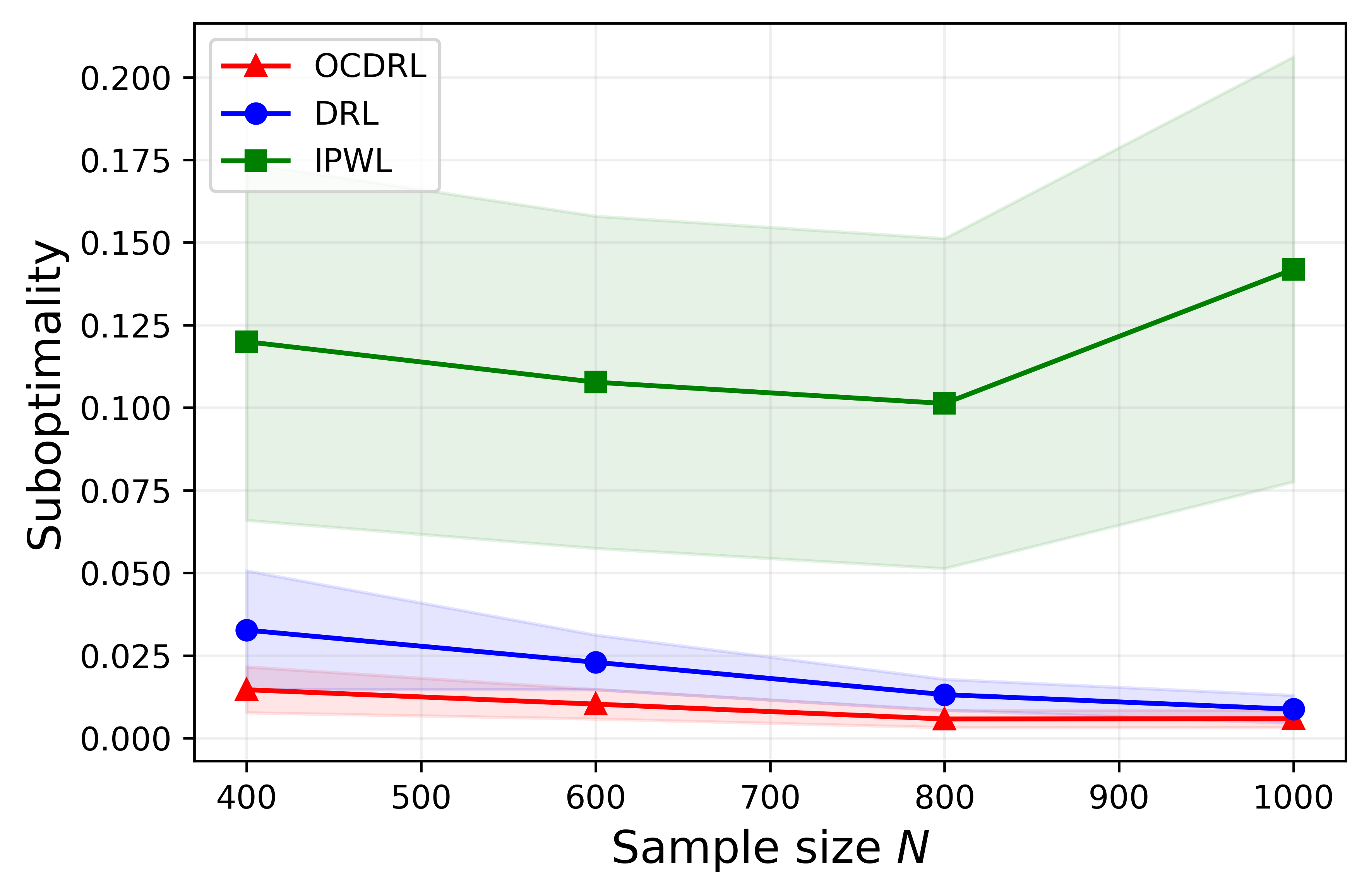
Refer to caption
Figure 2: Out-of-Sample Suboptimality Gaps

We further visualize the behavior of the three algorithms in Figure 3, which provides additional evidence that high variance in policy evaluation can mislead policy learning algorithms. Recall that in the experimental design, the suboptimal and worst treatments are assigned very small propensity scores, which substantially inflate the variance of policy value estimates produced by the DR and IPW estimators. As a consequence, DRL and IPWL tend to select suboptimal and worst treatments more frequently than OCDRL, driven by spuriously inflated policy value estimates. In contrast, OCDRL effectively mitigates the high variance issue via weight clipping. Moreover, the empirical results indicate that the bias introduced by variance reduction is small enough, since it does not cause OCDRL to favor suboptimal or worst treatments more frequently than the benchmark algorithms.

Refer to caption
Figure 3: Treatment Selection Behavior of Different Algorithms

7.3 Assessment with Real-World Data: Targeting Policy for Insurance Products

We further evaluate the proposed policy learning framework using a real-world data set from a randomized controlled trial (RCT) conducted by cai2015social, which studies the heterogeneous effects of information sessions on farmers’ weather insurance take-up rates.The data set is available at: Dean Eckles and Jeremy Yang. Counterfactual policy learning in 15.838. https://kaggle.com/competitions/mitsloancounterfactualpolicy, 2019. Kaggle. This data set is ideal for performance evaluation because it is collected from an RCT, which implies that, (i) the assumptions on the offline data (Assumption 2.1) are naturally satisfied, and (ii) the known treatment probabilities (propensity scores) enable unbiased estimation of counterfactual rewards, providing a reliable measure of performance. In the experiment, households were randomly assigned to an intensive information session that provided detailed explanations of the expected benefits of the insurance product. The treatment is binary, with J=1J=1 indicating assignment to the intensive information session. Households’ insurance purchase decisions were recorded, along with a rich set of covariates capturing household-level heterogeneity. Our policy learning problem is motivated by the observation that individuals respond heterogeneously to insurance information sessions/advertising campaigns (see, e.g., aizawa2018advertising, cai2015social, cole2011prices, shapiro2020advertising), which calls for the design of a cost-effective targeting policy that delivers information sessions to individuals who are most likely to be influenced by such interventions. We assume that the expected profit from selling insurance to a household is 100 RMB, while delivering an intensive information session incurs a cost of 15 RMB per household. This defines the insurer’s reward function: Y=100​R−15​DY=100R-15D, where R,D∈{0,1}R,D\in\{0,1\} denote the purchase decision and the treatment received, respectively. We consider a targeting policy from the linear policy class that depends on three covariates: the household’s risk aversion, perceived probability of natural disasters in the following year, and share of rice income in total income. Such information can often be obtained by insurance companies through customer surveys. See, e.g., a consumer survey conducted by Swiss Re (one of the world’s leading providers of insurance): https://www.swissre.com/reinsurance/insights/asia-protection-gap-consumer-survey.html. We also refer interested readers to cai2015social for further details on the measurement of these covariates. We split the data set (N=4,715N=4{,}715) into a training set and an evaluation set in a 1:11{:}1 ratio. Policies learned from the training set by our proposed OCDRL and the benchmark methods are evaluated on the evaluation set, where counterfactual rewards are estimated using the IPW estimator, which provides an unbiased estimate of the mean reward given known treatment assignment probabilities. As shown in Table 2, the policy learned by our proposed OCDRL achieves higher expected rewards than the benchmark methods. We also note that, although our algorithm requires more computation time than DRL, which shares a similar problem structure, this additional effort arises from optimizing the clipping threshold to achieve improved statistical performance.

Table 2: Rewards and Computation Time of Different Algorithms
Method OCDRL DRL IPWL
Reward 46.71 46.12 38.87
Time 1.39s 0.58s 1.91s

Note. All learning algorithms use the PIP as the embedded computation method. Reward is measured by RMB.

We close this section by discussing the managerial implications of the targeting policy learned by our proposed OCDRL (a visualization of the policy can be found in Figure 4 in the online appendix). First, households’ perceived probability of a disaster is a dominant covariate influencing the assignment of information sessions. All households targeted by our learned policy have a perceived disaster probability of at least 75%75\%. Second, the covariates interact in the assignment rule. For example, conditional on a high perceived disaster probability, households with lower risk aversion tend to be treated primarily when the share of rice income is high, but risk-averse households should be assigned even when the share of rice income is low.

8 Concluding Remarks

In this paper, we systematically develop an offline policy learning framework based on a weight-clipping estimator, with the desire for mitigating the adverse impact of high variance in policy evaluation on downstream policy optimization. Focusing on a linear policy class, we address the optimization challenges arising from the associated bilevel and discontinuous objective by (i) explicitly characterizing the optimal weight-clipping threshold as the minimizer of MSE in policy evaluation, and (ii) reformulating the policy optimization problem as a Heaviside composite optimization problem. We further tackle the computational challenges by developing a progressive integer programming algorithm, adapted from fang2025treatment, which offers substantial computational advantages over conventional MIP approaches. The success of our optimization and computational approaches renders weight-clipping-based policy learning practically implementable at scale. We also establish a theoretical suboptimality guarantee for the proposed framework, which reveals how policy learning performance benefits from the optimized choice of the weight-clipping threshold.

References

\ECSwitch\OneAndAHalfSpacedXI\ECHead

Online Appendices

9 Proofs of Statements in Section 2

9.1 Proof of Proposition 2.1

Proof. Note that when condition on XsX^{s}, μ^​(Xs,g​(Xs))\widehat{\mu}(X^{s},g(X^{s})) is a constant and does not contribute to the variance, so it is omitted. For notational simplicity, we drop the subscripts and superscripts ss.

Var​(Γ^DR​(g)∣X)=1e​(X,g​(X))2⋅Var​(𝟏​{g​(X)=D}​(Y−μ^​(X,g​(X)))∣X)\displaystyle\mathrm{Var}(\widehat{\Gamma}^{\mathrm{DR}}(g)\mid X)=\frac{1}{e(X,g(X))^{2}}\cdot\mathrm{Var}({\bf 1}\{g(X)=D\}(Y-\widehat{\mu}(X,g(X)))\mid X)
=1e​(X,g​(X))2⋅(𝔼​[𝟏​{g​(X)=D}2​(Y−μ^​(X,g​(X)))2∣X]−𝔼​[𝟏​{g​(X)=D}​(Y−μ^​(X,g​(X)))∣X]2).\displaystyle=\frac{1}{e(X,g(X))^{2}}\cdot\left(\mathbb{E}[{\bf 1}\{g(X)=D\}^{2}(Y-\widehat{\mu}(X,g(X)))^{2}\mid X]-\mathbb{E}[{\bf 1}\{g(X)=D\}(Y-\widehat{\mu}(X,g(X)))\mid X]^{2}\right). (15)

To rewrite the above equation, we note that

𝔼​[𝟏​{g​(X)=D}2​(Y−μ^​(X,g​(X)))2∣X]\displaystyle\mathbb{E}[{\bf 1}\{g(X)=D\}^{2}(Y-\widehat{\mu}(X,g(X)))^{2}\mid X]
=𝔼​[𝟏​{g​(X)=D}​(Y−μ^​(X,g​(X)))2∣X]\displaystyle=\mathbb{E}[{\bf 1}\{g(X)=D\}(Y-\widehat{\mu}(X,g(X)))^{2}\mid X]
=e​(X,g​(X))⋅𝔼​[Y2−2​Y​μ^​(X,g​(X))+μ^​(X,g​(X))2∣X]\displaystyle=e(X,g(X))\cdot\mathbb{E}[Y^{2}-2Y\widehat{\mu}(X,g(X))+\widehat{\mu}(X,g(X))^{2}\mid X]
=e​(X,g​(X))⋅(𝔼​[Y2∣X]−2​𝔼​[Y∣X]​μ^​(X,g​(X))+μ^​(X,g​(X))2).\displaystyle=e(X,g(X))\cdot(\mathbb{E}[Y^{2}\mid X]-2\mathbb{E}[Y\mid X]\widehat{\mu}(X,g(X))+\widehat{\mu}(X,g(X))^{2}). (16)

In addition,

e​(X,g​(X))2⋅(𝔼​[Y∣X]−μ^​(X,g​(X)))2=e​(X,g​(X))2⋅(𝔼​[Y∣X]2−2​𝔼​[Y∣X]​μ^​(X,g​(X))+μ^​(X,g​(X))2).\displaystyle e(X,g(X))^{2}\cdot(\mathbb{E}[Y\mid X]-\widehat{\mu}(X,g(X)))^{2}=e(X,g(X))^{2}\cdot(\mathbb{E}[Y\mid X]^{2}-2\mathbb{E}[Y\mid X]\widehat{\mu}(X,g(X))+\widehat{\mu}(X,g(X))^{2}). (17)

Therefore, the inner conditional variance term in Equation (15) can be rewritten as

𝔼​[𝟏​{g​(X)=D}2​(Y−μ^​(X,g​(X)))2∣X]−𝔼​[𝟏​{g​(X)=j}​(Y−μ^​(X,g​(X)))∣X]2\displaystyle\mathbb{E}[{\bf 1}\{g(X)=D\}^{2}(Y-\widehat{\mu}(X,g(X)))^{2}\mid X]-\mathbb{E}[{\bf 1}\{g(X)=j\}(Y-\widehat{\mu}(X,g(X)))\mid X]^{2}
=e​(X,g​(X))⋅(𝔼​[Y2∣X]−2​𝔼​[Y∣X]​μ^+μ^2)−e​(X,g​(X))2⋅(𝔼​[Y∣X]2−2​𝔼​[Y∣X]​μ^​(X,g​(X))+μ^​(X,g​(X))2)\displaystyle=e(X,g(X))\cdot(\mathbb{E}[Y^{2}\mid X]-2\mathbb{E}[Y\mid X]\widehat{\mu}+\widehat{\mu}^{2})-e(X,g(X))^{2}\cdot(\mathbb{E}[Y\mid X]^{2}-2\mathbb{E}[Y\mid X]\widehat{\mu}(X,g(X))+\widehat{\mu}(X,g(X))^{2})
=e​(X,g​(X))⋅(𝔼​[Y2∣X]−𝔼​[Y∣X]2+𝔼​[Y∣X]2−2​𝔼​[Y∣X]​μ^​(X,g​(X))+μ^​(X,g​(X))2)\displaystyle=e(X,g(X))\cdot(\mathbb{E}[Y^{2}\mid X]-\mathbb{E}[Y\mid X]^{2}+\mathbb{E}[Y\mid X]^{2}-2\mathbb{E}[Y\mid X]\widehat{\mu}(X,g(X))+\widehat{\mu}(X,g(X))^{2})
−e​(X,g​(X))2⋅(𝔼​[Y∣X]2−2​𝔼​[Y∣X]​μ^​(X,g​(X))+μ^​(X,g​(X))2)\displaystyle~~~~-e(X,g(X))^{2}\cdot(\mathbb{E}[Y\mid X]^{2}-2\mathbb{E}[Y\mid X]\widehat{\mu}(X,g(X))+\widehat{\mu}(X,g(X))^{2})
=e​(X,g​(X))​Var​(Y∣X)+e​(X,g​(X))​(1−e​(X,g​(X)))​(𝔼​[Y∣X]−μ^​(X,g​(X)))2\displaystyle=e(X,g(X))\mathrm{Var}(Y\mid X)+e(X,g(X))(1-e(X,g(X)))(\mathbb{E}[Y\mid X]-\widehat{\mu}(X,g(X)))^{2} (18)

Finally, plugging (18) into (15) to obtain

Var​(Γ^​(g)∣X)=1e​(X,g​(X))​Var​(Y∣X)+(1e​(X,g​(X))−1)⋅(𝔼​[Y∣X]−μ^​(X,g​(X)))2.\displaystyle\mathrm{Var}(\widehat{\Gamma}(g)\mid X)=\frac{1}{e(X,g(X))}\mathrm{Var}(Y\mid X)+\left(\frac{1}{e(X,g(X))}-1\right)\cdot(\mathbb{E}[Y\mid X]-\widehat{\mu}(X,g(X)))^{2}. (19)

By the assumption that Var​(Y∣X)≤L′\mathrm{Var}(Y\mid X)\leq L^{\prime}, we can lower bound (19) by

L′e​(X,g​(X)).\displaystyle\frac{L^{\prime}}{e(X,g(X))}.

By the assumption that Var​(Y∣X)≤U′\mathrm{Var}(Y\mid X)\leq U^{\prime} and (𝔼​[Y∣X]−μ^​(X,g​(X)))2≤M2(\mathbb{E}[Y\mid X]-\widehat{\mu}(X,g(X)))^{2}\leq M^{2} (which follows from Assumption 2.1(C)), we can upper bound (19) by

L′+M2e​(X,g​(X)).\displaystyle\frac{L^{\prime}+M^{2}}{e(X,g(X))}.

Letting L=L′L=L^{\prime} and U=U′+M2U=U^{\prime}+M^{2} to yield the desired result. \halmos

10 Proofs of Statements in Section 3

10.1 Proof of Proposition 3.2

Proof 10.1

Proof. First, for any policy g∈𝒢g\in\mathcal{G}, following the routine bias-variance decomposition, we have

𝔼​[(Ψ^CDR​(g)−Ψ​(g))2]=𝔼​[Ψ^CDR​(g)−Ψ​(g)]2⏟Bias2+Var​(Ψ^CDR​(g))⏟Variance.\displaystyle\mathbb{E}\left[(\widehat{\Psi}^{\mathrm{CDR}}(g)-\Psi(g))^{2}\right]=\underbrace{\mathbb{E}\left[\widehat{\Psi}^{\mathrm{CDR}}(g)-\Psi(g)\right]^{2}}_{\mathrm{Bias}^{2}}+\underbrace{\mathrm{Var}\left(\widehat{\Psi}^{\mathrm{CDR}}(g)\right)}_{\mathrm{Variance}}.

Note that for any given policy g∈𝒢g\in\mathcal{G}, the bias term is only incurred when e​(X,g​(X))−1>τe(X,g(X))^{-1}>\tau; otherwise, the CDR estimator switches to the DR estimator, which enjoys unbiasedness given that the propensity score is known. To see this, we show that the bias term can be decomposed as

𝔼​[Ψ^CDR​(g)−Ψ​(g)]\displaystyle\mathbb{E}\left[\widehat{\Psi}^{\mathrm{CDR}}(g)-\Psi(g)\right]
=𝔼​[(μ^​(X,g​(X))−μ​(X,g​(X)))⋅𝟏​{1e​(X,g​(X))>τ}]⏟(i)\displaystyle\quad=\underbrace{\mathbb{E}\left[(\widehat{\mu}(X,g(X))-\mu(X,g(X)))\cdot{\bf 1}\left\{\frac{1}{e(X,g(X))}>\tau\right\}\right]}_{\mathrm{(i)}}
+𝔼​[(μ^​(X,g​(X))+𝟏​{g​(X)=D}e​(X,g​(X))​(Y−μ^​(X,g​(X)))−μ​(X,g​(X)))⋅𝟏​{1e​(X,g​(X))≤τ}]⏟(ii).\displaystyle\quad\quad+\underbrace{\mathbb{E}\left[\left(\widehat{\mu}(X,g(X))+\frac{{\bf 1}\{g(X)=D\}}{e(X,g(X))}(Y-\widehat{\mu}(X,g(X)))-\mu(X,g(X))\right)\cdot{\bf 1}\left\{\frac{1}{e(X,g(X))}\leq\tau\right\}\right]}_{\mathrm{(ii)}}.

Term (i) can be upper bounded using the bounded reward assumption (Assumption 2.1(C)), such that

(i)≤M⋅𝔼​[𝟏​{1e​(X,g​(X))>τ}].\displaystyle(i)\leq M\cdot\mathbb{E}\left[{\bf 1}\left\{\frac{1}{e(X,g(X))}>\tau\right\}\right].

As for term (ii), we show that it is unbiased:

𝔼​[𝔼​[(μ^​(X,g​(X))+𝟏​{g​(X)=D}e​(X,g​(X))​(Y−μ^​(X,g​(X)))−μ​(X,g​(X)))|X]⋅𝟏​{1e​(X,g​(X))≤τ}]\displaystyle\mathbb{E}\left[\mathbb{E}\left[\left(\widehat{\mu}(X,g(X))+\frac{{\bf 1}\{g(X)=D\}}{e(X,g(X))}(Y-\widehat{\mu}(X,g(X)))-\mu(X,g(X))\right)\bigg|X\right]\cdot{\bf 1}\left\{\frac{1}{e(X,g(X))}\leq\tau\right\}\right]
=𝔼​[(μ^​(X,g​(X))+e​(X,g​(X))e​(X,g​(X))​(μ​(X,g​(X))−μ^​(X,g​(X)))−μ​(X,g​(X)))⋅𝟏​{1e​(X,g​(X))≤τ}]\displaystyle=\mathbb{E}\left[\left(\widehat{\mu}(X,g(X))+\frac{e(X,g(X))}{e(X,g(X))}(\mu(X,g(X))-\widehat{\mu}(X,g(X)))-\mu(X,g(X))\right)\cdot{\bf 1}\left\{\frac{1}{e(X,g(X))}\leq\tau\right\}\right]
=0,\displaystyle=0,

where the second equality is due to the definition of propensity score, namely, e​(X,g​(X))=ℙ(g​(X)∣X)e(X,g(X))=\operatorname*{\mathbb{P}}(g(X)\mid X). Therefore, the squared bias term is bounded as follows

𝔼​[Ψ^CDR​(g)−Ψ​(g)]2≤M2⋅𝔼​[𝟏​{1e​(X,g​(X))>τ}]2.\displaystyle\mathbb{E}\left[\widehat{\Psi}^{\mathrm{CDR}}(g)-\Psi(g)\right]^{2}\leq M^{2}\cdot\mathbb{E}\left[{\bf 1}\left\{\frac{1}{e(X,g(X))}>\tau\right\}\right]^{2}.

Next, we upper bound the variance. The analysis starts from the fact that Var​(A+B)≤2​V​a​r​(A)+2​V​a​r​(B)\mathrm{Var}(A+B)\leq 2\mathrm{Var}(A)+2\mathrm{Var}(B), where AA and BB are not independent.

Var​(Ψ^CDR​(g))\displaystyle\mathrm{Var}\left(\widehat{\Psi}^{\mathrm{CDR}}(g)\right)
≤2​V​a​r​(1N​∑s=1Nμ^​(Xs,g​(Xs)))⏟(iii)+2​V​a​r​(1N​∑s=1N𝟏​{g​(Xs)=Ds}e​(Xs,g​(Xs))⋅𝟏​{1e​(Xs,g​(Xs))≤τ}​(Ys−μ^​(Xs,g​(Xs))))⏟(iv).\displaystyle\qquad\leq\underbrace{2\mathrm{Var}\left(\frac{1}{N}\sum_{s=1}^{N}\widehat{\mu}(X^{s},g(X^{s}))\right)}_{\mathrm{(iii)}}+\underbrace{2\mathrm{Var}\left(\frac{1}{N}\sum_{s=1}^{N}\frac{{\bf 1}\{g(X^{s})=D_{s}\}}{e(X^{s},g(X^{s}))}\cdot{\bf 1}\left\{\frac{1}{e(X^{s},g(X^{s}))}\leq\tau\right\}(Y_{s}-\widehat{\mu}(X^{s},g(X^{s})))\right)}_{\mathrm{(iv)}}.

Term (iii) can be bounded as follows.

2​V​a​r​(1N​∑s=1Nμ^​(Xs,g​(Xs)))≤2N​𝔼​[μ^​(X,g​(X))2]≤2N​M2,\displaystyle 2\mathrm{Var}\left(\frac{1}{N}\sum_{s=1}^{N}\widehat{\mu}(X^{s},g(X^{s}))\right)\leq\frac{2}{N}\mathbb{E}\left[\widehat{\mu}(X,g(X))^{2}\right]\leq\frac{2}{N}M^{2},

where the first inequality uses the fact that Var​(A)=𝔼​[A2]−𝔼​[A]2≤𝔼​[A2]\mathrm{Var}(A)=\mathbb{E}[A^{2}]-\mathbb{E}[A]^{2}\leq\mathbb{E}[A^{2}] and the final inequality uses Assumption 2.1(C). Similarly, term (iv) can be bounded by

2​V​a​r​(1N​∑s=1N𝟏​{g​(Xs)=Ds}e​(Xs,g​(Xs))⋅𝟏​{1e​(Xs,g​(Xs))≤τ}​(Ys−μ^​(Xs,g​(Xs))))\displaystyle 2\mathrm{Var}\left(\frac{1}{N}\sum_{s=1}^{N}\frac{{\bf 1}\{g(X^{s})=D_{s}\}}{e(X^{s},g(X^{s}))}\cdot{\bf 1}\left\{\frac{1}{e(X^{s},g(X^{s}))}\leq\tau\right\}(Y_{s}-\widehat{\mu}(X^{s},g(X^{s})))\right)
≤2N​𝔼​[𝟏​{g​(X)=D}e​(X,g​(X))2​(Y−μ^​(X,g​(X)))2⋅𝟏​{1e​(X,g​(X))≤τ}]\displaystyle\quad\leq\frac{2}{N}\mathbb{E}\left[\frac{{\bf 1}\{g(X)=D\}}{e(X,g(X))^{2}}(Y-\widehat{\mu}(X,g(X)))^{2}\cdot{\bf 1}\left\{\frac{1}{e(X,g(X))}\leq\tau\right\}\right]
≤2​M2N​𝔼​[𝟏​{g​(X)=D}e​(X,g​(X))2⋅𝟏​{1e​(X,g​(X))≤τ}].\displaystyle\quad\leq\frac{2M^{2}}{N}\mathbb{E}\left[\frac{{\bf 1}\{g(X)=D\}}{e(X,g(X))^{2}}\cdot{\bf 1}\left\{\frac{1}{e(X,g(X))}\leq\tau\right\}\right].

Putting pieces together to yield

𝔼​[(Ψ^CDR​(g)−Ψ​(g))2]\displaystyle\mathbb{E}\left[(\widehat{\Psi}^{\mathrm{CDR}}(g)-\Psi(g))^{2}\right]
≤M2⋅𝔼​[𝟏​{1e​(X,g​(X))>τ}]2+2​M2N​𝔼​[𝟏​{g​(X)=D}e​(X,g​(X))2⋅𝟏​{1e​(X,g​(X))≤τ}]+2N​M2.\halmos\displaystyle\qquad\leq M^{2}\cdot\mathbb{E}\left[{\bf 1}\left\{\frac{1}{e(X,g(X))}>\tau\right\}\right]^{2}+\frac{2M^{2}}{N}\mathbb{E}\left[\frac{{\bf 1}\{g(X)=D\}}{e(X,g(X))^{2}}\cdot{\bf 1}\left\{\frac{1}{e(X,g(X))}\leq\tau\right\}\right]+\frac{2}{N}M^{2}.\halmos

11 Proofs of Statements in Section 4

11.1 Proof of Proposition 4.1

Recall that

θ~​(τ​(g);g)={Φm​(g) if ​C(m−1)≤τ​(g)<C(m), for ​m=1,2,…,N,ΦN+1​(g)≡0 if ​τ​(g)≥C(N),\widetilde{\theta}(\tau(g);g)=\begin{cases}\Phi_{m}(g)&\mbox{ if }C_{(m-1)}\leq\tau(g)<C_{(m)},\quad\mbox{ for }m=1,2,\ldots,N,\\ \Phi_{N+1}(g)\equiv 0&\mbox{ if }\tau(g)\geq C_{(N)},\end{cases}

which implies that the expression of τ^​(g)\widehat{\tau}(g) can be explicitly computed as follows,

τ^​(g)={C(0)if ​Φ1​(g)≤min⁡{Φi​(g):i=2,…,N+1},C(m)if ​{Φm+1​(g)<min⁡{Φi​(g):i=1,…,m}, and ​Φm+1​(g)≤min⁡{Φi​(g):i=m+2,…,N+1}}​ for ​m=1,…,N−1,C(N)if ​ΦN+1​(g)<min⁡{Φi​(g):i=1,2,…,N}.\widehat{\tau}(g)=\begin{cases}C_{(0)}&\mbox{if }\Phi_{1}(g)\leq\min\{\Phi_{i}(g):i=2,\ldots,N+1\},\\ C_{(m)}&\mbox{if }\left\{\begin{array}[]{l}\Phi_{m+1}(g)<\min\{\Phi_{i}(g):i=1,\ldots,m\},\\ \mbox{ and }\Phi_{m+1}(g)\leq\min\{\Phi_{i}(g):i=m+2,\ldots,N+1\}\end{array}\right\}\mbox{ for }m=1,\ldots,N-1,\\ C_{(N)}&\mbox{if }\Phi_{N+1}(g)<\min\{\Phi_{i}(g):i=1,2,\ldots,N\}.\\ \end{cases}

Based on the above expression of τ^​(g)\widehat{\tau}(g), in general, we have

τ^​(g)=C(0)⋅𝟏[0,∞)​(min2≤t≤N+1⁡Φ¯t,1​(g))+∑m=1N−1C(m)⋅𝟏[0,∞)​(minm+2≤t≤N+1⁡Φ¯t,m+1​(g))⋅𝟏(0,∞)​(min1≤t≤m⁡Φ¯t,m+1​(g))+C(N)⋅𝟏(0,∞)​(min1≤t≤N⁡Φ¯t,N+1​(g)).\begin{array}[]{lll}\widehat{\tau}(g)&=&C_{(0)}\cdot\displaystyle{{\bf 1}_{[0,\infty)}}\left(\min_{2\leq t\leq N+1}\bar{\Phi}_{t,1}(g)\right)\\[7.22743pt] &&+\displaystyle{\sum_{m=1}^{N-1}}C_{(m)}\cdot{\bf 1}_{[0,\infty)}\left(\min_{m+2\leq t\leq N+1}\bar{\Phi}_{t,m+1}(g)\right)\cdot\displaystyle{{\bf 1}_{(0,\infty)}}\left(\min_{1\leq t\leq m}\bar{\Phi}_{t,m+1}(g)\right)\\[7.22743pt] &&+C_{(N)}\cdot\displaystyle{{\bf 1}_{(0,\infty)}}\left(\min_{1\leq t\leq N}\bar{\Phi}_{t,N+1}(g)\right).\end{array}

Furthermore, under Assumption 4.1, the above expression simplifies to

τ^​(g)=∑m=0NC(m)⋅𝟏(0,∞)​(mint∈[N+1],t≠m+1⁡Φt​(g)−Φm+1​(g)).​\halmos\begin{array}[]{ll}\widehat{\tau}(g)=\displaystyle{\sum_{m=0}^{N}}\,C_{(m)}\cdot\displaystyle{{\bf 1}_{(0,\infty)}}\left(\min_{t\in[N+1],t\neq m+1}\Phi_{t}(g)-\Phi_{m+1}(g)\right).\end{array}\halmos

11.2 Proof of Proposition 4.2

We prove this proposition by contradiction. Suppose there exists an optimal m′≠N+1m^{\prime}\neq N+1 that gives the minimum Φm′​(g)\Phi_{m^{\prime}}(g), such that 2​φ~(m′)<2​(N−m′)+12\tilde{\varphi}_{(m^{\prime})}<2(N-m^{\prime})+1. Given that φ~(m′)≥φ(m′)​(g)\tilde{\varphi}_{(m^{\prime})}\geq\varphi_{(m^{\prime})}(g), we have φ(m′)​(g)≤2​φ~(m′)<2​(N−m′)+1\varphi_{(m^{\prime})}(g)\leq 2\tilde{\varphi}_{(m^{\prime})}<2(N-m^{\prime})+1, which implies that 2​(N−m′)+1−2​φ(m′)​(g)>02(N-m^{\prime})+1-2\varphi_{(m^{\prime})}(g)>0. By the definition of Φm​(g)\Phi_{m}(g), we know that Φm′+1​(g)<Φm′​(g)\Phi_{m^{\prime}+1}(g)<\Phi_{m^{\prime}}(g), contradicting m′m^{\prime} achieves the minimum.\Halmos

11.3 Proof of Proposition 4.3

Under the pruning strategy, the explicit optimal solution τ^​(g)\widehat{\tau}(g) can be rewritten as

τ^​(g)={C(m∗−1)if ​Φm∗​(g)≤min⁡{Φi​(g):i≥m∗+1},C(m)if ​{Φm+1​(g)<min⁡{Φi​(g):m≥i≥m∗}, and Φm+1​(g)≤min⁡{Φi​(g):N+1≥i≥m+2}}​ for ​N−1≥m≥m∗,C(N)if ​m∗=N​ or ​ΦN+1​(g)<min⁡{Φi​(g):N≥i≥m∗}.\widehat{\tau}(g)=\begin{cases}{C}_{(m^{*}-1)}&\mbox{if }{\Phi}_{m^{*}}(g)\leq\min\{{\Phi}_{i}(g):i\geq m^{*}+1\},\\ {C}_{(m)}&\mbox{if }\left\{\begin{array}[]{l}{\Phi}_{m+1}(g)<\min\{{\Phi}_{i}(g):m\geq i\geq m^{*}\},\mbox{ and }\\ {\Phi}_{m+1}(g)\leq\min\{{\Phi}_{i}(g):N+1\geq i\geq m+2\}\end{array}\right\}\mbox{ for }N-1\geq m\geq m^{*},\\ {C}_{({N})}&\mbox{if }m^{*}=N\mbox{ or }{\Phi}_{{N}+1}(g)<\min\{{\Phi}_{i}(g):N\geq i\geq m^{*}\}.\\ \end{cases}

Furthermore, Assumption 4.1 guarantees that the distinct values of {Φm∗​(g)}\{\Phi_{m}^{*}(g)\} for any g∈𝒢g\in\mathcal{G}. \halmos

11.4 Proof of Proposition 6

Proof 11.1

Proof. (A) We first observe that for any scalar t∗≠0t_{*}\neq 0, there exist a scalar ε∗>0\varepsilon_{*}>0 and a neighborhood 𝒯∗{\cal T}_{*} of t∗t_{*} such that 𝟏(−ε,∞)​(t)= 1[ 0,∞)​(t∗){\bf 1}_{(\,-\varepsilon,\infty)}(t)\,=\,{\bf 1}_{[\,0,\infty)}(t_{*}) and 𝟏[ε,∞)​(t)= 1( 0,∞)​(t∗){\bf 1}_{[\,\varepsilon,\infty)}(t)\,=\,{\bf 1}_{(\,0,\infty)}(t_{*}) for any (t,ε)∈𝒯∗×(0,ε∗].(t,\varepsilon)\in{\cal T}_{*}\times(0,\varepsilon_{*}]. Then, for any ξ∈Ξ\xi\in\Xi with min1≤i≤j−1⁡hj,i​(ξ,𝛃¯)≠0\min_{1\leq i\leq j-1}h_{j,i}(\xi,\overline{\bm{\beta}})\neq 0, there exist a scalar ε¯1>0\bar{\varepsilon}_{1}>0 and a neighborhood 𝒩1{\cal N}_{1} of 𝛃¯\overline{\bm{\beta}} such that for any 𝛃∈𝒩1\bm{\beta}\in{\cal N}_{1} and 0<ε≤ε¯10<\varepsilon\leq\bar{\varepsilon}_{1},

𝟏( 0,∞)​(min1≤i≤j−1⁡hj,i​(ξ,𝜷))=𝟏[ε,∞)​(min1≤i≤j−1⁡hj,i​(ξ,𝜷))=𝟏[ 0,∞)​(min1≤i≤j−1⁡hj,i​(ξ,𝜷)−ε),{\bf 1}_{(\,0,\infty)}\left(\min_{1\leq i\leq j-1}h_{j,i}(\xi,\bm{\beta})\right)={\bf 1}_{[\,\varepsilon,\infty)}\left(\min_{1\leq i\leq j-1}h_{j,i}(\xi,\bm{\beta})\right)={\bf 1}_{[\,0,\infty)}\left(\min_{1\leq i\leq j-1}h_{j,i}(\xi,\bm{\beta})-\,\varepsilon\right),

which thus yields the claimed statement. (B) For the local maximizer 𝛃¯\overline{\bm{\beta}} to the optimization problem (11), based on statement (A), there exist ε>0\varepsilon>0 and a neighborhood 𝒩\mathcal{N} of 𝛃¯\overline{\bm{\beta}} such that for any 𝛃∈𝒩{\bm{\beta}}\in\mathcal{N}, Ψ^ε​(𝛃)≤Ψ^HSC​(𝛃)≤Ψ^HSC​(𝛃¯)=Ψ^ε​(𝛃¯)\widehat{\Psi}_{\varepsilon}(\bm{\beta})\leq\widehat{\Psi}_{\rm HSC}(\bm{\beta})\leq\widehat{\Psi}_{\rm HSC}(\overline{\bm{\beta}})=\widehat{\Psi}_{\varepsilon}(\overline{\bm{\beta}}). Thus 𝛃¯\overline{\bm{\beta}} is a local maximizer of (13). (C) For the local maximizer 𝛃¯\overline{\bm{\beta}} of (13), under the sign-invariance condition, there exist ε\varepsilon and a neighborhood 𝒩\mathcal{N} of 𝛃¯\overline{\bm{\beta}} such that for any 𝛃∈𝒩{\bm{\beta}}\in\mathcal{N}, ∀j×s∈{(ℓ,t):ℓ∈[J],min1≤i≤ℓ−1⁡hℓ,i​(Xt,𝛃¯)=0}\forall j\times s\in\{(\ell,t):\ell\in[J],\min_{1\leq i\leq\ell-1}h_{\ell,i}(X^{t},\overline{\bm{\beta}})=0\},

𝟏[ 0,∞)​(hj1​(Xs,𝜷;ε))=𝟏( 0,∞)​(min1≤i≤j−1⁡hj,i​(Xs,𝜷))×𝟏[ 0,∞)​(minj+1≤i≤J⁡hj,i​(Xs,𝜷)),\begin{array}[]{ll}{{\bf 1}_{[\,0,\infty)}(h^{1}_{j}(X^{s},\bm{\beta};\varepsilon))}={\bf 1}_{(\,0,\infty)}\left(\min_{1\leq i\leq j-1}h_{j,i}(X^{s},\bm{\beta})\right)\times{\bf 1}_{[\,0,\infty)}\left(\min_{j+1\leq i\leq J}h_{j,i}(X^{s},\bm{\beta})\right),\end{array}

and for all s​ satisfying ​minDs+1≤i≤J⁡hDs,i​(Xs,𝛃¯)=0s\mbox{ satisfying }\min_{D_{s}+1\leq i\leq J}h_{D_{s},i}(X^{s},\overline{\bm{\beta}})=0,

𝟏( 0,∞)​(min1≤i≤Ds−1⁡hDs,i​(Xs,𝜷))×𝟏[ 0,∞)​(minj+1≤i≤J⁡hDs,i​(Xs,𝜷))=𝟏( 0,∞)​(hDs2​(Xs,𝜷;ε)),\begin{array}[]{ll}{\bf 1}_{(\,0,\infty)}\left(\min_{1\leq i\leq D_{s}-1}h_{D_{s},i}(X^{s},\bm{\beta})\right)\times{\bf 1}_{[\,0,\infty)}\left(\min_{j+1\leq i\leq J}h_{D_{s},i}(X^{s},\bm{\beta})\right)={{\bf 1}_{(\,0,\infty)}(h^{2}_{D_{s}}(X^{s},\bm{\beta};\varepsilon))},\end{array}

Based on (12), it is then not difficult to see that for any 𝛃∈𝒩{\bm{\beta}}\in\mathcal{N},

Ψ^HSC​(𝜷¯)≥Ψ^ε​(𝜷¯)≥Ψ^ε​(𝜷)=Ψ^HSC​(𝜷),\widehat{\Psi}_{\rm HSC}(\overline{\bm{\beta}})\geq\widehat{\Psi}_{\varepsilon}(\overline{\bm{\beta}})\geq\widehat{\Psi}_{\varepsilon}({\bm{\beta}})=\widehat{\Psi}_{\rm HSC}({\bm{\beta}}),

where the last equality is obtained by the above analysis under the sign-invariance condition. \halmos

12 Proofs of Statements in Section 6

12.1 Proof of Theorem 6.1

We begin by introducing a standard measure of policy class complexity, which will be used to characterize the performance of policy learning algorithms.

Definition 12.1 (Natarajan dimension)

Given a JJ-action policy class 𝒢={}∈𝒢:𝒳→[𝒥]}\cal{G}=\{g\in\mathcal{G}:\cal{X}\to[J]\}, we say a set of mm points {ξ1,⋯,ξm}\{\xi_{1},\cdots,\xi_{m}\} is shattered by 𝒢\cal{G} if there exist two functions f1,f2:{ξ1,⋯,ξm}↦[J]f_{1},f_{2}:\{\xi_{1},\cdots,\xi_{m}\}\mapsto[J], such that

  • (i)

    For any k∈[m]k\in[m], f1​(ξj)≠f2​(ξj)f_{1}(\xi_{j})\neq f_{2}(\xi_{j});

  • (ii)

    For any subset S⊆[m]S\subseteq[m], there exists some g∈𝒢g\in\cal{G}, such that g​(ξk)=f1​(ξk)g(\xi_{k})=f_{1}(\xi_{k}) for all k∈Sk\in S and g​(ξk)=f2​(ξk)g(\xi_{k})=f_{2}(\xi_{k}) for all k∉Sk\notin S.

The Natarajan dimension of 𝒢\mathcal{G}, defined as 𝒩⌈⟩⇕​(𝒢)\cal{N}_{\mathrm{dim}}(\mathcal{G}), is the largest size of a set of points shattered by 𝒢\mathcal{G}.

In particular, 𝒩⌈⟩⇕​(𝒢ℒ​𝒫​𝒞)≤|𝒥|​(√+∞)\cal{N}_{\mathrm{dim}}(\mathcal{G}_{\rm LPC})\leq|J|(p+1) (shalev2014understanding, Corollary 29.8). Additional notations. For simplicity, we denote Ψ^OCDR​(g)\widehat{\Psi}^{\mathrm{OCDR}}(g) and Γ^sOCDR​(g)\widehat{\Gamma}_{s}^{\mathrm{OCDR}}(g) as Ψ^​(g)\widehat{\Psi}(g) and Γ^s​(g)\widehat{\Gamma}_{s}(g), respectively. We also define

B^​(g,τ^​(g))\displaystyle\widehat{B}(g,\widehat{\tau}(g)) ≜M2N2​((∑s=1N𝟏​{1e​(Xs,g​(Xs))>τ^​(g)})2+∑s=1N𝟏​{Ds=g​(Xs)}e​(Xs,g​(Xs))2​𝟏​{1e​(Xs,g​(Xs))≤τ^​(g)}),\displaystyle\triangleq\frac{M^{2}}{N^{2}}\left(\left(\sum_{s=1}^{N}{\bf 1}\left\{\frac{1}{e(X^{s},g(X^{s}))}>\widehat{\tau}(g)\right\}\right)^{2}+\sum_{s=1}^{N}\frac{{\bf 1}\{D_{s}=g(X^{s})\}}{e(X^{s},g(X^{s}))^{2}}{\bf 1}\left\{\frac{1}{e(X^{s},g(X^{s}))}\leq\widehat{\tau}(g)\right\}\right),
B~​(g,τ^​(g))\displaystyle\widetilde{B}(g,\widehat{\tau}(g)) ≜M2N2​((∑s=1N𝟏​{1e​(Xs,g​(Xs))>τ^​(g)})2+∑s=1N1e​(Xs,g​(Xs))​𝟏​{1e​(Xs,g​(Xs))≤τ^​(g)}),\displaystyle\triangleq\frac{M^{2}}{N^{2}}\left(\left(\sum_{s=1}^{N}{\bf 1}\left\{\frac{1}{e(X^{s},g(X^{s}))}>\widehat{\tau}(g)\right\}\right)^{2}+\sum_{s=1}^{N}\frac{1}{e(X^{s},g(X^{s}))}{\bf 1}\left\{\frac{1}{e(X^{s},g(X^{s}))}\leq\widehat{\tau}(g)\right\}\right),
Δ​(g,τ^​(g))\displaystyle\Delta(g,\widehat{\tau}(g)) ≜M2​(τ^​(g)N)3/2,\displaystyle\triangleq M^{2}\left(\frac{\widehat{\tau}(g)}{N}\right)^{3/2},
A​(g)\displaystyle A(g) ≜max⁡{B^​(g,τ^​(g))1/2,B~​(g,τ^​(g))1/2,Δ​(g,τ^​(g))1/2}.\displaystyle\triangleq\max\left\{\widehat{B}(g,\widehat{\tau}(g))^{1/2},\widetilde{B}(g,\widehat{\tau}(g))^{1/2},\Delta(g,\widehat{\tau}(g))^{1/2}\right\}.

In addition, the following notations will be used to develop the symmetrization technique. For each s∈[N]s\in[N], we let (Ds′,Ys′)(D_{s}^{\prime},Y_{s}^{\prime}) be an independent copy of (Ds,Ys)(D_{s},Y_{s}) conditioned on XsX^{s}, i.e.,

(Ds′,Ys′)⟂(Ds,Ys)∣Xsand(Ds′,Ys′)=d(Ds,Ys)∣Xs.\displaystyle(D_{s}^{\prime},Y_{s}^{\prime})\perp(D_{s},Y_{s})\mid X^{s}\quad\text{and}\quad(D_{s}^{\prime},Y_{s}^{\prime})\stackrel{{\scriptstyle\mathrm{d}}}{{=}}(D_{s},Y_{s})\mid X^{s}.

With such copies, we denote

Γ^s′​(g)\displaystyle\widehat{\Gamma}_{s}^{\prime}(g) =μ^​(Xs,g​(Xs))+𝟏​{Ds′=g​(Xs)}e​(Xs,g​(Xs))​𝟏​{1e​(Xs,g​(Xs))≤τ^​(g)}​(Ys′−μ^​(Xs,g​(Xs))),\displaystyle=\widehat{\mu}(X^{s},g(X^{s}))+\frac{{\bf 1}\{D_{s}^{\prime}=g(X^{s})\}}{e(X^{s},g(X^{s}))}{\bf 1}\left\{\frac{1}{e(X^{s},g(X^{s}))}\leq\widehat{\tau}(g)\right\}(Y_{s}^{\prime}-\widehat{\mu}(X^{s},g(X^{s}))),
B^′​(g,τ^​(g))\displaystyle\widehat{B}^{\prime}(g,\widehat{\tau}(g)) =M2N2​((∑s=1N𝟏​{1e​(Xs,g​(Xs))>τ^​(g)})2+∑s=1N𝟏​{Ds′=g​(Xs)}e​(Xs,g​(Xs))2​𝟏​{1e​(Xs,g​(Xs))≤τ^​(g)})\displaystyle=\frac{M^{2}}{N^{2}}\left(\left(\sum_{s=1}^{N}{\bf 1}\left\{\frac{1}{e(X^{s},g(X^{s}))}>\widehat{\tau}(g)\right\}\right)^{2}+\sum_{s=1}^{N}\frac{{\bf 1}\{D_{s}^{\prime}=g(X^{s})\}}{e(X^{s},g(X^{s}))^{2}}{\bf 1}\left\{\frac{1}{e(X^{s},g(X^{s}))}\leq\widehat{\tau}(g)\right\}\right)

We define the realizations of Γ^s​(g)\widehat{\Gamma}_{s}(g) and Γ^s′​(g)\widehat{\Gamma}_{s}^{\prime}(g) as γ^s​(g)\widehat{\gamma}_{s}(g) and γ^s​(g)\widehat{\gamma}_{s}(g), respectively, such that

γ^s​(g)\displaystyle\widehat{\gamma}_{s}(g) =μ^​(ξs,g​(ξs))+𝟏​{js=g​(ξs)}e​(ξs,g​(ξs))​𝟏​{1e​(ξs,g​(ξs))≤τ}​(ys−μ^​(ξs,g​(ξs))),\displaystyle=\widehat{\mu}(\xi^{s},g(\xi^{s}))+\frac{{\bf 1}\{j_{s}=g(\xi^{s})\}}{e(\xi^{s},g(\xi^{s}))}{\bf 1}\left\{\frac{1}{e(\xi^{s},g(\xi^{s}))}\leq\tau\right\}(y_{s}-\widehat{\mu}(\xi^{s},g(\xi^{s}))),
γ^s′​(g)\displaystyle\widehat{\gamma}_{s}^{\prime}(g) =μ^​(ξs,g​(ξs))+𝟏​{js′=g​(ξs)}e​(ξs,g​(ξs))​𝟏​{1e​(ξs,g​(ξs))≤τ}​(ys′−μ^​(ξs,g​(ξs))).\displaystyle=\widehat{\mu}(\xi^{s},g(\xi^{s}))+\frac{{\bf 1}\{j_{s}^{\prime}=g(\xi^{s})\}}{e(\xi^{s},g(\xi^{s}))}{\bf 1}\left\{\frac{1}{e(\xi^{s},g(\xi^{s}))}\leq\tau\right\}(y_{s}^{\prime}-\widehat{\mu}(\xi^{s},g(\xi^{s}))).

Here, {ξs}s=1N\{\xi^{s}\}_{s=1}^{N}, {js}s=1N\{j_{s}\}_{s=1}^{N}, {js′}s=1N\{j_{s}^{\prime}\}_{s=1}^{N}, {ys}s=1N\{y_{s}\}_{s=1}^{N}, and {ys′}s=1N\{y_{s}^{\prime}\}_{s=1}^{N} are realizations of {Xs}s=1N\{X_{s}\}_{s=1}^{N}, {Ds}s=1N\{D_{s}\}_{s=1}^{N}, {Ds′}s=1N\{D_{s}^{\prime}\}_{s=1}^{N}, {Ys}s=1N\{Y_{s}\}_{s=1}^{N}, and {Ys′}s=1N\{Y_{s}^{\prime}\}_{s=1}^{N}, respectively. We now start proving Theorem 6.1. First, we decompose the suboptimality in the following way.

ℒ​(}^,𝒢ℒ​𝒫​𝒞)\displaystyle\cal{L}(\widehat{g},\mathcal{G}_{\rm LPC}) =Ψ​(g∗)−Ψ​(g^)\displaystyle=\Psi(g^{*})-\Psi(\widehat{g})
=Ψ​(g∗)−Ψ^​(g∗)+Ψ^​(g∗)−Ψ^​(g^)+Ψ^​(g^)−Ψ​(g^)\displaystyle=\Psi(g^{*})-\widehat{\Psi}(g^{*})+\widehat{\Psi}(g^{*})-\widehat{\Psi}(\widehat{g})+\widehat{\Psi}(\widehat{g})-\Psi(\widehat{g})
≤Ψ​(g∗)−Ψ^​(g∗)+Ψ^​(g^)−Ψ​(g^)\displaystyle\leq\Psi(g^{*})-\widehat{\Psi}(g^{*})+\widehat{\Psi}(\widehat{g})-\Psi(\widehat{g})
≤2​maxg∈𝒢LPC⁡|Ψ​(g)−Ψ^​(g)|,\displaystyle\leq 2\max_{g\in\mathcal{G}_{\rm LPC}}\left|\Psi(g)-\widehat{\Psi}(g)\right|,

where the first inequality uses the fact that Ψ^​(g^)≥Ψ^​(g∗)\widehat{\Psi}(\widehat{g})\geq\widehat{\Psi}(g^{*}), since g^∈\argmaxg∈𝒢LPC​Ψ^​(g)\widehat{g}\in\argmax_{g\in\mathcal{G}_{\rm LPC}}\widehat{\Psi}(g). Our next step is to show that the (normalized) estimation error is uniformly bounded over g∈𝒢LPCg\in\mathcal{G}_{\rm LPC}. To do this, we can decompose it as follows.

|Ψ^​(g)−Ψ​(g)|A​(g)\displaystyle\frac{|\widehat{\Psi}(g)-\Psi(g)|}{A(g)} =|1N​∑s=1NΓ^s​(g)−Ψ​(g)A​(g)|\displaystyle=\left|\frac{1}{N}\sum_{s=1}^{N}\frac{\widehat{\Gamma}_{s}(g)-\Psi(g)}{A(g)}\right|
≤|1N​∑s=1NΓ^s​(g)−μ​(Xs,g​(Xs))A​(g)|⏟(i)+|1N​∑s=1Nμ​(Xs,g​(Xs))−Ψ​(g)A​(g)|⏟(ii).\displaystyle\leq\underbrace{\left|\frac{1}{N}\sum_{s=1}^{N}\frac{\widehat{\Gamma}_{s}(g)-\mu(X^{s},g(X^{s}))}{A(g)}\right|}_{\text{(i)}}+\underbrace{\left|\frac{1}{N}\sum_{s=1}^{N}\frac{\mu(X^{s},g(X^{s}))-\Psi(g)}{A(g)}\right|}_{\text{(ii)}}.

Lemmas 12.2 and 12.3 below give an upper bound for Term (i). The proofs of Lemmas 12.2 and 12.3 are given in Sections 13.1 and 13.2, respectively.

Lemma 12.2

For any constant ζ>4\zeta>4, we have

ℙ(supg∈𝒢|1N​∑s=1NΓ^s​(g)−μ​(Xs,g​(Xs))A​(g)|≥ζ)\displaystyle\operatorname*{\mathbb{P}}\left(\sup_{g\in\mathcal{G}}\left|\frac{1}{N}\sum_{s=1}^{N}\frac{\widehat{\Gamma}_{s}(g)-\mu(X^{s},g(X^{s}))}{A(g)}\right|\geq\zeta\right)
≤2supξ,j,j′,y,y′ℙ(supg∈𝒢|∑s=1Nρs{γ^s(g)−γ^s′(g)}|\displaystyle\qquad\leq 2\sup_{\xi,j,j^{\prime},y,y^{\prime}}\operatorname*{\mathbb{P}}\Bigg(\sup_{g\in\mathcal{G}}\left|\sum_{s=1}^{N}\rho_{s}\left\{\widehat{\gamma}_{s}(g)-\widehat{\gamma}^{\prime}_{s}(g)\right\}\right|
≥ζ​M8⋅(∑s=1N𝟏{1e​(ξs,g​(ξs))≤τ^(g)}⋅(𝟏​{js=g​(ξs)}e​(ξs,g​(ξs))2+𝟏​{js′=g​(ξs)}e​(ξs,g​(ξs))2))1/2for all g∈𝒢LPC),\displaystyle\qquad\qquad\qquad\qquad\qquad\qquad\qquad\geq\frac{\zeta M}{8}\cdot\Big(\sum_{s=1}^{N}{\bf 1}\left\{\frac{1}{e(\xi^{s},g(\xi^{s}))}\leq\widehat{\tau}(g)\right\}\cdot\left(\frac{{\bf 1}\{j_{s}=g(\xi^{s})\}}{e(\xi^{s},g(\xi^{s}))^{2}}+\frac{{\bf 1}\{j_{s}^{\prime}=g(\xi^{s})\}}{e(\xi^{s},g(\xi^{s}))^{2}}\right)\Big)^{1/2}~\text{for all $g\in\mathcal{G}_{\rm LPC}$}\Bigg),

where the probability is over i.i.d. Rademacher random variables ρ1,⋯,ρN\rho_{1},\cdots,\rho_{N} with other quantities fixed at their realizations.

Lemma 12.3

For any fixed δ∈(0,1)\delta\in(0,1) and any fixed realizations {ξs}s=1N\{\xi_{s}\}_{s=1}^{N}, {js}s=1N\{j_{s}\}_{s=1}^{N}, {js′}s=1N\{j_{s}^{\prime}\}_{s=1}^{N}, {ys}s=1N\{y_{s}\}_{s=1}^{N}, the following event holds with probability at least 1−δ1-\delta over the randomness of ρ1,⋯,ρN\rho_{1},\cdots,\rho_{N}:

|∑s=1Nρs⋅(γ^s​(g)−γ^s′​(g))|\displaystyle\left|\sum_{s=1}^{N}\rho_{s}\cdot(\widehat{\gamma}_{s}(g)-\widehat{\gamma}^{\prime}_{s}(g))\right|
≤2​M​2​|J|​(p+1)​log⁡(N​|J|2)+2​log⁡(2/δ)\displaystyle\leq 2M\sqrt{2|J|(p+1)\log(N|J|^{2})+2\log(2/\delta)}
×(∑s=1N𝟏{1e​(ξs,g​(ξs))≤τ^(g)}⋅(𝟏​{js=g​(ξs)}+𝟏​{js′=g​(ξs)}e​(ξs,g​(ξs))2))12,for all g∈𝒢LPC.\displaystyle\quad\quad\quad\quad\times\Bigg(\sum_{s=1}^{N}{\bf 1}\left\{\frac{1}{e(\xi^{s},g(\xi^{s}))}\leq\widehat{\tau}(g)\right\}\cdot\left(\frac{{\bf 1}\{j_{s}=g(\xi^{s})\}+{\bf 1}\{j_{s}^{\prime}=g(\xi^{s})\}}{e(\xi^{s},g(\xi^{s}))^{2}}\right)\Bigg)^{\frac{1}{2}},\quad\text{for all $g\in\mathcal{G}_{\rm LPC}$}.

Letting ζ=16​M​|J|​(p+1)​log⁡(N​|J|2)+log⁡(8/δ)\zeta=16M\sqrt{|J|(p+1)\log(N|J|^{2})+\log(8/\delta)}, Lemmas 12.2 and 12.3 together imply that

supg∈𝒢LPC|1N​∑s=1NΓ^s​(g)−μ​(Xs,g​(Xs))A​(g)|≤8​M​2​|J|​(p+1)​log⁡(N​|J|2)+2​log⁡(8/δ),\displaystyle\sup_{g\in\mathcal{G}_{\rm LPC}}\left|\frac{1}{N}\sum_{s=1}^{N}\frac{\widehat{\Gamma}_{s}(g)-\mu(X^{s},g(X^{s}))}{A(g)}\right|\leq 8M\sqrt{2|J|(p+1)\log(N|J|^{2})+2\log(8/\delta)}, (20)

with probability at least 1−δ/21-\delta/2. Next, we bound Term (ii) in the following lemma, whose proof can be found in Section 13.3.

Lemma 12.4

For any δ∈(0,1)\delta\in(0,1), with probability at least 1−δ/21-\delta/2, we have

supg∈𝒢LPC|1N​∑s=1Nμ​(Xs,g​(Xs))−Ψ​(g)A​(g)|≤2​M​8​|J|​(p+1)​log⁡(N​|J|2)+log⁡(8/δ).\displaystyle\sup_{g\in\mathcal{G}_{\rm LPC}}\left|\frac{1}{N}\sum_{s=1}^{N}\frac{\mu(X^{s},g(X^{s}))-\Psi(g)}{A(g)}\right|\leq 2M\sqrt{8|J|(p+1)\log(N|J|^{2})+\log(8/\delta)}. (21)

Applying a union bound to (20) and (21), we conclude that

|Ψ^​(g)−Ψ​(g)A​(g)|≤12​M​2​|J|​(p+1)​log⁡(N​|J|2)+2​log⁡(16/δ),\displaystyle\left|\frac{\widehat{\Psi}(g)-\Psi(g)}{A(g)}\right|\leq 12M\sqrt{2|J|(p+1)\log(N|J|^{2})+2\log(16/\delta)},

with probability at least 1−δ1-\delta. Combining Lemmas 12.2- 12.4, we conclude that

ℒ(}^,𝒢ℒ​𝒫​𝒞)≤min{∈υ⋅{𝒜(}†)},ℳ},\displaystyle\cal{L}(\widehat{g},\mathcal{G}_{\rm LPC})\leq\min\left\{2\upsilon\cdot\left\{A(g^{\dagger})\right\},M\right\},

with probability at least 1−δ1-\delta, where υ=12​M​2​|J|​(p+1)​log⁡(N​|J|2)+2​log⁡(16/δ)\upsilon=12M\sqrt{2|J|(p+1)\log(N|J|^{2})+2\log(16/\delta)} and g†=\argmaxg∈𝒢LPC​|Ψ^​(g)−Ψ​(g)|g^{\dagger}=\argmax_{g\in\mathcal{G}_{\rm LPC}}|\widehat{\Psi}(g)-\Psi(g)|. Here, we compare with the constant MM because of the bounded outcome assumption, i.e., Ψ​(g)∈[0,M]\Psi(g)\in[0,M] for all g∈𝒢LPCg\in\mathcal{G}_{\rm LPC}. In A​(g†)A(g^{\dagger}), we note that 𝔼​[B^​(g†,τ^​(g†))∣X]=B~​(g†,τ^​(g†))\mathbb{E}[\widehat{B}(g^{\dagger},\widehat{\tau}(g^{\dagger}))\mid X]=\widetilde{B}(g^{\dagger},\widehat{\tau}(g^{\dagger})), which follows from the definition of the propensity score e​(X,g​(X))e(X,g(X)). Our next step is to prove that B~​(g†,τ^​(g†))≤B~​(g†,τ~​(g†))+ω\widetilde{B}(g^{\dagger},\widehat{\tau}(g^{\dagger}))\leq\widetilde{B}(g^{\dagger},\widetilde{\tau}(g^{\dagger}))+\omega, for some ω≥0\omega\geq 0, with high probability. To this end, we introduce some new notations in the following. For notational simplicity, we use b^​(τ)\widehat{b}(\tau) and b~​(τ)\widetilde{b}(\tau) to represent B^​(g†,τ​(g†))\widehat{B}(g^{\dagger},\tau(g^{\dagger})) and B~​(g†,τ​(g†))\widetilde{B}(g^{\dagger},{\tau}(g^{\dagger})), respectively. Similar to the definitions of τ^​(g†)\widehat{\tau}(g^{\dagger}) and τ~​(g†)\widetilde{\tau}(g^{\dagger}), the minimizers of b^​(τ)\widehat{b}(\tau) and b~​(τ)\widetilde{b}(\tau) are denoted by τ^\widehat{\tau} and τ~\widetilde{\tau}, respectively. Define the set of ω\omega-optimal solutions for b~​(τ)\widetilde{b}(\tau) as

Sω\displaystyle S^{\omega} ≜{τ∈𝒯:⌊~(τ)≤⌊(τ~)+ω},where 𝒯≜[′,∞/η].\displaystyle\triangleq\{\tau\in\cal{T}:\widetilde{b}(\tau)\leq b(\widetilde{\tau})+\omega\},\quad\text{where $\cal{T}\triangleq[0,1/\eta]$}.

Our goal is equivalent to showing that τ^∈Sω\widehat{\tau}\in S^{\omega} with high probability. Consider a mapping u:𝒯∖𝒮ω→𝒮ωu:\cal{T}\setminus S^{\omega}\to S^{\omega}. Note that if the set 𝒯∖𝒮ω\cal{T}\setminus S^{\omega} is empty, then any feasible value τ∈𝒯\tau\in\cal{T} is an ω\omega-optimal solution of the problem minτ∈𝒯⁡b~​(τ)\displaystyle{\min_{\tau\in\cal{T}}}~\widetilde{b}(\tau). Therefore, we assume that this set is nonempty. Suppose the mapping uu is constructed in a way such that for every τ∈𝒯∖𝒮ω\tau\in\cal{T}\setminus S^{\omega},

b~​(u​(τ))≤b~​(τ)−ω.\displaystyle\widetilde{b}(u(\tau))\leq\widetilde{b}(\tau)-\omega. (22)

For τ∉Sω\tau\notin S^{\omega}, define Z​(τ)≜b^​(u​(τ))−b^​(τ)Z(\tau)\triangleq\widehat{b}(u(\tau))-\widehat{b}(\tau) as a random variable (whose randomness is from treatments DsD_{s}). Note that 𝔼​[Z​(τ)∣X]=b~​(u​(τ))−b~​(τ)≤−ω\mathbb{E}[Z(\tau)\mid X]=\widetilde{b}(u(\tau))-\widetilde{b}(\tau)\leq-\omega, where the inequality is due to (22). We are now ready to state the following lemma.

Lemma 12.5

Suppose there exists a constant σ>0\sigma>0, such that for every τ∈𝒯∖𝒮ω\tau\in\cal{T}\setminus S^{\omega}, the random variable Z​(τ)−𝔼​[Z​(τ)∣X]Z(\tau)-\mathbb{E}[Z(\tau)\mid X] is σ\sigma-sub-Gaussian. Then for ω>0\omega>0 and δ∈(0,1)\delta\in(0,1), when the sample size NN satisfies N≥2​σ2ω2​ln⁡(Nδ)N\geq\frac{2\sigma^{2}}{\omega^{2}}\ln\left(\frac{N}{\delta}\right), we have

b~​(τ^)≤b^​(τ~)+ω,\displaystyle\widetilde{b}(\widehat{\tau})\leq\widehat{b}(\widetilde{\tau})+\omega,

with probability at least 1−δ1-\delta.

The proof of Lemma 12.5 is in Section 13.4. Lemma 12.5 implies that when the sample size NN satisfies that condition N≥2​σ2ω2​ln⁡(Nδ)N\geq\frac{2\sigma^{2}}{\omega^{2}}\ln\left(\frac{N}{\delta}\right), we have B~​(g†,τ^​(g†))≤B~​(g†,τ~​(g†))+ω\widetilde{B}(g^{\dagger},\widehat{\tau}(g^{\dagger}))\leq\widetilde{B}(g^{\dagger},\widetilde{\tau}(g^{\dagger}))+\omega. Letting δ=δ/2\delta=\delta/2 to conclude that

ℒ(}^,𝒢ℒ​𝒫​𝒞)≤min{∈υ⋅max{ℬ^(}†,τ^(}†))∞⁣/∈,ℬ~(}†,τ~(}†))∞⁣/∈+ω∞⁣/∈,Δ(}†,τ^(}†))∞⁣/∈},ℳ},\displaystyle\cal{L}(\widehat{g},\mathcal{G}_{\rm LPC})\leq\min\left\{2\upsilon\cdot\max\left\{\widehat{B}(g^{\dagger},\widehat{\tau}(g^{\dagger}))^{1/2},\widetilde{B}(g^{\dagger},\widetilde{\tau}(g^{\dagger}))^{1/2}+\omega^{1/2},\Delta(g^{\dagger},\widehat{\tau}(g^{\dagger}))^{1/2}\right\},M\right\},

with probability at least 1−δ1-\delta. \halmos

12.2 Proof of Corollary 6.2

By definition,

B^​(g†,τ^​(g†))\displaystyle\widehat{B}(g^{\dagger},\widehat{\tau}(g^{\dagger})) =M2N2​((∑s=1N𝟏​{1e​(Xs,g∗​(Xs))>τ^​(g†)})2+∑s=1N𝟏​{Ds=g†​(Xs)}e​(Xs,g†​(Xs))2​𝟏​{1e​(Xs,g†​(Xs))≤τ^​(g†)})\displaystyle=\frac{M^{2}}{N^{2}}\left(\left(\sum_{s=1}^{N}{\bf 1}\left\{\frac{1}{e(X^{s},g^{*}(X^{s}))}>\widehat{\tau}(g^{\dagger})\right\}\right)^{2}+\sum_{s=1}^{N}\frac{{\bf 1}\{D_{s}=g^{\dagger}(X^{s})\}}{e(X^{s},g^{\dagger}(X^{s}))^{2}}{\bf 1}\left\{\frac{1}{e(X^{s},g^{\dagger}(X^{s}))}\leq\widehat{\tau}(g^{\dagger})\right\}\right)
≤M2N2​(N​∑s=1N𝟏​{1e​(Xs,g†​(Xs))>τ^​(g†)}+∑s=1N𝟏​{Ds=g†​(Xs)}e​(Xs,g†​(Xs))2​𝟏​{1e​(Xs,g†​(Xs))≤τ^​(g†)}).\displaystyle\leq\frac{M^{2}}{N^{2}}\left(N\sum_{s=1}^{N}{\bf 1}\left\{\frac{1}{e(X^{s},g^{\dagger}(X^{s}))}>\widehat{\tau}(g^{\dagger})\right\}+\sum_{s=1}^{N}\frac{{\bf 1}\{D_{s}=g^{\dagger}(X^{s})\}}{e(X^{s},g^{\dagger}(X^{s}))^{2}}{\bf 1}\left\{\frac{1}{e(X^{s},g^{\dagger}(X^{s}))}\leq\widehat{\tau}(g^{\dagger})\right\}\right).

Therefore,

B^​(g†,τ^​(g†))1/2\displaystyle\widehat{B}(g^{\dagger},\widehat{\tau}(g^{\dagger}))^{1/2}
≤MN​(N​∑s=1N𝟏​{1e​(Xs,g†​(Xs))>τ^​(g†)}+∑s=1N𝟏​{Ds=g†​(Xs)}e​(Xs,g†​(Xs))2​𝟏​{1e​(Xs,g†​(Xs))≤τ^​(g†)})1/2\displaystyle\leq\frac{M}{N}\left(N\sum_{s=1}^{N}{\bf 1}\left\{\frac{1}{e(X^{s},g^{\dagger}(X^{s}))}>\widehat{\tau}(g^{\dagger})\right\}+\sum_{s=1}^{N}\frac{{\bf 1}\{D_{s}=g^{\dagger}(X^{s})\}}{e(X^{s},g^{\dagger}(X^{s}))^{2}}{\bf 1}\left\{\frac{1}{e(X^{s},g^{\dagger}(X^{s}))}\leq\widehat{\tau}(g^{\dagger})\right\}\right)^{1/2}
≤MN​(N1/2​(∑s=1N𝟏​{1e​(Xs,g†​(Xs))>τ^​(g†)})1/2+(∑s=1N𝟏​{Ds=g†​(Xs)}e​(Xs,g†​(Xs))2​𝟏​{1e​(Xs,g†​(Xs))≤τ^​(g†)})1/2)\displaystyle\leq\frac{M}{N}\left(N^{1/2}\left(\sum_{s=1}^{N}{\bf 1}\left\{\frac{1}{e(X^{s},g^{\dagger}(X^{s}))}>\widehat{\tau}(g^{\dagger})\right\}\right)^{1/2}+\left(\sum_{s=1}^{N}\frac{{\bf 1}\{D_{s}=g^{\dagger}(X^{s})\}}{e(X^{s},g^{\dagger}(X^{s}))^{2}}{\bf 1}\left\{\frac{1}{e(X^{s},g^{\dagger}(X^{s}))}\leq\widehat{\tau}(g^{\dagger})\right\}\right)^{1/2}\right)
≤MN1/2​(∑s=1N𝟏​{1e​(Xs,g†​(Xs))>τ^​(g†)})1/2+MN⋅(∑s=1N𝟏​{Ds=g†​(Xs)}e​(Xs,g†​(Xs))2​𝟏​{1e​(Xs,g†​(Xs))≤τ^​(g†)})1/2.\displaystyle\leq\frac{M}{N^{1/2}}\left(\sum_{s=1}^{N}{\bf 1}\left\{\frac{1}{e(X^{s},g^{\dagger}(X^{s}))}>\widehat{\tau}(g^{\dagger})\right\}\right)^{1/2}+\frac{M}{N}\cdot\left(\sum_{s=1}^{N}\frac{{\bf 1}\{D_{s}=g^{\dagger}(X^{s})\}}{e(X^{s},g^{\dagger}(X^{s}))^{2}}{\bf 1}\left\{\frac{1}{e(X^{s},g^{\dagger}(X^{s}))}\leq\widehat{\tau}(g^{\dagger})\right\}\right)^{1/2}.

Let

Gs=𝟏​{Ds=g†​(Xs)}e​(Xs,g†​(Xs))2​𝟏​{1e​(Xs,g†​(Xs))≤τ^​(g†)}.\displaystyle G_{s}=\frac{{\bf 1}\{D_{s}=g^{\dagger}(X^{s})\}}{e(X^{s},g^{\dagger}(X^{s}))^{2}}{\bf 1}\left\{\frac{1}{e(X^{s},g^{\dagger}(X^{s}))}\leq\widehat{\tau}(g^{\dagger})\right\}.

We have

𝔼​[Gs]\displaystyle\mathbb{E}[G_{s}] =𝔼​[1e​(X,g†​(X))​𝟏​{e​(X,g†​(X))−1≤τ^​(g†)}],\displaystyle=\mathbb{E}\left[\frac{1}{e(X,g^{\dagger}(X))}{\bf 1}\{e(X,g^{\dagger}(X))^{-1}\leq\widehat{\tau}(g^{\dagger})\}\right],
Var​(Gs)\displaystyle\mathrm{Var}(G_{s}) ≤𝔼​[Gs2]≤τ^​(g†)3,\displaystyle\leq\mathbb{E}[G_{s}^{2}]\leq\widehat{\tau}(g^{\dagger})^{3},
|Gs|\displaystyle|G_{s}| ≤τ^​(g†)2.\displaystyle\leq\widehat{\tau}(g^{\dagger})^{2}.

We are now ready to apply Bernstein’s inequality: for any ς>0\varsigma>0,

ℙ(∑s=1NGs−N​𝔼​[Gs]≥ς)≤exp⁡(−ς2/2N​τ^​(g†)3+ς​τ^​(g†)2/3).\displaystyle\operatorname*{\mathbb{P}}\left(\sum_{s=1}^{N}G_{s}-N\mathbb{E}[G_{s}]\geq\varsigma\right)\leq\exp\left(-\frac{\varsigma^{2}/2}{N\widehat{\tau}(g^{\dagger})^{3}+\varsigma\widehat{\tau}(g^{\dagger})^{2}/3}\right). (23)

By setting ς=2​log⁡(1/δ)​N​τ^​(g†)3\varsigma=2\log(1/\delta)\sqrt{N\widehat{\tau}(g^{\dagger})^{3}}, we have

ς2/2N​τ^​(g†)3+ς​τ^​(g†)2/3=2​log2⁡(1/δ)1+23​log⁡(1/δ)​N−1/2​τ^​(g†)1/2.\displaystyle\frac{\varsigma^{2}/2}{N\widehat{\tau}(g^{\dagger})^{3}+\varsigma\widehat{\tau}(g^{\dagger})^{2}/3}=\frac{2\log^{2}(1/\delta)}{1+\frac{2}{3}\log(1/\delta)N^{-1/2}\widehat{\tau}(g^{\dagger})^{1/2}}.

Given δ∈(0,exp⁡(−1))\delta\in(0,\exp(-1)), log⁡(1/δ)>1\log(1/\delta)>1. In addition, given the condition η∗>1/N\eta_{*}>1/N, we have τ^​(g†)≤1η∗<N\widehat{\tau}(g^{\dagger})\leq\frac{1}{\eta_{*}}<N, where the first inequality is due to Proposition 4.2, which implies that the possible values of τ^​(g†)\widehat{\tau}(g^{\dagger}) can only be one of the inverse propensity scores in [1,1/η∗][1,1/\eta_{*}]. Therefore, we have τ^​(g†)/N<1\widehat{\tau}(g^{\dagger})/N<1, which is a sufficient condition that yields

2​log2⁡(1/δ)1+23​log⁡(1/δ)​N−1/2​τ^​(g†)1/2≥log⁡(1/δ).\displaystyle\frac{2\log^{2}(1/\delta)}{1+\frac{2}{3}\log(1/\delta)N^{-1/2}\widehat{\tau}(g^{\dagger})^{1/2}}\geq\log(1/\delta).

Therefore, (23)≤δ\eqref{prob_bound:Bernstein}\leq\delta, which implies that with probability at least 1−δ1-\delta,

1N​(∑s=1NGs)1/2\displaystyle\frac{1}{N}\left(\sum_{s=1}^{N}G_{s}\right)^{1/2} ≤1N​N⋅𝔼​[1e​(X,g†​(X))​𝟏​{e​(X,g†​(X))−1≤τ^​(g†)}]+2​log⁡(1/δ)​N​τ^​(g†)3\displaystyle\leq\frac{1}{N}\sqrt{N\cdot\mathbb{E}\left[\frac{1}{e(X,g^{\dagger}(X))}{\bf 1}\{e(X,g^{\dagger}(X))^{-1}\leq\widehat{\tau}(g^{\dagger})\}\right]+2\log(1/\delta)\sqrt{N\widehat{\tau}(g^{\dagger})^{3}}}
≤1N​τ^​(g†)+2​log⁡(1/δ)​τ^​(g†)3/2​N−1/2\displaystyle\leq\frac{1}{\sqrt{N}}\sqrt{\widehat{\tau}(g^{\dagger})+2\log(1/\delta)\widehat{\tau}(g^{\dagger})^{3/2}N^{-1/2}}
≤1N​(τ^​(g†)+2​log⁡(1/δ)​τ^​(g†)3/22​τ^​(g†)1/2​N1/2)\displaystyle\leq\frac{1}{\sqrt{N}}\left(\sqrt{\widehat{\tau}(g^{\dagger})}+\frac{2\log(1/\delta)\widehat{\tau}(g^{\dagger})^{3/2}}{2\widehat{\tau}(g^{\dagger})^{1/2}N^{1/2}}\right)
=τ^​(g†)N+log⁡(1/δ)​τ^​(g†)N\displaystyle=\sqrt{\frac{\widehat{\tau}(g^{\dagger})}{N}}+\log(1/\delta)\frac{\widehat{\tau}(g^{\dagger})}{N}
≤log⁡(1/δ)​τ^​(g†)N+log⁡(1/δ)​τ^​(g†)N=2​log⁡(1/δ)​τ^​(g†)N.\displaystyle\leq\log(1/\delta)\sqrt{\frac{\widehat{\tau}(g^{\dagger})}{N}}+\log(1/\delta)\sqrt{\frac{\widehat{\tau}(g^{\dagger})}{N}}=2\log(1/\delta)\sqrt{\frac{\widehat{\tau}(g^{\dagger})}{N}}.

where the third inequality uses the fact that a+b≤a⋅1+b/a≤a+b2​2\sqrt{a+b}\leq\sqrt{a}\cdot\sqrt{1+b/a}\leq\sqrt{a}+\frac{b}{2\sqrt{2}} and the final inequality is due to log⁡(1/δ)>1\log(1/\delta)>1 (given δ∈(0,exp⁡(−1))\delta\in(0,\exp(-1))) and τ^​(g†)/N<1\widehat{\tau}(g^{\dagger})/N<1. Based on the above results, we conclude that

B^​(g†,τ^​(g†))1/2\displaystyle\widehat{B}(g^{\dagger},\widehat{\tau}(g^{\dagger}))^{1/2} ≤M​(∑s=1N𝟏​{1e​(Xs,g†​(Xs))>τ^​(g†)}N+2​log⁡(1/δ)​τ^​(g†)N).\displaystyle\leq M\left(\sqrt{\frac{\sum_{s=1}^{N}{\bf 1}\left\{\frac{1}{e(X^{s},g^{\dagger}(X^{s}))}>\widehat{\tau}(g^{\dagger})\right\}}{N}}+2\log(1/\delta)\sqrt{\frac{\widehat{\tau}(g^{\dagger})}{N}}\right).

To bound B~​(g,τ~)\widetilde{B}(g,\widetilde{\tau}), we use the fact that

1e​(Xs,g​(Xs))​𝟏​{1e​(Xs,g​(Xs))≤τ~}≤τ~,\displaystyle\frac{1}{e(X^{s},g(X^{s}))}{\bf 1}\left\{\frac{1}{e(X^{s},g(X^{s}))}\leq\widetilde{\tau}\right\}\leq\widetilde{\tau},

which gives that

B~​(g,τ~)≤M​(∑s=1N𝟏​{1e​(Xs,g†​(Xs))>τ∗​(g†)}N+τ∗​(g†)N).\displaystyle\widetilde{B}(g,\widetilde{\tau})\leq M\left(\sqrt{\frac{\sum_{s=1}^{N}{\bf 1}\left\{\frac{1}{e(X^{s},g^{\dagger}(X^{s}))}>\tau^{*}(g^{\dagger})\right\}}{N}}+\sqrt{\frac{\tau^{*}(g^{\dagger})}{N}}\right).

In addition, we need to bound the term Δ​(g†,τ^​(g†))1/2\Delta(g^{\dagger},\widehat{\tau}(g^{\dagger}))^{1/2}. Note that

Δ​(g†,τ^​(g†))1/2≤M​(τ^​(g†)N)3/4≤M​(τ^​(g†)N)1/2,\displaystyle\Delta(g^{\dagger},\widehat{\tau}(g^{\dagger}))^{1/2}\leq M\left(\frac{\widehat{\tau}(g^{\dagger})}{N}\right)^{3/4}\leq M\left(\frac{\widehat{\tau}(g^{\dagger})}{N}\right)^{1/2},

where the second inequality is due to τ^​(g†)/N<1\widehat{\tau}(g^{\dagger})/N<1. Putting pieces together, we show that

max⁡{B^​(g†,τ^​(g†))1/2,B~​(g†,τ∗​(g†))1/2,Δ​(g†,τ^​(g†))1/2}\displaystyle\max\left\{\widehat{B}(g^{\dagger},\widehat{\tau}(g^{\dagger}))^{1/2},\widetilde{B}(g^{\dagger},\tau^{*}(g^{\dagger}))^{1/2},\Delta(g^{\dagger},\widehat{\tau}(g^{\dagger}))^{1/2}\right\}
≤M​(∑s=1N𝟏​{1e​(Xs,g†​(Xs))>τ^​(g†)}N+2​log⁡(1/δ)​τ∗​(g†)∨τ^​(g)N+ω),\displaystyle\quad\leq M\left(\sqrt{\frac{\sum_{s=1}^{N}{\bf 1}\left\{\frac{1}{e(X^{s},g^{\dagger}(X^{s}))}>\widehat{\tau}(g^{\dagger})\right\}}{N}}+2\log(1/\delta)\sqrt{\frac{\tau^{*}(g^{\dagger})\vee\widehat{\tau}(g)}{N}}+\omega\right),

as long as δ∈[0,exp⁡(−1)]\delta\in[0,\exp(-1)]. Finally, we take a union bound with the event ℒ(}^,𝒢ℒ​𝒫​𝒞)≤∈νmax{ℬ^(}†,τ^(}†))∞⁣/∈,ℬ~(}†,τ∗(}†))∞⁣/∈+ω∞⁣/∈,Δ(}†,τ^(}†))∞⁣/∈}\cal{L}(\widehat{g},\mathcal{G}_{\rm LPC})\leq 2\nu\max\left\{\widehat{B}(g^{\dagger},\widehat{\tau}(g^{\dagger}))^{1/2},\widetilde{B}(g^{\dagger},\tau^{*}(g^{\dagger}))^{1/2}+\omega^{1/2},\Delta(g^{\dagger},\widehat{\tau}(g^{\dagger}))^{1/2}\right\} in Theorem 6.1. We know that with probability at least 1−δ1-\delta,

ℒ​(}^,𝒢ℒ​𝒫​𝒞)\displaystyle\cal{L}(\widehat{g},\mathcal{G}_{\rm LPC})
≤c⋅M​𝒩⌈⟩⇕(𝒢ℒ​𝒫​𝒞)log(𝒩|𝒥|∈)+log(∈/δ)⋅(∑s=1N𝟏​{e​(Xs,g†​(Xs))>τ^​(g†)}N+2​log⁡(1/δ)​τ∗+(g†)∨τ^​(g)N)\displaystyle\qquad\leq c\cdot M\sqrt{\cal{N}_{\mathrm{dim}}(\mathcal{G}_{\rm LPC})\log(N|J|^{2})+\log(2/\delta)}\cdot\left(\sqrt{\frac{\sum_{s=1}^{N}{\bf 1}\left\{e(X^{s},g^{\dagger}(X^{s}))>\widehat{\tau}(g^{\dagger})\right\}}{N}}+2\log(1/\delta)\sqrt{\frac{\tau^{*}+(g^{\dagger})\vee\widehat{\tau}(g)}{N}}\right)
≤4c⋅M𝒩⌈⟩⇕​(𝒢ℒ​𝒫​𝒞)​log⁡(𝒩​|𝒥|∈)(log(2/δ)1/2∑s=1N𝟏​{e​(Xs,g†​(Xs))>τ^​(g†)}N+log(2/δ)3/2τ∗​(g†)∨τ^​(g)N)\displaystyle\qquad\leq 4c\cdot M\sqrt{\cal{N}_{\mathrm{dim}}(\mathcal{G}_{\rm LPC})\log(N|J|^{2})}\left(\log(2/\delta)^{1/2}\sqrt{\frac{\sum_{s=1}^{N}{\bf 1}\left\{e(X^{s},g^{\dagger}(X^{s}))>\widehat{\tau}(g^{\dagger})\right\}}{N}}+\log(2/\delta)^{3/2}\sqrt{\frac{\tau^{*}(g^{\dagger})\vee\widehat{\tau}(g)}{N}}\right)
≤4c⋅M|J|​(p+1)​log⁡(N​|J|2)(log(2/δ)1/2∑s=1N𝟏​{e​(Xs,g†​(Xs))>τ^​(g†)}N+log(2/δ)3/2τ∗​(g†)∨τ^​(g)N).\halmos\displaystyle\qquad\leq 4c\cdot M\sqrt{|J|(p+1)\log(N|J|^{2})}\left(\log(2/\delta)^{1/2}\sqrt{\frac{\sum_{s=1}^{N}{\bf 1}\left\{e(X^{s},g^{\dagger}(X^{s}))>\widehat{\tau}(g^{\dagger})\right\}}{N}}+\log(2/\delta)^{3/2}\sqrt{\frac{\tau^{*}(g^{\dagger})\vee\widehat{\tau}(g)}{N}}\right).\halmos

13 Proofs of Auxiliary Lemmas

13.1 Proof of Lemma 12.2

For any constant ζ>4\zeta>4, we would like to control the following “bad” event:

ℰ\displaystyle\cal{E} ≜{supg∈𝒢|1N​∑s=1NΓ^s​(g)−μ​(Xs,g​(Xs))A​(g)|≥ζ}\displaystyle\triangleq\left\{\sup_{g\in\cal{G}}\left|\frac{1}{N}\frac{\sum_{s=1}^{N}\widehat{\Gamma}_{s}(g)-\mu(X^{s},g(X^{s}))}{A(g)}\right|\geq\zeta\right\}
={|1N​∑s=1NΓ^s​(g†)−μ​(Xs,g†​(Xs))A​(g†)|≥ζ},\displaystyle=\left\{\left|\frac{1}{N}\sum_{s=1}^{N}\frac{\widehat{\Gamma}_{s}(g^{\dagger})-\mu(X^{s},g^{\dagger}(X^{s}))}{A(g^{\dagger})}\right|\geq\zeta\right\},

where g†≜\argmaxg∈𝒢LPC​|1N​∑s=1NΓ^s​(g)−μ​(Xs,g​(Xs))A​(g)|g^{\dagger}\triangleq\argmax_{g\in\mathcal{G}_{\rm LPC}}\left|\frac{1}{N}\sum_{s=1}^{N}\frac{\widehat{\Gamma}_{s}(g)-\mu(X^{s},g(X^{s}))}{A(g)}\right|. To this end, we define two auxiliary events:

ℰ∞\displaystyle\cal{E}_{1} ≜{|1N​∑s=1NΓ^s′​(g†)−μ​(Xs,g†​(Xs))|≥2​B~​(g†,τ^​(g†))1/2},\displaystyle\triangleq\left\{\left|\frac{1}{N}\sum_{s=1}^{N}\widehat{\Gamma}^{\prime}_{s}(g^{\dagger})-\mu(X^{s},g^{\dagger}(X^{s}))\right|\geq 2\widetilde{B}(g^{\dagger},\widehat{\tau}(g^{\dagger}))^{1/2}\right\},
ℰ∈\displaystyle\cal{E}_{2} ≜{B^′​(g†,τ^​(g†))1/2≥2​max⁡{B^​(g†,τ^​(g†))1/2,Δ​(g†,η)1/2}}.\displaystyle\triangleq\left\{\widehat{B}^{\prime}(g^{\dagger},\widehat{\tau}(g^{\dagger}))^{1/2}\geq 2\max\left\{\widehat{B}(g^{\dagger},\widehat{\tau}(g^{\dagger}))^{1/2},\Delta(g^{\dagger},\eta)^{1/2}\right\}\right\}.

We will control the probability of ℰ\cal{E} by showing that

ℙ(ℰ∣{𝒳∫}∫=∞𝒩)≤∈𝒫(ℰ∩ℰ∞⌋∩ℰ∈⌋∣{𝒳∫}∫=∞𝒩).\displaystyle\operatorname*{\mathbb{P}}(\cal{E}\mid\{X^{s}\}_{s=1}^{N})\leq 2\operatorname*{\mathbb{P}}(\cal{E}\cap\cal{E}_{1}^{c}\cap\cal{E}_{2}^{c}\mid\{X^{s}\}_{s=1}^{N}).

In order to achieve this goal, we will apply a symmetrization technique using Rademacher random variables to upper bound ℙ(ℰ∩ℰ∞⌋∩ℰ∈⌋∣{𝒳∫}∫=∞𝒩)\operatorname*{\mathbb{P}}(\cal{E}\cap\cal{E}_{1}^{c}\cap\cal{E}_{2}^{c}\mid\{X^{s}\}_{s=1}^{N}) by the tail probability of a Rademacher process. Lemma 13.1 in the following controls the probability of events ℰ∞⌋\cal{E}_{1}^{c} and ℰ∈⌋\cal{E}_{2}^{c} for a fixed policy g∈𝒢LPCg\in\mathcal{G}_{\rm LPC}, conditioned on {Xs,Ds,Ys}s=1N\{X^{s},D_{s},Y_{s}\}_{s=1}^{N}. The proof of Lemma 13.1 is deferred to Section 13.5.

Lemma 13.1

For a fixed policy g∈𝒢LPCg\in\mathcal{G}_{\rm LPC}, we have

ℙ(|1N​∑s=1NΓ^s′​(g)−μ​(Xs,g​(Xs))|≥2​B~​(g,τ^​(g))1/2∣{Xs,Ds,Ys}s=1N)≤14,\displaystyle\operatorname*{\mathbb{P}}\left(\left|\frac{1}{N}\sum_{s=1}^{N}\widehat{\Gamma}^{\prime}_{s}(g)-\mu(X^{s},g(X^{s}))\right|\geq 2\widetilde{B}(g,\widehat{\tau}(g))^{1/2}\mid\{X^{s},D_{s},Y_{s}\}_{s=1}^{N}\right)\leq\frac{1}{4},
ℙ(B^′​(g,τ^​(g))1/2≥2​max⁡{B~​(g,τ^​(g))1/2,Δ​(g,τ^​(g))1/2}∣{Xs,Ds,Ys}s=1N)≤14\displaystyle\operatorname*{\mathbb{P}}\left(\widehat{B}^{\prime}(g,\widehat{\tau}(g))^{1/2}\geq 2\max\left\{\widetilde{B}(g,\widehat{\tau}(g))^{1/2},\Delta(g,\widehat{\tau}(g))^{1/2}\right\}\mid\{X^{s},D_{s},Y_{s}\}_{s=1}^{N}\right)\leq\frac{1}{4}

Based on Lemma 13.1, the tower property gives that ℙ(ℰ∞⌋∩ℰ∈⌋∣{𝒳∫}∫=∞𝒩,ℰ)≥∞∈\operatorname*{\mathbb{P}}(\cal{E}_{1}^{c}\cap\cal{E}_{2}^{c}\mid\{X^{s}\}_{s=1}^{N},\cal{E})\geq\frac{1}{2}. Multiplying both sides by ℙ(ℰ∣{𝒳∫}∫=∞𝒩)\operatorname*{\mathbb{P}}(\cal{E}\mid\{X^{s}\}_{s=1}^{N}) and applying Bayes’ rule to obtain

12​ℙ(ℰ∣{𝒳∫}∫=∞𝒩)≤𝒫(ℰ∞⌋∩ℰ∈⌋∣{𝒳∫}∫=∞𝒩,ℰ)×𝒫(ℰ∣{𝒳∫}∫=∞𝒩)=𝒫(ℰ∩ℰ∞⌋∩ℰ∈⌋∣{𝒳∫}∫=∞𝒩).\displaystyle\frac{1}{2}\operatorname*{\mathbb{P}}(\cal{E}\mid\{X^{s}\}_{s=1}^{N})\leq\operatorname*{\mathbb{P}}(\cal{E}_{1}^{c}\cap\cal{E}_{2}^{c}\mid\{X^{s}\}_{s=1}^{N},\cal{E})\times\operatorname*{\mathbb{P}}(\cal{E}\mid\{X^{s}\}_{s=1}^{N})=\operatorname*{\mathbb{P}}(\cal{E}\cap\cal{E}_{1}^{c}\cap\cal{E}_{2}^{c}\mid\{X^{s}\}_{s=1}^{N}). (24)

It remains to upper bound the probability of event ℰ∩ℰ∞⌋∩ℰ∈⌋\cal{E}\cap\cal{E}_{1}^{c}\cap\cal{E}_{2}^{c} conditioned on {Xs}s=1N\{X^{s}\}_{s=1}^{N}. Note that under the event ℰ∩ℰ∞⌋∩ℰ∈⌋\cal{E}\cap\cal{E}_{1}^{c}\cap\cal{E}_{2}^{c}, we have

1N​|∑s=1NΓ^s​(g†)−Γ^s′​(g†)|\displaystyle\frac{1}{N}\left|\sum_{s=1}^{N}\widehat{\Gamma}_{s}(g^{\dagger})-\widehat{\Gamma}^{\prime}_{s}(g^{\dagger})\right| ≥1N​|∑s=1NΓ^s​(g†)−μ​(Xs,g†​(Xs))|−1N​|∑s=1Nμ​(Xs,g†​(Xs))−Γ^s′​(g†)|\displaystyle\geq\frac{1}{N}\left|\sum_{s=1}^{N}\widehat{\Gamma}_{s}(g^{\dagger})-\mu(X^{s},g^{\dagger}(X^{s}))\right|-\frac{1}{N}\left|\sum_{s=1}^{N}\mu(X^{s},g^{\dagger}(X^{s}))-\widehat{\Gamma}^{\prime}_{s}(g^{\dagger})\right|
≥1N​|∑s=1NΓ^s​(g†)−μ​(Xs,g†​(Xs))|−2​B~​(g†,τ^​(g†))\displaystyle\geq\frac{1}{N}\left|\sum_{s=1}^{N}\widehat{\Gamma}_{s}(g^{\dagger})-\mu(X^{s},g^{\dagger}(X^{s}))\right|-2\widetilde{B}(g^{\dagger},\widehat{\tau}(g^{\dagger}))
≥1N​|∑s=1NΓ^s​(g†)−μ​(Xs,g†​(Xs))|−ζ2​max⁡{B^​(g†,τ^​(g†))1/2,B~​(g†,τ^​(g†))1/2,Δ​(g†,η)1/2}\displaystyle\geq\frac{1}{N}\left|\sum_{s=1}^{N}\widehat{\Gamma}_{s}(g^{\dagger})-\mu(X^{s},g^{\dagger}(X^{s}))\right|-\frac{\zeta}{2}\max\left\{\widehat{B}(g^{\dagger},\widehat{\tau}(g^{\dagger}))^{1/2},\widetilde{B}(g^{\dagger},\widehat{\tau}(g^{\dagger}))^{1/2},\Delta(g^{\dagger},\eta)^{1/2}\right\}
≥ζ2​max⁡{B^​(g†,τ^​(g†))1/2,B~​(g†,τ^​(g†))1/2,Δ​(g†,η)1/2},\displaystyle\geq\frac{\zeta}{2}\max\left\{\widehat{B}(g^{\dagger},\widehat{\tau}(g^{\dagger}))^{1/2},\widetilde{B}(g^{\dagger},\widehat{\tau}(g^{\dagger}))^{1/2},\Delta(g^{\dagger},\eta)^{1/2}\right\},

where the third inequality is due to ζ>4\zeta>4 and the final inequality is due to event ℰ\cal{E}. Based on the above inequality and event ℰ∈\cal{E}_{2}, we have

1N​|∑s=1NΓ^s​(g†)−Γ^s′​(g†)|\displaystyle\frac{1}{N}\left|\sum_{s=1}^{N}\widehat{\Gamma}_{s}(g^{\dagger})-\widehat{\Gamma}^{\prime}_{s}(g^{\dagger})\right|
≥ζ2​max⁡{B^​(g†,τ^​(g†))1/2,B~​(g†,τ^​(g†))1/2,Δ​(g†,η)1/2}\displaystyle\geq\frac{\zeta}{2}\max\left\{\widehat{B}(g^{\dagger},\widehat{\tau}(g^{\dagger}))^{1/2},\widetilde{B}(g^{\dagger},\widehat{\tau}(g^{\dagger}))^{1/2},\Delta(g^{\dagger},\eta)^{1/2}\right\}
≥ζ4​max⁡{2​B^​(g†,τ^​(g†))1/2,B^′​(g†,τ^​(g†))1/2}\displaystyle\geq\frac{\zeta}{4}\max\left\{2\widehat{B}(g^{\dagger},\widehat{\tau}(g^{\dagger}))^{1/2},\widehat{B}^{\prime}(g^{\dagger},\widehat{\tau}(g^{\dagger}))^{1/2}\right\}
≥ζ8​(B^​(g†,τ^​(g†))1/2+B^′​(g†,τ^​(g†))1/2)\displaystyle\geq\frac{\zeta}{8}\left(\widehat{B}(g^{\dagger},\widehat{\tau}(g^{\dagger}))^{1/2}+\widehat{B}^{\prime}(g^{\dagger},\widehat{\tau}(g^{\dagger}))^{1/2}\right)
≥ζ8⋅MN​((∑s=1N𝟏​{Ds=g†​(Xs)}e​(Xs,g​(Xs))2​𝟏​{1e​(Xs,g†​(Xs))≤τ^​(g†)})1/2+(∑s=1N𝟏​{Ds′=g†​(Xs)}e​(Xs,g†​(Xs))2​𝟏​{1e​(Xs,g†​(Xs))≤τ^​(g†)})1/2)\displaystyle\geq\frac{\zeta}{8}\cdot\frac{M}{N}\left(\left(\sum_{s=1}^{N}\frac{{\bf 1}\{D_{s}=g^{\dagger}(X^{s})\}}{e(X^{s},g(X^{s}))^{2}}{\bf 1}\left\{\frac{1}{e(X^{s},g^{\dagger}(X^{s}))}\leq\widehat{\tau}(g^{\dagger})\right\}\right)^{1/2}+\left(\sum_{s=1}^{N}\frac{{\bf 1}\{D_{s}^{\prime}=g^{\dagger}(X^{s})\}}{e(X^{s},g^{\dagger}(X^{s}))^{2}}{\bf 1}\left\{\frac{1}{e(X^{s},g^{\dagger}(X^{s}))}\leq\widehat{\tau}(g^{\dagger})\right\}\right)^{1/2}\right)
≥ζ8​(MN⋅(∑s=1N𝟏​{Ds=g†​(Xs)}e​(Xs,g†​(Xs))2​𝟏​{1e​(Xs,g†​(Xs))≤τ^​(g†)}+𝟏​{Ds′=g†​(Xs)}e​(Xs,g†​(Xs))2​𝟏​{1e​(Xs,g†​(Xs))≤τ^​(g†)})1/2),\displaystyle\geq\frac{\zeta}{8}\left(\frac{M}{N}\cdot\left(\sum_{s=1}^{N}\frac{{\bf 1}\{D_{s}=g^{\dagger}(X^{s})\}}{e(X^{s},g^{\dagger}(X^{s}))^{2}}{\bf 1}\left\{\frac{1}{e(X^{s},g^{\dagger}(X^{s}))}\leq\widehat{\tau}(g^{\dagger})\right\}+\frac{{\bf 1}\{D_{s}^{\prime}=g^{\dagger}(X^{s})\}}{e(X^{s},g^{\dagger}(X^{s}))^{2}}{\bf 1}\left\{\frac{1}{e(X^{s},g^{\dagger}(X^{s}))}\leq\widehat{\tau}(g^{\dagger})\right\}\right)^{1/2}\right),

where the second last inequality is due to the definitions of B^​(g,τ^​(g))\widehat{B}(g,\widehat{\tau}(g)) and B^′​(g,τ^​(g))\widehat{B}^{\prime}(g,\widehat{\tau}(g)) and the last inequality uses the fact that (a1/2+b1/2)≥(a+b)1/2(a^{1/2}+b^{1/2})\geq(a+b)^{1/2}. Therefore,

(24) ≤ℙ(|∑s=1NΓ^s(g†)−Γ^s′(g†)|\displaystyle\leq\operatorname*{\mathbb{P}}\Bigg(\left|\sum_{s=1}^{N}\widehat{\Gamma}_{s}(g^{\dagger})-\widehat{\Gamma}^{\prime}_{s}(g^{\dagger})\right|
≥ζ​M8(∑s=1N𝟏{1e​(Xs,g​(Xs))≤τ^(g)}⋅(𝟏​{Ds=g​(Xs)}e​(Xs,g​(Xs))2+𝟏​{Ds′=g​(Xs)}e​(Xs,g​(Xs))2))1/2|{Xs}s=1N)\displaystyle\qquad\qquad\geq\frac{\zeta M}{8}\Big(\sum_{s=1}^{N}{\bf 1}\left\{\frac{1}{e(X^{s},g(X^{s}))}\leq\widehat{\tau}(g)\right\}\cdot\left(\frac{{\bf 1}\{D_{s}=g(X^{s})\}}{e(X^{s},g(X^{s}))^{2}}+\frac{{\bf 1}\{D_{s}^{\prime}=g(X^{s})\}}{e(X^{s},g(X^{s}))^{2}}\right)\Big)^{1/2}\bigg|\{X^{s}\}_{s=1}^{N}\Bigg)
≤ℙ(supg∈𝒢LPC|∑s=1NΓ^s(g)−Γ^s′(g)|⋅(∑s=1N𝟏{1e​(Xs,g​(Xs))≤τ^(g)}⋅(𝟏​{Ds=g​(Xs)}e​(Xs,g​(Xs))2+𝟏​{Ds′=g​(Xs)}e​(Xs,g​(Xs))2))−1/2\displaystyle\leq\operatorname*{\mathbb{P}}\Bigg(\sup_{g\in\mathcal{G}_{\rm LPC}}\left|\sum_{s=1}^{N}\widehat{\Gamma}_{s}(g)-\widehat{\Gamma}^{\prime}_{s}(g)\right|\cdot\Big(\sum_{s=1}^{N}{\bf 1}\left\{\frac{1}{e(X^{s},g(X^{s}))}\leq\widehat{\tau}(g)\right\}\cdot\left(\frac{{\bf 1}\{D_{s}=g(X^{s})\}}{e(X^{s},g(X^{s}))^{2}}+\frac{{\bf 1}\{D_{s}^{\prime}=g(X^{s})\}}{e(X^{s},g(X^{s}))^{2}}\right)\Big)^{-1/2}
≥ζ​M8|{Xs}s=1N)\displaystyle\qquad\qquad\geq\frac{\zeta M}{8}\bigg|\{X^{s}\}_{s=1}^{N}\Bigg)
≤ℙ(supg∈𝒢LPC|ρs{∑s=1NΓ^s(g)−Γ^s′(g)}|⋅(∑s=1N𝟏{1e​(Xs,g​(Xs))≤τ^(g)}⋅(𝟏​{Ds=g​(Xs)}e​(Xs,g​(Xs))2+𝟏​{Ds′=g​(Xs)}e​(Xs,g​(Xs))2))−1/2\displaystyle\leq\operatorname*{\mathbb{P}}\Bigg(\sup_{g\in\mathcal{G}_{\rm LPC}}\left|\rho_{s}\left\{\sum_{s=1}^{N}\widehat{\Gamma}_{s}(g)-\widehat{\Gamma}^{\prime}_{s}(g)\right\}\right|\cdot\Big(\sum_{s=1}^{N}{\bf 1}\left\{\frac{1}{e(X^{s},g(X^{s}))}\leq\widehat{\tau}(g)\right\}\cdot\left(\frac{{\bf 1}\{D_{s}=g(X^{s})\}}{e(X^{s},g(X^{s}))^{2}}+\frac{{\bf 1}\{D_{s}^{\prime}=g(X^{s})\}}{e(X^{s},g(X^{s}))^{2}}\right)\Big)^{-1/2}
≥ζ​M8|{Xs}s=1N),\displaystyle\qquad\qquad\geq\frac{\zeta M}{8}\bigg|\{X^{s}\}_{s=1}^{N}\Bigg),

where ρs∈{−1,+1}\rho_{s}\in\{-1,+1\} for s=1,⋯,Ns=1,\cdots,N are i.i.d. Rademacher variables, taking the value 11 with probability 1/21/2 and −1-1 with probability 1/21/2, and the above probability is taken over {Ds,Ys,Ds′,Ys′,ρs}s=1N\{D_{s},Y_{s},D_{s}^{\prime},Y_{s}^{\prime},\rho_{s}\}_{s=1}^{N}. Given that {Ds,Ys}\{D_{s},Y_{s}\} and {Ds′,Ys}s=1N\{D_{s}^{\prime},Y_{s}\}_{s=1}^{N} are exchangeable when conditioning on {Xs}s=1N\{X^{s}\}_{s=1}^{N}, we apply the tower property to obtain

ℙ(supg∈𝒢LPC|ρs{∑s=1NΓ^s(g)−Γ^s′(g)}|⋅(∑s=1N𝟏{1e​(Xs,g​(Xs))≤τ^(g)}⋅(𝟏​{Ds=g​(Xs)}e​(Xs,g​(Xs))2+𝟏​{Ds′=g​(Xs)}e​(Xs,g​(Xs))2))−1/2\displaystyle\operatorname*{\mathbb{P}}\Bigg(\sup_{g\in\mathcal{G}_{\rm LPC}}\left|\rho_{s}\left\{\sum_{s=1}^{N}\widehat{\Gamma}_{s}(g)-\widehat{\Gamma}^{\prime}_{s}(g)\right\}\right|\cdot\Big(\sum_{s=1}^{N}{\bf 1}\left\{\frac{1}{e(X^{s},g(X^{s}))}\leq\widehat{\tau}(g)\right\}\cdot\left(\frac{{\bf 1}\{D_{s}=g(X^{s})\}}{e(X^{s},g(X^{s}))^{2}}+\frac{{\bf 1}\{D_{s}^{\prime}=g(X^{s})\}}{e(X^{s},g(X^{s}))^{2}}\right)\Big)^{-1/2}
≥ζ​M8|{Xs}s=1N)\displaystyle\qquad\qquad\geq\frac{\zeta M}{8}\bigg|\{X^{s}\}_{s=1}^{N}\Bigg)
=𝔼[ℙ(supg∈𝒢LPC|ρs{∑s=1NΓ^s(g)−Γ^s′(g)}|⋅(∑s=1N𝟏{1e​(Xs,g​(Xs))≤τ^(g)}⋅(𝟏​{Ds=g​(Xs)}e​(Xs,g​(Xs))2+𝟏​{Ds′=g​(Xs)}e​(Xs,g​(Xs))2))−1/2\displaystyle=\mathbb{E}\Bigg[\operatorname*{\mathbb{P}}\Bigg(\sup_{g\in\mathcal{G}_{\rm LPC}}\left|\rho_{s}\left\{\sum_{s=1}^{N}\widehat{\Gamma}_{s}(g)-\widehat{\Gamma}^{\prime}_{s}(g)\right\}\right|\cdot\Big(\sum_{s=1}^{N}{\bf 1}\left\{\frac{1}{e(X^{s},g(X^{s}))}\leq\widehat{\tau}(g)\right\}\cdot\left(\frac{{\bf 1}\{D_{s}=g(X^{s})\}}{e(X^{s},g(X^{s}))^{2}}+\frac{{\bf 1}\{D_{s}^{\prime}=g(X^{s})\}}{e(X^{s},g(X^{s}))^{2}}\right)\Big)^{-1/2}
≥ζ​M8|{Xs,Ds,Ds′,Ys,Ys′}s=1N)|{Xs}s=1N],\displaystyle\qquad\qquad\geq\frac{\zeta M}{8}\bigg|\{X^{s},D_{s},D_{s}^{\prime},Y_{s},Y_{s}^{\prime}\}_{s=1}^{N}\Bigg)\bigg|\{X^{s}\}_{s=1}^{N}\Bigg],

where the inner conditional probability is over the randomness of the Rademacher random variables. Taking a supremum over all possible realizations of {Xs,Ds,Ds′,Ys,Ys′}s=1N\{X^{s},D_{s},D_{s}^{\prime},Y_{s},Y_{s}^{\prime}\}_{s=1}^{N}, we conclude that

(24) ≤\displaystyle\leq
supξ,j,j′,y,y′\displaystyle\sup_{\xi,j,j^{\prime},y,y^{\prime}} ℙ(supg∈𝒢LPC|ρs{∑s=1Nγ^s(g)−γ^s′(g)}|\displaystyle\operatorname*{\mathbb{P}}\Bigg(\sup_{g\in\mathcal{G}_{\rm LPC}}\left|\rho_{s}\left\{\sum_{s=1}^{N}\widehat{\gamma}_{s}(g)-\widehat{\gamma}^{\prime}_{s}(g)\right\}\right|
≥ζ​M8⋅(∑s=1N𝟏{1e​(ξs,g​(ξs))≤τ^(g)}⋅(𝟏​{js=g​(ξs)}e​(ξs,g​(ξs))2+𝟏​{js′=g​(ξs)}e​(ξs,g​(ξs))2))1/2for all g∈𝒢LPC).\halmos\displaystyle\qquad\qquad\geq\frac{\zeta M}{8}\cdot\Big(\sum_{s=1}^{N}{\bf 1}\left\{\frac{1}{e(\xi^{s},g(\xi^{s}))}\leq\widehat{\tau}(g)\right\}\cdot\left(\frac{{\bf 1}\{j_{s}=g(\xi^{s})\}}{e(\xi^{s},g(\xi^{s}))^{2}}+\frac{{\bf 1}\{j_{s}^{\prime}=g(\xi^{s})\}}{e(\xi^{s},g(\xi^{s}))^{2}}\right)\Big)^{1/2}~\text{for all $g\in\mathcal{G}_{\rm LPC}$}\Bigg).\halmos

13.2 Proof of Lemma 12.3

For given realizations ξ,j,j′,y,y′\xi,j,j^{\prime},y,y^{\prime} and policy g∈𝒢LPCg\in\mathcal{G}_{\rm LPC},

(γ^s​(g)−γ^s′​(g))2\displaystyle(\widehat{\gamma}_{s}(g)-\widehat{\gamma}_{s}^{\prime}(g))^{2}
=(𝟏​Ds=g​(ξs)e​(ξs,g​(ξs))​𝟏​{1e​(ξs,g​(ξs))≤τ^​(g)}​(ys−μ^​(ξs,g​(ξs)))−𝟏​js′=g​(ξs)e​(ξs,g​(ξs))​𝟏​{1e​(ξs,g​(ξs))≤τ^​(g)}​(ys′−μ^​(ξs,g​(ξs))))2\displaystyle=\left(\frac{{\bf 1}{D_{s}=g(\xi_{s})}}{e(\xi_{s},g(\xi_{s}))}{\bf 1}\left\{\frac{1}{e(\xi_{s},g(\xi_{s}))}\leq\widehat{\tau}(g)\right\}(y_{s}-\widehat{\mu}(\xi_{s},g(\xi_{s})))-\frac{{\bf 1}{j^{\prime}_{s}=g(\xi_{s})}}{e(\xi_{s},g(\xi_{s}))}{\bf 1}\left\{\frac{1}{e(\xi_{s},g(\xi_{s}))}\leq\widehat{\tau}(g)\right\}(y^{\prime}_{s}-\widehat{\mu}(\xi_{s},g(\xi_{s})))\right)^{2}
≤2⋅𝟏{1e​(ξs,g​(ξs))≤τ^(g)}⋅(μ^(ξs,g(ξs))2(𝟏​{js′=g​(ξs)}e​(ξs,g​(ξs))−𝟏​{Ds=g​(ξs)}e​(ξs,g​(ξs)))2\displaystyle\leq 2\cdot{\bf 1}\left\{\frac{1}{e(\xi_{s},g(\xi_{s}))}\leq\widehat{\tau}(g)\right\}\cdot\Bigg(\widehat{\mu}(\xi_{s},g(\xi_{s}))^{2}\left(\frac{{\bf 1}\{j^{\prime}_{s}=g(\xi_{s})\}}{e(\xi_{s},g(\xi_{s}))}-\frac{{\bf 1}\{D_{s}=g(\xi_{s})\}}{e(\xi_{s},g(\xi_{s}))}\right)^{2}
+(𝟏​{Ds=g​(ξs)}e​(ξs,g​(ξs))ys−𝟏​{js′=g​(ξs)}e​(ξs,g​(ξs))ys′)2)\displaystyle\hskip 142.26378pt+\left(\frac{{\bf 1}\{D_{s}=g(\xi_{s})\}}{e(\xi_{s},g(\xi_{s}))}y_{s}-\frac{{\bf 1}\{j^{\prime}_{s}=g(\xi_{s})\}}{e(\xi_{s},g(\xi_{s}))}y^{\prime}_{s}\right)^{2}\Bigg)
≤2⋅𝟏{1e​(ξs,g​(ξs))≤τ^(g)}⋅(μ^(ξs,g(ξs))2(𝟏​{js′=g​(ξs)}e​(ξs,g​(ξs))2+𝟏​{Ds=g​(ξs)}e​(ξs,g​(ξs))2)\displaystyle\leq 2\cdot{\bf 1}\left\{\frac{1}{e(\xi_{s},g(\xi_{s}))}\leq\widehat{\tau}(g)\right\}\cdot\Bigg(\widehat{\mu}(\xi_{s},g(\xi_{s}))^{2}\left(\frac{{\bf 1}\{j^{\prime}_{s}=g(\xi_{s})\}}{e(\xi_{s},g(\xi_{s}))^{2}}+\frac{{\bf 1}\{D_{s}=g(\xi_{s})\}}{e(\xi_{s},g(\xi_{s}))^{2}}\right)
+(𝟏​{Ds=g​(ξs)}e​(ξs,g​(ξs))2ys2+𝟏​{js′=g​(ξs)}e​(ξs,g​(ξs))2ys2′))\displaystyle\hskip 142.26378pt+\left(\frac{{\bf 1}\{D_{s}=g(\xi_{s})\}}{e(\xi_{s},g(\xi_{s}))^{2}}y_{s}^{2}+\frac{{\bf 1}\{j^{\prime}_{s}=g(\xi_{s})\}}{e(\xi_{s},g(\xi_{s}))^{2}}y_{s}^{{}^{\prime}2}\right)\Bigg)
≤4​M2​𝟏​{1e​(ξs,g​(ξs))≤τ^​(g)}​(𝟏{js′=g(ξs)+𝟏{Ds=g(ξs)e​(ξs,g​(ξs))2)\displaystyle\leq 4M^{2}{\bf 1}\left\{\frac{1}{e(\xi_{s},g(\xi_{s}))}\leq\widehat{\tau}(g)\right\}\left(\frac{{\bf 1}\{j^{\prime}_{s}=g(\xi_{s})+{\bf 1}\{D_{s}=g(\xi_{s})}{e(\xi_{s},g(\xi_{s}))^{2}}\right)

where the first inequality uses the fact that (a+b)2≤2​a2+2​b2(a+b)^{2}\leq 2a^{2}+2b^{2}, the second inequality uses (a−b)2≤a2+b2(a-b)^{2}\leq a^{2}+b^{2}, and the final inequality uses the assumption that y,μ^∈[0,M]y,\widehat{\mu}\in[0,M] (Assumption 2.1(C)). By Hoeffding’s inequality with respect to the randomness of ρ\rho, we have

ℙρ​(|∑s=1Nρs⋅(γ^s​(g)−γ^s′​(g))|≥ζ8​(∑s=1N𝟏​{1e​(ξs,g​(ξs))≤τ^​(g)}⋅(𝟏​{Ds=g​(ξs)}e​(ξs,g​(ξs))2+𝟏​{Ds′=g​(ξs)}e​(ξs,g​(ξs))2))1/2)\displaystyle\mathbb{P}_{\rho}\left(\big|\sum_{s=1}^{N}\rho_{s}\cdot(\widehat{\gamma}_{s}(g)-\widehat{\gamma}_{s}^{\prime}(g))\big|\geq\frac{\zeta}{8}\Big(\sum_{s=1}^{N}{\bf 1}\left\{\frac{1}{e(\xi^{s},g(\xi^{s}))}\leq\widehat{\tau}(g)\right\}\cdot\left(\frac{{\bf 1}\{D_{s}=g(\xi^{s})\}}{e(\xi^{s},g(\xi^{s}))^{2}}+\frac{{\bf 1}\{D_{s}^{\prime}=g(\xi^{s})\}}{e(\xi^{s},g(\xi^{s}))^{2}}\right)\Big)^{1/2}\right)
≤2​exp⁡(−ζ2512​M2),\displaystyle\leq 2\exp\left(-\frac{\zeta^{2}}{512M^{2}}\right),

for any ζ>0\zeta>0. Let 𝒢​(ξ)≜{g​(ξ1),⋯,g​(ξN):g∈𝒢LPC}\mathcal{G}(\xi)\triangleq\{g(\xi^{1}),\cdots,g(\xi^{N}):g\in\mathcal{G}_{\rm LPC}\}. From Lemma 14.1, we have |𝒢​(ξ)|≤N𝒩⌈⟩⇕​(𝒢ℒ​𝒫​𝒞)​|J|2​𝒩⌈⟩⇕​(𝒢ℒ​𝒫​𝒞)|\mathcal{G}(\xi)|\leq N^{\cal{N}_{\mathrm{dim}}(\mathcal{G}_{\rm LPC})}|J|^{2\cal{N}_{\mathrm{dim}}(\mathcal{G}_{\rm LPC})}, where |J||J| is the number of treatments. Taking a union bound over 𝒢​(ξ)\mathcal{G}(\xi), we have

ℙρ​(|∑s=1Nρs⋅(γ^s​(g)−γ^s′​(g))|≥ζ8⋅𝟏​{1e​(ξs,g​(ξs))≤τ}​(𝟏{js′=g(ξs)+𝟏{js=g(ξs)e​(ξs,g​(ξs))2)12​for all g∈𝒢LPC)\displaystyle\mathbb{P}_{\rho}\left(\big|\sum_{s=1}^{N}\rho_{s}\cdot(\widehat{\gamma}_{s}(g)-\widehat{\gamma}_{s}^{\prime}(g))\big|\geq\frac{\zeta}{8}\cdot{\bf 1}\left\{\frac{1}{e(\xi_{s},g(\xi_{s}))}\leq\tau\right\}\left(\frac{{\bf 1}\{j^{\prime}_{s}=g(\xi_{s})+{\bf 1}\{j_{s}=g(\xi_{s})}{e(\xi_{s},g(\xi_{s}))^{2}}\right)^{\frac{1}{2}}~\text{for all $g\in\mathcal{G}_{\rm LPC}$}\right)
≤2​|𝒢​(ξ)|​exp⁡(−ζ2512​M2)\displaystyle\leq 2|\mathcal{G}(\xi)|\exp\left(-\frac{\zeta^{2}}{512M^{2}}\right)
≤2​N𝒩⌈⟩⇕​(𝒢ℒ​𝒫​𝒞)​J2​𝒩⌈⟩⇕​(𝒢ℒ​𝒫​𝒞)​exp⁡(−ζ2512​M2)\displaystyle\leq 2N^{\cal{N}_{\mathrm{dim}}(\mathcal{G}_{\rm LPC})}J^{2\cal{N}_{\mathrm{dim}}(\mathcal{G}_{\rm LPC})}\exp\left(-\frac{\zeta^{2}}{512M^{2}}\right)
≤2​N|J|​(p+1)​|J|2​|J|​(p+1)​exp⁡(−ζ2512​M2),\displaystyle\leq 2N^{|J|(p+1)}|J|^{2|J|(p+1)}\exp\left(-\frac{\zeta^{2}}{512M^{2}}\right),

where the final inequality is due to Lemma 14.2. Letting ζ=16​M​2​|J|​(p+1)​log⁡(N​|J|2)+2​log⁡(2/δ)\zeta=16M\sqrt{2|J|(p+1)\log(N|J|^{2})+2\log(2/\delta)} to yield the desired result. \halmos

13.3 Proof of Lemma 12.4

Let Xs′X^{s^{\prime}} be an i.i.d. copy of XsX^{s}, for s=1,⋯,Ns=1,\cdots,N. Note that Ψ​(g)=𝔼​[μ​(X,g​(X))]=𝔼​[Y​(g​(X))]\Psi(g)=\mathbb{E}[\mu(X,g(X))]=\mathbb{E}[Y(g(X))] is the policy value. For any fixed κ>2​M\kappa>\sqrt{2}M, we use Markov’s inequality to show that

ℙ(|∑s=1Nμ​(Xs′,g​(Xs′))−Ψ​(g)|≥κ​N)\displaystyle\operatorname*{\mathbb{P}}\left(\left|\sum_{s=1}^{N}\mu(X^{s^{\prime}},g(X^{s^{\prime}}))-\Psi(g)\right|\geq\kappa\sqrt{N}\right) ≤1κ2​N​𝔼​[(∑s=1Nμ​(Xs′,g​(Xs′))−Ψ​(g))2]\displaystyle\leq\frac{1}{\kappa^{2}N}\mathbb{E}\left[\left(\sum_{s=1}^{N}\mu(X^{s^{\prime}},g(X^{s^{\prime}}))-\Psi(g)\right)^{2}\right]
=1κ2​N​∑s=1N𝔼​[(μ​(Xs′,g​(Xs′))−Ψ​(g))2]\displaystyle=\frac{1}{\kappa^{2}N}\sum_{s=1}^{N}\mathbb{E}\left[\left(\mu(X^{s^{\prime}},g(X^{s^{\prime}}))-\Psi(g)\right)^{2}\right]
≤M2κ2≤12.\displaystyle\leq\frac{M^{2}}{\kappa^{2}}\leq\frac{1}{2}.

Let g⋆=\argmaxg∈𝒢LPC​|∑s=1Nμ​(Xs,g​(Xs))−Ψ​(g)|g^{\star}=\argmax_{g\in\mathcal{G}_{\rm LPC}}|\sum_{s=1}^{N}\mu(X^{s},g(X^{s}))-\Psi(g)|, then we have

ℙ(|∑s=1Nμ​(Xs′,g⋆​(Xs′))−Ψ​(g⋆)|​<κ​N|​{Xs}s=1N)≥12.\displaystyle\operatorname*{\mathbb{P}}\left(\left|\sum_{s=1}^{N}\mu(X^{s^{\prime}},g^{\star}(X^{s^{\prime}}))-\Psi(g^{\star})\right|<\kappa\sqrt{N}\bigg|\{X^{s}\}_{s=1}^{N}\right)\geq\frac{1}{2}. (25)

For any κ≥2​M\kappa\geq\sqrt{2}M, we have

12​ℙ(supg∈𝒢LPC|∑s=1Nμ​(Xs,g​(Xs))−Ψ​(g)|≥2​κ​N)\displaystyle\frac{1}{2}\operatorname*{\mathbb{P}}\left(\sup_{g\in\mathcal{G}_{\rm LPC}}\left|\sum_{s=1}^{N}\mu(X^{s},g(X^{s}))-\Psi(g)\right|\geq 2\kappa\sqrt{N}\right)
=12​ℙ(|∑s=1Nμ​(Xs,g⋆​(Xs))−Ψ​(g⋆)|≥2​κ​N)\displaystyle\quad=\frac{1}{2}\operatorname*{\mathbb{P}}\left(\left|\sum_{s=1}^{N}\mu(X^{s},g^{\star}(X^{s}))-\Psi(g^{\star})\right|\geq 2\kappa\sqrt{N}\right)
≤ℙ(|∑s=1Nμ​(Xs′,g⋆​(Xs′))−Ψ​(g⋆)|≥κ​N|{Xs}s=1N)×ℙ(∑s=1N|μ​(Xs,g⋆​(Xs))−Ψ​(g⋆)|≥2​κ​N)\displaystyle\quad\leq\operatorname*{\mathbb{P}}\left(\left|\sum_{s=1}^{N}\mu(X^{s^{\prime}},g^{\star}(X^{s^{\prime}}))-\Psi(g^{\star})\right|\geq\kappa\sqrt{N}\bigg|\{X^{s}\}_{s=1}^{N}\right)\times\operatorname*{\mathbb{P}}\left(\sum_{s=1}^{N}\left|\mu(X^{s},g^{\star}(X^{s}))-\Psi(g^{\star})\right|\geq 2\kappa\sqrt{N}\right)
=ℙ(|∑s=1Nμ​(Xs′,g⋆​(Xs′))−Ψ​(g⋆)|≥κ​N,|∑s=1Nμ​(Xs,g⋆​(Xs))−Ψ​(g⋆)|≥2​κ​N)\displaystyle\quad=\operatorname*{\mathbb{P}}\left(\left|\sum_{s=1}^{N}\mu(X^{s^{\prime}},g^{\star}(X^{s^{\prime}}))-\Psi(g^{\star})\right|\geq\kappa\sqrt{N},\left|\sum_{s=1}^{N}\mu(X^{s},g^{\star}(X^{s}))-\Psi(g^{\star})\right|\geq 2\kappa\sqrt{N}\right)
≤ℙ(|∑s=1Nμ​(Xs′,g⋆​(Xs′))−μ​(Xs,g⋆​(Xs))|≥κ​N)\displaystyle\quad\leq\operatorname*{\mathbb{P}}\left(\left|\sum_{s=1}^{N}\mu(X^{s^{\prime}},g^{\star}(X^{s^{\prime}}))-\mu(X^{s},g^{\star}(X^{s}))\right|\geq\kappa\sqrt{N}\right)
≤ℙ(supg∈𝒢LPC|∑s=1Nμ​(Xs′,g​(Xs′))−μ​(Xs,g​(Xs))|≥κ​N)\displaystyle\quad\leq\operatorname*{\mathbb{P}}\left(\sup_{g\in\mathcal{G}_{\rm LPC}}\left|\sum_{s=1}^{N}\mu(X^{s^{\prime}},g(X^{s^{\prime}}))-\mu(X^{s},g(X^{s}))\right|\geq\kappa\sqrt{N}\right) (26)

where the first inequality is due to (25), the second equality uses the tower property, and the second last inequality is due to the triangle inequality (as we have seen in the Proof of Lemma 12.2). Again, by letting ρs\rho_{s} be i.i.d. Rademacher random variables, and by the exchangeability of Xs′X^{s^{\prime}} and XsX^{s}, we have

(13.3) =ℙ(supg∈𝒢LPC|∑s=1Nρs​(μ​(Xs′,g​(Xs′))−μ​(Xs,g​(Xs)))|≥κ​N)\displaystyle=\operatorname*{\mathbb{P}}\left(\sup_{g\in\mathcal{G}_{\rm LPC}}\left|\sum_{s=1}^{N}\rho_{s}\left(\mu(X^{s^{\prime}},g(X^{s^{\prime}}))-\mu(X^{s},g(X^{s}))\right)\right|\geq\kappa\sqrt{N}\right)
≤2​ℙ(supg∈𝒢LPC|∑s=1Nρs​(μ​(Xs′,g​(Xs′)))|≥κ​N/2)\displaystyle\quad\leq 2\operatorname*{\mathbb{P}}\left(\sup_{g\in\mathcal{G}_{\rm LPC}}\left|\sum_{s=1}^{N}\rho_{s}\left(\mu(X^{s^{\prime}},g(X^{s^{\prime}}))\right)\right|\geq\kappa\sqrt{N}/2\right)
=2​𝔼​[ℙρ(supg∈𝒢LPC|∑s=1Nρs​(μ​(Xs′,g​(Xs′)))|≥κ​N/2|{Xs}s=1N)]\displaystyle\quad=2\mathbb{E}\left[\operatorname*{\mathbb{P}}_{\rho}\left(\sup_{g\in\mathcal{G}_{\rm LPC}}\left|\sum_{s=1}^{N}\rho_{s}\left(\mu(X^{s^{\prime}},g(X^{s^{\prime}}))\right)\right|\geq\kappa\sqrt{N}/2\bigg|\{X^{s}\}_{s=1}^{N}\right)\right]
≤2​supξ∈𝒳ℙρ(supg∈𝒢LPC|∑s=1Nρs⋅μ​(ξs,g​(ξs))|≥κ​N/2).\displaystyle\quad\leq 2\sup_{\xi\in\cal{X}}\operatorname*{\mathbb{P}}_{\rho}\left(\sup_{g\in\mathcal{G}_{\rm LPC}}\left|\sum_{s=1}^{N}\rho_{s}\cdot\mu(\xi^{s},g(\xi^{s}))\right|\geq\kappa\sqrt{N}/2\right).

Similar to the proof of Lemma 12.3, we apply a union bound to obtain

ℙρ(supg∈𝒢LPC|∑s=1Nρs⋅μ​(ξs,g​(ξs))|≥κ​N/2)\displaystyle\operatorname*{\mathbb{P}}_{\rho}\left(\sup_{g\in\mathcal{G}_{\rm LPC}}\left|\sum_{s=1}^{N}\rho_{s}\cdot\mu(\xi^{s},g(\xi^{s}))\right|\geq\kappa\sqrt{N}/2\right) ≤|𝒢​(ξ)|⋅ℙρ(supg∈𝒢LPC|∑s=1Nρs⋅μ​(ξs,g​(ξs))|≥κ​N/2)\displaystyle\leq|\mathcal{G}(\xi)|\cdot\operatorname*{\mathbb{P}}_{\rho}\left(\sup_{g\in\mathcal{G}_{\rm LPC}}\left|\sum_{s=1}^{N}\rho_{s}\cdot\mu(\xi^{s},g(\xi^{s}))\right|\geq\kappa\sqrt{N}/2\right)
≤N𝒩⌈⟩⇕​(𝒢ℒ​𝒫​𝒞)​J2​𝒩⌈⟩⇕​(𝒢ℒ​𝒫​𝒞)​ℙρ(supg∈𝒢LPC|∑s=1Nρs⋅μ​(ξs,g​(ξs))|≥κ​N/2)\displaystyle\leq N^{\cal{N}_{\mathrm{dim}}(\mathcal{G}_{\rm LPC})}J^{2\cal{N}_{\mathrm{dim}}(\mathcal{G}_{\rm LPC})}\operatorname*{\mathbb{P}}_{\rho}\left(\sup_{g\in\mathcal{G}_{\rm LPC}}\left|\sum_{s=1}^{N}\rho_{s}\cdot\mu(\xi^{s},g(\xi^{s}))\right|\geq\kappa\sqrt{N}/2\right)
≤2​N𝒩⌈⟩⇕​(𝒢ℒ​𝒫​𝒞)​J2​𝒩⌈⟩⇕​(𝒢ℒ​𝒫​𝒞)​exp⁡(−κ2/8​M2)\displaystyle\leq 2N^{\cal{N}_{\mathrm{dim}}(\mathcal{G}_{\rm LPC})}J^{2\cal{N}_{\mathrm{dim}}(\mathcal{G}_{\rm LPC})}\exp(-\kappa^{2}/8M^{2})
≤2​N|J|​(p+1)​J2​|J|​(p+1)​exp⁡(−κ2/8​M2),\displaystyle\leq 2N^{|J|(p+1)}J^{2|J|(p+1)}\exp(-\kappa^{2}/8M^{2}),

where the second inequality uses Lemma 14.1, the third inequality uses Hoeffding’s inequality, and the final inequality uses Lemma 14.2. Taking κ=M​8​|J|​(p+1)​log⁡(N​|J|2)+log⁡(8/δ)\kappa=M\sqrt{8|J|(p+1)\log(N|J|^{2})+\log(8/\delta)}, we have proved that

supg∈𝒢LPC|∑s=1Nμ​(Xs,g​(Xs))−Ψ​(g)|≤2​κ​N,\displaystyle\sup_{g\in\mathcal{G}_{\rm LPC}}\left|\sum_{s=1}^{N}\mu(X^{s},g(X^{s}))-\Psi(g)\right|\leq 2\kappa\sqrt{N},

with probability at least 1−δ/21-\delta/2. Divide both sides by NN, we have

supg∈𝒢LPC1N​|∑s=1Nμ​(Xs,g​(Xs))−Ψ​(g)|≤2​κ​NN=2​κ​1N,\displaystyle\sup_{g\in\mathcal{G}_{\rm LPC}}\frac{1}{N}\left|\sum_{s=1}^{N}\mu(X^{s},g(X^{s}))-\Psi(g)\right|\leq 2\kappa\frac{\sqrt{N}}{N}=2\kappa\frac{1}{\sqrt{N}}, (27)

with probability at least 1−δ/21-\delta/2. Finally, we note that

A​(g)=max⁡{B^​(g,τ^​(g))1/2,B~​(g,τ^​(g))1/2,Δ​(g,τ^​(g))1/2}≥B~​(g,τ^​(g))1/2≥1N,\displaystyle A(g)=\max\left\{\widehat{B}(g,\widehat{\tau}(g))^{1/2},\widetilde{B}(g,\widehat{\tau}(g))^{1/2},\Delta(g,\widehat{\tau}(g))^{1/2}\right\}\geq\widetilde{B}(g,\widehat{\tau}(g))^{1/2}\geq\frac{1}{\sqrt{N}},

where the last inequality uses M≥1M\geq 1 (Assumption 2.1(C)). Therefore, by (27), we conclude that

supg∈𝒢LPC1N​|∑s=1Nμ​(Xs,g​(Xs))−Ψ​(g)A​(g)|≤2​κ​1N​1A​(g)≤2​κ​1N​N=2​κ,\displaystyle\sup_{g\in\mathcal{G}_{\rm LPC}}\frac{1}{N}\left|\sum_{s=1}^{N}\frac{\mu(X^{s},g(X^{s}))-\Psi(g)}{A(g)}\right|\leq 2\kappa\frac{1}{\sqrt{N}}\frac{1}{A(g)}\leq 2\kappa\frac{1}{\sqrt{N}}\sqrt{N}=2\kappa,

with probability at least 1−δ/21-\delta/2. \halmos

13.4 Proof of Lemma 12.5

Since τ^∈\argmaxτ∈𝒯​b^​(τ)\widehat{\tau}\in\argmax_{\tau\in\cal{T}}\widehat{b}(\tau), we have that b^​(τ^)≤b^​(u​(τ^))\widehat{b}(\widehat{\tau})\leq\widehat{b}(u(\widehat{\tau})). Therefore, if τ^∉Sω\hat{\tau}\notin S^{\omega}, then Z​(τ^)=B^​(u​(τ^))−B^​(τ^)≥0Z(\widehat{\tau})=\widehat{B}(u(\widehat{\tau}))-\widehat{B}(\widehat{\tau})\geq 0, which implies that {τ^∉Sω}⊆{∃τ∉Sω,Z​(τ)≥0}\{\hat{\tau}\notin S^{\omega}\}\subseteq\{\exists~\tau\notin S^{\omega},Z(\tau)\geq 0\} or equivalently, ℙ(τ^∉Sω∣X)≤ℙ(∃τ∉Sω,Z​(τ)≥0∣X)\operatorname*{\mathbb{P}}(\hat{\tau}\notin S^{\omega}\mid X)\leq\operatorname*{\mathbb{P}}(\exists~\tau\notin S^{\omega},Z(\tau)\geq 0\mid X). For a fixed τ∉Sω\tau\notin S^{\omega}, we recall that 𝔼​[Z​(τ)∣X]≤−ω\mathbb{E}[Z(\tau)\mid X]\leq-\omega. This implies that, on the event {Z​(τ)≥0}\{Z(\tau)\geq 0\}, Z​(τ)−𝔼​[Z​(τ)∣X]≥0−𝔼​[Z​(τ)∣X]≥ωZ(\tau)-\mathbb{E}[Z(\tau)\mid X]\geq 0-\mathbb{E}[Z(\tau)\mid X]\geq\omega. Hence, we have that {Z​(τ)≥0}⊆{Z​(τ)−𝔼​[Z​(τ)]≥ω∣X}\{Z(\tau)\geq 0\}\subseteq\{Z(\tau)-\mathbb{E}[Z(\tau)]\geq\omega\mid X\}, or equivalently, for all τ∉Sω\tau\notin S^{\omega},

ℙ(Z​(τ)≥0∣X)≤ℙ(Z​(τ)−𝔼​[Z​(τ)]≥ω∣X)≤exp⁡(−N​ω22​σ2),\displaystyle\operatorname*{\mathbb{P}}(Z(\tau)\geq 0\mid X)\leq\operatorname*{\mathbb{P}}(Z(\tau)-\mathbb{E}[Z(\tau)]\geq\omega\mid X)\leq\exp(-\frac{N\omega^{2}}{2\sigma^{2}}), (28)

where the second inequality is due to the assumption that Z​(τ)−𝔼​[Z​(τ)]Z(\tau)-\mathbb{E}[Z(\tau)] is a σ\sigma-sub-Gaussian random variable. We will show that this assumption holds at the end of the proof. Using the union bound and (28), we have

ℙ(∃τ∉Sω,Z​(τ)≥0∣X)≤∑τ∈𝒯∖𝒮ωℙ(Z​(τ)≥0∣X)≤N​exp⁡(−N​ω22​σ2).\displaystyle\operatorname*{\mathbb{P}}(\exists~\tau\notin S^{\omega},Z(\tau)\geq 0\mid X)\leq\sum_{\tau\in\cal{T}\setminus S^{\omega}}\operatorname*{\mathbb{P}}(Z(\tau)\geq 0\mid X)\leq N\exp(-\frac{N\omega^{2}}{2\sigma^{2}}).

Therefore, we conclude that

ℙ(τ^∉Sω∣X)≤N​exp⁡(−N​ω22​σ2).\displaystyle\operatorname*{\mathbb{P}}(\widehat{\tau}\notin S^{\omega}\mid X)\leq N\exp(-\frac{N\omega^{2}}{2\sigma^{2}}).

Since we hope that N​exp⁡(−N​ω22​σ2)≤δN\exp(-\frac{N\omega^{2}}{2\sigma^{2}})\leq\delta, with some algebra, we solve for the condition of NN, such that N≥2​σ2/ω2​ln⁡(Nδ)N\geq 2\sigma^{2}/\omega^{2}\ln\left(\frac{N}{\delta}\right). Taking expectation over XX gives that

ℙ(b~​(τ^)≤b~​(τ~)+ω)≥1−δ.\displaystyle\operatorname*{\mathbb{P}}(\widetilde{b}(\widehat{\tau})\leq\widetilde{b}(\widetilde{\tau})+\omega)\geq 1-\delta.

Finally, we conclude the proof by showing that Z​(τ)−𝔼​[Z​(τ)∣X]Z(\tau)-\mathbb{E}[Z(\tau)\mid X] is a σ\sigma-sub-Gaussian random variable. Recall that when condition on XX, the randomness of b^​(τ)\widehat{b}(\tau) is from the term ∑s=1N𝟏​{Ds=g​(Xs)}e​(XS,g​(Xs))​𝟏​{1e​(Xs,g​(Xs))≤τ​(g†)}\sum_{s=1}^{N}\frac{{\bf 1}\{D_{s}=g(X^{s})\}}{e(X^{S},g(X^{s}))}{\bf 1}\left\{\frac{1}{e(X^{s},g(X^{s}))\leq\tau(g^{\dagger})}\right\}. Let R​(τ)≜∑s=1Nrs​(τ)R(\tau)\triangleq\sum_{s=1}^{N}r_{s}(\tau), where rs​(τ)≜𝟏​{Ds=g​(Xs)}e​(XS,g​(Xs))​𝟏​{1e​(Xs,g​(Xs))≤τ​(g†)}r_{s}(\tau)\triangleq\frac{{\bf 1}\{D_{s}=g(X^{s})\}}{e(X^{S},g(X^{s}))}{\bf 1}\left\{\frac{1}{e(X^{s},g(X^{s}))\leq\tau(g^{\dagger})}\right\}. Let zs​(τ)=rs​(u​(τ))−rs​(τ)z_{s}(\tau)=r_{s}(u(\tau))-r_{s}(\tau), we have R​(u​(τ))−R​(τ)=∑s=1Nzs​(τ)R(u(\tau))-R(\tau)=\sum_{s=1}^{N}z_{s}(\tau). Note that z1​(τ),⋯,zN​(τ)z_{1}(\tau),\cdots,z_{N}(\tau) are independent. In addition, each zs​(τ)z_{s}(\tau) is bounded such that |zs​(τ)|≤1/η2|z_{s}(\tau)|\leq 1/\eta^{2}. Define z¯s​(τ)≜zs​(τ)−𝔼​[zs​(τ)∣X]\bar{z}_{s}(\tau)\triangleq z_{s}(\tau)-\mathbb{E}[z_{s}(\tau)\mid X]. Observe that 𝔼​[z¯s​(τ)∣X]=0\mathbb{E}[\bar{z}_{s}(\tau)\mid X]=0, |z¯s(τ)|≤|zs(τ)|+|𝔼[zs(τ)∣X]|≤2/η2|\bar{z}_{s}(\tau)|\leq|z_{s}(\tau)|+|\mathbb{E}[z_{s}(\tau)\mid X]|\leq 2/\eta^{2}, and z¯1,⋯,z¯N\bar{z}_{1},\cdots,\bar{z}_{N} are independent. In our case, we can invoke Lemma 14.3 by replacing Ss=M2N2​z¯s​(τ)S_{s}=\frac{M^{2}}{N^{2}}\bar{z}_{s}(\tau) to show that

𝔼​[exp⁡(λ​(Z​(τ)−𝔼​[Z​(τ)∣X]))]≤exp⁡(λ2​N​(2​M2N2​η2)2)=exp⁡(λ2​4​M4N3​η4).\displaystyle\mathbb{E}[\exp(\lambda(Z(\tau)-\mathbb{E}[Z(\tau)\mid X]))]\leq\exp\left(\lambda^{2}N\left(\frac{2M^{2}}{N^{2}\eta^{2}}\right)^{2}\right)=\exp\left(\lambda^{2}\frac{4M^{4}}{N^{3}\eta^{4}}\right).

Therefore, conditional on XX, Z​(τ)−𝔼​[Z​(τ)∣X]Z(\tau)-\mathbb{E}[Z(\tau)\mid X] is sub-Gaussian with variance proxy σ2=8​M4N3​η4\sigma^{2}=\frac{8M^{4}}{N^{3}\eta^{4}}. \halmos

13.5 Proof of Lemma 13.1

For any constant α1>0\alpha_{1}>0, we apply Chebyshev’s inequality to show that

ℙ(|∑s=1NΓ^s′​(g)−μ​(Xs,g​(Xs))|≥α1​N|{Xs,Ds,Ys}s=1N)\displaystyle\operatorname*{\mathbb{P}}\left(\big|\sum_{s=1}^{N}\widehat{\Gamma}_{s}^{\prime}(g)-\mu(X^{s},g(X^{s}))\big|\geq\alpha_{1}N~\bigg|~\{X^{s},D_{s},Y_{s}\}_{s=1}^{N}\right)
≤1α12​N2​𝔼​[(∑s=1NΓ^s′​(g)−μ​(Xs,g​(Xs)))2|{Xs,Ds,Ys}s=1N]\displaystyle\leq\frac{1}{\alpha_{1}^{2}N^{2}}\mathbb{E}\left[\left(\sum_{s=1}^{N}\widehat{\Gamma}_{s}^{\prime}(g)-\mu(X^{s},g(X^{s}))\right)^{2}~\bigg|~\{X^{s},D_{s},Y_{s}\}_{s=1}^{N}\right]
=1α12​N2​∑s=1N𝔼​[(Γ^s′​(g)−μ​(Xs,g​(Xs)))2|{Xs,Ds,Ys}s=1N].\displaystyle=\frac{1}{\alpha_{1}^{2}N^{2}}\sum_{s=1}^{N}\mathbb{E}\left[\left(\widehat{\Gamma}_{s}^{\prime}(g)-\mu(X^{s},g(X^{s}))\right)^{2}~\bigg|~\{X^{s},D_{s},Y_{s}\}_{s=1}^{N}\right].

Next, we note that each term in the last summation can be decomposed using routine (conditional) MSE decomposition, such that

𝔼​[(Γ^s′​(g)−μ​(Xs,g​(Xs)))2|{Xs,Ds,Ys}s=1N]\displaystyle\mathbb{E}\left[\left(\widehat{\Gamma}_{s}^{\prime}(g)-\mu(X^{s},g(X^{s}))\right)^{2}~\bigg|~\{X^{s},D_{s},Y_{s}\}_{s=1}^{N}\right]
=Var​(Γ^s′​(g)∣Xs)+𝔼​[Γ^s′​(g)−μ​(Xs,g​(Xs))∣{Xs,Ds,Ys}s=1N]2.\displaystyle=\mathrm{Var}(\widehat{\Gamma}_{s}^{\prime}(g)\mid X^{s})+\mathbb{E}\left[\widehat{\Gamma}_{s}^{\prime}(g)-\mu(X^{s},g(X^{s}))\mid\{X^{s},D_{s},Y_{s}\}_{s=1}^{N}\right]^{2}.

We bound the conditional variance and conditional bias terms as follows.

Var​(Γ^s′​(g)∣Xs)\displaystyle\mathrm{Var}(\widehat{\Gamma}_{s}^{\prime}(g)\mid X^{s})
≤2​V​a​r​(μ^​(Xs,g​(Xs))∣Xs)+2​V​a​r​(𝟏​{Ds′=g​(Xs)}e​(Xs,g​(Xs))​𝟏​{1e​(Xs,g​(Xs))≤τ^​(g)}​(Ys′−μ^​(Xs,g​(Xs)))|Xs)\displaystyle\leq 2\mathrm{Var}(\widehat{\mu}(X^{s},g(X^{s}))\mid X^{s})+2\mathrm{Var}\left(\frac{{\bf 1}\{D_{s}^{\prime}=g(X^{s})\}}{e(X^{s},g(X^{s}))}{\bf 1}\left\{\frac{1}{e(X^{s},g(X^{s}))}\leq\widehat{\tau}(g)\right\}(Y_{s}^{\prime}-\widehat{\mu}(X^{s},g(X^{s})))~\bigg|~X^{s}\right)
≤𝔼​[𝟏​{Ds′=g​(Xs)}e​(Xs,g​(Xs))2​𝟏​{1e​(Xs,g​(Xs))≤τ^​(g)}​(Ys′−μ^​(Xs,g​(Xs)))2|Xs]\displaystyle\leq\mathbb{E}\left[\frac{{\bf 1}\{D_{s}^{\prime}=g(X^{s})\}}{e(X^{s},g(X^{s}))^{2}}{\bf 1}\left\{\frac{1}{e(X^{s},g(X^{s}))}\leq\widehat{\tau}(g)\right\}(Y_{s}^{\prime}-\widehat{\mu}(X^{s},g(X^{s})))^{2}~\bigg|~X^{s}\right]
=M2​1e​(Xs,g​(Xs))​𝟏​{1e​(Xs,g​(Xs))≤τ^​(g)}.\displaystyle=M^{2}\frac{1}{e(X^{s},g(X^{s}))}{\bf 1}\left\{\frac{1}{e(X^{s},g(X^{s}))}\leq\widehat{\tau}(g)\right\}.

As for the conditional bias term, we apply results from the proof of Proposition 3.2 to obtain

𝔼​[Γ^s′​(g)−μ​(Xs,g​(Xs))∣{Xs,Ds,Ys}s=1N]2≤M2⋅𝟏​{1e​(Xs,g​(Xs))>τ^​(g)}.\displaystyle\mathbb{E}\left[\widehat{\Gamma}_{s}^{\prime}(g)-\mu(X^{s},g(X^{s}))\mid\{X^{s},D_{s},Y_{s}\}_{s=1}^{N}\right]^{2}\leq M^{2}\cdot{\bf 1}\left\{\frac{1}{e(X^{s},g(X^{s}))}>\widehat{\tau}(g)\right\}.

Combining the results, we have

𝔼​[(Γ^s′​(g)−μ​(Xs,g​(Xs)))2|{Xs,Ds,Ys}s=1N]\displaystyle\mathbb{E}\left[\left(\widehat{\Gamma}_{s}^{\prime}(g)-\mu(X^{s},g(X^{s}))\right)^{2}~\bigg|~\{X^{s},D_{s},Y_{s}\}_{s=1}^{N}\right]
≤M2⋅𝟏​{1e​(Xs,g​(Xs))>τ^​(g)}+M2​1e​(Xs,g​(Xs))​𝟏​{1e​(Xs,g​(Xs))≤τ^​(g)}\displaystyle\leq M^{2}\cdot{\bf 1}\left\{\frac{1}{e(X^{s},g(X^{s}))}>\widehat{\tau}(g)\right\}+M^{2}\frac{1}{e(X^{s},g(X^{s}))}{\bf 1}\left\{\frac{1}{e(X^{s},g(X^{s}))}\leq\widehat{\tau}(g)\right\}
=M2​(𝟏​{1e​(Xs,g​(Xs))>τ^​(g)}+1e​(Xs,g​(Xs))​𝟏​{1e​(Xs,g​(Xs))≤τ^​(g)}).\displaystyle=M^{2}\left({\bf 1}\left\{\frac{1}{e(X^{s},g(X^{s}))}>\widehat{\tau}(g)\right\}+\frac{1}{e(X^{s},g(X^{s}))}{\bf 1}\left\{\frac{1}{e(X^{s},g(X^{s}))}\leq\widehat{\tau}(g)\right\}\right).

Putting pieces together, we have

ℙ(|∑s=1NΓ^s′​(g)−μ​(Xs,g​(Xs))|≥α​N|{Xs,Ds,Ys}s=1N)\displaystyle\operatorname*{\mathbb{P}}\left(\big|\sum_{s=1}^{N}\widehat{\Gamma}_{s}^{\prime}(g)-\mu(X^{s},g(X^{s}))\big|\geq\alpha N~\bigg|~\{X^{s},D_{s},Y_{s}\}_{s=1}^{N}\right)
≤M2α12​N2​∑s=1N(𝟏​{1e​(Xs,g​(Xs))>τ^​(g)}+1e​(Xs,g​(Xs))​𝟏​{1e​(Xs,g​(Xs))≤τ^​(g)})\displaystyle\leq\frac{M^{2}}{\alpha_{1}^{2}N^{2}}\sum_{s=1}^{N}\left({\bf 1}\left\{\frac{1}{e(X^{s},g(X^{s}))}>\widehat{\tau}(g)\right\}+\frac{1}{e(X^{s},g(X^{s}))}{\bf 1}\left\{\frac{1}{e(X^{s},g(X^{s}))}\leq\widehat{\tau}(g)\right\}\right)
≤M2α12​N2​((∑s=1N𝟏​{1e​(Xs,g​(Xs))>τ^​(g)})2+∑s=1N1e​(Xs,g​(Xs))​𝟏​{1e​(Xs,g​(Xs))≤τ^​(g)})\displaystyle\leq\frac{M^{2}}{\alpha_{1}^{2}N^{2}}\left(\left(\sum_{s=1}^{N}{\bf 1}\left\{\frac{1}{e(X^{s},g(X^{s}))}>\widehat{\tau}(g)\right\}\right)^{2}+\sum_{s=1}^{N}\frac{1}{e(X^{s},g(X^{s}))}{\bf 1}\left\{\frac{1}{e(X^{s},g(X^{s}))}\leq\widehat{\tau}(g)\right\}\right)
=B~​(g,τ^​(g))α12.\displaystyle=\frac{\widetilde{B}(g,\widehat{\tau}(g))}{\alpha_{1}^{2}}.

Letting α1=2​B~​(g,τ^​(g))1/2\alpha_{1}=2\widetilde{B}(g,\widehat{\tau}(g))^{1/2} to yield the desired result. We now proceed to prove the second probability bound in Lemma 13.1. For a fixed policy g∈𝒢LPCg\in\mathcal{G}_{\rm LPC} and any constant α2>0\alpha_{2}>0, we have

ℙ(∑s=1N𝟏​{Ds′=g​(Xs)}e​(Xs,g​(Xs))2​𝟏​{1e​(Xs,g​(Xs))≤τ^​(g)}≥α2+∑s=1N1e​(Xs,g​(Xs))​𝟏​{1e​(Xs,g​(Xs))≤τ^​(g)}|{Xs,Ds,Ys}s=1N)\displaystyle\operatorname*{\mathbb{P}}\left(\sum_{s=1}^{N}\frac{{\bf 1}\{D_{s}^{\prime}=g(X^{s})\}}{e(X^{s},g(X^{s}))^{2}}{\bf 1}\left\{\frac{1}{e(X^{s},g(X^{s}))}\leq\widehat{\tau}(g)\right\}\geq\alpha_{2}+\sum_{s=1}^{N}\frac{1}{e(X^{s},g(X^{s}))}{\bf 1}\left\{\frac{1}{e(X^{s},g(X^{s}))}\leq\widehat{\tau}(g)\right\}\bigg|\{X^{s},D_{s},Y_{s}\}_{s=1}^{N}\right)
=ℙ(∑s=1N𝟏​{Ds′=g​(Xs)}e​(Xs,g​(Xs))2𝟏{1e​(Xs,g​(Xs))≤τ^(g)}−𝔼[𝟏​{Ds′=g​(Xs)}e​(Xs,g​(Xs))2𝟏{1e​(Xs,g​(Xs))≤τ^(g)}|{Xs,Ds,Ys}s=1N]\displaystyle\qquad=\operatorname*{\mathbb{P}}\Bigg(\sum_{s=1}^{N}\frac{{\bf 1}\{D_{s}^{\prime}=g(X^{s})\}}{e(X^{s},g(X^{s}))^{2}}{\bf 1}\left\{\frac{1}{e(X^{s},g(X^{s}))}\leq\widehat{\tau}(g)\right\}-\mathbb{E}\left[\frac{{\bf 1}\{D_{s}^{\prime}=g(X^{s})\}}{e(X^{s},g(X^{s}))^{2}}{\bf 1}\left\{\frac{1}{e(X^{s},g(X^{s}))}\leq\widehat{\tau}(g)\right\}\bigg|\{X^{s},D_{s},Y_{s}\}_{s=1}^{N}\right]
≥α2|{Xs,Ds,Ys}s=1N)\displaystyle~\qquad\qquad\qquad\qquad\geq\alpha_{2}\bigg|\{X^{s},D_{s},Y_{s}\}_{s=1}^{N}\Bigg)
≤1α22​∑s=1NVar​(𝟏​{Ds′=g​(Xs)}e​(Xs,g​(Xs))2​𝟏​{1e​(Xs,g​(Xs))≤τ^​(g)}|{Xs,Ds,Ys}s=1N)\displaystyle\qquad\leq\frac{1}{\alpha_{2}^{2}}\sum_{s=1}^{N}\mathrm{Var}\left(\frac{{\bf 1}\{D_{s}^{\prime}=g(X^{s})\}}{e(X^{s},g(X^{s}))^{2}}{\bf 1}\left\{\frac{1}{e(X^{s},g(X^{s}))}\leq\widehat{\tau}(g)\right\}\bigg|\{X^{s},D_{s},Y_{s}\}_{s=1}^{N}\right)
≤1α22​∑s=1N𝔼​[(𝟏​{Ds′=g​(Xs)}e​(Xs,g​(Xs))2​𝟏​{1e​(Xs,g​(Xs))≤τ^​(g)})2|{Xs,Ds,Ys}s=1N]\displaystyle\qquad\leq\frac{1}{\alpha_{2}^{2}}\sum_{s=1}^{N}\mathbb{E}\left[\left(\frac{{\bf 1}\{D_{s}^{\prime}=g(X^{s})\}}{e(X^{s},g(X^{s}))^{2}}{\bf 1}\left\{\frac{1}{e(X^{s},g(X^{s}))}\leq\widehat{\tau}(g)\right\}\right)^{2}\bigg|\{X^{s},D_{s},Y_{s}\}_{s=1}^{N}\right]
≤1α22​∑s=1Nτ^​(g)3=Nα22​τ^​(g)3,\displaystyle\qquad\leq\frac{1}{\alpha_{2}^{2}}\sum_{s=1}^{N}\widehat{\tau}(g)^{3}=\frac{N}{\alpha_{2}^{2}}\widehat{\tau}(g)^{3}, (29)

where the first inequality uses Chebyshev’s inequality. By letting α2=2​N​τ^​(g)3/2\alpha_{2}=2\sqrt{N}\widehat{\tau}(g)^{3/2}, (13.5) is upper bounded by 1/41/4. Note that when condition on {Xs,Ds,Ys}s=1N\{X^{s},D_{s},Y_{s}\}_{s=1}^{N}, the term ∑s=1N𝟏​{1e​(Xs,g​(Xs))>τ^​(g)}\sum_{s=1}^{N}{\bf 1}\left\{\frac{1}{e(X^{s},g(X^{s}))}>\widehat{\tau}(g)\right\} is a constant, therefore, the probability bound in (13.5) implies that

ℙ(B^′​(g,τ^​(g))≥M2N2⋅2​N​τ^​(g)3/2+B~​(g,τ^​(g))|{Xs,Ds,Ys}s=1N)\displaystyle\operatorname*{\mathbb{P}}\left(\widehat{B}^{\prime}(g,\widehat{\tau}(g))\geq\frac{M^{2}}{N^{2}}\cdot 2\sqrt{N}\widehat{\tau}(g)^{3/2}+\widetilde{B}(g,\widehat{\tau}(g))\bigg|\{X^{s},D_{s},Y_{s}\}_{s=1}^{N}\right)
≤ℙ(B^′​(g,τ^​(g))≥2​Δ​(g,τ^​(g))+B~​(g,τ^​(g))|{Xs,Ds,Ys}s=1N),\displaystyle\quad\leq\operatorname*{\mathbb{P}}\left(\widehat{B}^{\prime}(g,\widehat{\tau}(g))\geq 2\Delta(g,\widehat{\tau}(g))+\widetilde{B}(g,\widehat{\tau}(g))\bigg|\{X^{s},D_{s},Y_{s}\}_{s=1}^{N}\right),

which implies that

ℙ(B^′​(g,τ^​(g))≥4​max⁡{Δ​(g,τ^​(g)),B~​(g,τ^​(g))}|{Xs,Ds,Ys}s=1N)≤14.\displaystyle\operatorname*{\mathbb{P}}\left(\widehat{B}^{\prime}(g,\widehat{\tau}(g))\geq 4\max\left\{\Delta(g,\widehat{\tau}(g)),\widetilde{B}(g,\widehat{\tau}(g))\right\}\bigg|\{X^{s},D_{s},Y_{s}\}_{s=1}^{N}\right)\leq\frac{1}{4}.

The proof of Lemma 13.1 is completed. \halmos

14 Supporting Results

Lemma 14.1 (natarajan1989learning)

Let 𝒢≜{}:𝒮↦𝒜}\cal{G}\triangleq\{g:S\mapsto\cal{A}\} for a finite set S∈𝒳|𝒮|S\in\cal{X}^{|S|}. Then we have

|𝒢|≤|𝒳|𝒩⌈⟩⇕​(𝒢)​|𝒜|∈𝒩⌈⟩⇕​(𝒢).\displaystyle|\mathcal{G}|\leq|\cal{X}|^{\cal{N}_{dim}(\mathcal{G})}|\cal{A}|^{2\cal{N}_{dim}(\mathcal{G})}.

The next lemma gives an upper bound for the Natarajan dimension of the linear policy class 𝒢LPC\mathcal{G}_{\rm LPC} considered in the paper.

Lemma 14.2 (Corollary 29.8 of shalev2014understanding)

For a class of linear policies, defined as

𝒢LPC≜{g:g​(ξ)=\argmaxj∈[J]​(ξ⊤​βj+bj),ξ∈ℝp,βj∈ℝp,bj∈ℝ},\mathcal{G}_{\mathrm{LPC}}\triangleq\left\{g:g(\xi)=\argmax_{j\in[J]}~(\xi^{\top}\beta^{j}+b_{j}),\xi\in\mathbb{R}^{p},\beta^{j}\in\mathbb{R}^{p},b_{j}\in\mathbb{R}\right\},

the Natarajan dimension of 𝒢LPC\mathcal{G}_{\rm LPC} satisfies

𝒩⌈⟩⇕​(𝒢ℒ​𝒫​𝒞)≤|𝒥|​(√+∞).\displaystyle\cal{N}_{\rm dim}(\mathcal{G}_{\rm LPC})\leq|J|(p+1).

Hoeffding’s lemma (hoeffding1963probability) implies that all random variables that are bounded uniformly are actually sub-Gaussian. The lemma below shows that the sum of independent sub-Gaussian random variables is also sub-Gaussian.

Lemma 14.3 (Theorem 1.6 of rigollet2023high)

Suppose S1,⋯,SNS_{1},\cdots,S_{N} are independent, mean-zero, and |Ss|≤c|S_{s}|\leq c, then ∑s=1NSs\sum_{s=1}^{N}S_{s} is sub-Gaussian with variance proxy at most 2​N​c2Nc, i.e., for all λ∈ℝ\lambda\in\mathbb{R},

𝔼​[exp⁡(λ​∑s=1NSs)|X]≤exp⁡(λ22⋅2​N​c2)≤exp⁡(λ2​N​c2).\displaystyle\mathbb{E}\left[\exp\left(\lambda\sum_{s=1}^{N}S_{s}\right)\big|X\right]\leq\exp\left(\frac{\lambda^{2}}{2}\cdot 2Nc^{2}\right)\leq\exp(\lambda^{2}Nc^{2}).

15 The Restricted Integer Program

Given the vector \widebar​𝜷\widebar{\bm{\beta}} and the index sets 𝒥1;<−δ1​(\widebar​𝜷),𝒥1;>+δ1​(\widebar​𝜷),𝒥1;0±δ1​(\widebar​𝜷),𝒥2;<−δ2​(\widebar​𝜷),𝒥2;>+δ2​(\widebar​𝜷),𝒥2;0±δ2​(\widebar​𝜷)\mathcal{J}_{1;<}^{-\delta_{1}}(\widebar{\bm{\beta}}),\mathcal{J}_{1;>}^{+\delta_{1}}(\widebar{\bm{\beta}}),\mathcal{J}_{1;0}^{\pm\delta_{1}}(\widebar{\bm{\beta}}),\mathcal{J}_{2;<}^{-\delta_{2}}(\widebar{\bm{\beta}}),\mathcal{J}_{2;>}^{+\delta_{2}}(\widebar{\bm{\beta}}),\mathcal{J}_{2;0}^{\pm\delta_{2}}(\widebar{\bm{\beta}}), the restricted integer program has an objective function Ψ^ε𝜹​(𝜷)\widehat{\Psi}_{\varepsilon}^{\,\bm{\delta}}(\bm{\beta}), subject to the following constraints: hj1​(Xs,𝜷;ε)≥B¯​(1−zj,s1),∀(j,s)∈𝒥1;0±δ1​(\widebar​𝜷)hj1​(Xs,𝜷;ε)≥0,∀(j,s)∈𝒥1;>+δ1​(\widebar​𝜷)hj1​(Xs,𝜷;ε)≥B¯,∀(j,s)∈𝒥1;<−δ1​(\widebar​𝜷)hDs2​(Xs,𝜷;ε)≤B¯​zDs,s2,∀s∈𝒥2;0±δ2​(\widebar​𝜷)hDs2​(Xs,𝜷;ε)≤1,∀s∈𝒥2;>+δ2​(\widebar​𝜷)hDs2​(Xs,𝜷;ε)≤0,∀s∈𝒥2;<−δ2​(\widebar​𝜷)(mins≥t≥m∗⁡(∑k=tN(2​(N−k)+1)−∑k∈[t,N]∩𝒥2;0±δ2​(\widebar​𝜷)2​(Ck)2​zDk,k2−∑k∈[t,N]∩𝒥2;>+δ2​(\widebar​𝜷)2​(Ck)2)−min⁡{minN≥m≥s+1⁡(∑k=mN(2​(N−k)+1)−∑k∈[m,N]∩𝒥1;>+δ1​(\widebar​𝜷)2​(Ck)2​zDk,k1−∑k∈[m,N]∩𝒥1;0±δ1​(\widebar​𝜷)2​(Ck)2),0})≥B¯​(1−ws1),∀N≥s≥m∗(mins≥t≥m∗⁡(∑k=tN(2​(N−k)+1)−∑k∈[t,N]∩𝒥1;0±δ1​(\widebar​𝜷)2​(Ck)2⋅zDk,k1−∑k∈[t,N]∩𝒥1;>+δ1​(\widebar​𝜷)2​(Ck)2)−min⁡{minN≥m≥s+1⁡(∑k=mN(2​(N−k)+1)−∑k∈[m,N]∩𝒥2;0±δ2​(\widebar​𝜷)2​(Ck)2⋅zDk,k2−∑k∈[m,N]∩𝒥2;>+δ2​(\widebar​𝜷)2​(Ck)2),0})≤B¯​ws2,∀N≥s≥m∗zj,s1∈{0,1},∀(j,s)∈𝒥1;0±δ1​(\widebar​𝜷)zDs,s2∈{0,1},∀s∈𝒥2;0±δ2​(\widebar​𝜷)ws1,ws2∈{0,1},∀N≥s≥m∗ws1≥ws′1,∀s′≥s,∀s′,s∈[N].\begin{array}[]{ll}&\,h^{1}_{j}(X^{s},\bm{\beta};\varepsilon)\geq\underline{B}(1-z^{1}_{j,s}),\qquad\forall(j,s)\in\mathcal{J}_{1;0}^{\pm\delta_{1}}(\widebar{\bm{\beta}})\\[7.22743pt] &\,h^{1}_{j}(X^{s},\bm{\beta};\varepsilon)\geq 0,\qquad\forall(j,s)\in\mathcal{J}_{1;>}^{+\delta_{1}}(\widebar{\bm{\beta}})\\[7.22743pt] &\,h^{1}_{j}(X^{s},\bm{\beta};\varepsilon)\geq\underline{B},\qquad\forall(j,s)\in\mathcal{J}_{1;<}^{-\delta_{1}}(\widebar{\bm{\beta}})\\[7.22743pt] &\,h^{2}_{D_{s}}(X^{s},\bm{\beta};\varepsilon)\leq\overline{B}\,z^{2}_{D_{s},s},\qquad\forall s\in\mathcal{J}_{2;0}^{\pm\delta_{2}}(\widebar{\bm{\beta}})\\[7.22743pt] &\,h^{2}_{D_{s}}(X^{s},\bm{\beta};\varepsilon)\leq 1,\qquad\forall s\in\mathcal{J}_{2;>}^{+\delta_{2}}(\widebar{\bm{\beta}})\\[7.22743pt] &\,h^{2}_{D_{s}}(X^{s},\bm{\beta};\varepsilon)\leq 0,\qquad\forall s\in\mathcal{J}_{2;<}^{-\delta_{2}}(\widebar{\bm{\beta}})\\[7.22743pt] &\,\left(\begin{array}[]{ll}\displaystyle{\min_{s\geq t\geq m^{*}}}\left(\displaystyle{\sum_{k=t}^{N}}\left(2(N-k)+1\right)-\sum_{k\in[t,N]\cap\mathcal{J}_{2;0}^{\pm\delta_{2}}(\widebar{\bm{\beta}})}2(C_{k})^{2}z_{D_{k},k}^{2}-\sum_{k\in[t,N]\cap\mathcal{J}_{2;>}^{+\delta_{2}}(\widebar{\bm{\beta}})}2(C_{k})^{2}\,\right)\\[14.45377pt] -\min\left\{\displaystyle{\min_{N\geq m\geq s+1}}\left(\sum_{k=m}^{N}\left(2(N-k)+1\right)-\sum_{k\in[m,N]\cap\mathcal{J}_{1;>}^{+\delta_{1}}(\widebar{\bm{\beta}})}2(C_{k})^{2}z_{D_{k},k}^{1}-\sum_{k\in[m,N]\cap\mathcal{J}_{1;0}^{\pm\delta_{1}}(\widebar{\bm{\beta}})}2(C_{k})^{2}\,\right),0\right\}\end{array}\right)\geq\underline{B}(1-w_{s}^{1}),\,\forall N\geq s\geq m^{*}\\[36.135pt] &\,\left(\begin{array}[]{ll}\displaystyle{\min_{s\geq t\geq m^{*}}}\left(\displaystyle{\sum_{k=t}^{N}}\left(2(N-k)+1\right)-\sum_{k\in[t,N]\cap\mathcal{J}_{1;0}^{\pm\delta_{1}}(\widebar{\bm{\beta}})}2(C_{k})^{2}\cdot z_{D_{k},k}^{1}-\sum_{k\in[t,N]\cap\mathcal{J}_{1;>}^{+\delta_{1}}(\widebar{\bm{\beta}})}2(C_{k})^{2}\,\right)\\[14.45377pt] -\min\left\{\displaystyle{\min_{N\geq m\geq s+1}}\left(\displaystyle{\sum_{k=m}^{N}}\left(2(N-k)+1\right)-\sum_{k\in[m,N]\cap\mathcal{J}_{2;0}^{\pm\delta_{2}}(\widebar{\bm{\beta}})}2(C_{k})^{2}\cdot z_{D_{k},k}^{2}-\sum_{k\in[m,N]\cap\mathcal{J}_{2;>}^{+\delta_{2}}(\widebar{\bm{\beta}})}2(C_{k})^{2}\,\right),0\right\}\end{array}\right)\leq\overline{B}w_{s}^{2},\,\forall N\geq s\geq m^{*}\\[36.135pt] &\,z_{j,s}^{1}\in\{0,1\},\qquad\forall(j,s)\in\mathcal{J}_{1;0}^{\pm\delta_{1}}(\widebar{\bm{\beta}})\\[7.22743pt] &\,z_{D_{s},s}^{2}\in\{0,1\},\qquad\forall s\in\mathcal{J}_{2;0}^{\pm\delta_{2}}(\widebar{\bm{\beta}})\\[7.22743pt] &\,w_{s}^{1},w_{s}^{2}\in\{0,1\},\qquad\forall N\geq s\geq m^{*}\\[7.22743pt] &\,w_{s}^{1}\geq w_{s^{\prime}}^{1},\qquad\forall s^{\prime}\geq s,\forall s^{\prime},s\in[N].\end{array}

16 Additional Details of Numerical Experiments

16.1 Implementation Details of the PIP Algorithm

∙\bullet Initial solutions: To obtain the initial solution 𝜷0\bm{\beta}^{0}, we solve the LP relaxation of the full MIP problem formulated in Section 5. This yields the initial 𝜷0\bm{\beta}^{0} at which PIP is initiated. ∙\bullet Stopping criterion: Our PIP algorithm terminates when either of the following conditions is met: (i) the number of updates to the in-between interval reaches 15, or (ii) the objective value remains unchanged for 3 consecutive iterations. In addition, each PIP subproblem is solved with a time limit: 100 seconds for small-scale problems (N<1,500N<1,500) and 120 seconds for large-scale problems (N≥1,500N\geq 1,500).

16.2 Omitted Details in Section 7.1

Reward function. The reward function is specified as

Y​(D)=Y​(1)​𝟏​{D=1}+Y​(2)​𝟏​{D=2}+Y​(3)​𝟏​{D=3}+Y​(4)​𝟏​{D=4}+ε,Y(D)=Y(1){\bf 1}\{D=1\}+Y(2){\bf 1}\{D=2\}+Y(3){\bf 1}\{D=3\}+Y(4){\bf 1}\{D=4\}+\varepsilon,

where

Y​(1)\displaystyle Y(1) =exp⁡{1.2+0.2​X0+1.7​X1−0.2​X2+2​X0​X1}+Xr+ε,\displaystyle=\exp\{1.2+0.2X_{0}+1.7X_{1}-0.2X_{2}+2X_{0}X_{1}\}+X_{r}+\varepsilon,
Y​(2)\displaystyle Y(2) =exp⁡{1−X0+2​X1+2​X0​X1}+Xr+ε,\displaystyle=\exp\{1-X_{0}+2X_{1}+2X_{0}X_{1}\}+X_{r}+\varepsilon,
Y​(3)\displaystyle Y(3) =exp⁡{1.2+0.2​X0+1.7​X1−0.1​X2+2​X0​X1+1.3​X0​X1}+Xr+ε,\displaystyle=\exp\{1.2+0.2X_{0}+1.7X_{1}-0.1X_{2}+2X_{0}X_{1}+1.3X_{0}X_{1}\}+X_{r}+\varepsilon,
Y​(4)\displaystyle Y(4) =exp⁡{1.6+2​X0−0.1​X1+2​X0​X1−1.2​X1​X2}+Xr+ε,\displaystyle=\exp\{1.6+2X_{0}-0.1X_{1}+2X_{0}X_{1}-1.2X_{1}X_{2}\}+X_{r}+\varepsilon,

with rr in XrX_{r} being a random index in {1,⋯,20}\{1,\cdots,20\} that may vary across the data sets, and the noise term ε\varepsilon follows a Lognormal​(0,0.001)\mathrm{Lognormal}(0,0.001) distribution. Regularized policy optimization. Given the high-dimensional data setting, we employ a regularizer to induce sparsity in parameter selection. Specifically, the optimization problem in Equation (13) is adapted to

max𝜷∈ℝpΨ^ε​(𝜷)−λ​∑j=1JRj​(βj),\max_{\bm{\beta}\in\mathbb{R}^{p}}\quad\widehat{\Psi}_{\varepsilon}(\bm{\beta})-\lambda\sum_{j=1}^{J}R_{j}(\beta^{j}), (30)

where Rj​(∙)R_{j}(\bullet) is the regularizer, e.g., Rj​(βj)=‖βj‖1R_{j}(\beta^{j})=\|\beta^{j}\|_{1}. Note that problem (30) fits the form of HSCOP in Definition 3.4 by setting the Bouligand differentiable function as f1​(𝜷)=−λ​∑j=1JRj​(βj)f_{1}(\bm{\beta})=-\lambda\sum_{j=1}^{J}R_{j}(\beta^{j}). We note that many commonly used regularizers are not differentiable; see e.g., ahn2017difference and cui2018composite.

16.3 Visualization of the Learned Policy

Refer to caption
Figure 4: Targeting Policy Learned by OCDRL