Learning Volterra Memory Kernels for Non-Markovian Qubit Dynamics

The rapid development of quantum technologies has renewed attention to the accurate modeling of open quantum systems, where a system of interest interacts with an uncontrolled environment. Quantum bits (qubits), such as quantum dots, or molecular excitons all suffer from decoherence and dissipation arising from these couplings, limiting performance in quantum information processing, nanoscale devices, and spectroscopy. The standard Markovian approximation, which leads to Lindblad or Gorini–Kossakowski–Sudarshan–Lindblad (GKSL) master equations, is often inadequate in regimes where system–bath correlations persist on time scales comparable to the system dynamics [2, 12, 40]. Capturing such non-Markovian features remains a central challenge for both theory and simulation.

A principled starting point is the Nakajima–Zwanzig projection operator formalism [34, 53], which yields a Volterra integro–differential equation for the reduced density matrix with an operator–valued memory kernel. Analytically, the kernel can be expressed in terms of bath correlation functions, but these are rarely tractable beyond toy models or Gaussian environments. This has led to substantial efforts across multiple communities to learn memory kernels from data. In molecular dynamics and statistical mechanics, generalized Langevin equations (GLEs) with memory kernels have been identified from trajectory data using projection techniques, kernel regression, and rational function approximations [33, 54, 9, 28, 23]. Machine learning methods, ranging from Gaussian processes to deep neural networks, have also been applied to infer nonlocal kernels in coarse–grained models of polymers and biomolecules [48, 36]. These works demonstrate the feasibility of extracting Volterra–type dynamics directly from time–series data.

Recent attention has turned to learning Markovian and non-Markovian master equations directly. Approaches include fitting time–nonlocal kernels from process tomography [37], reconstructing transfer tensors [8], and more recently applying machine learning to Lindblad generators with state–dependent corrections [24] and within the so-called GENERIC formalism [44]. These methods highlight both the promise and the difficulty: one must balance expressiveness of the learned kernel with physical constraints such as complete positivity, trace preservation, and Hermiticity.

Our contribution in this work is indebted to the methods developed by these communities. Here, we synthesize various tools to develop a bare bones, data–driven framework that uses rational approximants (Padé) to represent bath correlation functions with a forward evaluation of the dynamics handled by a non-local Crank-Nicolson method. Crucially, via a Tikhonov regularization, we ensure stable Volterra kernels while retaining flexibility to capture the dynamic features of open quantum systems.

Beyond methodology, the physical relevance of accurate kernel identification is underscored by several model problems. First, exactly solvable toy models such as a two–level system coupled to a bosonic bath yield correlation functions expressible in terms of special functions [27, 49], providing valuable benchmarks for algorithms. Second, a qubit coupled to a single damped cavity mode is exactly solvable in closed form, furnishing an analytic memory kernel against which a learned kernel can be checked directly [22, 17]. Third, semiconductor quantum dots coupled to phonon baths are experimentally realized testbeds where frequency–resolved bath integrals determine decoherence times [25, 38], making them central to solid–state quantum technologies. Fourth, restoring the counter-rotating terms of the cavity coupling produces a model with no closed-form kernel at all, the regime data-driven methods are ultimately built for [11, 16]. By designing synthetic data around these representative scenarios, we demonstrate that Padé parameterizations can faithfully recover nontrivial temporal structures characteristic of open qubit dynamics.

This paper establishes a direct bridge between applied mathematics and quantum engineering by formulating the identification of non-Markovian kernels as a constrained optimization problem over operator spaces. Our analysis establishes existence of minimizers, connects to classical Volterra kernel learning, and validates numerical performance on physically relevant testbeds. We perform a parametrization-invariant sensitivity analysis to account for the model’s predictive power even where kernel recovery is ill-conditioned. In doing so, we provide both a mathematical framework and practical tools for quantum technologies where non-Markovianity cannot be ignored. Due to the simplicity of our approach, we aim to reveal as clearly as possible the numerical challenges ahead with learning matrix-valued Volterra kernels in open quantum settings.

The paper is organized as follows. Sec. II describes the methodology. Secs. III, IV, V, and VI apply it to four physical problems of consecutively growing complexity. Sec. VII analyzes the identifiability of the learned kernel, and Sec. VIII concludes.

The theoretical study of open quantum systems is complicated by the enormous dimensionality of the full system–environment Hilbert space. In practice, one is rarely interested in the environment degrees of freedom explicitly, but rather in the properties of the subsystem of interest. These can be described by the reduced density matrix

$$\rho(t)\;=\;\mathrm{Tr}_{E}\,\sigma(t),$$

obtained by tracing out the environment from the total system–environment density operator $\sigma(t)$. This construction dramatically reduces the effective state space, yet retains all the physically relevant information: the reduced density matrix yields the correct statistics for any observable acting on the subsystem alone, rendering the full $\sigma(t)$ unnecessary for the prediction of measurable outcomes [2, 40, 12]. Consequently, the analysis of open quantum dynamics is typically carried out at the level of $\rho(t)$ rather than the joint system–environment state.

A fundamental difficulty is that the evolution of $\rho(t)$ is no longer unitary, since environmental degrees of freedom act as an effective reservoir of dissipation and noise. In special situations, the reduced dynamics can be solved exactly. One canonical example is the pure dephasing variant spin–boson Hamiltonian, which describes a two-level system linearly coupled to a bath of harmonic oscillators. This model serves as a testbed for decoherence, dissipation, and quantum phase transitions, and admits closed-form solutions for certain parameter regimes [27, 49]. However, such analytically tractable cases are rare.

In more general settings, perturbative methods are applied. The most common is the Born approximation, which assumes weak system–environment coupling (and is equivalent to second order perturbative expansion with respect to the coupling) and leads to master equations of Gorini–Kossakowski–Sudarshan–Lindblad (GKSL) type under an additional Markov approximation [19, 29, 2]. These models have been commonly used in many scenarios, including quantum optics and solid state qubits, but they fail in regimes where system–bath correlations persist on timescales comparable to system evolution. Capturing such features requires either going beyond the Markov approximation or taking into account higher order processes, and motivates the development of alternative frameworks, such as projection operator techniques [34, 53, 45, 4, 5, 3], transfer tensor methods [8], and data-driven approaches.

For example, in the paradigmatic spin–boson model mentioned above, the second-order approximation is not sufficient to capture the full evolution of the spin qubit in many parameter ranges [26]. In order to fully capture the evolution of a qubit undergoing pure dephasing due to an interaction with a bosonic environment, the perturbative approach cannot be truncated nor can the Markov approximation be made. The non-approximate Nakajima-Zwanzig equation [2] for the reduced qubit density matrix $\rho_{S}(t)$ for this problem is a non-local time equation of the form

	$\displaystyle i\frac{d\rho_{S}(t)}{dt}$	$\displaystyle=[H_{S},\rho_{S}(t)]$
		$\displaystyle\quad-i\int_{0}^{t}\Big([\sigma_{z},\,\sigma_{z}(\tau-t)\rho_{S}(\tau)]\,C(t-\tau)\Big)\,d\tau.$		(1)

Here $H_{S}$ is the Hamiltonian of the system, $\sigma_{z}$ is the appropriate Pauli matrix, and $C(t-\tau)$ denotes the bath correlation function associated with the oscillator environment. This structure illustrates the essential feature: the subsystem dynamics acquire memory terms that integrate over the entire history of the qubit–bath interaction.

More generally, the Nakajima–Zwanzig equation for a qubit can be written in Volterra integro–differential form [34, 53, 45]:

$$\frac{d\rho}{dt}=\mathcal{L}\rho+\int_{0}^{t}\mathcal{K}(t-\tau)\,\rho(\tau)\,d\tau,$$

(2)

where $\mathcal{L}$ is the local Liouvillian generating local unitary dynamics, and $\mathcal{K}$ is the memory kernel encoding the influence of the environment. The analytic structure of $\mathcal{K}$ is determined by bath correlation functions, but explicit expressions are typically unavailable beyond Gaussian or perturbative settings [12, 40]. Note, that for the form of eq. (2) to be sufficient to describe a physical scenario, two assumptions have to hold [2]. One is that odd moments of the interaction Hamiltonian are zero when taken with respect to the initial state of the environment, and the other that the initial system-environment state has product form. Both assumptions are commonly fulfilled.

To recast eq. (2) in a form more amenable to numerical discretization and data–driven inference, we vectorize the $2\times 2$ qubit density matrix $\rho$ into a four–dimensional state vector

$$\mathbf{x}(t)\;=\;\big[\rho_{00}(t),\;\rho_{11}(t),\;\rho_{01}(t),\;\rho_{10}(t)\big]^{\intercal}.$$

In these coordinates the dynamics reduce to a linear Volterra system

$$\frac{d\mathbf{x}}{dt}=A\mathbf{x}(t)+\int_{0}^{t}B(t-\tau)\,\mathbf{x}(\tau)\,d\tau,$$

(3)

with $A\in\mathbb{C}^{4\times 4}$ representing the instantaneous generator and $B(\cdot)$ a matrix–valued kernel encoding time–nonlocal correlations. Equation (3) is the basic form we adopt for our learning problem.

The central objective of this work is to identify $A$ and $B$ directly from data. For $A$, the hypothesis class is straightforward: it is a fixed $4\times 4$ complex matrix, requiring the determination of 16 parameters. For $B$, the hypothesis class is substantially richer: each entry $B_{ij}(t)$ is a time–dependent correlation function whose structure must be captured in a way that is both numerically tractable and physically consistent.

In the examples following this section, it will become clear that a symbolic library of elementary transcendental functions will not suffice to capture the behavior of the correlation kernel. At the same time, we do not seek to overparametrize the problem or use difficult to interpret architectures such as deep neural networks. In this work, we propose to use Padé approximants to model the behavior of each correlation function. A Padé approximant $[q/r]$ of a function is the ratio of a degree-$q$ polynomial to a degree-$r$ polynomial, with coefficients chosen to match the function. More explicitly, we model each entry of the correlation function by the $[q/r]$ Padé approximant

$$B_{i,j}^{[q/r]}(t;\xi):=\frac{\sum_{k=0}^{q}\xi_{k}t^{k}}{\sum_{k=q+1}^{q+r+1}\xi_{k}t^{k-q-1}},$$

(4)

where the explicit parametrization is the vector $\xi\in\mathbb{C}^{q+r+2}$. Assuming each entry in the correlation kernel has the same order $[q/r]$, the parametrization tensor of the correlation kernel is given by $\Xi\in\mathbb{C}^{4\times 4\times(q+r+2)}.$ Together with the 32 real parameters needed to learn $A$, the total number of real parameters is $N_{\xi}=32(q+r+2)+32$.

Before moving forward, we remark that the use of a Padé approximant at this stage is treated as a computational choice whose viability will be demonstrated throughout this paper. Briefly, our rationale for pursuring this ansatz is simple. The numerator sets the short-lag behavior and the denominator controls the decay, so a low-order rational captures both oscillatory and algebraically decaying kernels that neither a polynomial nor a sum of exponentials could. We perform quantitative tests against these other ansatzes in Appendix B.

With these hypotheses in hand, we define the admissible operator space that we propose to search over. First, recall that the Sobolev space, $H^{s}([0,T])$, is a Hilbert space defined as

$$H^{s}([0,T]):=\left\{f\in L^{2}([0,T])\ :\ \frac{d^{k}f}{dt^{k}}\in L^{2}([0,T])\right\},$$

with corresponding norm

$$\|f\|_{H^{s}([0,T])}^{2}:=\sum_{k=0}^{s}\left\|\frac{d^{k}f}{dt^{k}}\right\|_{L^{2}([0,T])}^{2},$$

for all integers $0\leq k\leq s$. Then, the proposed operator hypothesis space for our data-driven learning problem is given in compact form as

$$\mathcal{O}=\left\{(A,B)\ :\ A\in\mathbb{C}^{4\times 4},\ B\in H^{1}\big([0,T];\mathbb{C}^{4\times 4}\big)\right\}$$

(5)

where the Bochner space

$$H^{s}\left(\Omega;\mathbb{C}^{4\times 4}\right):=\left\{B:\Omega\rightarrow\mathbb{C}^{4\times 4}\mid B_{ij}\in H^{s}(\Omega)\ \forall\ i,j\right\}$$

is a Sobolev space of functions, defined on the Borel measurable set $\Omega$, taking values in $\mathbb{C}^{4\times 4}$. No further structure on the matrices $A$ and $B$ is assumed at this level, but will be enforced and discussed in the context of the example problems throughout this paper.

We now define the objective functional that models the data-driven discovery of Nakajima-Zwanzig equations. Our first contribution to the objective functional is the loss function

$$\mathcal{J}_{\rm loss}[A,B]=\sum_{j}\int_{0}^{T}\left|x_{j}^{\rm data}(t)-x_{j}^{\rm learned}(t)\right|^{2}dt$$

(6)

where $\mathbf{x}^{\rm data}$ is a time-series of data, either synthetic or experimental, while $\mathbf{x}^{\rm learned}$ is the learned dynamics satisfying eq. (3) corresponding to the search over the operator space $\mathcal{O}.$

The second contribution to the objective functional is a weighted Tikhonov regularization, balancing an $L^{2}([0,T])$ penalization on the function and an $L^{2}([0,T])$ penalization on the time derivatives. A regularization is necessary given the ill-posed nature of learning kernels that satisfy a Volterra equation of the first kind. The regularization we used is expressed as

$$\mathcal{J}_{\rm reg}[B]=\sum_{i,j}(1-\beta)\left\|B_{i,j}\right\|_{L^{2}([0,T])}^{2}+\beta\left\|\frac{dB_{i,j}}{dt}\right\|_{L^{2}([0,T])}^{2}.$$

(7)

We note that, theoretically, for the problem to remain well-posed in the space $\mathcal{O}$, it is sufficient to penalize with the $H^{1}\left([0,T];\mathbb{C}^{4\times 4}\right)$ norm; see Appendix C. However, to obtain desirable numerical results, we found it advantageous to weigh these two norms on $L^{2}([0,T])$ with an empirically chosen weighting parameter $\beta\in(0,1).$

Thus, with a hypothesis space and an objective functional, we can now pose the learning of non-Markovian open quantum systems modeled by the Nakajima-Zwanzig equation (2) as the constrained optimization problem

$$\min_{\{A,B\}\in\mathcal{O}}\mathcal{J}[A,B]=\min_{\{A,B\}\in\mathcal{O}}(1-\alpha)\mathcal{J}_{\rm loss}[A,B]+\alpha\mathcal{J_{\rm reg}}[B]$$

(8)

subject to eq. (3), where $\alpha\in(0,1)$ is a parameter that balances between operator discovery and smoothness of the discovered operators.

The parametrization turns the search over the operator space $\mathcal{O}$ into a finite-dimensional optimization over the real vector $\xi\in\mathbb{R}^{N_{\xi}}$. Because the objective is formulated in terms of a least-squares, we minimize it with the Levenberg–Marquardt method through MATLAB’s lsqnonlin. For the scalar dephasing fit of Sec. III, the problem is well conditioned so an unconstrained quasi-Newton step via fminunc suffices. We discuss the computational choices made in further designing and implementing this abstract regression problem in the following examples.

Pure dephasing (or pure decoherence) [52, 41, 42] occurs when the interaction between a system and an environment does not involve the exchange of energy, but is related to the transfer of information about the system state to the environment [52]. This means that the environment cannot affect the occupations of the system in the so called pointer basis (the basis that diagonalizes both the system Hamiltonian and the interaction Hamiltonian), while it causes a decay of the off-diagonal elements of the density matrix in this basis. If the system is a qubit, then the environment-induced evolution is limited to a single element of the density matrix (the coherence). Thus pure dephasing of the qubit is described by the simplest version of Volterra integro-differential equation, eq. (2).

The spin-boson model [27, 21, 7, 15] is one of the canonical examples of a model that leads to qubit pure dephasing. The Hamiltonian is given by

$$H=\frac{\varepsilon}{2}\sigma_{z}+\sum_{k}\omega_{k}b_{k}^{\dagger}b_{k}+\sigma_{z}\sum_{k}\left(f_{k}b_{k}^{\dagger}+f_{k}^{*}b_{k}\right).$$

(9)

Here, the first term describes the free evolution of the qubit (spin), the second term is the free Hamiltonian of the bosonic environment, and the third term describes the interaction. The operators $b_{k}^{\dagger}$ and $b_{k}$ are bosonic creation and annihilation operators corresponding to wave-vector $k$, respectively, and the corresponding energies are given by $\omega_{k}$. In the interaction, $f_{k}$ denote the coupling constants, while $\varepsilon$ is the energy difference between the two spin states.

This model is exactly solvable [2] and for the environment initially in a Gibbs state corresponding to temperature $T$, the interaction-picture evolution of the qubit coherence is given by an equation of the form

$$\frac{d\rho_{01}(t)}{dt}=-\int_{0}^{t}\rho_{01}(s)C(t-s)ds.$$

(10)

Here, the correlation function is given by the following integral

$$C(t-s)=\int_{0}^{\infty}(2n_{\rm B}(\omega)+1)J(\omega)\cos[\omega(t-s)]d\omega,$$

(11)

where the Bose-Einstein occupation number and the spectral density are given by

$$n_{\rm B}(\omega)=\left(e^{\frac{\omega}{k_{\rm B}T}}-1\right)^{-1},\quad J(\omega)=2\sum_{k}|f_{k}|^{2}\delta(\omega-\omega_{k}),$$

(12)

respectively. Here $k_{\rm B}$ is the Boltzmann constant. In the following we assume that the qubit is initially in an equal superposition of the pointer states.

The specific form of the coupling constants, and consequently the specific form of the spectral density, depends on the physical problem under study. We follow Ref. [26] and take

$$J(\omega)=g\frac{\omega^{p}}{\Lambda^{p-1}}\exp\left(-\frac{\omega}{\Lambda}\right),$$

(13)

with the cut-off frequency $\Lambda=1$. $p$ denotes the Ohmicity parameter; for $p\in(0,1)$ we are dealing with a sub-Ohmic environment, for $p=1$ the environment is Ohmic, and for $p>1$ it is super-Ohmic. The features that can be displayed by the evolution of the qubit qualitatively depend on the value of this parameter. The parameter $g$ is responsible for the overall strength of the coupling and in this section is taken $g=1$.

To compute the correlation function, we are tasked with computing the integral over $\omega$ exactly. To this end, denote $k(\omega,t)=J(\omega)\cos(\omega t)$ so that we can rewrite the correlation function as

	$\displaystyle C(t)=2\int_{0}^{\infty}k(\omega,t)d\omega$	$\displaystyle+\int_{0}^{\infty}k(\omega,t)n_{\rm B}(\omega)d\omega$
	$\displaystyle:=I_{1}(t)$	$\displaystyle+I_{2}(t).$

With assumed $k_{\rm B}T=1$, the first integral is found to be

$$I_{1}(t)=\Gamma(p+1)\left(t^{2}+1\right)^{-\frac{p}{2}-\frac{1}{2}}\cos\left((p+1)\tan^{-1}(t)\right),$$

while the second integral can be handled using special functions by observing that

	$\displaystyle I_{2}(t)$	$\displaystyle=2\int_{0}^{\infty}\frac{e^{-\omega}\omega^{p}\cos(\omega t)}{e^{\omega}-1}\,d\omega$
		$\displaystyle=2\real\left(\int_{0}^{\infty}\frac{\omega^{p}e^{-(2-it)\omega}}{1-e^{-\omega}}\,d\omega\right)$
		$\displaystyle=2\real\left(\Gamma(p+1)\zeta(p+1,2-it)\right),\phantom{\int}$

where $\Gamma$ is the standard gamma function, and $\zeta$ is the Hurwitz zeta function. We see clearly that, for this learning problem, regression on the space of polynomials is likely to be insufficient for reproducing the behavior of these special functions. For this reason, we introduce a Padé approximant, given by Equation (4). Specifically, we use a [4/4] Padé approximant and, consequently, try to learn ten real parameters.

We prepare synthetic data on a time domain of $t\in[10^{-6},3]$ with 64 grid points. Using an initial time of $10^{-6}$ is done to avoid the removable singularity of Equation (11) at $t=0.$ To numerically construct the correlation function (11), we use MATLAB’s built-in Hurwitz zeta function by evaluating hurwitzZeta(p+1, 2-1i*t), along with evaluating the remaining special and elementary functions in standard ways. We then numerically integrate Equation (10), from an initial condition of $\rho_{01}(0)=\frac{1}{2},$ by using the non-local Crank-Nicolson scheme outlined in Appendix A.

For this problem, we observe empirically through numerical experimentation that a regularization on the correlation function is unnecessary. Therefore, we solve the unregularized optimization problem (8), that is, with $\alpha=0$, and for each of the three different physical regimes governed by the parameter Ohmic spectral parameter $p$. We study the subohmic $0<p<1,$ ohmic ($p=1$), and superohmic regimes $(p>1)$, and in all examples, accurately reproduce the dynamics furnished by $C(t)$ using the optimal Padé approximant $P(t,\xi^{*}).$ Our results are visualized by Figure 1.

Indeed, we observe a typical loss, that is $\mathcal{J}_{\rm reg}[\xi_{*}]$, on the order of $10^{-9}$. Moreover, the realization of the dynamics, by virtue of the fast evaluations of Padé approximants, is on the order of hundredths of a second on an average Macbook Air laptop. Meanwhile, the synthetic data took about 6 seconds to prepare. Furthermore, the reconstruction of the correlation function in all three parametric regimes is accurate, despite only being trained on one trajectory, therefore, we do not investigate how our trained model generalizes given the uniqueness of integral curves from the dynamics.

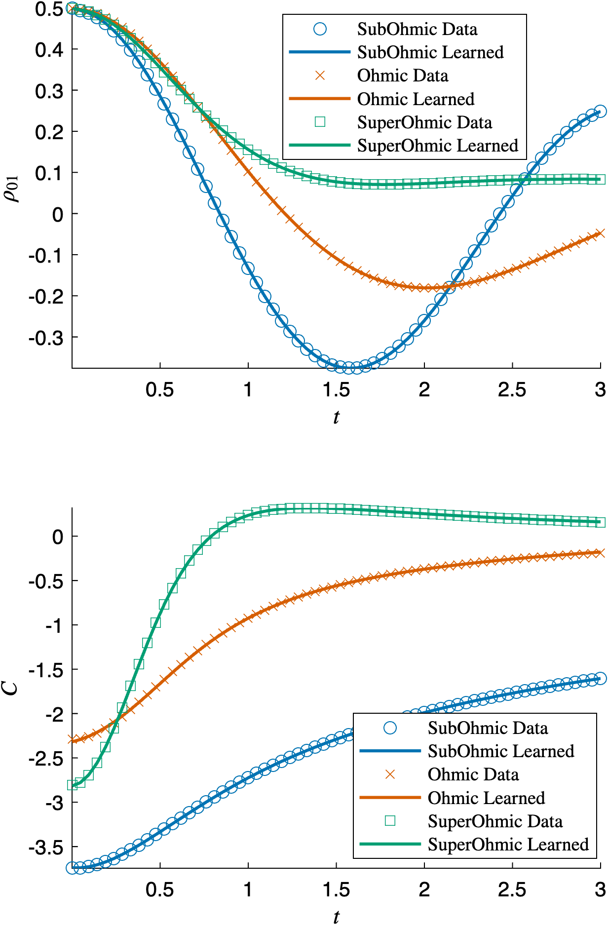
Now, we investigate the effect of corrupting our synthetic data with noise. We perturb the Ohmic data, which can be seen in the top panel of Figure 1 with a 10% relative amplitude, that is, $\rho^{w}_{01}(t)=(1+w(t))\rho^{\rm data}_{01}(t)$ where $w(t)$ is uniformly sampled on $[-1/10,1/10]$ at each time $t$. The trained dynamics, without regularization, typically yields a loss that evaluates on the order of $10^{-4}.$

Despite this somewhat small loss, we observe that the correlation function begins to exhibit a fast oscillation near $t=0.5$. To regularize this behavior, we use a homogeneous Sobolev regularization ($\beta=1$ in Equation (7)) while varying the weighting parameter $\alpha$ in eq. (8). As can be seen in Figure 2, the regularization does well to smooth out this fast oscillation, yet maintains an evaluation of the loss function that remains within the same order of magnitude as the unregularized case.

We now consider a two-level system coupled to a single quantized cavity mode under the rotating-wave approximation [43, 32], with the cavity itself leaking into a flat continuum [22]. Setting $\hbar=1$, the qubit–mode Hamiltonian is [22]

$$H=\frac{\omega_{0}}{2}\sigma_{z}+\omega_{c}\,a^{\dagger}a+g\big(\sigma_{+}a+\sigma_{-}a^{\dagger}\big),$$

(14)

where $\sigma_{\pm}$ are the qubit raising and lowering operators, $a,a^{\dagger}$ are the mode ladder operators with $[a,a^{\dagger}]=1$ (identity on the mode space), $\omega_{0}$ is the qubit splitting, $\omega_{c}$ the mode frequency, and $g$ the dipole coupling.

The cavity is lossy, and this amounts to a mode damping at linewidth $\kappa$ by a Lindblad dissipator, so the joint qubit–mode state $\chi$, a density operator on $\mathbb{C}^{2}\otimes\mathcal{F}$ with $\mathcal{F}$ the mode Fock space, obeys

	$\displaystyle\dot{\chi}$	$\displaystyle=-i[H,\chi]+\kappa\,\mathcal{D}[a]\chi,$		(15)
	$\displaystyle\mathcal{D}[a]\chi$	$\displaystyle=a\chi a^{\dagger}-\tfrac{1}{2}\big\{a^{\dagger}a,\chi\big\},$

where $\{X,Y\}=XY+YX$ denotes the anticommutator. The qubit is recovered by tracing the mode out of the joint state, $\rho(t)=\mathrm{Tr}_{\mathcal{F}}\,\chi(t)=\sum_{n}\langle n|\chi(t)|n\rangle$, the partial trace over the Fock basis $\{|n\rangle\}$ [2].

A single Lindblad-damped mode reproduces the exact reduced dynamics of a qubit coupled to a continuum reservoir of Lorentzian spectral density

$$J(\omega)=\frac{1}{2\pi}\,\frac{\gamma_{0}\kappa^{2}}{(\omega-\omega_{c})^{2}+\kappa^{2}},$$

(16)

centered at the mode frequency $\omega_{c}$, with $\gamma_{0}$ the Markovian-limit decay rate of the qubit and the cavity linewidth $\kappa$ setting the reservoir width. This is an example of what is referred to as the pseudomode correspondence in the literature [17, 15]. The practical implication is that the Markovian damping of one discrete mode reappears as a finite-width spectral feature for the qubit, and that finite width is what renders the reduced dynamics non-Markovian.

Precisely, the reservoir correlation function is the single exponential

$$f(\tau)=\frac{\gamma_{0}\kappa}{2}\,e^{-(\kappa-i\delta)\tau},\qquad\delta=\omega_{0}-\omega_{c}.$$

(17)

Restricting to the single-excitation sector, with the reservoir in vacuum and at most one quantum shared between qubit and mode, the excited-state amplitude $G(t)$ obeys the convolution equation

$$\dot{G}(t)=-\int_{0}^{t}f(t-\tau)\,G(\tau)\,d\tau,\qquad G(0)=1,$$

(18)

whose exponential kernel gives the closed form

$$G(t)=e^{-at/2}\!\left[\cosh\frac{dt}{2}+\frac{a}{d}\sinh\frac{dt}{2}\right],$$

(19)

with $a=\kappa-i\delta$ and $d=\sqrt{a^{2}-2\gamma_{0}\kappa}$; the amplitude equation and its solution are standard, and we follow Ref. [2]. In the strong-coupling regime, $d$ is imaginary and the excited-state weight $|G(t)|^{2}$ revives. This is the signature of non-Markovianity in which excitation kicks back from the reservoir to the qubit.

Meanwhile, the reduced map is the amplitude-damping channel

	$\displaystyle\rho_{11}(t)$	$\displaystyle=\rho_{11}(0)\,|G(t)|^{2},$		(20)
	$\displaystyle\rho_{01}(t)$	$\displaystyle=\rho_{01}(0)\,\overline{G(t)},$
	$\displaystyle\rho_{00}(t)$	$\displaystyle=1-\rho_{11}(t),$

written in the vectorization $\mathbf{x}=[\rho_{00},\rho_{11},\rho_{01},\rho_{10}]^{\top}$, with index $0$ the ground level and $1$ the excited level. Since $|G(t)|\leq 1$ at all times, the channel is completely positive (CP) throughout, so the synthetic training data are CP by construction with no enforcement on our part.

The model conserves the total excitation number $\sigma_{+}\sigma_{-}+a^{\dagger}a$, so the reduced generator commutes with the $\sigma_{z}$ phase rotation and the kernel

$$B_{\mathrm{JC}}(\tau)=\begin{pmatrix}0&-b_{22}(\tau)&0&0\\ 0&b_{22}(\tau)&0&0\\ 0&0&b_{33}(\tau)&0\\ 0&0&0&\overline{b_{33}(\tau)}\end{pmatrix}$$

(21)

does not mix populations with coherences. Moreover, since the coherence is linear, $\rho_{01}=\rho_{01}(0)\,\overline{G}$, conjugating (18) gives a closed convolution for $\rho_{01}$. Indeed, the coherence kernel inherits the reservoir correlation as

$$b_{33}(\tau)=-\overline{f(\tau)}.$$

(22)

For our numerical experiments, we take $\gamma_{0}=3$, $\kappa=1$, $\delta=0.5$, giving quality factor $R=2\gamma_{0}/\kappa=6$, deep in the strong coupling regime, where we see (in the state response in Figure 3) $|G(t)|^{2}$ revives near $t\approx 1.75$. Initial states are drawn from the physical set by sampling

$$R=\begin{pmatrix}s_{1}&is_{2}\\ -is_{2}&1-s_{1}\end{pmatrix},\qquad s_{1},s_{2}\sim\textrm{Uniform}(0,1),$$

which is an effective projection onto the positive semi-definite cone with unit trace. This matrix state is then vectorized to the initial state vector $x_{0}\in\mathbb{C}^{4}.$ We then integrate the channel (20) on $t\in[0,5]$ with $250$ points, so the training data are CP by construction. We model $b_{33}$ by a complex $[3/3]$ Padé and $b_{22}$ by a real $[3/3]$ Padé (denominator constant unity, $21$ real parameters), minimize the regularized objective (8) over $12$ training trajectories. We found that training over multiple trajectories improves generalization by at least an order of magnitude in this matrix-valued kernel setting.

To discuss generalization, we use the empirical risk (or held-out misfit)

$$\mathcal{R}[A,B]=\mathbb{E}_{\rho(0)\sim\varrho}\mathcal{J}_{\rm loss}[A,B].$$

(23)

At $\alpha=10^{-6}$, $\beta=0.5$ the method recovers $b_{33}=-\bar{f}$ to a relative error of $1.4\times 10^{-2}$, roughly uniform across the lag window, and a held-out misfit of $1.8\times 10^{-6}$ with minimum eigenvalue $6.1\times 10^{-5}$ across a 40 state ensemble. Additionally, the regularization we used to find this result is essential. Without the penalty ($\alpha=0$), the misfit sits at a fairly large value of $1.4\times 10^{-2}$ and the minimum eigenvalue collapses to $-3.5\times 10^{5}$. We found that $\alpha>0$ together with the derivative penalty ($\beta>0$) worked best, while too large an $\alpha$ pulls $b_{33}$ off $-\bar{f}$ and grazes the cone near $-10^{-3}$, losing the CP structure. Our results are summarized concisely in Table 1.

A similar qubit-environment Hamiltonian to that of Test Problem 1 can be used to model an interaction that does involve energy exchange and leads not only to pure dephasing, but involves the evolution of qubit occupations in any basis [13, 50, 20]. The condition is that the free qubit Hamiltonian does not commute with the interaction term [46]. To fulfill this condition, we exchange the interaction in eq. (9) as follows,

$$\sigma_{z}\sum_{k}\left(f_{k}b_{k}^{\dagger}+f_{k}^{*}b_{k}\right)\rightarrow\sigma_{x}\sum_{k}\left(f_{k}b_{k}^{\dagger}+f_{k}^{*}b_{k}\right).$$

(24)

Note, that the change in the Hamiltonian is small (limited to the exchange of the Pauli matrix that governs the effect of the interaction on the qubit), but it leads to a fundamental change of the nature of the decoherence.

Thus, now both the occupations and the coherences of the qubit state affected by the interaction with the environment, and their evolution (in the interaction picture) is governed by the following equations,

	$\displaystyle\frac{d\rho_{00}}{dt}$	$\displaystyle=-\int_{0}^{t}\!\!ds\int_{0}^{\infty}\!\!d\omega\,J(\omega)\cos\big((\varepsilon_{0}{-}\omega)(t{-}s)\big.)$
		$\displaystyle\quad\times\left[\rho_{00}(s)(2n(\omega){+}1)-\rho_{11}(s)(n(\omega){+}1)\right],$		(25a)
	$\displaystyle\frac{d\rho_{01}}{dt}$	$\displaystyle=-\frac{1}{2}\int_{0}^{t}\!\!ds\int_{0}^{\infty}\!\!d\omega\,J(\omega)(2n(\omega){+}1)$
		$\displaystyle\quad\times\big[\,\rho_{01}(s)e^{-i(\varepsilon_{0}{-}\omega)(t{-}s)}$
		$\displaystyle\qquad\quad-\rho_{10}(s)e^{-2i\varepsilon_{0}t}e^{i(\varepsilon_{0}{-}\omega)(t{-}s)}\,\big],$		(25b)

together with the closure relations $\rho_{00}(t)+\rho_{11}(t)=1$ and $\rho_{10}(t)=\rho_{01}^{*}(t)$. Here, it was assumed that the initial state of the environment is a thermal equilibrium state with respect to its free Hamiltonian.

The population equations are already convolutions in the lag $t-s$, but the $\rho_{10}$ term in eq. (25) carries an explicit factor $e^{-2i\varepsilon_{0}t}$ that depends on absolute time, so the coherence block is two-time and eq. (25) is not yet of the convolution form (3). We remove this factor by passing to the co-rotating coherence variables

$$\tilde{\rho}_{01}(t)=e^{i\varepsilon_{0}t}\rho_{01}(t),\qquad\tilde{\rho}_{10}(t)=e^{-i\varepsilon_{0}t}\rho_{10}(t),$$

(26)

with the populations unchanged. The phases $e^{\pm i\varepsilon_{0}t}$ carried by $\rho_{01}$ and $\rho_{10}$ cancel the $e^{-2i\varepsilon_{0}t}$ in the cross term, and every bracket in eq. (25) reduces to a function of $t-s$ alone. In the variables $\mathbf{x}=[\rho_{00},\rho_{11},\tilde{\rho}_{01},\tilde{\rho}_{10}]^{\top}$ the dynamics are then exactly of the form (3), with the frame rotation carried by a local generator

$$A=\mathrm{diag}\!\left(0,\,0,\,i\varepsilon_{0},\,-i\varepsilon_{0}\right),$$

(27)

and a genuine convolution kernel of the block form

$$B=\left(\begin{array}[]{cccc}B_{00}&B_{11}&0&0\\ -B_{00}&-B_{11}&0&0\\ 0&0&B_{01}&B_{10}\\ 0&0&B_{10}^{*}&B_{01}^{*}\end{array}\right).$$

(28)

This convolution form, not available in the original interaction frame, is what lets us learn both $A$ and $B$ with the lag-only ansatz (4) against the optimization problem (8). We see something similar in Sec. VI, where the qubit splitting is again carried by $A$ and the kernel is a pure convolution. This desirable block matrix structure in the correlation kernel is one reason why we vectorize the density matrix in the specific way chosen in the context of eq. (3).

In the following, we use almost all of the same parameters as in Test Problem 1. Of the parameters that enter the spectral density given by eq. (13), we only change the parameter $g$ to $g=1/4$ responsible for the overall strength of the coupling, in order to be in the weak coupling limit. We also set the qubit energy splitting $\varepsilon_{0}=1$; this parameter did not affect the evolution in the previous example (while in the interaction picture), thus it was not set. Initial states are drawn from the physical set by sampling just as in Section IV.

Generating synthetic data is now more expensive than in the previous case. We must compute quadratures over the angular frequency $\omega$ to numerically access the correlation functions. Since these functions must be recomputed at every instance of time $t$, the full dynamics are costly to construct. To accurately generate the data within an absolute error of $10^{-6}$ at time $t=3$ using 32 grid points, we must use a frequency cutoff of $\Omega=1000$ and $2^{18}$ uniformly spaced frequency points for a numerical integration over $\omega$ using the trapezoidal rule.

To learn each of the four correlation functions, we found it sufficient to use a $[3/3]$ Padé approximant. Empirically for this case study, we found regularization parameters of $\alpha=10^{-4}$ and $\beta=0.95$ worked sufficiently well to dampen sharp oscillations almost surely to appear without regularization. We mention in passing that we found it difficult to find a good value of $\alpha$ when $\beta=1$, and this is the main reason why we introduce the parameter $\beta$ into the regularization given by eq. (7).

The frame rotation (26) is part of what is learned, and the optimizer recovers $A_{33}=i\varepsilon_{0}$ as $-0.07+1.01$.

We also find that the dynamics generated by our learned correlation functions do not generalize from learning a single trajectory. Instead, we train on 30 trajectories evolved from initial conditions sampled from the space $\varrho$ of density matrices, that is, initial conditions that lead to a $\rho(0)$ with unit trace and real, positive eigenvalues.

The empirical risk, given by Equation 23, evaluated over 100 out-of-training samples is $1.9\times 10^{-4}$, the same order as the training risk $1.8\times 10^{-4}$ while the minimum eigenvalue of $\rho$ over the entire ensemble remains positive. Therefore, we are left to conclude that our trained model generalizes to out of training samples and remains CP despite an inaccurate identification of the correlation function. We summarize these results visually in Figure 5 and revisit the misidentification of the kernel in Section VII.

The three preceding tests each supplied an analytic kernel to check against. The same qubit-and-damped-mode apparatus of Sec. IV, with the counter-rotating terms restored, fails to admit an exact kernel. Therefore, numerical methods for kernel identification (should one choose to model the dynamics using the Nakajima-Zwanzig route) become essential. In this section, the ground truth is numerically accessed from an exact reduction, helping to keep the construction of the test data provably physical.

The qubit and one bosonic mode live on $\mathcal{H}=\mathbb{C}^{2}\otimes\mathbb{C}^{N_{\mathrm{ph}}}$, where the mode Fock space is truncated to $N_{\mathrm{ph}}$ levels. The Hamiltonian restores the counter-rotating terms dropped in Sec. IV,

$$H=\frac{\omega_{q}}{2}\,\sigma_{z}\otimes I+\omega_{c}\,I\otimes a^{\dagger}a+g\,\sigma_{x}\otimes\big(a+a^{\dagger}\big),$$

(29)

and the joint state $\chi$ evolves under a Lindblad master equation with the mode damped at rate $\kappa$,

	$\displaystyle\dot{\chi}$	$\displaystyle=-i[H,\chi]+\kappa\,\mathcal{D}[a]\chi,$		(30)
	$\displaystyle\mathcal{D}[a]\chi$	$\displaystyle=a\chi a^{\dagger}-\tfrac{1}{2}\{a^{\dagger}a,\chi\}.$

To integrate (30) we column-stack $\chi\in\mathbb{C}^{d\times d}$, $d=2N_{\mathrm{ph}}$, into $\mathrm{vec}(\chi)\in\mathbb{C}^{d^{2}}$ and use the identity $\mathrm{vec}(M\chi M^{\prime})=(M^{\prime\top}\otimes M)\,\mathrm{vec}(\chi)$. Applied term by term to (30), the commutator becomes $-i(I\otimes H-H^{\top}\otimes I)$, the gain term $a\chi a^{\dagger}$ becomes $\bar{a}\otimes a$ (since $(a^{\dagger})^{\top}=\bar{a}$), and the two anticommutator terms become $-\tfrac{1}{2}I\otimes a^{\dagger}a$ and $-\tfrac{1}{2}(a^{\dagger}a)^{\top}\otimes I$, so the generator is the constant matrix

$$\mathcal{L}=-i\big(I\otimes H-H^{\top}\otimes I\big)+\kappa\Big(\bar{a}\otimes a-\tfrac{1}{2}I\otimes a^{\dagger}a-\tfrac{1}{2}(a^{\dagger}a)^{\top}\otimes I\Big).$$

(31)

Because $\mathcal{L}$ is time-independent, the exact one-step propagator is the matrix exponential $P=e^{\mathcal{L}h}$ on the uniform grid $t_{n}=nh$, evaluated once. A trajectory is the orbit $\mathrm{vec}(\chi_{n+1})=P\,\mathrm{vec}(\chi_{n})$ from the factorized vacuum initial condition $\chi_{0}=\rho_{0}\otimes|0\rangle\langle 0|$, is exact to machine precision at the grid points.

The reduced qubit state is recovered at each step by the partial trace over the mode. Writing $\chi_{n}$ in $2\times 2$ block form with blocks of size $N_{\mathrm{ph}}$,

$$\chi_{n}=\begin{pmatrix}\chi^{(n)}_{00}&\chi^{(n)}_{01}\\[2.0pt] \chi^{(n)}_{10}&\chi^{(n)}_{11}\end{pmatrix},\qquad(\rho_{n})_{ij}=\mathrm{Tr}\big(\chi^{(n)}_{ij}\big),$$

so each reduced matrix element is the trace of one block. The reduced (and vectorized) state data $\{\mathbf{x}_{n}\}$ is then a partial trace of a completely positive joint evolution, hence CP and trace-preserving for every coupling strength and every truncation $N_{\mathrm{ph}}$. Initial states are drawn from the physical set, once again, as in Section IV.

We now consider the finite-dimensional operators $A$ and $B$ in this setting. The instantaneous reduced generator is the projected Liouvillian $A=\mathcal{P}\mathcal{L}\mathcal{P}$, where $\mathcal{P}$ is the factorized-vacuum projector. Both the coupling and the dissipator have zero expectation in the mode vacuum, so $A$ reduces to the bare qubit rotation,

$$A=-i[H_{S},\,\cdot\,]=\mathrm{diag}\big(0,\,0,\,-i\omega_{q},\,+i\omega_{q}\big).$$

(32)

Meanwhile, the kernel inherits sparsity from the joint parity $\Pi=\sigma_{z}\otimes e^{i\pi a^{\dagger}a}$, which commutes with $H$ and leaves $\mathcal{D}[a]$ invariant, and so commutes with the Nakajima–Zwanzig kernel for any coupling strength. On the reduced qubit, $\Pi$ acts as $\rho\mapsto\sigma_{z}\rho\sigma_{z}$, and alongside trace preservation and Hermiticity, the admissible kernel is of the form

$$B_{\mathrm{Rabi}}(\tau)=\begin{pmatrix}b_{11}&b_{12}&0&0\\ -b_{11}&-b_{12}&0&0\\ 0&0&b_{33}&b_{34}\\ 0&0&\overline{b_{34}}&\overline{b_{33}}\end{pmatrix}.$$

(33)

Note that this is the same block sparsity as the transverse Born kernel of Sec. V.

Our numerical methodology requires two further ingredients to meet the challenge of this problem. First, we observed that random multi-starting for our deployed line searches stalls. The transverse coupling lands the initial residual at $\mathcal{O}(10)$ with first-order optimality $\sim 10^{4}$. To overcome this, we seed instead from transfer tensors [8] (which can also be realized through quantum process tomography in an experimental setting [10]). The reduced dynamical map $\mathcal{E}(t)$, defined by $\mathbf{x}(t)=\mathcal{E}(t)\mathbf{x}_{0}$, obeys the same Volterra equation as the state,

$$\dot{\mathcal{E}}(t)=A\,\mathcal{E}(t)+\int_{0}^{t}B(t-\tau)\,\mathcal{E}(\tau)\,d\tau,\qquad\mathcal{E}(0)=I,$$

(34)

and we obtain $\mathcal{E}_{n}$ at the grid points directly, by propagating the four basis density matrices $\{E_{11},E_{22},E_{12},E_{21}\}$ under $e^{\mathcal{L}h}$ and reading their reduced images as the columns of $\mathcal{E}_{n}$. Discretizing (34) with a backward difference for the derivative and a rectangle rule for the memory integral gives a recursion that isolates the discrete kernel at each step,

$$B_{n}=\frac{1}{h}\left(\frac{\mathcal{E}_{n}-\mathcal{E}_{n-1}}{h}-A\,\mathcal{E}_{n}-h\sum_{m=1}^{n-1}B_{n-m}\,\mathcal{E}_{m}\right),$$

(35)

where $A$ is the known local generator of Eq. (32). This amounts to a causal deconvolution that returns $B_{n}$ from the already-known $B_{1},\dots,B_{n-1}$. Then, fitting a Padé entry to this discrete kernel supplies the seed. From this seed, the Levenberg–Marquardt solver of Sec. II drops the residual by an order of magnitude within a few iterations.

Second, we found the $H^{1}$ penalty could not effectively suppress spurious behavior. We instead address this structurally by writing each denominator as a product of decaying factors,

$$\mathrm{den}(\tau)=\prod_{i}\Big(1+\tau\,e^{-\xi_{i}}\Big),$$

(36)

so every pole sits at $\tau=-e^{\xi_{i}}<0$, on the decaying side of the origin and never in $[0,T]$, for any real $\xi_{i}$. The optimizer then works over the unconstrained log-rates $\xi_{i}\in\mathbb{R}$, which both removes the constraint boundary and conditions the denominator gradient, since $\partial_{\xi_{i}}$ acts smoothly on $e^{-\xi_{i}}$.

For the numerical experiment we take $\omega_{q}=\omega_{c}=1$, $g=0.4$ (well outside the rotating-wave regime), $\kappa=0.5$, and $N_{\mathrm{ph}}=8$, on $t\in[0,12]$ with $N_{t}=120$. The four independent kernel functions $b_{11},b_{12},b_{33},b_{34}$ of Eq. (33) are modeled as factored-pole $[3/3]$ Padé functions and fit over $10$ training trajectories at $\alpha=10^{-4}$, $\beta=1$. Direct simulation confirms the data are CP (worst training minimum eigenvalue $5.2\times 10^{-3}$).

The learned model reproduces held-out trajectories to a cross-validation misfit of $6.8\times 10^{-4}$ (training $7.5\times 10^{-4}$), shown with the recovered kernel in Fig. 6. The learned kernel here grazes the boundary of the physical set. The worst-case minimum eigenvalue over $40$ held-out states is $8.2\times 10^{-4}$, positive but two orders of magnitude inside the data’s own margin of $1.0\times 10^{-1}$, whereas the Jaynes–Cummings fit stayed level with the data. We comment that the reduced-model error is known to be mostly in the fidelity of the kernel. Against the full Fock propagation at $N_{t}=4096$, the solver’s time-grid error at $N_{t}=256$ is $7.3\times 10^{-14}$ and refining $N_{\mathrm{ph}}=8\to 16$ moves the reference by $3.4\times 10^{-7}$, both far below the learned relative error $1.1\times 10^{-2}$.

In the matrix-valued cases of Secs. V and VI, the recovered kernels differ from the generating kernels while the state dynamics generalize. This property has also been observed in generalized Langevin and projection-operator models [33, 54, 9, 28, 23]. To make quantitative statements about our numerical kernel identification here, we measure the conditioning of kernel recovery in a parametrization-invariant way, and then decompose the realized kernel error in its sensitivity basis. This helps provide a standardized account of a kernel with an error of order one, responsible for a relative state error of order $10^{-2}$.

To begin, we write the kernel through its parameters $\theta\in\mathbb{R}^{N_{\xi}}$ and stack the model output, the density-matrix trajectories over a fixed ensemble of $K$ initial states, into one vector $\mathbf{F}(\theta)\in\mathbb{R}^{P}$, $P=2dN_{t}K$. The local difficulty of recovering $\theta$ is set by the Jacobian, computed via

$$G_{im}=\frac{\partial F_{i}}{\partial\theta_{m}},\qquad G\in\mathbb{R}^{P\times N_{\xi}},$$

(37)

and formed by forward differences with step $10^{-6}$. To see this, use the singular value decomposition (SVD) $G=U\Sigma V^{\top}$, and consider a kernel perturbation $\delta\theta=\sum_{m}c_{m}\mathbf{v}_{m}$ (in the right singular basis spanned by $\{v_{m}\}$). The perturbation moves the trajectories by

$$\|G\,\delta\theta\|_{\ell^{2}(\mathbb{R}^{P})}^{2}=\sum_{m}\sigma_{m}^{2}\,c_{m}^{2}.$$

(38)

Meanwhile, a data error $\delta\mathbf{d}$ produces the reconstruction error via the pseudoinverse written in the SVD basis

$$\delta\theta=\sum_{m}\frac{\mathbf{u}_{m}^{\top}\delta\mathbf{d}}{\sigma_{m}}\,\mathbf{v}_{m},$$

(39)

We see that Eq. (38) scales the data error by $\sigma_{m}$ while Eq. (39) scales the recovered kernel error by $1/\sigma_{m}$ for a data error in the same direction. Therefore, a small $\sigma_{m}$ means a weakly constrained kernel and a weakly informative data direction.

However, the raw spectrum of $G$ is not intrinsic, since $\sigma_{m}$ measures sensitivity per unit change of parameters, which in principle induces an arbitrary coordinate system on kernel space. Under a smooth reparametrization $\theta=\phi(\eta)$ with coordinate Jacobian $C=\partial\theta/\partial\eta$, both Jacobians transform as $G\mapsto GC$ and $J\mapsto JC$, so the singular values of $G$ mix the physics of the inverse problem with the conditioning of the Padé coordinates. To remove the coordinate dependence we measure sensitivity per unit change of the function $B$.

To this end, let $\mathbf{b}(\theta)$ be the four kernel functions sampled on the lag grid, with real and imaginary parts stacked into $8N_{t}$ entries. Write its Jacobian $J_{im}=\partial b_{i}/\partial\theta_{m}$ and let $W=\mathrm{diag}(\mathbf{w})$ hold the trapezoidal quadrature weights, so that $\mathbf{b}^{\top}W\,\mathbf{b}\approx\|B\|_{L^{2}}^{2}$. The parametrization-invariant sensitivities are then simply determined by the stationary values of the ratio $\|G\,\delta\theta\|_{2}^{2}/\|J\,\delta\theta\|_{W}^{2}$, interpreted as the data response per unit $L^{2}$ change of the kernel, whose Euler equation is the generalized eigenproblem [18]

$$G^{\top}G\,\mathbf{v}_{m}=\lambda_{m}\,(J^{\top}WJ)\,\mathbf{v}_{m}.$$

(40)

The sensitivities are $\sigma_{m}^{\mathrm{inv}}=\sqrt{\lambda_{m}}$ and it’s easy to see that they are the data change per unit change in $\|B\|_{L^{2}}$ along $\mathbf{v}_{m}$. Indeed, under a reparametrization $\theta=\phi(\eta)$ with $C=\partial\theta/\partial\eta$, Eq. (40) transforms to

$$C^{\top}G^{\top}G\,C\,\mathbf{w}_{m}=\lambda_{m}\,C^{\top}J^{\top}WJ\,C\,\mathbf{w}_{m}.$$

(41)

The factor $C^{\top}(\cdot)\,C$ common to both sides cancels, so the $\lambda_{m}$, and hence $\sigma_{m}^{\mathrm{inv}}$, are unchanged by the reparametrization. Each $\sigma_{m}^{\mathrm{inv}}$ gives the change in the data per unit change in $\|B\|_{L^{2}}$, as desired. See  [39] for further detail.

To evaluate spectra for the transverse Born model, we solve Eq. (40) as a dense generalized eigenproblem. We do so on the two available kernels, the learned and the true, in the gauge-fixed $[3/3]$ Padé class, with the denominator constant divided out to remove the rational scale redundancy. We find that the coordinate spectrum $\sigma_{m}$ spans about seven orders of magnitude, while the invariant spectra $\sigma_{m}^{\mathrm{inv}}$ (shown in Fig. 7) span about three, showing the merit of using the coordinate invariant approach to isolate the native function space ill-conditioning of the inverse problem.

Let $\theta^{\mathrm{true}}$ and $\theta^{*}$ respectively denote the true and identified kernels projected onto the same gauge-fixed $[3/3]$ class, and form $\delta\theta=\theta^{\ast}-\theta^{\mathrm{true}}$. We find that $\|\delta\theta\|_{2}=2.24$, an order-one discrepancy consistent with the entrywise mismatch of Fig. 5. We build $G$ at $\theta^{\mathrm{true}}$ and take its SVD $G=U\Sigma V^{\top}$ with $\sigma_{1}\geq\cdots\geq\sigma_{N_{\xi}}$, and expand $\delta\theta=\sum_{m}c_{m}\mathbf{v}_{m}$ with $c_{m}=\mathbf{v}_{m}^{\top}\delta\theta$. The fraction of the error captured by the first $m$ directions is

$$E(m)=\frac{\sum_{k\leq m}c_{k}^{2}}{\sum_{k}c_{k}^{2}},$$

(42)

and, since direction $k$ moves the data by $\sigma_{k}c_{k}$ from (38), the fraction of the data response carried by the first $m$ directions is

$$D(m)=\frac{\sum_{k\leq m}\sigma_{k}^{2}c_{k}^{2}}{\sum_{k}\sigma_{k}^{2}c_{k}^{2}}.$$

(43)

Ordered by decreasing data sensitivity (Fig. 8), we find that the top two directions carry $90\%$ of the data response and the top thirteen carry $99\%$, while those same two hold $0.2\%$ of the kernel error and the top thirteen hold $0.6\%$. Thresholding by conditioning instead of by count, the directions with $\sigma_{m}<10^{-2}\sigma_{1}$ hold $96.2\%$ of the kernel error and contribute $0.3\%$ of the data response. Thus, the error and the data response occupy nearly disjoint subspaces.

We proposed a direct, data driven route to non Markovian dynamics by learning the Volterra kernel in the Nakajima Zwanzig representation. The guiding principle was to keep the hypothesis class minimal: each scalar component of the kernel is modeled by a fixed-order Padé rational function in the lag variable, and the search is regularized by an $H^{1}$ penalty. In the scalar setting the learning problem is straightforward and we find that fits are stable, trajectories are accurate, and the optimization landscape behaves predictably. Difficulties appear once we are in the matrix-valued kernel case, and require the introduction of two more ingredients, namely, transfer tensor seeding and a factored pole form of the Padé ansatz. Furthermore, non identifiability issues arise, and the behavior can no longer be attributed to the Padé model itself but rather to the structure induced by the operator-valued coupling. This point was elucidated in Section VII.

Within this simple framework, a simple nonlocal Crank Nicolson discretization recovers accurate state trajectories across four increasingly challenging test beds: pure dephasing, a damped Jaynes–Cummings model with an analytic coherence kernel, a transverse Born model with decoherence and population decay, and a non-rotating-wave quantum Rabi model which lacks a closed-form memory kernel. On the analysis side, we established regularity for $B\in H^{1}$ and existence of minimizers for the regularized problem, which gives a basic well posedness foundation for learning operator-valued kernels.

The approach has clear limitations. First, identifiability of $(A,B)$ from finite time windows and finite state sampling is delicate. Distinct operator-valued kernels can generate nearly indistinguishable trajectories on $[0,T]$, and our results show that accurate state fits do not guarantee pointwise kernel recovery, a mechanism we quantify in Sec. VII. Second, we did not enforce complete positivity. Trace preservation and Hermiticity are respected by construction, but CP is only implicit and may fail outside the training window. Third, Padé models can introduce spurious poles and local oscillations near the origin in noisy settings. The $H^{1}$ penalty mitigates this behavior, and the factored-pole parametrization (36) removes it structurally by placing every denominator root off the lag window, yet, as can be seen in Figure 6, sharp features in kernel recovery may still remain. Beyond larger systems, another extension is to driven qubits, where $H_{S}(t)$ genuinely makes the kernel two-time. The lag-only rational ansatz no longer applies, yet a separable representation in the two time arguments is the natural replacement. Finally, the nonlocal stepping with a dense history is computationally heavy, with quadratic scaling in $N_{t}$, which limits long horizon training and broad hyperparameter sweeps.

References

- [1] (2004) Barycentric lagrange interpolation. SIAM Rev. 46 (3), pp. 501–517. Cited by: Appendix B, §VIII.
- [2] (2002) The theory of open quantum systems. Oxford University Press. Cited by: §I, §II, §II, §II, §II, §III, §IV, §IV, §VIII.
- [3] (2006-01) Non-markovian quantum dynamics: correlated projection superoperators and hilbert space averaging. Phys. Rev. E 73, pp. 016139. Cited by: §II.
- [4] (1999-02) Stochastic wave-function method for non-markovian quantum master equations. Phys. Rev. A 59, pp. 1633–1643. Cited by: §II.
- [5] (2001) The time-convolutionless projection operator technique in the quantum theory of dissipation and decoherence. Annals of Physics 291 (1), pp. 36–70. External Links: ISSN 0003-4916 Cited by: §II.
- [6] (2010) Functional analysis, sobolev spaces and partial differential equations. Springer. Cited by: Appendix C.
- [7] (2014-12) Identifying a bath-induced bose liquid in interacting spin-boson models. Phys. Rev. Lett. 113, pp. 260403. Cited by: §III.
- [8] (2014) Non-markovian dynamical maps: numerical processing of open quantum trajectories. Phys. Rev. Lett. 112, pp. 110401. Cited by: §I, §II, §VI.
- [9] (2013) Stochastic tools in mathematics and science. 3rd edition, Springer. Cited by: §I, §VII.
- [10] (1997) Prescription for experimental determination of the dynamics of a quantum black box. Journal of Modern Optics 44 (11–12), pp. 2455–2467. Cited by: §VI.
- [11] (2012) Quantification of memory effects in the spin-boson model. Phys. Rev. A 86, pp. 012115. Cited by: §I.
- [12] (2017) Dynamics of non-markovian open quantum systems. Rev. Mod. Phys. 89, pp. 015001. Cited by: §I, §II, §II, §VIII.
- [13] (2005-01) Rigorous born approximation and beyond for the spin-boson model. Phys. Rev. B 71, pp. 035318. Cited by: §V.
- [14] (2010) Partial differential equations. 2 edition, American Mathematical Society. Cited by: Appendix C.
- [15] (2017-02) Exact non-markovian master equation for the spin-boson and jaynes-cummings models. Phys. Rev. A 95, pp. 020101. Cited by: §III, §IV.
- [16] (2005-02) Full counting statistics of nano-electromechanical systems. Europhysics Letters 69 (3), pp. 475–481. Cited by: §I.
- [17] (1997-03) Nonperturbative decay of an atomic system in a cavity. Phys. Rev. A 55, pp. 2290–2303. Cited by: §I, §IV.
- [18] (2013) Matrix computations. 4th edition, Johns Hopkins University Press, Baltimore. Cited by: §VII.
- [19] (1976) Completely positive dynamical semigroups of n‐level systems. Journal of Mathematical Physics 17 (5), pp. 821–825. Cited by: §II, §VIII.
- [20] (2023-05) Signatures of non-markovianity of a superconducting qubit. Phys. Rev. B 107, pp. 174511. Cited by: §V.
- [21] (2012-04) Critical and strong-coupling phases in one- and two-bath spin-boson models. Phys. Rev. Lett. 108, pp. 160401. Cited by: §III.
- [22] (1963) Comparison of quantum and semiclassical radiation theories with application to the beam maser. Proc. IEEE 51 (1), pp. 89–109. Cited by: §I, §IV.
- [23] (2017) Iterative reconstruction of memory kernels. J. Chem. Theory Comput. 13 (6), pp. 2481–2488. Cited by: §I, §VII.
- [24] (2020) Unboxing quantum black box models: learning non-markovian dynamics. arXiv preprint arXiv:2009.03902. Cited by: §I.
- [25] (2002) Theory of pure dephasing and the resulting absorption line shape in semiconductor quantum dots. Phys. Rev. B 65, pp. 195313. Cited by: §I.
- [26] (2017-07) Objectivity in the non-markovian spin-boson model. Phys. Rev. A 96, pp. 012120. Cited by: §II, §III.
- [27] (1987-01) Dynamics of the dissipative two-state system. Reviews of Modern Physics 59 (1), pp. 1–85. Cited by: §I, §II, §III.
- [28] (2017) Computing the non-markovian coarse-grained interactions derived from the mori–zwanzig formalism in molecular systems: application to polymer melts. J. Chem. Phys. 146, pp. 014104. Cited by: §I, §VII.
- [29] (1976) On the generators of quantum dynamical semigroups. Communications in Mathematical Physics 48 (2), pp. 119–130. Cited by: §II, §VIII.
- [30] (1999) System identification: theory for the user. 2nd edition, Prentice Hall, Upper Saddle River, NJ. Cited by: §VIII.
- [31] (1988) Convolution quadrature and discretized operational calculus. i. Numer. Math. 52, pp. 129–145. Cited by: Appendix B, §VIII.
- [32] (2007) Elements of quantum optics. 4 edition, Springer, Berlin, Heidelberg. External Links: ISBN 978-3-540-74209-8 Cited by: §IV.
- [33] (1965) Transport, collective motion, and brownian motion. Prog. Theor. Phys. 33, pp. 423–455. Cited by: §I, §VII.
- [34] (1958) On quantum theory of transport phenomena. Prog. Theor. Phys. 20, pp. 948–959. Cited by: §I, §II, §II.
- [35] (2018) The aaa algorithm for rational approximation. SIAM J. Sci. Comput. 40 (3), pp. A1494–A1522. Cited by: Appendix B, §VIII.
- [36] (2020) Machine learning for molecular simulation. Annu. Rev. Phys. Chem. 71, pp. 361–390. Cited by: §I.
- [37] (2018) Operational markov condition for quantum processes. Phys. Rev. Lett. 120, pp. 040405. Cited by: §I.
- [38] (2010) Phonon-induced rabi-frequency renormalization of optically driven single ingaas/gaas quantum dots. Phys. Rev. Lett. 104, pp. 017402. Cited by: §I.
- [39] (1945) Information and the accuracy attainable in the estimation of statistical parameters. Bulletin of the Calcutta Mathematical Society 37, pp. 81–91. Cited by: §VII.
- [40] (2012) Open quantum systems: an introduction. Springer. Cited by: §I, §II, §II, §VIII.
- [41] (2015-09) Characterization and measurement of qubit-environment-entanglement generation during pure dephasing. Phys. Rev. A 92, pp. 032310. Cited by: §III.
- [42] (2018-11) Criteria for system-environment entanglement generation for systems of any size in pure-dephasing evolutions. Phys. Rev. A 98, pp. 052344. Cited by: §III.
- [43] (1997) Quantum optics. Cambridge University Press, Cambridge. Cited by: §IV.
- [44] (2026-07) Learning thermodynamic master equations for open quantum systems. Quantum 10, pp. 2151. External Links: ISSN 2521-327X, 2506.01882 Cited by: §I.
- [45] (1977) A generalized stochastic liouville equation. non-markovian versus memoryless master equations. Journal of Statistical Physics 17 (2), pp. 171–187. Cited by: §II, §II.
- [46] (2024-03) Qubit-environment entanglement in time-dependent pure dephasing. Phys. Rev. A 109, pp. 032412. Cited by: §V.
- [47] (2011-09) Markovianity and non-markovianity in quantum and classical systems. New Journal of Physics 13 (9), pp. 093004. Cited by: §VIII.
- [48] (2019-05) Machine learning of coarse-grained molecular dynamics force fields. ACS Central Science 5 (5), pp. 755–767. Cited by: §I.
- [49] (1999) Quantum dissipative systems. 2nd edition, World Scientific. Cited by: §I, §II.
- [50] (2017-09) Effects of counter-rotating-wave terms on the non-markovianity in quantum open systems. Phys. Rev. A 96, pp. 032125. Cited by: §V.
- [51] (1985) Nonlinear functional analysis and its applications. Springer, New York. External Links: ISBN 978-0-387-90915-8 Cited by: Appendix C.
- [52] (2003-05) Decoherence, einselection, and the quantum origins of the classical. Rev. Mod. Phys. 75, pp. 715–775. Cited by: §III.
- [53] (1960) Ensemble method in the theory of irreversibility. J. Chem. Phys. 33, pp. 1338. Cited by: §I, §II, §II.
- [54] (2001) Nonequilibrium statistical mechanics. Oxford University Press. Cited by: §I, §VII.