A whole-brain model of amyloid beta accumulation and cerebral hypoperfusion in Alzheimer’s disease
Abstract
Accumulation of amyloid beta proteins is a defining feature of Alzheimer’s disease, and is usually accompanied by cerebrovascular pathology. Evidence suggests that amyloid beta and cerebrovascular pathology are mutually reinforcing; in particular, amyloid beta suppresses perfusion by constricting capillaries, and hypoperfusion promotes the production of amyloid beta. Here, we propose a whole-brain model coupling amyloid beta and blood vessel through a hybrid model consisting of a reaction–diffusion system for the protein dynamics and porous–medium model of blood flow within and between vascular networks: arterial, capillary and venous. We discretize the resulting parabolic–elliptic system of PDEs by means of a high-order discontinuous Galerkin method in space and an implicit Euler scheme in time. Simulations in realistic brain geometries demonstrate the emergence of multistability, implying that a sufficiently large pathogenic protein seeds is necessary to trigger disease outbreak. Motivated by the ‘two-hit vascular hypothesis’ of Alzheimer’s disease that hypoperfusive vascular damage triggers amyloid beta pathology, we also demonstrate that localized hypoperfusion, in response to injury, can destabilize the healthy steady state and trigger brain-wide disease outbreak.
1 Introduction

Alzheimer’s disease (AD) is a progressive neurodegenerative disorder characterized by neuronal loss and impaired synaptic communication. It has long been established that the spread of misfolded, prion-like proteins plays a central role in AD and related disorders [57]. In particular, disease onset is associated with the accumulation of two pathological proteins: amyloid-beta (Aβ) and tau [24]. Cerebrovascular abnormalities frequently accompany AD pathology—for instance, cerebral amyloid angiopathy occurs in more than of AD cases [28], and reductions in cerebral blood flow (CBF) represent one of the earliest measurable biomarkers of the disease [30].
The interplay between Aβ and cerebral blood flow is well documented. Aβ acts as a vasoconstrictor, increasing vascular resistance and thereby reducing CBF [64, 47]. Oligomeric Aβ induces the release of vasoconstrictive agents such as endothelin-1 and generates oxidative stress, which can result in capillary occlusion [17, 48]. Conversely, hypoxia accelerates amyloid precursor protein (APP) processing and impairs its clearance across the blood–brain barrier, promoting Aβ accumulation [38, 62]. Hypoperfusion-induced injury can further exacerbate APP aggregation, possibly as a compensatory mechanism [59, 27]. Collectively, these mechanisms give rise to a positive feedback loop between Aβ buildup and vascular dysfunction [29, 34, 38]. Several studies even suggest that vascular damage may act as an early trigger for Aβ pathology in AD [72, 37].
Mathematical models.
In recent years, several mathematical models for the dynamics of prion-like proteins have been proposed. The description of the phenomena requires models based on partial differential equations (PDEs) able to describe both the temporal and the spatial dynamics of the phenomena, typically at organ scale. One example developed to describe the dynamics of Aβ is the Smoluchowski-type models [8, 22], which are derived from microscopical interactions and distinguishes different sizes of pathological aggregates [23]. Some simplified models focus on the interactions between healthy and misfolded proteins, such as the heterodimer model [21, 46], or only on the misfolded proteins population, such as the Fisher-Kolmogorov equation [69]. These simplified yet informative models offer the key advantage that they can be fully validated against existing data, while also accurately predicting disease progression at both the personalized and regional scales [11]. Furthermore, the much smaller number of physical parameters relative to Smoluchowski-type models makes the calibration procedure significantly more tractable [13, 16]. They have also been extended to describe connections with other physical phenomena occurring in AD. For example, the elastic deformations due to atrophy [56, 70, 50], the clearance mechanisms [9], the interactions with tau proteins [65], and brain activity [26, 3].
However, little attention has been devoted to the development of models coupling Aβ and CBF. In [1], the authors propose a modification of the heterodimer model on networks which takes into account CBF reduction. The first goal of the current work is to build on this idea by developing a continuous PDE model of Aβ accumulation in the brain describing also the interactions with the cerebral microvasculature through (a) vasoconstriction and (b) perfusion-dependent Aβ production and clearance (see Figure 1). Our model is based on the heterodimer model for the Aβ-dynamics description and on a multiple-network porous-medium model for the blood perfusion.
Porous-medium models have been extensively used in the context of brain poromechanics to study strokes [32, 33, 31]. Moreover, a poroelastic version of those models have been proposed to study the brain hemodynamics on the heartbeat scale [12, 40, 52, 67], and clearance mechanisms [42, 68].
In our model, we analyze the impact of Aβ on the blood flow in the capillaries, altering transfer between compartments and capillaries permeability.
Numerical methods and patient-specific simulations.
The potential clinical utility of the constructed mathematical models strongly depend on the design quality of numerical methods to simulate PDEs in patient-specific geometries. In the context of proteinopathies, connectome graph-based simulations for the models introduced in the previous section have been fully implemented [1, 9, 13, 21, 65]. However, the construction of a graph-based model for our purposes would suffer from the limitation of describing the brain’s microvasculature as a collection of small independent capillary networks, losing the coupling with the complete vasculature structure at the organ level [1].
To study physical effects in the brain, multiple works have introduced numerical discretizations of PDEs in brain geometries based on continuous finite elements [10, 40, 52, 68] and discontinuous Galerkin (dG) methods [4, 15, 12, 14, 50]. The advantage of using these high-fidelity discretizations is the possibility of constructing patient-specific computational grids from medical images and taking into account geometrical and functional information in the PDE model.
For our mathematical model, we propose a discretization based on a discontinuous Galerkin method in space and implicit Euler time stepping in time. The dG methods provide numerous advantages in our context because they are designed for high-order approximations that are of primary importance for the heterodimer system, which typically admits travelling-wave solutions [36, 4, 16]. Indeed, high-order dG schemes exhibit favourable properties for wave-like problems, allowing one to capture travelling fronts with reduced numerical dispersion and dissipation errors compared with standard low-order continuous finite element approximations as discussed in [6, 7]. Moreover, as a possible extension of the present discretization, the dG framework naturally allows for a local adjustment of the polynomial degree , which can be exploited to maintain a low computational cost through -adaptivity [41]. Additionally, they allow the use of polygonal mesh elements which is particularly useful to reduce computational costs in brain applications. Indeed, using mesh agglomeration strategies [5], the complex boundary and internal interfaces can be accurately described with a low number of mesh elements. Concerning the time discretization, the implicit Euler method is combined with a loosely-coupled strategy to solve the parabolic (heterodimer model) and elliptic (multiple-network porous-medium model) parts of the system separately.
In this work, we first carry out simulations in simplified geometries to study and understand the fundamental properties of our mathematical model. Then we perform realistic numerical simulations in brain geometries. In particular, we show the existence of multiple stable states starting from different levels of initial seeding of Aβ. Finally, we evaluate the injury-induced initiation of AD pathology, by imposing different levels of initial hypoperfusion in the frontal lobe.
Structure of the manuscript.
Section 2 is dedicated to the mathematical development of our model. We start from the presentation of the heterodimer model for Aβ spreading in Section 2.1 and the multiple-network porous-medium model in Section 2.2. Then, in Section 2.3, we propose a novel coupled mathematical model to describe the connections between Aβ and CBF. In Section 3 we introduce the discretization of the problem based on a dG-space discretization and implicit Euler time stepping. In Section 4, we present numerical simulations in simple geometries to validate the numerical solver and analyze properties of the mathematical model. In Section 5, we simulate the system in realistic three-dimensional brain geometries to study both the multistability of the system depending on the magnitude of the initial seeding and the hypoperfusion-induced pathology. Finally, in Section 6, we conclude and discuss further developments.
2 Mathematical model
2.1 Heterodimer model
We adapt Prusiner’s heterodimer prion model [53] for the protein kinetics of Aβ. That is, we assume that Aβ monomers can be either normal or pathogenic, with concentrations and , respectively. Pathogenic monomers can bind to normal monomers to form a pathogenic–normal heterodimer, which then dissociates into two pathogenic monomers. We assume that the dissociation step is fast and treat this conversion process as a single second-order chemical reaction, with rate . Normal proteins are produced at rate and cleared at rate , and pathogenic proteins are cleared at rate .
The resulting reaction–diffusion system with zero-flux boundary conditions is given by:
| (1) |
where is the diffusion tensor, is the spatial domain (i.e. the brain), is a boundary normal, and , are the initial protein concentrations. The model thus comprises an initial–boundary value problem for a parabolic system of two PDEs coupled by a nonlinear term.
The spatial transport of Aβ proteins is a combination of diffusion in the extracellular space and axonal transport. Following [70, 69], we model this combination as anisotropic diffusion whose principal direction is aligned with the brain’s axon fibers:
| (2) |
The vector field of fiber directions, , is obtained as the principal eigenvector of the diffusion tensor computed from diffusion-weighted MRI (see [15, 44]). The construction of and choice of diffusion constants is discussed in Section 5.
If the kinetic rate constants are all assumed constant, then there are two spatially-homogeneous equilibria, namely:
| healthy: | (3) | |||||||
| pathogenic: |
Crucially, the pathogenic equilibrium is positive, and therefore physically relevant, if and only if the dimensionless basic reproduction number is greater than unity. Indeed, as increases through unity, a transcritical bifurcation occurs: when , the healthy equilibrium is stable, and no other (physical) equilibrium exists, and when , the healthy equilibrium is unstable and the pathogenic equilibrium is stable (see, e.g., [1] for more details). The kinetic parameters of the heterodimer formulation can be calibrated by matching model outputs to longitudinal biomarker data and established disease time scales. Such calibration can be performed either using PET measurements, as in [11, 13] or based on employing protein concentrations derived ex vivo, as proposed in [16].
2.2 Multiple-network porous media model
For the perfusion model, our starting point is the multiple-network porous medium model proposed in [12], which is in turn inspired by [32, 31, 67].
We suppose there are three vascular networks, namely arterial, capillary, and venous, with corresponding pressure fields , , . Because the protein concentrations , evolve on timescales of hours to days, whereas , , adjust to permeability changes (e.g. due to vasoconstriction) within seconds, we assume that all pressures are quasi-static. Conservation of mass then yields the following elliptic system:
| (4) |
where and are the arterial-to-capillary and capillary-to-venous transfer coefficients. Since the brain’s capillary network is isotropic, we have assumed , and we will specify the arterial and venous permeability tensors and on a case-by-case basis in Sections 4 and 5.
Arteries spanning the pial surface of the cortex supply the brain with blood; similarly, blood is drained by the pial venous network. Accordingly, we prescribe Dirichlet boundary conditions for the arterial and venous blood pressures on the pial surface , together with a zero-flux condition for the capillary compartment:
| (5) |
The remaining part of the boundary is the brain’s ventricular surface, , where we prescribe zero-flux conditions:
| (6) |
For the perfusion model, physiologically admissible ranges for the permeability and hemodynamic parameters can be informed by recent porous-medium perfusion studies, where these quantities are inferred directly from ASL and structural MRI data [32, 33].
2.3 Coupled Aβ and perfusion model
In order to model the interaction between Aβ and the brain’s microvasculature, we couple the protein and perfusion models of Sections 2.1 and 2.2, respectively. The biological mechanisms modeled here are reviewed in [38].
First, Aβ is vasoconstrictive, i.e. it induces blood vessels to become narrow [64, 47], thus increasing vascular resistance. In particular, Nortley et al. recently found that Aβ oligomers cause brain capillaries to constrict within seconds, through a mechanism involving oxidative stress and the vasoconstrictor endothelin 1 [48]. Therefore, we assume that the permeability of the capillary bed, , is a decreasing sigmoidal function of the pathogenic protein concentration :
| (7) |
where is the base permeability (in the absence of pathogenic proteins), is the permeability for very large , and modulates the sensitivity to . At the same time, we adopt a similar strategy for the transfer coefficients and . In particular, for a generic couple , we define:
| (8) |
where is a constant that modulates the impact of misfolded Aβ on the flow between compartments. Indeed, according to the multiple-network porous medium theory developed in [2] for geophysical applications and later adapted for brain circulation in [67], the parameter models fluid exchange between networks. As discussed in [51], must be proportional to the exchange area between compartments. In Alzheimer’s disease, Aβ induces capillary constriction [48], thus reducing capillary lumen and thus decreasing and . Through these couplings, pathogenic Aβ causes local decreases in permeability (i.e. increases in resistance), which we expect to cause hypoperfusion (reduced blood flow). Finally, the choice of a sigmoidal function for the coupling is motivated by the experimental data ([48, Fig. 2D]) that shows that soluble Aβ oligomers induce a pericyte-mediated capillary constriction with a nonlinear, saturating dependence on their concentration.
Conversely, hypoperfusion increases the production rate of Aβ [59, 62, 71]; it may also decrease its clearance rate [38], though this is less certain. Therefore, we let the rates of Aβ production and clearance depend on the rate of blood flow, as follows. We define the “CBF rate” at a point as the rate of flow from the arterial compartment into the capillary bed per unit mass of tissue:
| (9) |
where is the brain tissue density estimated [33]. In the framework of the multiple-network porous-medium model, this quantity coincides with the arteriole-to-capillary exchange flux per unit tissue mass, representing the effective delivery of blood to the microvascular bed at the tissue scale. Hence, is a local proxy for CBF. Its spatial distribution and magnitude are determined by the pressure drop between arterial and capillary compartments and by the coupling coefficient , which is typically chosen in literature to be consistent with perfusion values inferred from arterial spin labelling images [32]. We denote by the healthy CBF rate, i.e. corresponding to the pressure fields , when pathogenic proteins are absent (so that there is no vasoconstriction). We now assume that the Aβ production rate increases in response to hypoperfusion, which we define as the relative decrease in from its healthy rate :
| (10) |
where is the base rate, and is the sensitivity to hypoperfusion. Similarly, we assume the clearance rates decrease in response to hypoperfusion:
| (11) |
The coupled protein–perfusion model is a parabolic–elliptic initial–boundary value problem to be solved for the concentrations , and the pressures , , :
| (12) |
The system is complemented with the following boundary conditions:
| (13) |
and with the initial conditions
| (14) |
Nondimensionalisation
For the heterodimer model, we rescale the variables as follows, where tildes indicate the new dimensionless variables [1]:
Moreover, we scale the pressure fields so as to map the interval uniformly onto :
Rescaling the equations of the system (12), we obtain the dimensionless system:
| (15) |
where
The system is complemented with the following boundary conditions:
| (16) |
and the initial data and in Equation (14) have been suitably rescaled and nondimensionalized.
Remark 2.1.
In (15), the parameter represents the ratio between the characteristic clearance time of the pathogenic species and that of the healthy one. In line with the analysis of the heterodimer–vascular model in [1], we typically have and does not act as a small parameter. This choice reflects biologically informed estimates of the underlying kinetic rates (see also the sensitivity analysis in [16]). Consequently, we do not expect a strong separation of time scales between healthy and pathogenic protein dynamics (which would lead to singular perturbation limit), and the stability analysis reported in this work arises from the nonlinear coupling mechanisms.
3 Discrete formulation
In this section, we introduce the discretization scheme for the resolution of the system in equation (12). In particular, in Section 3.1, we discuss the discretization in space, by means of a dG (discontinuous Galerkin) method, and in Section 3.2, we discretize in time by means of an implicit Euler time stepping algorithm.
3.1 Space discretization: discontinuous Galerkin method
We first introduce a mesh partition of the domain made of shape-regular simplicial elements , with corresponding diameter and define . If two elements share a common face (e.g., the triangular interface of two tetrahedra), we call it an interior face, . Otherwise, we call a boundary face, . The set is partitioned on the pial and ventricular regions of , i.e. . We now introduce the so-called trace operators. Let be a face shared by two elements . We denote by the unit normal vector to pointing outward to , respectively. Then, for sufficiently regular scalar-valued and vector-valued functions , respectively, we define the average operator as , and , and the jump operator as , and . The superscripts denote the traces on the face of the functions defined on . Analogously, on the face of a cell , we define the average operator as and , and the jump operator as and , where and are regular enough Dirichlet boundary data and is the outward unit normal vector to .
Let us define as the space of polynomials of total degree over a mesh element . Then we can introduce the following definitions of dG finite element spaces . From now on, we introduce also a shorthand notation for the integrals over the faces , and the notation to denote the broken gradient operator. Next, we introduce the following forms for all :
where with are the discontinuity penalization functions defined as follows:
| (17) | |||||
| (18) |
where with are constant parameters that should be chosen sufficiently large to ensure the stability of the discrete formulation (see [12, 4] for details), is the euclidean matrix norm, and is the harmonic mean. The semi-discrete formulation in space reads as follows. Given the initial conditions and , for each , find such that:
| (19a) | |||||
| (19b) | |||||
| (19c) | |||||
| (19d) | |||||
| (19e) | |||||
3.2 Time discretization: implicit Euler finite difference scheme
Before discretizing in time the problem in Equation (19), we construct the matrices associated with the problem. Let be suitable basis functions for the discrete spaces . Then we can write the unknowns as an expansion in the polynomial basis:
We denote by , , the vectors of the expansion coefficients, and define the following matrices for :
| (20a) | ||||
| (20b) | ||||
| (20c) | ||||
| (20d) | ||||
| (20e) | ||||
| (20f) | ||||
| (20g) | ||||
| (20h) | ||||
| (20i) | ||||
| (20j) | ||||
Moreover we define the forcing term . Finally, we adopt an implicit Euler scheme to discretize the problem in time. We construct a partition of the interval by defining intervals . We assume a constant timestep , . Moreover, we split the resolution of the nonlinear problem into two steps, using a loosely-coupled scheme for the resolution of the porous media problem and the heterodimer one. Given and , solve
| (21a) | ||||
| (21b) | ||||
| (21c) | ||||
| (21d) | ||||
| (21e) | ||||
In practice, we adopt a loosely coupled splitting strategy by choosing . This is equivalent to solving the porous-medium problem at time by using the pathogenic concentration at time :
Then, we solve the heterodimer model at the same time level using the updated pressures and , with a decoupled strategy for the two variables (see [4]):
Another possible choice, although less convenient from a computational point of view, would be to take and linearize the resulting problem within an iterative nonlinear solver in a fully monolithic setting.
4 Numerical validation in simple geometries
We now present some simple test cases to highlight some properties of the model introduced in Equation (12). We consider an idealized rectangular domain and a final time . We impose Dirichlet boundary conditions on for the pressures, representing constant arterial and venous blood pressures at the brain–body vascular interface. We use a structured triangular mesh with elements, a polynomial degree for all five discretized fields, and a time step of years. Unless otherwise indicated, all spatial coordinates in this section represent values in metres ().
4.1 Test Case 1: Multistability dependent on the initial condition
In this test case, we consider a rectangular domain and prescribe initial data with a localized region of high pathogenic protein concentration, called the “seeding region”. We are interested in whether all such “pathogenic seeds” trigger disease spread, as is the case for most reaction–diffusion models of Aβ in the literature [69, 21, 4, 16]. The parameter values used in this test case are given in Appendix A (Table 1).
We must first compute the healthy perfusion rate from Equation (4), which describes the heathy CBF rate in the absence of Aβ or other vascular pathologies. Figure 2 shows the numerical solution. The gradients in arterial and venous pressure near the boundary determine the flux into and out of the domain. The capillary pressure is spatially almost constant because the the value used for the permeability (reported in Table 1 in Appendix A) is relatively large.


As initial data for the normal () and misfolded () protein concentrations, we first consider a seeding region with large radius (see Figure 3, ):
Figure 3 shows the simulation’s evolution: the pathogenic protein concentration increases and saturates locally, and spreads through space like a travelling wave. Behind the wave front, the system is in a diseased state, which invades the healthy region ahead of the wave front. The CBF rate exhibits a reduction of approximately in the diseased region. Concerning the pressures, we observe a marked increase in capillary pressure , particularly within the pathological region but, more generally, throughout the whole domain. A similar increase is also visible in the arterial pressure , whereas the venous pressure exhibits a decrease.
Next, we consider a seeding region with a smaller radius (see Figure 4, ):
In contrast to the previous case, the results in Figure 4 reveal that propagation fails, i.e. the initial pathogenic seed decays and the system returns to the healthy state. Moreover, no appreciable variations in the pressure distribution can be detected.
This test case demonstrates that (1) the coupled model (12) has multiple stable equilibrium states, and (2) disease outbreak is dependent on the initial data. Specifically, if the initial seed of pathogenic proteins is sufficiently small (small concentration and/or small seeding region), then it decays back to the healthy equilibrium; but if the seed is large enough, then disease outbreak occurs locally and spreads like a wave through space. This behaviour is reminiscent of bistable reaction–diffusion systems (see [35]), and contrasts with most reaction–diffusion models of Aβ in the literature, which are monostable and exhibit disease spread for every .
Numerical effects of the loosely coupled splitting strategy
As discussed in Section 3.2, we have adopted a loosely coupled splitting strategy for the solution of system (21). However, this choice may introduce additional dissipation and dispersion errors, which should be quantified to assess the quality of the numerical solution. For this reason, in Figure 5 we compare the results of this test case with those obtained using a fully monolithic strategy, in which and the coupled nonlinear system is solved using a Newton method. We report the misfolded protein concentration along the line to assess the possible presence of numerical dissipation or dispersion. In particular, Figure 5(a) shows the results for the case with a large initial seeding and indicates a good agreement between the waves obtained with the splitting strategy (solid lines) and those computed with the fully monolithic solver (dots). A similar behaviour is observed in the case with the small initial condition, which decays to the null equilibrium (see Figure 5(b)).
4.2 Test Case 2: Injury-induced initiation of the pathology
The following test case is motivated by the two-hit vascular hypothesis of AD (see Section 1), which states that the initial cause of AD is vascular damage, which then triggers Aβ dyshomeostasis and disease spread [72, 55, 37]. We suppose that a vascular injury affects a localized region of space, , causing CBF to decrease. Focal ischaemia of this kind can arise from stroke (symptomatic or asymptomatic), small vessel disease (e.g. in a watershed region), or atherosclerosis of an upstream artery [25, 43, 61, 54].
We model the injury as a localized decrease in the transfer coefficients from the arterial to capillary compartments, representing a decrease in the supply of oxygenated arterial blood to the capillary bed. We also decrease the capillary to venous transfer coefficient and the capillary bed’s permeability to model the constriction of the capillaries typically induced by those injuries [54]:
All other parameters are spatially homogeneous and are given in Appendix A (Table 1). The initial protein concentrations are given by:
representing a small perturbation from the healthy equilibrium state. The healthy CBF rate field is the same as in Test Case 1 (Figure 2).


We first consider an injury site with large radius:
The simulation results are shown in Figure 6. The reductions in , and inside cause a 16.5% CBF rate decrease inside at . This injury-induced hypoperfusion triggers accumulation of misfolded proteins at the injury site, as seen in Figure 6, followed by disease spread from the injury site to the rest of space. We note that the initial increase in within is caused by the hypoperfusion-induced increase in its production rate—see (10)—and decrease in its clearance rate; after some time, switches to its diseased state behind the invading wave front, which explains the decrease in from on.
Next, we consider an injury site with a smaller radius:
In this case, we observe from the simulation results in Figure 7 that the induced focal hypoperfusion is not sufficient to trigger disease outbreak, and the healthy state remains stable, in contrast to the case of the large injury site.
This test case is of considerable interest biologically and mathematically, as it describes the possibility of locally-induced global disease outbreak. The intuition is that localized hypoperfusion due to vascular injury, provided it is sufficiently severe, can trigger disease outbreak locally, thus creating a bridgehead from which to invade healthy tissue; see [1, §5], which introduced this idea.
5 Numerical simulations across the whole brain
We extend the two test cases from Section 4 to a realistic brain geometry. The goal is to demonstrate how the properties of the mathematical model in equation (12) enable simulation of realistic pathological scenarios. Starting from a structural MRI in the OASIS-3 database [39], we generate a brain segmentation using FreeSurfer [20]. We then construct a tetrahedral mesh with elements (see Figure 8, left) using the SVMToolkit library [44].
For the simulation setup, we set a final time and time step . Polynomial degrees are for pressures , , and for protein concentrations and . Physical parameters are listed in Appendix A, Table 2. Simulations were run on the GALILEO100 supercomputer (528 nodes, each with Intel Cascade Lake 8260 CPUs, 24 cores, 2.4 GHz, 384 GB RAM) at the CINECA supercomputing center.
Construction of the permeability and diffusion tensors

To solve the perfusion porous-medium problem, we describe the perfusion tensors and for the arterioles and venules, respectively. Specifically, we follow the strategy proposed in [32] to derive directions approximately orthogonal to the pial surface, consistent with medical knowledge [58]. The resulting principal direction fibers , such that for , are shown in Figure 8 (center).
We compute the axonal component of the diffusion tensor from Diffusion Weighted Images (DWI) using FreeSurfer [20]. We then extract the principal eigenvector to obtain the fiber directions, shown in Figure 8 (right). In practice, the anisotropic diffusion tensor is constructed by selecting, at each spatial location, the eigenvector associated with the largest eigenvalue of the diffusion tensor as the dominant transport direction, without taking into account the relative magnitude of the remaining eigenvalues. This diffusion model constitutes a deliberate simplification of the information provided by DWI. By prescribing a single preferred transport direction based on the principal eigenvector of the diffusion tensor, the model may introduce anisotropic transport even in regions where diffusion is nearly isotropic, and it cannot explicitly represent planar microstructural configurations characterized by comparable secondary eigenvalues. Consequently, the proposed approach should be regarded as a coarse-grained approximation of the dominant transport pathways rather than a comprehensive description of the underlying diffusion mechanisms.
Healthy CBF rate and pressures

As discussed in Section 4, to solve problem (12), we first solve (4) for the healthy CBF rate (in the absence of pathogenic proteins). In all brain simulations, we impose Dirichlet boundary conditions for both arterial and venous pressures on the brain’s pial surface and homogeneous Neumann conditions on the ventricular surface [12].
The solution is shown in Figure 9. The arterial pressure reaches its maximum () at the pial surface. The peaks of the capillary and venous pressures and occur near the center of the domain, around the ventricular wall. These computed values agree with the literature [32]. We estimate the CBF rate inside the brain at –, consistent in magnitude with medical measurements, which show a decay in white matter relative to grey matter [19].
5.1 Test Case 3: Sensitivity to Aβ-seeding region
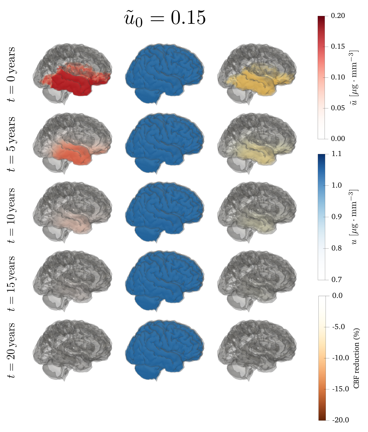
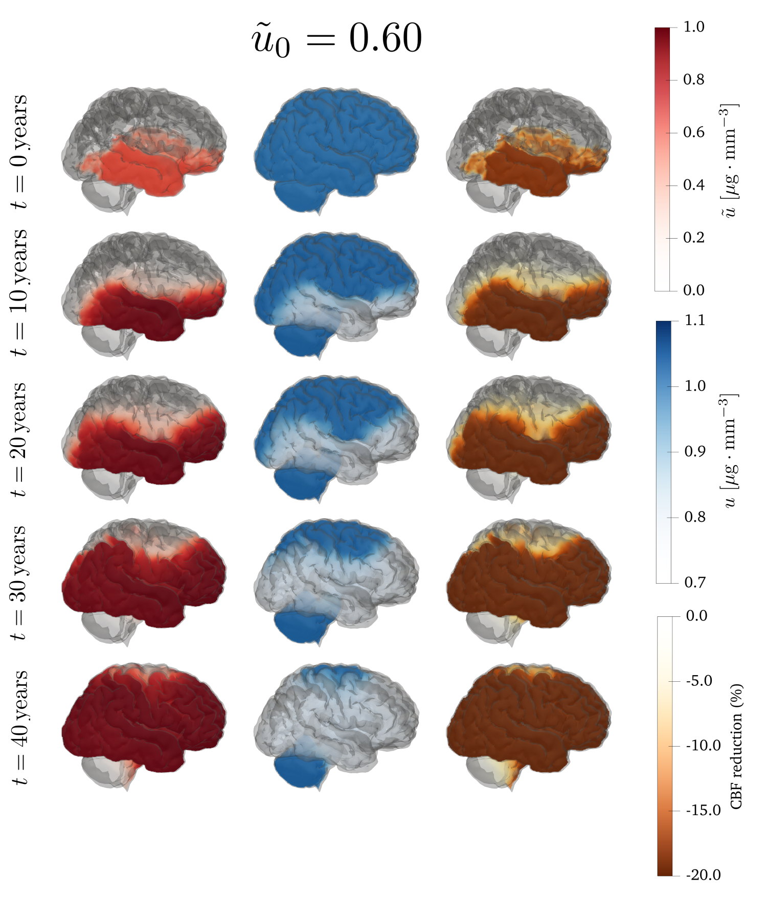
As in Test Case 1, we examine the impact of the initial pathogenic Aβ distribution on the model’s dynamics. Depending on its magnitude, an initial pathogenic seed can grow and spread like a wave through space or it can decay completely. Here, we simulate two initial conditions, one large and one small, both located in the basal temporal and orbitofrontal neocortex, , typical regions for the first phase of amyloid progression [24].
First, we test a small localized concentration of misfolded protein ( in ) with constant healthy protein throughout the domain. Figure 10(a) shows the result. Hypoperfusion in the temporal lobe—automatically induced by our initial condition—agrees with early AD literature [18]. The pathology does not develop: Aβ concentration decays, restoring the neocortex to the healthy equilibrium.
Next, we increase the seeding magnitude to in . As shown in Figure 10(b), this large initial seeding causes Aβ spreading through the cortical area, with associated neocortical hypoperfusion. This rise in misfolded proteins coincides with a local decrease in healthy protein population. The computed CBF rate drops by , consistent with the literature [38]. The spreading pattern first involves the temporal lobe [45], then diffuses to the upper cortex (occipital and frontal) [63], with the parietal lobe, brainstem, and cerebellum affected last—matching the stages in [24]. This reflects the spatial path length of the pathological wavefront.
5.2 Test Case 4: Injury-induced initiation of Aβ misfolding

As an extension of Test Case 2, we analyze the effect of an injured subdomain size on Aβ misfolding and spreading through the brain. We adopt the physical parameters from Appendix A (Table 2), except for
which induce injury in the frontal lobe of the left hemisphere. The hypoperfusion region is
with radii for mild, moderate, and severe injuries, respectively. Initial conditions are constant: and for healthy and misfolded proteins, respectively—representing a small perturbation from the healthy equilibrium. In Figure 11, we observe that already at the initial time , the parameters induce a significant reduction of the CBF rate in the injured region (approximately ) in all cases.


Figures 12 and 13 show the dynamics of misfolded and healthy protein concentrations, respectively. Moderate and severe injuries increase the pathogenic Aβ concentration () in the hypoperfused region, which then propagates through the frontal brain area—especially in the severe case. For the healthy Aβ concentration, we observe an initial concentration increase within the injured region, consistent with hypoperfusion-induced APP upregulation [27], followed by a decrease in concentration as the injured region switches to the diseased equilibrium, for which . Figure 11 shows an expansion of the hypoperfused region outward from the initial injury site in the severe and moderate cases, caused by the pathogenic Aβ distribution which induces vasoconstriction as it spreads.
In the mild injury case, the pathogenic Aβ concentration decays nearly vanishes within 5 years, while healthy protein shows slight upregulation to mitigate neuronal injury [27] (see Figures 12 and 13). The initial hypoperfusion region remains unchanged.
These results mirror those in Test Case 2. They reveal that hypoperfusive injury, if sufficiently severe, may be capable of inducing the outbreak of mixed Aβ –vascular pathology and its spatial invasion of otherwise healthy brain regions. This model behavior aligns with prior modelling work [1].
6 Conclusion
Alzheimer’s disease, the most common cause of dementia, is characterized by the accumumulation and spread of misfolded Aβ proteins in the brain, and is also associated with chronic cerebrovascular pathology [43]. The work presented here is motivated by the growing recognition of a positive feedback loop between Aβ accumulation and hypoperfusion in AD [29, 34, 38]. Our model describes the coupling between Aβ and cerebral blood flow (CBF) associated with Aβ-induced vascoconstriction [48, 64, 47] and hypoperfusion-induced modulation of Aβ metabolism [60, 59, 62, 71].
The model is similar in spirit to that of Ahern et al. [1], who assumed the same biological mechanisms. Whereas these authors used a network-based model of the brain and a semi-mechanistic model of blood flow within the network regions, the model presented here is continuous in space as well as in time, and its description of perfusion is based on multiple-network porous medium model. Interestingly, the emergent dynamics of the two models are qualitatively similar. Both exhibit multistability (Test Cases 1 and 3) and a capacity for vascular injury-induced disease outbreak (Test Cases 2 and 4), adding to the argument that these processes emerge generically.
From a numerical point of view, the differential equation has been discretized using a high-order discontinuous Galerkin method in space and implicit Euler time stepping in time. The model’s multistability was demonstrated for both idealized and realistic brain geometries. Moreover, we analyzed the possibility of describing the hypoperfusion-induction of the AD by introducing an initial hypoperfusion in the mathematical model. Finally, the numerical simulations on realistic brain geometries have been performed to highlight the importance of vascular–protein coupling in the mathematical description of AD pathology. Those simulations provided the typical spreading patterns of the pathology and confirmed the model quality in describing the physical phenomena.
6.1 Further developments and limitations
A limitation of the present model concerns the adoption of the heterodimer formulation, which provides a simplified description of Aβ kinetics and axonal transport. A natural extension of the present work would therefore be to enrich the reaction network by introducing additional compartments that distinguish between soluble oligomers, intermediate aggregates, and insoluble fibrils. Such multi-species models would allow us to explore state-dependent effects on clinical manifestations and comorbidities, and to represent more faithfully the different biological roles of the various aggregation states. There is no additional technical difficulty to include such effects but the real bottleneck is data availability for inference. As better data become available, it will be natural to introduce such effects.
As for the axonal transport, a purely diffusive operator cannot fully capture the directionality of axonal transport, which exhibits an anterograde–retrograde asymmetry and a concentration-dependent feedback of pathological tau. A possible further development would be to incorporate explicit advective transport through a reformulated model with motor-dependent velocity fields, as proposed in recent network transport models [49, 66].
Another promising extension would be the inclusion of additional aspects of Alzheimer’s disease pathology, such as brain atrophy, tau protein misfolding, and impaired clearance pathways. Within the proposed framework, not all model parameters are individually identifiable from currently available experimental and imaging data, in particular those associated with the coupling between the Aβ and perfusion models. Nevertheless, our numerical experiments indicate that the main desired qualitative features of the dynamics are captured by the simulations. A more systematic global sensitivity analysis, aimed at quantifying the relative influence of kinetic, vascular, and coupling parameters on key outcome measures, is an important direction for future work.
From a numerical perspective, an inherent drawback of the current model is its inability to automatically preserve the positivity of protein concentrations. The design of structure-preserving numerical schemes therefore represents a relevant avenue for future development. Moreover, a complete a priori analysis of the proposed numerical method would provide further theoretical insight into its stability and convergence properties. Finally, the introduction of local discontinuous Galerkin strategies could enhance the robustness of the numerical treatment, particularly in handling the nonlinear diffusion terms.
Finally, in the present formulation, anisotropy is solely based on the principal eigenvector of the diffusion tensor and does not explicitly account for tensor-shape descriptors. A more refined representation could exploit fractional anisotropy or shape indices, computed from the specific DWI data, to modulate the strength and directionality of anisotropic transport. Exploring such extensions is an interesting direction for future work.
Declaration of competing interests
The authors declare that they have no known competing financial interests or personal relationships that could have appeared to influence the work reported in this article.
Acknowledgments
OASIS-3 provided the brain MRI images: Longitudinal Multimodal Neuroimaging: Principal Investigators: T. Benzinger, D. Marcus, J. Morris; NIH P30 AG066444, P50 AG00561, P30 NS09857781, P01 AG026276, P01 AG003991, R01 AG043434, UL1 TR000448, R01 EB009352. AV-45 doses were provided by Avid Radiopharmaceuticals, a wholly-owned subsidiary of Eli Lilly.
Appendix A Parameter values for test cases
Tables 1 and 2 below report the parameter values used in the simulations of Sections 4 and 5, respectively.
| Parameter | Value | |
|---|---|---|
| Parameter | Value | |
|---|---|---|
| Dimensionless | Healthy | Misfolded |
|---|---|---|
| Parameter | Value | Value |
| Dimensionless | Healthy | Misfolded |
|---|---|---|
| Parameter | Value | Value |
| Parameter | Value | |
|---|---|---|
| Parameter | Value | |
|---|---|---|
| Dimensionless | Healthy | Misfolded |
|---|---|---|
| Parameter | Value | Value |
| Dimensionless | Healthy | Misfolded |
|---|---|---|
| Parameter | Value | Value |
References
- [1] (2025) Modelling cerebrovascular pathology and the spread of amyloid beta in Alzheimer’s disease. Proceedings of the Royal Society A: Mathematical, Physical and Engineering Sciences 481 (2311), pp. 20240548. External Links: Document Cited by: §1, §1, §2.1, §2.3, Remark 2.1, §4.2, §5.2, §6.
- [2] (1979) Continuum basis for diffusion in regions with multiple diffusivity. Journal of Applied Physics 50, pp. 1334. External Links: Document Cited by: §2.3.
- [3] (2023) A multi-scale model explains oscillatory slowing and neuronal hyperactivity in alzheimer’s disease. Journal of The Royal Society Interface 20 (198), pp. 20220607. Cited by: §1.
- [4] (2024) Discontinuous Galerkin approximations of the heterodimer model for protein-protein interaction. Computer Methods in Applied Mechanics and Engineering 431, pp. 117282. External Links: Document Cited by: Table 2, Table 2, §1, §1, §3.1, §3.2, §4.1.
- [5] (2026) Polytopal mesh agglomeration via geometrical deep learning for three-dimensional heterogeneous domains. Mathematics and Computers in Simulation 241, pp. 335–353. External Links: Document Cited by: §1.
- [6] (2016) High order discontinuous Galerkin methods on simplicial elements for the elastodynamics equation. Numerical Algorithms 71, pp. 181–206. External Links: Document Cited by: §1.
- [7] (2018) High-order Discontinuous Galerkin methods for the elastodynamics equation on polygonal and polyhedral meshes. Computer Methods in Applied Mechanics and Engineering 342, pp. 414–437. External Links: Document Cited by: §1.
- [8] (2017) Alzheimer’s disease: a mathematical model for onset and progression. Mathematical medicine and biology : a journal of the IMA 34 (2), pp. 193–214. External Links: Document Cited by: §1.
- [9] (2024) The role of clearance in neurodegenerative diseases. SIAM Journal on Applied Mathematics 84 (3), pp. S172–S198. External Links: Document Cited by: §1, §1.
- [10] (2022) Human intracranial pulsatility during the cardiac cycle: a computational modelling framework. Fluids and Barriers of the CNS 19, pp. 84. External Links: Document Cited by: §1.
- [11] (2025) Personalised regional modelling predicts tau progression in the human brain. PLoS Biology 23 (7), pp. e3003241. Cited by: §1, §2.1.
- [12] (2023) Numerical modeling of the brain poromechanics by high-order discontinuous Galerkin methods. Mathematical Models and Methods in Applied Sciences 33 (08), pp. 1577–1609. External Links: Document Cited by: §1, §1, §2.2, §3.1, §5.
- [13] (2024) Uncertainty quantification for Fisher-Kolmogorov equation on graphs with application to patient-specific Alzheimer’s disease. ESAIM: Mathematical Modelling and Numerical Analysis 58 (6), pp. 2135–2154. External Links: Document Cited by: §1, §1, §2.1.
- [14] (2024) Structure preserving polytopal discontinuous Galerkin methods for the numerical modeling of neurodegenerative diseases. Journal of Scientific Computing 100 (2), pp. 39. External Links: Document Cited by: §1.
- [15] (2023) Discontinuous Galerkin methods for Fisher–Kolmogorov equation with application to α-synuclein spreading in Parkinson’s disease. Computer Methods in Applied Mechanics and Engineering 417, pp. 116450. External Links: Document Cited by: §1, §2.1.
- [16] (2024) Exploring tau protein and amyloid-beta propagation: a sensitivity analysis of mathematical models based on biological data. Brain Multiphysics 7, pp. 100098. External Links: Document Cited by: §1, §1, §2.1, Remark 2.1, §4.1.
- [17] (2019) Neutrophil adhesion in brain capillaries reduces cortical blood flow and impairs memory function in Alzheimer’s disease mouse models. Nature Neuroscience 22 (3), pp. 413–420. External Links: Document Cited by: §1.
- [18] (1992) Reduced temporal lobe blood flow in Alzheimer’s disease. Neurobiology of Aging 13 (4), pp. 483–491. External Links: Document Cited by: §5.1.
- [19] (2016) Cerebral blood flow and autoregulation: current measurement techniques and prospects for noninvasive optical methods. Neurophotonics 21 (3), pp. 031411. External Links: Document Cited by: §5.
- [20] (2012) FreeSurfer. NeuroImage 62 (2), pp. 774–781. External Links: Document Cited by: §5, §5.
- [21] (2019) Prion-like spreading of Alzheimer’s disease within the brain’s connectome. Journal of The Royal Society Interface 16 (159), pp. 20190356. External Links: Document Cited by: §1, §1, §4.1, §5.1.
- [22] (2020) Spatially-extended nucleation-aggregation-fragmentation models for the dynamics of prion-like neurodegenerative protein-spreading in the brain and its connectome. Journal of Theoretical Biology 486, pp. 110102. Cited by: §1.
- [23] (2016) From a microscopic to a macroscopic model for Alzheimer disease: two-scale homogenization of the Smoluchowski equation in perforated domains. Journal of Nonlinear Science 24, pp. 717–753. External Links: Document Cited by: §1.
- [24] (2015) Alzheimer’s and Parkinson’s diseases: The prion concept in relation to assembled A, tau, and -synuclein. Science 349, pp. 1255555. External Links: Document Cited by: §1, §5.1, §5.1.
- [25] (2011) Vascular contributions to cognitive impairment and dementia: A statement for healthcare professionals from the American Heart Association/American Stroke Association. Stroke 42 (9), pp. 2672–2713. External Links: Document Cited by: §4.2.
- [26] (2020) Neuronal oscillations on evolving networks: dynamics, damage, degradation, decline, dementia, and death. Physical Review Letters 125 (12), pp. 128102. Cited by: §1.
- [27] (2017) APP as a protective factor in acute neuronal insults. Frontiers in Molecular Neuroscience 10, pp. 22. External Links: Document Cited by: §1, §5.2, §5.2.
- [28] (2013) The pathobiology of vascular dementia. Neuron 80 (4), pp. 844–866. External Links: Document Cited by: §1.
- [29] (2004) Neurovascular regulation in the normal brain and in Alzheimer’s disease. Nature Reviews Neuroscience 5 (5), pp. 347–360. External Links: Document Cited by: §1, §6.
- [30] (2016) Early role of vascular dysregulation on late-onset Alzheimer’s disease based on multifactorial data-driven analysis. Nature Communications 7, pp. 11934. External Links: Document Cited by: §1.
- [31] (2021) On the sensitivity analysis of porous finite element models for cerebral perfusion estimation. Annals of Biomedical Engineering 49 (12), pp. 3647–3665. External Links: Document Cited by: §1, §2.2.
- [32] (2021) A porous circulation model of the human brain for in silico clinical trials in ischaemic stroke. Interface Focus 11, pp. 20190127. External Links: Document Cited by: Table 2, Table 2, §1, §2.2, §2.2, §2.3, §5, §5.
- [33] (2023) MRI-based parameter inference for cerebral perfusion modelling in health and ischaemic stroke. Computers in Biology and Medicine 166, pp. 107543. External Links: Document Cited by: §1, §2.2, §2.3.
- [34] (2012) Does vascular pathology contribute to Alzheimer changes?. Journal of the Neurological Sciences 322 (1-2), pp. 141–147. External Links: Document Cited by: §1, §6.
- [35] (2021) Biology in time and space: a partial differential equation modeling approach. Vol. 50, American Mathematical Soc.. Cited by: §4.1.
- [36] (2020) Anisotropic diffusion and traveling waves of toxic proteins in neurodegenerative diseases. Physics Letters A 384 (36), pp. 126935. Cited by: §1.
- [37] (2017) Cerebral blood flow regulation and neurovascular dysfunction in Alzheimer disease. Nature Reviews Neuroscience 18 (7), pp. 419–434. External Links: Document Cited by: §1, §4.2.
- [38] (2020) Cerebral blood flow decrease as an early pathological mechanism in Alzheimer’s disease. Acta Neuropathologica 140 (6), pp. 793–810. External Links: Document Cited by: §1, §2.3, §2.3, §5.1, §6.
- [39] (2019) OASIS-3: Longitudinal neuroimaging, clinical, and cognitive dataset for normal aging and Alzheimer disease. External Links: MedRxiv, Document Cited by: §5.
- [40] (2019) A mixed finite element method for nearly incompressible multiple-network poroelasticity. SIAM Journal on Scientific Computing 41 (2), pp. A722–A747. External Links: Document Cited by: §1, §1.
- [41] (2025) A -adaptive polytopal discontinuous galerkin method for high-order approximation of brain electrophysiology. Computer Methods in Applied Mechanics and Engineering 446, pp. 118249. External Links: Document Cited by: §1.
- [42] (2023) A computational study of fluid transport characteristics in the brain parenchyma of dementia subtypes. Journal of Biomechanics 159, pp. 111803. External Links: Document Cited by: §1.
- [43] (2016) Cerebrovascular disease in ageing and Alzheimer’s disease. Acta Neuropathologica 131 (5), pp. 645–658. External Links: Document Cited by: §4.2, §6.
- [44] (2022) Mathematical Modeling of the Human Brain: From Magnetic Resonance Images to Finite Element Simulation. Vol. 10, Springer International Publishing. External Links: Document Cited by: §2.1, §5.
- [45] (2017) Tau and -Amyloid are associated with medial temporal lobe structure, function, and memory encoding in normal aging. The Journal of Neuroscience 37 (12), pp. 3192–3201. External Links: Document Cited by: §5.1.
- [46] (2006) Diffusion versus network models as descriptions for the spread of prion diseases in the brain. Journal of Theoretical Biology 240 (1), pp. 104–113. External Links: Document Cited by: §1.
- [47] (2001) A-peptides enhance vasoconstriction in cerebral circulation. American Journal of Physiology - Heart and Circulatory Physiology 281 (6), pp. 2417–2424. External Links: Document Cited by: §1, §2.3, §6.
- [48] (2019) Amyloid oligomers constrict human capillaries in Alzheimer’s disease via signaling to pericytes. Science 365 (6450), pp. eaav9518. External Links: Document Cited by: §1, §2.3, §2.3, §6.
- [49] (2026) A multiscale theory for network advection-reaction-diffusion: h. oliveri et al.. Journal of Mathematical Biology 92 (5), pp. 65. Cited by: §6.1.
- [50] (2025) A coupled mathematical and numerical model for protein spreading and tissue atrophy applied to Alzheimer’s disease. Computer Methods in Applied Mechanics and Engineering 444, pp. 118118. External Links: Document Cited by: §1, §1.
- [51] (2018) Multiscale modelling of blood flow in cerebral microcirculation: details at capillary scale control accuracy at the level of the cortex. Plos One 13 (1), pp. e0189474. External Links: Document Cited by: §2.3.
- [52] (2021) Parameter robust preconditioning by congruence for multiple-network poroelasticity. SIAM Journal on Scientific Computing 43, pp. B984–B1007. External Links: Document Cited by: §1, §1.
- [53] (1991) Molecular biology of prion diseases. Science 252 (5012), pp. 1515–1522. External Links: Document Cited by: §2.1.
- [54] (2004) Atherosclerosis of cerebral arteries in Alzheimer disease. Stroke 35 (11 suppl. 1), pp. 2623–2627. External Links: Document Cited by: §4.2, §4.2.
- [55] (2012) Neurovascular dysfunction and faulty amyloid -peptide clearance in Alzheimer disease. Cold Spring Harbor Perspectives in Medicine 2 (10), pp. 1–18. External Links: Document Cited by: §4.2.
- [56] (2019) The interplay of biochemical and biomechanical degeneration in Alzheimer’s disease. Computer Methods in Applied Mechanics and Engineering 352, pp. 369–388. External Links: Document Cited by: §1.
- [57] (2021) Alzheimer’s disease. The Lancet 397, pp. 1577–1590. External Links: Document Cited by: §1.
- [58] (2017) Depth-dependent flow and pressure characteristics in cortical microvascular networks. PLOS Computational Biology 13 (2), pp. e1005392. External Links: Document Cited by: §5.
- [59] (2000) Hypoperfusion induces overexpression of β-amyloid precursor protein mRNA in a focal ischemic rodent model. Brain Research 853 (1), pp. 1–4. External Links: Document Cited by: §1, §2.3, §6.
- [60] (1998) Estrogen attenuates over-expression of β-amyloid precursor protein messager RNA in an animal model of focal ischemia. Brain research 810 (1-2), pp. 87–92. External Links: Document Cited by: §6.
- [61] (2015) Vascular contributions to cognitive impairment and dementia including Alzheimer’s disease. Alzheimer’s and Dementia 11 (6), pp. 710–717. External Links: Document Cited by: §4.2.
- [62] (2006) Hypoxia facilitates Alzheimer’s disease pathogenesis by up-regulating BACE1 gene expression. Proceedings of the National Academy of Sciences 103 (49), pp. 18727–18732. External Links: Document Cited by: §1, §2.3, §6.
- [63] (2022) Phases of a beta-deposition in the human brain and its relevance for the development of AD. Neurology 58 (12), pp. 1791–1800. External Links: Document Cited by: §5.1.
- [64] (1996) -Amyloid-mediated vasoactivity and vascular endothelial damage. Nature 380 (6570), pp. 168–171. External Links: Document Cited by: §1, §2.3, §6.
- [65] (2020) Protein-protein interactions in neurodegenerative diseases: A conspiracy theory. PLOS Computational Biology 16 (10), pp. e1008267. External Links: Document Cited by: §1, §1.
- [66] (2025) A network-level transport model of tau progression in the Alzheimer’s brain. Mathematical Medicine and Biology: A Journal of the IMA 42 (2), pp. 212–238. External Links: Document Cited by: §6.1.
- [67] (2011) Cerebral water transport using multiple-network poroelastic theory: application to normal pressure hydrocephalus. Journal of Fluid Mechanics 667, pp. 188–215. External Links: Document Cited by: §1, §2.2, §2.3.
- [68] (2020) Exploring neurodegenerative disorders using a novel integrated model of cerebral transport: Initial results. Proceedings of the Institution of Mechanical Engineers, Part H: Journal of Engineering in Medicine 234 (11), pp. 1223–1234. External Links: Document Cited by: §1, §1.
- [69] (2019) A physics-based model explains the prion-like features of neurodegeneration in Alzheimer’s disease, Parkinson’s disease, and amyotrophic lateral sclerosis. Journal of the Mechanics and Physics of Solids 124, pp. 264–281. External Links: Document Cited by: §1, §2.1, §4.1, §5.1.
- [70] (2018) Multiphysics of prionlike diseases: Progression and atrophy. Physical Review Letters 121 (15), pp. 158101. External Links: Document Cited by: §1, §2.1.
- [71] (2007) Hypoxia-inducible factor 1α (HIF-1α)-mediated hypoxia increases BACE1 expression and β-amyloid generation. Journal of Biological Chemistry 282 (15), pp. 10873–10880. External Links: Document Cited by: §2.3, §6.
- [72] (2011) Neurovascular pathways to neurodegeneration in Alzheimer’s disease and other disorders. Nature Reviews Neuroscience 12 (12), pp. 723–738. External Links: Document Cited by: §1, §4.2.