Spacetime Quasi-normal Mode Oscillations of Anisotropic Neutron Stars
Abstract
Neutron star asteroseismology offers a unique opportunity to probe nuclear physics through stellar oscillations. Although the pressure inside of a neutron star is typically assumed to be isotropic, pressure anisotropy can arise from various physical mechanisms, including elasticity, viscosity, and magnetic fields. Previous studies of nonradial stellar quasi-normal mode oscillations with anisotropic pressure have focused primarily on fluid modes. In this paper, we compute, for the first time, spacetime oscillation modes (so-called -modes) of anisotropic neutron stars. Using a perturbative framework for stellar oscillations with pressure anisotropy, developed previously by some of the authors, together with a phenomenological anisotropy model, we find that both the real and imaginary parts of the -mode frequencies decrease as the tangential pressure becomes dominant over the radial pressure. Although we do not find any unstable -modes within the physically viable parameter space, unstable -modes appear in an unphysical branch of solutions when the tangential pressure strongly dominates the radial one. We also find that the relation between the real part of the -mode frequency and the stellar compactness is quasi-universal with respect to variations in the equation of state and the degree of pressure anisotropy. In contrast, the relation between the imaginary part of the -mode frequency and the stellar compactness depends on the degree of anisotropy, but remains equation-of-state universal when the anisotropy is fixed. Finally, we discuss potential mode crossings and the validity of certain approximations that have been shown to work well for -mode calculations in the isotropic case.
I Introduction
Neutron stars (NSs) are extremely compact objects whose central density exceeds the nuclear saturation density and thus provide an ideal laboratory environment for probing nuclear physics. Various NS observations through radio [Antoniadis:2013pzd, NANOGrav:2019jur, Saffer:2024tlb], x-rays [Raaijmakers:2021uju, Yunes:2022ldq], gamma-rays [Guedes:2024zkh], and gravitational waves [LIGOScientific:2018cki, Chatziioannou:2020pqz, Yunes:2022ldq] have placed constraints on the equation of state (EOS) for nuclear matter, the relation between energy density and pressure.
One useful approach for extracting nuclear physics information from NSs is stellar seismology [Andersson:1996pn, Andersson:1997rn, Kokkotas:1999bd], the study of oscillations of astronomical objects. The nonradial oscillation modes of NSs are quasi-normal modes, characterized by complex frequencies due to damping over time via gravitational wave emission. These quasi-normal modes carry information about nuclear physics through their dependence on the interior properties of NSs, which are governed by the underlying EOS of nuclear matter. Quasi-normal modes can be classified based on the major restoring forces or properties of the composite waves, including the fundamental mode (-mode), the pressure mode (-mode), and the spacetime mode (-mode) [Kokkotas:1999bd].
Quasi-normal modes are also useful for studying the (non-radial) stability of stellar modes. Stellar oscillations are conventionally described by containing a time-dependent oscillation function, , where is the frequency and is the time. A stellar oscillation mode is considered stable if the complex frequency of the quasi-normal mode has a positive imaginary part such that is exponentially decaying. Detweiler and Ipser [ipser1973] have developed a method that argues the stability of quasi-normal modes through a variational method. They found that all spherically symmetric equilibrium, isotropic NSs with a positive density, positive pressure, negative density gradient, and non-negative Schwarzschild discriminant have stable quasi-normal modes111Convective instability can still occur via a negative Schwarzschild discriminant..
Most studies on NSs focus on isotropic pressure, while some degree of anisotropy in pressure may exist inside NSs. Such anisotropy can arise from different origins, including viscosity [viscosity], elasticity [elasticity, Karlovini:2002fc, Dong:2024lte], superconductivity [HERRERA199753], and strong magnetic field [Most_2025]. Pressure anisotropy also exists in solutions to the Einstein equations for exotic compact objects, such as boson stars [Macedo:2013jja], gravastars [Chirenti_2007, Cattoen_2005], and dark energy stars [lopes].
There are several studies on non-radial oscillations for anisotropic NSs. These modes were first calculated within the Cowling approximation [Cowling:1941nqk], where only fluid perturbations are kept while spacetime perturbations are ignored. It is only recently that the complete perturbative framework for computing non-radial oscillations for anisotropic NSs has been developed in full general relativity [nonradial] (see [Mondal:2023wwo, Mondal:2023wwo, Arbanil:2025jep] for related works). In this reference, some of us computed the -modes and -modes of NSs with some phenomenological anisotropy models and found that, unlike isotropic NSs, anisotropic NS -modes can become unstable. They justified this numerical finding with some analytic calculations by extending the variation principle method by Detweiler and Ipser [ipser1973] to anisotropic NSs, proving that the modes can become unstable once the anisotropy is turned on.
A recent work [Guedes:2025gqi] by some of us studied quasi-universal relations between the real part of the -mode frequency and the tidal deformability for anisotropic NSs, which was known to exist for isotropic NSs [Chan:2014kua] (see e.g. [Yagi:2015hda] for another work on quasi-universal relations for anisotropic NSs). For the anisotropic case, we found that the relations depend strongly on the amount of anisotropy, while they remain EOS-insensitive for a fixed anisotropy. Using these relations, together with the inference on the -mode frequency and the tidal deformability of the binary NS merger event GW170817 [Pratten:2019sed], we derived EOS-insensitive bounds on anisotropy.
One type of oscillation mode for anisotropic NSs that has not been computed previously is the -mode [1992MNRAS.255..119K, Andersson_1996]. -modes are also known as spacetime modes since they originate from the metric perturbations, so they cannot be computed under the Cowling approximation. Thanks to the recent development of the perturbative framework for stellar oscillations with pressure anisotropy in full general relativity [nonradial], we are now able to compute, for the first time, polar -mode oscillations for anisotropic NSs, which is the goal of this paper. We solve the same perturbation equations in [nonradial] that we used to compute -modes and -modes. In contrast to the fluid modes (-modes and -modes, etc.) which have an imaginary part of the frequency that is orders of magnitude smaller than the real part, -mode frequencies have comparable imaginary and real parts. Therefore, we use Leaver’s continued fraction method [1985Leaver] to compute the -mode frequencies.
Figure 1 summarizes our main result, which presents the -mode frequencies as a function of the anisotropy parameter , defined in Eq. \eqrefeq:anisotropy_model, for a selected EOS and central density. The dimensionless anisotropy parameter denotes the extent of pressure difference between the radial and tangential directions, where corresponds to the isotropic case while means that the tangential pressure dominates the radial one. The blue branches are for physically viable models, while the red ones are for unphysical models that violate causality and positivity of the tangential pressure for this specific choice of parameters (other physicality conditions can be violated for other choices of parameters). First, observe that both the real and imaginary parts of the -mode frequency decrease as we decrease the anisotropy parameter . Second, although we did not identify any unstable modes within the physically-viable branch, -modes can become unstable for unphysical models with largely negative values of the anisotropy parameter. The analytic argument in [nonradial] for potential mode instabilities for anisotropic NSs did not specify the type of modes, and hence, it applies to the unstable -modes found here.

Are there any quasi-universal relations for -mode frequencies that are insensitive to EOSs? For isotropic NSs, both real and imaginary frequencies enjoy universal relations with the stellar compactness [Benhar:2004xg, TL, Tsui:2005zf]. For anisotropic NSs, we found that the relation between the real part of the -mode frequency and compactness remain quasi-universal against variations in both EOSs and the anisotropy parameter . On the other hand, the relation between the imaginary part of the -mode frequency and compactness depends sensitively on , while it remains EOS-insensitive for fixed . The latter is similar to the relation between the -mode frequency and tidal deformability mentioned earlier [Guedes:2025gqi].
The rest of the paper is organized as follows. In Sec.II we review how to construct background solutions and the perturbative framework for computing stellar oscillations with pressure anisotropy. In Sec. III, we provide the phenomenological anisotropy model and present numerical results for both background solutions as well as -mode frequencies. We conclude in Sec. IV and give some discussions, including potential mode crossing and the validity of certain approximations for computing -mode frequencies that are known to work well for isotropic NSs [Andersson_1996, Wu_2007].
II Perturbation framework
In this section, we review the perturbative framework for computing -mode oscillations for anisotropic NSs following [nonradial] (see [Mondal:2023wwo, Mondal:2025ixk, Arbanil:2025jep] for related works). We first describe how to construct a spherically-symmetric background configuration in units. The line element is given by
| (1) |
with
| (2) |
The stress energy tensor for the anisotropic fluid is given by [1974StressEnergyTensor]
| (3) |
Here, and , where is the four velocity of the fluid element, and is the unit radial vector perpendicular to . and are the energy density and the radial pressure, while is the pressure anisotropy between the radial and tangential directions.
Now, we can solve the NS perturbation background variables. Plugging the above line element and the stress-energy tensor into the Einstein equations, one finds a set of modified Tolman-Oppenheimer-Volkoff (TOV) equations for anisotropic stars [Horvat_2011]:
{align}
m’=4πr^2ρ,
ν’=2m+4 πr3prr2e^λ,
p_r’=-(ρ+p_r)ν’2-2σr.
Here, a prime denotes a radial derivative, and is defined as which corresponds to the mass enclosed within a sphere of radius .
Let us now introduce a linear perturbation to both the gravity and matter sectors. The metric is perturbed as
| (4) |
with
| (10) | |||||
where are spherical harmonics in spherical coordinates and is the angular frequency of the perturbation.
To study perturbations to the anisotropic fluid, we introduce the fluid displacement vector as [nonradial]
{align}
ζ^r = W(r)r eλ(r)/2Y_ℓm(θ,ϕ) e^iωt,
ζ^θ= V(r)r2 ∂_θY_ℓm (θ,ϕ) e^iωt,
ζ^ϕ= V(r)r2sin2θ ∂_ϕY_ℓm (θ,ϕ) e^iωt.
We then arrive at the perturbation equations from the perturbed Einstein equations,
| (11) |
and the perturbed equation of motion,
| (12) |
The anisotropic perturbation equations are derived from the Einstein field equations and matter equations of motion as in [nonradial] (see Appendix A). We follow the general method as described in [LD]. To solve the frequency of the oscillation mode, we first solve for the stellar background by integrating the modified TOV equation. After that, we observe that the above set of equations establish an initial value problem with the vector function
| (13) |
For a given oscillation frequency , we can solve the perturbation functions throughout the star. Finally, we use Leaver’s continued fraction method [1985Leaver, Sotani:2001bb].
III Numerical Results
In this section, we provide details of the procedure for our numerical calculations and their results. We adopt the same anisotropy model as in [nonradial, Guedes:2025gqi] that is an extension of the model used in [Horvat_2011]. The pressure difference between the radial and the tangential directions is given by {align} σ= βp_r μ^2, where and is the dimensionless anisotropy parameter.
For equations of state (EOSs) connecting the radial pressure and energy density, we use the following: WFF1, SLy4, and MS1. WFF1 (MS1) is a soft (stiff) EOS, while SLy4 is in between.
III.1 Spherically-symmetric NSs with Pressure Anisotropy
We begin by constructing anisotropic NSs with spherically-symmetric configurations, which will be used as background solutions when considering stellar perturbations in the subsequent subsection.
To achieve this, we solve the anisotropic TOV equations in Eqs. \eqrefeq:m_TOV and \eqrefeq:pr_TOV numerically. The boundary conditions at (where represents the stellar radius) near the stellar center
are given by
{align}
p_r = p_c + O(r_0^2),
ρ= ρ_c + O(r_0^2),
m = 4π3 ρ_c r_0^3+ O(r_0^5).
For a chosen central pressure or central energy density , we use the above asymptotic behaviors to solve Eqs. \eqrefeq:m_TOV and \eqrefeq:pr_TOV. The radius is determined from the condition while the stellar mass is defined as . Eq. \eqrefeq:nu_TOV for is then solved under the boundary condition
| (14) |
Figure 2 presents the mass-radius relation for anisotropic NSs. Observe that the NS radius and maximum mass increase (decrease) for negative (positive) from the isotropic case. Similarly to the isotropic case [Tassoul1978], stars with the anisotropy model in Eq. \eqrefeq:anisotropy_model become unstable after reaching the maximum mass as one increases the central energy density [Guedes:2025gqi].
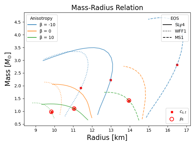

Below, we only consider stellar configurations that are physically viable, i.e. those that respect the energy conditions, positivity of pressure, and causality [Guedes:2025gqi]:
1. weak energy condition [Poisson:2009pwt]: ρ≥0, ρ+p_r¿0, ρ+p_t¿0,
2. null energy condition [Poisson:2009pwt]: ρ+p_r≥0 ρ+p_t≥0,
3. strong energy condition [Poisson:2009pwt]: ρ+p_r+2p_t≥0, ρ+p_r≥0, ρ+p_t≥0,
4. dominant energy condition [Poisson:2009pwt]: ρ≥0, ρ≥—p_r—, ρ≥—p_t—,
5. positivity of pressure: p_r≥0, p_t≥0,
6. causality: 0 ≤c^2_s,r, c^2_s,t ≤1.
Here is the central density while and are the speed of sound in the radial and tangential directions, defined by {align} c_s,r^2=(∂pr∂ρ)_eq, c_s,t^2=(∂pt∂ρ)_eq, where the subscript “eq” denotes the derivative of the background against .
Some of these requirements are naturally satisfied for a NS. They include: {align} ρ≥0, ρ+p_r≥0, p_r≥0, c_s,r^2≥0, and, if is satisfied, and are also satisfied.
Let us further reduce some redundant constraints. Consider a star that has at a certain point inside the star. At the star surface, the radial and tangential pressure must be zero. Therefore, there must exist a point at which the negative tangential pressure increases (or decreases in magnitude) as the radius increases. Since our star generally has , this implies that there exists a point at which . Therefore, a violation of the positive tangential pressure condition must also violate the tangential causality condition.
As a result, the criteria that we are left with are
{align}
dMdρc≥0,
ρ≥—p_r—, ρ≥—p_t—,
1≥c_s,r^2, c_s,t^2≥0.
The maximum-mass criterion holds for anisotropic stars using the modified H-model, i.e. stars such that are radially stable [Guedes:2025gqi]. The dominant energy condition generally holds for the range of anisotropy, EOS, and central density that we are studying, except for very few models. Radial stability and tangential causality constraints on the NS mass are shown in Fig. 3. For a fixed EOS and anisotropy, the allowed mass range corresponds to the region below the curve that gives the smaller maximum mass limit.
III.2 -modes
Having spherically-symmetric configurations explained in Sec. III.1 as background, we next study stellar perturbations to find -modes for anisotropic NSs.
III.2.1 Numerical Procedures
We need to solve an eigenvalue problem to find the -mode oscillation frequency . The eigenvector in Eq. \eqrefeq:eigen_vec has an arbitrary magnitude as it satisfies homogeneous equations, and we care only about its direction. We can solve this vector function with initial conditions from the center of the star and boundary conditions at the surface of the star. At the center of the star, we require the following regularity condition:
| (15) |
This gives the relation of initial values at :
{align}
H_1(0)=16πℓ(ℓ+1) (ρ_0+p_0) W(0)+2l(ℓ+1)K(0) ,
X(0)= e^ν_0/2(ρ_0+p_0) (4π3 ρ_0+4πp_0-ω2eν0ℓ+K(0)2),
where
{align}
K(0)=±(ρ_0+p_0),
W(0)=1,
give the two linearly independent solutions.
The surface boundary condition requires the Lagrangian perturbation of the pressure to vanish. Since is proportional to the Lagrangian perturbation of the radial pressure, as in Eq. (A7) in [nonradial], we choose three independent boundary conditions at the stellar radius :
| (16) |
Note that the choices of the numerical values in are arbitrary as long as they are linearly independent and satisfy . The actual dimensions of the perturbation variables are carried by the coefficients in Eq. \eqrefeq:a_coefficients. We solve the perturbation equations numerically from the center to using two independent vectors, labeled , and we also solve backward from the surface to using three independent vectors, labeled . We match the five solutions at by
| (17) |
to determine the coefficients . This would give us the solution to the perturbation equations throughout the star normalized by . From the perturbation vector at the surface of the star, we can follow Leaver’s method [1985Leaver] to solve the quasi-normal mode frequencies.
III.2.2 Results
We now present our numerical findings on the -modes for anisotropic NSs. Figure 4 presents the real and imaginary parts of the -mode frequency against the anisotropy parameter for three different EOSs with two different central energy densities . Observe that both the real and imaginary frequencies increase as one increases the anisotropy. Similarly to the isotropic case, the real and imaginary parts of the frequencies are higher for softer EOSs and lower .


The -mode frequencies have been found to enjoy quasi-universal relations for isotropic NSs [Benhar:2004xg, TL, Tsui:2005zf]. Let us now study whether such universality holds even for anisotropic NSs. Figure 5 presents the real and imaginary parts of the -mode scaled frequencies, , against the stellar compactness for various EOSs and anisotropy parameters. We also show the fit in [TL] for isotropic NSs. For the real frequency, observe that the relation found for isotropic NSs is approximately valid even for anisotropic NSs. Namely, the relation is quasi-universal to variation in both EOSs and anisotropy. On the other hand, the relations with the imaginary frequency have a clear anisotropy dependence. Interestingly, the relations remain insensitive to the EOS (i.e. relations) for fixed anisotropy. The latter is similar to the quasi-universal relation between the fundamental mode frequency and the tidal deformability for anisotropic NSs found in [Guedes:2025gqi]. One can further eliminate the compactness dependence to find the relation between the real and imaginary parts of the -mode frequencies, as shown in Fig. 6. Similar to the relation between the imaginary frequency and compactness, the relations have a significant anisotropy dependence, while they remain EOS-insensitive for fixed anisotropy.


We next study the stability of -modes for anisotropic NSs, which can be checked from the sign of . Namely, the mode becomes stable (unstable) if is positive (negative). Within the physically-viable parameter space for our anisotropic NS models, we did not find any unstable -modes. On the other hand, we identified unstable -modes once we relax some of the physically-viable conditions, i.e. the causality on the tangential sound speed for the specific parameters we chose.
Figure 1 presents the -mode frequency against the anisotropy parameter for NSs with MS1 EOS and the central energy density of g/cm3. For , NSs are not physically viable as the tangential sound speed can exceed unity. For the above EOS and central density, we found that can go negative when , indicating that -modes become unstable for such unphysical NSs with largely-negative (i.e. tangential pressure dominated) anisotropy.
IV Conclusions and Discussions
In this work, we computed, for the first time, -mode oscillations for anisotropic NSs following the perturbation framework in full general relativity developed in [nonradial] by some of the authors. For the phenomenological anisotropy model used in [nonradial, Guedes:2025gqi] that is an extension of the one proposed by Horvat et al. [Horvat_2011], we found the real and imaginary parts of the -mode frequencies to increase as the anisotropy parameter increases for a fixed central density. We found the relation between and to be insensitive to both EOS and the anisotropy . On the other hand, the one between and depends sensitively on while it remains almost EOS-universal for a fixed . We did not identify any unstable -modes within the physically-viable parameter space, while the modes can be unstable for largely-negative when we consider unphysical parameter regions. In [nonradial], we found that -modes can be unstable for anisotropic stars with the same phenomenological model as considered here, and provided an analytic justification on why the modes can be unstable for non-vanishing anisotropy through a variation method following [ipser1973] for isotropic NSs. Such an analysis applies to all polar modes, and hence, our finding of unstable -modes for anisotropic NSs is consistent with the analysis in [nonradial].
There is a possibility that the unstable mode we found may not correspond to -modes in our original classification scheme at less negative , as the mode may have encountered an avoided crossing with other modes when we decrease . The sharp change in slope of the real frequencies in Figs. 1 and 7 may be due to a close encounter of the -mode with another quasi-normal mode. In classical stellar pulsation theory, the oscillation frequency of each mode can be viewed as a smooth function of a varying parameter (e.g. the anisotropy parameter or the stellar compactness ). When the parameter varies, the eigenfrequencies of these modes may approach each other. If the modes are coupled with each other, or equivalently, they do not originate from completely decoupled wave equations, the mode frequencies will repel each other to avoid a crossing. The mode characteristics will be exchanged as the eigenfrequencies of the two modes move away from the point of closest approach. This feature is well-known in Hermitian eigenvalue problems and has been identified in classical stellar pulsations (see, e.g., [1977A&A]). In non-Hermitian systems, the situation is more complicated as there can be avoided crossings in real frequency and true crossings in the imaginary frequency, or the other way round [Rotter_2009_arxiv, Rotter_2009]. Further studies are required to uncover the mode-coupling properties of the -mode with the other modes. That requires a thorough search of all quasi-normal modes at nearby frequencies, which we shall leave as future work. Here, we simply assume an exchange in mode characteristics after an avoided crossing occurs for the real frequency, similar to the case found between the -mode and shear modes in a solid relativistic star [Lau2017thesis]. Figure 7 shows the rescaled -mode frequency as a function of the compactness. Observe that the real part of the frequency does not seem to connect smoothly from the physical branch to the unphysical branch as the compactness increases, which may indicate the presence of avoided crossing. Thus, the unstable mode we have discovered in the unphysical branch may be the result of the avoidance of crossing from another mode.

Previous works have explored the possibility of reducing the complexity of -modes through approximations. In Appendix LABEL:sec:ICA, we discuss two approximations of -modes, inverse Cowling approximation (ICA) [Andersson_1996] and generalized inverse Cowling approximation (GICA) [Wu_2007]. We also discussed the validity of ICA and GICA for anisotropic NSs.
More work is needed to arrive at more robust conclusions on mode crossing and the validity of GICA on -modes for anisotropic NSs. It would also be important to study anisotropic models other than the one considered here, in particular, for models that are more physically motivated, such as the ones for elastic NSs [Dong:2024lte] or those modeled based on liquid crystal [Cadogan:2024mcl, Cadogan:2024ohj, Cadogan:2024ywc]. We leave these studies for future work.
Acknowledgements.
V.G., S.A. and K.Y. acknowledge support from the Owens Family Foundation. S.A. and K.Y. also acknowledge support from NSF Grant PHY-2309066 and PHY-2339969. S.Y.L. acknowledges support from Montana NASA EPSCoR Research Infrastructure Development under award No. 80NSSC22M0042.Appendix A Perturbation Equations
In this appendix, we provide perturbation equations following [nonradial]. The main equations are given by
\allowdisplaybreaks{align}
H_1’ = [4π(ρ- p_r)e^λr
- 2meλ(ℓ+1)r3] H_1 + eλrK
+ eλrH_0 - 16π(ρ+ pr)e2λr(1-¯σ)V,
K’ = ℓ(ℓ+1)2rH_1
+ (ν’2 - ℓ+1r)K - 8π(ρ+ p_r)e^λ/2W
+ 1rH_0,
W’ = r e^λ/2(1-¯σ)K
+ (-ℓ+1r + 2¯σr)W + r e(λ-ν)/2γprX
+ r eλ/22H_0 - ℓ(ℓ+1)eλ/2r(1-¯σ)V,
X’ = ρ+ pr2e^ν/2[rω
