Washington University, St. Louis, MO 63130, USA33institutetext: Physics Department, Colorado State University, Fort Collins, CO 80523, USA
Large Neutrino-Dark Matter Interactions: From Effective Field Theory to Ultraviolet Completions
Abstract
We develop a general effective field theory (EFT) framework for neutrino-dark matter (DM) interactions, and apply it to systematically find all possible gauge-invariant ultraviolet (UV) completions at a given EFT operator dimension. Our goal here is to find simple UV-complete models that can realize potentially large neutrino-DM interactions, while being consistent with all existing theoretical and experimental constraints. We first construct the leading non-derivative operator basis for neutrino-DM scattering in a low-energy effective theory with neutrinos and DM (DM-LEFT), together with its gauge-invariant embedding in the Standard Model EFT (DM-SMEFT). We then construct all renormalizable tree-level UV completions that generate the relevant DM-SMEFT operators up to dimension-8 using a topology-based classification. Using this framework, we present minimal UV-complete models for different DM types that can yield effective neutrino-DM couplings up to several orders of magnitude larger than the Fermi coupling, while satisfying all constraints, most notably from neutrino mass and from the charged-lepton sector. This includes a pseudo-Dirac fermion DM realization in the scotogenic neutrino mass model and models of Majorana DM inspired by type-II and inverse seesaw-based neutrino mass models. Phenomenological implications for DM thermal relic abundance and direct detection prospects, as well as various cosmological and laboratory constraints on the model parameter space, are also analyzed.
Keywords:
Neutrino Interactions, Models for Dark Matter, Effective Field Theories1 Introduction
The observation of neutrino oscillations Fukuda and others (1998); Ahmad and others (2002); Eguchi and others (2003) provides the first, and so far only, concrete laboratory evidence for the existence of new physics beyond the Standard Model (SM); however, the exact mechanism for neutrino mass generation remains unknown. On the other hand, while the existence of dark matter (DM) in the Universe has been confirmed by numerous astrophysical and cosmological observations Bertone et al. (2005); Clowe et al. (2006); Aghanim and others (2020), the particle properties of DM and its non-gravitational interactions with the SM sector are yet to be determined. Here we entertain an intriguing possibility that the physics of neutrino mass and of DM are intimately connected. In particular, we would like to address the following question: Can neutrinos have potentially large non-standard interactions with DM, or in general, with dark sector, which might also play a key role in neutrino mass generation, while being consistent with all theoretical and current experimental constraints?
On the experimental/observational front, naively it might seem like a difficult task to put constraints on the interaction between two ‘invisible’ particles. However, it turns out that there are important astrophysical and cosmological consequences of large neutrino-DM interactions, in particular, for ‘light’ thermal DM with mass roughly below (MeV) scale. The most stringent cosmological bounds come from the requirement of neutrino decoupling before the Big Bang Nucleosynthesis (BBN) epoch Serpico and Raffelt (2004); Mangano et al. (2005); Sabti et al. (2020); Giovanetti et al. (2025), as well as from changes in the angular and matter power spectra in Cosmic Microwave Background (CMB) Wilkinson et al. (2014); Escudero et al. (2015); Di Valentino et al. (2018); Brax et al. (2023) and structure formation data Boehm et al. (2001); Mangano et al. (2006); Hooper and Lucca (2022); Akita and Ando (2023); Heston et al. (2024). Beyond MeV scale, the most stringent limits on neutrino-DM (or dark mediator) interactions come from low-energy laboratory experiments, mainly from searches for rare meson decays and invisible decay Berryman et al. (2018); Brdar et al. (2020); Dev et al. (2025b, a); Foroughi-Abari et al. (2025); Okawa and Omura (2025), that generally preclude large neutrino-dark sector interactions below (GeV) scale.
On the theoretical front, we can parametrize the neutrino-DM interactions in a minimal, model-independent way using a low-energy effective field theory (LEFT) language, where we only keep the SM neutrinos and the DM fields, and integrate out all other massive SM fields, as well as any other additional heavy fields that might be present in the full theory. However, since neutrinos are part of the same -doublet as the SM charged leptons, it is rather nontrivial to realize large neutrino-DM interactions in a self-consistent, gauge-invariant ultraviolet (UV)-completion of the LEFT operators without running into difficulty with the stringent constraints on DM interactions with the SM charged-lepton sector at the tree-level, and with the SM quark sector at either tree- or loop-level. This is the dark-sector analog of asking whether it is possible to get large neutrino non-standard interactions with matter in a UV-complete framework, while being consistent with the charged-lepton sector constraints Gavela et al. (2009); Farzan and Tortola (2018); Dev and others (2019); Babu et al. (2020). The goal of this paper is to go beyond the simplified model framework for neutrino-DM interactions Olivares-Del Campo et al. (2018); Blennow et al. (2019); Dev et al. (2025a) and to set up an EFT-based general framework to systematically identify all possible UV-completions that can realize potentially large neutrino-DM coupling. To this end, we first construct all leading-order EFT operators in a low-energy EFT description while keeping the DM field as the only non-SM light degree of freedom. We then list the corresponding leading-order gauge-invariant operators in the SM EFT language but including the DM field. We then systematically analyze all possible topologies for UV completion of these EFT operators. Finally, we construct a few simple UV-complete models realizing these operators, and explicitly show that it is indeed possible to achieve relatively large neutrino-DM interaction, while preventing correspondingly large charged lepton-DM interactions at the leading order and large loop-level contributions to neutrino mass. Interestingly, we find that in a UV-complete model, the couplings of the DM to SM charged leptons and quarks are unavoidable and necessarily induced at one-loop level, if not already at tree-level. This leads to interesting direct detection constraints, even for purely “neutrinophilic” DM models. We discuss the phenomenology of these models and future experimental prospects. In the UV-complete models for fermionic DM considered here, we find that an effective four-fermion neutrino-DM coupling as large as is possible, where is the Fermi constant quantifying the strength of the SM weak interaction.
The plan of the paper is as follows: in Section 2, we make a comprehensive list of the DM-LEFT and DM-SMEFT operators for different DM types. In Section 3, we discuss possible UV completions, starting with all relevant topologies, and then considering the different DM types separately. in Section 4, we construct a simple UV-complete model realization in terms of the well-known scotogenic model and discuss its phenomenology in details. In Section 5, we briefly discuss a few other UV-complete model realizations. Our conclusions are given in Section 6.
2 DM-LEFT and DM-SMEFT operators
To study neutrino-DM interactions in a systematic manner, we first identify the corresponding EFT operators while keeping the DM field as the only non-SM light degree of freedom in the theory. Within the Low-energy Effective Field Theory (LEFT) Buchmuller and Wyler (1986); Jenkins et al. (2018) including the DM, which we refer to as DM-LEFT, the relevant DM-LEFT operators are obtained after integrating out massive SM fields such as the , , Higgs, and top quark, while retaining only the neutrinos and the DM degrees of freedom. We construct all leading-order effective operators that allow neutrino-DM interactions in this framework. We then write the corresponding Standard Model Effective Field Theory (SMEFT) operators Grzadkowski et al. (2010) including the DM field, which we refer to as DM-SMEFT. At the DM-SMEFT level, we keep the full electroweak gauge symmetry intact, so the DM field couples to the SM lepton () and Higgs () doublets. In subsequent sections, we determine the gauge-invariant UV completions of these DM-SMEFT operators, and study a few benchmark models that could lead to sizable neutrino-DM interactions while being consistent with theoretical and current experimental constraints. The theoretical constraint arises primarily from neutrino mass induced by the neutrino-DM interactions, while the experimental constraints mainly come from meson decays, as well as from cosmology when the DM mass is below (100 MeV).
| DM Type | DM-LEFT operators | DM-SMEFT operators |
| Majorana | ||
| Fermion | ||
| , | ||
| Dirac | ||
| Fermion | ||
| Real Scalar | , | |
| , | ||
| Pseudoscalar | ||
| Complex scalar | ||
| Vector | ||
| Boson | ||
For fermionic DM, we include all non–derivative interactions111Derivative operators are not part of the minimal basis, since they can generally be eliminated using equations of motion (EOM) and/or integration by parts. For example, for a real scalar DM field , the operator can be reduced to a redundant basis using the EOM of . up to dimension-6 at the DM-LEFT level, which correspond to operators up to dimension-8 in the DM-SMEFT. For scalar and vector DM, the relevant non-derivative interactions already appear at dimension-5 in DM-LEFT and up to dimension-7 in DM-SMEFT. Table 1 summarizes the independent operator structures that mediate interactions between neutrinos and different types of DM candidates. For each DM spin and Lorentz structure, we list the leading DM-LEFT operators and their corresponding gauge–invariant DM-SMEFT counterparts. Electroweak gauge invariance fixes contractions uniquely and we use the notation
| (1) |
with being the anti-symmetric tensor. This allows the operators to be expressed compactly in terms of singlet contraction and , which after electroweak symmetry breaking (EWSB) yield operators involving the neutrino fields appearing in the DM-LEFT. Here , with being the charge conjugation operator, and , with being the second Pauli matrix.
Schematically, the two DM-LEFT and DM-SMEFT operators are related by
| (2) |
where is the electroweak vacuum expectation value (VEV), denotes the operator dimension in DM-LEFT, counts the number of Higgs fields that acquire VEVs after EWSB, and is the new physics scale above the electroweak scale.
Some of the operators in Table 1, particularly those containing structure, may violate lepton number by two units () and therefore can generate Majorana neutrino masses once the DM field is integrated out Weinberg (1979); Babu and Leung (2001). In many EFT operators listed in Table 1, the DM bilinear (e.g., or ) can be closed in a loop, inducing radiative neutrino masses Bonnet et al. (2012); Cai et al. (2017) through the same effective coupling that mediates neutrino–DM scattering. A naive one-loop estimate for the induced Majorana neutrino mass is given by
| (3) |
where is some dimensionless LEFT Wilson coefficient and is the scale of the heavy mediator. This naive link between neutrino-DM couplings and neutrino mass is, of course, model-dependent, as it can be weakened or modified by flavor structure, loop order, masses of the heavy states, and parameters that generate both the neutrino-mass operator and the DM–neutrino interaction. For details, see the specific model examples in the next sections. Some additional remarks related to Table 1 are in order:
-
•
There are other invariants analogous to , , and . However, they do not generate the DM-LEFT operators and thus UV completion of such operators is beyond the scope of current work. An example is .
-
•
There are other dimension-6 operators for vector DM-SMEFT: , , , and . The corresponding DM-LEFT operators which are at the same dimension are obtained by replacing by . Since all of them contain derivatives, they are omitted from the list in Table 1.
-
•
For a Majorana fermion DM, the vector bilinear vanishes (), while the axial vector combination () survives. Thus, only the axial current contributes to the operator .
In summary, the operators shown in Table 1 constitute a non–redundant set of the lowest–dimensional interactions that couple neutrinos to DM within the DM-LEFT and DM-SMEFT frameworks. These operators provide the starting point for identifying renormalizable UV completions, which we analyze systematically in the next section.
3 UV completions
EFT descriptions are intentionally agnostic about the UV dynamics, since different UV completions can match onto the same EFT operator basis, and conversely a given set of heavy mediators can generate several linearly independent EFT operators. In this work, we focus on the simplest realization, namely renormalizable tree-level completions of the DM-SMEFT operators. It is then straightforward to draw the Feynman diagrams or topologies at renormalizable level that will lead to such effective operators. For a given operator, we only require topologies with the same number of external fermion and boson legs as the corresponding DM-SMEFT interaction. Moreover, we restrict to inequivalent (non-isomorphic) topologies, since all distinct attachments of the operator fields to the external legs are generated by permutations.
To automate this classification, we use a publicly available code Heeck et al. interfaced with the Mathematica package IGraph/M Horvát and others (2023), together with FeynArts Kublbeck et al. (1990), to generate all non-isomorphic topologies with the appropriate external-leg structure. For each non-derivative DM-SMEFT operator of mass dimension , the algorithm assigns the operator fields to the external legs and determines the allowed gauge quantum numbers of the internal mediators by successive multiplication of representations using GroupMath Fonseca (2021). We take internal fermions to be Dirac fields, and we also require a mass insertion along each internal fermion line, which ensures that derivative operators are not generated Gargalionis and Volkas (2021). For completeness, we present an explicit example of derivative UV completion in the case of scalar DM in section 5.3.
We note that the UV completions may, in principle, contain fields that are lighter than the electroweak scale. In such scenarios, the corresponding DM-SMEFT operators would be modified by the presence of light degrees of freedom. For simplicity, we do not explicitly write these modified operators. Instead, when matching onto the low-energy theory, we assume that those fields are heavier than the DM mass and can therefore be integrated out, yielding the DM-LEFT operators of Table 1.
3.1 Relevant topologies
We now construct the tree-level renormalizable diagram topologies (as shown in Figs. 1(a), 1(b), and 1(c)) that can UV-complete the non-derivative DM-SMEFT operators listed in Table 1. Our focus is on operators of mass dimension -, for which we generate all connected, non-isomorphic topologies with the appropriate external field content. It is important to note that for vector DM, there is also a single operator in Table 1, which we treat separately. At one may write derivative operators, but within the operator set considered here there is no DM-SMEFT interaction that matches onto the required non-derivative DM-LEFT operators governing neutrino-DM scattering.


In each diagram the external legs correspond to the fields appearing in the DM-SMEFT operators, namely the SM lepton doublet , the Higgs doublet , and the dark-sector fields (fermionic , scalar , and vector )—and are drawn in black. Internal lines denote heavy mediators and are shown in red. Solid lines represent fermions, while dashed lines denote bosons (scalars or vectors). Since permutations of the operator fields over the external legs are treated explicitly in the operator assignment step, each topology shown below represents an equivalence class of diagrams up to relabeling of the external legs.
The resulting irreducible topologies for - are displayed in Figs. 1(a)-1(c). For (Fig. 1(a)) we obtain two distinct external-leg structures relevant to Table 1: (i) four-fermion topologies, denoted , and (ii) topologies with two external fermions and three external scalars, denoted -. For (Fig. 1(b)) the corresponding classes are: (i) four fermions plus one scalar, , and (ii) two fermions plus four scalars, -. Finally, for the operator set considered here (Fig. 1(c)), all irreducible tree-level topologies involve four external fermions and two external scalars.
| Scalars | , , , , |
|---|---|
| Fermions | , , , , |
We assign names of the new scalar and vector-like (Dirac) fermion fields in Table 2, classified under the SM gauge group . Table 2 contains mediators that transforms as singlets, doublets, or triplets of . This restriction arises from the requirement of renormalizable interactions involving the SM lepton () and Higgs () doublets and SM-singlet DM fields. Consequently, mediators in larger -representations are not generated in tree-level UV completions of the DM-SMEFT operators considered here.
Throughout our analysis, we treat internal mediators as distinguishable, even when they share identical gauge quantum numbers. In many cases, a single copy of a mediator field suffices, whereas certain realizations involving antisymmetric contractions require multiple copies to obtain a non-vanishing amplitude. When constructing the minimal benchmark models for sizable neutrino-DM interactions in the subsequent sections, we retain only the smallest mediator content needed for the desired operator(s).
In the following subsections, we construct explicit UV completions for different DM types.
3.2 Majorana fermion DM
We start with the case of Majorana fermionic DM, defined as and taken to be SM-singlet with quantum numbers under . In this section, we remain agnostic about the additional symmetries (e.g. a -parity or a remnant of a broken gauge symmetry) that render a viable DM candidate. Such symmetries will be made explicit for the concrete UV models presented in subsequent sections. The Majorana mass term is given by . Throughout this work we focus on , i.e. DM mass below the electroweak scale, so that remains an explicit dynamical degree of freedom both above and below the EWSB. In this regime the DM-SMEFT operators match onto DM-LEFT interactions that directly control low-energy phenomenology.
At dimension-6, the relevant DM-LEFT operator basis for Majorana is given by -, listed in the second column of Table 1, together with their gauge-invariant DM-SMEFT embeddings shown in the third column. In this section, we construct explicit renormalizable UV completions for the following (schematically written) operators:
| (4) |
Here and indicate two insertions of the corresponding SM doublets, and we suppress Lorentz and gauge-index contractions for brevity. In practice, our topology-based UV-completion procedure automatically accounts for all allowed contractions and all inequivalent attachments of the external DM-SMEFT fields to a given diagram topology.
For simplicity, we do not pursue UV completions of the dimension-9 operators and . Besides requiring a substantially larger set of topologies (four external fermions plus three external scalars), these operators yield, after EWSB, a low-energy interaction of the schematic form , which mediates dark-matter decay and can therefore jeopardize the stability of . Imposing the current bound on the lifetime of an DM decaying to neutrinos, s Argüelles et al. (2023), leads to the approximate constraint
| (5) |
where denotes the effective LEFT coupling induced by a dimension-9 DM-SMEFT operator with Wilson coefficient and cutoff scale .
The allowed tree-level renormalizable UV completions of the operators in Eq. (4), together with their associated irreducible diagram topologies, are summarized in Table 3. The second column lists the topology class, while the last column gives representative choices of heavy fermion () and scalar () mediators that realize the corresponding effective interactions. Curly braces indicate the set of heavy fields propagating internally for a given topology. We also display cases involving repeated mediator representations. Although such assignments may correspond to fields carrying identical gauge quantum numbers, certain contractions vanish due to antisymmetry, and in those instances multiple copies (or distinguishable states) are required to obtain a non-zero amplitude.
3.3 Dirac fermion DM
In this subsection, we discuss the realization of fermionic DM of Dirac type, defined as taken to be SM-singlet with quantum numbers under the SM gauge group.
Unlike the Majorana case, here we assume that is charged under an additional global symmetry with charge , transforming as
| (6) |
where is the global phase parameter. The Dirac mass term
| (7) |
is invariant under this , provided the two chiralities carry the same charge, . Since the UV completions must respect this global symmetry, the heavy mediator fields introduced in renormalizable completions may themselves carry charges . We adopt the notation for mediators with charge and for those with charge . As in the Majorana scenario, we focus on the regime , i.e. DM mass below the electroweak scale.
The relevant DM-LEFT operators and their gauge-invariant DM-SMEFT embeddings are listed in Table 1. A central difference compared to the Majorana case is that the additional global symmetry forbids interactions containing an odd number of fields, and therefore eliminates entire classes of effective operators. As can be seen from Table 1, the leading dimension-6 DM-LEFT interactions are in general generated only after EWSB from dimension-8 DM-SMEFT operators. The main exceptions are the direct matchings and , for which dimension-6 gauge-invariant completions exist. Nevertheless, we also provide explicit UV completions for and 222These are higher-dimensional operators corresponding to with ., since for certain mediator choices the first non-vanishing tree-level contributions arise only at dimension-8. The set of admissible renormalizable UV completions for the Dirac-fermion operator basis, together with their associated diagram topologies, is summarized in Table 4.
3.4 Scalar DM
We now turn to the case of scalar DM. We take the scalar DM to be a singlet of SM with gauge quantum numbers under . As in the case of Majorana and Dirac fermion DM, we focus on the regime so that remains a dynamical low-energy degree of freedom both above and below EWSB. We consider two possibilities, which we denote by “” and “” in Table 1: (i) a self-conjugate (real) scalar, , and (ii) a complex scalar carrying a conserved global charge ,
| (8) |
so that operators must be neutral under this symmetry which forbids operators of the type and . In our operator-level discussion we remain agnostic about the specific DM-stabilizing symmetry (e.g. a parity), which may be specified once a concrete UV model is chosen.
The relevant DM-LEFT operators and their gauge-invariant DM-SMEFT embeddings are summarized in Table 1. For scalar DM, the leading non-derivative DM-SMEFT structures that generate neutrino-DM interactions are, schematically,
| (9) | ||||
| (10) |
where we have suppressed the Lorentz and gauge-index contractions for brevity. The operators and involve and , and therefore they are only compatible with the complex-scalar scenario if the global is absent or broken, whereas is automatically neutral under and represents the leading interaction in the presence of a conserved dark charge. For the real-scalar case, both Eqs. (9) and (10) are a priori allowed at the EFT level, with the caveat that additional stabilizing symmetries may forbid the operators that are odd in .
We construct renormalizable tree-level UV completions for the operators in Eqs. (9)-(10) using the topology classification introduced above. The operator contains two external fermions () and three external scalars (), and thus is realized by the topologies -. The operators in Eq. (10) contain two external fermions and four external scalars, and therefore match onto the topologies -. In all cases, we assume that the internal lines correspond to heavy mediators that can be integrated out. The mediator field content is built from the scalar multiplets and vector-like fermion multiplets listed in Table 2. For the complex-scalar case, mediator fields may carry dark charge in order to connect consistently to external and legs while preserving the global symmetry; we denote fields with charge as and those with charge as , in analogy with the Dirac-fermion-DM case above.
Representative mediator assignments for each irreducible topology are collected in Table 5. As before, we treat mediator fields as distinguishable even when they share identical gauge quantum numbers; this is convenient for bookkeeping, and it allows for the possibility that multiple copies of certain fields are required, for instance when antisymmetric contractions would otherwise force the amplitude to vanish.
3.5 Vector DM
We finally consider the case of vector-boson DM, denoted by . We take to be a SM-singlet with gauge quantum numbers under , and we assume so that remains a dynamical degree of freedom in both the DM-SMEFT and DM-LEFT descriptions. At the effective level, a convenient starting point is a massive vector field with field strength and Lagrangian
| (11) |
while the UV interpretation can be that originates as a gauge boson of a broken dark gauge symmetry. We remain agnostic about the precise stabilizing symmetry (e.g. a dark parity or a remnant discrete symmetry after spontaneous breaking).
The relevant DM-LEFT operators involving neutrinos and their gauge-invariant DM-SMEFT embeddings are summarized in Table 1. A notable feature of vector DM is that gauge invariance already permits a renormalizable dimension-4 interaction,
| (12) |
which matches onto after EWSB. However, if is to be a viable long-lived dark-matter candidate, such a linear coupling must either be forbidden by the stabilizing symmetry (for instance by a under which is odd) or be extremely suppressed to avoid rapid decays . This criterion motivates our particular attention to the leading operators containing an even number of fields, which can naturally be compatible with a dark parity.
In this subsection, we therefore provide explicit tree-level renormalizable UV completions for the lowest-dimensional non-derivative vector-DM operators of interest, using the topology classification discussed above. The operator with a single vector boson,
| (13) |
contains two external fermions and three external bosons (, and ), and is realized by the corresponding topologies ( and here). The leading even- structure relevant for neutrino-DM scattering,
| (14) |
has two external fermions and four external bosons (two Higgs doublets and two vector fields) and is therefore generated by the topologies -. As before, we suppress Lorentz and contractions and the automated UV-completion procedure accounts for all allowed attachments of external fields and all inequivalent contractions for a given topology.
Renormalizable couplings of to the mediator sector can then arise through conserved currents, e.g. and/or , as would be expected if originates from a dark gauge symmetry under which the mediators are charged. Representative mediator assignments for each irreducible topology are collected in Table 6. Curly braces indicate the set of heavy fields propagating internally for a given topology; as in the other cases, we treat mediators as distinguishable even when they share the same SM gauge quantum numbers, since repeated representations may be required to avoid vanishing amplitudes from antisymmetric contractions.
4 Model 1: Pseudo-Dirac DM
Having systematically classified the UV completions of each operator by their irreducible topologies, we now turn to minimal model realizations that can generate sizable neutrino-DM interactions. We restrict our attention to renormalizable extensions of the SM + DM field content by one or two new states (scalar or fermion), with gauge quantum numbers compatible with Table 3 and an implicit DM–stabilizing symmetry. For each model, we specify the mediator content, the interaction Lagrangian, the matching onto the effective operator(s), and the parametric size of the induced coupling. We focus on those realizations that, in principle, can produce comparatively large DM–neutrino interactions while remaining phenomenologically viable.
We begin with the minimal setup that introduces an inert second Higgs doublet Deshpande and Ma (1978); Barbieri et al. (2006), in addition to the singlet Majorana DM field Tao (1996); Ma (2006), which is the well-known scotogenic model. A stabilizing discrete symmetry is imposed under which and all the SM fields are taken to be –even. This forbids the bilinear term , enforces , and prevents the mixing between and . The interactions relevant for generating the effective operators in Table 1 arise from the Yukawa and scalar potential terms and can be written as
| (15) |
where denotes the SM lepton doublet of -th family and is the SM Higgs doublet. The scalar potential term in the -symmetric limit is given by
| (16) |
EWSB occurs when the neutral component of gets a VEV, . In component form, and read as
| (17) |
where are the Goldstone modes and is the physical SM Higgs field. After EWSB, the mass of the SM Higgs is given by and the mass eigenvalues for the inert-doublet fields are given by
| (18) |
In the limit of , the neutral inert CP-even scalar and CP-odd scalar become degenerate in mass. The scalar quartic couplings of Eq. (16) have to comply with the vacuum stability conditions Deshpande and Ma (1978); Kannike (2012)
| (19) |
and the perturbativity condition implies that the Kanemura et al. (1999); Akeroyd et al. (2000). Note that both CP-even and CP-odd cannot be arbitrarily split from the charged component due to electroweak precision constraints. In particular, the electroweak -parameter Peskin and Takeuchi (1990, 1992) constrains the mass splitting between different components of the inert doublet:
| (20) |
where is the electromagnetic fine structure constant. We are interested in maximizing the allowed neutrino-DM interaction, we choose to work with a light CP-even neutral scalar mediator limit . Since the charged component cannot be very light (see e.g., Refs. Ahriche et al. (2020); Babu et al. (2020); Herms et al. (2023)), we go to the limit to ensure that the contribution to remains within the experimentally allowed range Navas and others (2024).


The Yukawa coupling and the quartic couplings between and generate the leading effective operators once the heavy scalar inert doublet is integrated out. At tree level, this matching induces dimension-6 and dimension-8 operator
| (21) |
They arise through the tree-level diagrams shown in Fig. 2. The corresponding Wilson coefficients obtained by matching at (mass of entire doublet) are
| (22) |
Here and denote the coefficients of the operators and , respectively. After EWSB, the operator matches directly on to the LEFT operator involving neutrinos
| (23) |
The dimension-8 operators give rise to the scalar LEFT operators after inserting two Higgs VEVs, each contributing a factor of . Their Wilson coefficients are therefore
| (24) |
We note that these expressions are valid when the components of have a common heavy mass .
When , the CP-even and CP-odd neutral components of become nearly degenerate. In this limit, the electroweak -parameter constrains the mass splitting between the charged and neutral scalars to be at most . The charged state then decays almost exclusively via , producing a signature that closely resembles left-handed slepton pair production in supersymmetric scenarios. Existing LHC Run-2 searches from ATLAS Aad and others (2020) and CMS Sirunyan and others (2021) set a lower bound of at 95% C.L. for couplings to electron and muon flavors (350 GeV for coupling to tau flavor Tumasyan and others (2023); Aad and others (2024)), which directly applies to the region of interest here with . However, it is important to point out that the mass range of GeV has not been fully excluded for a leptophilic charged scalar, depending on the branching fraction of the charged scalar into different lepton flavors Babu et al. (2020); Das et al. (2025); therefore, the component in our case can still be as light as .
Furthermore, in the limit, lepton number symmetry is restored and the one-loop radiative neutrino mass vanishes (see Fig. 3). As a result, the dominant contribution to the low-energy effective interaction arises from the coefficient , while the dimension-6 term is suppressed primarily because . However, since the inert scalar fields are necessarily heavier than the electroweak scale, this scenario prevents any significant enhancement of the DM-neutrino effective coupling, even though is parametrically dominant.
In contrast, for larger values of , the mass splitting between the neutral CP-even scalar and the pseudoscalar becomes significant, leading to a clear hierarchy , which is crucial for us to achieve large neutrino-DM interactions via light , while the corresponding DM-charged lepton interactions mediated by the same Yukawa couplings are suppressed by the heavy . The condition is imposed by constraints from the electroweak -parameter [cf. Eq. (20)]. In this situation, the effective theory must be constructed in the broken phase: integrating out , , and . The effective DM–LEFT Wilson coefficients below are
| (25) | ||||
| (26) |
where Eq. (25) and Eq. (26) are lepton number conserving and lepton number violating effective interactions. Note that Eq. (26) vanishes in the limit , implying lepton number conservation through . For comparison, setting MeV and Yukawa coupling (a value consistent with the observed relic abundance, see Fig. 4) leads to a sizable enhancement of neutrino-DM interaction, corresponding to .

4.1 Radiative neutrino mass
So far, we have discussed how to make the scalar field light in order to enhance the neutrino-DM interactions in the scotogenic model. Now let us address how to make (some of) the Yukawa couplings large. For one generation of , the strongest limit on comes from the neutrino mass. Since lepton number is broken, neutrinos acquire mass via the scotogenic one-loop diagram shown in Fig. 3, which forces the Yukawa coupling to be small. With three generations of neutrinos, the neutrino mass matrix is given by
| (27) |
with the loop factor Ma (2006)
| (28) |
With one , the neutrino mass matrix is rank-1 and, in the hierarchical limit , the loop factor simplifies to
| (29) |
so the Yukawa coupling required to generate the observed neutrino mass is
| (30) |
However, a single generation of cannot reproduce the observed pattern of neutrino oscillations. To account for the measured mass splittings and mixing angles, one must either introduce an additional mechanism for neutrino mass generation or extend the model to include multiple generations of fermionic fields, as in the standard scotogenic scenario. The latter option is particularly appealing because, with an appropriate flavor structure Fan and Thapa (2024), it allows Yukawa couplings of order unity while still naturally explaining the smallness of neutrino masses. With 3 generations of fields (usually denoted as in the scotogenic literature), the neutrino mass matrix takes the form
| (31) |
where both and are now matrices. With the form
| (32) |
one can see that in the limit , the active neutrinos remain massless, while the singlet sector contains one Majorana state with mass and a pseudo-Dirac pair with mass (equivalently two Majorana eigenvalues ). The form in Eq. (32) is similar to the texture used in Ref. Kersten and Smirnov (2007) to enhance the light-heavy neutrino mixing. Switching on the small parameters and breaks the exact cancellation and generates a nonzero neutrino mass. At leading order, the neutrino mass can be written schematically as
| (33) |
In this scenario, we can take large even up to the perturbative limit while being consistent with the neutrino mass constraint. For instance, taking with TeV and MeV, we find the size of the lepton-number breaking parameters required to generate the observed neutrino mass scale eV to be GeV and .
4.2 Lepton flavor violation
As mentioned in the previous section, one could allow entries for without altering the prediction for light-neutrino masses, i.e., in the limit active neutrinos remain massless. However, such off-diagonal Yukawa couplings induce charged-lepton flavor violation (cLFV) through the radiative decays at one loop, with the states in the loop Lavoura (2003). Using the small-mass-ratio limit , the experimental upper limits on the branching ratios of the radiative decays Afanaciev and others (2025), Aubert and others (2010), and Abdesselam and others (2021) imply the following constraints on products of Yukawa couplings mediated by the charged scalar :
| (34) | ||||
| (35) | ||||
| (36) |
4.3 DM relic abundance
As discussed above, the two light singlets and form a pseudo-Dirac pair.333We work in the basis , so that is a Dirac fermion with a lepton number preserving mass and small lepton number violating parameters that generate the tiny splitting . In the freeze–out epoch we assume , so the two Majorana components remain in chemical equilibrium and behave as a single Dirac species. In the case of specific structure given in Eq. (32), the Yukawa interaction is carried by the right–handed component of :
| (37) |
As discussed below Eq. (18), we consider the split spectrum . In this regime, the dominant annihilation channel at DM freeze-out is
| (38) |
whereas channels involving and are suppressed by additional powers of and respectively. Because the initial state is (pseudo)Dirac and the final-state leptons are (nearly) massless, annihilation is -wave dominated. The thermally averaged cross section can be written as Gondolo and Gelmini (1991); Berlin et al. (2014)
| (39) |
Neglecting coannihilations with the heavier inert scalars and possible narrow resonances.444If , coannihilations and should be included. Our results remain unchanged as long as . the standard –wave solution yields
| (40) |
where is the value at freeze-out temperature , which is found by iteration Steigman et al. (2012); Berlin et al. (2014) and denotes the temperature-dependent effective number of relativistic degrees of freedom at freeze-out, for which we use the data from Ref. Saikawa and Shirai (2020). We write Eq. (40) in a convenient form for comparison with the commonly quoted “thermal” benchmark,
| (41) |
We emphasize that the numerical choices and commonly used in the literature are appropriate for weak scale freeze-out, but are generally not valid for sub-GeV DM Steigman et al. (2012). In particular, when freeze-out occurs at , is typically rather than (e.g. after annihilation and before annihilation, dropping to after annihilation). Similarly, goes down from 25 to about 10 as goes from GeV to 100 keV. Accordingly, the needed to reproduce the observed relic density Aghanim and others (2020) slightly increases as we go to lower DM masses. Therefore, we numerically solve Eq. (40) to obtain the exact value of needed for the correct relic density as a function of the DM and mediator masses. This is illustrated in Fig. 4 by the dark green curve for a fixed ratio of the mediator and DM masses.
4.4 Direct detection
In our setup, tree–level quark–DM scattering is absent, because the Yukawa interaction in Eq. (37) couples only to leptons and to the inert doublet. The only renormalizable portal between the dark sector and the SM quarks arises at one loop through penguin diagrams with SM photon, -boson, and Higgs boson Ibarra and Wild (2015); Ibarra et al. (2016); Herrero-Garcia et al. (2018). In the regime of our interest, the amplitude is saturated by the loop, whereas the contributions becomes subdominant. Thus, the dominant elastic channel is therefore generated by the gauge–invariant sum of –penguin diagrams. More importantly, because the dark fermion is (pseudo-)Dirac, the exchange will also induce spin-independent vector contact interaction with quarks in addition to the spin-dependent axial contact interaction. The axial contact interaction was calculated in Ref. Ibarra et al. (2016), and here we translate this for the vector interaction case. The corresponding effective Lagrangian is
| (42) |
with Wilson coefficient given by555Note that Eq. (65) of Ref. Ibarra et al. (2016) is missing a factor of .
| (43) |
Here is the gauge coupling, , with being the weak mixing angle, and the vector charges are and , with Navas and others (2024). The loop function is given by
| (44) |
In the limit , . We have included a logarithmic enhancement factor in Eq. (43) for our hierarchical scenario .
The elastic spin-independent DM direct detection cross section with a nucleus with protons and neutrons reads as
| (45) |
Here , are the form factors, and with is the reduced mass. We use the current leading experimental upper limits on from DarkSide Agnes and others (2023) (below 5 GeV), PandaX-4T Bo and others (2025) (between 5 and 10 GeV), LZ Aalbers and others (2023) and XENON nT Aprile and others (2025) (above 10 GeV) to derive an upper limit on the Yukawa coupling as a function of the DM mass, as shown by the orange-shaded region (labeled ‘direct’) in Fig. 4. Although we have used the full expression (45) to derive this limit, it is instructive to give the approximate form in the limit :
| (46) | ||||
| (47) | ||||
| (48) |
It is important to make a note that there is also a tree–level direct–detection channel mediated by the charged scalar . Integrating out in the –channel diagram induced by Eq. (37) generates the effective four–fermion operator
| (49) |
where in the second step we have used a Fierz transformation. Treating the electron as a free target, the resulting spin–averaged elastic cross section is
| (50) |
For one has
| (51) |
Thus, in the inert-doublet lepton-portal realization of Dirac fermion DM, the electron-mediated direct detection is in general suppressed compared to the –penguin–induced nuclear scattering rate which is enhanced by [cf. Eq. (48)]. Moreover, if couples predominately to or (i.e., ), the tree-level electron channel is absent and the DM scattering proceeds only via the loop-induced -penguins as described earlier.
There also exists a Higgs-mediated one-loop diagram that induces effective scalar coupling . This may give sizable contribution to the direct detection cross section for large quartic couplings and Ibarra et al. (2016):
| (52) |
where the loop factor is given by
| (53) |
For this is typically subdominant; for it can reach the sensitivities of next–generation direct detection experiments.
4.5 Model prediction

At energies below the heavy inert states, Dirac fermion DM couples predominantly to active neutrinos through the exchange of the light CP-even inert scalar . The low energy phenomenology is then controlled by 3 parameters, namely,
| (54) |
with other inert-doublet components ( and ) taken to be much heavier and integrated out. In Fig. 4 we summarize the resulting phenomenology in the plane for a representative benchmark mass ratio . The dark green curve labeled “relic density” shows the coupling required to reproduce the observed DM abundance through thermal freeze-out.666In principle, this minimal requirement can be relaxed to open up more parameter space by going beyond the simple thermal DM picture, e.g. by invoking a freeze-in mechanism Hall et al. (2010). Since our goal here is to find the maximum allowed neutrino-DM interaction, we do not consider such possibilities. As shown here, for a fixed mass ratio, the required coupling increases with the mediator mass. Similarly, the direct detection constraint discussed above is shown by the orange-shaded region labeled “direct”. It is less stringent at lower DM masses because of the reduced experimental sensitivity in this regime. We also show in Fig. 4 other leading constraints coming from laboratory searches for invisible decay (gray-shaded), rare meson decays such as (blue-shaded) and (red-shaded), as well as the cosmological constraint of requiring both and processes to be out-of-equilibrium (i.e. their rates must be less than the Hubble rate) at the BBN (purple-shaded). For more details on these constraints and other sub-leading constraints on neutrino-DM interactions, see Ref. Dev et al. (2025a). It is important to note here that the and meson decay constraints are flavor-dependent, and are less stringent for coupling to flavor, while they completely go away for the flavor. On the other hand, the decay and BBN constraints apply to all three lepton flavors.
Fig. 4 shows that there is a limited range of DM mass that satisfies the correct thermal relic abundance, while being allowed by the current constraints in this model setup. Moreover, neutrino-DM couplings up to is allowed in this model. Future improvements in the DM direct detection cross section limits, especially in the sub-GeV DM mass range, would be crucial to probe such large neutrino-DM interactions.
Before closing this subsection, we should emphasize that the derivation of the DM-nuclear scattering rates as given above is only possible in a UV-complete model, where the mediator couplings to DM and SM are known and the loop divergences can be canceled exactly. In a DM-LEFT or DM-SMEFT version with only DM-lepton interactions, it is not possible to evaluate the loop diagrams in a consistent manner. That is why the direct detection constraints were not shown in Ref. Dev et al. (2025a).
5 Other DM models
Before discussing other viable models with potentially large neutrino-DM interactions, it is worth emphasizing that not every UV completion of the DM-SMEFT operators yields the desired low-energy interactions. For instance, consider a model for Majorana singlet DM that contains a vector-like charged singlet fermion and a complex charged singlet scalar . A stabilizing -parity can be imposed with and all SM fields and are taken to be –even. This assignment forbids and terms. Integrating out the fields will generate the Majorana DM-SMEFT operator via the topology . However, in this setup does not lead to the desired DM-LEFT operator , instead it induces operator with charged leptons, enabling interaction. Such effective interaction is constrained by LEP mono-photon searches Acciarri and others (1998); Achard and others (2004)), as well as enhanced scattering at tree level, constrained by DM-electron scattering experiments Adari and others (2025); Aggarwal and others (2025).
In the following subsections, we discuss two concrete models for Majorana fermion DM that can generate potentially large neutrino-DM interactions. The case for Dirac DM is effectively realized within the scotogenic framework discussed earlier, where DM candidate is a pseudo-Dirac fermion. We also briefly discuss the UV-completion of a scalar DM model and comment on the possibility of vector DM. These discussions are intentionally kept brief and are included primarily for completeness. A comprehensive analysis of these models, as well as the UV completion of other effective operators listed here, is left for future work.
5.1 Model 2: Majorana DM with type-II seesaw
In this setup we extend the SM by a real singlet scalar and a complex hypercharge- triplet . We impose a stabilizing under which while , , and all SM fields are -even. This forbids renormalizable operators with a single insertion (such as ), ensuring the stability of , while allowing the renormalizable interactions relevant for tree-level matching. The corresponding interaction Lagrangian is given by
| (55) |
where is symmetric in flavor. Additional quartic terms in the scalar potential are present but are not needed for the tree-level matching discussed below.
Integrating out and at tree level generates the dimension-8 DM-SMEFT operators and of Table 1. There are two representative ways to connect the external fields , as shown in Fig. 5:
-
(i)
Single-/single- exchange (topology ), where one propagator links the and vertices, and the singlet then links to via .
-
(ii)
Two- chain (topology ), where the singlet couples to a pair via ; one propagator ends on through , while the other ends on through the trilinear . This contribution is therefore suppressed by an additional relative to (i).


With these interactions, the resulting Wilson coefficients can be written as
| (56) |
The equality reflects the fact that the Majorana bilinear contains both chiral structures that map onto the two SMEFT operators in Table 1. Here the first term is the single––single– exchange (), while the second term arises from the – chain with two propagators (), hence the extra suppression discussed above. After EWSB, ,
| (57) |
and analogously for .
Relation to type-II seesaw:
The same triplet also generates neutrino masses via the usual type-II seesaw relation Magg and Wetterich (1980); Schechter and Valle (1980); Lazarides et al. (1981); Mohapatra and Senjanovic (1981). The trilinear induces a triplet VEV
| (58) |
and the neutrino mass matrix reads as
| (59) |
Electroweak precision constraints on the parameter require Navas and others (2024), and for a hypercharge triplet typically imply Kanemura and Yagyu (2012). Using Eqs. (58) and (59), one may rewrite Eq. (57) as
| (60) |
which makes explicit that the effective interaction is tied to the same flavor structure that controls .
Two useful regimes:
The phenomenology depends strongly on whether neutrino masses are realized with small and sizable , or with and a tiny induced VEV .
-
•
with : Taking near its electroweak precision upper limit implies , which automatically suppresses charged-lepton flavor violation. In this regime the triplet decays are typically dominated by gauge-boson modes (e.g. and cascade modes (depending on the mass splitting between doubly- and singly-charged components) Fileviez Perez et al. (2008); Melfo et al. (2012)) rather than dileptons, and collider bounds on can be substantially weaker than in the leptonic-decay regime. In fact, there is currently a mass gap between GeV [or GeV for ] for doubly charged scalars Kanemura et al. (2014); Ashanujjaman et al. (2023, 2025), whereas the mass range GeV is excluded Aad and others (2021); Ashanujjaman and Ghosh (2022). The neutral scalar can be even lighter which can be understood from the following mass relation Mandal et al. (2022) (in the limit of )
(61) where arises from the quartic coupling . However, if the CP-odd and CP-even states are nearly degenerate, there is a strong limit from -boson decay , GeV 44.
For the neutrino-DM interaction, however, Eq. (56) and Eq. (60) shows that the LEFT coefficient remains parametrically small, essentially because the same small that suppresses cLFV also suppresses the operator. In particular, even if the singlet field is taken to be light, the effective coupling inherits the suppression through .
-
•
with : Alternatively, one may take to be order unity and generate small neutrino masses with a very small induced VEV , which corresponds to a very small (technically natural as lepton number is restored in the limit ). In this regime the doubly-charged scalar typically decays dominantly into same-sign dileptons , leading to strong collider constraints excluding masses below 1020 GeV for -dominated textures Aad and others (2015); Aaboud and others (2018); Aad and others (2023), while -aligned textures remain somewhat less constrained with a lower bound of 535 GeV 1.
Even though the triplet field is at scale, the scalar singlet field can be taken arbitrarily light. A particularly transparent limit is , in which the triplet can be integrated out first (in the unbroken theory), generating the effective dimension-5 coupling
(62) Here one can ignore the second term in as . Integrating out at then yields the DM-LEFT contact interaction
(63) which makes explicit the enhancement with a lighter singlet mediator. For comparison, setting MeV and Yukawa couplings , , TeV leads to a sizable enhancement of neutrino-DM interaction, corresponding to .
5.2 Model 3: Majorana DM with inverse seesaw
This model introduces a Majorana fermion DM , as well as a complex scalar singlet and a vector-like fermion . This setup has a natural embedding in the inverse seesaw model of neutrino masses Mohapatra and Valle (1986), with the identified as the and fields. Therefore, we elaborate on the extended inverse seesaw model here, which contains three families of and fields. The extension is in the addition of the Majorana DM fermion as well as the complex scalar singlet , compared to the conventional inverse seesaw model. A softly broken lepton number symmetry is assumed, as well as a symmetry that stabilizes the DM. The quantum numbers of the lepton fields and other SM-singlet fields under are shown in Table 7.
| Field | |||||
|---|---|---|---|---|---|
| charge | |||||
| charge |

The Yukawa Lagrangian invariant under the relevant for neutrino and DM interactions is given by
| (64) |
With the choice of a negative sign for the coefficient of the term in the Higgs potential, will acquire a nonzero VEV, and lepton number will be spontaneously broken. We assume that lepton number is also softly broken by a mass term in the scalar potential. The would-be Majoron can have an arbitrarily small mass in this case. The block matrix for the neutral lepton masses spanning fields is given by
| (65) |
The effective operators of the type are induced through the diagram shown in Fig. 6. The coefficient of these operators is given by
| (66) |
Here, is the mixing angle, and stand for the masses of the real and imaginary components of the complex scalar field .
There are a few constraints to consider. Firstly, a few eV is needed to reproduce the right order-of-magnitude for the neutrino mass, assuming that . Secondly, should satisfy the experimental constraints of a few to 10 percent, depending on the neutrino flavor Bolton et al. (2020). And thirdly, the DM mass is given by . A benchmark point that satisfies these constraints is given as follows: Take MeV, MeV, MeV. The effective coefficient with this choice is close to , without much restrictions arising from the electron coupling. As in the case of scotogenic model, this model also will induce vertex through loops, originating from the mixing. However, these couplings are very weak, as they involve the Yukawa coupling required by the neutrino mass. Note that the DM field will decouple from the SM sector in the limit.
5.3 Model 4: Scalar DM
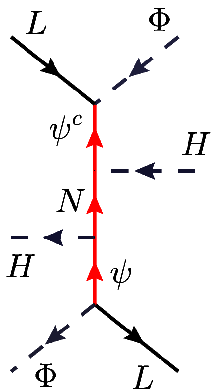
For completeness, we now discuss a model with scalar DM. Here we introduce a vector-like lepton doublet and a Weyl fermion singlet , denoted as
| (67) |
with all fields being left-handed. In addition, a complex scalar field which carries lepton number of is also introduced. The Lagrangian relevant to the neutrino-DM interaction is given by
| (68) | |||||
Here and are indices. Note that lepton number is conserved by this Lagrangian, as can be seen by assigning lepton numbers of for , for and zero for fields. This Lagrangian also preserves a discrete symmetry under which are odd, while all SM particles are even. This guarantees the stability of DM , which is assumed be the lightest of all -odd states. This model resembles the doublet-singlet fermionic DM model studied extensively in the literature (see e.g., Ref. Cohen et al. (2012)), but with the distinction that the singlet-doublet fermion sector serves as the mediator and not as the DM in the present case.
The mass matrix for the neutral leptons can be written down in the basis as
| (69) |
In contrast, the charged lepton is unmixed and has a mass given by . Direct searches for vector-like charged leptons at the LHC set limits of order 700 GeV on the mass of . In order to obtain large interactions, we choose the mass of the singlet fermion to be much smaller than the EWSB scale. To get simple analytic expressions, let us work in the limit where with the hierarchy . This will result in mixing given by the angle
| (70) |
The masses of and the heavier fields are given by
| (71) |
Now, the oblique electroweak precision parameter requires the mass-splittings between the two members of a leptonic doublet to be , which translates into a limit of , for GeV. We shall impose this condition in estimating the interaction strength.
The diagram shown in Fig. 7 will induce large interactions of the form
| (72) |
with an amplitude given by
| (73) |
Since the Yukawa couplings are only loosely constrained, and since the singlet fermion mass can be as low as a 100 MeV or so, the effective coupling can be quite large. Note that the effective coupling is suppressed by a factor of .
Finally, the case of vector DM is more challenging to UV-complete because the mediator must be charged under a gauge symmetry in order to couple to a vector field. We leave a detailed exploration of such models for future work.
6 Conclusions
We have presented a general framework to systematically study neutrino-DM interactions, both in the EFT approach and in UV-complete models. Starting from a low-energy DM-LEFT description and its gauge-invariant embedding in DM-SMEFT, we identified the leading non-derivative operator structures that couple neutrinos to fermionic, scalar, and vector DM candidates. We then classified the renormalizable tree-level UV completions of the relevant DM-SMEFT operators up to dimension-8 by enumerating the distinct diagram topologies and corresponding mediator particle quantum numbers, thereby providing a clear connection between the effective interactions and minimal UV field-content.
Using this EFT to UV framework, we constructed a few benchmark model realizations that can yield sizable neutrino-DM interactions, while avoiding potentially problematic charged-lepton interactions at the leading order, as well as the neutrino mass constraints. In particular, the inert-doublet scotogenic realization of a pseudo-Dirac DM with a light CP-even neutral scalar mediator illustrates how neutrino-dominated DM phenomenology can arise in this model and how a combination of the existing cosmology, flavor, electroweak precision, collider, and direct detection constraints carve out viable regions of parameter space with clear targets for future searches. In this model, we find that an effective neutrino-DM coupling as large as is allowed.
We also provided alternative model realizations for Majorana DM based on the type-II seesaw and inverse seesaw frameworks. The type-II version can give sizable neutrino-DM effective interactions as large as , while the inverse-seesaw version can give effective couplings comparable to . For completeness, we also discussed a simple model with scalar DM, where the effective neutrino-DM coupling can be much larger than . Given the large number of possible UV-completions of the effective operators listed here, we hope the model-building community can follow up with other interesting model realizations for large neutrino-DM interactions, thus shedding more light on the plausible connection between two of the least understood sectors in fundamental physics.
Acknowledgements.
We wish to acknowledge the Center for Theoretical Underground Physics and Related Areas (CETUP*) and the Institute for Underground Science at SURF for hospitality and for providing a stimulating environment during the 2025 Summer Workshop (Neutrino Weeks), where this work was initiated. K.S.B. and B.D. also thank the organizers of WHEPP 2025 at IIT, Hyderabad for local hospitality, where a part of this work was done. B.D. thanks Doojin Kim, Deepak Sathyan, Kuver Sinha and Yongchao Zhang for discussions on neutrino-DM interactions. A.T. thanks Julian Heeck for discussions on various topologies. The work of K.S.B. is supported by the US Department of Energy under grant number DE-SC0016013. The work of B.D. was partly supported by the US Department of Energy under grant No. DE-SC0017987 and by a Humboldt Fellowship from the Alexander von Humboldt Foundation. The work of A.T. is supported in part by the US Department of Energy grant DE-SC0010143.References
- [1] (2017) A search for doubly-charged Higgs boson production in three and four lepton final states at . Technical report Technical Report CMS-PAS-HIG-16-036. Cited by: 2nd item.
- Search for doubly charged Higgs boson production in multi-lepton final states with the ATLAS detector using proton–proton collisions at . Eur. Phys. J. C 78 (3), pp. 199. External Links: 1710.09748, Document Cited by: 2nd item.
- Search for anomalous production of prompt same-sign lepton pairs and pair-produced doubly charged Higgs bosons with TeV collisions using the ATLAS detector. JHEP 03, pp. 041. External Links: 1412.0237, Document Cited by: 2nd item.
- Search for electroweak production of charginos and sleptons decaying into final states with two leptons and missing transverse momentum in TeV collisions using the ATLAS detector. Eur. Phys. J. C 80 (2), pp. 123. External Links: 1908.08215, Document Cited by: §4.
- Search for doubly and singly charged Higgs bosons decaying into vector bosons in multi-lepton final states with the ATLAS detector using proton-proton collisions at = 13 TeV. JHEP 06, pp. 146. External Links: 2101.11961, Document Cited by: 1st item.
- Search for doubly charged Higgs boson production in multi-lepton final states using 139 fb-1 of proton–proton collisions at = 13 TeV with the ATLAS detector. Eur. Phys. J. C 83 (7), pp. 605. External Links: 2211.07505, Document Cited by: 2nd item.
- Search for electroweak production of supersymmetric particles in final states with two -leptons in = 13 TeV pp collisions with the ATLAS detector. JHEP 05, pp. 150. External Links: 2402.00603, Document Cited by: §4.
- First Dark Matter Search Results from the LUX-ZEPLIN (LZ) Experiment. Phys. Rev. Lett. 131 (4), pp. 041002. External Links: 2207.03764, Document Cited by: §4.4.
- Search for lepton-flavor-violating tau-lepton decays to at Belle. JHEP 10, pp. 19. External Links: 2103.12994, Document Cited by: §4.2.
- Determination of the number of light neutrino species from single photon production at LEP. Phys. Lett. B 431, pp. 199–208. External Links: Document Cited by: §5.
- Single photon and multiphoton events with missing energy in collisions at LEP. Phys. Lett. B 587, pp. 16–32. External Links: hep-ex/0402002, Document Cited by: §5.
- First Direct-Detection Results on Sub-GeV Dark Matter Using the SENSEI Detector at SNOLAB. Phys. Rev. Lett. 134 (1), pp. 011804. External Links: 2312.13342, Document Cited by: §5.
- New limit on the decay with the MEG II experiment. Eur. Phys. J. C 85 (10), pp. 1177. Note: [Erratum: Eur.Phys.J.C 85, 1317 (2025)] External Links: 2504.15711, Document Cited by: §4.2.
- Probing Benchmark Models of Hidden-Sector Dark Matter with DAMIC-M. Phys. Rev. Lett. 135 (7), pp. 071002. External Links: 2503.14617, Document Cited by: §5.
- Planck 2018 results. VI. Cosmological parameters. Astron. Astrophys. 641, pp. A6. Note: [Erratum: Astron.Astrophys. 652, C4 (2021)] External Links: 1807.06209, Document Cited by: §1, §4.3.
- Search for Dark-Matter–Nucleon Interactions via Migdal Effect with DarkSide-50. Phys. Rev. Lett. 130 (10), pp. 101001. External Links: 2207.11967, Document Cited by: §4.4.
- Direct evidence for neutrino flavor transformation from neutral current interactions in the Sudbury Neutrino Observatory. Phys. Rev. Lett. 89, pp. 011301. External Links: nucl-ex/0204008, Document Cited by: §1.
- Mono-Higgs Signature in the Scotogenic Model with Majorana Dark Matter. Phys. Rev. D 101 (3), pp. 035038. External Links: 1811.00490, Document Cited by: §4.
- Note on tree level unitarity in the general two Higgs doublet model. Phys. Lett. B 490, pp. 119–124. External Links: hep-ph/0006035, Document Cited by: §4.
- Constraints on dark matter-neutrino scattering from the Milky-Way satellites and subhalo modeling for dark acoustic oscillations. JCAP 11, pp. 037. External Links: 2305.01913, Document Cited by: §1.
- WIMP Dark Matter Search Using a 3.1 Tonne-Year Exposure of the XENONnT Experiment. Phys. Rev. Lett. 135 (22), pp. 221003. External Links: 2502.18005, Document Cited by: §4.4.
- Dark matter decay to neutrinos. Phys. Rev. D 108 (12), pp. 123021. External Links: 2210.01303, Document Cited by: §3.2.
- Precision Higgs Probe of Type-II Seesaw. External Links: 2512.07532 Cited by: 1st item.
- Low-mass doubly charged Higgs bosons at the LHC. Phys. Rev. D 107 (1), pp. 015018. External Links: 2211.00632, Document Cited by: 1st item.
- Revisiting type-II see-saw: present limits and future prospects at LHC. JHEP 03, pp. 195. External Links: 2108.10952, Document Cited by: 1st item.
- Searches for Lepton Flavor Violation in the Decays and . Phys. Rev. Lett. 104, pp. 021802. External Links: 0908.2381, Document Cited by: §4.2.
- Non-Standard Interactions in Radiative Neutrino Mass Models. JHEP 03, pp. 006. External Links: 1907.09498, Document Cited by: §1, §4, §4.
- Classification of effective neutrino mass operators. Nucl. Phys. B 619, pp. 667–689. External Links: hep-ph/0106054, Document Cited by: §2.
- Improved naturalness with a heavy Higgs: An Alternative road to LHC physics. Phys. Rev. D 74, pp. 015007. External Links: hep-ph/0603188, Document Cited by: §4.
- Simplified Dark Matter Models for the Galactic Center Gamma-Ray Excess. Phys. Rev. D 89 (11), pp. 115022. External Links: 1404.0022, Document Cited by: §4.3, §4.3.
- Lepton-Number-Charged Scalars and Neutrino Beamstrahlung. Phys. Rev. D 97 (7), pp. 075030. External Links: 1802.00009, Document Cited by: §1.
- Particle dark matter: Evidence, candidates and constraints. Phys. Rept. 405, pp. 279–390. External Links: hep-ph/0404175, Document Cited by: §1.
- Neutrino Portals to Dark Matter. Eur. Phys. J. C 79 (7), pp. 555. External Links: 1903.00006, Document Cited by: §1.
- Dark Matter Search Results from 1.54 Tonne·Year Exposure of PandaX-4T. Phys. Rev. Lett. 134 (1), pp. 011805. External Links: 2408.00664, Document Cited by: §4.4.
- Constraining dark matter candidates from structure formation. Phys. Lett. B 518, pp. 8–14. External Links: astro-ph/0012504, Document Cited by: §1.
- Neutrinoless double beta decay versus other probes of heavy sterile neutrinos. JHEP 03, pp. 170. External Links: 1912.03058, Document Cited by: §5.2.
- Systematic study of the d=5 Weinberg operator at one-loop order. JHEP 07, pp. 153. External Links: 1204.5862, Document Cited by: §2.
- Extended analysis of neutrino-dark matter interactions with small-scale CMB experiments. Phys. Dark Univ. 42, pp. 101321. External Links: 2305.01383, Document Cited by: §1.
- Revisiting neutrino self-interaction constraints from and decays. Phys. Rev. D 101 (11), pp. 115001. External Links: 2003.05339, Document Cited by: §1.
- Effective Lagrangian Analysis of New Interactions and Flavor Conservation. Nucl. Phys. B 268, pp. 621–653. External Links: Document Cited by: §2.
- From the trees to the forest: a review of radiative neutrino mass models. Front. in Phys. 5, pp. 63. External Links: 1706.08524, Document Cited by: §2.
- A direct empirical proof of the existence of dark matter. Astrophys. J. Lett. 648, pp. L109–L113. External Links: astro-ph/0608407, Document Cited by: §1.
- Singlet-Doublet Dark Matter. Phys. Rev. D 85, pp. 075003. External Links: 1109.2604, Document Cited by: §5.3.
- [44] (2000-12) Combination procedure for the precise determination of Z boson parameters from results of the LEP experiments. External Links: hep-ex/0101027 Cited by: 1st item.
- Closing in on singly charged scalars. Phys. Rev. D 112 (5), pp. 055003. External Links: 2506.05258, Document Cited by: §4.
- Pattern of Symmetry Breaking with Two Higgs Doublets. Phys. Rev. D 18, pp. 2574. External Links: Document Cited by: §4, §4.
- New Constraints on Neutrino-Dark Matter Interactions: A Comprehensive Analysis. External Links: 2507.01000 Cited by: §1, §1, §4.5, §4.5.
- New laboratory constraints on neutrinophilic mediators. Phys. Lett. B 868, pp. 139765. External Links: 2407.12738, Document Cited by: §1.
- Neutrino Non-Standard Interactions: A Status Report. SciPost Phys. Proc. 2, pp. 001. External Links: 1907.00991, Document Cited by: §1.
- Reducing the and tensions with Dark Matter-neutrino interactions. Phys. Rev. D 97 (4), pp. 043513. External Links: 1710.02559, Document Cited by: §1.
- First results from KamLAND: Evidence for reactor anti-neutrino disappearance. Phys. Rev. Lett. 90, pp. 021802. External Links: hep-ex/0212021, Document Cited by: §1.
- Exploring dark matter microphysics with galaxy surveys. JCAP 09, pp. 034. External Links: 1505.06735, Document Cited by: §1.
- General approach to neutrino mass mechanisms with sterile neutrinos. Phys. Rev. D 109 (7), pp. 073003. External Links: 2310.15379, Document Cited by: §4.1.
- Neutrino oscillations and Non-Standard Interactions. Front. in Phys. 6, pp. 10. External Links: 1710.09360, Document Cited by: §1.
- Neutrino Masses and the CERN LHC: Testing Type II Seesaw. Phys. Rev. D 78, pp. 015018. External Links: 0805.3536, Document Cited by: 1st item.
- GroupMath: A Mathematica package for group theory calculations. Comput. Phys. Commun. 267, pp. 108085. External Links: 2011.01764, Document Cited by: §3.
- Radiative Correction from Secret Neutrino Interactions and Implications for Neutrino-Scattering Experiments. External Links: 2510.15023 Cited by: §1.
- Evidence for oscillation of atmospheric neutrinos. Phys. Rev. Lett. 81, pp. 1562–1567. External Links: hep-ex/9807003, Document Cited by: §1.
- Exploding operators for Majorana neutrino masses and beyond. JHEP 01, pp. 074. External Links: 2009.13537, Document Cited by: §3.
- Large gauge invariant non-standard neutrino interactions. Phys. Rev. D 79, pp. 013007. External Links: 0809.3451, Document Cited by: §1.
- Neutrino-dark sector equilibration and primordial element abundances. Phys. Rev. D 111 (4), pp. 043526. External Links: 2402.10264, Document Cited by: §1.
- Cosmic abundances of stable particles: Improved analysis. Nucl. Phys. B 360, pp. 145–179. External Links: Document Cited by: §4.3.
- Dimension-Six Terms in the Standard Model Lagrangian. JHEP 10, pp. 085. External Links: 1008.4884, Document Cited by: §2.
- Freeze-In Production of FIMP Dark Matter. JHEP 03, pp. 080. External Links: 0911.1120, Document Cited by: footnote 6.
- [65] Opening up baryon-number-violating operators. Note: https://uva.theopenscholar.com/heeck/BNVAccessed: 2025-01-01 External Links: Document Cited by: §3.
- Light neutrinophilic dark matter from a scotogenic model. Phys. Lett. B 845, pp. 138167. External Links: 2307.15760, Document Cited by: §4.
- Dark matter direct detection of a fermionic singlet at one loop. Eur. Phys. J. C 78 (6), pp. 471. Note: [Erratum: None 82, 53 (2022)] External Links: 1803.05660, Document Cited by: §4.4.
- Constraining neutrino-DM interactions with Milky Way dwarf spheroidals and supernova neutrinos. Phys. Rev. D 110 (2), pp. 023004. External Links: 2402.08718, Document Cited by: §1.
- Hints of dark matter-neutrino interactions in Lyman- data. Phys. Rev. D 105 (10), pp. 103504. External Links: 2110.04024, Document Cited by: §1.
- IGraph/M: graph theory and network analysis for Mathematica. Journal of Open Source Software 8 (81), pp. 4899. External Links: ISSN 2475-9066, Link, Document Cited by: §3.
- Dirac dark matter with a charged mediator: a comprehensive one-loop analysis of the direct detection phenomenology. JCAP 05, pp. 047. External Links: 1503.03382, Document Cited by: §4.4.
- Direct Detection of Fermion Dark Matter in the Radiative Seesaw Model. Phys. Rev. D 93 (3), pp. 035012. External Links: 1601.01163, Document Cited by: §4.4, §4.4, footnote 5.
- Low-Energy Effective Field Theory below the Electroweak Scale: Operators and Matching. JHEP 03, pp. 016. Note: [Erratum: JHEP 12, 043 (2023)] External Links: 1709.04486, Document Cited by: §2.
- Mass bounds of the lightest CP even Higgs boson in the two Higgs doublet model. Phys. Lett. B 471, pp. 182–190. External Links: hep-ph/9903289, Document Cited by: §4.
- Bounds on the mass of doubly-charged Higgs bosons in the same-sign diboson decay scenario. Phys. Rev. D 90 (11), pp. 115018. External Links: 1407.6547, Document Cited by: 1st item.
- Radiative corrections to electroweak parameters in the Higgs triplet model and implication with the recent Higgs boson searches. Phys. Rev. D 85, pp. 115009. External Links: 1201.6287, Document Cited by: §5.1.
- Vacuum Stability Conditions From Copositivity Criteria. Eur. Phys. J. C 72, pp. 2093. External Links: 1205.3781, Document Cited by: §4.
- Right-Handed Neutrinos at CERN LHC and the Mechanism of Neutrino Mass Generation. Phys. Rev. D 76, pp. 073005. External Links: 0705.3221, Document Cited by: §4.1.
- Feyn Arts: Computer Algebraic Generation of Feynman Graphs and Amplitudes. Comput. Phys. Commun. 60, pp. 165–180. External Links: Document Cited by: §3.
- General formulae for f(1) — f(2) gamma. Eur. Phys. J. C 29, pp. 191–195. External Links: hep-ph/0302221, Document Cited by: §4.2.
- Proton Lifetime and Fermion Masses in an SO(10) Model. Nucl. Phys. B 181, pp. 287–300. External Links: Document Cited by: §5.1.
- Verifiable radiative seesaw mechanism of neutrino mass and dark matter. Phys. Rev. D 73, pp. 077301. External Links: hep-ph/0601225, Document Cited by: §4.1, §4.
- Neutrino Mass Problem and Gauge Hierarchy. Phys. Lett. B 94, pp. 61–64. External Links: Document Cited by: §5.1.
- Toward deconstructing the simplest seesaw mechanism. Phys. Rev. D 105 (9), pp. 095020. External Links: 2203.06362, Document Cited by: 1st item.
- Cosmological bounds on dark matter-neutrino interactions. Phys. Rev. D 74, pp. 043517. External Links: astro-ph/0606190, Document Cited by: §1.
- Relic neutrino decoupling including flavor oscillations. Nucl. Phys. B 729, pp. 221–234. External Links: hep-ph/0506164, Document Cited by: §1.
- Type II Seesaw at LHC: The Roadmap. Phys. Rev. D 85, pp. 055018. External Links: 1108.4416, Document Cited by: 1st item.
- Neutrino Mass and Baryon Number Nonconservation in Superstring Models. Phys. Rev. D 34, pp. 1642. External Links: Document Cited by: §5.2.
- Neutrino Masses and Mixings in Gauge Models with Spontaneous Parity Violation. Phys. Rev. D 23, pp. 165. External Links: Document Cited by: §5.1.
- Review of particle physics. Phys. Rev. D 110 (3), pp. 030001. External Links: Document Cited by: §4.4, §4, §5.1.
- Novel bounds on neutrino portal dark matter from leptonic meson decays. External Links: 2511.08102 Cited by: §1.
- Dark matter-neutrino interactions through the lens of their cosmological implications. Phys. Rev. D 97 (7), pp. 075039. External Links: 1711.05283, Document Cited by: §1.
- A New constraint on a strongly interacting Higgs sector. Phys. Rev. Lett. 65, pp. 964–967. External Links: Document Cited by: §4.
- Estimation of oblique electroweak corrections. Phys. Rev. D 46, pp. 381–409. External Links: Document Cited by: §4.
- Refined Bounds on MeV-scale Thermal Dark Sectors from BBN and the CMB. JCAP 01, pp. 004. External Links: 1910.01649, Document Cited by: §1.
- Precise WIMP Dark Matter Abundance and Standard Model Thermodynamics. JCAP 08, pp. 011. External Links: 2005.03544, Document Cited by: §4.3.
- Neutrino Masses in SU(2) x U(1) Theories. Phys. Rev. D 22, pp. 2227. External Links: Document Cited by: §5.1.
- MeV-mass dark matter and primordial nucleosynthesis. Phys. Rev. D 70, pp. 043526. External Links: astro-ph/0403417, Document Cited by: §1.
- Search for supersymmetry in final states with two oppositely charged same-flavor leptons and missing transverse momentum in proton-proton collisions at 13 TeV. JHEP 04, pp. 123. External Links: 2012.08600, Document Cited by: §4.
- Precise Relic WIMP Abundance and its Impact on Searches for Dark Matter Annihilation. Phys. Rev. D 86, pp. 023506. External Links: 1204.3622, Document Cited by: §4.3, §4.3.
- Radiative seesaw mechanism at weak scale. Phys. Rev. D 54, pp. 5693–5697. External Links: hep-ph/9603309, Document Cited by: §4.
- Search for direct pair production of supersymmetric partners of leptons in the final state with two hadronically decaying leptons and missing transverse momentum in proton-proton collisions at = 13 TeV. Phys. Rev. D 108 (1), pp. 012011. External Links: 2207.02254, Document Cited by: §4.
- Baryon and Lepton Nonconserving Processes. Phys. Rev. Lett. 43, pp. 1566–1570. External Links: Document Cited by: §2.
- Constraining Dark Matter-Neutrino Interactions using the CMB and Large-Scale Structure. JCAP 05, pp. 011. External Links: 1401.7597, Document Cited by: §1.