The species scale and the refined TCC bound in time-dependent backgrounds of string theory

As mentioned in the introduction, the TCC requires that for any expanding universe, the cosmological scale factor and the Hubble parameter over the time interval $[t_{i},t_{f}]$ must satisfy Eq. (1). While most discussions of the conjecture assume that the initial and final times, $t_{i}$ and $t_{f}$, are distinct, here we explore the special case where the initial and final times coincide, $t_{i}=t_{f}=t$,

$\displaystyle l_{P}<\frac{1}{H(t)},$

(8)

which asserts that the Hubble horizon must always be greater than the Planck length at all times.

The Hubble parameter in the de-Sitter spacetime is constant, imposing specific constraints on its value,

$\displaystyle H<\frac{1}{l_{P}},$

(9)

It is not surprising that the cosmological constant should not be too large, as the structure formation and the anthropic principle impose constraints on its value PhysRevLett.59.2607. Although Eq. (9) is, in some sense, trivial, reflecting the requirement that the energy scales remain below the Planck scale, it offers a more attractive and fundamental perspective. It also opens up scenarios in which dark energy can be analyzed. In particular, we will test it in the context of the refined TCC, which provides more nontrivial constraints on the dark energy.

Let us examine the refined TCC and explore how it constrains the Hubble constant. From the refined TCC (5), for $t_{i}=t_{f}$, we conclude that :

$\displaystyle l_{P}g_{s}(t)^{-\frac{2}{D-2}}<\frac{1}{H(t)}.$

(10)

For the de-Sitter spacetime with a constant Hubble parameter $H$, the following condition holds for all times:

$\displaystyle H<\frac{g_{s}(t)^{\frac{2}{D-2}}}{l_{P}}.$

(11)

The cosmological constant $\Lambda$, and the Hubble parameter $H$, are related by $H^{2}\sim\Lambda$. Therefore, the refined $TCC$ put an upper bound on the cosmological constant.

Equation (11) may explain "why the cosmological constant is so small compared to the Planck energy scale, $M_{P}^{2}$." The answer may lie in the fact that we live in an approximately free limit of string theory, where string interactions are not too large. However, it cannot solve the hierarchy of scales, as the species scales cannot be smaller than the energy scales, smaller than the TeV scale, where the standard model of particle physics, as an effective field theory give an accurate description of nature.

As mentioned in the introduction, the singularity theorems imply that general relativity, even at the classical level, is incomplete. Addressing this issue requires a deeper theory. A true quantum theory of gravity should provide a resolution to this problem. Two possible approaches to reformulating the answer are as follows:

• •

  Negative perspective: Resolving the issue by dissolving the problem, i.e., reinterpreting or reframing the singularities as artifacts of an incomplete framework rather than fundamental physical realities.

In such scenarios, which are the most plausible within a final quantum theory of gravity, the true degrees of freedom are not geometric, as in Riemannian geometry. Instead, singularities emerge as large-scale features of an emergent metric. In this framework, discussing lengths around the Planck scale becomes meaningless, and the problem of singularities naturally dissolves within this picture.

• •

  Positive perspective: Addressing the problem directly by finding solutions within the framework of an effective field theory for gravity, where singularities are resolved by some higher derivative or matter terms.

From this perspective, although the theory of quantum gravity might not be formulated using geometric ingredients, any UV completion of general relativity should admit an effective action expressed in geometric terms. We require that this action prohibit any singular metric as a solution to its equations of motion.

String theory’s dualities, such as $AdS/CFT$, $T$-duality, and mirror symmetry, suggest that duality-invariant quantities are not inherently geometric. This points to a deeper, yet-to-be-discovered mathematical structure underlying all currently known concepts, which represents the true mathematical foundation of string theory. In certain extreme limits of the moduli space parameters, this structure reduces to the familiar string theories. From this perspective, string theory may align with the negative approach, dissolving the problem of singularities by rendering them artifacts of an emergent description.

Nevertheless, in certain extreme limits of the parameter space, examples of string theory can still be formulated in terms of geometric concepts and effective actions. This holds for all known examples of string theory, at least to some order in the string length $l_{s}$ and the string coupling constant $g_{s}$. By turning off all non-geometric fields, such as the Kalb-Ramond field and others, and assuming a constant dilaton field $\phi$, the tree-level effective action takes a higher derivative expansion in terms of $l_{s}$ as follows

$\displaystyle S\sim\int d^{d+1}x\sqrt{-g}e^{-2\phi}\Big(\mathcal{R}+\lambda l_{s}^{2}\mathcal{R}_{\mu\nu\rho\sigma}\mathcal{R}^{\mu\nu\rho\sigma}+...\Big),$

(12)

where $\lambda$ is a different real number for different string theories. From this perspective, we may expect that string theory resolves at least some of the most challenging singularities, such as the big-bang or those arising in black holes.¹¹1String theory may permit certain types of singularities, such as orbifold singularities, which are well understood and controllable. However, in this paper, we focus exclusively on the big bang singularity and assume that string theory resolves it. This view aligns with the positive perspective in the perspectives. For the remainder of this paper, we adopt this view, and whenever we refer to string theory resolving a singularity, it should be understood in light of this framework.

Adopting this interpretation of resolving the big bang singularity, the effective actions of string theories, to all orders in $\alpha^{\prime}$ and $g_{s}$, share a similar nature as (12), with the inclusion of additional matter fields. Based on the TCC, all expanding universes derived from this action must satisfy the TCC bound. Let us examine whether power-law expansions, $a(t)\sim t^{\alpha}$, are compatible with the TCC and the refined TCC or not. The TCC-bound Eq. (8) becomes particularly interesting, as the Hubble horizon grows linearly with time

$\displaystyle\frac{1}{H}\sim t,$

(13)

and Eq. (8) then leads to the following inequality

$\displaystyle l_{P}<t,$

(14)

near the big bang singularity at $t\sim 0$, the length of the Hubble horizon can become smaller than the Planck length, violating the bound Eq. (8). Indeed, the relation Eq. (8) supports the no-singularity conjecture, suggesting that the big bang singularity should be resolved by some mechanism, possibly through the inclusion of higher-curvature and loop corrections in string theory to satisfy the bound Eq. (8).

Let us focus on the curvature invariants. The Kretschmann invariant for the $FRW$-metric is given by

$\displaystyle K=R_{\mu\nu\rho\sigma}R^{\mu\nu\rho\sigma}=12\Big((H^{\prime}+H^{2})^{2}+(\frac{k}{a^{2}}+H^{2})^{2}\Big),$

(15)

the bound Eq.(8) puts an upper bound on the Hubble parameter. Using the time reversal version of the TCC Eq.(2), we conclude that $a_{f}$ never reaches zero in a contracting universe by starting from initial values, $H_{i}$ and $a_{i}$. Therefore, $a_{f}$ is bounded from below. It is natural to assume that $H^{\prime}$ is also bounded; thus, the Kretschmann invariant is always finite and cannot diverge.

Without assuming the finiteness of $H^{\prime}$, one can give a simple argument for the no-singularity conjecture. For example, the expansion scalar $\theta$, has a clean geometrical meaning which quantifies the fractional rate of change of volume (area) $\frac{1}{\delta V}\frac{d\delta V}{d\tau}$($\frac{1}{\delta A}\frac{d\delta A}{d\tau}$) for time-like (null-like) geodesics. The Raychaudhuri’s equation for a congruence of time-like geodesics is given by Poisson:2009pwt,

$\displaystyle\frac{d\theta}{d\tau}=-\frac{1}{3}\theta^{2}-\sigma^{\alpha\beta}\sigma_{\alpha\beta}+\omega^{\alpha\beta}\omega_{\alpha\beta}-R^{\alpha\beta}u_{\alpha}u_{\beta},$

(16)

is the fundamental equation in exploring the singularity theorems and shows the importance of $\theta$ in analyzing singularities. Let us consider a congruence of comoving world lines in an expanding universe with the following metric in $D=3+1$ spacetime

$\displaystyle ds^{2}=-dt^{2}+a^{2}(t)d\vec{x}^{2},$

(17)

and the expansion scalar for the tangent vectors $u_{\alpha}=-\partial_{\alpha}t$, is given by

$\displaystyle\theta=\frac{1}{a^{3}}\frac{da^{3}}{dt}=3H,$

(18)

and when the TCC satisfies, Eq.(9) implies that $\frac{1}{3}|\theta|<\frac{1}{l_{P}}$. Therefore, for such spacetimes, a caustic point ($|\theta|=\infty$) cannot form.

The refined TCC (5) provides a different constraint and does not exclude the singularity in the same way as the TCC. The constraint derived from the refined TCC for power-law expansions is given by

$\displaystyle\frac{l_{P}}{t}<g_{s}(t)^{\frac{2}{D-2}},$

(19)

This implies that the string coupling at any time $t$ cannot be smaller than the bound above. It results in the unbounded growth of the string coupling at early times. Assuming that the string coupling cannot diverge, this behavior is also incompatible with power-law singularities.

It appears that the refined TCC imposes a stronger constraint at late times $t\to\infty$ compared to the TCC. For instance, it places a more restrictive bound on the cosmological constant (11). However, at early times $t\to 0$, the TCC is more effective in excluding any big bang singularity at $t=0$. We can summarize the implications of the TCC and refined TCC for the cosmological constant $\Lambda$, and the big bang singularity as follows:

	Bound on the cosmological constant $\Lambda$ for de-Sitter Space time	The existence of singularity
The TCC	$\Lambda<\frac{1}{l_{P}^{2}}$	incompatible
The refined TCC	$\Lambda<\frac{g_{s}(t)^{\frac{4}{D-2}}}{l_{P}^{2}}$	incompatible

In the following section, we explore the pre-big bang and string gas cosmology scenarios to provide further evidence for the no-singularity conjecture and to distinguish between the TCC and the refined TCC.

In all 10-dimensional superstring theories, there exists a dilaton. Thus, it provides an interesting framework to test the refined 10-dimensional TCC. The string action in the supergravity approximation is given by

$\displaystyle S$

$\displaystyle=$

$\displaystyle\int d^{10}x\sqrt{-G}\frac{1}{2\kappa_{10}^{2}}e^{-2\phi}\Big(R+4(\partial_{\mu}\phi)^{2}\Big).$

(20)

where $\kappa_{10}^{2}=8\pi G_{10}$. By going to the Einstein frame with the proper Weyl transformation $(g^{E}_{\mu\nu}=e^{-\frac{1}{2}\phi}g^{S}_{\mu\nu})$, the Friedmann equations take the following form in ten dimensions

	$\displaystyle 9H^{2}$	$\displaystyle=$	$\displaystyle\pi G_{10}\dot{\hat{\phi}}^{2},$		(21)
	$\displaystyle\dot{H}$	$\displaystyle=$	$\displaystyle-\pi G_{10}\dot{\hat{\phi}}^{2},$		(22)

where we have assumed the flat FRW metric, expressed as

$\displaystyle ds^{2}=-dt^{2}+a^{2}(t)d\vec{x}^{2},\penalty 10000\ \penalty 10000\ \penalty 10000\ \phi=\phi(t)$

(23)

and normalized $\phi$ into it’s canonical form through the rescaling $\hat{\phi}=\frac{1}{\sqrt{2}\kappa_{10}}\phi$. The solutions of the above equations are as follows

$\displaystyle H=\frac{1}{9t},\penalty 10000\ \penalty 10000\ \penalty 10000\ \phi(t)=-\frac{4}{3}Ln(\frac{t}{t_{0}}),$

(24)

where $t_{0}$ is an undetermined constant. The equation of motion for $\hat{\phi}$ is trivially satisfied by the solutions. To be compatible with supergravity approximation and the weak coupling limit, we require $g_{s}=e^{\phi}<1$. Consequently, the above solutions should be considered at late times, $t\gg t_{0}$. Since the string length is related to the Planck length by $l_{P}=l_{s}e^{\frac{\phi}{4}}$, the refined TCC, expressed in Planck units, takes the following form

$\displaystyle(\frac{t_{f}}{t_{i}})^{\frac{1}{9}}(\frac{t_{i}}{t_{0}})^{\frac{1}{3}}<9t_{f}.$

(25)

The above bound is clearly satisfied at late times. By choosing $t_{0}$ sufficiently small, we can also test the relation at relatively early times. The string coupling constant is

$\displaystyle g_{s}=(\frac{t_{0}}{t})^{\frac{4}{3}}$

(26)

Moreover, if we choose the initial time $t_{i}$ to be a few orders of magnitude larger than $t_{0}$, the loop expansion of string theory remains reliable even at early times, since the string coupling $g_{s}(t_{i})$ can be taken to be small. However, one must also ensure that the spacetime curvature remains under control: the curvature length scales, governed by $H$ and $\dot{H}$, must be larger than the string length. More precisely

$\displaystyle\frac{1}{H}>l_{s},\penalty 10000\ \penalty 10000\ \penalty 10000\ 9t>(\frac{t}{t_{0}})^{\frac{1}{3}}$

(27)

The above relation is satisfied only if

$\displaystyle t>\frac{1}{27\sqrt{t_{0}}},$

(28)

the optimal choice consistent with both Eqs. (26) and (27) is $t_{0}=\frac{1}{9}l_{p}$²²2We keep the Planck length explicit in order to compare $t_{0}$ with the Planck time.. This implies that, by taking $t_{0}$ to be of order the Planck time, one can safely trust the bounds (26) and (27) and test the refined TCC even at early times, provided the initial time $t_{i}$ is larger than $t_{0}$, as is always the case in standard cosmological scenarios. For this range of parameters, the refined TCC is satisfied even at early times.

To explore the refined TCC beyond the supergravity approximation in uncompactified string theories, we focus on O(16)$\times$O(16) string theory, which can be constructed by twisting $E_{8}\times E_{8}$ string theory Alvarez-Gaume; Dixon:1986iz, and is characterized by a positive vacuum energy coming from one-loop diagrams in the string frame. It is non-supersymmetric and therefore is not a superstring theory. However, due to the simplicity of its effective action, one can check the refined TCC straightforwardly. The effective action of the $O(16)\times O(16)$ string theory in string frame is as follows obied2018sitterspaceswampland:

$\displaystyle S$

$\displaystyle=$

$\displaystyle\int d^{10}x\sqrt{-G}\left[\frac{1}{2\kappa_{10}^{2}}e^{-2\phi}\Big(R+4(\partial_{\mu}\phi)^{2}\Big)-\Lambda\right].$

(29)

where $\kappa_{10}$ is $\kappa_{10}^{2}=8\pi G_{10}$. We consider a class of metrics in the string frame in such a way

$\displaystyle ds^{2}=g_{\mu\nu}dx^{\mu}dx^{\nu}+e^{2\rho(x)}\gamma_{ab}dy^{a}dy^{b},$

(30)

where $\mu$ and $\nu$ run over $\mu$,$\nu=0,1,...,D=d+1$, while $a$, $b$ are indices for $10-D$ compactified manifold. We consider $\rho(x)$ as the only Kahler modulus. For simplicity, in the following, we further assume that the Kähler modulus is also stabilized. Therefore, the $D$-dimensional action after compactification in the Einstein frame is given by

$\displaystyle S=\int d^{D}x\sqrt{-g}\Big(\frac{1}{2\kappa_{D}^{2}}R-\frac{1}{2}(\partial\hat{\phi})^{2}-\Lambda_{D}e^{\frac{D}{\sqrt{D-2}}\kappa\hat{\phi}}\Big)$

(31)

where $\hat{\phi}$ is defined by $\hat{\phi}=\frac{2}{\sqrt{D-2}}\frac{\phi}{\kappa_{D}}$, $\Lambda_{D}=\Lambda V_{10-D}$ and $\kappa_{10}^{2}=\kappa_{D}^{2}V_{10-D}$ where $V_{10-D}$ is the volume of the compact manifold in the string frame. The Friedmann equations are given by

	$\displaystyle(D-1)(D-2)H^{2}$	$\displaystyle=$	$\displaystyle 2\kappa_{D}^{2}(\frac{1}{2}\dot{\hat{\phi}}^{2}+V),$		(32)
	$\displaystyle(D-2)\dot{H}$	$\displaystyle=$	$\displaystyle-\kappa_{D}^{2}\dot{\hat{\phi}}^{2},$		(33)

and the equation of motion for $\hat{\phi}$ is as follows

$\displaystyle\ddot{\hat{\phi}}+(D-1)H\dot{\hat{\phi}}+\partial_{\hat{\phi}}V=0,$

(34)

where $V$ is given by $V=\Lambda_{D}e^{\frac{D}{\sqrt{D-2}}\kappa_{D}\hat{\phi}}$. The most general solution of the above equations is as follows Russo_2004:

	$\displaystyle\hat{\phi}=\frac{1}{\kappa_{D}}\sqrt{\frac{D-2}{D-1}}(U(\tau)-V(\tau)),$		(35)
	$\displaystyle a(\tau)^{D-1}=e^{U+V},$		(36)

where $U$ and $V$ and $\tau$ are defined by

	$\displaystyle U(\tau)$	$\displaystyle=$	$\displaystyle\frac{2\sqrt{D-1}}{D+2\sqrt{D-1}}Log\Big(sin(\beta(\tau-\tau_{0}))\Big),$		(37)
	$\displaystyle V(\tau)$	$\displaystyle=$	$\displaystyle-\frac{2\sqrt{D-1}}{D-2\sqrt{D-1}}Log\Big(Cos(\beta(\tau-\tau_{0}))\Big),$		(38)
	$\displaystyle\frac{d\tau}{dt}$	$\displaystyle=$	$\displaystyle\kappa_{D}\sqrt{\frac{D-1}{2(D-2)}\Lambda_{D}}\penalty 10000\ e^{\frac{D}{2\sqrt{D-1}}(U-V)}$		(39)
	$\displaystyle\beta$	$\displaystyle\equiv$	$\displaystyle\frac{D-2}{2\sqrt{D-1}}$

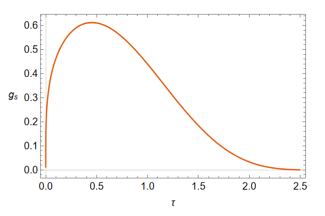
In the following, we set $\tau_{0}=0$. The range of $\tau$ is bounded as $\tau\in(0,\frac{\pi\sqrt{D-1}}{D-2})$, which corresponds to $t\in(0,\infty)$. The above solution describes an expanding universe with a singularity at $t=0$. To be consistent with perturbation theory, we consider the solution in the weak coupling limit $g_{s}=e^{\phi}\ll 1$, and require the radius of curvature of spacetime to be much larger than the string length, $H\ll\frac{1}{l_{s}}$. The dilaton field in terms of $\hat{\phi}$ is given by $\phi=\frac{\sqrt{D-2}}{2}\kappa\hat{\phi}$. Consequently, the string coupling is expressed as

$\displaystyle g_{s}=\left(sin(\beta\tau)\right)^{\alpha_{+}}\left(Cos(\beta\tau)\right)^{\alpha_{-}},$

(40)

where $\alpha_{\pm}$ are defined by $\alpha_{\pm}=\frac{D-2}{D\pm 2\sqrt{D-1}}$, which are positive for $D>3$. Therefore, the string coupling is weak at both asymptotic limits, $\tau=0$ and $\tau=\frac{\pi\sqrt{D-1}}{D-2}$ for $D>3$ as is shown in Fig. 1

We must also consider the weak gravity limit $H\ll\frac{1}{l_{s}}$. These conditions will simultaneously be satisfied in late times. The Hubble parameter is given by

$\displaystyle H=\sqrt{\frac{\kappa_{D}^{2}\Lambda_{D}}{2(D-1)(D-2)}}\Big(\alpha_{+}cot(\beta\tau)+\alpha_{-}tan(\beta\tau)\Big)(Sin(\beta\tau))^{\frac{D}{D+2\sqrt{D-1}}}(Cos(\beta\tau))^{\frac{D}{D-2\sqrt{D-1}}}.$

At late times, the curvature goes to zero. Let us directly test the refined TCC for the above solution. The $\kappa^{2}\Lambda_{D}$ does not depend on the volume of the compact manifold, and indeed we have $\kappa_{D}^{2}\Lambda_{D}=\kappa_{10}^{2}\Lambda$. $\kappa^{2}_{10}=8\pi l_{p,10}^{8}$ and as as noted in Alvarez-Gaume, $\Lambda$ is determined by the $l_{s}$ in string frame. In the ten-dimensional Planck length units, we take $\kappa^{2}\Lambda=12$, which means that the ten-dimensional Planck length and the string length in the string frame are of the same order. In the weak coupling limit, $e^{\phi}<1$, the species scale is the string length (in the Einstein frame), which in the ten-dimensional Planck length is $l_{s}=e^{-\frac{\phi}{4}}$. Furthermore, we allow an $O(1)$ constant $K$ in the refined TCC inequality as follows

$\displaystyle\frac{a(\tau_{f})}{a(\tau_{i})}e^{-\frac{\phi(\tau_{i})}{4}}<K\frac{1}{H_{f}}$

(42)

As is shown in Fig. 2, the refined TCC is satisfied for $D=4$.

It can be shown that the refined TCC is also satisfied in $D>4$.

In the following, we examine the refined TCC for type II superstrings, including different fluxes. The type II effective actions take the following general forms³³3We have used the notations of Hertzberg_2007. becker2006string; Hertzberg_2007

$\displaystyle S$

$\displaystyle=$

$\displaystyle\frac{1}{2\kappa_{10}^{2}}\int d^{10}x\sqrt{-g}e^{-2\phi}\left(R+4(\partial_{\mu}\phi)^{2}-\frac{1}{2}|H_{3}|^{2}-\frac{1}{2}e^{2\phi}\sum_{p}|F_{p}|^{2}\right)$

where we have rescaled the self-dual five form in IIB as $\tilde{F}_{5}\to\sqrt{2}\tilde{F}_{5}$. Once again, we assume that the Kahler moduli $\rho(x)$ is stabilized in the metric (30) and the dilaton is the only scalar field in the theory. Furthermore, we assumed that the internal manifold is Ricci flat. Therefore, compactifying down to D dimensions leads to the following effective action

$\displaystyle S=\int d^{D}x\sqrt{-g^{(D)}}\left(\frac{R}{2\kappa^{2}}-\frac{1}{2}(\partial\hat{\tau})^{2}-V_{H_{3}}e^{\frac{2}{\sqrt{D-2}}k\hat{\tau}}-\sum_{p}V_{F_{p}}e^{\frac{D}{\sqrt{D-2}}\kappa\hat{\tau}}\right)$

(44)

where we have defined $\tau\equiv e^{-\phi}$ and rescaled $\tau$ as $\hat{\tau}=\frac{2}{\sqrt{D-2}}\frac{\phi}{\kappa}$ to transform $\tau$ into the canonical form. $V_{H_{3}}$ and $V_{F_{p}}$ are positive coefficients which are related to the flux of $H_{3}$ and $F_{p}$. In the type IIA, $F_{p}$ are allowed when $p$ is even, and for the type IIB, they are odd. Let us focus on the Kalb-Ramond field strength $H_{3}$ and the Ramond-Ramond field strengths separately.

• •

  The Kalb-Ramond flux $H_{3}$

The solution takes an easy form as follows

$\displaystyle H=\frac{1}{t},\penalty 10000\ \penalty 10000\ \penalty 10000\ \penalty 10000\ \hat{\tau}=-\frac{\sqrt{D-2}}{\kappa}Log(\frac{t}{t_{0}}),$

(45)

where $t_{0}$ is equal to $t_{0}^{2}=\frac{(D-2)^{2}}{2V_{H_{3}}\kappa^{2}}$. From the action (3.3), we find that $\kappa_{D}^{2}V_{H_{3}}=\frac{\int H_{3}^{2}}{4V_{10-D}}$ where the integration in over the compact manifold. To be compatible with $\alpha^{\prime}$ expansion of string theory, we have to have $\frac{\int H^{2}_{3}}{V_{10-D}}>\frac{1}{l_{s}^{2}}$ where $l_{s}$ is the string length in the string frame. Therefore, we always have

$\displaystyle t_{0}>l_{s}.$

(46)

in the string frame.

The dilaton field is then $\phi=\frac{\sqrt{D-2}}{2}\kappa\hat{\tau}=-\frac{D-2}{2}Log(\frac{t}{t_{0}})$. The weak coupling limit corresponds to $t\gg t_{0}$. In the ten-dimensional Planck length units, the string length is given by $l_{s}=e^{-\frac{\phi}{4}}$. In $D=4$, the refined TCC takes the following form

$\displaystyle\frac{t_{f}}{t_{i}}(\frac{t_{i}}{t_{0}})^{\frac{1}{4}}<\frac{K}{H_{f}}=Kt_{f},$

(47)

which is equivalent to

$\displaystyle(\frac{1}{t_{0}t_{i}^{3}})^{\frac{1}{4}}<K,$

(48)

The relation (46) and weak coupling limit show that $t_{i}>t_{0}>1$ in the ten-dimensional Planck units, the above relation is satisfied for all $O(1)$ constant number $K>1$.

• •

  The RR fluxes $F_{p}$

For the RR-fluxes, as the exponent of the exponential is the same as $O(16)\times O(16)$ string theory, the refined TCC is also true for this sector. However, for having non-zero coefficients for $V_{F_{p}}$, $D$ should be smaller than eight, $D\leq 8$.

In the string frame, the bosonic part of the type I superstring is as followsbecker2006string

$\displaystyle S$

$\displaystyle=$

$\displaystyle\frac{1}{2\kappa_{10}^{2}}\int d^{10}x\sqrt{-g}\left[e^{-2\phi}\Big(R+4(\partial_{\mu}\phi)^{2}\Big)-\frac{1}{2}|\tilde{F}_{3}|^{2}-\frac{\kappa_{10}^{2}}{g^{2}}e^{-\phi}tr(|F_{2}|^{2})\right]$

where $F_{2}=dA+A\wedge A$ is the Yang-Mills strength corresponding to the gauge field $A+A_{\mu}dx^{\mu}$ and $g^{2}$ is given in terms of string length in the string frame as $\frac{g^{2}}{4\pi}=(2\pi l_{s})^{6}$. The $\tilde{F}_{3}$ is given by

$\displaystyle\tilde{F}_{3}=dC_{2}+\frac{l_{s}^{2}}{4}\omega_{3}.$

(50)

where $l_{s}$ is the string length in the string frame. $\omega_{3}$ is defined by

$\displaystyle\omega_{3}=\omega_{L}-\omega_{YM},$

(51)

where

$\displaystyle\omega_{L}=tr(\omega d\omega+\frac{2}{3}\omega^{3}),$

(52)

and

$\displaystyle\omega_{YM}=tr(AdA+\frac{2}{3}A^{3}),$

(53)

where $\omega_{L}$ and $\omega_{YM}$ is the Lorentz and Yang-Mills Chern-Simons terms. We just focus on the potential coming from the Yang-Mills part in terms of the field $\hat{\tau}$ in the last section, in a similar compactification. The effective potential is given by

$\displaystyle V_{eff}=V_{F_{2}}e^{\frac{D+2}{2\sqrt{D-2}}\kappa\hat{\tau}},$

(54)

where $V_{F_{2}}$ is a positive coefficient related to the flux of the Yang-Mills field strength. The solution for the Friedmann equations (32), (32) and (34) are given by

$\displaystyle H=\frac{16}{(D+2)^{2}t},\penalty 10000\ \penalty 10000\ \penalty 10000\ \penalty 10000\ \hat{\tau}=-\frac{4\sqrt{D-2}}{(D+2)\kappa_{D}}Log(\frac{t}{t_{0}}),$

(55)

where $t_{0}$ is defined as

$\displaystyle t_{0}^{2}=\frac{8}{\kappa_{D}^{2}V_{F_{2}}}\frac{\Big(16(D-1)-(D+2)^{2}\Big)(D-1)}{(D+4)^{2}}.$

(56)

which is positive for $2<D<10$. From the action (3.4), we find that

$\displaystyle\kappa_{D}^{2}V_{F_{2}}=\frac{l_{p,10}^{8}}{(2\pi l_{s})^{6}}\frac{\int|F_{2}|^{2}}{V_{10-D}},$

(57)

and for consistency with $\alpha^{\prime}$ expansion in string theory, we have to have $\frac{\int|F_{2}|^{2}}{V_{10-D}}<\frac{1}{l_{s}^{4}}$ in the string frame. Therefor, $t_{0}$ needs to be greater than $l_{s}$ in the string frame at least one order of magnitude.

The solution of dilaton using the equation (55) is given by

$\displaystyle\phi=-\frac{D-2}{D+2}Log(\frac{t}{t_{0}}),$

(58)

and the string coupling is weak when $t\gg t_{0}$. The refined TCC takes the following form

$\displaystyle\frac{t_{f}^{\frac{16}{(D+2)^{2}}}}{t_{i}^{\frac{16}{(D+2)^{2}}}}(\frac{t_{i}}{t_{0}})^{\frac{D-2}{4(D+2)}}<K\frac{(D+2)^{2}t_{f}}{16},$

(59)

Since the weak coupling limit $e^{\phi}<1$ gives $t_{f}>t_{i}>t_{0}$, and the consistency of $\alpha^{\prime}$ expansion of string theory in the ten-dimensional Planck units also leads to $t_{0}>1$, the above relation is satisfied.

The bosonic part of the effective action of the massless states of heterotic strings takes the following form

$\displaystyle S$

$\displaystyle=$

$\displaystyle\frac{1}{2\kappa_{10}^{2}}\int d^{10}x\sqrt{-g}e^{-2\phi}\left[R+4(\partial_{\mu}\phi)^{2}-\frac{1}{2}|\tilde{H}_{3}|^{2}-\frac{\kappa_{10}^{2}}{30g^{2}}Tr(F^{2}_{2})\right]$

where $F_{2}$ is the Yang-Mills field strength for gauge groups $E_{8}\times E_{8}$ and $SO(32)$. The field strength $\tilde{H}_{3}$ is defined by

$\displaystyle\tilde{F}_{3}=dB_{2}+\frac{l_{s}^{2}}{4}\omega_{3}.$

(61)

which satisfies the relation

$$d\tilde{H}_{3}=\frac{l_{s}^{2}}{4}\left(\text{tr}\,R\wedge R-\frac{1}{30}\text{Tr}\,F\wedge F\right)$$

where $Tr$ is the trace in the adjoint representation. As we see, the effective potential $V_{eff}$ coming from the Yang-Mills is the same as the effective potential coming from $H_{3}$ in II theories. Therefore, the refined TCC is also satisfied for the corresponding solutions with the same reasoning.

For more general compactifications, suppose that the volume of the compact dimension in the string frame is $e^{(10-D)\rho}$, then $\hat{\rho}$ is the canonical scalar field in the Einstein frame, which is related to $\rho$ as $\kappa_{D}\hat{\rho}=\sqrt{10-D}\rho$. Let us define $\hat{\tau}$ as $\kappa_{D}\hat{\tau}\equiv\frac{2}{\sqrt{D-2}}(\phi-\frac{\sqrt{10-D}}{2}\kappa_{D}\hat{\rho})$, then the effective potential of the D-dimensional theory takes the following form obied2018sitterspaceswampland

$\displaystyle V_{eff}=V_{\mathcal{R}}e^{-\frac{2}{\sqrt{10-D}}\kappa_{D}\hat{\rho}+\frac{2}{\sqrt{D-2}}\kappa_{D}\hat{\tau}}+\Lambda e^{\sqrt{10-D}\kappa_{D}\hat{\rho}+\frac{D}{\sqrt{D-2}}\kappa_{D}\hat{\tau}},$

(66)

where $V_{\mathcal{R}}$ comes from the Ricci scalar part of the compact manifold. For simplicity, we assume that the compact manifold $\gamma_{ab}$ in Equation (30) is Ricci flat, hence $V_{\mathcal{R}}=0$. The Friedmann equations and the equations of motion for $\hat{\rho}$ and $\hat{\tau}$ for the ansatz (23) change as follows

	$\displaystyle(D-1)(D-2)H^{2}=2\kappa_{D}^{2}(\frac{1}{2}\dot{\hat{\rho}}^{2}+\frac{1}{2}\dot{\hat{\tau}}^{2}+V),$		(67)
	$\displaystyle(D-2)\dot{H}=-\kappa_{D}^{2}(\dot{\hat{\rho}}^{2}+\dot{\hat{\tau}}^{2}),$		(68)
	$\displaystyle\ddot{\hat{\rho}}+(D-1)H\dot{\hat{\rho}}+\partial_{\hat{\rho}}V_{eff}=0,$		(69)
	$\displaystyle\ddot{\hat{\tau}}+(D-1)H\dot{\hat{\tau}}+\partial_{\hat{\tau}}V_{eff}=0.$		(70)

The general solutions of these equations are discussed in Appendix 7. For $O(16)\times O(16)$ string theory, the solutions are given by

	$\displaystyle u(\tau)=-\frac{\alpha_{1}A+\alpha_{2}B}{2\beta}(\tau-\tau_{0})-\frac{1}{\beta}Log\left(Cosh(\frac{1}{2}C(\tau-\tau_{0}))\right)+\tilde{d}_{0},$		(71)
	$\displaystyle\hat{\rho}=A(\tau-\tau_{0})-\frac{\alpha_{1}}{2\kappa_{D}^{2}}\frac{D-2}{D-1}u+d_{1},$		(72)
	$\displaystyle\hat{\tau}=B(\tau-\tau_{0})-\frac{\alpha_{2}}{2\kappa_{D}^{2}}\frac{D-2}{D-1}u+d_{2}$		(73)

where $A,B,d_{1},d_{2},\tilde{d}_{0}$ are integration constants, while $C$ and $\beta$, for a potential of the form $V=V_{0}e^{\alpha_{1}\hat{\rho}+\alpha_{2}\hat{\tau}}$ are defined in terms of $A$ and $B$ as follows

$\displaystyle\beta=1-\frac{D-2}{D-1}\frac{\alpha_{1}^{2}+\alpha_{2}^{2}}{4\kappa_{D}^{2}},\penalty 10000\ \penalty 10000\ \penalty 10000\ C^{2}=4\kappa_{D}^{2}\frac{D-1}{D-2}(A^{2}+B^{2})-(\alpha_{1}B-\alpha_{2}A)^{2}.$

(74)

The time variable $\tau$ is related to physical time $t$ via $\frac{d\tau}{dt}=e^{-u}$, and the scale factor in terms of $u$ is given by $a^{D-1}=e^{u}$. For the following considerations, we set $\tau_{0}$ equal to zero, which implies $a(\tau_{0})=1$. For $O(16)\times O(16)$ string theory, $\beta$ is given by

$\displaystyle\beta$

$\displaystyle=$

$\displaystyle 1-\frac{3D-5}{D-1},$

(75)

which is always negative for $10\geq D\geq 3$. As noted in Appendix 7, having a solution requires $C^{2}$ to be positive. For $D=4$, $C^{2}$ is given by

$\displaystyle C^{2}=\kappa_{D}^{2}(-2A^{2}+8\sqrt{3}AB)$

(76)

Assuming $A,B>0$, this leads to the inequality $A<4\sqrt{3}B$. It is not obvious that we can find solutions that are consistent with the validity of the weak gravity and weak coupling expansions. However, one can find that for the following range of parameters, there exist solutions

$\displaystyle\frac{2}{\sqrt{3}}-1<x<\frac{1}{4\sqrt{3}},$

(77)

where $x$ is defined by $x=\frac{B}{A}$. Let us assume $x=0.15$ and $A\kappa_{D}=1$. Under these assumptions, the solution simplifies as follows:

$\displaystyle a(\tau)^{3}=e^{\frac{3(\sqrt{6}+0.3\sqrt{2})\tau}{8}}Cosh(\frac{1}{2}C\tau)^{\frac{3}{4}}$

(78)

where $C=0.28$. The solution shows a singularity at $\tau=-\infty$ which corresponds to $t=0$ in physical time. The string coupling $g_{s}$ is shown in Fig 3, which remains consistent with perturbation theory at late times.

The warp factor in Equation (30), given by $e^{2\rho}=e^{\sqrt{\frac{2}{3}}\kappa_{D}\hat{\rho}}$, shows a decompactified phase at late times, as illustrated in Fig. 4.

In the ten-dimensional Planck length units, the refined TCC takes the following form

$\displaystyle\frac{a(\tau_{f})}{a(\tau_{i})}e^{-\frac{\phi(\tau_{i})}{4}}<\frac{K}{H_{f}},$

(79)

where $K$ is again an $O(1)$ constant. The refined TCC is shown in Fig. 5, which is also satisfied in these examples.