Neural ocean forecasting from sparse satellite-derived observations: a case-study for SSH dynamics and altimetry data
Abstract
We present an end-to-end deep learning framework for short-term forecasting of global sea surface dynamics based on sparse satellite altimetry data. Building on two state-of-the-art architectures: U-Net and 4DVarNet, originally developed for image segmentation and spatiotemporal interpolation respectively, we adapt the models to forecast the sea level anomaly and sea surface currents over a 7-day horizon using sequences of sparse nadir altimeters observations. The model is trained on data from the GLORYS12 operational ocean reanalysis, with synthetic nadir sampling patterns applied to simulate realistic observational coverage. The forecasting task is formulated as a sequence-to-sequence mapping, with the input comprising partial sea level anomaly (SLA) snapshots and the target being the corresponding future full-field SLA maps.
We evaluate model performance using (i) normalized root mean squared error (nRMSE), (ii) averaged effective resolution, (iii) percentage of correctly predicted velocities magnitudes and angles, and benchmark results against the operational Mercator Ocean forecast product. Results show that end-to-end neural forecasts outperform the baseline across all lead times, with particularly notable improvements in high variability regions. Our framework is developed within the OceanBench benchmarking initiative, promoting reproducibility and standardized evaluation in ocean machine learning. These results demonstrate the feasibility and potential of end-to-end neural forecasting models for operational oceanography, even in data-sparse conditions.
keywords:
neural forecast, SLA, end-to-end neural scheme, satellite altimetry1 Introduction
The short-term forecasting of the ocean is of key interest for a variety of applications, including among others offshore operations (Le Traon et al.,, 2019), maritime traffic routing (Davidson et al.,, 2009), ocean extremes (Hobday et al.,, 2016), sampling strategies of scientific surveys. State-of-the-art operational systems rely on data assimilation schemes (Lellouche et al.,, 2018) to combine a physical model of the ocean dynamics with different observation sources, usually both in situ and satellite-derived observations. The resulting short-term ocean forecasts typically involve an estimation of the current observation given past available observations. The physical model then propagates the state over the targeted time horizon, typically over a week. Numerous studies support the relevance of the operational ocean forecasting schemes, but also reveal significant uncertainty levels (Lellouche et al.,, 2013).
Recently, neural forecasting schemes have emerged as appealing solutions for ocean dynamics, with striking examples for short-term ocean forecasting (Wang et al.,, 2024; El Aouni et al.,, 2025; Cui et al.,, 2025). These neural schemes involve emulators of the physical model, trained from reanalysis datasets. These schemes now reach state-of-the-art forecasting performance for short-term ocean forecasts and can even outperform data-assimilation-based systems for specific case-studies and metrics (El Aouni et al.,, 2025). While those neural forecasting schemes emerge, the characteristics of ocean observing systems may however question whether one should also address uncertainties in the estimation of initial state by data assimilation schemes. Satellite-derived observations, such as the sea surface height (SSH) and sea surface temperature (SST), involve large sampling gaps, which prevent data assimilation schemes to recover fine-scales dynamics, typically below one or two hundred kilometers for sea surface currents (Ballarotta et al.,, 2019). The sampling of the interior of the ocean by ARGO floats or moorings is obviously even scarcer. Optimal interpolation has long been the reference approach to deliver gap-free observation-based products, but end-to-end neural mapping schemes (Beauchamp et al.,, 2021; Febvre et al.,, 2024; Martin et al.,, 2023, 2024) have shown a great potential to better exploit sparse observation datasets and improve the reconstruction of ocean processes.
This study explores how end-to-end neural schemes could contribute to improved short-term ocean forecasts through the direct exploitation of sparse ocean observation datasets. Following the above-mentioned advances in neural interpolation schemes, we state the short-term forecasting of ocean states as an end-to-end neural mapping problem from gappy observations to the targeted ocean forecasts. As demonstration testbed, we focus on SSH forecasts, as SSH is a key signature of global ocean circulation and it is associated with sparse satellite altimetry observations (Ducet et al.,, 2000). Adapting a state-of-the-art neural mapping scheme (Fablet et al.,, 2021; Febvre et al.,, 2023), we do not only adapt the 4DVarNet scheme, but also introduce the state-of-the-art UNet architecture for the forecasting task. Our approach integrates both neural architectures to predict sea surface height from sparse satellite observations. Numerical experiments, conducted with a one-year of real satellite altimetry dataset, demonstrate the potential of these deep learning models to significantly enhance short-term ocean forecasts, compared to the state-of-the-art data-assimilation-based methods. We discuss further these findings towards the evolution of neural ocean forecasting approaches.
This paper is organized as follows. Section 2 provides a brief introduction to short-term ocean forecasting. We present the proposed deep learning approach in Section 3. Section 3.3 describes the considered dataset and benchmark an we report our results in Section 4. Section 5 discusses our main findings with respect to the state-of-the-art.
2 Problem statement and Related work
Operational forecasting systems for the earth systems rely on data assimilation schemes (Lahoz and Schneider,, 2014; Buizza et al.,, 2018). They state the short-term forecasting of a state of interest as a two-step process. The analysis step solves an initial condition problem and the forecasting comes to propagate the initial condition over the targeted forecasting window using the physical dynamical model. Such assimilation-based systems leverage state-of-the-art general circulation models and data assimilation schemes. GLO12 ocean forecasting system (Lellouche et al.,, 2018) falls into this category. It combines NEMO ocean model (Madec et al.,, 2015) with a Kalman assimilation scheme (Brasseur and Verron,, 2006) to deliver 10-day global forecasts at 1/12∘ resolution, providing both hourly and daily averages based on different observation datasets (mainly satellite altimetry, satellite-derived SST and ARGO float data). While representative of the state-of-the-art in terms for forecasting performance (Lellouche et al.,, 2013), assimilation-based forecasts may involve significant uncertainties especially for time scales below a week and horizontal scales below a few hundreds of kilometers. This may be critical for a variety of applications such as maritime traffic routing (Davidson et al.,, 2009; Lellouche et al.,, 2023), the forecasting of ocean BGC dynamics (Fennel et al.,, 2022).
From a methodological point of view, assimilation-based system addresses the forecasting of the entire physical state and does not focus on specific variables of interest. Let us introduce the underlying state-space formulation:
| (1) |
where is the space-time state of interest and is observation process which relates to state through observation operator . This observation operator can be time-dependent to account for irregularly-sampled observation data due to the geometry of the observing system (e.g., polar-orbiting earth observation satellites) as well as to the impact of atmosphere conditions onto the passive satellite sensing of the ocean surface (e.g., infrared and multispectral satellite sensors). At a given time , the forecasting of state from time to time involves two sub-problems:
-
•
the estimation of the state , often stated as a minimisation problem:
(2) with the cost function, the observation time series up to time and . Variational data assimilation methods (Cummings and Smedstad,, 2013) are examples of such schemes.
-
•
the iterative application of a time-stepping operator for dynamical model and time step from initial condition such that:
(3)
This formulation makes explicit two main sources of uncertainties in assimilation-based ocean forecasts: uncertainties on the estimation of the initial state from available partial observations, and uncertainties associated with the approximation of the true dynamics of state by time-stepping operator . The quantification of the these two sources of uncertainties remain challenging (Lermusiaux et al.,, 2006; Hoteit et al.,, 2024).
A very recent literature has emerged regarding neural short-term forecast for earth system dynamics (El Aouni et al.,, 2025; Wang et al.,, 2024; Cui et al.,, 2025), neural schemes for short-term weather forecasts being the most impactful examples (Lam et al.,, 2022; Bi et al.,, 2023). Interestingly, different neural architectures, including purely data-driven schemes (El Aouni et al.,, 2025) and hybrid models using neural correction terms (Liu et al.,, 2023), have rapidly reached state-of-the-art performance on a global scale compared with model-based forecasts. They typically exploit end-to-end learning strategies from reanalysis datasets and state the short-term forecasting as the prediction of a time series of states over a given time window from a gap-free initial condition. The best neural schemes generalize to real-time forecast configurations to compete or outperform operational systems such as ECMWF IFS schemes (Bi et al.,, 2023). Similar learning strategies have also been explored for short-term ocean forecasts (Wang et al.,, 2024; Xiong et al.,, 2023) and points out the potential improvement of assimilation-based ocean forecasts. Most neural forecasting schemes exploit auto-regressive formulations and can be regarded as replacing the model-based time-stepping operator by a neural time-stepping operator:
| (4) |
As a consequence, such neural forecasting scheme focuses on improving forecasting skills associated to uncertainties in the model-based time-stepping operator .
Regarding ocean dynamics, the scarcity of the available satellite-derived and in situ observation datasets for the ocean may however question whether the underlying assumption that one can neglect the uncertainties in the estimation of the initial state. Whereas optimal interpolation methods and assimilation-based schemes remain the state-of-the-art operational approaches for most operational oceanography products, numerous studies point out how neural mapping schemes, trained from real observation or simulation-only datasets, could better exploit real gappy datasets for a wide range of missing data rates and patterns, as illustrated among others for satellite altimetry (Beauchamp et al.,, 2021; Martin et al.,, 2023), ocean colour products (Dorffer et al.,, 2025) and sea surface temperatures (Barth et al.,, 2020). These findings invite to question how they translate to short-term ocean forecasts. Through a case-study for satellite altimetry datasets, we explore neural ocean forecasts stated as an end-to-end neural mapping from a series of partial observations to the targeted time series of states in the future, see Figure 1, that is to say trainable neural operators as:
| (5) |
In this study we consider the neural operator to be based on: (i) the neural data assimilation scheme introduced in (Fablet et al.,, 2021), or (ii) the state-of-the-art UNet model. In the remainder, we describe those two architectures adapted to the forecast task, as well as the proposed benchmark for the short-term neural forecast of the SSH from satellite altimetry data at global scale.
3 Proposed approach
3.1 End-to-end neural schemes for short-term forecasting
The forecasting problem is formulated as a nonlinear mapping from observed sparse fields at time to predicted gap-free fields over the subsequent seven days. Formally:
where denotes the sparse input and the target future sequence.
Inspired by recent advances in the neural mapping of gappy observation fields (Febvre et al.,, 2023; Fablet et al.,, 2023; Martin et al.,, 2023), we address the short-term forecasting problem (5) as the end-to-end learning of a neural parameterization of operator . The underlying statement resorts to considering the short-term forecasting problem as an interpolation problem with observation data available only in the past, i.e. before time step . Specifically, in this study we consider 14-days temporal window in the past.
Considering that the observation data are provided as gridded fields with missing data, any state-of-the-art image-to-image architectures could potentially apply. Among others, we may cite UNet, Transformer and ConvLTSM architectures (Ronneberger et al.,, 2015; Ashish,, 2017; Shi et al.,, 2015). As ocean observation data usually involve large missing data rates, neural mapping schemes recently explored for the space-time interpolation of the sea level anomaly (SLA) from satellite altimetry data (Fablet et al.,, 2023; Martin et al.,, 2023) also appear as appealing solutions.

As described above, in this study we leverage (i) the 4DVarNet architecture, originally designed for spatiotemporal interpolation, and (ii) UNet, the state-of-the-art neural architecture widely used in computational imaging, and adapt them to perform sequence-to-sequence forecasting from incomplete SLA observations. We refer the reader to (Fablet et al.,, 2021; Beauchamp et al.,, 2021) and to the associated Github page for the details on the 4DVarNet framework. The UNet code used in this study is an implementation of (Ronneberger et al.,, 2015) and is available in this Github repository.
3.2 OSSE-based training scheme
Following (Febvre et al.,, 2023), we consider a supervised training scheme from simulation data, while we assess the performance of trained model on real ocean observation data. We detail the considered training dataset in Section 3.3. Let us denote by the training dataset formed by pairs of true state and associated gappy observation data, see Figure 2, the latter corresponding to real nadir altimeter sampling patterns. For the 4DVarNet neural scheme the training loss combines the following three elementary losses for each sample index (while for the UNet it only combines first two):
| (6) |
| (7) |
| (8) |
The first two losses refer to MSE losses for state and its spatial gradient , whereas the third loss acts as a regularisation loss (Fablet et al.,, 2021). Overall, the training phase amounts to minimizing a weighted sum of these three losses: . Weights , and were tuned empirically to respectively 50, 1000 and 1 for the 4DVarNet and 50 for the UNet.
3.3 Data Preparation
Training is conducted using the GLORYS12 operational ocean reanalysis product, which provides daily global SLA fields at a 1/4∘ spatial resolution. To simulate real-world altimetric coverage, we generate synthetic nadir-like sampling patterns from the GLORYS12 SLA fields111Importantly, this SLA is derived from the related SSH field by substracting the corresponding mean dynamic topography (MDT) doi:10.48670/moi-00021 and couple them to the corresponding gap-free fields, see Figure 2. These sampled tracks serve as input to the model, while the corresponding future full-field GLORYS12 outputs are used as ground truth during training. During the inference phase, we use real satellite altimetry data from near-real-time dataset doi:10.48670/moi-00147.

3.4 Model Training
The models were trained over the 2010–2019 period using Adam optimizer and a learning rate e-3. Inputs consist of sequences of spatial SLA fields with missing values due to the nadir sampling mask, and outputs are the corresponding complete SLA sequences over a 7-day forecast horizon. The training process was performed using one A100 GPU and it took a couple of days for the 4DVarNet to converge and around a day for the UNet. We let the reader to our PyTorch code for further details.
3.5 Evaluation Metrics
The performance of the forecasting system is quantitatively evaluated through a set of diagnostics assessing the accuracy and spatial fidelity of the predicted SLA and SSC fields. All metrics are computed by comparing model forecasts against independent observational datasets: SLA from along-track delayed-time Saral/AltiKa dataset doi:10.48670/moi-00146, and velocities of drifters trajectories at 15-m depth doi:10.17882/86236, which were filtered by daily averaging, similarly to (Garcia et al.,, 2025).
We evaluate the forecasted SSH outputs of: (i) operational ocean forecast GLO12 provided in real time by Copernicus Marine doi:10.48670/moi-00016, (ii) state-of-the-art neural ocean emulators (El Aouni et al.,, 2025) and (Wang et al.,, 2024) and (iii) the SLA of the studied end-to-end neural ocean forecasts 4DVarNet and UNet.
Following the evaluation protocol of the Ocean Data Challenge for SSH mapping, we interpolate the forecasted fields onto the observation points. Specifically, for the SLA metrics we interpolate the forecasted data along nadir tracks, while for SSC we perform the interpolation at the drifters locations. In contrast to the SSH mapping evaluation introduced in the mentioned Data Challenge, in this study we adapt the framework to respect a strictly forecast-oriented evaluation workflow. Thus, we only consider one forecasted field per week for each leadtime (where the first leadtime corresponds to Wednesday). As consequence, in order to ensure temporal consistency of the evaluation, for a given leadtime , we consider only observations acquired within a temporal window of days around the nominal forecast leadtime in the computation of the metrics described bellow. It is important to mention that a particular attention during the evaluation process is put into the choice of MDT (Le Traon et al.,, 2017) to derive SLA from provided SSH outputs and vice-versa. We consider the MDT distributed by Copernicus Marine in order to depict the SSH-derived variables provided by model-based forecasts (GLO12 (Lellouche et al.,, 2018), GloNet (El Aouni et al.,, 2025) and XiHe (Wang et al.,, 2024)); and the MDT provided in the corresponding altimetry product doi:10.48670/moi-00146.
We use the normalized root mean squared error (nRMSE) and the average effective resolution to assess the SLA forecast accuracy. The nRMSE quantifies the relative amplitude of model–observation discrepancies, normalized by the observed variability:
| (9) |
, where and represent the predicted and observed data, respectively, and the total number of observation samples.
The average effective resolution, or , is defined as the first wavelength where the noise to signal ratio (NSR) falls below the chosen threshold = 0.5 (Ballarotta et al.,, 2019), see eq. 10. Here, the NSR is computed as the ratio of the difference between power spectral densities of the forecasted and observed signals to the power spectral density of the observed signal.
| (10) |
In order to obtain the forecasted geostrophic SSC, we differentiate the corresponding SLA forecasts (except the equator area) and apply drifters-based corrections and from the MDT product doi:10.48670/moi-00150:
| (11) |
| (12) |
where and are zonal and meridional components of geostrophic current; parameters and represent the gravitational acceleration and the Coriolis parameter.
Following the SSC evaluation described in (Garcia et al.,, 2025), we use here two metrics: percentage of correctly predicted velocity directions () and percentage of correctly predicted velocity magnitudes (), both compared to the drifters velocities at 15-m depth. quantifies the proportion of locations where the angular deviation between forecasted and observed velocities is within a tolerance angle fixed at , see eq. 13 and measures the proportion of points where the relative error in speed remains below a threshold fixed at 25%, see eq. 14.
| (13) |
| (14) |
where is the total number of collocated observation samples, and denotes the indicator function.
4 Results
In this section, we present the results of the evaluation of the benchmarked forecast models, see Section 4.1. We focus on the performance of the presented forecasts in comparison to the Mercator Ocean operational forecast. The evaluation is performed globally, followed by an analysis of regime-dependent performances across different dynamical regimes.
4.1 Benchmarked models
In this study, we benchmark state-of-the-art neural ocean emulators (El Aouni et al.,, 2025; Wang et al.,, 2024) and end-to-end neural ocean forecast models against the operational baseline GLO12 (Lellouche et al.,, 2018, 2023). The models considered are summarized in Table 1. They are categorized into two groups: neural ocean emulators, which aim to propagate in time the initial state provided by assimilation-based products, and end-to-end neural forecasts, which directly predict the SLA from sparse inputs without relying on any physical model. We evaluate all models at leadtimes ranging from 0 to 7 days, with their predictions compared against independent altimeter and drifter observations. The benchmark focuses on their ability to reproduce SLA and SSC on the set of the evaluation metrics presented in Section 3.5.
| Model | Type | Resolution | Nb of parameters |
|---|---|---|---|
| GLO12 | Operational baseline | 1/12∘ daily | - |
| GloNet | Neural emulator | 1/12∘ daily | 200M |
| XiHe | Neural emulator | 1/12∘ daily | 80M |
| 4DVarNet | End-to-end neural forecast | 1/4∘ daily | 652K |
| UNet | End-to-end neural forecast | 1/4∘ daily | 17M |
4.2 Global-scale performance
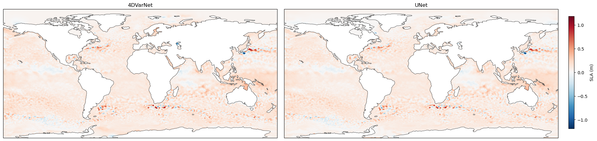
Figure 3 shows the SLA predicted by end-to-end neural ocean forecasts at leadtime 1 on January 18 2023. Figure 4 shows the evaluation metrics across leadtimes 0, 3 and 5 for the benhmarked neural emulators models, all compared to the baseline GLO12, with the colorbar corresponding to the respective relative gains in %. The 4DVarNet consistently outperforms baseline GLO12 and other state-of-the-art neural forecasts across the nRMSE SSH score. Performance remains robust over time, highlighting the stability of the model across diverse ocean regimes. Furthermore, 4DVarNet also improves the derived SSC, particularly improving the forecast of SSC angles compared to drifters velocity vectors, suggesting a more accurate capture of flow directions.

4.3 Regime-dependent performance
Tables 2–4 assess the performance of the benchmarked models across leadtimes 0, 3 and 5 and three oceanic regimes: coastal, offshore high variability, and offshore low variability regions. Here we inter-compare the benchmarked models against the observation‑based delayed-time product DUACS (Taburet et al.,, 2019). DUACS uses an Optimal Interpolation (OI) algorithm applied to sparse altimetry data (Ballarotta et al.,, 2019; Le Traon et al.,, 2025). We emphasize that, for a given leadtime, DUACS product exploits past and future altimetry observations. This is the reason why we do not include it in the benchmark among the tested approaches. It provides us with a means to compute relative performance metrics in our regime-dependent analysis. DUACS can better reflect the spatial structures of SLA compared to assimilation-based model analyses, especially in highly dynamic regions (Ballarotta et al.,, 2019).


To quantify forecasts’ accuracies relative to the DUACS baseline, we compute percentage gains of each metric relative to the corresponding DUACS score (both evaluated with respect to Saral/AltiKa observations), see Tables 2-4. At leadtime 0, 4DVarNet achieves the best performance compared to GLO12 baseline across all regions. It remains the closest to the DUACS reconstruction, and is even able to outperform it in offshore high-variability regions. UNet performs slightly worse than 4DVarNet, however outperforms GLO12, especially in coastal regions. GloNet underperforms 4DVarNet and UNet, while XiHe is at the same level of performance as GLO12, as its first leadtime is defined as the one provided by the reanalysis. At leadtime 3, 4DVarNet maintains strong performance across all regimes, consistently achieving the lowest RMSE and highest nRMSE, reaching positive gains relative to DUACS. UNet shows competitive performance in low-variability areas, but is worse than GloNet in coastal regions, which gains in performance compared to the first leadtime. By leadtime 5, 4DVarNet still consistently outperforms GLO12 across all regimes and is considerably outperforming DUACS reconstruction especially in coastal and offshore low-variance regions. UNet remains competitive especially in low-variance areas. Overall, all models lose performance relative to their first leadtime as forecasts advance, yet 4DVarNet keeping the lowest level of relative errors wrt DUACS, highlighting the ability of this end-to-end neural architecture to remain close to an observations-based short-term forecast even at longer leadtimes. Figures 6 and 5 further illustrates this comparison by displaying the SLA fields from GLO12, proposed end-to-end forecasts 4DVarNet and UNet at leadtimes 0 and 5, but also DUACS L4 product for the corresponding dates, in two high variability regions: Gulf Stream and Agulhas. As expected, GLO12 struggles to correctly position some dynamical structures in comparison to observation-based product DUACS. In the contrast, the end-to-end neural forecasts better recover spatial patterns and are more consistent with DUACS. At leadtime 5, however, the UNet forecast shows a noticeable loss of energy, reflected in a reduced SLA variance, a phenomenon which is not observed in the 4DVarNet forecasts.
| Coastal | Offshore High Var. | Offshore Low Var. | ||||
|---|---|---|---|---|---|---|
| Model | RMSE (%) | nRMSE (%) | RMSE (%) | nRMSE (%) | RMSE (%) | nRMSE (%) |
| GLO12 | 44.81 | 3.13 | 41.52 | 5.91 | 47.22 | 2.50 |
| GloNet | 52.26 | 3.64 | 52.54 | 7.48 | 57.33 | 3.04 |
| XiHe | 44.81 | 3.13 | 41.52 | 5.91 | 47.22 | 2.50 |
| 4DVarNet | 8.85 | 0.62 | -1.35 | -0.19 | 5.07 | 0.27 |
| UNet | 9.97 | 0.70 | 8.95 | 1.27 | 15.91 | 0.84 |
| Coastal | Offshore High Var. | Offshore Low Var. | ||||
|---|---|---|---|---|---|---|
| Model | RMSE (%) | nRMSE (%) | RMSE (%) | nRMSE (%) | RMSE (%) | nRMSE (%) |
| GLO12 | 49.23 | 3.52 | 54.25 | 7.72 | 55.51 | 2.97 |
| GloNet | 39.14 | 2.80 | 34.12 | 4.88 | 46.49 | 2.48 |
| XiHe | 130.18 | 9.32 | 183.34 | 26.14 | 157.44 | 8.41 |
| 4DVarNet | 11.20 | 0.80 | 5.37 | -0.77 | 9.14 | 0.49 |
| UNet | 20.47 | 1.46 | 19.49 | 2.78 | 22.79 | 1.21 |
| Coastal | Offshore High Var. | Offshore Low Var. | ||||
|---|---|---|---|---|---|---|
| Model | RMSE (%) | nRMSE (%) | RMSE (%) | nRMSE (%) | RMSE (%) | nRMSE (%) |
| GLO12 | 55.21 | 3.85 | 64.23 | 9.39 | 63.32 | 3.35 |
| GloNet | 48.19 | 3.37 | 35.46 | 5.21 | 50.37 | 2.67 |
| XiHe | 131.97 | 9.20 | 182.31 | 26.71 | 160.08 | 8.64 |
| 4DVarNet | 15.48 | 1.08 | 16.52 | 2.42 | 17.72 | 0.94 |
| UNet | 26.33 | 1.83 | 29.02 | 4.27 | 29.49 | 1.56 |


Figure 7 presents the relative gains of the benchmarked models with respect to the operational baseline forecast GLO12 for leadtime 0 for the explained variance metric calculated per bins. We refer the reader to the SSH mapping data challenge documentation for further details on the implementation of the metric. The gains are computed as the percentage difference relative to GLO12 for all scales as well as for spatial scales ranging between 65 and 500 km. Visually, the 4DVarNet model shows large improvements over the baseline across all scales. We observe the most significant added value in small scales (65–500 km), specifically in the offshore regions (both high and low variability), which we have already shown in the quantitative analysis in the Table 2. We suggest that the 4DVarNet forecast model is able to capture smaller dynamics due to its gradient regularization. Similarly, UNet also shows more improvements in the filtered maps, with a particular gain in ofsshore low variability regions, with a localized degradations along the equatorial band. In the contrast to the end-to-end neural forecasts, GloNet shows heterogeneous improvements wrt baseline GLO12 across the chosen metric, with a particular degradation of performances in coastal regions, and some improvements in higher latitudes. These spatial distributions of explained variance errors highlight that 4DVarNet provides the most consistent improvements globally, whereas UNet and GloNet show more heterogeneous performances. Furthermore, the more significant improvements at smaller scales underscores that the end-to-end neural forecasts can better exploit sparse observations to forecast dynamics at scales where traditional model-based forecast is less reliable.
5 Conclusion and Discussion
This study introduces a deep learning-based framework for short-term ocean forecasting, leveraging end-to-end neural architecture, especially 4DVarNet schemes, in a novel forecasting setup. Trained on simulated nadir altimetry data, the model demonstrates state-of-the-art performance in predicting global SSH over a 7-day horizon. Integrated within the OceanBench benchmarking initiative (Johnson et al.,, 2023; Aouni et al.,, 2025), our approach provides a standardized and reproducible framework for neural ocean forecasting. These results open promising avenues for future improvements in operational oceanography using machine learning. Our findings demonstrate the relevance of end-to-end neural networks for short-term ocean forecasting. The ability of 4DVarNet to handle sparse observations and to produce accurate forecasts is of particular interest for operational contexts, where real-time data are often incomplete or noisy.
While we only rely on training strategies based on reanalysis datasets and simulated observation data, future work could explore the potential of training schemes using real observation datasets (Martin et al.,, 2024; Dorffer et al.,, 2025). In this context, the benefit of wide-swath altimetry data could be highly valuable (Ballarotta et al.,, 2025; Fouchet et al.,, 2025). Accounting for uncertainty quantification in the proposed end-to-end neural forecasts is also a key challenge. We aim to explore the combination of 4DVarNet schemes and generative approaches (Li et al.,, 2024) as recently explored for SLA mapping (Beauchamp et al.,, 2025).
Acknowledgments
This work has been carried out as part of the Copernicus Marine Service OceanBench-STOF project. Copernicus Marine Service is implemented by Mercator Ocean in the framework of a delegation agreement with the European Union. This work was partially supported by the French ANR OceaniX (ANR-19-CHIA-0016). It also benefited from HPC and GPU resources provided by GENCI-IDRIS (Grant 2021-101030) and the CPER AIDA GPU cluster, supported by the Regional Council of Brittany, Brest Métropole, and Fonds Européen de DEveloppement Régional (FEDER).
References
- Aouni et al., (2025) Aouni, A. E., Gaudel, Q., Johnson, J. E., Charly, R., Sommer, J. L., van Gennip, Fablet, R., Drevillon, M., DRILLET, Y., and Traon, P. Y. L. (2025). Oceanbench: A benchmark for data-driven global ocean forecasting systems. In The Thirty-ninth Annual Conference on Neural Information Processing Systems Datasets and Benchmarks Track.
- Ashish, (2017) Ashish, V. (2017). Attention is all you need. Advances in neural information processing systems, 30:I.
- Ballarotta et al., (2025) Ballarotta, M., Ubelmann, C., Bellemin-Laponnaz, V., Le Guillou, F., Meda, G., Anadon, C., Laloue, A., Delepoulle, A., Faugère, Y., Pujol, M.-I., et al. (2025). Integrating wide-swath altimetry data into level-4 multi-mission maps. Ocean Science, 21(1):63–80.
- Ballarotta et al., (2019) Ballarotta, M., Ubelmann, C., Pujol, M.-I., Taburet, G., Fournier, F., Legeais, J.-F., Faugère, Y., Delepoulle, A., Chelton, D., Dibarboure, G., et al. (2019). On the resolutions of ocean altimetry maps. Ocean science, 15(4):1091–1109.
- Barth et al., (2020) Barth, A., Alvera-Azcárate, A., Licer, M., and Beckers, J.-M. (2020). Dincae 1.0: A convolutional neural network with error estimates to reconstruct sea surface temperature satellite observations. Geoscientific Model Development, 13(3):1609–1622.
- Beauchamp et al., (2021) Beauchamp, M., Amar, M. M., Febvre, Q., and Fablet, R. (2021). End-to-end learning of variational interpolation schemes for satellite-derived ssh data. In 2021 IEEE International Geoscience and Remote Sensing Symposium IGARSS, pages 7418–7421. IEEE.
- Beauchamp et al., (2025) Beauchamp, M., Fablet, R., Benaichouche, S., Tandeo, P., Desassis, N., and Chapron, B. (2025). Neural variational data assimilation with uncertainty quantification using spde priors. Artificial Intelligence for the Earth Systems, 4(3):240060.
- Bi et al., (2023) Bi, K., Xie, L., Zhang, H., Chen, X., Gu, X., and Tian, Q. (2023). Accurate medium-range global weather forecasting with 3d neural networks. Nature, 619(7970):533–538.
- Brasseur and Verron, (2006) Brasseur, P. and Verron, J. (2006). The seek filter method for data assimilation in oceanography: a synthesis. Ocean Dynamics, 56(5):650–661.
- Buizza et al., (2018) Buizza, R., Balmaseda, M. A., Brown, A., English, S., Forbes, R., Geer, A., Haiden, T., Leutbecher, M., Magnusson, L., Rodwell, M., et al. (2018). The development and evaluation process followed at ECMWF to upgrade the Integrated Forecasting System (IFS). European Centre for Medium Range Weather Forecasts.
- Cui et al., (2025) Cui, Y., Wu, R., Zhang, X., Zhu, Z., Liu, B., Shi, J., Chen, J., Liu, H., Zhou, S., Su, L., et al. (2025). Forecasting the eddying ocean with a deep neural network. Nature Communications, 16(1):2268.
- Cummings and Smedstad, (2013) Cummings, J. A. and Smedstad, O. M. (2013). Variational data assimilation for the global ocean. In Data assimilation for atmospheric, oceanic and hydrologic applications (Vol. II), pages 303–343. Springer.
- Davidson et al., (2009) Davidson, F. J., Allen, A., Brassington, G. B., Øyvind Breivik, Daniel, P., Kamachi, M., Sato, S., King, B., Lefevre, F., Sutton, M., and Kaneko, H. (2009). Applications of godae ocean current forecasts to search and rescue and ship routing. Oceanography, 22(3):176–181.
- Dorffer et al., (2025) Dorffer, C., Jourdin, F., Nguyen, T. T. N., Devillers, R., Mouillot, D., and Fablet, R. (2025). Observation-only deep learning for gappy satellite-derived ocean colour data using 4dvarnet. IEEE Transactions on Geoscience and Remote Sensing.
- Ducet et al., (2000) Ducet, N., Le Traon, P.-Y., and Reverdin, G. (2000). Global high-resolution mapping of ocean circulation from topex/poseidon and ers-1 and-2. Journal of Geophysical Research: Oceans, 105(C8):19477–19498.
- El Aouni et al., (2025) El Aouni, A., Gaudel, Q., Regnier, C., Van Gennip, S., Le Galloudec, O., Drevillon, M., Drillet, Y., and Lellouche, J.-M. (2025). Glonet: Mercator’s end-to-end neural global ocean forecasting system. Journal of Geophysical Research: Machine Learning and Computation, 2(3).
- Fablet et al., (2021) Fablet, R., Chapron, B., Drumetz, L., Mémin, E., Pannekoucke, O., and Rousseau, F. (2021). Learning variational data assimilation models and solvers. Journal of Advances in Modeling Earth Systems, 13(10).
- Fablet et al., (2023) Fablet, R., Febvre, Q., and Chapron, B. (2023). Multimodal 4dvarnets for the reconstruction of sea surface dynamics from sst-ssh synergies. IEEE Transactions on Geoscience and Remote Sensing, 61:1–14.
- Febvre et al., (2024) Febvre, Q., Le Sommer, J., Ubelmann, C., and Fablet, R. (2024). Training neural mapping schemes for satellite altimetry with simulation data. Journal of Advances in Modeling Earth Systems, 16(7).
- Febvre et al., (2023) Febvre, Q., Sommer, J. L., Ubelmann, C., and Fablet, R. (2023). Training neural mapping schemes for satellite altimetry with simulation data. arXiv preprint arXiv:2309.14350.
- Fennel et al., (2022) Fennel, K., Mattern, J. P., Doney, S. C., Bopp, L., Moore, A. M., Wang, B., and Yu, L. (2022). Ocean biogeochemical modelling. Nature Reviews Methods Primers, 2(1):76.
- Fouchet et al., (2025) Fouchet, E., Benkiran, M., Le Traon, P.-Y., and Remy, E. (2025). Comparison of a global high-resolution ocean data assimilation system with swot observations. Frontiers in Marine Science, 12:1563934.
- Garcia et al., (2025) Garcia, P., Larroche, I., Pesnec, A., Bull, H., Archambault, T., Moschos, E., Stegner, A., Charantonis, A., and Béréziat, D. (2025). Orcast: Operational high-resolution current forecasts. Artificial Intelligence for the Earth Systems.
- Hobday et al., (2016) Hobday, A. J., Alexander, L. V., Perkins, S. E., Smale, D. A., Straub, S. C., Oliver, E. C., Benthuysen, J. A., Burrows, M. T., Donat, M. G., Feng, M., et al. (2016). A hierarchical approach to defining marine heatwaves. Progress in oceanography, 141:227–238.
- Hoteit et al., (2024) Hoteit, I., Chassignet, E., and Bell, M. (2024). Improving accuracy and providing uncertainty estimations: ensemble methodologies for ocean forecasting. State of the Planet Discussions, 2024:1–11.
- Johnson et al., (2023) Johnson, J. E., Febvre, Q., Gorbunova, A., Metref, S., Ballarotta, M., Le Sommer, J., et al. (2023). Oceanbench: The sea surface height edition. Advances in Neural Information Processing Systems, 36:78275–78295.
- Lahoz and Schneider, (2014) Lahoz, W. A. and Schneider, P. (2014). Data assimilation: making sense of earth observation. Frontiers in Environmental Science, 2:16.
- Lam et al., (2022) Lam, R., Sanchez-Gonzalez, A., Willson, M., Wirnsberger, P., Fortunato, M., Alet, F., Ravuri, S., Ewalds, T., Eaton-Rosen, Z., Hu, W., et al. (2022). Graphcast: Learning skillful medium-range global weather forecasting. arXiv preprint arXiv:2212.12794.
- Le Traon et al., (2017) Le Traon, P.-Y., Dibarboure, G., Jacobs, G., Martin, M., Rémy, E., and Schiller, A. (2017). Use of satellite altimetry for operational oceanography. Satellite altimetry over oceans and land surfaces, pages 581–608.
- Le Traon et al., (2025) Le Traon, P.-Y., Dibarboure, G., Lellouche, J.-M., Pujol, M.-I., Benkiran, M., Drevillon, M., Drillet, Y., Faugère, Y., and Remy, E. (2025). Satellite altimetry and operational oceanography: from jason-1 to swot. Ocean Science, 21(4):1329–1347.
- Le Traon et al., (2019) Le Traon, P. Y., Reppucci, A., Alvarez Fanjul, E., Aouf, L., Behrens, A., Belmonte, M., Bentamy, A., Bertino, L., Brando, V. E., Kreiner, M. B., et al. (2019). From observation to information and users: The copernicus marine service perspective. Frontiers in marine science, 6:234.
- Lellouche et al., (2018) Lellouche, J.-M., Greiner, E., Le Galloudec, O., Regnier, C., Benkiran, M., Testut, C.-E., Bourdalle-Badie, R., Drevillon, M., Garric, G., and Drillet, Y. (2018). Mercator ocean global high-resolution monitoring and forecasting system. New Frontiers in Operational Oceanography, pages 563–592.
- Lellouche et al., (2023) Lellouche, J.-M., Greiner, E., Ruggiero, G., Bourdallé-Badie, R., Testut, C.-E., Le Galloudec, O., Benkiran, M., and Garric, G. (2023). Evolution of the copernicus marine service global ocean analysis and forecasting high-resolution system: potential benefit for a wide range of users. Proceeding Eurogoos, pages 242–251.
- Lellouche et al., (2013) Lellouche, J.-M., Le Galloudec, O., Drévillon, M., Régnier, C., Greiner, E., Garric, G., Ferry, N., Desportes, C., Testut, C.-E., Bricaud, C., et al. (2013). Evaluation of global monitoring and forecasting systems at mercator océan. Ocean Science, 9(1):57–81.
- Lermusiaux et al., (2006) Lermusiaux, P. F., Chiu, C.-S., Gawarkiewicz, G. G., Abbot, P., Robinson, A. R., Miller, R. N., Haley, P. J., Leslie, W. G., Majumdar, S. J., Pang, A., et al. (2006). Quantifying uncertainties in ocean predictions.
- Li et al., (2024) Li, L., Carver, R., Lopez-Gomez, I., Sha, F., and Anderson, J. (2024). Generative emulation of weather forecast ensembles with diffusion models. Science Advances, 10(13):eadk4489.
- Liu et al., (2023) Liu, G., Bracco, A., and Brajard, J. (2023). Systematic bias correction in ocean mesoscale forecasting using machine learning. Journal of Advances in Modeling Earth Systems, 15(11).
- Madec et al., (2015) Madec, G. et al. (2015). Nemo ocean engine.
- Martin et al., (2023) Martin, S. A., Manucharyan, G. E., and Klein, P. (2023). Synthesizing sea surface temperature and satellite altimetry observations using deep learning improves the accuracy and resolution of gridded sea surface height anomalies. Journal of Advances in Modeling Earth Systems, 15(5).
- Martin et al., (2024) Martin, S. A., Manucharyan, G. E., and Klein, P. (2024). Deep learning improves global satellite observations of ocean eddy dynamics. Geophysical Research Letters, 51(17).
- Ronneberger et al., (2015) Ronneberger, O., Fischer, P., and Brox, T. (2015). U-net: Convolutional networks for biomedical image segmentation. In International Conference on Medical image computing and computer-assisted intervention, pages 234–241. Springer.
- Shi et al., (2015) Shi, X., Chen, Z., Wang, H., Yeung, D.-Y., Wong, W.-K., and Woo, W.-c. (2015). Convolutional lstm network: A machine learning approach for precipitation nowcasting. Advances in neural information processing systems, 28.
- Taburet et al., (2019) Taburet, G., Sanchez-Roman, A., Ballarotta, M., Pujol, M.-I., Legeais, J.-F., Fournier, F., Faugere, Y., and Dibarboure, G. (2019). Duacs dt2018: 25 years of reprocessed sea level altimetry products. Ocean Science, 15(5):1207–1224.
- Wang et al., (2024) Wang, X., Wang, R., Hu, N., Wang, P., Huo, P., Wang, G., Wang, H., Wang, S., Zhu, J., and Xu, J. (2024). Xihe: A data-driven model for global ocean eddy-resolving forecasting. arXiv preprint arXiv:2402.02995.
- Xiong et al., (2023) Xiong, W., Xiang, Y., Wu, H., Zhou, S., Sun, Y., Ma, M., and Huang, X. (2023). Ai-goms: Large ai-driven global ocean modeling system. arXiv preprint arXiv:2308.03152.
