Expanding Asteroseismic Studies in Star Clusters Using NASA’s TESS and ESA’s Gaia Missions

Carli Mankowski Department of Astronomy, University of Florida, Gainesville, FL 32611, USA [ Jamie Tayar Department of Astronomy, University of Florida, Gainesville, FL 32611, USA jtayar@ufl.edu Cassidy Martin Department of Astronomy, University of Florida, Gainesville, FL 32611, USA cassidymartin@ufl.edu

Abstract

Star clusters have long been central to the study of stellar evolution due to their chemically and chronologically homogeneous populations. Asteroseismology, the analysis of stellar oscillations and pulsations, provides precise information about properties such as masses, radii, and ages of stars in the field. However, these stars lack calibration to an absolute scale, and so this project seeks to utilize the data from NASA’s TESS mission and ESA’s Gaia mission to identify additional cluster stars suitable for asteroseismic analysis and calibration. In this work we analyze 14 stars belonging to 3 well-populated clusters, 5 additional stars that are the only detected oscillators in their respective clusters, and 3 detected oscillators of unknown cluster membership. By significantly expanding the number of clusters with measured oscillating giants, this project increases the opportunity for cross-validation between classical stellar models and asteroseismic methods, allowing for improvements in both calibration techniques and age estimations across the galaxy.

Asteroseismology — Stellar oscillations — Open star clusters — Stellar evolutionary models — Stellar photometry — Stellar properties — Gaia — Stellar pulsations

show]carli.mankowski@ufl.edu

I Introduction

The determination of stellar age is foundational in our understanding of galactic formation. In order to accurately infer stellar ages, we need to be able to calibrate models using well-studied examples and observed data. Increasing our understanding of the relationship between stellar properties and age enables connections across diverse areas of astronomy. Ages can be combined with chemical diagnostics (Tucci Maia et al., 2016), nucleosynthetic pathway studies (Casali et al., 2022) and large-scale kinematic maps (Buder et al., 2021) to help reconstruct the Milky Way’s history. They also enhance chemical evolution models, improve stellar mass estimates, and inform other observational analyses (Stello and Sharma, 2023). Its large-scale applicability and long-standing academic scrutiny secure stellar age as a cornerstone diagnostic element of galactic study. Examples of the contextual applicability of stellar age include the topics of planetary system evolution (Yang et al., 2023), galaxy mergers (Horta et al., 2024), galactic chemical enrichment (Feuillet et al., 2018), and epochs of star formation (Thomas et al., 2005). Our very understanding of the Milky Way is a prime example of the integration of age estimations and observational constraints (i.e., photometric, spectroscopic, and kinematic diagnostics). Using the ages of galactic globular clusters allows us to study early formation; using the ages of non-primordial clusters allows us to study our galaxy’s accretion events from long ago (Ying et al., 2025). In this way, stellar age serves as a unifying metric for individual stellar histories and the evolution of stellar, galactic, and cosmological studies.

Star clusters have long been central to the study of stellar evolution because their chemically and chronologically homogeneous populations make them ideal laboratories for testing and calibrating age estimates and other theoretical models. This remains true across a diverse sample of masses and evolutionary stages (Miglio et al., 2021a). Using observational diagnostics such as color–magnitude diagrams (CMDs; Cantat-Gaudin and Anders (2020)) and theoretical isochrones (Reyes et al., 2024) can also aid in the determination of stellar properties across this same wide‑scale sample. Although star clusters have long served as key laboratories for testing and calibrating stellar-evolution and age-dating models, the majority of observable stars reside outside of bound clusters. Calibrating these models on cluster members then enables their application to field stars whose ages cannot be independently confirmed. Recent advances in asteroseismology have demonstrated the potential to infer ages for hundreds of thousands of field stars if their accuracy can be anchored to coeval benchmarks such as clusters (Hon et al., 2024; Theodoridis et al., 2025).

Asteroseismology is the study of stellar oscillation for the purpose of gaining insight into internal stellar structure (Brown et al., 1989; Kjeldsen and Bedding, 1995). Characterizing the frequencies of these resonant oscillations in solar-like oscillators provides insight into various properties such as stellar evolution (Chaplin and Miglio, 2013), stellar masses, radii, and luminosities (Hekker et al., 2011). Global asteroseismic observables include $\Delta\nu$ , the large frequency separation between overtone modes of the same angular degree, and $\nu_{\text{max}}$ , the frequency at which the oscillation power envelope reaches its maximum (Hekker et al., 2011). scillatory behavior is closely correlated with stellar mass and radius (Ash et al., 2024). Using asteroseismology with scaling relations (Hon et al., 2024) allows for accurate age estimation and is thus a gateway for quantitative progress in understanding stellar history and evolutionary timescales (Lebreton and Montalbán, 2008).

At this point, a variety of space-based photometry missions have provided the necessary data to characterize the asteroseismic oscillations of thousands of stars, and almost all of them have included subsets of stars in clusters that can be used for calibration. CoRoT (COnvection, ROtation and planetary Transits) (2006–2013) (Baglin et al., 2006) pioneered space-based asteroseismology by detecting thousands of red giant oscillations among solar-like stars (Mosser et al., 2018), and the Kepler mission (2009–2013) (Borucki et al., 2010) subsequently revealed tens of thousands more oscillators in a similar stellar sample (Yu et al., 2018). The K2 campaign (2014–2018) (Howell et al., 2014) included cluster members, giants, and a few dwarf stars through thousands of detections (Zinn et al., 2022), while TESS (2018–present) (Ricker et al., 2015) has surveyed the bright all-sky field and identified over 158,000 oscillators, predominantly red giants (Hon et al., 2021).

Combining asteroseismology with supplemental information such as Gaia photometry (Risbud et al., 2025; Myers et al., 2022) and cluster membership (Hunt and Reffert, 2023a; Tayar and Joyce, 2025) can expand the impact of asteroseismology and constrain the chemical and dynamical evolution of stars; integration of these large, consistent datasets allows for deeper comparative analysis. However, their age estimations are still at odds with those derived from isochrone fitting (Tayar and Joyce, 2025; Palakkatharappil and Creevey, 2023).

In this context, NASA’s TESS mission, launched on 2018 April 18, provides nearly all-sky high-precision photometry. TESS operates in a 27.4-day highly elliptical Earth orbit, observing consecutive ( $24^{\circ}\times 96^{\circ}$ ) sectors (Ricker et al., 2015) and delivering both light curves and full-frame images (FFIs) (Stassun et al., 2019c), ultimately achieving continuous coverage of more than 95% of the sky (Jenkins et al., 2016). We can now also advance asteroseismic studies using TESS data due to its all-sky coverage of many targets with high precision. Since TESS provides asteroseismic data for solar-type stars (Ricker et al., 2015) all over the sky, it opens the possibility of greatly increasing the number of clusters with asteroseismic data that could then be used to calibrate the ages of hundreds of thousands of oscillators across the galaxy. Prior to this work, asteroseismic detections in giant stars had been reported in only seven open clusters and six globular clusters ( Edmonds and Gilliland (1996); Stello and Gilliland (2009); Howell et al. (2024); see also Miglio et al. (2021a) for a review). Our analysis of TESS data adds eight open clusters, three well-populated and five with single detections, more than doubling the known sample of open clusters with seismically characterized giants.

However, the fundamental operation of TESS can impose certain limitations that can impair the study of asteroseismology. Since TESS has a large pixel size, light from nearby sources can contaminate that of target stars, especially in crowded fields, complicating the extraction of clean light curves for individual stars (Hatt et al., 2023). Additionally, upon its initial launch, TESS’s 30-minute cadence imposed a Nyquist frequency limit of $278\text{\,}\mathrm{\SIUnitSymbolMicro Hz}$ : the highest frequency that can be accurately sampled without aliasing, which may affect the asteroseismology of stars with oscillation frequencies at or around that Nyquist limit (Murphy, 2015; Barclay et al., 2020). TESS also faces analytical limitations, including lost detections caused by data gaps and short observing sectors (Guerrero and others, 2021) and challenges arising from its month-to-month discontinuous observing pattern (Lu et al., 2020).

Therefore, to promote the efficient analysis of TESS asteroseismology in star clusters, we aim to establish a database of cluster stars that are suitable for seismic analysis, even with the limitations of the TESS mission as described above. For example, we are interested in whether the ages derived from global asteroseismic parameters are consistent with cluster ages obtained from isochrone fitting. Previous work has suggested that seismically inferred ages may differ systematically from those obtained using other techniques, often yielding larger values (Tayar and Joyce, 2025). However, the small number of clusters analyzed to date, together with their limited coverage in metallicity and age, makes it difficult to assess the true accuracy and precision of ages inferred from asteroseismology.

In this study we combine precise astrometry, membership information, and isochrone-based ages for nearby open clusters from the Gaia mission with all-sky photometric data from TESS. We demonstrate that, despite the relatively short time series and large pixel scale of TESS, its data are sufficient in many cases to characterize the oscillations of red giant cluster members. We then compare ages inferred from asteroseismic scaling relations and stellar age modeling to literature cluster parameters in order to map the reliability of seismic ages, enabling their broader application to infer the ages of large samples of field stars across the Milky Way (Theodoridis et al., 2025). To facilitate future work, we provide a catalog of cluster stars that may be suitable for seismic analysis with TESS.

II Methods

II.1 Catalog Selection

The foundation of this work relies on careful characterization and association of cluster stars. We use Gaia DR3, whose all-sky parallaxes, proper motions, magnitudes, BP-RP colors, and other photometry allow for accuracy in determining open-cluster membership, precise distances, and clean HR-diagram placement (Gaia Collaboration et al., 2023). This photometric data is pulled from cluster membership studies such as Hunt and Reffert (2023a), Schiavon et al. (2022), and Cantat-Gaudin and Anders (2020), which have already grouped members of the same clusters together with reasonable confidence.

Using the Hunt and Reffert (2023a), Schiavon et al. (2022), and Cantat-Gaudin and Anders (2020) catalogs, we queried the TESS Input Catalog (TIC v8; Stassun et al. 2019c) via the S3 STScI public dataset using astroquery.mast.cloud to isolate targets with unique TIC IDs. To account for systematic errors such as field variation, cosmic noise, and electro-optical response differences (Gai et al., 2022), the right ascension and declination of each target were given a radial error window of 0.1 degrees. After confirming that each target was present in the TESS Input Catalog, we performed a column-wise merge to match Hunt and Reffert (2023a), Schiavon et al. (2022), and Cantat-Gaudin and Anders (2020) members with a CSV file containing TIC IDs from the 2019 TIC-7 Input Catalog (Stassun et al., 2019a). These two datasets were merged on a shared identifier column (Gaia DR3), producing a functional catalog of stars with secure membership classifications and relevant astrometry. This catalog contains 38311 members for further consideration, all within the TESS input catalog.

II.2 Distance Cuts

We filter our catalog to eliminate distant targets, following the findings of Cantat-Gaudin and Anders (2020), which concluded that Gaia DR3 proper motion uncertainties contribute at $\sim$ $500\text{\,}\mathrm{pc}$ and dominate at distances beyond $1000\text{\,}\mathrm{pc}$ . Using the identity $d=\frac{1000}{\varpi}$ , where $d$ is the distance in parsecs and $\varpi$ is the parallax in milliarcseconds, we use catalog-provided parallax data to remove any stars at distances greater than $1\text{\,}\mathrm{kpc}$ . This reduces the systematic noise and measurement uncertainty from the dataset. Filtering out distant stars leaves a nearby sample with more reliable absolute magnitudes, because parallax-based distance uncertainties and absolute-magnitude uncertainties are typically a factor of $\sim 5$ –10 smaller for stars within a few kiloparsecs than for more distant objects (Lindegren and others, 2018).

II.3 Magnitude Filtering

We take into consideration the intense “bleeding” effect of bright stars on TESS’s camera in the creation of our catalog. Stars that are exceptionally bright will not yield any photometric data, as the TESS pipeline does not process anything past its brightness threshold (TESS Science Processing Operations Center, 2025). For targets under that threshold, we cannot extract reliable brightness data from stars whose light bleeds into multiple pixels, introducing the need for a “cap” on how bright a star can be. This is explored further in section §II.5. We use the TESS QLP Aperture Lightcurve Products, which are generated only for stars brighter $T\approx 13.5$ and can exclude the very brightest targets when bleed-trail pixel stamps preclude standard processing (MIT TESS Science Office, 2025; Fausnaugh and the TESS Team, 2023).

We also account for the increased contamination and background noise affecting fainter TESS targets, which becomes a significant issue beyond $G\sim 15$ and renders stars fainter than $G\gtrsim 16$ largely unsuitable for precise asteroseismology (Riello et al., 2021; Boyle et al., 2025). Following previous asteroseismic work and Stassun et al. (2019b), we restrict our sample to stars with $G\leq 13$ mag so solar-like oscillations can be reliably detected at high signal-to-noise and to prioritize high signal-to-noise targets for analysis (Hon et al., 2021; Boyle et al., 2025; Zhou et al., 2024; Grusnis et al., 2025).

II.4 Color Magnitude Diagrams and Red Giant Selection

We require all stars in our sample to have reported Gaia photometry (G and $G_{\rm BP}-G_{\rm RP}$ ). To obtain these values, we merge the cluster member list with the Gaia DR3 photometric catalog of Andrae et al. (2023). This addition allows us to construct a color–magnitude diagram (CMD) that traces the evolutionary state of each star (Gaia Collaboration et al., 2018). Following the methods of Konchady (2020), we create a CMD from the mean G-band magnitude (G) and color index $(G_{\rm BP}-G_{\rm RP})$ provided by the XGBoost-based Gaia DR3 catalog. In our analysis, this XGBoost catalog is used for the photometry and atmospheric parameters ( $T_{\mathrm{eff}}$ , [Fe/H], and $\log g$ ). Where these values are missing or physically unrealistic, we use atmospheric parameters adopted from the gspec spectroscopic catalog. By applying the distance modulus,

M_{G}=G-5\log_{10}(d)+5,

(1)

we convert all of the Gmag values in the catalog ( $G$ ) into the absolute magnitude $M_{G}$ .

This catalog follows the selection principles of Hon et al. (2021) and Stello et al. (2022), prioritizing red giants because their solar-like oscillations have larger amplitudes and are detected at higher rates in TESS data. Since red giants span a broad range of stellar ages (Xiang et al., 2022), this should allow us to test the reliability of seismically inferred ages more generally. We visualize the full sample on a Gaia-based CMD (Figure 1) and we also show the three most populated clusters with seismic detections in our sample, Casado Alessi-1, Theia 6046, and NGC 752 (Figure 2). We approximate the location of the main sequence in this diagram in order to exclude stars that are unlikely to be red giants. To do this, we define an empirical main-sequence locus in color–magnitude space and remove stars that fall close to this sequence rather than on the red giant branch. The main sequence line used in our CMD approximation is given by $M_{G}=3.5\times(BP-RP)$ where $M_{G}$ is the absolute Gaia G-band magnitude and $BP-RP$ is the Gaia color index. In order to be fairly confident that our sample only contains red giants, we filter this CMD so that each target greater than 3.5 units of magnitude away from the main sequence line in the $+y$ direction is deemed a potential red giant. Out of the initial sample of 38,311 distance and magnitude corrected stars, 986 are estimated to be potential red giants and the other 37,667 are estimated to be potential main sequence.

Refer to caption — Figure 1: Global HR diagram using (Gaia) absolute magnitude vs BP-RP color. Main sequence stars are shown in blue, potential red-giants in red, seismic detections marked as green stars, and the main sequence approximated by the black dashed line.

II.5 Crowding, Bleeding and Duration Requirements

TESS’s observing pattern, large pixels, and susceptibility to saturation around the brightest stars can result in a degradation of data quality that makes seismic analysis challenging or impossible. This suggests that not every cluster red giant in our sample will have the quality of data needed to perform asteroseismology. For this analysis, we want to focus on stars with clean point-spread functions and sufficient data. To address this, we individually inspect each potential star to ensure the TESS data exist. Then, we check if nearby stars allow for the extraction of a clean light curve, or if local saturation and bleeding would result in the need for more advanced light curve techniques (Pope et al., 2016). Specifically, we used each star’s right ascension (RA), declination (Dec), and Gaia DR3 name to create a 10x10 pixel cutout around each target star using NASA’s Timeseries Integrated Knowledge Engine (TIKE). Nearby bright neighbors present the possibility for contaminated light-curves; we identified extraneous stars within both 3 magnitudes and 2 arcminutes of our target. We marked those nontarget stars to evaluate potential contamination of seismic signals.

For each star in our sample, we compiled individual identification information as well as visual inspection ratings into a table. Ratings were allocated to each target using a 1 to 5 scale with 5 representing the cleanest data. Several stars had no available sectors, these are marked with “-1” in the table and are not considered for further analysis. To create these visualizations, the first available sector was used. Exceptions were made for scenarios in which the target was either excessively faint or on the edge of the detector, and the next suitable sector was used. In Figure 3, we show representative cutouts with fixed bleeding and varying levels of crowding, and the impact of varying bleeding values at fixed crowding levels. Our full table of results is available on Zenodo, and the code to generate these cutouts can be found here.

We restricted our sample to stars with bleeding and crowding values of at least 2 and at least five available sectors. Only this subset of red giants was used in the subsequent analysis, though results for all targets are provided for reference and to enable future work. All quality cuts up to this point are replicable and the process is outlined on GitHub.

II.6 TESS Light Curve Retrieval and Pre-Processing

We then retrieved the raw light curves for the targets that had adequate bleeding, crowding, and sector metrics. Using the lk.search_lightkurve function, we located each TESS light curve from the QPL pipeline and downloaded them. For each sector, we normalized and flattened the data with a 299-cadence window, and removed $2.75\sigma$ outliers. We then stitched all available sectors into a single light curve and sorted the points by time (Jenkins et al., 2016). To avoid large gaps between sectors in the analysis, whenever we encountered a gap larger than 10 days in the time array, we subtracted the size of that gap from all subsequent time stamps to form a continuous time series for Fourier analysis, though we note potential biases for larger gaps as discussed in Bedding and Kjeldsen (2022). This pre-processing is an essential prerequisite to TESS data analysis, since the high values of systematic noise can damage results. The light curves were converted into power spectra, oversampled by a factor of five to achieve a frequency resolution of $\sim 0.1\,\mu$ Hz. The spectra were binned, using five-point binning for $\nu_{\max}$ estimation and 25-point binning for background fitting, following methods presented in Chontos et al. (2022b).

II.7 PySYD Seismic Analysis

Using PySYD, an open-sourced Python adaptation of the SYD method, we aimed to have code automatically detect the asteroseismic parameters $\nu_{\max}$ and $\Delta\nu$ . As noted in Huber and others (2009), the underlying SYD methodology was commonly used to measure oscillatory parameters in Kepler stars. Extending this to TESS, we needed to neutralize the noisy data with Gaussian smoothing of the oscillation power excess, an approach motivated by Huber and others (2009) and justified by Hon et al. (2024). We set 50 Monte Carlo iterations, restricted $\nu_{\max}$ to 1–100 $\mu$ Hz initially, refined the power spectrum to 10–60 $\mu$ Hz, and fitted the background between 5–525 $\mu$ Hz. Running PySYD produced $\nu_{\max}$ and $\Delta\nu$ estimates, background model fits, uncertainties, and diagnostic plots. Window restrictions were adjusted appropriately for each target, and uncertainties for $\nu_{\max}$ were calculated considering both PySYD values and visual inspection, referring to how far in each direction can be feasibly interpreted as $\nu_{\max}$ . Our typical fractional uncertainty on $\nu_{\max}$ is 3.3 $\%$ , comparable to the APOKASC-3 values reported by Pinsonneault et al. (2025). The Jupyter notebook used to run this PySYD analysis is openly available on GitHub.

Figure 4 is a visual demonstration of the workflow we follow to extract $\nu_{\max}$ from the TESS data. Starting from the detrended light curve (panel a), we compute the power spectrum and fit a background model that accounts for granulation, stellar activity, and white noise (panel b). After subtracting this background (panel c), the oscillation power excess becomes clearly visible. We then smooth the background‑corrected spectrum and fit a Gaussian to the oscillation envelope to determine $\nu_{\max}$ (panel d, dashed line). This same procedure is applied consistently to all targets.

II.8 Échelle Diagram Construction and Validation

To ensure that we report the most accurate $\Delta\nu$ values, we created two different interactive Échelle diagrams: a 2D heatmap and a collapsed ridge alignment strip (See Figure 5), using the Hey and Ball (2020b) code as a base and starting point. These all operate within a $\pm 2\Delta\nu$ window around $\nu_{\max}$ and are adjustable using a Bokeh package Custom JavaScript (JS) slider which instantaneously populates the graph with $\Delta\nu$ values as the slider is manipulated. Each target was passed through both plots, inspected, and the best $\Delta\nu$ was recorded along with more accurate uncertainties, referring to how far in each direction can be feasibly interpreted as $\Delta\nu$ . Our typical fractional uncertainty on $\Delta\nu$ is 2.26 $\%$ , comparable to the APOKASC-3 values reported by Pinsonneault et al. (2025).

In Figure 5, the diagnostic purpose is ridge coherence. With the adopted $\Delta\nu$ , the oscillation power repeats at consistent $\nu\bmod\Delta\nu$ from one radial order to the next, yielding clearly defined, near-vertical mode ridges in the 2D heatmap and corresponding concentrated columns in the collapsed strip. Although the spectrum is noisy, the ridge alignment remains stable across the $\pm 2\Delta\nu$ window around $\nu_{\max}$ , providing a visual confirmation that the measured $\Delta\nu$ captures the underlying comb-like spacing; perturbing $\Delta\nu$ visibly degrades this coherence by introducing ridge drift and broadening the collapsed power. The Jupyter notebook used to produce all Échelle figures and $\Delta\nu$ estimates is openly available on GitHub.

Figure 5: Échelle diagnostics for TIC 306552813 with adopted large separation

\Delta\nu=6.479~\mu\mathrm{Hz}

. Panel (a) shows the collapsed/overlay representation: the power spectrum is folded by

\Delta\nu

(x-axis: frequency modulo

\Delta\nu

) and collapsed across the displayed

\pm 2\Delta\nu

window; the collapse is replicated in y for visualization. Panel (b) shows the 2D échelle: x is frequency modulo

\Delta\nu

and y is an order index spanning the

\pm 2\Delta\nu

window around

\nu_{\max}

. Mode ridges appear as near-vertical bands of enhanced power in the 2D échelle; for this target the most prominent vertical bands are concentrated near

\nu\bmod\Delta\nu\approx 0.5~\mu\mathrm{Hz}

\nu\bmod\approx 3.2

–

3.6~\mu\mathrm{Hz}

, and

\nu\bmod\approx 5.3

–

5.4~\mu\mathrm{Hz}

. These same x-locations correspond to the strongest columns in the collapsed/overlay panel.

II.9 Evolutionary State Determination, Corrections, and Scaling Relations

In order to apply the appropriate corrections to the $\Delta\nu$ estimates, we first identified the evolutionary state of each star. While in some cases it is possible to infer the evolutionary state directly from the oscillations(Mosser et al., 2012; Vrard et al., 2025; Elsworth et al., 2019), this is challenging in low signal to noise cases like our data. Therefore, we infer evolutionary states from the Gaia color-magnitude diagram here, although future work may be able to improve upon this looking at each cluster in detail. Using the Gaia color–magnitude diagram, we tagged stars as red clump (RC) if they lay within a conservative rectangular region centered on the RC overdensity, using RC_COLOR_MIN, RC_COLOR_MAX = 0.9, 1.3 in $(BP{-}RP)$ and RC_MG_MIN, RC_MG_MAX = 0.2, 1.0 in $M_{G}$ . Gaia’s FLAME radii are the stellar radii estimated by the Gaia DR3 FLAME module, which combines bolometric fluxes, effective temperatures, and parallaxes (Gaia Collaboration, 2022), and has been used for population studies (Andrae et al., 2023). Applying the same selection box to an M67 Gaia CMD constructed from FLAME radii shows that it also cleanly traces the observed RC overdensity in that open cluster and shows that our cuts are consistent with well-behaved benchmark populations (Figure 6). We feel this box is an appropriate approximation for the compact RC feature near $(BP{-}RP)\!\approx\!1.1$ and $M_{G}\!\approx\!0.6$ visible in Gaia DR3 HRDs (Gaia Collaboration et al., 2018, their Fig. 10). The approximation also parallels the RC calibrations in Gaia bands that map $M_{G}$ (Figure 6) as a function of color in (Ruiz-Dern et al., 2018) and the GaiaUnlimited example that selects RC stars by cutting around a fiducial RC ridge line in the Gaia CMD (Gaia Collaboration et al., 2018). Evolutionary states were utilized in the application of model-based large-separation corrections $f_{\Delta\nu}$ , calculated using asfgrid interpolations over stellar-models as a function of evolutionary state, $T_{\rm eff}$ , [Fe/H], and the raw $(\Delta\nu,\nu_{\max})$ (Sharma et al., 2016; Stello and Sharma, 2023; Sharma et al., 2022).

To integrate our PySYD measurements into a community-average scale, we used the mean SYD-to-ensemble ratios $(X_{\Delta\nu},X_{\nu_{\max}})$ from the APOKASC-3 inter-pipeline calibration and the sub-percent PySYD $\leftrightarrow$ SYD consistency (Pinsonneault et al., 2025; Chontos et al., 2022b; Grusnis et al., 2025; Marasco et al., 2025). We note that the APOKASC-3 calibration factors are defined as the consensus value divided by the pipeline value, which is the reciprocal of the original definition of the correction factor used in White et al. (2011) and Sharma et al. (2016). We therefore take the reciprocal of the APOKASC-3 factors to obtain $X_{\Delta\nu}$ and $X_{\nu_{\max}}$ , so that they represent the factor by which the pipeline value must be divided to bring it onto the consensus scale. This aligns with the definition of the model-based correction $f_{\Delta\nu}$ from asfgrid.

We computed corrected parameters using

	$\displaystyle\Delta\nu_{\rm corr}$	$\displaystyle=\frac{\Delta\nu_{\rm pySYD}}{X_{\Delta\nu}\,f_{\Delta\nu}},$
	$\displaystyle\nu_{\max,{\rm corr}}$	$\displaystyle=\frac{\nu_{\max,{\rm pySYD}}}{X_{\nu_{\max}}\,f_{\nu_{\max}}},$

where $f_{\nu_{\max}}$ is a small adjustment derived by aligning seismic radii with Gaia-based radii after the $\Delta\nu$ scale is fixed. After observation of Figure 10, $f_{\nu_{\max}}$ is given a value of 1 since no meaningful correction was deemed necessary. This is consistent with our expectations for $f_{\nu_{\max}}$ around solar metallicity (Lindsay et al., 2025).

The corrected seismic parameters were then propagated through the standard scaling relations, with evolutionary-state dependent correction factors applied. Stellar radius and mass were computed as

	$\displaystyle\frac{R}{R_{\odot}}$	$\displaystyle=\left(\frac{\nu_{\max,{\rm corr}}}{\nu_{\max,\odot}}\right)\left(\frac{\Delta\nu_{\rm corr}}{\Delta\nu_{\odot}}\right)^{-2}\left(\frac{T_{\rm eff}}{T_{\rm eff,\odot}}\right)^{1/2},$
	$\displaystyle\frac{M}{M_{\odot}}$	$\displaystyle=\left(\frac{\nu_{\max,{\rm corr}}}{\nu_{\max,\odot}}\right)^{3}\left(\frac{\Delta\nu_{\rm corr}}{\Delta\nu_{\odot}}\right)^{-4}\left(\frac{T_{\rm eff}}{T_{\rm eff,\odot}}\right)^{3/2}.$

Here, $\nu_{\max,{\rm corr}}$ and $\Delta\nu_{\rm corr}$ are the corrected parameters defined above, incorporating both the empirical SYD-to-ensemble calibration factors $(X_{\nu_{\max}},X_{\Delta\nu})$ and the model-based $f_{\Delta\nu}$ correction together with the empirical $f_{\nu_{\max}}$ factor. The solar reference values $(\nu_{\max,\odot},\Delta\nu_{\odot},T_{\rm eff,\odot})$ adopted in this work are identical to those used in the APOKASC-3 calibration to maintain consistency across pipelines (Pinsonneault et al., 2025).

II.10 Seismic Radii

We determine stellar radii from asteroseismic scaling relations §II.9 with uncertainties from §II.13. For validation, we report them against external constraints. We use the Gaia DR3 FLAME catalog radii for red giants in the benchmark open cluster M67; these radii are derived from Gaia parallaxes and inferred angular diameters/stellar parameters (i.e., not seismic). The detailed FLAME comparison and our empirical re-calibration of radius uncertainties are presented in §II.13.2.

II.11 Seismic Masses and Cluster-wise Reporting

We determine stellar masses from asteroseismic scaling relations §II.9 with uncertainties from §II.13. For validation, we report the seismic mass distributions of three clusters (Casado Alessi-1, NGC 752, and Theia 6046), each target plotted against the masses of other members of the same cluster (Figure 11). This graphical analysis assesses internal, co-eval consistency rather than comparison to an external reference. In computing the cluster means and medians shown, we exclude the single Theia 6046 outlier (shown in Figure 11). Stars present in our broader sample but not confirmed as members of these three clusters are not plotted and do not enter the cluster-level statistics, but their seismic masses are included in the catalog.

II.12 Stellar Age Estimation

To estimate ages for our red giant cluster members, we use the age modeling tools in Kiauhoku (Claytor, 2020; Claytor et al., 2020). The process compares each star to four different sets of stellar-evolution models following the multi-model strategy suggested by Pinsonneault et al. (2025), with the individual models taken from YREC (Tayar et al., 2022), Dartmouth/DSEP (Dotter et al., 2008), GARSTEC (Weiss and Schlattl, 2008; Serenelli et al., 2013), and MIST (Choi et al., 2016). We use EEP-based tracks so that evolutionary stages are defined in a consistent way across all models. These models span the mass and metallicity ranges expected for our open clusters and let us test how different model assumptions affect red giant age estimates (Morales et al., 2025). For each star, we provide Kiauhoku with the observed quantities it can compare directly to the models: asteroseismic mass, $\log g$ , and metallicity. Kiauhoku then interpolates within each model and computes a $\chi^{2}$ measure of how well the model matches the observed values. These $\chi^{2}$ values are turned into likelihood weights, and we construct an age distribution for each by marginalizing over the weighted models. We emphasize that, given the specific set of inputs provided to Kiauhoku, this procedure is a deterministic grid lookup and interpolation rather than a Bayesian inference. For the final age estimate of each star, we use MIST as our primary model. The Dartmouth, YREC and GARSTEC models are used as comparison models, and we report their mean ages to allow direct comparison with other work. Since different model families can give ages that differ (Theodoridis et al., 2025; Tayar et al., 2022; Morales et al., 2025; Pinsonneault et al., 2025), using multiple models provides an estimate of the model-dependent uncertainty. This systematic age uncertainty is then added in quadrature to the observational age uncertainty, which we infer by perturbing the input mass and metallicity by $\pm 1\sigma$ following the procedures of Theodoridis et al. (2025) and Morales et al. (2025). The Jupyter notebook used to produce all age estimations is openly available on GitHub.

II.12.1 Cluster-Level Age Estimation

For each star, the MIST stellar-evolution grid in Kiauhoku returns an age estimate $t_{i}$ in Gyr. We define the cluster age as the arithmetic mean of the member-star ages,

\bar{t}=\frac{1}{N}\sum_{i=1}^{N}t_{i}.

(2)

This quantity represents the characteristic red-giant age of the cluster as inferred from the MIST models, and we adopt $\bar{t}_{\mathrm{MIST}}$ as our final seismic cluster age.

II.13 Error Propagation

We propagated uncertainties with first-order partial-derivative error propagation, assuming independent inputs. We describe (i) how we defined the measurement uncertainties on $\nu_{\max}$ and $\Delta\nu$ from PySYD and by-eye checks, (ii) how these propagate into radius and mass and are tested against catalog radii, and (iii) how we constructed the final age error bars at both the stellar and cluster levels.

II.13.1 Seismic Measurement Uncertainties from PySYD and By-Eye Checks

For each star, we first measured $\nu_{\max}$ and $\Delta\nu$ with PySYD and then inspected the power spectra by eye to confirm that the reported peaks and uncertainties were reasonable. The adopted $\sigma_{\nu_{\max}}$ and $\sigma_{\Delta\nu}$ reflect the formal PySYD uncertainties, moderated by manual checks. Uncertainties in $T_{\mathrm{eff}}$ , $\log g$ , and $[\mathrm{Fe}/\mathrm{H}]$ were taken directly from the relevant photometric or spectroscopic catalogs.

We treat $\nu_{\max}$ , $\Delta\nu$ , and $T_{\mathrm{eff}}$ as independent input quantities in the standard asteroseismic scaling relations. Using a first-order (Gaussian) Taylor expansion in $\ln X$ . Applying standard error propagation yields the expressions below.

Seismic mass error propagation:

$\left(\tfrac{\sigma_{M}}{M}\right)^{2}=9\left(\tfrac{\sigma_{\nu_{\max}}}{\nu_{\max}}\right)^{2}+16\left(\tfrac{\sigma_{\Delta\nu}}{\Delta\nu}\right)^{2}+\tfrac{9}{4}\left(\tfrac{\sigma_{T_{\rm eff}}}{T_{\rm eff}}\right)^{2}$

Seismic radius error propagation:

$\left(\tfrac{\sigma_{R}}{R}\right)^{2}=\left(\tfrac{\sigma_{\nu_{\max}}}{\nu_{\max}}\right)^{2}+4\left(\tfrac{\sigma_{\Delta\nu}}{\Delta\nu}\right)^{2}+\tfrac{1}{4}\left(\tfrac{\sigma_{T_{\rm eff}}}{T_{\rm eff}}\right)^{2}$

Seismic surface gravity error propagation:

$\left(\tfrac{\sigma_{g}}{g}\right)^{2}=\left(\tfrac{\sigma_{\nu_{\max}}}{\nu_{\max}}\right)^{2}+\tfrac{1}{4}\left(\tfrac{\sigma_{T_{\rm eff}}}{T_{\rm eff}}\right)^{2}$

II.13.2 FLAME-Based Radius Error Calibration

To validate our seismic radius scale and calibrate realistic radius uncertainties, we compare the scaling–relation radii to Gaia DR3 FLAME catalog values (Gaia Collaboration, 2022). In the benchmark open cluster M67, the published FLAME radii for 18 coeval giants show a residual distribution compared to the radii in Reyes et al. (2024), where we plot $(R_{\rm seis}-R_{\rm\textit{FLAME}})/\sigma_{\rm\textit{FLAME}}$ for M67 giants. The broad and asymmetric shape of this distribution represents underestimated uncertainties in the FLAME radii. To promote realistic radius errors in our analysis, we adopt an uncertainty of $\pm 2.0\,\sigma$ of the FLAME-reported uncertainty for red-giant radii. This data-driven treatment of the scatter provides the most straightforward and conservative set of error bars while remaining consistent with our seismically derived radius estimates. Because these systematics are significant, we regard the Reyes et al. (2024) seismic radii as the most accurate and up-to-date radius determinations available for these stars, and we use them as our reference scale.

II.13.3 Age Uncertainties at the Stellar and Cluster Levels

For each star, we define age uncertainties by rerunning the Kiauhoku fits after shifting the input mass and metallicity by their $\pm 1\sigma$ errors. The resulting changes in the recovered ages capture the observational contribution to the age error (through mass and metallicity). We then add in quadrature the spread in age between the different stellar-evolution grids at fixed star to account for model dependence. The stellar age uncertainty can be written as

\sigma_{t,\,\star}^{2}=\sigma_{\rm obs}^{2}+\sigma_{\rm model}^{2},

(3)

where $\sigma_{\rm obs}$ comes from perturbing the input mass and metallicity and $\sigma_{\rm model}$ reflects the grid-to-grid dispersion for that star. These $\sigma_{t,\,\star}$ values set the error bars on all star-by-star age plots. At the cluster level, the MIST grid provides a single mean age for the member stars (Section II.12.1) and an associated uncertainty that reflects both the typical stellar age errors and the scatter of ages within the cluster. We therefore adopt the MIST cluster age, $t_{\mathrm{MIST}}$ , as our final seismic age and assign an uncertainty

\sigma_{\mathrm{MIST}}^{2}=\frac{1}{N^{2}}\sum_{i=1}^{N}\sigma_{i}^{2}+s_{\mathrm{star}}^{2},

(4)

where $\sigma_{i}$ is the age uncertainty for star $i$ , and $s_{\mathrm{star}}$ is the sample-standard deviation of the member-star ages. In practice, the quoted $t_{\rm MIST}\pm\sigma_{\rm MIST}$ captures both uncertainty in the stellar inputs and the intrinsic spread of inferred ages within each cluster.

III Analysis

III.1 Catalog Presentation

We begin by presenting the full sample of stars selected for this study, including their basic astrometric and spectroscopic parameters. The catalog is constructed from Gaia DR3 and cross-matched with TESS Input Catalog identifiers. A sample of the full table is presented as Table A1. We illustrate the sample in a color–magnitude diagram (CMD) as a consistency check in Figure 1. This catalog includes columns which indicate whether or not a target has “passed” each cut, marked with ”y” for yes and ”n” for no. They are organized so that targets with the most “y”s are at the top and the least at the bottom, ensuring simplicity when searching for high quality targets. The full machine-readable catalog is available on Zenodo.

III.1.1 Unknown Clusters

The clusters marked as ”Unknown 1” (TIC306552754) and ”Unknown 2” (TIC306552795) in the catalog were both designated as ”Casado Alessi-1” in the Hunt and Reffert (2023a) paper, but upon examination of another focused cluster membership study (Cantat-Gaudin and Anders, 2020), we determined that they are likely non-members. A third source, ”Unknown 3” (TIC459055617), originally tagged as an NGC 2682 (M67) member, but the target is not analyzed by Reyes et al. (2025) and its asteroseismic parameters place it well outside the established locus for the cluster, leading us to classify it as a non-member. However, all three objects have strong asteroseismic signals and are thus reported in the table.

III.2 $\Delta\nu$ – $\nu_{\max}$ Relation of the Quality-Selected Sample

As part of our analysis, we examine the $\Delta\nu$ – $\nu_{\max}$ relation for the stars that passed the crowding, bleeding, and sector-quality filters described in §II.5. The retained sample follows the expected trend in $\Delta\nu$ versus $\nu_{\max}$ , with outliers largely removed by these cuts; however, non-passing objects are still in figures. This is displayed in Fig. 8 and confirms that the quality selection standards presented in this method preserve seismic scaling, reduce contamination, and identify true oscillating giants.

III.3 Log $g$ Comparison

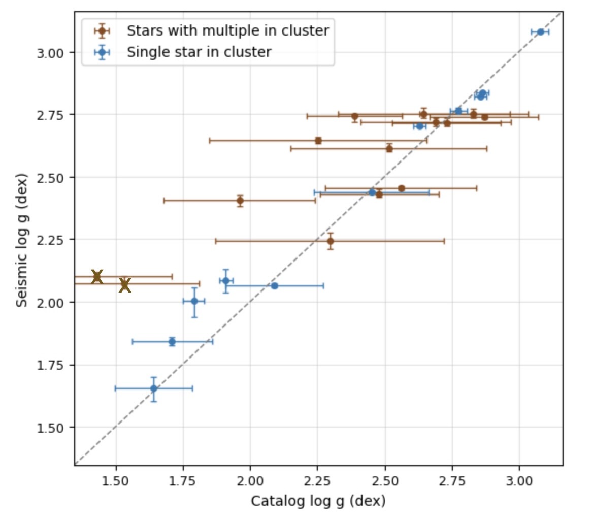
We validate surface gravity estimates by comparing spectroscopic $\log g$ with values inferred seismically via the $\nu_{\max}$ scaling relation, plotting $\log g_{\rm spec}$ against $\log g_{\rm seis}$ with uncertainties and a $1{:}1$ reference line. On the full set ( $N=25$ ), we find a bias of $+0.108\,\mathrm{dex}$ , median offset $+0.015\,\mathrm{dex}$ , $\mathrm{RMSE}=0.236\,\mathrm{dex}$ , robust spread $1.4826\times\mathrm{MAD}=0.124\,\mathrm{dex}$ , and $R^{2}=0.744$ , where $\mathrm{MAD}$ is the median absolute deviation. After removing two outliers using a MAD- $z$ cut (with MAD- $z$ defined as the absolute deviation from the median divided by $1.4826\times\mathrm{MAD}$ ), the remaining $N=23$ stars yield a bias of $+0.065\,\mathrm{dex}$ , median offset $-0.000\,\mathrm{dex}$ , $\mathrm{RMSE}=0.167\,\mathrm{dex}$ , robust spread $1.4826\times\mathrm{MAD}=0.112\,\mathrm{dex}$ , and $R^{2}=0.828$ , indicating consistency between spectroscopic and seismic $\log g$ .

III.4 Radius Comparison

Using the method outlined in §II.10, stellar radii are compared between seismic scaling-relation estimates and Gaia-based determinations. For each star, we use $\Delta\nu$ , $\nu_{\max}$ , and $T_{\rm eff}$ to compute $R_{\rm seis}$ and compare these values against the FLAME $R_{\rm\textit{Gaia}}$ derived from Gaia parallaxes and bolometric corrections (Gaia Collaboration, 2022). We quantify the agreement using fractional differences and dispersion, and present scatter plots with $1{:}1$ reference lines to assess systematic offsets. On the full member set ( $N=13$ ), we find a bias of $+0.396\,R_{\odot}$ , median offset $+0.165\,R_{\odot}$ , $\mathrm{RMSE}=5.165\,R_{\odot}$ , robust spread $1.4826\times\mathrm{MAD}=0.709\,R_{\odot}$ , and $R^{2}=-0.132$ . After removing four outliers with a MAD- $z$ cut, the remaining $N=9$ targets yield a bias of $+0.082\,R_{\odot}$ , median offset $+0.005\,R_{\odot}$ , $\mathrm{RMSE}=0.428\,R_{\odot}$ , robust spread $1.4826\times\mathrm{MAD}=0.469\,R_{\odot}$ , and $R^{2}=0.992$ , indicating consistency between seismic and Gaia-based radii and validating our choice to use $f_{\nu_{\max}}$ = 1.

III.5 Mass Comparison

Using the method described in §II.11, we present the seismic masses for all clusters in our sample. We report on the internal coherence of each cluster’s mass distribution. In Figure 11, each cluster forms a generally tight cluster around a single mass. Each mass in our sample is derived independently from its own seismic observables and this type of coherence is expected for members of a coeval population.

III.6 Stellar Age Validation

As stated in §II.12, we adopt four independent sets of stellar-evolution models (YREC, Dartmouth/DSEP, GARSTEC, and MIST) and follow the multi-model strategy suggested by Pinsonneault et al. (2025). We use the dispersion among the four models to quantify the model-dependent component of the age uncertainty. For red clump stars, we assume no mass loss in the models when estimating ages, so the inferred ages correspond to stars that retain their initial masses, a reasonable limiting case for young clusters where mass loss is expected to be small (Pinsonneault et al., 2025).

Although our stars reside in clusters, not all of these clusters have a single well-determined age in the literature. For the 12 clusters with seismically inferred ages in this work, we compile the published ages and their spread in Table 2. Our model-based cluster ages are then compared to the mean literature ages, with error bars reflecting the literature scatter, in Figure 12. For all clusters, Figure 13 shows the distribution of stellar ages within each cluster relative to the corresponding literature value. In general, our results are consistent with literature values, although in some cases, our data show a preference for one group of ages over another. The level of internal consistency indicates that the method yields reliable cluster ages and supports its use as a basis for deriving ages of stars outside of clusters, where such calibrated seismic ages are particularly valuable for galactic-archaeology applications.

Table 1: Compiled ages of the star clusters.

Cluster	Number of lit. age sources	Mean lit. age (Gyr)	Cantat-Gaudin (2020) age (Gyr)	Hunt & Reffert (2023) age (Gyr)	Seismic age (Gyr)
IC 348	8	0.005 $\pm$ 0.003	0.012	0.006	1.189 $\pm$ 0.309
Unknown 1	0	–	–	–	0.734 $\pm$ 0.280
Unknown 2	0	–	–	–	0.221 $\pm$ 0.237
LISC_3534	1	0.149	–	0.149	0.118 $\pm$ 0.752
COIN-Gaia_30	2	0.206 $\pm$ 0.052	0.257	0.154	4.251 $\pm$ 3.274
UPK 287	2	0.222 $\pm$ 0.060	0.257	0.154	0.667 $\pm$ 0.146
HSC_1052	1	0.068	0.068	–	0.108 $\pm$ 0.059
Unknown 3	0	–	–	–	6.405 $\pm$ 2.643
UPK 237	2	0.103 $\pm$ 0.048	0.151	0.055	0.262 $\pm$ 0.124
Casado Alessi-1	4	1.111 $\pm$ 0.337	1.445	0.749	1.706 $\pm$ 0.583
NGC 752	4	1.299 $\pm$ 0.166	1.175	1.421	1.433 $\pm$ 0.366
Theia 6046	1	3.807	–	3.807	0.525 $\pm$ 0.082

References: (1) Strom et al. (1974); (2) Herbig (1998); (3) Trullols and Jordi (1997); (4) Haisch et al. (2001); (5) Lada et al. (2006); (6) Luhman (1999); (7) Nikoghosyan et al. (2015); (10) Hunt and Reffert (2023b); (12) Carrera et al. (2019); (13) Sarajedini (2009); (14) Barnes et al. (2016); (15) Geller et al. (2021); (16) Carraro et al. (1994); (17) Hassan (1972); (18) Peña and Peniche (1994); (19) Maitzen and Hensberge (1981); (20) Reyes et al. (2025)

III.6.1 Casado Alessi-1

As shown in Figure 13, the interpolated ages for members of Casado Alessi-1 are not fully consistent with the literature range presented in past works. We were able to locate four age estimates for the cluster, 0.78, 0.8, 1.445, and 1.45 Gyr. Across our three estimations, the mean ages for Casado Alessi-1 are $1.63$ , $1.94$ , and $1.55$ Gyr; in each case, the quoted $1\sigma$ error bars extend down into the 0.8–1.45 Gyr literature range, but the central values remain systematically higher. To explore this tension, we plot MIST isochrones of various ages on top of our catalog members of Casado Alessi-1, removing any targets that are outside of a $2\sigma$ window in parallax and proper motion around the adopted cluster means (or with $\mathrm{RUWE}>1.4$ ) and may not be actual cluster members (Figure 14(c)). A discrepancy may arise from different membership selections or fitting choices in past or current work. Given our seismic uncertainties (Table 2) and analysis of isochrones compared to the cluster as a whole, we suspect that the age of this cluster may have been previously underestimated, but more detailed study is likely needed to solidify this age. We include Table 2 specifically to demonstrate that large per-star age uncertainties and grid-to-grid differences are common which makes the prevalence of error in cluster age determinations explicit. The full isochrone-fitting workflow for Casado Alessi-1 is available on GitHub.

Table 2: Ages and model comparisons for three Casado Alessi-1 giants.

TICID	age_gyr	age_std	age_gyr_ $-$ 1 $\sigma$	age_gyr_ $+$ 1 $\sigma$	age_MIST	age_Dartmouth	age_GARSTEC	age_YREC
306552813	1.627	0.811	2.254	1.127	1.843	2.746	2.469	2.299
306955660	1.944	0.905	2.748	1.261	2.169	2.950	2.479	2.301
306187638	1.547	0.780	2.203	1.150	1.764	2.689	2.465	2.297

III.6.2 NGC 752

As shown in Figure 13, the interpolated ages for members of NGC 752 are broadly consistent with the literature range reported in past work. Published ages for this nearby open cluster fall in the 1.3–1.6 Gyr range (Cantat-Gaudin and Anders, 2020; Hunt and Reffert, 2023a). Our seismically derived ages for NGC 752 lie within this interval; in each case, the quoted $1\sigma$ error bars overlap the canonical literature range and the central values do not show any strong offset.

To further assess this agreement, we repeat the isochrone-based test used for Casado Alessi-1. In Figure 14(a) we plot Gaia DR3 color–magnitude data for likely members of NGC 752, removing stars that lie outside a $2\sigma$ window in parallax and proper motion around the adopted cluster means (or with $\mathrm{RUWE}>1.4$ ), and marking the rejected targets with red crosses. We overplot MIST isochrones with ages of 1.30, 1.40, 1.50, and 1.60 Gyr. The 1.3–1.5 Gyr isochrones provide a visibly good match to the main sequence, turnoff, and base of the red giant branch, reinforcing the conclusion that our seismic ages for NGC 752 are consistent with the literature values. The full isochrone-fitting workflow for NGC 752 is available on GitHub.

III.6.3 Theia 6046

As shown in Figure 13, the interpolated ages for members of Theia 6046 differ from the value reported in large catalog work. Hunt & Reffert (2023a) give a cluster age of $\log t\approx 9.58$ (roughly $3.8$ Gyr), whereas our seismic estimation yields ages on the order of $\sim$ Gyr, substantially younger than this catalog value.

To explore this discrepancy, we repeat the isochrone-based test used for Casado Alessi-1 and NGC 752. In Figure 14(b) we plot Gaia DR3 color–magnitude data for likely members of Theia 6046, removing stars that lie outside a $2\sigma$ window in parallax and proper motion around the adopted cluster means (or with $\mathrm{RUWE}>1.4$ ), and marking the rejected targets with red crosses. We overplot MIST isochrones with ages of 0.3, 0.5, 0.7, 1.0, 1.5, and 3.7 Gyr. The younger ( $\lesssim 1$ Gyr) isochrones provide a visibly better match to the main sequence and turnoff than the older $\sim 3.7$ Gyr track, suggesting that the true cluster age is likely younger than the catalog value. As with Casado Alessi-1, details of the membership selection and fitting methodology likely contribute to the discrepancy, but more detailed study is likely needed to solidify this age. The full isochrone-fitting workflow for Theia 6046 is available on GitHub.

IV Conclusion and Future Work

We conclude that our method expands the available targets for asteroseismic analysis in star clusters using TESS light curves. We assembled a cluster-star catalog and workflow that integrates Gaia astrometry with TESS photometry to present red giants in clusters that are suitable for asteroseismic analysis. Our method (i) enforces distance, magnitude, and crowding/bleeding quality cuts, (ii) retrieves and preprocesses light curves, (iii) measures $\nu_{\max}$ and $\Delta\nu$ using PySYD, (iv) applies community and model-based corrections, (v) propagates uncertainties, (vi) validates radii, masses, and surface gravities across independent diagnostics, and (vii) compares our ages inferred from the asteroseismic analysis of red giants to the ages inferred in the literature from cluster CMDs. Our resulting catalogs, tables, cutouts, and notebooks provide a framework for expanding asteroseismology in clusters.

Our methodology is generally consistent with clusters having homogeneous ages. We show in Figure 12 that our independent ages for each star in the cluster are consistent in a way that allows us to combine estimates and infer cluster ages to a high degree of precision. We also show in Figure 13 that our ages are generally consistent with the literature ages for our clusters. We show in Figure 14 that, across NGC 752, Casado Alessi-1, and Theia 6046, the CMD-based isochrone fits can favor the catalog ages, the seismic ages, or strongly contradict the older catalog value in favor of a younger seismic solution. More generally, this suggests that asteroseismology can be a competitive way to infer cluster age, but that in many cases more detailed analysis of each cluster can be used to improve age estimates (Reyes et al., 2025). We view this paper primarily as a demonstration of the possibility of using TESS, even with its large pixel size and other limitations, to infer reliable cluster ages. We also hope that this analysis can serve as an initial step towards more detailed analysis of both individual stars and clusters in asteroseismic studies. We expect that additional spectroscopy (Otto et al., 2025), more advanced light-curve processing techniques (Pope et al., 2016), and individual mode analyses in clusters (Lindsay et al., 2025) would further tighten the constraints reported here. More generally, our work is intended as a contribution to a longer-term, community-wide effort to obtain robust asteroseismic mass and age estimates by combining stellar-evolution models and isochrones, detailed mode-by-mode asteroseismic analysis, comparisons to eclipsing binaries with dynamical masses, and the use of wide binaries and star clusters as coeval benchmarks (El-Badry et al., 2021; Godoy-Rivera and Chanamé, 2018; Tayar and Joyce, 2025; Theodoridis et al., 2025). Within this broader framework, the cluster-calibrated ages presented here help to cement asteroseismology as a precise and accurate technique for interpreting both exoplanetary systems and large galactic-archaeology samples such as APOGEE.

Clusters have long been our benchmarks for inferring stellar ages and calibrating other techniques. Our results suggest that ages inferred from asteroseismology can be reliable in clusters, and that more clusters are available to enhance calibration efforts. Looking ahead, space missions such as ESA’s PLATO (Rauer et al., 2014) and NASA’s Roman Space Telescope (Troxel et al., 2021) will offer the possibility of precise ages for hundreds of thousands of targets and extend this approach to even larger distances. To make full use of the precision of asteroseismology on such a broad scale, it is necessary to validate its accuracy against key calibration systems such as star clusters and wide binaries, and to compare it with other techniques over a range of ages and metallicities (Miglio et al., 2013, 2021b). Using tools like Roman, PLATO, and other dedicated missions (Miglio et al., 2021a) in this way will allow us to unlock the detailed evolutionary history of the Milky Way in a fully multidimensional sense.

Acknowledgments

This work was supported by the University of Florida College of Liberal Arts and Sciences. C. Mankowski received course credit for this research through the Department of Astronomy. We thank J. Tayar for supervision and weekly discussions guiding the analysis. We acknowledge helpful assistance with PySYD from A. Beyer. We thank D. Stello, N. Myers, M. Howell, Y. Noureddine, and C. Wagner for careful reading of the manuscript and for constructive feedback that improved this work. This paper includes data collected by the TESS mission and obtained from the Mikulski Archive for Space Telescopes (MAST) at the Space Telescope Science Institute (STScI). The TESS mission is funded by NASA’s Science Mission Directorate, and funding for TESS is provided by the NASA Explorer Program. STScI is operated by the Association of Universities for Research in Astronomy, Inc., under NASA contract NAS 5–26555. Some of the data presented in this paper were obtained from MAST. Support for MAST for non-HST data is provided by the NASA Office of Space Science via grant NAG5-7584 and by other grants and contracts.

This work has made use of data from the European Space Agency (ESA) mission Gaia (https://www.cosmos.esa.int/gaia), processed by the Gaia Data Processing and Analysis Consortium (DPAC, https://www.cosmos.esa.int/web/gaia/dpac/consortium). Funding for the DPAC has been provided by national institutions, in particular the institutions participating in the Gaia Multilateral Agreement.

Author Contributions

C. Mankowski carried out all aspects of this project, including data compilation, target selection, light curve analysis, seismic parameter extraction, application of corrections, age fitting, figure generation, and manuscript preparation, with the exception of Section 2.5 of the Methods, which was written and performed by C. Martin. J. Tayar conceived the project through her original proposal, provided overall supervision, provided manuscript edits, and met with C. Mankowski weekly to discuss methodology, results, and interpretation.

Software and third party data repository citations

This research made use of astropy (Astropy Collaboration et al., 2013, 2018, 2022), lightkurve (Lightkurve Collaboration, 2018), PySYD (Chontos et al., 2022a), asfgrid (Sharma et al., 2016), MIST (Choi et al., 2016), Dartmouth (Dotter et al., 2008), YREC (Demarque et al., 2008), GARSTEC (Weiss and Schlattl, 2008), and visualization and analysis packages including numpy, pandas, scipy, matplotlib, Échelle (Hey and Ball, 2020a), Bokeh (Bokeh Development Team, 2018), Panel, astroquery, and ebf. This work was partially carried out in the TIKE (Timeseries Integrated Knowledge Engine) environment provided by STScI/MAST.

We made use of data from the Mikulski Archive for Space Telescopes (MAST) for TESS observations, the ESA Gaia Archive for DR3 data.

References

R. Andrae, H. Rix, and V. Chandra (2023) Robust data-driven metallicities for 175 million stars from gaia xp spectra. The Astrophysical Journal Supplement Series 267 (1), pp. 8. External Links: Document Cited by: §II.4, §II.9.
A. L. Ash, M. H. Pinsonneault, M. Vrard, and J. Zinn (2024) Testing the breakdown of the asteroseismic scaling relations in luminous red giants. arXiv e-prints. External Links: 2411.10520, Link Cited by: §I.
Astropy Collaboration, A. M. Price-Whelan, P. L. Lim, et al. (2022) The astropy project: sustaining and growing a community-oriented open-source project and the v5.0 core package. The Astrophysical Journal 935 (2), pp. 167. External Links: Document Cited by: Software and third party data repository citations.
Astropy Collaboration, A. M. Price-Whelan, B. M. Sipőcz, et al. (2018) The astropy project: building an open-science project and status of the v2.0 core package. The Astronomical Journal 156 (3), pp. 123. External Links: Document Cited by: Software and third party data repository citations.
Astropy Collaboration, T. P. Robitaille, E. J. Tollerud, P. Greenfield, M. Droettboom, et al. (2013) Astropy: a community python package for astronomy. Astronomy & Astrophysics 558, pp. A33. External Links: Document Cited by: Software and third party data repository citations.
A. Baglin, M. Auvergne, P. Barge, et al. (2006) CoRoT: description of the mission and early results. The Publications of the Astronomical Society of the Pacific 118 (848), pp. 140–150. External Links: Document Cited by: §I.
T. Barclay, C. J. Burke, J. Catanzarite, D. Huber, C. Hedges, F. Mullally, J. Rowe, E. V. Quintana, and J. K. Zink (2020) Revised tess full frame image light curves: a uniform search for transiting exoplanets and variable stars. arXiv e-prints. External Links: 2002.01502, Link Cited by: §I.
S. A. Barnes, J. Weingrill, D. Fritzewski, K. G. Strassmeier, and I. Platais (2016) Rotation Periods for Cool Stars in the 4 Gyr old Open Cluster M67, The Solar-Stellar Connection, and the Applicability of Gyrochronology to at least Solar Age. ApJ 823 (1), pp. 16. External Links: Document, 1603.09179 Cited by: Table 1.
T. R. Bedding and H. Kjeldsen (2022) Dealing with large gaps in asteroseismic time series. Research Notes of the American Astronomical Society 6 (9), pp. 199. External Links: Document Cited by: §II.6.
Bokeh Development Team (2018) Bokeh: interactive data visualization in python. Note: Astrophysics Source Code Libraryascl:1806.014 Cited by: Software and third party data repository citations.
W. J. Borucki, D. Koch, G. Basri, N. Batalha, T. M. Brown, S. T. Bryson, D. Caldwell, J. Christensen-Dalsgaard, W. D. Cochran, E. DeVore, E. W. Dunham, T. N. Gautier, J. C. Geary, R. Gilliland, A. Gould, S. B. Howell, J. M. Jenkins, D. W. Latham, J. J. Lissauer, G. W. Marcy, J. Rowe, D. Sasselov, A. Boss, D. Charbonneau, D. Ciardi, L. Doyle, A. K. Dupree, E. B. Ford, J. Fortney, M. J. Holman, S. Seager, J. H. Steffen, J. Tarter, W. F. Welsh, C. Allen, L. A. Buchhave, J. L. Christiansen, B. D. Clarke, S. Das, J. Désert, M. Endl, D. Fabrycky, F. Fressin, M. Haas, E. Horch, A. Howard, H. Isaacson, H. Kjeldsen, J. Kolodziejczak, C. Kulesa, J. Li, P. W. Lucas, P. Machalek, D. McCarthy, P. MacQueen, S. Meibom, T. Miquel, A. Prša, S. N. Quinn, E. V. Quintana, D. Ragozzine, W. Sherry, A. Shporer, P. Tenenbaum, G. Torres, J. D. Twicken, J. Van Cleve, L. Walkowicz, F. C. Witteborn, and M. Still (2010) Kepler planet-detection mission: introduction and first results. Science 327 (5968), pp. 977–980. External Links: Document Cited by: §I.
A. W. Boyle, A. W. Mann, and J. Bush (2025) Quantifying the limits of tess stellar rotation measurements with the k2–tess overlap. The Astrophysical Journal 985 (2), pp. 233. External Links: Document, Link Cited by: §II.3.
T. M. Brown, J. Christensen-Dalsgaard, W. A. Dziembowski, P. R. Goode, D. O. Gough, and C. A. Morrow (1989) Inferring the sun’s internal angular velocity from observed p-mode splittings. The Astrophysical Journal 343, pp. 526–531. Cited by: §I.
S. Buder, S. Sharma, J. Kos, A. M. Amarsi, T. Nordlander, M. R. Hayden, M. Asplund, J. Bland-Hawthorn, A. R. Casey, G. M. De Silva, K. C. Freeman, J. Lin, D. B. Zucker, T. Zwitter, and et al. (2021) The galah+ survey: third data release. Monthly Notices of the Royal Astronomical Society 506, pp. 150–201. External Links: Document Cited by: §I.
T. Cantat-Gaudin and F. Anders (2020) Clusters and mirages: cataloguing stellar aggregates in the milky way. Astronomy & Astrophysics 633, pp. A99. External Links: Document Cited by: §I, §II.1, §II.1, §II.2, Figure 14, Figure 14, §III.1.1, §III.6.2.
G. Carraro, C. Chiosi, A. Bressan, and G. Bertelli (1994) Five old open clusters: NGC 2682, NGC 2243, Berkeley 39, NGC 188 and NGC 6791. A&AS 103, pp. 375–389. Cited by: Table 1.
R. Carrera, M. Pasquato, A. Vallenari, L. Balaguer-Núñez, T. Cantat-Gaudin, M. Mapelli, A. Bragaglia, D. Bossini, C. Jordi, D. Galadí-Enríquez, and E. Solano (2019) The extended halo of ngc 2682 (m 67) from gaia dr2. arXiv preprint arXiv:1905.02020. Note: Accepted for publication on A&A External Links: 1905.02020 Cited by: Table 1.
G. Casali, L. Magrini, G. Tautvaišienė, C. Viscasillas Vázquez, S. Feltzing, F. M. Jiménez-Esteban, S. Randich, A. Bragaglia, and et al. (2022) The gaia-eso survey: calibrating age-chemical clock relations across the galactic disc. Astronomy & Astrophysics 666, pp. A180. External Links: Document Cited by: §I.
W. J. Chaplin and A. Miglio (2013) Asteroseismology of solar-type and red-giant stars. Annual Review of Astronomy and Astrophysics 51, pp. 353–392. External Links: Document Cited by: §I.
J. Choi, A. Dotter, C. Conroy, M. Cantiello, B. Paxton, and B. D. Johnson (2016) MESA isochrones and stellar tracks (mist). i. solar-scaled models. The Astrophysical Journal 823 (2), pp. 102. External Links: Document Cited by: §II.12, Software and third party data repository citations.
A. Chontos, D. Huber, A. Beyer, et al. (2022a) PySYD: python implementation of the syd asteroseismic pipeline. Note: https://github.com/ashleychontos/pysyd Cited by: Software and third party data repository citations.
A. Chontos, D. Huber, M. Sayeed, and P. Yamsiri (2022b) PySYD: automated measurements of global asteroseismic parameters. Journal of Open Source Software 7 (79), pp. 3331. External Links: Document Cited by: §II.6, §II.9.
Z. R. Claytor, J. L. van Saders, Á. R. G. Santos, R. A. García, S. Mathur, J. Tayar, M. H. Pinsonneault, and M. Shetrone (2020) Chemical evolution in the milky way: rotation-based ages for apogee-Kepler cool dwarf stars. The Astrophysical Journal 888, pp. 43. External Links: Document Cited by: §II.12.
Z. R. Claytor (2020) Kiauhoku: stellar model grid interpolation Note: Astrophysics Source Code Library, ascl:2011.027 External Links: Link Cited by: §II.12.
P. Demarque, D. B. Guenther, L. Li, A. Mazumdar, and C. W. Straka (2008) YREC: the yale rotating stellar evolution code. Astrophysics and Space Science 316, pp. 31–41. External Links: Document Cited by: Software and third party data repository citations.
A. Dotter, B. Chaboyer, D. Jevremović, E. Baron, J. W. Ferguson, A. Sarajedini, and J. Anderson (2008) The dartmouth stellar evolution database. The Astrophysical Journal Supplement Series 178 (1), pp. 89–101. External Links: Document Cited by: §II.12, Software and third party data repository citations.
P. D. Edmonds and R. L. Gilliland (1996) Hubble Space Telescope Time-Series Photometry of the Pre-Cataclysmic Variable PG 1336-018. ApJ 470, pp. L85. External Links: astro-ph/9608067, Document Cited by: §I.
K. El-Badry, H. Rix, and T. M. Heintz (2021) A million binaries from Gaia edr3: sample selection and validation of Gaia parallax uncertainties. Monthly Notices of the Royal Astronomical Society 506 (2), pp. 2269–2295. External Links: Document Cited by: §IV.
Y. Elsworth, S. Hekker, J. A. Johnson, T. Kallinger, B. Mosser, M. Pinsonneault, M. Hon, J. Kuszlewicz, A. Miglio, A. Serenelli, D. Stello, J. Tayar, and M. Vrard (2019) Insights from the apokasc determination of the evolutionary state of red-giant stars by consolidation of different methods. Monthly Notices of the Royal Astronomical Society 489 (4), pp. 4641–4657. External Links: Document Cited by: §II.9.
M. Fausnaugh and the TESS Team (2023) TESS data release notes: sector 59, dr84. Technical report Technical Report DR84, TESS Science Office. Note: Accessed 2025-10-19 External Links: Link Cited by: §II.3.
D. K. Feuillet, J. Bovy, J. Holtzman, D. H. Weinberg, D. A. García-Hernández, F. R. Hearty, S. R. Majewski, A. Roman-Lopes, J. Rybizki, and O. Zamora (2018) Age-resolved chemistry of red giants in the solar neighbourhood. Monthly Notices of the Royal Astronomical Society 477 (2), pp. 2326–2348. External Links: Document Cited by: §I.
M. Gai, A. Vecchiato, A. Riva, D. Busonero, M. Lattanzi, B. Bucciarelli, M. Crosta, and Z. Qi (2022) Astrometric precision tests on tess data. arXiv e-prints. External Links: 2212.02357 Cited by: §II.1.
Gaia Collaboration, C. Babusiaux, F. van Leeuwen, et al. (2018) Gaia data release 2: observational hertzsprung–russell diagrams. Astronomy & Astrophysics 616, pp. A10. External Links: Document Cited by: §II.4, §II.9.
Gaia Collaboration, A. G. A. Brown, A. Vallenari, T. Prusti, J. H. J. de Bruijne, C. Babusiaux, M. Biermann, O. L. Creevey, D. W. Evans, L. Eyer, A. Hutton, F. Jansen, C. Jordi, S. A. Klioner, U. Lammers, L. Lindegren, X. Luri, F. Mignard, C. Panem, D. Pourbaix, S. Randich, P. Sartoretti, C. Soubiran, N. A. Walton, and et al. (2023) Gaia data release 3: summary of the contents and survey properties. Astronomy & Astrophysics 674, pp. A1. External Links: Document Cited by: §II.1.
Gaia Collaboration (2022) Gaia dr3 astrophysical parameters supplement: flame results. Note: Gaia DPAC documentation, Astrophysical Parameters Supplement (gaiadr3.astrophysical_parameters_supp)https://doi.org/10.17876/gaia/dr.3/44 Cited by: §II.13.2, §II.9, §III.4.
A. M. Geller, R. D. Mathieu, D. W. Latham, M. Pollack, G. Torres, and E. M. Leiner (2021) Stellar Radial Velocities in the Old Open Cluster M67 (NGC 2682). II. The Spectroscopic Binary Population. AJ 161 (4), pp. 190. External Links: Document, 2101.07883 Cited by: Table 1.
D. Godoy-Rivera and J. Chanamé (2018) On the identification of wide binaries in the Kepler field. Monthly Notices of the Royal Astronomical Society 479 (4), pp. 4440–4458. External Links: Document Cited by: §IV.
S. Grusnis, J. Tayar, and D. Godoy-Rivera (2025) TESS subgiant and lower red giant asteroseismology in the continuous viewing zones. arXiv e-prints. External Links: 2509.12513 Cited by: §II.3, §II.9.
N. M. Guerrero et al. (2021) The tess objects of interest catalog from the tess prime mission. The Astrophysical Journal Supplement Series 254, pp. 39. Cited by: §I.
K. E. Haisch, E. A. Lada, and C. J. Lada (2001) Circumstellar Disks in the IC 348 Cluster. AJ 121 (4), pp. 2065–2074. External Links: Document, astro-ph/0101486 Cited by: Table 1.
S. M. Hassan (1972) A new photometric investigation of NGC 1662.. Mem. Soc. Astron. Italiana 43, pp. 117–122. Cited by: Table 1.
E. Hatt, M. B. Nielsen, W. J. Chaplin, W. H. Ball, G. R. Davies, T. R. Bedding, D. L. Buzasi, A. Chontos, D. Huber, C. Kayhan, Y. Li, T. R. White, C. Cheng, T. S. Metcalfe, and D. Stello (2023) A catalogue of solar-like oscillators observed by tess in 120-second and 20-second cadence. Astronomy & Astrophysics 669, pp. A67. External Links: Document Cited by: §I.
S. Hekker, R. L. Gilliland, Y. Elsworth, W. J. Chaplin, J. De Ridder, D. Stello, T. Kallinger, K. A. Ibrahim, T. C. Klaus, and J. Li (2011) Solar-like oscillations in cluster red giants observed during campaign 1 of the kepler k2 mission. Monthly Notices of the Royal Astronomical Society 414 (3), pp. 2594–2603. External Links: Document Cited by: §I.
G. H. Herbig (1998) The Young Cluster IC 348. ApJ 497 (2), pp. 736–758. External Links: Document Cited by: Table 1.
D. Hey and W. H. Ball (2020a) Echelle: Échelle diagrams for asteroseismology. Journal of Open Source Software 5 (46), pp. 2051. External Links: Document Cited by: Software and third party data repository citations.
D. Hey and W. Ball (2020b) Echelle: Dynamic echelle diagrams for asteroseismology External Links: Document, Link Cited by: §II.8.
M. Hon, D. Huber, J. S. Kuszlewicz, D. Stello, S. Sharma, J. Tayar, J. C. Zinn, M. Vrard, and M. H. Pinsonneault (2021) A “quick look” at all-sky galactic archeology with tess: 158,000 oscillating red giants from the mit quick-look pipeline. The Astrophysical Journal 919 (2), pp. 131. External Links: ISSN 1538-4357, Link, Document Cited by: §I, §II.3, §II.4.
M. Hon, J. Yu, D. Huber, W. R. Wolf, W. J. Chaplin, D. Stello, W. H. Ball, B. Mosser, E. Corsaro, and H. Kjeldsen (2024) Asteroseismology of the nearby k-dwarf $\sigma$ draconis using the keck planet finder and tess. arXiv e-prints. External Links: 2407.21234 Cited by: §I, §I, §II.7.
D. Horta, Y. Lu, M. K. Ness, M. Lisanti, and A. M. Price-Whelan (2024) Stellar mergers or truly young? intermediate-age stars on highly radial orbits in the milky way’s stellar halo. The Astrophysical Journal 971, pp. 170. External Links: Document Cited by: §I.
M. Howell, S. W. Campbell, C. Kalup, D. Stello, and G. M. De Silva (2024) Asteroseismic masses of red giants in the galactic globular clusters m9 and m19. Monthly Notices of the Royal Astronomical Society 536 (2), pp. 1389–1407. External Links: ISSN 0035-8711, Document, Link, https://academic.oup.com/mnras/article-pdf/536/2/1389/61181833/stae2686.pdf Cited by: §I.
S. B. Howell, C. Sobeck, M. Haas, M. Still, T. Barclay, F. Mullally, J. Troeltzsch, S. Aigrain, S. T. Bryson, D. Caldwell, W. J. Chaplin, W. D. Cochran, D. Huber, G. W. Marcy, A. Miglio, A. J. Monson, M. Smith, J. D. Twicken, and J. J. Fortney (2014) The k2 mission: characterization and early results. Publications of the Astronomical Society of the Pacific 126 (938), pp. 398. External Links: Document Cited by: §I.
D. Huber et al. (2009) Automated extraction of oscillation parameters for kepler. Communications in Asteroseismology 160, pp. 74. External Links: Link Cited by: §II.7.
E. L. Hunt and S. Reffert (2023a) Improving the open cluster census. ii. an all-sky cluster catalogue with gaia dr3. Astronomy & Astrophysics 673, pp. A114. External Links: Document Cited by: §I, §II.1, §II.1, Figure 14, Figure 14, §III.1.1, §III.6.2, §III.6.3.
E. L. Hunt and S. Reffert (2023b) Improving the open cluster census. II. An all-sky cluster catalogue with Gaia DR3. A&A 673, pp. A114. External Links: Document, 2303.13424 Cited by: Table 1.
J. M. Jenkins, J. D. Twicken, S. McCauliff, et al. (2016) The tess science processing operations center. Proceedings of the SPIE 9913, pp. 99133E. External Links: Document Cited by: §I, §II.6.
H. Kjeldsen and T. R. Bedding (1995) Amplitudes of stellar oscillations: the implications for asteroseismology. Astronomy and Astrophysics 293, pp. 87–106. External Links: astro-ph/9403015, Link Cited by: §I.
T. Konchady (2020) Getting deeper into the main sequence with Gaia. Note: AAS Nova External Links: Link Cited by: §II.4.
C. J. Lada, A. A. Muench, K. L. Luhman, L. Allen, L. Hartmann, T. Megeath, P. Myers, G. Fazio, K. Wood, J. Muzerolle, G. Rieke, N. Siegler, and E. Young (2006) Spitzer Observations of IC 348: The Disk Population at 2-3 Million Years. AJ 131 (3), pp. 1574–1607. External Links: Document, astro-ph/0511638 Cited by: Table 1.
Y. Lebreton and J. Montalbán (2008) Stellar ages from asteroseismology. Proceedings of the International Astronomical Union 4 (S258), pp. 419–430. External Links: Document Cited by: §I.
Lightkurve Collaboration (2018) Lightkurve: kepler and tess time series analysis in python. Note: https://docs.lightkurve.orgAstrophysics Source Code Library, ascl:1812.013 Cited by: Software and third party data repository citations.
L. Lindegren et al. (2018) Gaia data release 2: the astrometric solution. Astronomy & Astrophysics 616, pp. A2. External Links: Document Cited by: §II.2.
C. J. Lindsay, M. Hon, J. M. J. Ong, R. A. García, D. B. Palakkatharappil, J. Yu, T. Li, T. Ruiz-Lara, and A. Helmi (2025) Precise asteroseismic ages for the helmi streams. The Astrophysical Journal. Note: accepted External Links: 2507.01091 Cited by: §II.9, §IV.
Y. Lu, R. Angus, M. A. Agüeros, et al. (2020) Astraea: predicting long rotation periods with 27-day light curves. The Astronomical Journal 160 (5), pp. 207. External Links: Document Cited by: §I.
K. L. Luhman (1999) Young Low-Mass Stars and Brown Dwarfs in IC 348. ApJ 525 (1), pp. 466–481. External Links: Document, astro-ph/9905287 Cited by: Table 1.
H. M. Maitzen and H. Hensberge (1981) A photoelectric investigation of Ap-stars in open clusters. I. NGC 2516 and NGC 1662.. A&A 96, pp. 151–157. Cited by: Table 1.
C. Marasco, J. Tayar, and D. Nidever (2025) Asteroseismology of metal-poor red giants observed by tess. The Astrophysical Journal 986, pp. 144. Cited by: §II.9.
A. Miglio, C. Chiappini, T. Morel, et al. (2013) Galactic archaeology: mapping and dating stellar populations with asteroseismology of red-giant stars. Monthly Notices of the Royal Astronomical Society 429, pp. 423–428. External Links: Document Cited by: §IV.
A. Miglio, C. Chiappini, B. Mosser, J. Montalbán, G. R. Davies, L. Girardi, S. Khan, B. M. Rendle, M. Valentini, L. Casagrande, A. Noels, F. Anders, T. S. Rodrigues, D. Bossini, M. H. Pinsonneault, J. Tayar, W. J. Chaplin, D. Kawata, I. Minchev, G. Buldgen, Y. Elsworth, N. Lagarde, S. J. A. J. Salmon, and E. Willett (2021a) Milky way seismology from tess and gaia synergy. Astronomy & Astrophysics 645, pp. A85. External Links: Document Cited by: §I, §I, §IV.
A. Miglio, L. Girardi, F. Grundahl, et al. (2021b) HAYDN: high-precision asteroseismology of dense stellar fields. Experimental Astronomy 51, pp. 963–1001. External Links: Document Cited by: §IV.
MIT TESS Science Office (2025) QLP – mit quick-look pipeline for tess ffis. Note: https://tess.mit.edu/qlp/QLP extracts FFI light curves for targets with TESS magnitude $T<13.5$ ; accessed 2025-10-19 Cited by: §II.3.
L. M. Morales, J. Tayar, and Z. R. Claytor (2025) Model choice matters for age inference on the red giant branch. The Astrophysical Journal 986 (2), pp. 229. External Links: Document, 2504.17600 Cited by: §II.12.
B. Mosser, Y. Elsworth, S. Hekker, D. Huber, T. Kallinger, S. Mathur, K. Belkacem, M. J. Goupil, R. Samadi, C. Barban, T. R. Bedding, W. J. Chaplin, R. A. Garcia, D. Stello, J. De Ridder, C. K. Middour, R. L. Morris, and E. V. Quintana (2012) Characterization of the power excess of solar-like oscillations in red giants with Kepler. Astronomy & Astrophysics 537, pp. A30. External Links: Document Cited by: §II.9.
B. Mosser, E. Michel, K. Belkacem, and R. Samadi (2018) Asteroseismology of red giants: observations with CoRoT and Kepler. In Handbook of Exoplanets, H. J. Deeg and J. A. Belmonte (Eds.), pp. 1–32. External Links: Document Cited by: §I.
S. J. Murphy (2015) The potential for super-nyquist asteroseismology with tess. Monthly Notices of the Royal Astronomical Society 453 (3), pp. 2569–2575. External Links: Document Cited by: §I.
N. Myers, J. Donor, T. Spoo, P. M. Frinchaboy, K. Cunha, A. M. Price-Whelan, S. R. Majewski, R. L. Beaton, G. Zasowski, J. O’Connell, A. E. Ray, D. Bizyaev, C. Chiappini, D. A. García-Hernández, D. Geisler, H. Jönsson, R. R. Lane, P. Longa-Peña, I. Minchev, D. Minniti, C. Nitschelm, and A. Roman-Lopes (2022) The open cluster chemical abundances and mapping survey. vi. galactic chemical gradient analysis from apogee dr17. The Astronomical Journal 164 (3), pp. 85. External Links: ISSN 1538-3881, Link, Document Cited by: §I.
E. H. Nikoghosyan, A. V. Vardanyan, and K. G. Khachatryan (2015) Statistical Analysis of Stars with H $\alpha$ Emission in the Cluster IC 348. Astrophysics 58 (4), pp. 490–502. External Links: Document, 1504.01156 Cited by: Table 1.
J. M. Otto, P. M. Frinchaboy, N. R. Myers, K. Cunha, J. W. Johnson, A. Hossain, G. Zasowski, S. Loebman, J. Donor, A. I. Wiggins, B. Bhattarai, S. Mészáros, T. Spoo, and A. M. Price-Whelan (2025) The open cluster chemical abundances and mapping survey: viii. galactic chemical gradient and azimuthal analysis from sdss-v/mwm dr19. The Astronomical Journal. Note: submitted External Links: 2507.07264 Cited by: §IV.
D. B. Palakkatharappil and O. L. Creevey (2023) Asteroseismic age constraints on the open cluster ngc 2477 using oscillating stars identified with tess ffi. Astronomy & Astrophysics 672, pp. A123. External Links: Document Cited by: §I.
J. H. Peña and R. Peniche (1994) uvby- $\beta$ photometry of open clusters. IV. NGC 1444, NGC 1662, NGC 2129, NGC 2169, and NGC 7209.. Rev. Mexicana Astron. Astrofis. 28, pp. 139–152. Cited by: Table 1.
M. H. Pinsonneault, J. C. Zinn, J. Tayar, A. Serenelli, R. A. García, S. Mathur, M. Vrard, Y. P. Elsworth, B. Mosser, D. Stello, K. J. Bell, L. Bugnet, E. Corsaro, P. Gaulme, S. Hekker, M. Hon, D. Huber, T. Kallinger, K. Cao, J. A. Johnson, B. Liagre, R. A. Patton, A. R. G. Santos, S. Basu, P. G. Beck, T. C. Beers, W. J. Chaplin, K. Cunha, P. M. Frinchaboy, L. Girardi, D. Godoy-Rivera, J. A. Holtzman, H. Jönsson, S. Mészáros, C. Reyes, H. Rix, M. Shetrone, V. V. Smith, T. Spoo, K. G. Stassun, and J. Wang (2025) APOKASC-3: the third joint spectroscopic and asteroseismic catalog for evolved stars in the kepler fields. The Astrophysical Journal Supplement Series 276 (2), pp. 69. External Links: Document Cited by: §II.12, §II.7, §II.8, §II.9, §II.9, §III.6.
B. J. S. Pope, T. R. White, D. Huber, S. J. Murphy, T. R. Bedding, D. A. Caldwell, A. Sarai, S. Aigrain, and T. Barclay (2016) Photometry of very bright stars with kepler and k2 smear data. Monthly Notices of the Royal Astronomical Society: Letters 455 (1), pp. L36–L40. External Links: Document, Link Cited by: §II.5, §IV.
H. Rauer, C. Catala, C. Aerts, T. Appourchaux, W. Benz, A. Brandeker, J. Christensen-Dalsgaard, et al. (2014) The plato 2.0 mission. Experimental Astronomy 38, pp. 249–330. External Links: Document Cited by: §IV.
C. Reyes, D. Stello, M. Hon, Y. Li, T. R. Bedding, E. Corsaro, L. Taylor, A. Vanderburg, E. Sandquist, and R. D. Mathieu (2025) Asteroseismic study of subgiants and giants of the open cluster m67 using kepler/k2: expanded sample and precise masses. Monthly Notices of the Royal Astronomical Society 538 (3), pp. 1720–1746. External Links: Document Cited by: §III.1.1, Table 1, §IV.
C. Reyes, D. Stello, M. Hon, R. Trampedach, E. Sandquist, and M. H. Pinsonneault (2024) Isochrone fitting of the open cluster m67 in the era of gaia and improved model physics. Monthly Notices of the Royal Astronomical Society 532 (2), pp. 2860–2874. External Links: ISSN 0035-8711, Document, Link, https://academic.oup.com/mnras/article-pdf/532/2/2860/58587176/stae1650.pdf Cited by: §I, Figure 6, Figure 6, Figure 7, Figure 7, §II.13.2.
G. R. Ricker, J. N. Winn, R. Vanderspek, D. W. Latham, G. Á. Bakos, J. L. Bean, Z. K. Berta-Thompson, T. M. Brown, L. A. Buchhave, N. R. Butler, J. L. Christiansen, M. Clampin, D. Deming, J. Doty, N. De Lee, C. Dressing, E. W. Dunham, M. Endl, F. Fressin, J. Ge, T. Henning, M. J. Holman, A. W. Howard, S. Ida, J. M. Jenkins, G. Jernigan, L. Kaltenegger, N. Kawai, H. Kjeldsen, G. Laughlin, A. M. Levine, D. Lin, J. J. Lissauer, P. MacQueen, G. Marcy, P. R. McCullough, T. D. Morton, N. Narita, M. Paegert, E. Pallé, F. Pepe, J. Pepper, A. Quirrenbach, S. A. Rinehart, D. Sasselov, B. Sato, S. Seager, A. Sozzetti, K. G. Stassun, P. Sullivan, G. Torres, S. Udry, and J. Villasenor (2015) Transiting exoplanet survey satellite (tess). Journal of Astronomical Telescopes, Instruments, and Systems 1 (1), pp. 014003. External Links: Document Cited by: §I, §I.
M. Riello, F. De Angeli, D. W. Evans, P. Montegriffo, J. M. Carrasco, G. Busso, L. Palaversa, P. W. Burgess, C. Diener, M. Davidson, N. Rowell, C. Fabricius, C. Jordi, M. Bellazzini, E. Pancino, D. L. Harrison, C. Cacciari, F. van Leeuwen, N. C. Hambly, S. T. Hodgkin, P. J. Osborne, G. Altavilla, M. A. Barstow, A. G. A. Brown, M. Castellani, S. Cowell, F. De Luise, G. Gilmore, G. Giuffrida, S. Hidalgo, G. Holland, S. Marinoni, C. Pagani, A. M. Piersimoni, L. Pulone, S. Ragaini, M. Rainer, P. J. Richards, N. Sanna, N. A. Walton, M. Weiler, and A. Yoldas (2021) Gaia early data release 3: photometric content and validation. Astronomy & Astrophysics 649, pp. A3. External Links: Document Cited by: §II.3.
S. Risbud, G. Carraro, and H. M. J. Boffin (2025) Tidal tails of nearby open clusters. i. mapping with gaia dr3. arXiv e-prints. External Links: 2501.17225, Link Cited by: §I.
L. Ruiz-Dern, C. Babusiaux, F. Arenou, C. Turon, and R. Lallement (2018) Empirical photometric calibration of the gaia red clump: colours, effective temperature, and absolute magnitude. Astronomy and Astrophysics 609, pp. A116. External Links: Document Cited by: §II.9.
A. Sarajedini (2009) Deep 2mass photometry of m67 and calibration of the main sequence j-ks color difference as an age indicator. arXiv preprint arXiv:0904.2907. Note: Astrophys.J.698:1872-1878,2009 External Links: 0904.2907 Cited by: Table 1.
R. Schiavon, S. Phillips, and D. Horta (2022) APOGEE detailed elemental abundances for thousands of globular cluster stars. The Value Added Catalogue.. In EAS2022, European Astronomical Society Annual Meeting, pp. 1681. Cited by: §II.1, §II.1.
A. M. Serenelli, M. Bergemann, G. Ruchti, and L. Casagrande (2013) Bayesian analysis of ages, masses and distances to cool stars with non-lte spectroscopic parameters. Monthly Notices of the Royal Astronomical Society 429 (4), pp. 3645–3657. External Links: Document Cited by: §II.12.
S. Sharma, D. Stello, J. Bland-Hawthorn, D. Huber, and T. R. Bedding (2016) Testing asteroseismic scaling relations using eclipsing binaries in the Kepler field. The Astrophysical Journal 822 (1), pp. 15. External Links: Document Cited by: §II.9, §II.9, Software and third party data repository citations.
S. Sharma, D. Stello, J. C. Zinn, C. Reyes, M. Hon, and J. Bland-Hawthorn (2022) The k2 galactic archaeology program: overview, target selection, and survey properties. Monthly Notices of the Royal Astronomical Society 517 (2), pp. 1970–1987. External Links: Document Cited by: §II.9.
K. G. Stassun, R. J. Oelkers, J. Pepper, and et al. (2019a) TESS input catalog version 7 (tic-7). Note: MAST—Mikulski Archive for Space TelescopesAccessible via MAST prior to the release of TIC-8 Cited by: §II.1.
K. G. Stassun, R. J. Oelkers, M. Paegert, G. Torres, J. Pepper, N. De Lee, K. I. Collins, D. W. Latham, P. S. Muirhead, J. S. Chittidi, B. Rojas-Ayala, S. W. Fleming, M. E. Rose, P. Tenenbaum, E. B. Ting, S. R. Kane, T. Barclay, J. L. Bean, C. E. Brassuer, D. Charbonneau, et al. (2019b) The revised tess input catalog and candidate target list. The Astronomical Journal 158 (4), pp. 138. External Links: Document Cited by: §II.3.
K. G. Stassun, R. J. Oelkers, M. Paegert, G. Torres, J. Pepper, N. De Lee, K. Collins, D. W. Latham, P. S. Muirhead, J. Chittidi, B. Rojas-Ayala, S. W. Fleming, M. E. Rose, P. Tenenbaum, E. B. Ting, S. R. Kane, T. Barclay, J. L. Bean, C. E. Brassuer, D. Charbonneau, J. J. Lissauer, A. W. Mann, B. McLean, S. Mulally, N. Narita, P. Plavchan, G. R. Ricker, D. Sasselov, S. Seager, S. Sharma, D. Stello, R. Vanderspek, G. Wallace, and J. N. Winn (2019c) TESS input catalog version 8.0 (tic-8). Note: VizieR Online Data CatalogReleased May 2019; uses Gaia DR2 base, contains 1̃.5 billion sources Cited by: §I, §II.1.
D. Stello and R. L. Gilliland (2009) Asteroseismology of Red Giants from the First Four Months of Kepler Data: Global Oscillation Parameters for 800 Stars. ApJ 700, pp. 1589. External Links: 0909.5194, Document Cited by: §I.
D. Stello and S. Sharma (2023) Extension of the asfgrid for correcting asteroseismic large frequency separations. External Links: 2305.03221, Link Cited by: §I, §II.9.
D. Stello, N. Saunders, S. Grunblatt, M. Hon, C. Reyes, D. Huber, T. R. Bedding, Y. Elsworth, R. A. García, S. Hekker, T. Kallinger, S. Mathur, B. Mosser, and M. H. Pinsonneault (2022) TESS asteroseismology of the kepler red giants. Monthly Notices of the Royal Astronomical Society 512 (2), pp. 1677–1686. External Links: ISSN 0035-8711, Document, Link, https://academic.oup.com/mnras/article-pdf/512/2/1677/42993204/stac414.pdf Cited by: §II.4.
S. E. Strom, K. M. Strom, and L. Carrasco (1974) A study of the young cluster IC 348.. PASP 86, pp. 798. External Links: Document Cited by: Table 1.
J. Tayar, Z. R. Claytor, D. Huber, and J. van Saders (2022) A guide to realistic uncertainties on the fundamental properties of solar-type exoplanet host stars. The Astrophysical Journal 927 (1), pp. 31. External Links: Document Cited by: §II.12.
J. Tayar and M. Joyce (2025) Star-crossed clusters: asteroseismic ages for individual stars are in tension with the ages of their host clusters. The Astrophysical Journal Letters 984 (L56). External Links: Document Cited by: §I, §I, §IV.
TESS Science Processing Operations Center (2025) TESS data release notes: sector 82 (drn-115). Technical report NASA Ames Research Center. Note: Accessed June 2025 External Links: Link Cited by: §II.3.
A. T. Theodoridis, L. Morales, and J. Tayar (2025) Asteroseismically inferred ages of 132,000 red giants with TESS. arXiv e-prints arXiv:2505.08109. External Links: Document, Link Cited by: §I, §I, §II.12, §IV.
D. Thomas, C. Maraston, R. Bender, and C. Mendes de Oliveira (2005) The epochs of early-type galaxy formation as a function of environment. The Astrophysical Journal 621 (2), pp. 673–694. External Links: Document Cited by: §I.
M. A. Troxel, H. Long, C. M. Hirata, A. Choi, M. Jarvis, R. Mandelbaum, K. Wang, M. Yamamoto, S. Hemmati, and P. Capak (2021) A synthetic roman space telescope high-latitude imaging survey: simulation suite and the impact of wavefront errors on weak gravitational lensing. Monthly Notices of the Royal Astronomical Society 501 (2). External Links: Document Cited by: §IV.
E. Trullols and C. Jordi (1997) Deep UBVRI photometry in IC 348.. A&A 324, pp. 549–555. Cited by: Table 1.
M. Tucci Maia, I. Ramírez, J. Meléndez, M. Bedell, J. L. Bean, and M. Asplund (2016) The solar twin planet search. iii. the [y/mg] clock: estimating stellar ages of solar-type stars. Astronomy & Astrophysics 590, pp. A32. External Links: Document, 1604.05733 Cited by: §I.
M. Vrard, M. H. Pinsonneault, Y. Elsworth, M. Hon, T. Kallinger, J. Kuszlewicz, B. Mosser, R. A. Garcia, J. Tayar, R. Bennett, K. Cao, S. Hekker, L. Loyer, S. Mathur, and D. Stello (2025) Red giant evolutionary status determination: the complete Kepler catalog. Astronomy & Astrophysics 697, pp. A165. External Links: Document Cited by: §II.9.
A. Weiss and H. Schlattl (2008) GARSTEC—the garching stellar evolution code. Astrophysics and Space Science 316, pp. 99–106. External Links: Document Cited by: §II.12, Software and third party data repository citations.
T. R. White, T. R. Bedding, D. Stello, J. Christensen-Dalsgaard, D. Huber, and H. Kjeldsen (2011) Calculating asteroseismic diagrams for solar-like oscillations. ApJ 743. External Links: 1104.0382, Document Cited by: §II.9.
M. Xiang, H. Rix, Y. Ting, K. Hawkins, C. Lin, J. T. Mackereth, S. Buder, B. Anguiano, M. Asplund, J. Bland-Hawthorn, A. R. Casey, L. Casagrande, I. Ciucă, G. M. De Silva, V. D’Orazi, K. C. Freeman, K. Fuhrmann, Y. Gao, M. R. Hayden, M. Hon, G. Kordopatis, K. Lind, C. Liu, A. Luo, M. Martig, K. J. Schlesinger, S. Sharma, J. D. Simpson, D. Stello, W. Sun, G. Traven, M. Valentini, R. A. Wittenmyer, R. F. G. Wyse, H. Zhang, X. Zhang, G. Zhao, Z. Zhou, and Z. Z. Zhu (2022) Ages and abundances of 178,825 red giants in apogee dr17. The Astrophysical Journal 940 (2), pp. 136. External Links: Document Cited by: §II.4.
J. Yang, D. Chen, J. Xie, J. Zhou, S. Dong, Z. Zhu, Z. Zheng, C. Liu, W. Zong, and A. Luo (2023) Planets across space and time (past) iv: the occurrence and architecture of kepler planetary systems as a function of kinematic age revealed by the lamost–gaia–kepler sample. arXiv e-prints. External Links: 2310.20113, Document, Link Cited by: §I.
J. (. Ying, B. Chaboyer, M. Boylan-Kolchin, D. Weisz, and R. Goebel-Bain (2025) The absolute age of Milky Way globular clusters. The Astrophysical Journal. Note: accepted External Links: 2505.02969, Document Cited by: §I.
J. Yu, D. Huber, T. R. Bedding, D. Stello, M. Hon, S. J. Murphy, and S. Khanna (2018) Cited by: §I.
J. Zhou, S. Bi, J. Yu, Y. Li, X. Zhang, T. Li, L. Liu, M. Li, T. Sun, and L. Ye (2024) Detection of solar-like oscillations in sub-giant and red giant stars using 2-minute cadence tess data. The Astrophysical Journal Supplement Series 271 (1), pp. 17. External Links: Document Cited by: §II.3.
J. C. Zinn, D. Stello, Y. Elsworth, R. A. García, T. Kallinger, S. Mathur, B. Mosser, M. Hon, L. Bugnet, C. Jones, C. Reyes, S. Sharma, R. Schönrich, J. T. Warfield, R. Luger, A. Vanderburg, C. Kobayashi, M. H. Pinsonneault, J. A. Johnson, D. Huber, S. Buder, M. Joyce, J. Bland-Hawthorn, L. Casagrande, G. F. Lewis, A. Miglio, T. Nordlander, G. R. Davies, G. D. Silva, W. J. Chaplin, and V. Silva Aguirre (2022) The k2 galactic archaeology program data release 3: age-abundance patterns in c1–c8 and c10–c18. The Astrophysical Journal 926 (2), pp. 191. External Links: ISSN 1538-4357, Link, Document Cited by: §I.

APPENDIX A: SAMPLE CATALOG PRESENTATION

\startlongtable

Table A1: Description of columns in the machine-readable stellar catalog.

Column	Description	Unit	Example
TICID	TESS Input Catalog identifier	$\cdots$	306345133
GaiaDR3	Gaia DR3 source identifier	$\cdots$	2990380948461581056
cluster_name	Adopted cluster name	$\cdots$	Theia_6046
RA_ICRS	Right ascension (ICRS, Gaia DR3)	deg	78.5951
DE_ICRS	Declination (ICRS, Gaia DR3)	deg	-9.7912
pmRA	Proper motion in right ascension (Gaia DR3)	mas yr^-1	1.93
pmDE	Proper motion in declination (Gaia DR3)	mas yr^-1	0.58
Plx	Parallax (Gaia DR3)	mas	1.28
Gmag	Gaia $G$ magnitude	mag	10.33
BPmag	Gaia $G_{\rm BP}$ magnitude	mag	10.98
RPmag	Gaia $G_{\rm RP}$ magnitude	mag	9.56
Classification	Manual photometric class	$\cdots$	Potential Red Giant
Within1kpc	Flag: within 1 kpc (y/n)	$\cdots$	y
Mag $<13$ /TESS	Flag: TESS magnitude $<13$ (y/n)	$\cdots$	y
Giants	Flag: giant candidate (y/n)	$\cdots$	y
crowdbleedsec	Flag: any TESS sector with crowding/bleeding issues (y/n)	$\cdots$	y
Crowding	TESS crowding metric proxy	$\cdots$	2.5
Bleeding	TESS bleeding metric proxy	$\cdots$	4.5
# of Available Sector(s)	Number of TESS sectors with usable light curves	$\cdots$	5
teff_gspphot	Gaia GSP-Phot effective temperature	K	4703.2
logg_gspphot	Gaia GSP-Phot surface gravity	dex	2.58
mh_gspphot	Gaia GSP-Phot metallicity [M/H]	dex	0.24
teff_gspspec	Gaia GSP-Spec effective temperature	K	4448
logg_gspspec	Gaia GSP-Spec surface gravity	dex	2.01
mh_gspspec	Gaia GSP-Spec metallicity [M/H]	dex	0.25
cluster_prob	Adopted cluster membership probability	$\cdots$	0.386
numax_pysyd	PySYD $\nu_{\max}$ (raw)	$\mu$ Hz	22.2
numax_error_upper	Upper uncertainty on PySYD $\nu_{\max}$	$\mu$ Hz	1.49
numax_error_lower	Lower uncertainty on PySYD $\nu_{\max}$	$\mu$ Hz	1.49
numax_corr	$\nu_{\max}$ after applied corrections	$\mu$ Hz	22.22
dnu_pysyd	PySYD $\Delta\nu$ (raw)	$\mu$ Hz	2.37
dnu_error_upper	Upper uncertainty on PySYD $\Delta\nu$	$\mu$ Hz	0.0348
dnu_error_lower	Lower uncertainty on PySYD $\Delta\nu$	$\mu$ Hz	0.0348
fdnu_used	Adopted $f_{\Delta\nu}$ correction factor	$\cdots$	0.993
fdnu_source	Source of $f_{\Delta\nu}$ correction	$\cdots$	asf
dnu_corr	$\Delta\nu$ after applied corrections	$\mu$ Hz	2.35
PySYD_Quality	PySYD quality flag (good/ok/bad)	$\cdots$	good
snr	Signal-to-noise ratio of detected power excess	$\cdots$	16.1
evo_state	Adopted evolutionary state (RGB/RC)	$\cdots$	RGB
cat_mass	Gaia FLAME mass	$M_{\odot}$	3.00
M_cat_error_upper	Upper error on FLAME mass	$M_{\odot}$	0.8
M_cat_error_lower	Lower error on FLAME mass	$M_{\odot}$	0.4
cat_mass_err_stated	Catalog-stated fractional mass error	$\cdots$	0.0593
cat_radius	Gaia FLAME radius	$R_{\odot}$	10.76
R_cat_error_upper	Upper error on FLAME radius	$R_{\odot}$	0.50
R_cat_error_lower	Lower error on FLAME radius	$R_{\odot}$	0.50
cat_radius_err_stated	Catalog-stated fractional radius error	$\cdots$	0.249
cat_met	Gaia metallicity [M/H]	dex	-0.05
cat_met_err	Error on Gaia metallicity	dex	0.0096
cat_logg	Gaia surface gravity	dex	2.2964
cat_logg_err_upper	Upper error on Gaia $\log g$	dex	0.425
cat_logg_err_lower	Lower error on Gaia $\log g$	dex	0.425
cat_teff	Gaia effective temperature	K	4575.6
cat_teff_error_upper	Upper error on Gaia $T_{\rm eff}$	K	70.9
cat_teff_error_lower	Lower error on Gaia $T_{\rm eff}$	K	70.9
logg_seis	Seismic surface gravity from scaling relations	dex	2.244
logg_seis_upper	Upper error on seismic $\log g$	dex	0.0294
logg_seis_lower	Lower error on seismic $\log g$	dex	0.0294
R_seis	Seismic radius from scaling relations	$R_{\odot}$	21.09
R_seis_error_upper	Upper error on seismic radius	$R_{\odot}$	1.56
R_seis_error_lower	Lower error on seismic radius	$R_{\odot}$	1.56
M_seis	Seismic mass from scaling relations	$M_{\odot}$	2.85
M_seis_error_upper	Upper error on seismic mass	$M_{\odot}$	0.60
M_seis_error_lower	Lower error on seismic mass	$M_{\odot}$	0.60
cluster	Flag: accepted cluster member (y/n)	$\cdots$	y
Removed?	Flag: removed from final analysis sample (y/n)	$\cdots$	n
age_gyr	Adopted cluster age for this star	Gyr	0.487
sigma_seis	Seismic age uncertainty term	Gyr	-0.114
sigma_grid	Grid-based age scatter term	Gyr	0.159
sigma_big	Total age uncertainty combining error terms	Gyr	0.196
age_minus1sigma	Cluster age at $-1\sigma$ bound	Gyr	0.595
age_std_minus1sigma	Uncertainty on age_minus1sigma	Gyr	0.260
age_plus1sigma	Cluster age at $+1\sigma$ bound	Gyr	0.367
age_std_plus1sigma	Uncertainty on age_plus1sigma	Gyr	0.0813
age_MIST	Best-fitting age from MIST model	Gyr	0.517
age_Dartmouth	Best-fitting age from Dartmouth model	Gyr	0.809
age_GARSTEC	Best-fitting age from GARSTEC model	Gyr	0.860
age_YREC	Best-fitting age from YREC model	Gyr	0.829
age_cantat_2020	Literature $\log_{10}$ (age/yr) from Cantat-Gaudin (2020)	dex	$\cdots$
age_hunt_2023	Literature $\log_{10}$ (age/yr) from Hunt & Reffert (2023)	dex	9.5806
age_cantat_Gyr	Cantat-Gaudin (2020) age converted to Gyr	Gyr	$\cdots$
age_hunt_Gyr	Hunt & Reffert (2023) age converted to Gyr	Gyr	3.807
all_ages	List of all adopted literature ages	Gyr	[3.807]
age_std_lit	Standard deviation of ages in all_ages	Gyr	0.0
cluster_age_final	Cluster age considering all members	Gyr	0.525
cluster_age_err	Error on cluster age	Gyr	0.0788

APPENDIX B: SEISMIC RESULTS

Table A2: Asteroseismic parameters and cluster ages for the 14 target stars.

TIC ID	Cluster	$\nu_{\mathrm{max,corr}}$	$\Delta\nu_{\mathrm{corr}}$	Age	$\sigma_{\mathrm{big}}$	$\tau_{\mathrm{cluster}}$	$\sigma_{\tau}$
		( $\mu$ Hz)	( $\mu$ Hz)	(Gyr)	(Gyr)	(Gyr)	(Gyr)
306345133	Theia 6046	$22.216$	$2.354$	$0.487$	$0.196$	$0.525$	$0.079$
43902016	Theia 6046	$15.071$	$1.831$	$0.541$	$0.200$	$0.525$	$0.079$
24297458	Theia 6046	$56.009$	$4.910$	$0.511$	$0.194$	$0.525$	$0.079$
24666306	Theia 6046	$33.294$	$3.141$	$0.460$	$0.185$	$0.525$	$0.079$
24444542	Theia 6046	$16.582$	$1.848$	$0.492$	$0.189$	$0.525$	$0.079$
249064439	Theia 6046	$62.854$	$6.404$	$0.671$	$0.288$	$0.525$	$0.079$
34472483	Theia 6046	$34.764$	$3.542$	$0.505$	$0.189$	$0.525$	$0.079$
67569102	NGC 752	$67.760$	$6.014$	$1.188$	$0.491$	$1.433$	$0.247$
67420118	NGC 752	$68.416$	$6.613$	$1.423$	$0.528$	$1.433$	$0.247$
186970424	NGC 752	$50.083$	$5.290$	$1.440$	$0.520$	$1.433$	$0.247$
67419922	NGC 752	$33.348$	$3.617$	$1.680$	$0.435$	$1.433$	$0.247$
306552813	Casado-Alessi 1	$66.163$	$6.500$	$1.627$	$0.647$	$1.706$	$0.405$
306955660	Casado-Alessi 1	$62.896$	$6.624$	$1.944$	$0.732$	$1.706$	$0.405$
306187638	Casado-Alessi 1	$68.064$	$6.530$	$1.547$	$0.723$	$1.706$	$0.405$