How Important is Recall for Measuring Retrieval Quality?
Abstract
In realistic retrieval settings with large and evolving knowledge bases, the total number of documents relevant to a query is typically unknown, and recall cannot be computed. In this paper, we evaluate several established strategies for handling this limitation by measuring the correlation between retrieval quality metrics and LLM-based judgments of response quality, where responses are generated from the retrieved documents. We conduct experiments across multiple datasets with a relatively low number of relevant documents (2–15). We also introduce a simple retrieval quality measure that performs well without requiring knowledge of the total number of relevant documents.
How Important is Recall for Measuring Retrieval Quality?
Shelly Schwartz††thanks: Work done while at Primer Technologies., Oleg Vasilyev11footnotemark: 1, Randy Sawaya Primer Technologies Inc. San Francisco, California shellyganga@gmail.com, vasilyev.oleg@gmail, randy.sawaya@primer.ai
1 Introduction
As an important and well-known example of information retrieval, Retrieval-Augmented Generation(RAG) involves gathering a set of query-relevant documents (or chunks of documents) from a knowledge base (KB), then sending the highest ranked documents to a Large Language Model (LLM) in order to generate a response to a particular query. In an ideal scenario, the majority of the top documents would be relevant to the query in addition to making up a significant amount of the total relevant documents in the KB.
A common measure of the quality of the top selection is the measure, a harmonic weighted average of precision and recall Rijsbergen (1977); Van Rijsbergen (1979). In a real, changing KB the total number of relevant documents is not known in advance for an arbitrary query, meaning that the recall is also not known Webber (2012); Yilmaz and Aslam (2006); Kutlu et al. (2018); Shokouhi et al. (2006); Fan et al. (2022); Ferrante et al. (2021); Soboroff (2007); Nguyen et al. (2018); Zobel (1998).
There are several ways to circumvent the lack of knowledge required to calculate recall:
-
1.
Creating a fixed benchmark: Given a set of queries, a corresponding set of relevant documents is known and makes up a subset of the KB. The subset is fixed and must be recreated when substantial changes are made to the KB.
-
2.
Estimating the total number of relevant documents for each query: This can be done by (1) attempting to extract as many relevant documents as possible (known as pooling) Upadhyay et al. (2024); Abbasiantaeb et al. (2024); Takehi et al. (2025); Ganguly and Yilmaz (2023), (2) extrapolating the count of relevant documents to higher Rathee et al. (2025); Schmidt et al. (2025); Krishna et al. (2025) or (3) comparing two different retrieval methods (known as capture–recapture) Fraysse et al. (2023); Mordido and Meinel (2020).
-
3.
Using an evaluation measure that does not include the total number of relevant documents.
We investigate the relative quality of a few simple measures which utilize these approaches. For example, Järvelin and Kekäläinen (2000, 2002) does not use the total number of relevant (“positive”) documents . In Valcarce et al. (2020) was noted for high discriminative power for top- recommendations and, in Radlinski and Craswell (2010), for having strong correlations with interleaving.
We use several datasets with a low in and covering a range around as well as a few common, small embeddings for retrieval. We judge the measures by their correlations with the quality of LLM response to the query as both the measures and the response use the top retrieved documents. This is illustrated in Figure 1 and explained in the next section.

In related work, the recall was noted as more important than precision Li and Ouyang (2025). It is also known that the irrelevant documents in the top- do cause problems Amiraz et al. (2025); Mansurova et al. (2024) and the order of the top- texts can be important Ma (2025); Guo et al. (2024); Xia et al. (2025).
Our contribution:
-
1.
We introduce a simple measure “” (as in Top- selection) independent of the total number of KB documents relevant to the query; we argue the measure is well founded and convenient for real-life evaluations.
-
2.
Taking a diverse selection from well established datasets, we compose a dataset consisting of queries, positives, negatives, LLM-generated answers from the retrieved results and LLM-generated scores of quality of the generated results. The retrieval is done by several popular embedding models.
-
3.
Using the above dataset, we obtain and review the correlations of , ( with a simple estimate of ), and measures with the LLM quality score. We gather insights on the relative weaknesses and strengths of each of these measures.
2 Setup
2.1 Measures
As a benchmark measure we use the well known measure Van Rijsbergen (1979)
| (1) |
with a parameter . Here is the precision and , the recall where represents the number of positives (relevant documents) within the top selection. This is equivalent to
| (2) |
More commonly is used with the parametrization .
We also consider “” (-estimated) - equivalent to , but with restricted to the number of positives in the top 2 rather than the total number of positives. This can be considered as a simple estimate of , especially useful for low , when an estimate by an exact extrapolation to large or by a capture-recapture method may be too crude.
For the case of not knowing (or estimating) , we consider Järvelin and Kekäläinen (2000, 2002); Wang et al. (2013). We also suggest a simple measure
| (3) |
where =- is the number of negative (irrelevant) documents within . Similarly to , includes a dependency on the parameter . For , the parameter may be selected for a desired weighted tradeoff between the precision and recall; for it gives a tradeoff between importance of positives and negatives within . Alternatively, for can be viewed as weighting a tradeoff between the precision and the absolute number of the selected relevant documents. If is replaced by in Equation 3, then becomes an arithmetic weighted average of the precision and recall, similar to being a harmonic weighted average of the precision and recall. Thus, the motivation for , as it is defined by Equation 3, is simple removal of unknown .
An unnormalized version of
| (4) |
is simpler and equivalent to (up to reparameterization by ), but we do not have a motivation to remove the normalization of by . If is changing (for example, in an empirical setting, depending on amount of retrieved texts or their vicinity to the query), the normalization should be helpful. Indeed, in our observations we will see that is not as good a measure as .
2.2 Embeddings
We use the following embedding models (the short notations are for our plots and for our dataset):
-
1.
AM (AML12v2): all-MiniLM-L12-v2111https://huggingface.co/sentence-transformers/all-MiniLM-L12-v2 Reimers and Gurevych (2019)
-
2.
EM (ME5S): multilingual-e5-small222https://huggingface.co/intfloat/multilingual-e5-small Wang et al. (2024)
-
3.
ES (E5Sv2): e5-small-v2333https://huggingface.co/intfloat/e5-small-v2 Wang et al. (2022)
-
4.
QM (MQML6Cv1): multi-qa-MiniLM-L6-cos-v1444https://huggingface.co/sentence-transformers/multi-qa-MiniLM-L6-cos-v1
All these embeddings have size 384.


2.3 Datasets
We sample several well-known datasets to create a benchmark which we refer to as retrieval-response555https://huggingface.co/datasets/primer-ai/retrieval-response (the short notations are for some of our plots):
-
1.
A: ARXIV (snapshot 173)666https://huggingface.co/datasets/arxiv-community/arxiv_dataset777https://www.kaggle.com/datasets/Cornell-University/arxiv
-
2.
Hp: HotpotQA paragraphs
-
3.
Hs: HotpotQA sentences
-
4.
M: MSMARCO Bajaj et al. (2018)
-
5.
N: Natural Questions Kwiatkowski et al. (2019)
The HotpotQA dataset Yang et al. (2018) is used with two different granularities: the positives and negatives (by the relevance to a query) are either (1) paragraphs (samples “Hp”) or (2) sentences (samples “Hs”). The full details of the combined dataset are in Appendix A.1.
In practice, it is generally not known which choice of will be optimal for a given retrieval. For different queries, it may happen that is either less or greater than the total number of positives. In what follows, we attempt to vary between values above and below when we have sufficient data.
2.4 Quality judgment
We assess the quality of each measure by how well it correlates with an LLM-scored quality of a response generated by LLM from a set of top documents. For each entry in our dataset, the response is compared to an “ideal” one, which is based on all the positive documents (see Figure 1). This comparison forms the basis of the quality score (Linkert scale 1 to 5, see Appendices A.2 and A.3). We use GPT-4o-mini for both generating and scoring the responses. A higher correlation with the score provides better support for using one measure over another. For scores which use (such as and ), the correlations are given by the maximal values as is varied within a subset of the data (for details see Appendix C.1.
2.5 LLM vs Human quality scores
The judgment by LLM correlates well with human judgment. For 96 random samples, scored by each author using the same prompt and scale as LLM (Appendix A.3), the Krippendorff alpha (ordinal) coefficient is good both between the human scores and between LLM and human scores, as shown in Table 1.
| LLM | H1 | H2 | H3 | |
|---|---|---|---|---|
| LLM | 0.77 | 0.77 | 0.82 | |
| H1 | 0.77 | 0.90 | 0.77 | |
| H2 | 0.77 | 0.90 | 0.77 | |
| H3 | 0.82 | 0.77 | 0.77 |
For comparison, Spearman correlations on the same samples are given in Appendix A.4.
| 0.0 - 1.0 | 1.0 - 2.0 | 2.0 - 3.0 | 3.0 - 4.0 | 4.0 - 5.0 | 5.0 - 6.0 | 6.0 - 7.0 | 7.0 - | ||
|---|---|---|---|---|---|---|---|---|---|
| ARXIV | QM | 0.38 | 0.51 | 0.54 | 0.54 | 0.51 | 0.49 | 0.50 | 0.49 |
| EM | 0.39 | 0.53 | 0.54 | 0.51 | 0.51 | 0.50 | 0.47 | 0.45 | |
| ES | 0.39 | 0.52 | 0.53 | 0.51 | 0.49 | 0.51 | 0.48 | 0.49 | |
| AM | 0.34 | 0.45 | 0.49 | 0.48 | 0.48 | 0.44 | 0.46 | 0.42 | |
| HotPotQA | QM | 0.30 | 0.47 | 0.44 | 0.46 | 0.48 | 0.51 | 0.53 | 0.52 |
| EM | 0.29 | 0.43 | 0.39 | 0.42 | 0.41 | 0.44 | 0.42 | 0.37 | |
| ES | 0.29 | 0.42 | 0.38 | 0.41 | 0.38 | 0.39 | 0.39 | 0.31 | |
| AM | 0.25 | 0.43 | 0.41 | 0.45 | 0.48 | 0.50 | 0.53 | 0.48 | |
| MSMARCO | QM | 0.57 | 0.60 | 0.50 | 0.42 | 0.38 | 0.31 | 0.30 | 0.30 |
| EM | 0.51 | 0.52 | 0.40 | 0.38 | 0.30 | 0.29 | 0.29 | 0.26 | |
| ES | 0.51 | 0.56 | 0.43 | 0.36 | 0.33 | 0.27 | 0.23 | 0.26 | |
| AM | 0.54 | 0.56 | 0.43 | 0.36 | 0.29 | 0.29 | 0.26 | 0.27 | |
| Natural Questions | QM | - | 0.59 | 0.52 | 0.44 | 0.36 | 0.33 | 0.32 | 0.30 |
| EM | - | 0.55 | 0.44 | 0.38 | 0.35 | 0.30 | 0.27 | 0.25 | |
| ES | - | 0.52 | 0.43 | 0.38 | 0.33 | 0.26 | 0.22 | 0.24 | |
| AM | - | 0.55 | 0.47 | 0.44 | 0.37 | 0.35 | 0.30 | 0.30 | |


3 Observations
3.1 Response score distribution
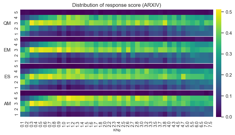
The distribution of the response score is shown for ARXIV in Figure 2. We split the dataset into subsets according to the ratio /, rounded to the first digit, and retain only the subsets which have at least 300 samples. In each subset (and for each embedding model) the sum of the values (5 vertical cells in the heatmap) equals 1.
We see that for ARXIV, the best scored responses occur at values of which are comparable to . At lower values of , there may not be enough positive texts to give a good response. At high there may be too many negative texts within , which can confuse the LLM and lead to lower scores. For ARXIV specifically, these scores may be exacerbated due to the difficulty of the dataset.
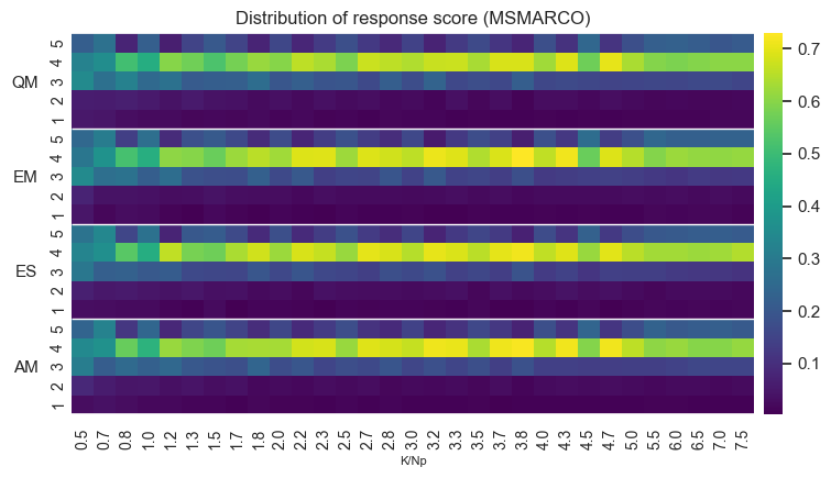
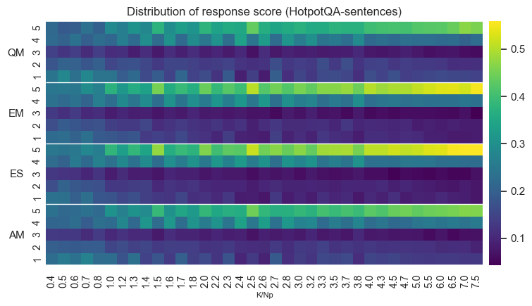
Figure 3 shows a similar pattern for MSMARCO, but with a higher “optimal” ratio of than for ARXIV. We speculate the reason for this is that MSMARCO contains texts which are simpler to understand relative to ARXIV. Therefore the detriment which comes from adding extra negatives is outweighed by the increasing likelihood of capturing more positives. This is demonstrated to a further extent with HotpotQS-sentences (Figure 4, which must be even simpler for the LLM to understand given the higher “optimal” value of .
Our observations for the Natural Questions and HotpotQA-paragraphs datasets are similar to HotpotQA-sentences, but have fewer available segments; they are shown in Appendix B.


3.2 Correlations
Spearman correlations of , and with the response score are shown in Figure 5. The datasets defined in Section 2.3 are split here into “narrow” (suffix “-n”) and “wide” (suffix “-w”), with samples having < and respectively. The Pearson and Kendall Tau correlations have similar trends and are given in Appendix C.
From Figure 1 we can see that for many of the segments considered, the measure does not lose much in terms of correlations compared to even though it is formulated without .
For a more detailed analysis, we consider more refined segments of data - splitting the datasets by the ratio , rounded to the first digit, as described in Section 3.1. Examples of the correlations from ARXIV on such segments are shown in Figure 6 for the measure. The level of correlations between and the response score is similar for other datasets (Appendix C.3). The correlations between and the response score are also not very different (Appendix C.3). For this reason, in the next Section we show the differences between the correlations.
3.3 Differences between measures
Table 2 gives an overview of the Spearman correlations for , and as the dataset, embedding model and are varied. In general, we see that performs best for ARXIV and HotPotQA-sentences in the low regime and is overtaken by and as increases. For MSMARCO and Natural Questions, appears to outperform both and for all values of tested.
Figures 7, 8 and 9 show the difference between the correlations of with the response score and with the response score. The difference depends more on the data than on the embeddings. Specifically, for ARXIV and HotpotQA-sentences, the measure correlates better with the response score than on most segments; for MSMARCO it is worse. The results for HotpotQA-paragraphs and Natural Questions are not shown because there is no noticeable difference for them.
The simpler, unnormalized version of (, Equation 4) has worse correlations with the response quality score on ARXIV (Figure 10) and on HotpotQA-sentences (Figure 11), has mixed and less difference on MSMARCO (Figure 12) and has no noticeable difference on HotpotQA-paragraphs and on Natural Questions.
For the majority of the datasets, shows worse correlations relative to , but gets better for high in ARXIV (Figure 13).
We suggest the reason lies in the complexity of the ARXIV abstracts, which yields greater benefits when the top findings are presented to the LLM in an easier order: first relevant, then non-relevant. The order becomes especially important for high ratio, when there are inevitably many negative (irrelevant) items within top . A similar trend can be seen for MSMARCO (Figure 14) and Natural Questions (Figure 15); however for these datasets, is still worse than . The trend is less pronounced for HotpotQA (see Figures 33 and 34 and Appendix D), possibly because HotpotQA-sentences samples are too simple and because the range of for HotpotQA-paragraphs is too narrow.
In Figures 16 and 17, we see similar trend appearing for ( with replaced by a crude estimate - within ) when evaluating on ARXIV and MSMARCO. The reason here, we assume, is that the estimate of , however primitive, is still more reliable at higher ratios , simply because the top documents have more positives. The comparisons on other datasets are more limited, and shown in Figures 35 and 36 in Appendix D (no noticeable difference on HotpotQA-paragraphs, not shown).
It is surprising, however, that at high ratios of can become even better than , meaning that an estimated serves better than the real . We suspect the reason is that the relevant documents falling into the top (used in our estimation of ) are more important and should “weigh more” than other relevant documents when counting . Because these documents happen to be closer to the query (by embedding similarity), it is likely they also would be easier for the LLM and more useful, especially at high .
As we already observed (Figures 13, 14, 15, 33, 34), is mostly worse that , except at high values for ARXIV - when the content is difficult and the order of numerous negatives (irrelevant documents) within top is important for the LLM. Since is better or not too different from (Figures 7, 8 and 9), is also better than at not too high values for ARXIV (Figure 18); it is also better than for other datasets (Figures 38, 37, 39 and 40 in Appendix D).
4 Conclusion
We considered a few measures representing different approaches to using , the total count of documents relevant to a query. Measure requires knowing , which can be achieved by labeling and fixing part of KB. Measures (suggested here) and do not use . Measure uses a crudely estimated value for . We compared how well these measures correlate with a quality score, assigned (by an LLM) to a response generated (by an LLM) from the top retrieved documents. Our conclusions:
-
1.
Only at high ratios, as the order of documents within top- becomes too important for the LLM, may become better than or on a dataset with complicated enough documents (ARXIV).
-
2.
Except the above, the measure is better than , and similar to (and at low or moderate can be better, depending on a dataset).
-
3.
At high ratios, substituting a simple estimate of from a selection instead of the real not just approximates , but even improves it. We suggest the reason is that the relevant documents ranked higher (and therefore falling into the top ) would be more important for the LLM response than the rest of the relevant documents.
-
4.
Within our observations, the document type and the ratio appear to be more important than the choice of an embedding model when selecting a retrieval measure (and simply for the response score).
Of course in practice, the range of depends on the distribution of in the used data, the choice of (which may be varied at runtime depending on a query and the retrieved texts) and on a consideration of computation expenses and time lag (growing with ).
Limitations
Our experiments focus on retrieval scenarios with relatively moderate ranges of , which may limit the applicability of our findings to broader retrieval regimes.
We left out a consideration of the additional latency incurred when evaluating the results of a retrieval in realtime. The measures (even not involving a knowledge of ) require identifying relevancy of the top- documents with respect to a query. Outside of using a fixed query with a corresponding set of labeled documents, one direct method of obtaining labels is by using an LLM to assess the relevancy of each document to the query after making the top- selection. This is particularly useful in a retrieval system monitoring setting, where any additional time spent measuring the quality of a retrieval will not block any downstream tasks–the system simply continues on while the results are recorded in the background.
References
- Can we use large language models to fill relevance judgments?. arXiv:2405.05600. External Links: Link Cited by: item 2.
- The distracting effect: understanding irrelevant passages in RAG. In Proceedings of the 63rd Annual Meeting of the Association for Computational Linguistics (Volume 1: Long Papers), W. Che, J. Nabende, E. Shutova, and M. T. Pilehvar (Eds.), Vienna, Austria, pp. 18228–18258. External Links: Link, Document, ISBN 979-8-89176-251-0 Cited by: §1.
- MS MARCO: A human generated MAchine Reading COmprehension dataset. arXiv:1611.09268. External Links: Link Cited by: item 4.
- Nearly optimal capture-recapture sampling and empirical likelihood weighting estimation for M-estimation with big data. arXiv:2209.04569. External Links: Link Cited by: §1.
- Towards meaningful statements in IR evaluation. mapping evaluation measures to interval scales. arXiv:2101.02668. External Links: Link Cited by: §1.
- Population size estimation with capture-recapture in presence of individual misidentification and low recapture. arXiv:2304.00885. External Links: Link Cited by: item 2.
- Query-specific variable depth pooling via query performance prediction towards reducing relevance assessment effort. arXiv:2304.11752. External Links: Link Cited by: item 2.
- What makes a good order of examples in in-context learning. In Findings of the Association for Computational Linguistics: ACL 2024, L. Ku, A. Martins, and V. Srikumar (Eds.), Bangkok, Thailand, pp. 14892–14904. External Links: Link, Document Cited by: §1.
- IR evaluation methods for retrieving highly relevant documents. In Proceedings of the 23rd Annual International ACM SIGIR Conference on Research and Development in Information Retrieval, SIGIR ’00, New York, NY, USA, pp. 41–48. External Links: ISBN 1581132263, Link, Document Cited by: §1, §2.1.
- Cumulated gain-based evaluation of IR techniques. 20 (4), pp. 422–446. External Links: ISSN 1046-8188, Link, Document Cited by: §1, §2.1.
- Fact, fetch, and reason: a unified evaluation of retrieval-augmented generation. In Proceedings of the 2025 Conference of the Nations of the Americas Chapter of the Association for Computational Linguistics: Human Language Technologies (Volume 1: Long Papers), L. Chiruzzo, A. Ritter, and L. Wang (Eds.), Albuquerque, New Mexico, pp. 4745–4759. External Links: Link, Document, ISBN 979-8-89176-189-6 Cited by: item 2.
- Intelligent topic selection for low-cost information retrieval evaluation: a new perspective on deep vs. shallow judging. 54 (1), pp. 37–59. External Links: ISSN 0306-4573, Document, Link Cited by: §1.
- Natural questions: a benchmark for question answering research. 7, pp. 452–466. External Links: Link, Document Cited by: item 5.
- How does knowledge selection help retrieval augmented generation?. arXiv:2410.13258. External Links: Link Cited by: §1.
- Input order shapes LLM semantic alignment in multi-document summarization. arXiv arXiv:2512.02665. External Links: Link Cited by: §1.
- QA-RAG: Exploring LLM reliance on external knowledge. Big Data and Cognitive ComputingProceedings of the AAAI Conference on Artificial IntelligencearXivTransactions of the Association for Computational LinguisticsarXivACM Trans. Inf. Syst.arXivarXivInformation Processing & ManagementarXivarXivarXivarXivarXivarXivarXivarXivarXivarXivJournal of DocumentationAdvances in Artificial Intelligence and Machine LearningarXivTransactions of the Association for Computational LinguisticsACM Comput. Surv.ArXivInf. Retr.arXivarXivarXivarXivarXivarXiv 8 (9). External Links: Link, ISSN 2504-2289 Cited by: §1.
- Mark-evaluate: assessing language generation using population estimation methods. arXiv:2010.04606. External Links: Link Cited by: item 2.
- Active testing: an efficient and robust framework for estimating accuracy. External Links: Link Cited by: §1.
- Comparing the sensitivity of information retrieval metrics. In Proceedings of the 33rd International ACM SIGIR Conference on Research and Development in Information Retrieval, SIGIR ’10, New York, NY, USA, pp. 667–674. External Links: ISBN 9781450301534, Link, Document Cited by: §1.
- Breaking the lens of the telescope: online relevance estimation over large retrieval sets. arXiv:2504.09353. External Links: Link Cited by: item 2.
- Sentence-BERT: sentence embeddings using Siamese BERT-networks. In Proceedings of the 2019 Conference on Empirical Methods in Natural Language Processing and the 9th International Joint Conference on Natural Language Processing (EMNLP-IJCNLP), K. Inui, J. Jiang, V. Ng, and X. Wan (Eds.), Hong Kong, China, pp. 3982–3992. External Links: Link, Document Cited by: item 1.
- A theoretical basis for the use of co-occurence data in information retrieval. 33 (2), pp. 106–119. External Links: Link Cited by: §1.
- Effective data pruning through score extrapolation. arXiv:2506.09010. External Links: Link Cited by: item 2.
- Capturing collection size for distributed non-cooperative retrieval. In Proceedings of the 29th Annual International ACM SIGIR Conference on Research and Development in Information Retrieval, SIGIR ’06, New York, NY, USA, pp. 316–323. External Links: ISBN 1595933697, Link, Document Cited by: §1.
- A comparison of pooled and sampled relevance judgments. In Proceedings of the 30th Annual International ACM SIGIR Conference on Research and Development in Information Retrieval, SIGIR ’07, New York, NY, USA, pp. 785–786. External Links: ISBN 9781595935977, Link, Document Cited by: §1.
- LLM-assisted relevance assessments: when should we ask LLMs for help?. In Proceedings of the 48th International ACM SIGIR Conference on Research and Development in Information Retrieval, SIGIR ’25, New York, NY, USA, pp. 95–105. External Links: ISBN 9798400715921, Link, Document Cited by: item 2.
- LLMs can patch up missing relevance judgments in evaluation. arXiv:2405.04727. External Links: Link Cited by: item 2.
- Assessing ranking metrics in top-N recommendation. 23 (4), pp. 411–448. External Links: ISSN 1386-4564, Link, Document Cited by: §1.
- Information retrieval. Second edition, Butterworths, London. Cited by: §1, §2.1.
- Text embeddings by weakly-supervised contrastive pre-training. arXiv:2212.03533. External Links: Link Cited by: item 3.
- Multilingual E5 text embeddings: a technical report. arXiv:2402.05672. External Links: Link Cited by: item 2.
- A theoretical analysis of NDCG type ranking measures. arXiv:1304.6480. External Links: Link Cited by: §2.1.
- Approximate recall confidence intervals. arXiv:1202.2880. External Links: Link Cited by: §1.
- Improving retrieval augmented language model with self-reasoning. 39 (24), pp. 25534–25542. External Links: Link, Document Cited by: §1.
- HotpotQA: a dataset for diverse, explainable multi-hop question answering. In Proceedings of the 2018 Conference on Empirical Methods in Natural Language Processing, E. Riloff, D. Chiang, J. Hockenmaier, and J. Tsujii (Eds.), Brussels, Belgium, pp. 2369–2380. External Links: Link, Document Cited by: §2.3.
- Estimating average precision with incomplete and imperfect judgments. In Proceedings of the 15th ACM International Conference on Information and Knowledge Management, CIKM ’06, New York, NY, USA, pp. 102–111. External Links: ISBN 1595934332, Link, Document Cited by: §1.
- How reliable are the results of large-scale information retrieval experiments?. In Proceedings of the 21st Annual International ACM SIGIR Conference on Research and Development in Information Retrieval, SIGIR ’98, New York, NY, USA, pp. 307–314. External Links: ISBN 1581130155, Link, Document Cited by: §1.
Appendix A Dataset Retrieval-Response
A.1 Data
The dataset888https://huggingface.co/datasets/primer-ai/retrieval-response consists of four parts:
-
1.
Query-texts samples
-
2.
Ranked samples
-
3.
Graded samples
-
4.
Human-graded samples
A.1.1 Query-texts samples
Query-texts samples consist of 6112 samples, each sample is a dictionary with the following items:
-
1.
“id”: A string Id of the sample. The Id consists of a name of a subset, concatenated by “-” with Id of the item in the subset. For example, Id=“N-5” means that it is sample #5 from the subset Natural Questions. Each sample is uniquely identified by its Id.
-
2.
“q”: The query.
-
3.
“p”: The list of positives.
-
4.
“n”: The list of negatives.
All the subsets in the dataset: “A”, “Hp-e”, “Hp-h”, “Hp-m”, “Hs-e”, “Hs-h”, “Hs-m”, “M”, “N”. The short names, as explained in Section 2, are “A” for ARXIV, “H” for HotpotQA, “M” for MSMARCO and “N” for Natural Questions.
HotpotQA appears with two different granularities: The positives and negatives are (1) paragraphs in “Hp” and (2) sentences in “Hs”. Beyond that, we keep the HotpotQA classification of the queries: easy (suffix “-e”), medium (“-m”) and hard (“-h”).
In the ARXIV sample, a query is a name of an arxiv category. The positives are abstracts of papers in this category and the negatives are abstracts of papers in a related, but different category. We kept the following additional, not strictly necessary, information, with additional keys:
-
1.
“c1”: The symbolic name of a category for positives. (The name of this category serves as the query and is stored with the key “q”.)
-
2.
“c2”: The symbolic name of a category for negatives.
-
3.
“q2”: The name of the category for negatives (not used).
For example, a sample with id=“A-0” has c1=“math.ca”, c2=“math.pr”, q=“classical analysis and ODEs” and q2=“probability” (it also has a list of positives “p” and a list of negatives “n”).
A.1.2 Ranked samples
Each of the query-texts samples (Appendix A.1.1) can be used as a retrieval example with different number of candidates, number of positives (<), number of top retrieved texts, and the retrieval can be done with different embeddings.
The number of ranked samples is 42992; each of the four embeddings (listed in Section 2) is used in 10748 samples. Each ranked sample is a dictionary with the following items:
-
1.
“id”: A string Id of the sample, the same as in the query-texts samples.
-
2.
“E”: The embedding’s short notation, as specified in Section 2. The embedding used for ranking of all the candidates and selecting top-K candidates.
-
3.
“Nc”: Total number of candidates (positives and negatives), taken from the corresponding query-texts sample (with the same “id”).
-
4.
“Np”: Total number of positives, taken as the first positives “p” of the corresponding query-texts sample. (Negatives are also taken as first - from the negatives “n”.)
-
5.
“K”: A sorted list of all the (number of retrieved candidates, “top-K”) used for this sample.
-
6.
“P”: A list of precisions calculated for the top-K specified in the list “K”, in the same order. Has the same length as the list “K”.
-
7.
“R”: A list of recalls calculated for the top-K specified in the list “K”, in the same order.
-
8.
“rank”: A list (length ) of indexes of all the candidates, sorted by ranks accordingly to cosine similarities with query, by the embedding “E”.
Each ranked sample is uniquely identified by the tuple (, , , ).
In order to get the ranked texts corresponding to the “rank” list of a ranked sample , its query-texts sample (the sample with the same “id”) can be used as in this snippet:
To assure an understanding of the data of a ranked sample and of the corresponding query-texts sample , see the following assertions:


A.1.3 Graded samples
The LLM grading is done for each choice of “top-K” in each of the ranked samples. This means that each ranked sample makes len([’K’]) graded samples. In total, this gives 535888 graded samples.
The grading is done as outlined in Section 2; more details and the prompts are in Appendices A.2 and A.3. Each graded sample is a dictionary with the following items, most of which are familiar from the ranked samples:
-
1.
“id”: A string Id of the sample, the same as in the query-texts samples.
-
2.
“E”: The embedding’s short notation.
-
3.
“Nc”: Total number of candidates (positives and negatives).
-
4.
“Np”: Total number of positives.
-
5.
“K”: A value of K (“top-K”) taken from the list of “K” in the corresponding ranked sample.
-
6.
“rank”: A list equal to the first K elements of the list “rank” of the corresponding ranked sample , i.e. Sr[“rank”][:K].
-
7.
“inK”: A list created from the “rank” (the item above), by replacement of each index by 1 (if positive) or 0 (if negative).
-
8.
“answer_ideal”: LLM-generated answer to the query, obtained by using all the positives from the corresponding query-texts sample.
-
9.
“answer_topK”: LLN-generated answer to the query, obtained by using the retrieved candidates, given to LLM in their ranking order.
-
10.
“grade”: The LLM-generated score (on Linkert scale from 1 to 5), obtained by comparing the top-K answer to the ideal answer, with the knowledge of the query.
-
11.
“P”: A value of precision corresponding to the selected ; given here for convenience.
-
12.
“R”: A value of recall corresponding to the selected ; given here for convenience.
Each graded sample is uniquely identified by the tuple (, , , , ) and it is related to its ranked sample by the tuple (, , , ). To assure an understanding of the data of a graded sample and of the corresponding ranked sample , see the following assertions:
A.1.4 Human-graded samples
This part consists of 96 samples taken from the Graded Samples (Appendix A.1.3) and graded by humans. This part was used for estimating Krippendorff coefficients (Section 2.5. Each sample has already introduced data fields (, , , , , , , , ) and the human scores: , where =1,2,3 corresponds to Id of the human.
A.1.5 Dataset content
Each subset of the retrieval-response dataset has comparable amounts of samples with a different number of candidates , total number of positives and choice of , subject to the availability in the sources we used. Table 3 gives a summary of the dataset content: the number of ranked samples for each embedding, subset, , and a range of the selection (“top-K”) choices . The embedding model is not specified, because the numbers of samples are the same for each embedding.
| subset | ||||
|---|---|---|---|---|
| A | 50 | 2 | [2,15] | 300 |
| 50 | 3 | [2,15] | 300 | |
| 50 | 4 | [2,15] | 300 | |
| 50 | 5 | [2,15] | 300 | |
| 50 | 10 | [2,15] | 300 | |
| 50 | 15 | [2,20] | 300 | |
| 100 | 5 | [2,15] | 300 | |
| 100 | 10 | [2,15] | 300 | |
| 100 | 15 | [2,20] | 300 | |
| Hp | 10 | 2 | [2,5] | 900 |
| Hs | 10 | 2 | [2,5] | 900 |
| 30 | 5 | [2,15] | 719 | |
| 50 | 2 | [2,15] | 900 | |
| 50 | 3 | [2,15] | 900 | |
| 50 | 4 | [2,15] | 803 | |
| 50 | 5 | [2,15] | 298 | |
| 30 | 6 | [2,15] | 231 | |
| M | 30 | 2 | [2,15] | 300 |
| 30 | 3 | [2,15] | 300 | |
| 30 | 4 | [2,15] | 300 | |
| 30 | 5 | [2,15] | 62 | |
| 50 | 2 | [2,15] | 300 | |
| 50 | 3 | [2,15] | 300 | |
| 50 | 4 | [2,15] | 199 | |
| 50 | 5 | [2,15] | 36 | |
| N | 20 | 2 | [2,10] | 300 |
| 30 | 2 | [2,15] | 300 |
Table 4 shows how the samples are split between the narrow () and wide () parts of the subsets.
| subset | ||||
|---|---|---|---|---|
| A | 2700 | 40800 | 15300 | 25500 |
| Hp | 900 | 3600 | 0 | 3600 |
| Hs | 4751 | 57514 | 6481 | 51033 |
| M | 1797 | 25158 | 1892 | 23266 |
| N | 600 | 6900 | 0 | 6900 |
A.2 Response generation
The following prompt is used during the Response Generation phase. Given a query and a set of reference documents, the model must generate a response based only on the provided references, without introducing external knowledge.
System Message
User Message
A.3 Quality score generation
In the Quality Score Generation phase, an LLM evaluator compares a generated response to its ideal reference response. The model returns a discrete score from 1–5, following the rubric below, to measure content completeness and alignment.
System Message
User Message
A.4 LLM vs Human quality scores
In Section 2.5 the LLM grade was compared with human grading by Krippendorff alpha (ordinal) coefficient. Here in Table 5 we show Spearman correlations, on the same 96 human scored samples.
| LLM | H1 | H2 | H3 | |
|---|---|---|---|---|
| LLM | 0.83 | 0.83 | 0.83 | |
| H1 | 0.83 | 0.90 | 0.81 | |
| H2 | 0.83 | 0.90 | 0.79 | |
| H3 | 0.83 | 0.81 | 0.79 |
Appendix B Response Score
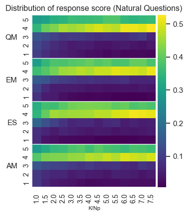
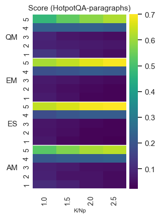
In Section 3.1 we have shown the distribution of the response score for ARXIV, MSMARCO and HotpotQA-sentences. Here we show the distributions for Natural Questions (Figure 19) and HotpotQA-paragraphs (Figure 20). They show the same simple pattern as HotpotQA-sentences: the larger the ratio , the better the response score, meaning that the texts are simple enough for LLM and negative samples are not as important as catching more positives within the range we consider.
Appendix C Correlations with response score
For convenience a script is available999https://github.com/PrimerAI/primer-research
C.1 Correlations max by
The measures and (Equations 1 and 3) depend on choice of the parameter . As we noted in Section 2.4, for a fair comparison of measures, for each measure and each data segment we consider a maximal value of a correlation (between a measure and the response score), as achieved over a range of the parameter .
Through the paper we presented results for data segments defined by the embedding, the dataset and the condition between and (Section 3.2). A crude condition is a split on samples with vs . A more refined condition is by the ratio , rounded to the first digit.
The search for maximal correlation is done over the grid of 702 values of :
-
1.
The edge values and .
-
2.
350 values obtained by raising 0.95 to the power from [1, 2, …, 350].
-
3.
350 values obtained by subtracting the above from 1.
C.2 Narrow and wide subsets
In Section 3.2 the Spearman correlations of the measures , and are shown in Figure 5. Here we show the corresponding Pearson and Kendall Tau correlations in Figures 21, 22, 23.


C.3 Subsets by
Appendix D Differences between measures
In this Section we show more heatmaps illustrating the differences between the measures - for the comparisons that were not decisive enough to be put in the main body of the paper.
Comparison of and on HotpotQA-sentences is shown in Figure 35, and on Natural Questions in Figure 36. There is no noticeable difference on HotpotQA-paragraphs (not shown).


Comparisons between and was shown for ARXIV in Figure 18. Here it is shown for other datasets in Figures 37, 38, 39, 40.


