[orcid=0000-0002-0612-9003] \cormark[1] \creditConceptualization, Methodology, Formal analysis, Writing – original draft
Software, Validation
Supervision, Writing – review & editing, Funding acquisition
1]organization=Department of Nuclear Engineering and Engineering Physics, University of Wisconsin–Madison, addressline=, city=Madison, postcode=53706, state=WI, country=USA
2]organization=Lucid Motors, addressline=7373 Gateway Blvd, city=Newark, postcode=94560, state=CA, country=USA
[1]Corresponding author.
Machine Learning Methods for Sub-Pixel Trajectory Reconstruction in Discretized Position Detectors
Abstract
We evaluate machine-learning methods for sub-pixel position and angular reconstruction in segmented particle detectors. Using cosmic-ray muon events simulated in Geant4 for an 88 scintillator array, we compare four reconstruction approaches: a transformer neural network, a convolutional neural network (CNN), a multilayer perceptron (MLP), and an energy-weighted centroid. The transformer and CNN produce median position errors of 0.18 and 0.23 cm, respectively, corresponding to approximately 3% of the 6.25 cm cell width, and median angular errors of 0.21∘ and 0.29∘. Relative to the centroid method, these correspond to six- to eightfold reductions in median position error and five- to sevenfold reductions in median angular error. Their bootstrap confidence intervals overlap for both position and angular RMSE, while both neural networks outperform the centroid reconstruction. These results show that learned reconstruction methods can recover sub-pixel position information and improve trajectory reconstruction in segmented detectors for muon tomography and cosmic-ray measurements.
keywords:
Particle tracking detectors \sepMuon tomography \sepNeural networks \sepTransformer architecturesMachine learning recovers sub-pixel muon position in a segmented scintillator array.
A hybrid transformer splits reconstruction into cell classification and offset regression.
Transformer and CNN cut median position and angular error 5–8 versus the energy-weighted centroid.
The transformer median position error is 3% of the 6.25 cm cell width.
1 Introduction
Muon tomography uses penetrating cosmic-ray muons to image dense materials and large structures [1, 2]. Applications include the detection of shielded nuclear materials, geological surveys of volcanic structures, archaeological investigations, and structural monitoring [1, 3]. The field has progressed from early feasibility studies [4] to measurements that resolved meter-scale voids within large structures [5]. Further improvements in spatial and angular resolution would extend the range of structures that can be imaged and reduce the exposure required to form a useful tomographic reconstruction.
Muon tomography reconstructs particle trajectories from hit positions measured in multiple detector planes. In a pixelated scintillator detector, however, the signal from a single muon can be distributed across several cells. The resulting light pattern does not directly specify the muon’s crossing point and therefore limits the spatial resolution obtained from the discrete detector geometry. As a charged particle traverses a scintillator, it excites the material along its path, and the subsequent de-excitation produces visible light [6, 7]. Because the array is coarsely segmented, an inclined muon and its secondary particles can deposit energy in more than one cell, so the measured multi-cell signal pattern must be used to estimate the underlying particle position.
A conventional position estimator is the energy-weighted centroid [8, 9]:
| (1) |
where is the energy recorded in cell , and are the cell coordinates. The centroid is inexpensive to compute, but its fixed functional form does not capture all spatial correlations in the detector response. It can also produce systematic position errors near cell boundaries, where multi-cell energy deposition from inclined tracks and secondary particles shifts the energy-weighted average away from the true crossing point.
Machine-learning methods provide an alternative means of estimating particle position from segmented detector signals [10]. Convolutional neural networks (CNNs) learn spatial features from image-like inputs [11] and have been applied to sub-pixel reconstruction in pixelated detectors [12]. Neural networks have also been used for charged-particle tracking in high-energy physics, including graph neural networks that associate detector hits with candidate tracks [13]. Transformer architectures were originally developed for sequence modeling [14]. Recent studies have applied transformers to charged-particle tracking in collider detectors, including hit-to-track association and joint hit filtering and track reconstruction [15, 16]. These methods operate on sparse detector-hit sets and address the combinatorial assignment of hits to tracks rather than sub-pixel position regression from two-dimensional scintillator signal patterns. In scintillator-based muon tomography, sub-pitch resolution has also been demonstrated using triangular strips and charge-centroid reconstruction [17]. The present work instead evaluates whether learned models can recover sub-pixel crossing positions directly from the signal map of a coarse, segmented scintillator array.
In this work, we investigate whether a transformer can improve position and trajectory reconstruction in a pixelated scintillator array used for muon tomography. The proposed architecture separates the task into coarse cell classification and sub-pixel offset regression. Using cosmic-ray muon events simulated in Geant4 for an 88 segmented detector array, we compare the transformer with a CNN, an MLP, and an energy-weighted centroid.
2 Detector simulation

The simulated tomography system contains four detector planes arranged as two tracking pairs, as shown in figure 1. The reconstruction study uses one representative pair of planes separated by 30 cm. The detector geometry is identical for both pairs; readout electronics are not modeled. In this work, crossing-position labels were generated only for the selected upper pair, so the reconstruction was evaluated on that pair.
We simulated the detector with Geant4 version 11.4.1 [18, 19] using the FTFP_BERT hadronic physics list together with Geant4 optical physics. Each detector plane is a cm2 polyvinyltoluene (PVT) scintillator segmented into an array of 64 cells. Each cell measures cm3.
The source generates negative muons with kinetic energies sampled from a Gaussian distribution centered at 4 GeV with GeV. Energies below 1 GeV are set to 1 GeV. The polar angle is sampled from a Gaussian distribution with rad and limited to 0.5 rad, while the azimuthal angle is sampled uniformly. This simplified source retains the characteristic energy scale of cosmic-ray muons [20] while providing a controlled dataset for comparing the reconstruction methods.
The simulation tracks scintillation-light generation and optical-photon transport. For each event, the optical-photon energy reaching a cell boundary is accumulated to form the 64-cell signal pattern. Each cell is treated as an isolated, fully absorbing counter: its surfaces have zero reflectivity, so a photon is recorded in the cell in which it was produced and transported. Inter-cell optical crosstalk and photodetector light-sharing are therefore not modeled, and multi-cell signal patterns arise only from the muon and its secondary particles depositing energy in more than one cell. Photodetectors and their electronics are not modeled explicitly. Instead, the simulation uses an effective scintillation yield of 1000 photons/MeV, approximately 10% of the intrinsic PVT light yield of 10,000 photons/MeV, to represent the combined reduction associated with light collection and photon detection. Events are retained when the primary muon intersects both planes in the selected tracking pair. The simulated crossing positions define the true trajectory and angle used to evaluate the reconstruction methods.
We generated 100,000 muon events, of which 95,262 intersected both selected detector planes. These events were divided into training, validation, and test sets using a 64%/16%/20% split, yielding 60,967, 15,242, and 19,053 events, respectively. The validation set was used for neural-network model selection and for early stopping during transformer training. All four reconstruction methods were evaluated on the same held-out test set. Each event contains the simulated muon position on both planes and the corresponding 64-cell scintillation-light signal pattern.
3 Reconstruction methods
The MLP, CNN, and transformer use 88 signal maps normalized by the total recorded energy in each event. The MLP and CNN were trained with the Adam optimizer [21], a batch size of 64, and an L2 distance loss given by the Euclidean distance between the reconstructed and true positions. The transformer was trained with AdamW and a composite loss containing cell-classification, offset-regression, and absolute-position terms, as described below. It used the same batch size of 64.
3.1 Centroid method
The centroid baseline applies equation 1 independently to each detector plane. This estimator assumes that the recorded signal is distributed symmetrically around the muon crossing point. Multi-cell energy deposition near cell boundaries and the elongated signal patterns produced by inclined tracks and secondary particles can violate this assumption and shift the reconstructed position. The trajectory angle is calculated from the two reconstructed plane positions and the known plane separation.
3.2 Multilayer perceptron
The MLP maps the flattened 64-element signal vector to continuous coordinates. Its architecture is
This model provides a learned baseline without imposing an explicit two-dimensional spatial structure on the input.
The MLP was trained for 500 epochs with a learning rate of and L2 weight decay of . The trajectory angle is calculated geometrically from the positions reconstructed on the two planes.
3.3 Convolutional neural network
The CNN retains the two-dimensional arrangement of the scintillator signal map. It contains two convolutional layers followed by fully connected regression layers, as shown in figure 2.

The first convolutional layer has 16 filters with 33 kernels and ReLU activation. The second has 32 filters with the same kernel size and activation. Padding preserves the 88 feature-map dimensions so that information from cells at the detector boundary is retained. Both convolutional layers use 10% dropout. The resulting features are flattened and passed through a 64-unit fully connected layer with ReLU activation, followed by a two-unit output layer for the reconstructed position.
The CNN was trained for 120 epochs with a learning rate of and L2 weight decay of . The checkpoint with the lowest validation distance error was retained for evaluation.
3.4 Transformer neural network
The hybrid transformer separates position reconstruction into coarse cell classification and in-cell offset regression. The classification head identifies the cell containing the simulated crossing point, and the offset head estimates the position within that cell.
A convolutional stem converts the 88 signal map into 64 tokens, one for each detector cell, and learned positional embeddings encode their locations. The tokens are processed by a four-layer transformer encoder with eight attention heads and an embedding dimension of 128. Self-attention allows each token to incorporate information from every cell in the signal map, including nonlocal correlations that are not covered by the receptive field of the two-layer CNN.
The network has two prediction heads: a cell-classification head and an in-cell offset-regression head. The in-cell coordinates are normalized to cell widths. During training, a third auxiliary term stabilizes the absolute coordinate scale; it is evaluated from the true cell center plus the predicted offset rather than from an independently regressed absolute position. The total loss is
which gives the offset-regression term the largest weight. The classification term uses cross-entropy with label smoothing of 0.05.
The transformer was trained with AdamW [22], a learning rate of , weight decay of , and cosine annealing after a five-epoch linear warmup. Gradients were clipped to a maximum norm of 1.0. Training continued for at most 120 epochs, with early stopping after 10 epochs without improvement in the validation distance error.
4 Results and discussion
We evaluated the four reconstruction methods on the held-out test set of 19,053 events, corresponding to 20% of the 95,262 events that intersected both selected detector planes. Tables 1–5 report the angular, position, track-length, confidence-interval, and per-plane results.
| Metric | Transformer | CNN | MLP | Centroid |
| Mean bias () | ||||
| Std deviation () | ||||
| RMSE () | ||||
| Median error () | ||||
| 68th percentile () | ||||
| 95th percentile () | ||||
| 99th percentile () |
| Metric | Transformer | CNN | MLP | Centroid |
| Mean () | ||||
| Std deviation () | ||||
| RMSE () | ||||
| Median error () | ||||
| 68th percentile () | ||||
| 95th percentile () | ||||
| 99th percentile () |
| Metric | Transformer | CNN | MLP | Centroid |
| Mean () | ||||
| Std deviation () | ||||
| RMSE () |
| Metric | Transformer | CNN | MLP | Centroid |
| Angular RMSE () | 1.99 [1.79, 2.19] | 1.67 [1.54, 1.80] | 1.80 [1.69, 1.92] | 2.70 [2.64, 2.77] |
| Angular median err () | 0.212 [0.208, 0.215] | 0.294 [0.289, 0.299] | 0.407 [0.400, 0.415] | 1.495 [1.461, 1.527] |
| Position RMSE () | 0.720 [0.648, 0.797] | 0.640 [0.602, 0.684] | 0.712 [0.676, 0.747] | 1.793 [1.775, 1.812] |
| Position median () | 0.181 [0.179, 0.183] | 0.231 [0.229, 0.233] | 0.301 [0.298, 0.303] | 1.432 [1.422, 1.442] |
| Metric | Transformer | CNN | MLP | Centroid |
| Plane 1 RMSE () | ||||
| Plane 1 median error () | ||||
| Plane 2 RMSE () | ||||
| Plane 2 median error () |
4.1 Angular reconstruction performance
The angular RMSE values are 1.99∘ for the transformer, 1.67∘ for the CNN, 1.80∘ for the MLP, and 2.70∘ for the centroid method. The bootstrap intervals of the three learned methods overlap, whereas all three are separated from the centroid interval (table 4). Because interval overlap is not an equivalence test, these results support comparable RMSE performance among the learned methods but do not establish statistical equivalence.
The methods separate more clearly in median absolute error. The transformer reaches 0.21∘, followed by the CNN at 0.29∘, the MLP at 0.41∘, and the centroid at 1.50∘. Relative to the centroid, these values correspond to median-error reductions of 7.1, 5.1, and 3.7, respectively. The difference between the RMSE and median rankings reflects heavy-tailed error distributions: most events are reconstructed accurately, but a small number of large errors increase the RMSE.
Mean angular biases range from 0.10∘ to 0.28∘. The larger differences among the standard deviations and upper percentiles therefore arise primarily from the spread of the error distributions rather than from a uniform angular offset.
4.2 Position reconstruction performance
The CNN has the lowest position-RMSE point estimate at 0.64 cm, followed by the MLP at 0.71 cm and the transformer at 0.72 cm. Their 95% bootstrap intervals overlap, while all three are separated from the centroid result of 1.79 cm (table 4). The RMSE results therefore do not establish a clear ordering among the learned methods.
Median position error provides greater separation. The transformer reaches 0.18 cm, followed by the CNN at 0.23 cm, the MLP at 0.30 cm, and the centroid at 1.43 cm. These correspond to reductions of 7.9, 6.2, and 4.8 relative to the centroid. The transformer median is approximately 2.9% of the 6.25 cm cell width. These results show that all three learned models recover sub-cell position information, with the transformer producing the lowest typical-event error.
4.3 Track length errors
Track-length reconstruction is a weak discriminator among the methods because the fixed 30 cm plane separation is much larger than the transverse displacement between the reconstructed positions. The CNN, MLP, and centroid each have an RMSE of approximately 0.21 cm, while the transformer has an RMSE of 0.39 cm (table 3).
All four mean track-length errors are below 0.03 cm in magnitude. The transformer’s larger RMSE is associated with its tail of large plane-2 position errors. The centroid’s cell-scale position errors have less effect on track length because the longitudinal plane separation dominates the calculation.
4.4 Error analysis
4.4.1 Error distribution characteristics

Figure 3 summarizes the differences between the RMSE and typical-event metrics. The CNN has the lowest position RMSE, while the transformer has the lowest mean and median position errors. The MLP has an RMSE similar to those of the CNN and transformer but a larger median error. All three learned methods outperform the centroid in both RMSE and median position error.
The percentile results show how the error distributions broaden in their tails. For the transformer, 68% of angular errors are below 0.33∘ and 95% are below 0.93∘, compared with 2.38∘ and 4.58∘ for the centroid. At the 99th percentile, the transformer error increases to 5.18∘, indicating that a small subset of events remains difficult for every reconstruction method.
4.4.2 Spatial error patterns


Figures 4 and 5 show the spatial distribution of the reconstruction errors. On plane 1, the transformer and CNN generally produce shorter error vectors than the centroid method. The centroid errors retain a visible correlation with the segmented detector geometry, particularly near cell boundaries, where multi-cell energy deposition shifts the energy-weighted position.
Plane 2 has similar median errors but substantially larger RMSE for the learned methods. This difference indicates that the degradation is concentrated in a small number of events rather than distributed uniformly across the sample.

The plane-2 RMSE values for the neural methods are 1.15–1.36 cm, approximately four to five times their plane-1 values of 0.26–0.38 cm. Their plane-2 median errors remain between 0.17 and 0.29 cm, close to the plane-1 medians. The increased RMSE therefore arises from a tail of large errors rather than a uniform loss of precision.
In 0.92% of plane-2 events, the brightest cell is displaced by more than one cell width from the true muon position. For these events, the cell traversed by the muon contains a median of approximately 29% of the collected signal, while a spatially separated competing peak, consistent with secondary-particle activity, appears in a more distant cell. Figure 6 shows one such event. The corresponding condition occurs in 0.002% of plane-1 events. These fractions are computed over all labeled events common to both planes rather than over the held-out test set.
When the strongest signal is spatially separated from the true crossing point, any estimator based only on the 64-cell signal map faces an ambiguous input. This effect contributes to the large-error tail shared by all four methods. Plane-specific training or additional detector information may reduce these errors, but that possibility was not evaluated here.
4.4.3 Angular and position error distributions
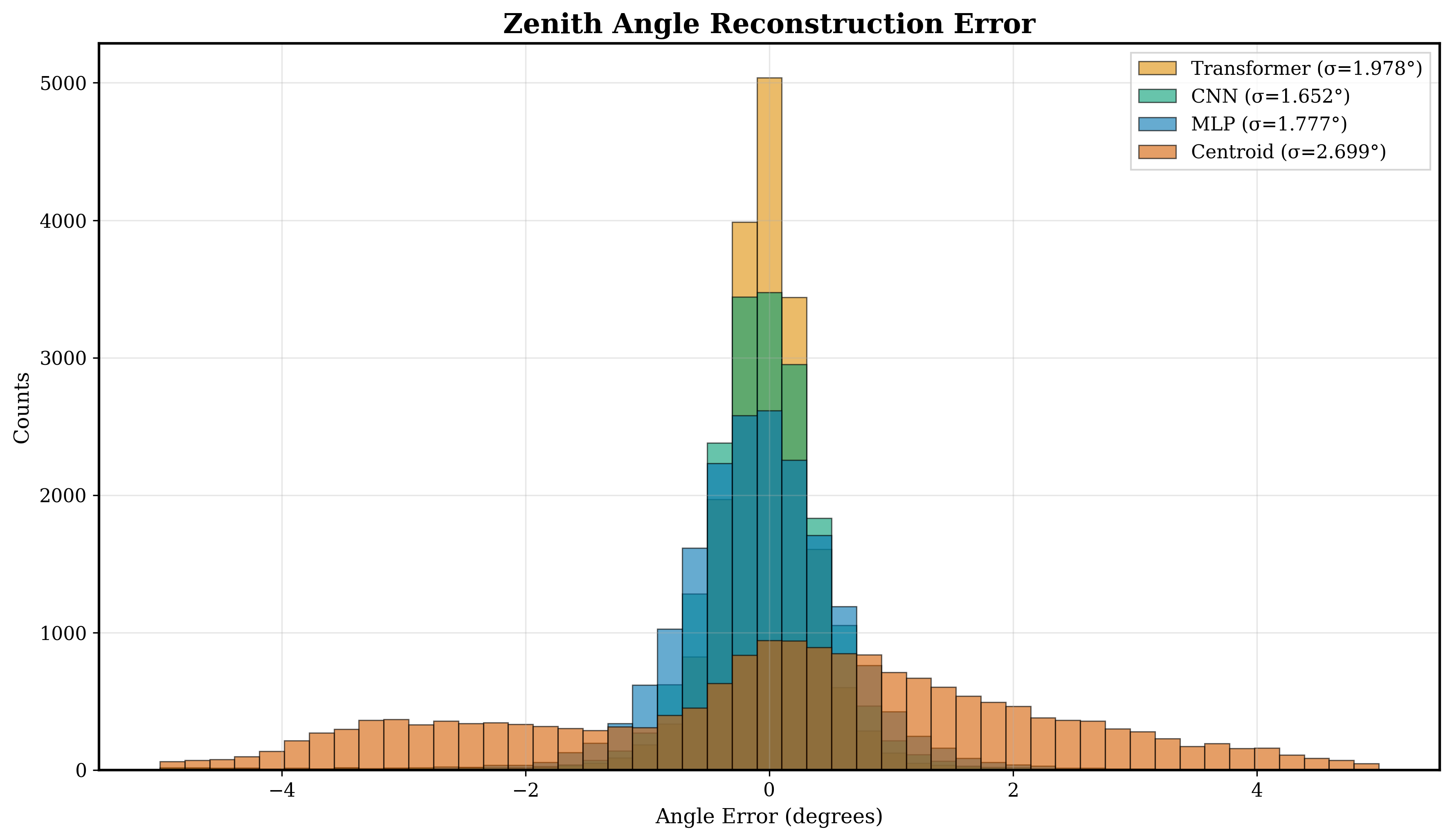
The angular error histogram (figure 7) shows a narrow central distribution for the transformer, with 95% of events below approximately 0.93∘. The broader centroid distribution reflects the propagation of position errors from both detector planes into the reconstructed angle.
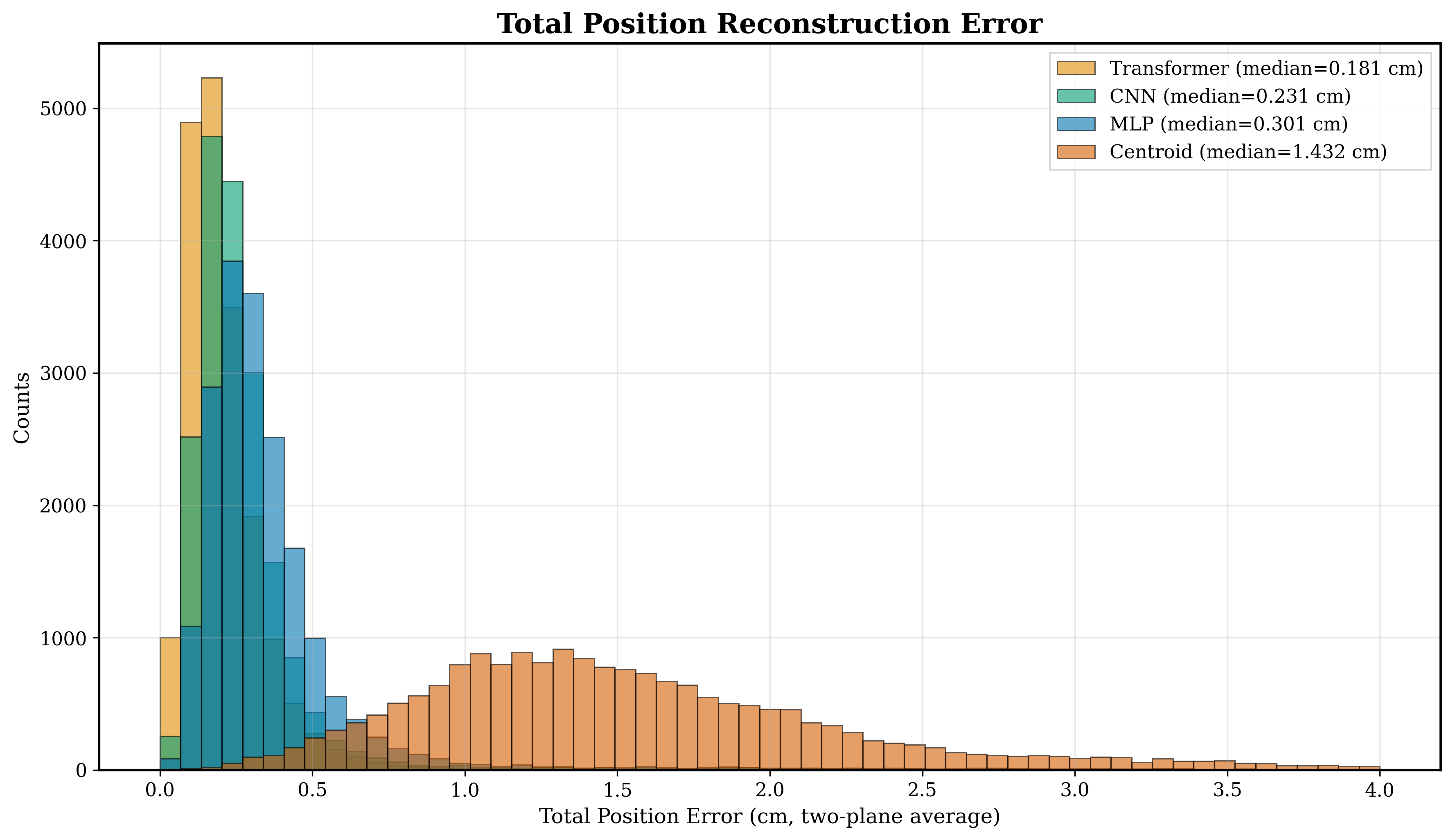
The total position-error histogram (figure 8) shows median errors of 0.18 cm for the transformer, 0.23 cm for the CNN, 0.30 cm for the MLP, and 1.43 cm for the centroid. The learned methods therefore recover sub-cell position information for typical events. Image-level improvements were not evaluated in this study, and the heavy error tails remain concentrated on the second selected detector plane.
5 Conclusions
Position uncertainty in pixelated scintillator detectors propagates directly into the reconstructed muon trajectory and scattering angle. The energy-weighted centroid is sensitive to the segmented detector geometry, particularly near cell boundaries where multi-cell energy deposition can shift the reconstructed position away from the true crossing point.
All three learned methods recover sub-cell position information from the 64-cell signal maps. The transformer and CNN produce median position errors of 0.18 and 0.23 cm, respectively, compared with 0.30 cm for the MLP and 1.43 cm for the centroid. The transformer median corresponds to approximately 2.9% of the 6.25 cm cell width. Its cell-classification and in-cell offset heads provide the lowest median position and angular errors, while the CNN has the lowest position- and angular-RMSE point estimates. The overlapping RMSE confidence intervals do not establish a statistical ordering among the learned methods.
These results show that learned reconstruction can recover position information below the cell width without changing the simulated detector geometry. The improvement is clearest in the median and lower percentiles. A small population of events with competing secondary-electron signals produces a heavy error tail, particularly on the second selected detector plane, and reduces the apparent improvement in RMSE.
This proof-of-concept study uses simulated data, a simplified cosmic-muon source, an effective scintillation yield, and no explicit model of photodetectors or readout electronics. All models were trained and tested on the same narrow, near-vertical source distribution; performance under out-of-distribution source conditions, such as wider angular or energy spectra, was not evaluated. It also evaluates trajectory errors rather than complete tomographic-image quality. Experimental validation should therefore include measured optical response, calibration variation, electronic noise, thresholds, and plane-dependent effects. Future work should also test whether plane-specific training, additional detector layers, or explicit treatment of secondary-electron events can reduce the large-error tail.
Declaration of competing interest
The authors declare that they have no known competing financial interests or personal relationships that could have appeared to influence the work reported in this paper.
Data availability
The Geant4 simulation source code, the Python analysis and reconstruction pipeline, and the derived datasets supporting this article are openly available on Zenodo at https://doi.org/10.5281/zenodo.21340841.
Acknowledgements
This work is supported by the College of Engineering and the Grainger Institute for Engineering at the University of Wisconsin–Madison. This research was supported in part by an appointment to the Oak Ridge National Laboratory GRO Program, sponsored by the U.S. Department of Energy and administered by the Oak Ridge Institute for Science and Education.
References
- [1] G. Bonomi et al., Applications of cosmic-ray muons, Prog. Part. Nucl. Phys. 112 (2020) 103768.
- [2] K.N. Borozdin et al., Radiographic imaging with cosmic-ray muons, Nature 422 (2003) 277.
- [3] J. Bae and S. Chatzidakis, The effect of cosmic ray muon momentum measurement for monitoring shielded special nuclear materials, arXiv:2109.02470 (2022).
- [4] L.W. Alvarez et al., Search for hidden chambers in the pyramids, Science 167 (1970) 832.
- [5] K. Morishima et al., Discovery of a big void in Khufu’s Pyramid by observation of cosmic-ray muons, Nature 552 (2017) 386.
- [6] G.F. Knoll, Radiation Detection and Measurement, John Wiley & Sons (2000).
- [7] C. Grupen and B. Shwartz, Particle Detectors, 2nd ed., Cambridge University Press (2008), doi:10.1017/CBO9780511534966.
- [8] V. Radeka and R.A. Boie, Centroid finding method for position-sensitive detectors, Nucl. Instrum. Methods 178 (1980) 543–554, doi:10.1016/0029-554X(80)90836-8.
- [9] G. Landi, Properties of the center of gravity as an algorithm for position measurements, Nucl. Instrum. Methods Phys. Res. A 485 (2002) 698.
- [10] Y. LeCun, Y. Bengio and G. Hinton, Deep learning, Nature 521 (2015) 436.
- [11] A. Krizhevsky, I. Sutskever and G.E. Hinton, ImageNet classification with deep convolutional neural networks, Adv. Neural Inf. Process. Syst. 25 (2012) 1097.
- [12] J.P. van Schayck et al., Sub-pixel electron detection using a convolutional neural network, Ultramicroscopy 218 (2020) 113091.
- [13] G. DeZoort et al., Charged particle tracking via edge-classifying interaction networks, Comput. Softw. Big Sci. 5 (2021) 26.
- [14] A. Vaswani et al., Attention is all you need, Adv. Neural Inf. Process. Syst. 30 (2017) 5998.
- [15] S. Caron et al., Trackformers: In search of transformer-based particle tracking for the high-luminosity LHC era, Eur. Phys. J. C 85 (2025) 460, doi:10.1140/epjc/s10052-025-14156-3.
- [16] S. Van Stroud et al., Transformers for charged particle track reconstruction in high-energy physics, Phys. Rev. X 15 (2025) 041046, doi:10.1103/md46-yqgd.
- [17] Z. Liang et al., A muon scattering tomography system based on high spatial resolution scintillating detector, Nucl. Instrum. Methods Phys. Res. A 1091 (2026) 171790, doi:10.1016/j.nima.2026.171790.
- [18] S. Agostinelli et al., Geant4—a simulation toolkit, Nucl. Instrum. Methods Phys. Res. A 506 (2003) 250.
- [19] J. Allison et al., Recent developments in Geant4, Nucl. Instrum. Methods Phys. Res. A 835 (2016) 186.
- [20] Particle Data Group, Review of Particle Physics, Phys. Rev. D 110 (2024) 030001.
- [21] D.P. Kingma and J. Ba, Adam: A method for stochastic optimization, arXiv:1412.6980.
- [22] I. Loshchilov and F. Hutter, Decoupled weight decay regularization, International Conference on Learning Representations (ICLR), 2019; arXiv:1711.05101.