Multi-Method Timing of Transient Radio Pulsars with the GBT350 and GBNCC Surveys
Abstract
We present the timing solutions for three radio pulsars discovered with the Green Bank North Celestial Cap (GBNCC) and 350-MHz Green Bank Telescope drift-scan surveys. These pulsars were initially discovered through their single-pulse emission and therefore designated as rotating radio transients (RRATs). Follow-up timing campaigns yielded a number of higher signal-to-noise summed pulse profiles for each pulsar, allowing us to obtain timing solutions both through single pulses as well as the standard method of time-integrating the pulsar’s emission. We find that the two methods return timing parameters which are usually in agreement within two standard deviations, and have similar sized error bars. The single-pulse timing solutions have significantly higher RMS errors and reduced chi-squared values, likely due to pulse jitter. The distribution of wait times between detected single pulses indicates a significant amount of pulse clustering in time on short timescales from all three sources. For all sources, the presence of low-level emission outside of the sparse bright pulses and lack of giant pulses is more reminiscent of highly nulling canonical radio pulsars than extremely transient RRATs, highlighting the diversity of emission behavior observed from sources published as RRATs.
I Introduction
Radio pulsars are rapidly rotating, highly magnetized neutron stars with beams of radio emission extending from their magnetic poles. To date, over 4000 pulsars have been discovered (see, e.g., the ATNF pulsar catalog111v 2.6.5; https://www.atnf.csiro.au/research/pulsar/psrcat/; Manchester et al. 2005). Radio pulsars are most often discovered using Fourier-domain periodicity searches, and occasionally in the time domain using fast folding algorithms (e.g. Cameron et al. 2017; Parent et al. 2018).
Rotating RAdio Transients (RRATs), sources emitting isolated radio pulses separated by intervals of minutes to hours, were discovered in single-pulse searches of survey data by McLaughlin et al. (2006). The pulses from these RRATs obey an underlying periodicity and, like standard radio pulsars, are indicative of radio emission powered by the rotational energy loss of a magnetized neutron star. RRATs are most commonly defined in the literature as pulsars discovered solely through their isolated pulses, as opposed to periodic emission (McLaughlin et al. 2006; Keane and McLaughlin 2011). If RRATs represent a distinct and separate population of neutron stars, their sporadic nature implies the potential for an enormous population of undetected RRATs, to the point that the observed Galactic supernova rate would not be sufficient to produce the expected number of neutron stars (McLaughlin et al. 2006; Keane and Kramer 2008).
The individual pulses from both pulsars and RRATs display a great deal of temporal variability in their pulse shapes and amplitudes. In addition to stochastic (random) variations of pulsed flux with time, some pulsars display sudden, discontinuous changes in their pulse shapes and fluxes. One manifestation of this phenomenon is nulling, in which the pulsar flux suddenly drops well below the detection threshold, before just as suddenly returning to its usual emission state (Wang et al., 2007; Burke-Spolaor and Bailes, 2010). Nulling pulsars display a wide range of intermittency, usually quantified by the nulling fraction, or the fraction of pulses with no detectable emission. It has been suggested that RRATs represent the extreme end of the pulsar intermittency spectrum, or manifest nulling fractions close to one (Burke-Spolaor and Bailes, 2010; Zhou et al., 2023; Gao et al., 2025). However, comparisons of the RRAT and nulling pulsar populations have shown that RRATs have longer average spin periods and lower average surface magnetic field strengths; the distributions of these quantities do not appear to be drawn from the same population as those of nulling pulsars, implying that perhaps not all RRATs are just extreme nulling pulsars (Abhishek et al., 2022).
As more sensitive telescopes are built, it will be possible to detect low-luminosity emission outside of the bright pulses from some pulsars originally identified as RRATs, allowing for their detection in periodicity searches. Using the FAST telescope, Zhou et al. (2023) characterized the emission from newly- and previously-discovered RRATs, and found that they generally fall into three categories: prototypical RRATs (sporadic, isolated bright pulses separated by long spans with no detected emission), extreme nullers (several successive pulse periods with detected pulses, separated by long time spans of no detectable emission), and standard pulsars emitting low-level emission with sporadic bright pulses. Some RRATs have been observed switching between a RRAT-like and pulsar-like emission state, further indicating how observational sensitivity and the variable emission states of RRATs and pulsars can muddy the attempts to classify these objects based on long-term properties (Burke-Spolaor and Bailes 2010; Sun et al. 2021).
The single-pulse properties of RRATs can clarify their emission states and their relationship to canonical pulsars. For instance, the distribution of pulse energies of most normal pulsars and some RRATs is best described by a log-normal distribution (e.g. Burke-Spolaor et al. 2012; Cui et al. 2017; Mickaliger et al. 2018); conversely, giant pulses with flux densities hundreds to thousands of times higher than the mean flux density have been observed from the Crab Pulsar and a handful of other pulsars, with their energy distribution following a power-law distribution (Mickaliger et al. 2012; van Leeuwen et al. 2020; Doskoch et al. 2024). Some pulsars and RRATs also show evidence of a power law tail in their energy distributions, as well as more complex pulse energy distributions (Mickaliger et al. 2018; Zhou et al. 2023).
The distribution of wait times between consecutive detected pulses can also be used as a diagnostic to probe the emission processes in pulsars and RRATs. If the wait times between detected pulses were governed by a random process, the probability distribution of the wait times would follow an exponential distribution with a constant burst rate, which has been observed in RRAT wait time distributions as well as giant pulses from the Crab pulsar (Karuppusamy et al. 2010; Shapiro-Albert et al. 2018). Some RRATs show evidence of pulse clustering on short timescales, with their wait time distributions exhibiting non-Poissonian behavior (Shapiro-Albert et al. 2018; Bezuidenhout et al. 2022; Gao et al. 2025). Oppermann et al. (2018) showed that a Weibull distribution with a clustering parameter better fits the pulse arrival times of extragalactic fast radio bursts; means pulses are more likely to be closely spaced than in the simple Poissonian case.
The rotational period and period derivative, sky coordinates, and other astrometric parameters of a pulsar or RRAT are constrained through the process of pulsar timing (for a more in-depth review, see Lorimer and Kramer (2012)). The arrival times of pulses are measured and iteratively fit to a rotational model of the pulsar through least-squares minimization of the residuals, or differences between the observed and predicted arrival times. Pulsar timing accounts for every rotation of the pulsar over the span of the solution, allowing for the measurement of the neutron star’s rotational and astrometric parameters with extreme precision. These parameters can then be used to estimate canonical properties of the neutron star such as the surface magnetic field strength and spin-down luminosity. Deriving RRAT timing solutions is therefore crucial for estimating their age and magnetic field strength, and characterizing their evolutionary history.
Most pulsars are weak radio emitters, and their individual pulses are not sufficiently brighter than the background noise of the receiver system to allow timing of single pulses. Instead, hundreds to thousands of pulses are added modulo the pulse period to form an integrated pulse profile. This has the additional benefit of being more stable in time due to the reduction of intrinsic pulse-to-pulse jitter, or random variations in pulse phase and amplitude (Lam et al., 2019). In the case of the most sporadic RRATs, however, there are typically not enough detected pulses to add up to create a sufficiently high signal-to-noise summed profile, and timing must be performed through measurements of the single-pulse arrival times (McLaughlin et al., 2009).
In this paper, we present the timing solutions of three pulsars which were initially discovered only through their RRAT-like single pulses, but which were detectable through periodicity searches at a later date. We compare the efficacy of timing through both integrated profiles and single pulses, and use the single-pulse statistics to draw conclusions about the emission mechanisms at play. We describe the observations in Section II, and both forms of TOA generation and timing analysis in Section III. In Section IV we describe the single-pulse analysis including the wait time and pulse energy distributions. We discuss our findings in Section V and conclude in Section VI.
II Observations and Data Reduction
| PSR | Downsampling | |||||||
|---|---|---|---|---|---|---|---|---|
| (MHz) | (MHz) | (s) | Factor | (pc cm-3) | (pc cm-3) | (pc cm-3) | ||
| 350 | 100 | 81.92 | J0447–0432 | 8 | 1 | 0.01 | 25 | 35 |
| J0539+0010 | 21 | 2 | 0.02 | 38.5 | 58.5 | |||
| J1126–2739 | 21 | 1 | 0.01 | 22 | 32 | |||
| 820 | 200 | 40.96 | J0447–0432 | 14 | 1 | 0.05 | 25 | 35 |
| J1126–2739 | 2 | 1 | 0.05 | 22 | 32 |
Note. — Parameters for the GBT/GUPPI observations of each pulsar at each frequency. From left to right, we list the central observing frequency in MHz, the total observing bandwidth in MHz, the native sampling time, the pulsars observed at that frequency, the number of observations taken of that pulsar at that frequency, the downsampling factor used on the timeseries, the spacing between different DM trials, and the minimum and maximum dispersion measures searched. No observations of PSR J0539+0010 were taken at 820 MHz.


The three pulsars studied in this paper were discovered through their single-pulse emission in survey observations from the 350-MHz Green Bank Telescope (GBT) drift-scan survey (GBT350; Boyles et al. 2013; Lynch et al. 2013) and the the Green Bank North Celestial Cap (GBNCC) survey (Stovall et al., 2014; Kawash et al., 2018; Lynch et al., 2018; Aloisi et al., 2019; McEwen et al., 2020).
The GBT350 drift-scan survey has discovered 35 pulsars222https://astro.phys.wvu.edu/GBTdrift350/, indicated in dark blue in the diagram shown in Figure 1. The GBNCC scanned the entire Northern sky visible to the GBT and has discovered 195 pulsars including 24 RRATs333https://astro.phys.wvu.edu/GBNCC/; GBNCC discoveries are highlighted in green in Figure 1.
PSRs J0447–0432 (hereafter J0447) and J0539+0010 (hereafter J0539) were discovered in GBT350 data, although J0539 was never published. The sky position and dispersion measure (DM) of J0447 were reported in Karako-Argaman et al. (2015), as well as an estimated rotational period determined through the arrival time differences between detected single pulses. J0539 was also detected by the Commensal Radio Astronomy FAST Survey (CRAFTS444http://crafts.bao.ac.cn/; Li et al. 2018) and labeled on their discovery webpage as PSR J0539+0013, although not published.
PSR J1126–2739 (hereafter J1126) was discovered555http://astro.phys.wvu.edu/GBNCC/J1126-27_sp.png by the GBNCC survey, and identified using the RRATTrap single-pulse sifting algorithm666https://github.com/ckarako/rrattrap (Karako-Argaman et al., 2015).
Timing follow-up observations777Observing programs: AGBT14A_507, AGBT15A_376, AGBT16A_343, AGBT18B_361, AGBT19A_180, AGBT19B_306, and AGBT19B_320 were undertaken using the GUPPI backend (DuPlain et al., 2008) on the GBT at 350 and 820 MHz; details are available in Table 1.
Using the presto888https://github.com/scottransom/presto (Ransom, 2011) software package, we identified and masked impulsive RFI signals in our data using rfifind. In addition, for observations at 350 MHz, persistent RFI occurs in the 360–380 MHz range, and the corresponding channels were ignored in all subsequent analyses.
II.1 TOA Generation– Single Pulses
As pulsar signals travel through ionized material in the interstellar medium, the signal incurs a frequency-dependent delay proportional to the amount of free electrons along the observer’s line of sight, with the constant of proportionality known as the dispersion measure (DM). A single broadband pulse from a pulsar arrives later at lower observing frequencies compared to higher frequencies, and the data must be dedispersed in order to account for this effect and maximize the detectability of the pulsar signal.
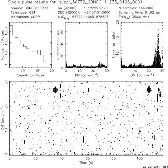
We used presto’s prepdata function to create a time series from the RFI-mitigated data at a DM of 0 pc cm-3, and prepsubband to create many de-dispersed time series over a range of DMs centered on the known DM of the pulsar. The DM spacing between time series and the downsampling factor used were calculated using presto’s DDplan.py, and are given in Table 1. We then used single_pulse_search.py to search each time series for pulses, recording any candidate single-pulse events with signal-to-noise ratios (S/Ns) greater than 5. We use an expanded list of boxcar widths in order to be sensitive to a variety of burst widths, and use a maximum boxcar width which corresponds to a pulse width of 100 ms.
We search over a range of DMs to discriminate astrophysical faint pulses from RFI, as the detected S/N of a single pulse from a pulsar will be decreased if the data are de-dispersed at an incorrect DM (Cordes and McLaughlin, 2003). The S/N is expected to be maximized at the DM of the pulsar, and fall off on either side; thus, even if the single-pulse search code repeatedly identifies the same pulse in multiple de-dispersed time series, the grouping of single-pulse events will be closely spaced in time, and the pulse can be identified by choosing the event with the highest S/N.
We observe variations in the DM that maximizes the S/N between single pulses, likely due to radiometer noise, as is evident by the distribution of single-pulse DMs in Figure 2. Thus, to avoid discarding real pulses, we accept single pulses with peak S/Ns at DMs within 10% of the fiducial DM, which is either determined by the peak DM of the brightest astrophysical pulse detected, or the DM measured through timing with integrated pulse profiles. In order to mitigate RFI which may be falsely flagged as a real pulse, a candidate is removed if there is a pulse at a DM of 0 pc cm-3 with a greater S/N within one pulse period of the candidate.
We created a template profile at each observing frequency by fitting a Gaussian template to the brightest single pulse, and measured a TOA for each pulse by cross-correlating it with this template profile. The errors on the TOA are approximated as the width of a bin divided by the signal-to-noise ratio of the pulse, as in McLaughlin et al. (2009). We visually inspected each pulse to confirm their astrophysical nature, removing pulses with baselines greatly affected by RFI.
II.2 TOA Generation– Integrated emission
These pulsars were all discovered through their single pulses, but in later follow-up observations, were sufficiently luminous to be detected by an FFT search at several observational epochs. In Karako-Argaman et al. (2015), the rotational period of J1126 was constrained using the time differences between detected single pulses, and the quoted rotational period of J0447 was a factor of four longer than the period we report here.
We used the FFT detections as the nominal rotational periods for each pulsar. After folding each observation, we combined the profiles for each detection into a high signal-to-noise (S/N) composite profile; the profiles for each pulsar are shown in the left panel of Figure 3. We then generated TOAs for each observation in which each pulsar was detected using the template profile and PRESTO’s get_TOAs.py; the TOA uncertainties were also reported by PRESTO. We generally used only one TOA for each observation except for a ‘phase-connection’ observation, an observation with a high-S/N detection which is closely spaced in time to other observations. An exemplary time-phase plot, integrated pulse profile, and set of single-pulse profiles are presented in Figure 4.
III Timing Solutions
We used the TEMPO2 software package to obtain all of the timing solutions, using the DE438 solar system ephemeris. We multiplied the uncertainty on each TOA so that the reduced value of the post-fit timing solution would be equal to one.
Since we were able to obtain TOAs at both 350 and 820 MHz for J0447, we also fit for DM in the process of pulsar timing, and the reported DM and error are obtained from the timing solution. For J0539 and J1126, we were only able to obtain TOAs at 350 MHz, and thus could not refine the DM measurements through timing. We attempted to fit for the DM by splitting the observing band into subbands and measuring a TOA within each subband, however, performing this analysis on the highest S/N observations for each pulsar did not yield more precise DM measurements than those previously constrained. Instead, we selected the 20 brightest pulses from our sample and took the weighted average of their PRESTO-reported DM, assuming a 5% uncertainty on the DM reported in the sections below.
III.1 PSR J0447–0432

The full timing solution for J0447 is given in Table 2, and the timing residuals are plotted in Figure 5. The derived sky positions and rotational parameters of the two methods are in agreement within two standard deviations.
The rotational period of J0447 was estimated through the single pulse arrival times in Karako-Argaman et al. (2015). According to the reported burst rate estimates, no more than three pulses would have been detected in a given observation. The use of the greatest common denominator between pulse times as an estimate for a RRAT’s rotational period can often lead to a period estimate greater than the true rotational period, and simulations by Cui et al. (2017) show that the probability of determining an incorrect period from three pulses in an observation is roughly 37%; thus, the overestimated period for J0447 is not surprising.
There are five epochs with single pulse TOAs but no integrated TOA in the timing solutions, and one epoch with an integrated TOA but no single pulse TOAs. Three of the epochs with only single pulse TOAs were significantly corrupted by RFI so that an integrated TOA was not obtainable, and the other two observations were shorter than ten minutes long and yielded a signal that was too weak to reliably measure an integrated TOA. The observation with an integrated TOA but no single pulse TOAs was at 350 MHz and there were no single pulses with S/N 5 detected by PRESTO; the lack of bright single pulses at 350 MHz is discussed further in Section IV.1.
| Integrated Timing | Single Pulse Timing | |
|---|---|---|
| Right ascension (J2000) | ||
| Declination (J2000) | ||
| Spin frequency (Hz) | 1.82798530966(7) | 1.82798530954(9) |
| Spin frequency derivative (Hz s-1) | –1.91(1) | –1.930(6) |
| Dispersion measure (pc cm-3) | 29.85(5) | 29.75(1) |
| Spin period, (s) | 0.54705034812(2) | 0.54705034815(1) |
| Spin-down rate, (s s-1) | 5.72(3) | 5.78(2) |
| Surface magnetic field, B ( G) | 0.18 | |
| Spin-down luminosity, ( erg s-1) | 1.4 | |
| Characteristic age, (Myr) | 150 | |
| DM distance (kpc) (NE2001) | 1.3 | |
| DM distance (kpc) (YMW16) | 0.7 | |
| Data span (yr) | 3.14 | |
| Start epoch (MJD) | 56758 | |
| End epoch (MJD) | 57907 | |
| Timing epoch | 57815 | |
| Number of observations | 16 | 21 |
| Number of TOAs | 23 | 512 |
| Post-fit residual RMS (s) | 596 | 1549 |
| Reduced chi-squared | 2.4 | 20.2 |
Note. — Timing parameters for the integrated and single-pulse timing models for PSR J0447–0432. 1 error bars are denoted with parenthesis on the last significant digit. The uncertainties have been adjusted with the MODE 1 setting in tempo2 so that the final solution has a reduced chi-squared of one. Both timing models use the DE438 solar system ephemeris and are referenced to the TT(TAI) time standard.
III.2 PSR J0539+0010


The full timing solution for J0539 is given in Table 3, and the timing residuals are plotted in Figure 6. The derived rotational parameters of the two methods are in agreement within two standard deviations.
The integrated profile of J0539 consistently shows a double-peaked shape across observational epochs. The residuals of the single-pulse TOAs cluster within two main bands, with approximately 17% of pulse residuals falling between the two peaks, and the remainder distributed equally across both bands. The left panel of Figure 7 shows the distribution of the residuals of the single-pulse TOAs, using the best-fit timing solution derived from these TOAs. The bands are centered roughly at pulse phases of 0.025, equivalent to ms from the center of the profile.
Pulsar timing methodology is based on the assumption that the pulse originates from the same rotational phase every time. In order to obtain a single-pulse timing solution with lower uncertainties, we first wanted to find the optimal amount by which to shift the TOAs in each band to align the TOAs to a single peak, as in Lyne et al. (2009). We defined the early and late bands as being composed of TOAs with residuals with absolute values in phase, and searched 30 offsets between pulse phases of 0.02 and 0.03 for each band, creating a set of TOAs with the early- and late-band TOAs shifted by the corresponding amount. We chose the offsets corresponding to the set of TOAs which, when run through tempo2, yielded the timing solution with the lowest RMS residual. This resulted in offsets of 34.9 ms for the early band and 32.5 ms for the late band. The RMS residual on the solution decreased from 27.2 ms to 7.2 ms after the TOAs were adjusted, and the uncertainties on the parameters by similar factors.
There are three RFI-impacted epochs with single pulse TOAs but no integrated TOA in the timing solutions, and there is one epoch with an integrated TOA but no single pulse TOAs, as no single pulses with S/N 7 were detected by PRESTO, and the few single pulses with 5 S/N 7 were not suitably bright for a reliable TOA measurement.
| Integrated Timing | Single Pulse Timing | |
|---|---|---|
| Right ascension (J2000) | ||
| Declination (J2000) | ||
| Spin frequency (Hz) | 0.84935705136(5) | 0.84935705146(4) |
| Spin frequency derivative (Hz s-1) | –2.504(5) | –2.509(3) |
| Dispersion measure (pc cm-3) | 48.46(2) | |
| Spin period, (s) | 1.17736115618(7) | 1.17736115604(6) |
| Spin-down rate, (s s-1) | 3.470(7) | 3.478(5) |
| Surface magnetic field, B ( G) | 2.0 | |
| Spin-down luminosity, ( erg s-1) | 8.4 | |
| Characteristic age, (Myr) | 5.4 | |
| DM distance (kpc) (NE2001) | 2.0 | |
| DM distance (kpc) (YMW16) | 1.4 | |
| Data span (yr) | 1.82 | |
| Start epoch (MJD) | 58109 | |
| End epoch (MJD) | 58772 | |
| Timing epoch | 58384 | |
| Number of observations | 17 | 19 |
| Number of TOAs | 29 | 315 |
| RMS post-fit residuals (s) | 1950 | 716 |
| Reduced chi-squared | 0.64 | 61 |
Note. — Timing parameters for the integrated and single-pulse timing models for PSR J0539+0010. 1 error bars are denoted with parenthesis on the last significant digit. The uncertainties have been adjusted with the MODE 1 setting in tempo2 so that the final solution has a reduced chi-squared of one. Both timing models use the DE438 solar system ephemeris and are referenced to the TT(TAI) time standard.
III.3 PSR J1126–2739

The full timing solution for J1126 is given in Table 4, and the timing residuals are plotted in Figure 8. The rotational parameters of the two methods are in agreement within two standard deviations, and the sky positions are in agreement within 2.5 standard deviations.
There are two RFI-impacted epochs with single pulse TOAs but no integrated TOA in the timing solutions, and two epochs with an integrated TOA but no single pulse TOAs, as no single pulses with S/N 7 were detected by PRESTO, and the few single pulses with 5 S/N 7 were not suitably bright for a reliable TOA measurement.
| Integrated Timing | Single-Pulse Timing | |
|---|---|---|
| Right ascension (J2000) | ||
| Declination (J2000) | ||
| Spin frequency (Hz) | 2.79207295863(4) | 2.79207295872(3) |
| Spin frequency derivative (Hz s-1) | –7.921(2) | –7.920(1) |
| Dispersion measure (pc cm-3) | 26.86(1) | |
| Spin period, (s) | 0.358156830004(4) | 0.358156829992(4) |
| Spin-down rate, (s s-1) | 1.0160(2) | 1.0159(2) |
| Surface magnetic field, B ( G) | 0.610 | |
| Spin-down luminosity, ( erg s-1) | 87.3 | |
| Characteristic age, (Myr) | 5.6 | |
| DM distance (kpc) (NE2001) | 1.1 | |
| DM distance (kpc) (YMW16) | 0.4 | |
| Data span (yr) | 4.7 | |
| Start epoch (MJD) | 57153 | |
| End epoch (MJD) | 58874 | |
| Timing epoch | 58013 | |
| Number of observations | 19 | 21 |
| Number of TOAs | 49 | 237 |
| RMS post-fit residuals (s) | 1100 | 1742 |
| Reduced chi-squared | 1.91 | 54.8 |
Note. — Timing parameters for the integrated and single-pulse timing models for PSR J1126–2739. 1 error bars are denoted with parenthesis on the last significant digit. The uncertainties have been adjusted with the MODE 1 setting in tempo2 so that the final solution has a reduced chi-squared of one. Both timing models use the DE438 solar system ephemeris and are referenced to the TT(TAI) time standard.
IV Emission Properties
IV.1 Pulse Rates

The rate of detected pulses within each observation, defined as the number of single pulse TOAs divided by the observation length, is shown for all three pulsars in Figure 9. J0447 has consistently higher pulse rates at 820 MHz (mean rate of 132 pulses hr-1) compared to 350 MHz (mean rate of 28 pulses hr1), which is also clear from the single-pulse residuals in Figure 5. The predicted scattering timescales are roughly 0.4 and 730 s at 820 and 350 MHz respectively, so the signal is not scattered out at lower frequencies, and we do not see strong scattering tails in the profiles of this pulsar at 350 MHz (e.g. Figure 3).
At 350 MHz, the system temperature is higher, and the effective bandwidth is roughly one third of that of the 820 MHz receiver. Using the radiometer equation, a detection threshold S/N of 6 implies a single pulse flux detection threshold of 8 mJy at 820 MHz, and 20 mJy at 350 MHz. We also used the radiometer equation to estimate the mean flux of J0447 in each observation, finding an average flux of mJy at 820 MHz and mJy at 350 MHz, where the error bars are the standard deviations of all of the flux measurements at that frequency.
Assuming that J0447 follows a simple spectral power law with the average pulsar spectral index of (Jankowski et al., 2018), the mean flux at 350 MHz would be roughly four times higher than that at 820 MHz, and we would expect more single pulses exceeding the detection threshold at 350 MHz than at 820. Conversely, the detected pulse rate at 820 MHz is on average 4.5 times greater than the pulse rate at 350 MHz, though the time-averaged fluxes are very similar between the two frequencies. We thus conclude that there are fewer, though brighter, detected single pulses at 350 MHz compared to at 820 MHz where the single-pulse detection threshold is lower.
IV.2 Wait Times and Pulse Clustering

| PSR | (hr-1) | (hr-1) | FP | |
|---|---|---|---|---|
| J0447–0432 | ||||
| J0539+0010 | ||||
| J1126–2739 |
Note. — The wait time distribution fit results: is the Poissonian burst rate, the Weibull burst rate, and the Weibull clustering parameter. The final column denotes the probability that the improvement to the fit from the Weibull distribution is due to random chance. 1- error bars are denoted.
We used the measured arrival times of each pulse to create a wait time distribution, excluding any wait times between observations due to the sporadic cadence of our observations. We fit Poisson and Weibull distributions to each distribution using scipy.optimize.curve_fit and report the results of each fit in Table 5. The number of bins in each distribution were chosen using the Freedman Diaconis estimator. The wait times, in units of pulsar rotations, are shown in Figure 10 along with the fitted statistical distributions.
The distribution of wait times from J0447 shows slight evidence of a secondary peak of wait times centered at around 75 periods, although the inclusion of a Maxwell-Boltzmann or Gaussian component did not yield a statistically significant improvement in the quality of the fit. Similar secondary ‘bumps’ in the wait time distribution were observed in PSRs J1317–5759 and J1819–1458, with increased wait times at 25 pulse periods, although no statistical distribution was able to fully describe the bumps in the distribution, likely due to the complex nature of the wait time distributions (Shapiro-Albert et al., 2018).
Since only the TOAs from the timing analysis were used to calculate the wait times, low-luminosity pulses would not be considered, potentially introducing a bias towards longer wait times. Additionally, excising rotations corrupted by RFI could cause astrophysical pulses to be excised, artificially increasing the reported wait times. To measure the effect of the long-wait tails on the distribution fits, we re-ran the wait time analysis only on wait times shorter than a given threshold; cutoff thresholds of 200, 250, and 500 rotational periods each yielded results in agreement with those reported in Table 5. Overall, we find that the Weibull distribution with is preferred for all three pulsars, indicating that pulse clustering on short timescales is present.
We performed a statistical F-test to compare the goodness of fit of the two distributions, and determine if adding the extra parameter in fitting the Weibull distribution makes a statistically significant improvement to the fit. The F-test returns a statistic which we use to determine the probability that the improvement to the fit is due to random chance. These false alarm probabilities are presented in the final column of Table 5, and indicate that the wait times from J0539 are much better fit by a Weibull distribution, and the same is true to a lesser extent for J0447. We conclude that significant amounts of pulse clustering are present in the emission from PSRs J0447 and J0539, and that the pulse clustering model may be preferred for PSR J1126, but with lower certainty.
IV.3 Pulse Energy Distributions

We determined on-pulse and off-pulse regions for each pulsar by visible inspection of their time-phase plots. For each pulse, the on-pulse energy and off-pulse standard deviation were calculated, and normalized by the average on-pulse energy of all rotations from that observation. The resulting distributions are shown in Figure 11 (left panel). In nulling pulsars of sufficient brightness such a distribution naturally separates into two distinct components (see, e.g., van Leeuwen et al., 2002), allowing an unambiguous distinction between pulses with and without emission. In these three cases, however, the energy distributions are continuous. We choose as the boundary, and study the pulse energy distribution of pulses exceeding that. The pulse energies of all these pulses with are next plotted for each pulsar in the right panel of Figure 11, alongside the best-fit log-normal and power law distributions fit using scipy.optimize.curve_fit. A combined log-normal and power-law distribution was also tested, but led to worse fits for all three pulsars, so we do not plot them.
The fit results indicate that a power-law distribution is preferred over a log-normal energy distribution for all three pulsars in this sample. A power law tail in the energy distribution implies the presence of giant pulses; however, giant pulses from the Crab pulsar and others are several orders of magnitude brighter than the average pulsed flux. We do not see such a pronounced increase in pulse energy in the brightest pulses from this sample, with only one pulse from J1126 being greater than ten times more energetic than the average pulse energy. The lack of exceptionally bright pulses leads us to conclude that the emission mechanisms are more similar to the standard pulsar model, as opposed to giant pulse emission, despite the slight preference for power law distributions. We also examined the pulse energies as a function of the wait time between detected pulses finding no correlation, suggesting that energy is not being stored up between pulses.
IV.4 Weak Emission

Characterization of the emission properties of many pulsars by the FAST GPPS survey grouped them into three loose groups: the majority of RRATs are “normal” pulsars with occasional bright pulses, some are extreme nullers, and some show very few bright pulses with no weak emission (Zhou et al., 2023). To determine the emission patterns of these pulsars, we used the de-dispersed data cubes to create time-phase plots and total integrated profiles for each observation. We then extracted all subintegrations with signal-to-noise ratios , and created profiles exclusively from those pulses, as well as a “noise” profile consisting only of subintegrations with , which are shown in Figure 12. While the majority of the emission comes from the sporadic, bright pulses, each pulsar shows evidence of sub-threshold emission, particularly J0447.
V Discussion
V.1 Timing


We successfully obtained phase-connected timing solutions for these three pulsars using the standard method of integrating the emission by folding the data, as well as by measuring TOAs for each detected single pulse. The independently obtained sets of TOAs provide an opportunity to cross-reference the derived timing parameters between solutions, and evaluate the accuracy and precision of the two timing methods.
For all three pulsars, the single-pulse timing solutions have larger RMS post-fit residuals and larger reduced chi-squared values999Using the MODE 1 setting in tempo2, the uncertainties on the TOAs were multiplied by a factor so that the reduced chi-squared values of the final solutions would be one., suggesting that these timing models fit the observed TOAs less accurately, and that there would be more uncertainty in the derived parameters making up the timing model. However, the timing-derived parameters have error bars of similar sizes and are generally in good agreement between the two timing methods for all three pulsars. To visualize this, we have plotted the period and period derivative (Figure 13) and the sky positions (Figure 14) returned by the best-fit timing models for each pulsar using both methods, as well as the error bars on each. All of the parameters are in agreement between the two solutions within two standard deviations. This indicates that the timing solutions are of comparable accuracy. The error bars on the parameters from single-pulse timing are consistently less than or equal to the error bars on the same parameters from the integrated timing solution; the greater number of TOAs and detection of single pulses on epochs without folding detections likely allowed for more accurate constraints on these parameters.
The two methods studied here yield spin parameters and sky positions with similar-sized error bars, yet the RMS and reduced chi squared () of the single-pulse solutions are significantly higher, due to the large number of TOAs scattered across a larger pulse phase envelope. To perform the fits, tempo2 first measures the residual of each pulse, the difference between the predicted and observed arrival times based on the provided pre-fit timing model. tempo2 uses a weighted least-squares algorithm to minimize the chi-squared value:
| (1) |
Here, is the residual of the TOA, is the uncertainty on the TOA, and the sum is performed over all of the TOAs used in the timing model (Hobbs et al., 2006).
Under this formulation, a clear disparity arises between the two methods. Using folding, many single pulses which may arrive within a larger pulse envelope are averaged together into one pulse profile. On the other hand, each detected pulse may peak anywhere within a window that encompasses a few percent of the total rotational period of the source. These variations are intrinsic to the pulsar emission process, however, when these single-pulse TOAs are used to calculate a timing model, the large number of pulses with large residuals will yield a calculation of and the root-mean-square residual value which are much higher than the corresponding values in the integrated timing solution.
Hybrid timing models, formed from a combination of integrated and single-pulse TOAs, may be used for pulsars with infrequent observational cadences, or small amounts of TOAs that make timing difficult. Epochs with single-pulse TOAs but no measurable integrated profile are common in the RRAT-like emission regime, but we also have observations with integrated TOAs but no single-pulse TOAs. These are typically short observations, with a small number of detected single pulses with S/N , too dim to return a useful TOA measurement. While a hybrid method would be useful for extending timing baselines where necessary, the different uncertainty calculations for different types of TOAs would require more careful analysis for the derived timing parameters and their errors.
V.2 Pulse Jitter
On short timescales, the uncertainty in TOA measurements are dominated by radiometer noise, jitter noise, and scintillation noise (Lam et al., 2019). Radiometer noise typically dominates low S/N observations, as the limited sensitivity impacts the effectiveness of template matching. The single pulses from all pulsars vary stochastically in both shape and arrival phase, contributing an excess noise component known as pulse jitter. As observational sensitivity increases, pulse jitter is expected to become the dominant source of noise, especially for millisecond pulsars (Lam et al. 2019; Miao et al. 2023; Wang et al. 2024). Previous estimates of the jitter-induced uncertainty have come either from cross-correlation of the TOA errors from different frequency bands (Miao et al., 2023), or by comparing the observed variance of the TOAs with the variance of idealized simulated datasets for each pulsar (Parthasarathy et al. 2021; Wang et al. 2024), both of which are outside the scope of this work.
For each observational epoch, we calculate the mean TOA error of the integrated TOAs, and compare this to the RMS of all the single-pulse TOAs from that epoch. We only examined observations with more than five single-pulse TOAs, and calculated the ratio of the single-pulse RMS over the mean integrated TOA error. We find that the ratio varies between five and 25 for almost all of our observational epochs; averaging over all of the observations yields mean ratios of 19, 13, and eight for PSRs J0447, J0539, and J1126 respectively.
V.3 Single-Pulse Properties
In this work, we fitted log-normal and power-law functions to the normalized pulse energy distribution and found that power law distributions are preferred for two of the pulsars. Despite this, we see no evidence of giant pulses with energies times the average pulse energy, and all three pulsars show evidence of weak emission outside of the bright pulses. We conclude that the emission mechanisms at play here are fundamentally the same as for standard pulsars.
We also analyzed the wait time distributions of all three pulsars and found that Weibull distributions were preferred, implying moderate amounts of pulse clustering in time. While some pulses arrive consecutively, we do not exclusively observe “active” periods of several consecutive pulses followed by periods with no emission, and we are able to detect weak emission outside the bright pulses for each pulsar, leading us to conclude that these pulsars are not just extremely nulling pulsars.
VI Conclusion
We report phase-connected timing solutions for three radio pulsars discovered at 350 MHz with the GBNCC and GBT 350-MHz drift scan surveys. Two of these pulsars were initially published as RRATs due to their discovery through single-pulse detection pipelines, but in subsequent observations, were sufficiently bright to form integrated pulse profiles and measure times of arrival. We formed two distinct timing models from different sets of TOAs: the integrated pulse profiles, and the arrival times of all detected single pulses. The best-fit sky coordinates, period, and period derivative are in agreement within standard deviations. The error bars on the parameters are of similar size between the two timing models, although the reported RMS error of the single-pulse solutions are much higher for two of the pulsars owing to the large number of single pulses falling within a relatively wide phase envelope.
The wait-time distributions of each pulsar are better fit to a model in which pulses tend to be clustered together in time, suggesting that the pulses do not occur randomly or independently. The energy distributions tend to prefer power law distributions, although no pulses meet the S/N 10 threshold as a loose definition of “giant pulses”, and the presence of weak emission outside the bright pulses indicates that these are weaker pulsars with sparse bright pulses, as is the case for many RRATs as they are observed with the next generation of more sensitive radio telescopes. This work shows the applicability of multiple TOA generation methods, and highlights the variety of emission characteristics of pulsars under the RRAT umbrella.
References
- Radio pulsar sub-populations (II): The mysterious RRATs. Journal of Astrophysics and Astronomy 43 (2), pp. 75. External Links: Document, 2201.00295 Cited by: §I.
- The Green Bank North Celestial Cap Pulsar Survey. IV. Four New Timing Solutions. ApJ 875 (1), pp. 19. External Links: Document, 1903.03543 Cited by: §II.
- The Astropy Project: Sustaining and Growing a Community-oriented Open-source Project and the Latest Major Release (v5.0) of the Core Package. ApJ 935 (2), pp. 167. External Links: Document, 2206.14220 Cited by: Multi-Method Timing of Transient Radio Pulsars with the GBT350 and GBNCC Surveys.
- MeerTRAP: 12 Galactic fast transients detected in a real-time, commensal MeerKAT survey. MNRAS 512 (1), pp. 1483–1498. External Links: Document, 2203.00557 Cited by: §I.
- The Green Bank Telescope 350 MHz Drift-scan survey. I. Survey Observations and the Discovery of 13 Pulsars. ApJ 763 (2), pp. 80. External Links: Document, 1209.4293 Cited by: §II.
- The millisecond radio sky: transients from a blind single-pulse search. MNRAS 402 (2), pp. 855–866. External Links: Document, 0911.1790 Cited by: §I, §I.
- The High Time Resolution Universe Pulsar Survey - V. Single-pulse energetics and modulation properties of 315 pulsars. MNRAS 423 (2), pp. 1351–1367. External Links: Document, 1203.6068 Cited by: §I.
- An investigation of pulsar searching techniques with the fast folding algorithm. MNRAS 468 (2), pp. 1994–2010. External Links: Document, 1703.05581 Cited by: §I.
- Searches for Fast Radio Transients. ApJ 596 (2), pp. 1142–1154. External Links: Document, astro-ph/0304364 Cited by: §II.1.
- Timing Solution and Single-pulse Properties for Eight Rotating Radio Transients. ApJ 840 (1), pp. 5. External Links: Document, 1706.08412 Cited by: §I, §III.1.
- A Statistical Analysis of Crab Pulsar Giant Pulse Rates. ApJ 973 (2), pp. 87. External Links: Document, 2407.15996 Cited by: §I.
- Launching GUPPI: the Green Bank Ultimate Pulsar Processing Instrument. In Advanced Software and Control for Astronomy II, A. Bridger and N. M. Radziwill (Eds.), Society of Photo-Optical Instrumentation Engineers (SPIE) Conference Series, Vol. 7019, pp. 70191D. External Links: Document Cited by: §II.
- RRAT J2325–0530: A Rotating Radio Transient with an Atypical Waiting-time Distribution. ApJ 991 (2), pp. 201. External Links: Document, 2508.17657 Cited by: §I, §I.
- Confidence Limits for Small Numbers of Events in Astrophysical Data. ApJ 303, pp. 336. External Links: Document Cited by: Figure 9.
- Array programming with NumPy. Nature 585 (7825), pp. 357–362. External Links: Document, Link Cited by: Multi-Method Timing of Transient Radio Pulsars with the GBT350 and GBNCC Surveys.
- TEMPO2, a new pulsar-timing package - I. An overview. MNRAS 369 (2), pp. 655–672. External Links: Document, astro-ph/0603381 Cited by: §V.1, Multi-Method Timing of Transient Radio Pulsars with the GBT350 and GBNCC Surveys.
- Matplotlib: a 2d graphics environment. Computing in Science & Engineering 9 (3), pp. 90–95. External Links: Document Cited by: Multi-Method Timing of Transient Radio Pulsars with the GBT350 and GBNCC Surveys.
- Spectral properties of 441 radio pulsars. MNRAS 473 (4), pp. 4436–4458. External Links: Document, 1709.08864 Cited by: §IV.1.
- Discovery and Follow-up of Rotating Radio Transients with the Green Bank and LOFAR Telescopes. ApJ 809 (1), pp. 67. External Links: Document, 1503.05170 Cited by: §II.2, §II, §II, §III.1.
- Giant pulses from the Crab pulsar. A wide-band study. A&A 515, pp. A36. External Links: Document, 1004.2803 Cited by: §I.
- The Green Bank Northern Celestial Cap Pulsar Survey. II. The Discovery and Timing of 10 Pulsars. ApJ 857 (2), pp. 131. External Links: Document, 1803.03587 Cited by: §II.
- On the birthrates of Galactic neutron stars. MNRAS 391 (4), pp. 2009–2016. External Links: Document, 0810.1512 Cited by: §I.
- Rotating radio transients. Bulletin of the Astronomical Society of India 39 (3), pp. 333–352. External Links: Document, 1109.6896 Cited by: §I.
- The NANOGrav 12.5 yr Data Set: The Frequency Dependence of Pulse Jitter in Precision Millisecond Pulsars. ApJ 872 (2), pp. 193. External Links: Document, 1809.03058 Cited by: §I, §V.2.
- FAST in Space: Considerations for a Multibeam, Multipurpose Survey Using China’s 500-m Aperture Spherical Radio Telescope (FAST). IEEE Microwave Magazine 19 (3), pp. 112–119. External Links: Document, 1802.03709 Cited by: §II.
- Handbook of Pulsar Astronomy. Cited by: §I.
- The Green Bank Telescope 350 MHz Drift-scan Survey II: Data Analysis and the Timing of 10 New Pulsars, Including a Relativistic Binary. ApJ 763 (2), pp. 81. External Links: Document, 1209.4296 Cited by: §II.
- The Green Bank North Celestial Cap Pulsar Survey. III. 45 New Pulsar Timing Solutions. ApJ 859 (2), pp. 93. External Links: Document, 1805.04951 Cited by: §II.
- Unusual glitch activity in the RRAT J1819-1458: an exhausted magnetar?. MNRAS 400 (3), pp. 1439–1444. External Links: Document, 0909.1165 Cited by: §III.2.
- The Australia Telescope National Facility Pulsar Catalogue. AJ 129 (4), pp. 1993–2006. External Links: Document, astro-ph/0412641 Cited by: §I.
- The Green Bank North Celestial Cap Pulsar Survey. V. Pulsar Census and Survey Sensitivity. ApJ 892 (2), pp. 76. External Links: Document, 1909.11109 Cited by: §II.
- Timing observations of rotating radio transients. MNRAS 400 (3), pp. 1431–1438. External Links: Document, 0908.3813 Cited by: §I, §II.1.
- Transient radio bursts from rotating neutron stars. Nature 439 (7078), pp. 817–820. External Links: Document, astro-ph/0511587 Cited by: §I.
- Variability, polarimetry, and timing properties of single pulses from PSR J2222-0137 using FAST. MNRAS 526 (2), pp. 2156–2166. External Links: Document, 2308.10683 Cited by: §V.2.
- A Giant Sample of Giant Pulses from the Crab Pulsar. ApJ 760 (1), pp. 64. External Links: Document, 1210.0452 Cited by: §I.
- A study of single pulses in the Parkes Multibeam Pulsar Survey. MNRAS 479 (4), pp. 5413–5422. External Links: Document, 1807.00143 Cited by: §I.
- On the non-Poissonian repetition pattern of FRB121102. MNRAS 475 (4), pp. 5109–5115. External Links: Document, 1705.04881 Cited by: §I.
- The Implementation of a Fast-folding Pipeline for Long-period Pulsar Searching in the PALFA Survey. ApJ 861 (1), pp. 44. External Links: Document, 1805.08247 Cited by: §I.
- Measurements of pulse jitter and single-pulse variability in millisecond pulsars using MeerKAT. MNRAS 502 (1), pp. 407–422. External Links: Document, 2101.08531 Cited by: §V.2.
- PyGDSM: Python interface to Global Diffuse Sky Models. Note: Astrophysics Source Code Library, record ascl:1603.013 Cited by: Multi-Method Timing of Transient Radio Pulsars with the GBT350 and GBNCC Surveys.
- PRESTO: PulsaR Exploration and Search TOolkit Note: Astrophysics Source Code Library, record ascl:1107.017 External Links: 1107.017 Cited by: §II, Multi-Method Timing of Transient Radio Pulsars with the GBT350 and GBNCC Surveys.
- Radio Properties of Rotating Radio Transients: Single-pulse Spectral and Wait-time Analyses. ApJ 866 (2), pp. 152. External Links: Document, 1809.06729 Cited by: §I, §IV.2.
- The Green Bank Northern Celestial Cap Pulsar Survey. I. Survey Description, Data Analysis, and Initial Results. ApJ 791 (1), pp. 67. External Links: Document, 1406.5214 Cited by: §II.
- A single pulse study of PSR J1752+2359. Research in Astronomy and Astrophysics 21 (9), pp. 240. External Links: Document Cited by: §I.
- Null-induced mode changes in PSR B0809+74. A&A 387, pp. 169–178. External Links: Document, astro-ph/0202477 Cited by: §IV.3.
- LOFAR radio search for single and periodic pulses from M 31. A&A 634, pp. A3. External Links: Document, 1911.11228 Cited by: §I.
- SciPy 1.0: Fundamental Algorithms for Scientific Computing in Python. Nature Methods 17, pp. 261–272. External Links: Document Cited by: Multi-Method Timing of Transient Radio Pulsars with the GBT350 and GBNCC Surveys.
- Pulsar nulling and mode changing. MNRAS 377 (3), pp. 1383–1392. External Links: Document, astro-ph/0703241 Cited by: §I.
- Pulse Jitter and Single-pulse Variability in Millisecond Pulsars. ApJ 964 (1), pp. 6. External Links: Document, 2401.12426 Cited by: §V.2.
- seaborn: statistical data visualization. The Journal of Open Source Software 6 (60), pp. 3021. External Links: Document Cited by: Multi-Method Timing of Transient Radio Pulsars with the GBT350 and GBNCC Surveys.
- The FAST Galactic Plane Pulsar Snapshot Survey. II. Discovery of 76 Galactic Rotating Radio Transients and the Enigma of RRATs. Research in Astronomy and Astrophysics 23 (10), pp. 104001. External Links: Document, 2303.17279 Cited by: §I, §I, §I, §IV.4.