[2]\fnmZhiliang \surDeng

1]\orgdivSchool of Mathematics, \orgnameSouthwest Jiaotong University, \orgaddress\streetXi’an Road, \cityChengdu, \postcode611756, \stateSichuan, \countryChina

[2]\orgdivSchool of Mathematical Science, \orgnameUniversity of Electronic Science and Technology of China, \orgaddress\streetXiyuan Ave, \cityChengdu, \postcode611731, \stateSichuan, \countryChina

Hamiltonian Monte Carlo from $q$ -deformed phase-space mechanics

\fnmXiaomei \surYang yangxiaomath@swjtu.edu.cn dengzhl@uestc.edu.cn [ *

Abstract

Hamiltonian Monte Carlo (HMC) constructs Markov transitions by combining Hamiltonian dynamics with a Metropolis correction. This paper develops a $q$ -deformed HMC framework motivated by $q$ -deformed phase-space mechanics. Starting from a Lagrangian formulation, we derive the corresponding $q$ -Hamiltonian equations and show the formal invariance of the associated $q$ -symplectic form. This provides a geometric origin for the proposed $q$ -HMC dynamics rather than treating it as an ad hoc finite-difference modification. To obtain a computable sampler for ordinary target distributions, we realize the formal $q$ -differential operators through Jackson-type differences and construct a Metropolis-adjusted $q$ -Hamiltonian proposal. The resulting transition reduces to classical HMC as $q\to 1$ , satisfies detailed balance under the Metropolis correction, and admits sufficient nondegeneracy conditions for irreducibility of the marginal position chain. Numerical experiments on benchmark targets, positive-scale black-box targets, a mixed positive/signed target, and a PDE-based Bayesian inverse problem show that the $q$ -Jackson force acts as a relative perturbation mechanism in the original variables. It avoids the domain violations and scale mismatch that can occur with raw additive finite differences, while tracking exact-gradient, adjoint-force, or carefully scaled finite-difference benchmarks when these are available.

keywords:

Hamiltonian Monte Carlo,

q

-calculus, Jackson derivative, noncommutative geometry, finite-difference force

1 Introduction

Hamiltonian Monte Carlo (HMC) is a powerful Markov chain Monte Carlo method for sampling from probability distributions of the form

\displaystyle\pi(x)\propto\exp[-U(x)],

(1)

where $U(x)$ is the potential function. By augmenting the parameter $x$ with an auxiliary momentum variable $p$ , HMC constructs proposals through Hamiltonian dynamics in the extended phase space. Compared with random-walk-type methods, HMC can generate distant proposals while maintaining high acceptance probabilities, and has become a standard tool in Bayesian computation, statistical machine learning, and scientific computing [Betancourt2017, Bishop2006, Bou-Rabee2020, Duane1987, Durmus2020, Livingstone2019, Mackay2003, Neal1995, Neal2011].

The performance of HMC is closely tied to the geometric structure of the underlying Hamiltonian system. In the classical setting, the Hamiltonian flow preserves the symplectic form and the phase-space volume, which provides the foundation for stable long-distance proposals. In practical computations, however, the continuous Hamiltonian flow must be approximated by a numerical integrator, and the resulting proposal must be corrected by a Metropolis step. This geometric viewpoint has motivated a variety of extensions of HMC, including modified or shadow Hamiltonian methods [Akhmatskaya2008, Radivojevic2020, Heide2021], alternative choices of kinetic energy [Livingstone2019_b, Lu2017], non-Euclidean or Riemannian-manifold metrics [Betancourt2013, Girolami2011], and other structure-preserving proposal mechanisms based on symplectic or volume-preserving discretizations [Afshar2015, Chao2015, Neal2011]. In this paper, we pursue a different direction: we study a $q$ -deformed analogue of Hamiltonian dynamics and use it to construct a corresponding $q$ -HMC sampler.

The motivation comes from $q$ -deformed mechanics on $q$ -commutative spaces. In $q$ -calculus, ordinary derivatives are replaced by Jackson-type finite differences, and the underlying phase-space algebra is modified by $q$ -commutation relations. Such structures have been studied in the context of $q$ -deformed quantum mechanics and non-commutative geometry [Bardek2000, Cerchiai1999, Hinterding1999, Iida1992, Wess1990]. In particular, Lavagno et al. [Lavagno2006] formulated a $q$ -deformed Hamiltonian system through a $q$ -Poisson bracket. These constructions suggest a natural question: can one build an HMC-type sampling method by replacing the classical Hamiltonian dynamics with a computable $q$ -deformed Hamiltonian dynamics?

We answer this question by developing a geometric $q$ -analogue of HMC. Starting from a Lagrangian formulation, we derive the $q$ -Hamiltonian equations associated with the $q$ -commutative phase space. We then prove the invariance of the corresponding $q$ -symplectic form under the formal $q$ -Hamiltonian flow. This result may be viewed as a $q$ -analogue of the classical symplectic invariance and Liouville theorem, formulated within the $q$ -deformed differential calculus. Since the formal operator-valued dynamics is not directly suitable for numerical simulation, we subsequently introduce a computable realization based on Jackson derivatives. The resulting deterministic proposal mechanism reduces to classical Hamiltonian dynamics as $q\to 1$ , while for $q\neq 1$ it replaces ordinary derivatives by $q$ -Jackson finite differences. Because the computable $q$ -deformed proposal is not, in general, a canonical Hamiltonian flow in the ordinary Euclidean phase space, its validity as an MCMC transition must be established through a Metropolis correction. We therefore construct a Metropolis-corrected $q$ -HMC algorithm and prove that the resulting Markov transition satisfies the detailed balance condition with respect to the target distribution.

In addition to the general geometric construction, the $q$ -Jackson force has a useful computational interpretation. It perturbs variables multiplicatively rather than additively. This feature is not restricted to a single class of targets, but it becomes especially transparent for positive variables. If $s>0$ and $y=\log s$ , then the symmetric multiplicative perturbations $s\mapsto e^{\delta/2}s$ and $s\mapsto e^{-\delta/2}s$ , with $\delta=|\log q|$ , correspond to centered perturbations $y\mapsto y\pm\delta/2$ in the log-coordinate. Thus, for positive black-box targets, the $q$ -Jackson force can be interpreted as a multiplicative implementation of a log-coordinate finite difference. This observation provides one concrete regime in which the $q$ -analogue proposal exhibits a visible practical advantage.

The numerical experiments are organized to examine both the validity and the computational behavior of the proposed method. We compare $q$ -HMC with classical HMC, raw additive finite-difference HMC, and log-coordinate finite-difference HMC. The experiments show that the proposed method is a valid HMC-type sampler and that, in positive-scale and multiscale black-box targets, the $q$ -Jackson force can avoid the instability caused by raw additive perturbations. In these cases, $q$ -HMC closely tracks log-coordinate finite-difference HMC and the exact-gradient benchmark, while raw additive finite differences may produce large force errors, large Hamiltonian errors, and poor acceptance rates.

The rest of the paper is organized as follows. Section 2 derives the $q$ -deformed Hamiltonian system and proves the invariance of the associated $q$ -symplectic form. Subsequently, a computable $q$ -Hamiltonian system is presented via the $q$ -Jackson derivative. Section 3 introduces the $q$ -HMC algorithm and establishes its validity as a Markov chain Monte Carlo method, including detailed balance and irreducibility conditions. Section 4 presents the computational interpretation and numerical behavior of the $q$ -Jackson force. In particular, it explains its relation to finite-difference approximations and demonstrates its scale-consistency advantage for positive, multiscale, and mixed-coordinate black-box targets. Section 5 concludes the paper.

2 A $q$ -Analogue of Hamiltonian Dynamics

This section develops the geometric $q$ -analogue of Hamiltonian dynamics that will later serve as the basis for the proposed sampler. We first recall the $q$ -covariant differential structure on the quantum plane, derive the corresponding $q$ -Hamiltonian equations from a Lagrangian formulation, and prove the invariance of the associated $q$ -symplectic form. The same $q$ -Hamiltonian system was introduced in [Lavagno2006] through a $q$ -Poisson bracket; the present derivation provides a complementary Lagrangian viewpoint and makes the underlying symplectic structure explicit. These results are formulated in the formal $q$ -deformed phase space and should be understood as geometric properties of the $q$ -Hamiltonian system itself, not as a direct invariance statement for a Euclidean target probability measure. We then pass to a computationally tractable realization based on $q$ -Jackson derivatives, yielding the deterministic $q$ -deformed vector field used to generate the proposal dynamics.

2.1 $q$ -calculus and $q$ -Hamiltonian equations

Let $\hat{x}$ and $\hat{p}$ be non-commuting coordinate generators satisfying the $q$ -commutation relation

\displaystyle\hat{p}\hat{x}=q\hat{x}\hat{p},\qquad[\hat{p},\hat{x}]_{q}:=\hat{p}\hat{x}-q\hat{x}\hat{p}=0,

(2)

where $q>0$ is a deformation parameter, with $q\neq 1$ in the deformed case. The classical commutative case is recovered in the limit $q\to 1$ . This relation is invariant under the action of the quantum group $\mathrm{GL}_{q}(2)$ . We denote by

\hat{\mathcal{A}}=\mathbb{C}\langle\hat{x},\hat{p}\rangle/\langle\hat{p}\hat{x}-q\hat{x}\hat{p}\rangle

the coordinate algebra of the two-dimensional quantum plane. Equivalently, $\hat{\mathcal{A}}$ is generated by the non-commuting coordinates $\hat{x}$ and $\hat{p}$ , subject to the single relation $\hat{p}\hat{x}=q\hat{x}\hat{p}$ . The $q$ -tangent space $T\hat{\mathcal{A}}$ is generated by the $q$ -derivatives $\hat{\partial}_{x}$ and $\hat{\partial}_{p}$ . As differential operators, their action on the generators is defined by

\displaystyle\hat{\partial}_{x}(\hat{x})=1,\,\hat{\partial}_{x}(\hat{p})=0,\,\hat{\partial}_{p}(\hat{x})=0,\,\hat{\partial}_{p}(\hat{p})=1,

(3)

where the parentheses indicate operator action on functions. These operators satisfy the following $q$ -commutation relations with the coordinates [Ubriaco1992]:

\displaystyle\begin{aligned} \hat{\partial}_{p}\hat{x}&=q\hat{x}\hat{\partial}_{p},\\ \hat{\partial}_{x}\hat{p}&=q\hat{p}\hat{\partial}_{x},\\ \hat{\partial}_{p}\hat{p}&=1+q^{2}\hat{p}\hat{\partial}_{p}+(q^{2}-1)\hat{x}\hat{\partial}_{x},\\ \hat{\partial}_{x}\hat{x}&=1+q^{2}\hat{x}\hat{\partial}_{x},\\ \hat{\partial}_{p}\hat{\partial}_{x}&=q^{-1}\hat{\partial}_{x}\hat{\partial}_{p}.\end{aligned}

(4)

Equation (4) specifies the algebraic relations between operators, whereas (3) specifies their action on the coordinate generators.

To develop the $q$ -deformed Hamiltonian formalism, we introduce the module of one-forms generated by $d\hat{x}$ and $d\hat{p}$ . Following the $\mathrm{GL}_{q}(2)$ -covariant differential calculus [Wess1990], the coordinates and differentials satisfy [Lavagno2006]

\displaystyle\begin{aligned} \hat{x}\,d\hat{p}&=q\,d\hat{p}\,\hat{x},\\ \hat{p}\,d\hat{x}&=q\,d\hat{x}\,\hat{p}+(q^{2}-1)\,d\hat{p}\,\hat{x},\\ \hat{x}\,d\hat{x}&=q^{2}\,d\hat{x}\,\hat{x},\\ \hat{p}\,d\hat{p}&=q^{2}\,d\hat{p}\,\hat{p}.\end{aligned}

(5)

These relations ensure the compatibility of the exterior differential operator $d$ with the algebraic structure of the quantum plane.

Throughout this section, we use left $q$ -derivatives and write one-forms with the basis differentials on the left and coefficients on the right. Thus, for a function $\hat{F}\in\hat{\mathcal{A}}$ ,

\displaystyle d\hat{F}=d\hat{x}\,(\hat{\partial}_{\hat{x}}\hat{F})^{L}+d\hat{p}\,(\hat{\partial}_{\hat{p}}\hat{F})^{L}.

(6)

Here the superscript (L) denotes left action of the derivative operator on a function; it does not mean that the resulting coefficient is placed on the left of the one-form basis. This convention will also be used below for the variables $(\hat{x},\hat{v})$ .

Let $\hat{v}:=\dot{\hat{x}}$ denote the $q$ -deformed velocity, where the dot denotes differentiation with respect to a central time parameter $t$ . Thus $t$ commutes with $\hat{x}$ and $\hat{p}$ . We assume that the time evolution is compatible with the $q$ -differential calculus, in the sense that the exchange relations between coordinates and differentials are preserved under the time derivative. In particular, the velocity satisfies

\displaystyle\hat{v}\,d\hat{p}=q\,d\hat{p}\,\hat{v}.

(7)

Let the $q$ -deformed Lagrangian be $\hat{\mathcal{L}}=\hat{\mathcal{L}}(\hat{x},\hat{v})$ . The corresponding $q$ -deformed momentum is defined by the left action of the velocity derivative on the Lagrangian:

\displaystyle\hat{p}=q^{1/2}\bigl(\hat{\partial}_{\hat{v}}\hat{\mathcal{L}}\bigr)^{L}.

(8)

The momentum coordinate is assumed to satisfy the same $q$ -commutation relation (2) with $\hat{x}$ . The $q$ -deformed Euler–Lagrange equation is

\displaystyle\frac{d}{dt}\bigl(\hat{\partial}_{\hat{v}}\hat{\mathcal{L}}\bigr)^{L}-\bigl(\hat{\partial}_{\hat{x}}\hat{\mathcal{L}}\bigr)^{L}=0,

(9)

which follows from the formal stationary condition for the action

S=\int\hat{\mathcal{L}}(\hat{x},\hat{v})\,dt.

Combining (8) and (9) gives

\displaystyle\dot{\hat{p}}=q^{1/2}\bigl(\hat{\partial}_{\hat{x}}\hat{\mathcal{L}}\bigr)^{L}.

(10)

Using the convention (6), the differential of the Lagrangian is

\displaystyle\begin{aligned} d\hat{\mathcal{L}}&=d\hat{x}\,\bigl(\hat{\partial}_{\hat{x}}\hat{\mathcal{L}}\bigr)^{L}+d\hat{v}\,\bigl(\hat{\partial}_{\hat{v}}\hat{\mathcal{L}}\bigr)^{L}\\ &=q^{-1/2}\left(d\hat{x}\,\dot{\hat{p}}+d\hat{v}\,\hat{p}\right)\\ &=q^{-1/2}\left(d\hat{x}\,\dot{\hat{p}}+d(\hat{v}\,\hat{p})-\hat{v}\,d\hat{p}\right).\end{aligned}

(11)

The $q$ -deformed Hamiltonian is defined by the Legendre transform

\displaystyle\hat{H}(\hat{x},\hat{p}):=q^{-1/2}\hat{v}\,\hat{p}-\hat{\mathcal{L}}(\hat{x},\hat{v}).

(12)

Then, using (11), we have

\displaystyle d\hat{H}=d\left(q^{-1/2}\hat{v}\hat{p}-\hat{\mathcal{L}}\right)=q^{-1/2}\left(\hat{v}\,d\hat{p}-d\hat{x}\,\dot{\hat{p}}\right).

(13)

By the compatibility relation (7), $\hat{v}\,d\hat{p}=q\,d\hat{p}\,\hat{v}$ , and hence it holds that

\displaystyle d\hat{H}=d\hat{x}\,\bigl(-q^{-1/2}\dot{\hat{p}}\bigr)+d\hat{p}\,\bigl(q^{1/2}\hat{v}\bigr).

(14)

Comparing (14) with

d\hat{H}=d\hat{x}\,\bigl(\hat{\partial}_{\hat{x}}\hat{H}\bigr)^{L}+d\hat{p}\,\bigl(\hat{\partial}_{\hat{p}}\hat{H}\bigr)^{L},

we obtain the $q$ -deformed Hamiltonian equations

\displaystyle\begin{aligned} \dot{\hat{x}}&=q^{-1/2}\bigl(\hat{\partial}_{\hat{p}}\hat{H}\bigr)^{L},\\ \dot{\hat{p}}&=-q^{1/2}\bigl(\hat{\partial}_{\hat{x}}\hat{H}\bigr)^{L}.\end{aligned}

(15)

These equations are consistent with those in [Lavagno2006] and reduce to the classical Hamiltonian system as $q\to 1$ .

2.2 Formal invariance of the $q$ -symplectic form

We now formulate the symplectic property of the formal $q$ -Hamiltonian system. Associated with the $q$ -calculus on the quantum plane, we use the $q$ -deformed exterior algebra

\Omega(\hat{\mathcal{A}})=\bigoplus_{k=0}^{2}\Omega^{k}(\hat{\mathcal{A}}),

where $\Omega^{k}(\hat{\mathcal{A}})$ denotes the space of $k$ -forms. Since the quantum plane is two-dimensional, $\Omega^{k}(\hat{\mathcal{A}})=0$ for $k\geq 3$ . Thus $\Omega^{0}(\hat{\mathcal{A}})=\hat{\mathcal{A}}$ , $\Omega^{1}(\hat{\mathcal{A}})$ is generated by $\{d\hat{x},d\hat{p}\}$ , and $\Omega^{2}(\hat{\mathcal{A}})$ is generated by $d\hat{x}\wedge d\hat{p}$ . The $q$ -exterior product satisfies [Lavagno2006, Wess1990]

\displaystyle d\hat{p}\wedge d\hat{x}=-q^{-1}d\hat{x}\wedge d\hat{p}.

(16)

The $q$ -symplectic form is defined by

\displaystyle\hat{\omega}=q^{-1/2}d\hat{x}\wedge d\hat{p}.

(17)

This is the formal $q$ -deformed analogue of the canonical symplectic form.

Let

\hat{X}_{\hat{H}}=\dot{\hat{x}}\hat{\partial}_{\hat{x}}+\dot{\hat{p}}\hat{\partial}_{\hat{p}}

be the $q$ -Hamiltonian vector field determined by the component equations (15). With the normalization (17) and the same left-differential convention used in the Lagrangian derivation, these component equations are equivalently summarized by the one-form identity

\displaystyle i_{\hat{X}_{\hat{H}}}\hat{\omega}=d\hat{H},

(18)

where $i_{\hat{X}_{\hat{H}}}$ denotes the $q$ -deformed interior product. Indeed, using the $q$ -contraction rules together with the ordering convention for one-forms, the left-hand side of (18) has the ordered form

i_{\hat{X}_{\hat{H}}}\hat{\omega}=d\hat{x}\,\bigl(-q^{-1/2}\dot{\hat{p}}\bigr)+d\hat{p}\,\bigl(q^{1/2}\dot{\hat{x}}\bigr),

which coincides with the expression for $d\hat{H}$ obtained in (14). Thus no additional scalar factor multiplying $d\hat{H}$ is introduced; the $q$ -factors are already contained in the $q$ -wedge relation, the normalization of $\hat{\omega}$ , and the contraction rules.

We next define the infinitesimal action of a formal vector field on $q$ -forms. Let $\phi_{t}$ denote the formal $q$ -Hamiltonian flow generated by $\hat{X}_{\hat{H}}$ . On the $q$ -differential calculus described above, we define the formal Lie derivative by the Cartan homotopy formula

\displaystyle\mathcal{L}_{\hat{X}}\hat{\eta}:=d\bigl(i_{\hat{X}}\hat{\eta}\bigr)+i_{\hat{X}}\bigl(d\hat{\eta}\bigr),\qquad\hat{\eta}\in\Omega(\hat{\mathcal{A}}).

(19)

Here the $q$ -exterior derivative and the $q$ -interior product are understood in the sense of the $q$ -commutative differential calculus. Therefore (19) is used as the formal definition of the Lie derivative on $q$ -forms. It should not be interpreted as a statement about an ordinary commutative flow on Euclidean phase space.

Theorem 1.

The formal $q$ -Hamiltonian vector field generated by $\hat{H}$ preserves the $q$ -symplectic form in the infinitesimal sense

\displaystyle\mathcal{L}_{\hat{X}_{\hat{H}}}\hat{\omega}=0.

(20)

Equivalently, the formal $q$ -Hamiltonian flow $\phi_{t}$ , when interpreted within the $q$ -deformed differential calculus, preserves $\hat{\omega}$ .

Proof.

By the definition (19) of the formal Lie derivative,

\displaystyle\mathcal{L}_{\hat{X}_{\hat{H}}}\hat{\omega}=d\bigl(i_{\hat{X}_{\hat{H}}}\hat{\omega}\bigr)+i_{\hat{X}_{\hat{H}}}\bigl(d\hat{\omega}\bigr).

(21)

Since $\hat{\omega}\in\Omega^{2}(\hat{\mathcal{A}})$ is a top-degree form on the two-dimensional quantum plane, $d\hat{\omega}=0$ . Hence

\displaystyle\mathcal{L}_{\hat{X}_{\hat{H}}}\hat{\omega}=d\bigl(i_{\hat{X}_{\hat{H}}}\hat{\omega}\bigr).

(22)

Using the $q$ -Hamiltonian one-form identity (18), we obtain

	$\displaystyle\mathcal{L}_{\hat{X}_{\hat{H}}}\hat{\omega}$	$\displaystyle=d\bigl(d\hat{H}\bigr)$
		$\displaystyle=d^{2}\hat{H}=0.$		(23)

The last equality follows from the nilpotency of the $q$ -exterior derivative. This proves the formal invariance of the $q$ -symplectic form. ∎

Remark 1.

Theorem 1 is a formal $q$ -deformed analogue of the classical symplectic invariance of Hamiltonian flow. When $q=1$ , the $q$ -calculus reduces to the ordinary exterior calculus, (19) becomes the standard Cartan formula, and the theorem reduces to the usual preservation of the canonical symplectic form.

For $q\neq 1$ , however, the statement is made inside the non-commutative $q$ -differential calculus. It should not be identified directly with Lebesgue-volume preservation of the computable Euclidean realization introduced below. The validity of the Markov transition kernel generated by that realization will be established separately through the Metropolis–Hastings correction.

2.3 A computable realization through Jackson derivatives

Although the formal $q$ -Hamiltonian flow preserves the $q$ -symplectic form, the operator-valued variables $\hat{x}$ and $\hat{p}$ are not directly suitable for numerical simulation. We therefore use a standard realization of the $q$ -algebra and its differential calculus through dilation and Jackson derivative operators [Lavagno2006, Ubriaco1992]. This realization provides a deterministic vector field on the classical Euclidean phase space. Since the resulting map is not a canonical Hamiltonian flow in the ordinary sense, its use in a Metropolis sampler requires a separate correction, which will be discussed in Section 3.

The realization is given by the replacements

\displaystyle\hat{x}\to x,\,\,\hat{p}\to pD_{x},\,\,\hat{\partial}_{\hat{x}}\to\mathcal{D}_{x},\,\,\hat{\partial}_{\hat{p}}\to\mathcal{D}_{p}D_{x},

(24)

where $D_{x}$ is the dilation operator in the $x$ -direction,

D_{x}f(x,p)=f(qx,p),

and $\mathcal{D}_{x}$ , $\mathcal{D}_{p}$ are the forward Jackson derivatives

\displaystyle\begin{aligned} \mathcal{D}_{x}f(x,p)&=\frac{f(q^{2}x,p)-f(x,p)}{(q^{2}-1)x},\\ \mathcal{D}_{p}f(x,p)&=\frac{f(x,q^{2}p)-f(x,p)}{(q^{2}-1)p}.\end{aligned}

(25)

These are the standard Jackson derivatives used in the realization of the $q$ -differential calculus. They are one-sided multiplicative finite differences and reduce to the ordinary partial derivatives as $q\to 1$ , provided the corresponding derivatives exist. As usual in $q$ -calculus, the values at $x=0$ or $p=0$ are understood through the corresponding limiting values whenever these limits exist. The numerical implementation near such points will be specified in Section 3.

Remark 2.

The Jackson derivatives in (25) are the standard one-sided Jackson derivatives associated with the formal $q$ -differential calculus. For numerical force approximation, however, we also use a symmetric log-normalized version. For a scalar variable $x\neq 0$ , set $\delta=|\log q|$ and define

\displaystyle\mathcal{D}^{\mathrm{sym}}_{\delta,x}f(x)=\frac{f(e^{\delta/2}x)-f(e^{-\delta/2}x)}{\delta x}.

(26)

Equivalently,

x\,\mathcal{D}^{\mathrm{sym}}_{\delta,x}f(x)=\frac{f(e^{\delta/2}x)-f(e^{-\delta/2}x)}{\delta},

which is a centered finite difference with respect to the log-coordinate $\log|x|$ when $x\neq 0$ . This expression recovers the ordinary derivative as $\delta\to 0$ , whenever the ordinary derivative exists. The standard one-sided form is used in the formal $q$ -Hamiltonian derivation, while the symmetric log-normalized form is used in the finite-difference force approximations in the numerical experiments. In the numerical sections, unless otherwise stated, the term $q$ -Jackson force refers to this symmetric log-normalized form.

Applying the realization (24) to the formal equations (15) gives the computable $q$ -Hamiltonian system

\displaystyle\begin{aligned} \dot{x}&=q^{-1/2}\mathcal{D}_{p}[H(qx,p)],\\ \dot{p}&=-q^{1/2}\mathcal{D}_{x}[H(x,p)],\end{aligned}

(27)

where $x$ , $p$ , and $H$ now denote classical variables and a classical Hamiltonian function. This system reduces to the classical Hamiltonian equations in the limit $q\to 1$ , provided the ordinary derivatives exist.

Following the terminology of $q$ -deformed mechanics, we define the bracket-like operation

\displaystyle\{f,g\}_{q}=q^{-1/2}\mathcal{D}_{p}D_{x}g\cdot\mathcal{D}_{x}f-q^{1/2}\mathcal{D}_{x}g\cdot\mathcal{D}_{p}f.

(28)

Then (27) can be written in the compact form

\displaystyle\dot{x}=\{x,H\}_{q},\qquad\dot{p}=\{p,H\}_{q}.

(29)

We call (27), or equivalently (29), the computable $q$ -analogue of Hamiltonian dynamics. This formulation provides the deterministic $q$ -deformed vector field used to generate the sampling proposal in the next section.

3 A Metropolis-adjusted $q$ -Hamiltonian sampler

In this section, we use the computable $q$ -Hamiltonian system (27) to construct a Metropolis-adjusted sampling method. After the Jackson realization introduced in Section 2, the variables $x$ and $p$ are treated as classical Euclidean variables. Unless otherwise specified, volume preservation, Jacobian matrices, and determinants in this section are understood with respect to the Lebesgue measure on $\mathbb{R}^{2d}$ .

The section is organized as follows. We first define the $q$ -Hamiltonian proposal map and the corresponding Metropolis-adjusted algorithm. We then prove that the resulting transition satisfies detailed balance with respect to the extended target density. Finally, we record a sufficient nondegeneracy condition for irreducibility of the marginal position chain.

3.1 The $q$ -Hamiltonian proposal

Let the target density $\pi(x)$ be defined on an open set $\mathcal{X}\subseteq\mathbb{R}^{d}$ with respect to the Lebesgue measure and satisfy

\displaystyle\pi(x)\propto\exp[-U(x)],\qquad x\in\mathcal{X}.

(30)

We set $U(x)=+\infty$ outside $\mathcal{X}$ . In the full-support case, $\mathcal{X}=\mathbb{R}^{d}$ . We introduce an auxiliary momentum variable $p\in\mathbb{R}^{d}$ and consider the extended density

\displaystyle\rho(x,p)\propto\exp[-H(x,p)],\,\,H(x,p)=U(x)+K(p),

(31)

where the kinetic energy $K$ is assumed to be even:

\displaystyle K(-p)=K(p).

(32)

The separable form in (31) is used throughout this section. For a general nonseparable Hamiltonian $H(x,p)=U(x)+K(x,p)$ , the explicit leapfrog splitting below is not generally reversible without using implicit generalized leapfrog substeps. Let $G_{q}(x)$ and $v_{q}(p)$ denote the potential-gradient approximation and velocity induced by the computable $q$ -Hamiltonian system:

\displaystyle G_{q}(x)=q^{1/2}\mathcal{D}_{x}U(x),\,\,v_{q}(p)=q^{-1/2}\mathcal{D}_{p}K(p).

(33)

Here $\mathcal{D}_{x}$ and $\mathcal{D}_{p}$ are applied componentwise. At points where a denominator in a Jackson derivative vanishes, the corresponding limiting value is used whenever it exists. Since $K$ is even, the velocity $v_{q}$ is odd:

v_{q}(-p)=-v_{q}(p).

As $q\to 1$ , $G_{q}(x)\to\nabla U(x)$ and $v_{q}(p)\to\nabla K(p)$ , provided that the ordinary derivatives exist. In the theoretical construction, $G_{q}$ denotes the force induced by the chosen Jackson realization. The detailed-balance proof below only requires that $G_{q}(x)$ depends on $x$ alone and that the leapfrog substeps are explicit shears. In the numerical experiments, we use the symmetric log-normalized Jackson force defined in (26).

For the separable Hamiltonian considered here, the computable $q$ -Hamiltonian system takes the form

\displaystyle\dot{x}=v_{q}(p),\qquad\dot{p}=-G_{q}(x).

(34)

For a step size $h>0$ , define the two explicit shear maps

\displaystyle\begin{aligned} A_{h}(x,p)&=\bigl(x,p-hG_{q}(x)\bigr),\\ B_{h}(x,p)&=\bigl(x+hv_{q}(p),p\bigr).\end{aligned}

(35)

Combining these two updates in symmetric order gives one $q$ -leapfrog step:

\displaystyle\Phi_{q,h}=A_{h/2}\circ B_{h}\circ A_{h/2}.

(36)

For $N_{\mathrm{lf}}$ leapfrog steps, let

\displaystyle\Phi_{q,h,N_{\mathrm{lf}}}=(\Phi_{q,h})^{N_{\mathrm{lf}}}.

(37)

Let $T(x,p)=(x,-p)$ be the momentum-flip map and define

\displaystyle\Psi_{q,h,N_{\mathrm{lf}}}=T\circ\Phi_{q,h,N_{\mathrm{lf}}}.

(38)

The momentum flip is included for the reversibility proof. Since the position component is unchanged by $T$ , it has no effect on the accepted value of $x$ .

Starting from the current position $x_{\mathrm{curr}}$ , we first refresh the momentum from the kinetic density $\nu(p)\propto\exp[-K(p)]$ , then apply the $q$ -leapfrog map followed by the momentum flip. The resulting proposal is accepted or rejected by a Metropolis rule. The complete transition is summarized in Algorithm 1.

Algorithm 1 Metropolis-adjusted

q

-Hamiltonian sampler

1:Target density

\pi(x)\propto\exp[-U(x)]

\mathcal{X}

, current state

x_{\mathrm{curr}}

, step size

h

, number of leapfrog steps

N_{\mathrm{lf}}

, deformation parameter

q

, kinetic energy

K

2:Next state

x_{\mathrm{next}}

3:Sample

p\sim\nu

, where

\nu(p)\propto\exp[-K(p)]

4:Set

z=(x_{\mathrm{curr}},p)

5:Compute

\tilde{z}=\Phi_{q,h,N_{\mathrm{lf}}}(z)

by the

q

-leapfrog map (37).

6:Set

z^{*}=\Psi_{q,h,N_{\mathrm{lf}}}(z)=T\tilde{z}

7:Compute the acceptance probability

\alpha(z,z^{*})=\min\left\{1,\exp[-H(z^{*})+H(z)]\right\}.

8:Draw

u\sim\mathrm{Uniform}(0,1)

9:if

u<\alpha(z,z^{*})

then

10: Set

x_{\mathrm{next}}=x^{*}

, the position component of

z^{*}

11:else

12: Set

x_{\mathrm{next}}=x_{\mathrm{curr}}

13:end if

14:return

x_{\mathrm{next}}

The rest of this section establishes the validity of Algorithm 1. The proof follows the standard Metropolis-adjusted deterministic-proposal argument: we first show that the $q$ -leapfrog proposal is reversible under momentum flip and preserves the Lebesgue volume on the extended phase space. These two properties imply that the usual Metropolis acceptance probability in Algorithm 1 yields detailed balance with respect to $\rho(x,p)\propto\exp[-H(x,p)]$ .

3.2 Detailed balance and invariance

The purpose of this subsection is to establish that the Metropolis-adjusted $q$ -Hamiltonian proposal leaves the extended target density $\rho(x,p)\propto\exp[-H(x,p)]$ invariant. The proof follows the standard Metropolis-adjusted deterministic-proposal argument. We first verify that the proposal map is reversible under momentum flip and preserves the Euclidean volume. These two properties imply that the usual Metropolis acceptance probability yields detailed balance.

Lemma 2.

For the separable Hamiltonian used in Algorithm 1, assume that $K(-p)=K(p)$ . Then the map $\Phi_{q,h,N_{\mathrm{lf}}}$ satisfies

\displaystyle T\circ\Phi_{q,h,N_{\mathrm{lf}}}\circ T=\Phi_{q,h,N_{\mathrm{lf}}}^{-1}.

(39)

Moreover, $\Phi_{q,h,N_{\mathrm{lf}}}$ , and hence $\Psi_{q,h,N_{\mathrm{lf}}}=T\circ\Phi_{q,h,N_{\mathrm{lf}}}$ , is volume-preserving with respect to the Lebesgue measure on $\mathbb{R}^{2d}$ .

Proof.

Because $G_{q}(x)$ is independent of $p$ , the momentum update $A_{h}$ is an explicit shear and satisfies

\displaystyle A_{h}^{-1}=A_{-h}.

(40)

Because $v_{q}(p)$ is independent of $x$ , the position update $B_{h}$ is also an explicit shear and satisfies

\displaystyle B_{h}^{-1}=B_{-h}.

(41)

Furthermore,

\displaystyle T\circ A_{h}\circ T=A_{-h},\qquad T\circ B_{h}\circ T=B_{-h},

(42)

where the second identity uses $v_{q}(-p)=-v_{q}(p)$ . Therefore,

	$\displaystyle T\circ\Phi_{q,h}\circ T$	$\displaystyle=(T\circ A_{h/2}\circ T)\circ(T\circ B_{h}\circ T)\circ(T\circ A_{h/2}\circ T)$
		$\displaystyle=A_{-h/2}\circ B_{-h}\circ A_{-h/2}=\Phi_{q,h}^{-1}.$		(43)

Iterating this identity gives

\displaystyle T\circ\Phi_{q,h,N_{\mathrm{lf}}}\circ T=\Phi_{q,h,N_{\mathrm{lf}}}^{-1}.

(44)

By the definitions in (35), $A_{h}$ changes only the momentum component while keeping the position fixed, and $B_{h}$ changes only the position component while keeping the momentum fixed. Hence both maps are shear maps on the Euclidean phase space. More explicitly, the Jacobian matrix of $A_{h}$ is block lower triangular with identity matrices on the diagonal, whereas the Jacobian matrix of $B_{h}$ is block upper triangular with identity matrices on the diagonal. Therefore,

\displaystyle|\det DA_{h}(x,p)|=|\det DB_{h}(x,p)|=1.

(45)

It follows that the composition $\Phi_{q,h,N_{\mathrm{lf}}}$ preserves the Lebesgue volume. Since the momentum flip $T$ also has absolute Jacobian determinant one, the same holds for $\Psi_{q,h,N_{\mathrm{lf}}}$ . This completes the proof. ∎

Theorem 3.

The transition kernel on the extended phase space defined by Algorithm 1 satisfies detailed balance with respect to

\displaystyle\rho(x,p)\propto\exp[-H(x,p)].

(46)

Consequently, the marginal position chain leaves $\pi(x)\propto\exp[-U(x)]$ invariant.

Proof.

By Lemma 2, the proposal map $\Psi_{q,h,N_{\mathrm{lf}}}$ is an involution:

\displaystyle\Psi_{q,h,N_{\mathrm{lf}}}^{-1}=\Psi_{q,h,N_{\mathrm{lf}}},

(47)

and it preserves the Lebesgue volume. Therefore, the deterministic proposal has the same change-of-variables structure as in standard Metropolis-adjusted reversible deterministic proposals. Let $z^{*}=\Psi_{q,h,N_{\mathrm{lf}}}(z)$ . Since

\alpha(z,z^{*})=\min\left\{1,\frac{\rho(z^{*})}{\rho(z)}\right\},

we have

	$\displaystyle\rho(z)\alpha(z,z^{*})$	$\displaystyle=\min\{\rho(z),\rho(z^{*})\}$
		$\displaystyle=\rho(z^{})\alpha(z^{},z).$		(48)

This proves detailed balance for the accept–reject transition on the extended phase space. The momentum refreshment step samples $p$ from $\nu(p)\propto\exp[-K(p)]$ and therefore preserves the extended density $\rho(x,p)$ . Hence the composition of momentum refreshment and the Metropolis-adjusted $q$ -Hamiltonian proposal leaves $\rho$ invariant. Marginalizing $\rho(x,p)$ over $p$ gives the target density $\pi(x)$ . ∎

Remark 3.

No $q$ -Jacobian determinant is used in the Metropolis acceptance probability above. This is deliberate. After the Jackson realization, the Markov chain is defined on the Euclidean phase space, and the target density $\rho(x,p)$ is defined with respect to the Lebesgue measure. Hence the relevant Jacobian in the Metropolis–Hastings correction is the Jacobian of the actual proposal map. For the separable $q$ -leapfrog map (36), this determinant is one because the component updates are triangular shears. The $q$ -symplectic structure discussed in Section 2 motivates the proposal, while the validity of the Markov kernel is established here through the standard Metropolis argument.

3.3 Irreducibility

Detailed balance proves invariance of the target distribution, but it does not by itself guarantee that the chain can explore the support of the target. We therefore record a simple sufficient condition for irreducibility of the marginal position chain. The result is not intended to provide a convergence rate. Its role is only to state an accessibility condition for the Metropolis-adjusted $q$ -Hamiltonian sampler.

Let

\displaystyle G_{x}(p)=\operatorname{pr}_{x}\left(\Psi_{q,h,N_{\mathrm{lf}}}(x,p)\right)

(49)

denote the position component of the proposal generated from the initial state $(x,p)$ , where $\operatorname{pr}_{x}$ is the projection onto the position variable. If $P\sim\nu$ , where $\nu(p)\propto\exp[-K(p)]$ is the momentum density, then $G_{x}(P)$ is the proposal position generated from the current state $x$ .

Assumption 1.

For every $x\in\mathcal{X}$ , the pushforward measure

Q_{x}(A):=\int_{\{p:\,G_{x}(p)\in A\}}\nu(p)\,dp,\qquad A\in\mathcal{B}(\mathcal{X}),

is equivalent to the Lebesgue measure restricted to $\mathcal{X}$ . Equivalently, the proposal position $G_{x}(P)$ admits a density $q_{x}(x^{\prime})$ satisfying

q_{x}(x^{\prime})>0\quad\text{for Lebesgue-a.e. }x^{\prime}\in\mathcal{X}.

Theorem 4.

Assume that $U$ is continuous and finite on $\mathcal{X}$ , so that $\pi(x)\propto\exp[-U(x)]$ is strictly positive on $\mathcal{X}$ , and that $U(x)=+\infty$ outside $\mathcal{X}$ . Assume also that the momentum density $\nu(p)\propto\exp[-K(p)]$ is strictly positive on $\mathbb{R}^{d}$ . If Assumption 1 holds, then the position chain generated by Algorithm 1 is Lebesgue-irreducible on $\mathcal{X}$ .

Proof.

Fix $x\in\mathcal{X}$ , and let $A\subset\mathcal{X}$ be a Borel set with positive Lebesgue measure. By Assumption 1,

Q_{x}(A)=\int_{\{p:\,G_{x}(p)\in A\}}\nu(p)\,dp>0.

Thus the set of momenta that generate proposed positions in $A$ has positive $\nu$ -probability.

For any such momentum $p$ , write

z=(x,p),\qquad z^{\prime}=\Psi_{q,h,N_{\mathrm{lf}}}(x,p).

Since $G_{x}(p)\in A\subset\mathcal{X}$ , the proposed position lies in the support of the target. Because $U$ and $K$ are finite on the states under consideration, the Metropolis acceptance probability

\alpha(z,z^{\prime})=\min\{1,\exp[-H(z^{\prime})+H(z)]\}

is strictly positive. Hence

P(x,A)\geq\int_{\{p:\,G_{x}(p)\in A\}}\alpha\!\left((x,p),\Psi_{q,h,N_{\mathrm{lf}}}(x,p)\right)\nu(p)\,dp>0.

Therefore the position chain can reach every Borel subset of $\mathcal{X}$ with positive Lebesgue measure with positive probability. This proves Lebesgue-irreducibility on $\mathcal{X}$ . ∎

Remark 4.

Assumption 1 is a condition on the projected proposal distribution, not on the full $q$ -Hamiltonian map. This distinction is important. Even if the full phase-space map $\Psi_{q,h,N_{\mathrm{lf}}}$ is reversible or locally invertible, the projected map $p\mapsto G_{x}(p)$ need not be a global diffeomorphism. The assumption only requires that the momentum refreshment induces a nondegenerate proposal distribution on the position space.

Remark 5.

For one $q$ -leapfrog step and a full-support target, the nondegeneracy condition can be checked directly in common cases. In this case,

G_{x}(p)=x+h\,v_{q}\left(p-\frac{h}{2}G_{q}(x)\right).

Thus the projected proposal is nondegenerate whenever the $q$ -velocity map $v_{q}$ is a diffeomorphism whose image has full Lebesgue support. For example, for a diagonal quadratic kinetic energy

K(p)=\frac{1}{2}p^{T}M^{-1}p,

with $M$ positive definite and diagonal, the corresponding $q$ -velocity is an invertible linear map. Hence the proposal position has a strictly positive density on $\mathbb{R}^{d}$ , and Assumption 1 is satisfied in the full-support case.

Remark 6.

A full geometric-ergodicity result would require additional drift and minorization conditions. Such results are delicate even for standard HMC, where the tail behavior of the target distribution plays a decisive role. In the present work, we restrict ourselves to invariance and irreducibility and leave quantitative convergence bounds for future work.

4 Numerical tests

We now examine the numerical behavior of the proposed $q$ -HMC method. The purpose of this section is not to claim that $q$ -HMC outperforms exact-gradient HMC when an analytical gradient is available. Instead, we focus on black-box settings in which the potential can be evaluated pointwise but the gradient is unavailable. Particular attention is given to positive-scale targets, where the multiplicative structure of the $q$ -Jackson perturbation becomes especially visible.

4.1 General setting, competing methods, and diagnostics

A recurring setting in the following experiments is a positive variable

s>0,\qquad y=\log s.

The Markov chain is run in the log-coordinate $y$ , while the potential is queried as a black-box function $U_{s}(s)$ of the original positive variable. For a scalar positive variable, the corresponding log-coordinate potential is

V(y)=U_{s}(e^{y})-y,

where the term $-y$ is the Jacobian correction. We write

G(y)=V^{\prime}(y)=sU_{s}^{\prime}(s)-1,\qquad s=e^{y},

for the potential gradient in the log-coordinate. The HMC momentum equation is therefore $\dot{p}=-G(y)$ . For a vector $s=(s_{1},\ldots,s_{d})\in\mathbb{R}_{+}^{d}$ , the same convention is used componentwise:

V(y)=U_{s}(e^{y})-\sum_{i=1}^{d}y_{i},\qquad s_{i}=e^{y_{i}}.

In black-box problems, $U_{s}^{\prime}(s)$ or $\nabla U_{s}(s)$ is not available and the potential gradient must be approximated from function evaluations.

We compare the following force constructions.

Exact-gradient HMC. This method uses the analytical potential gradient $G(y)=\nabla V(y)$ . It is included only as an oracle benchmark and is not treated as a black-box method.

Raw additive finite-difference HMC. This method approximates the derivative by perturbing the original positive variable additively. In the scalar case,

U_{s}^{\prime}(s)\approx\frac{U_{s}(s+h_{s})-U_{s}(s-h_{s})}{2h_{s}},

with a one-sided modification when $s-h_{s}\leq 0$ . The resulting log-coordinate potential-gradient approximation is

\widehat{G}_{\mathrm{add}}(y)=s\frac{U_{s}(s+h_{s})-U_{s}(s-h_{s})}{2h_{s}}-1.

This method uses a fixed absolute perturbation $h_{s}$ , so its effective relative perturbation is $h_{s}/s$ . It can therefore become nonlocal when $s$ is small.

Log-coordinate finite-difference HMC. This method applies a centered finite difference directly in the log-coordinate:

\widehat{G}_{\log}(y)=\frac{V(y+h_{y})-V(y-h_{y})}{2h_{y}}.

It serves as a scale-aware finite-difference reference.

Symmetric $q$ -Jackson HMC. This method perturbs the original positive variable multiplicatively. With $\delta=|\log q|$ , it uses

\widehat{G}_{q}(y)=\frac{U_{s}(e^{\delta/2}s)-U_{s}(e^{-\delta/2}s)}{\delta}-1.

Since

e^{\delta/2}s=e^{y+\delta/2},\qquad e^{-\delta/2}s=e^{y-\delta/2},

the symmetric $q$ -Jackson force can be viewed, in this positive-scale setting, as a centered finite difference in the log-coordinate implemented through black-box evaluations of $U_{s}(s)$ . Its perturbation size is controlled by the relative deformation level $\delta=|\log q|$ , rather than by an absolute additive step.

The following diagnostics are reported. “Acc.” denotes the average Metropolis acceptance rate after burn-in. “KS” denotes the coordinate-wise Kolmogorov–Smirnov distance between the empirical marginal distribution and a reference marginal distribution; for multidimensional examples, the mean over coordinates is reported. “ESS” denotes the effective sample size, averaged over coordinates when $d>1$ . When the acceptance rate is extremely small, the chain can be nearly stuck and standard ESS estimates may become misleading; in such cases ESS is not reported. “Force err.” denotes the root mean squared potential-gradient approximation error,

\left[\mathbb{E}_{\mathrm{ref}}\left\{\frac{1}{d}\|\widehat{G}(Y)-G(Y)\|^{2}\right\}\right]^{1/2},

where the expectation is approximated using samples from a reference target. Finally, we define the median positive Hamiltonian error by

\mathrm{med.}(\Delta H_{+}):=\operatorname{median}\{\Delta H_{j}:\Delta H_{j}>0\},\qquad\Delta H_{j}=H(z_{j}^{\prime})-H(z_{j}),

computed over proposed HMC trajectories. Large positive Hamiltonian errors indicate poor energy conservation and usually lead to low Metropolis acceptance.

4.2 One-dimensional positive-scale black-box targets

In this first example, we test four one-dimensional positive-scale targets. This experiment serves as a mechanism test: it isolates the effect of additive versus multiplicative force approximations when the potential is queried only through the original positive variable $U_{s}(s)$ .

Cases A and B are lognormal targets. Specifically, $Y=\log S\sim N(\mu,\sigma^{2})$ , so that the potential with respect to the original variable $s$ is

U_{s}(s)=\frac{(\log s-\mu)^{2}}{2\sigma^{2}}+\log s.

Case A uses $\mu=-3$ , so that the target mass is concentrated near $s=\exp(-3)$ , representing a small-scale positive variable. Case B uses $\mu=2$ , so that the target is concentrated near $s=\exp(2)$ , representing a large-scale positive variable. Case C is a two-scale lognormal mixture. Equivalently, the log-scale variable $Y=\log S$ follows a two-component Gaussian mixture,

p_{Y}(y)=\frac{1}{2}\phi(y;\mu_{1},\sigma_{1}^{2})+\frac{1}{2}\phi(y;\mu_{2},\sigma_{2}^{2}),

where

\phi(y;\mu,\sigma^{2})=\frac{1}{\sqrt{2\pi\sigma^{2}}}\exp\left\{-\frac{(y-\mu)^{2}}{2\sigma^{2}}\right\}.

The corresponding density of $S$ is

p_{S}(s)=\frac{1}{s}p_{Y}(\log s),\qquad s>0.

In the experiment, we set $\mu_{1}=-3$ and $\mu_{2}=2$ , so that the two mixture components represent a small-scale and a large-scale region, respectively. We use $\sigma_{1}=\sigma_{2}=1$ in the numerical experiment. This case tests whether the force approximation remains stable when the same positive variable can move between substantially different scales. Case D is a simple Bayesian scale posterior. Let $s>0$ be an unknown standard deviation and suppose

z_{i}\mid s\sim N(0,s^{2}),\qquad i=1,\ldots,n.

The likelihood depends on $s$ through the sufficient statistic

S_{z}=\sum_{i=1}^{n}z_{i}^{2}

and is proportional to

L(s;z)\propto s^{-n}\exp\left(-\frac{S_{z}}{2s^{2}}\right).

We assign a Gaussian prior to the log-scale variable,

y=\log s,\qquad y\sim N(\mu_{0},\sigma_{0}^{2}),

or equivalently a lognormal prior to $s$ . The posterior potential in the original variable is, up to an additive constant,

U_{s}(s)=\frac{(\log s-\mu_{0})^{2}}{2\sigma_{0}^{2}}+\log s+n\log s+\frac{S_{z}}{2s^{2}}.

The corresponding log-coordinate potential is

V(y)=U_{s}(e^{y})-y=\frac{(y-\mu_{0})^{2}}{2\sigma_{0}^{2}}+ny+\frac{S_{z}}{2e^{2y}},

and the exact log-coordinate potential gradient is

G(y)=V^{\prime}(y)=\frac{y-\mu_{0}}{\sigma_{0}^{2}}+n-S_{z}e^{-2y}.

In the experiment, we set $n=10$ , $\mu_{0}=-1$ , $\sigma_{0}=2$ , and $S_{z}=n\exp(2y_{\ast})$ with $y_{\ast}=-3$ . Thus the likelihood favors a small scale $s\approx\exp(-3)$ .

Table 1 summarizes the results. Cases A and D show the clearest deterioration of raw additive finite differences because the target mass is concentrated at a small positive scale. Case B serves as a control: when the typical scale is large, the same additive perturbation is relatively small and raw additive FD behaves similarly to the scale-aware methods. Case C shows that the same effect persists in a two-scale mixture.

Table 1: Performance comparison on one-dimensional positive-scale black-box targets. Smaller KS, force error, and

\mathrm{med.}(\Delta H_{+})

, and larger ESS are preferred. A: small-scale lognormal; B: large-scale lognormal; C: two-scale lognormal mixture; D: Bayesian scale posterior.

Case	Method	Acc.	KS	ESS	Force err.	$\mathrm{med.}(\Delta H_{+})$
A	Exact-gradient HMC	0.999	0.008	2000.0	$0$	$6.967{\times}10^{-4}$
	Raw additive FD	0.842	0.015	737.6	$1.166{\times}10^{0}$	$2.101{\times}10^{-1}$
	Log-coordinate FD	0.999	0.008	2000.0	$5.957{\times}10^{-15}$	$6.967{\times}10^{-4}$
	$q$ -Jackson, $q=1.05$	0.999	0.008	2000.0	$4.446{\times}10^{-15}$	$6.967{\times}10^{-4}$
	$q$ -Jackson, $q=0.95$	0.999	0.008	2000.0	$1.970{\times}10^{-15}$	$6.967{\times}10^{-4}$
B	Exact-gradient HMC	0.999	0.008	2000.0	$0$	$6.967{\times}10^{-4}$
	Raw additive FD	1.000	0.008	2000.0	$3.078{\times}10^{-5}$	$6.965{\times}10^{-4}$
	Log-coordinate FD	0.999	0.008	2000.0	$4.803{\times}10^{-15}$	$6.967{\times}10^{-4}$
	$q$ -Jackson, $q=1.05$	0.999	0.008	2000.0	$4.060{\times}10^{-15}$	$6.967{\times}10^{-4}$
	$q$ -Jackson, $q=0.95$	0.999	0.008	2000.0	$1.962{\times}10^{-15}$	$6.967{\times}10^{-4}$
C	Exact-gradient HMC	1.000	0.009	1541.8	$0$	$4.875{\times}10^{-4}$
	Raw additive FD	0.935	0.007	974.9	$4.141{\times}10^{-1}$	$6.676{\times}10^{-2}$
	Log-coordinate FD	1.000	0.009	1541.8	$3.978{\times}10^{-7}$	$4.875{\times}10^{-4}$
	$q$ -Jackson, $q=1.05$	1.000	0.009	1541.8	$2.364{\times}10^{-6}$	$4.875{\times}10^{-4}$
	$q$ -Jackson, $q=0.95$	1.000	0.009	1541.8	$2.612{\times}10^{-6}$	$4.875{\times}10^{-4}$
D	Exact-gradient HMC	0.999	0.006	2000.0	$0$	$1.254{\times}10^{-3}$
	Raw additive FD	0.615	0.062	113.9	$4.704{\times}10^{0}$	$8.440{\times}10^{-1}$
	Log-coordinate FD	0.998	0.007	2000.0	$2.539{\times}10^{-3}$	$1.478{\times}10^{-3}$
	$q$ -Jackson, $q=1.05$	0.996	0.006	2000.0	$1.511{\times}10^{-2}$	$5.933{\times}10^{-3}$
	$q$ -Jackson, $q=0.95$	0.995	0.006	2000.0	$1.671{\times}10^{-2}$	$6.517{\times}10^{-3}$

The table shows a consistent scale effect. In the small-scale cases, raw additive FD produces much larger force errors and Hamiltonian errors than log-coordinate FD and $q$ -Jackson. In the large-scale lognormal case, the same absolute additive step is relatively small, and the performance gap essentially disappears. Thus the deterioration is not caused by the target distribution itself, but by the mismatch between additive finite differences and positive-scale geometry. The $q$ -Jackson force behaves similarly to a log-coordinate finite difference, while remaining expressible through multiplicative evaluations of the original black-box potential $U_{s}(s)$ .

4.3 High-dimensional synthetic positive-scale tests

We next examine whether the scale effect observed in the one-dimensional examples persists in higher-dimensional positive-scale targets. This experiment is intended as a synthetic stress test. Its purpose is not to introduce a new model class, but to check whether the error caused by raw additive finite differences accumulates as the number of positive variables increases.

We first consider independent lognormal components,

y_{i}=\log s_{i}\sim N(\mu,\sigma^{2}),\qquad i=1,\ldots,d,

so that the black-box potential in the original positive variable is

U_{s}(s)=\sum_{i=1}^{d}\left\{\frac{(\log s_{i}-\mu)^{2}}{2\sigma^{2}}+\log s_{i}\right\}.

The corresponding log-coordinate potential is

V(y)=U_{s}(e^{y})-\sum_{i=1}^{d}y_{i}=\sum_{i=1}^{d}\frac{(y_{i}-\mu)^{2}}{2\sigma^{2}}.

This deliberately simple target isolates the numerical effect of additive versus multiplicative force approximation without introducing posterior correlations or multimodality.

As a second synthetic high-dimensional example, we consider independent Bayesian scale posteriors. For each coordinate, let $s_{i}>0$ be an unknown scale parameter and suppose that the corresponding likelihood favors a small-scale posterior. This setting is used to test whether additive finite-difference errors become more severe when several positive scale parameters are sampled jointly.

We use the same competing force approximations and diagnostics as in Section 4.1. The dimension $d$ is increased while the positive scale is kept in a small-scale regime. Table 2 reports representative results for $d=2$ and $d=50$ .

Table 2: Representative results for high-dimensional positive-scale targets. “Prod.” denotes the product target and “Scale post.” denotes the Bayesian scale posterior. Smaller KS distance and

\mathrm{med.}(\Delta H_{+})

, and larger acceptance rate and ESS are preferred. ESS is not reported when the chain is nearly stuck due to an extremely low acceptance rate.

Target	Method	Dim.	Acc.	KS	ESS	$\mathrm{med.}(\Delta H_{+})$
Prod.	Exact-gradient HMC	$2$	0.999	0.015	1200.0	$1.293{\times}10^{-3}$
	Additive FD	$2$	0.614	0.025	544.9	$8.900{\times}10^{-1}$
	Log-FD	$2$	0.999	0.016	1200.0	$1.383{\times}10^{-3}$
	$q$ -Jac., $q=1.05$	$2$	0.999	0.014	1200.0	$1.349{\times}10^{-3}$
	$q$ -Jac., $q=0.95$	$2$	0.999	0.012	1200.0	$1.337{\times}10^{-3}$
	Exact-gradient HMC	$50$	0.996	0.014	1200.0	$8.896{\times}10^{-3}$
	Additive FD	$50$	0.023	0.294	–	$1.024{\times}10^{1}$
	Log-FD	$50$	0.994	0.013	1200.0	$9.152{\times}10^{-3}$
	$q$ -Jac., $q=1.05$	$50$	0.994	0.014	1200.0	$9.001{\times}10^{-3}$
	$q$ -Jac., $q=0.95$	$50$	0.996	0.014	1200.0	$8.969{\times}10^{-3}$
Scale post.	Exact-gradient HMC	$2$	0.996	0.017	1200.0	$2.772{\times}10^{-3}$
	Additive FD	$2$	0.236	0.045	205.3	$6.540{\times}10^{0}$
	Log-FD	$2$	0.997	0.015	1200.0	$3.491{\times}10^{-3}$
	$q$ -Jac., $q=1.05$	$2$	0.993	0.016	1200.0	$8.604{\times}10^{-3}$
	$q$ -Jac., $q=0.95$	$2$	0.995	0.018	1200.0	$8.819{\times}10^{-3}$
	Exact-gradient HMC	$50$	0.986	0.015	1200.0	$2.815{\times}10^{-2}$
	Additive FD	$50$	0.000	0.431	–	$1.031{\times}10^{2}$
	Log-FD	$50$	0.980	0.016	1200.0	$2.894{\times}10^{-2}$
	$q$ -Jac., $q=1.05$	$50$	0.964	0.016	1200.0	$4.860{\times}10^{-2}$
	$q$ -Jac., $q=0.95$	$50$	0.968	0.016	1200.0	$5.380{\times}10^{-2}$

The table shows that the scale mismatch of raw additive finite differences becomes more severe in high dimensions. For the product target, the raw additive FD method already has a lower acceptance rate and a much larger Hamiltonian error at $d=2$ . When the dimension increases to $d=50$ , its acceptance rate drops to $0.023$ , the KS distance increases to $0.294$ , and $\mathrm{med.}(\Delta H_{+})$ reaches $1.024\times 10^{1}$ . By contrast, exact HMC, log-coordinate FD, and the two $q$ -Jackson methods remain close to one another.

The same pattern is stronger for the Bayesian scale posterior. At $d=50$ , raw additive FD is essentially unusable: the acceptance rate is numerically zero, the KS distance increases to $0.431$ , and $\mathrm{med.}(\Delta H_{+})$ reaches $1.031\times 10^{2}$ . The log-coordinate and $q$ -Jackson methods retain high acceptance rates and small KS distances. These results show that the scale effect observed in the one-dimensional examples is not a one-dimensional artifact. Coordinate-wise additive finite-difference errors can accumulate across positive variables, whereas multiplicative perturbations remain stable in relative scale.

These synthetic high-dimensional tests serve as an intermediate step between the one-dimensional mechanism examples and the Bayesian variance-component model studied next.

4.4 Variance-component positive-scale black-box targets

We next consider a class of positive-scale black-box targets arising from variance-component inference. This example is used as the main Bayesian positive-scale test. The purpose is again not to outperform an exact analytical gradient, but to examine whether the multiplicative $q$ -Jackson perturbation remains stable when the posterior scale varies over several orders of magnitude and when the number of positive scale parameters increases.

Let $\tau_{i}>0$ , $i=1,\ldots,d$ , be variance components and set $y_{i}=\log\tau_{i}$ . Conditional on $\tau_{i}$ , observations are generated from

z_{ij}\mid\tau_{i}\sim N(0,\tau_{i}^{2}),\qquad j=1,\ldots,n_{i},

with the log-scale prior

y_{i}\sim N(\mu_{0},\sigma_{0}^{2}).

Writing $S_{i}=\sum_{j=1}^{n_{i}}z_{ij}^{2}$ , the negative log posterior in the log-scale variable $y=(y_{1},\ldots,y_{d})$ , up to an additive constant, is

V(y)=\sum_{i=1}^{d}\left\{\frac{(y_{i}-\mu_{0})^{2}}{2\sigma_{0}^{2}}+n_{i}y_{i}+\frac{S_{i}}{2\exp(2y_{i})}\right\}.

(50)

The sampler is implemented in $y$ , but the black-box evaluations are made in the original positive variable $\tau=\exp(y)$ . The exact-gradient HMC method uses the analytical log-scale gradient

\frac{\partial V}{\partial y_{i}}=\frac{y_{i}-\mu_{0}}{\sigma_{0}^{2}}+n_{i}-S_{i}\exp(-2y_{i}),

and serves only as an oracle benchmark.

We use the same finite-difference force approximations and diagnostics as in Section 4.1. In the main $q$ -Jackson comparison, we set $q=\exp(h_{y})$ with $h_{y}=0.02$ , so that $|\log q|$ is exactly matched to the log-coordinate finite-difference step. We also include $q=1.05$ as a coarser multiplicative perturbation.

Two diagnostic sweeps are reported. In the scale sweep, the number of variance components is fixed and the true log-scale value $\eta_{\rm true}$ is varied from very small to moderate scale. In the dimension sweep, $\eta_{\rm true}$ is fixed in a small-scale regime and the number of variance components is increased.

Figure 1 reports the scale sweep. The raw additive finite-difference method is highly sensitive to the absolute scale of $\tau_{i}$ . When the posterior is concentrated at a small scale, a fixed additive perturbation in $\tau_{i}$ is no longer local relative to the posterior scale. This leads to large force errors, reduced acceptance rates, inflated Hamiltonian errors, and degraded marginal accuracy. By contrast, the log-coordinate finite difference and the $q$ -Jackson force remain stable across the scale range because their perturbations are multiplicative rather than additive.

Figure 2 reports the dimension sweep. The same qualitative behavior persists as the number of variance components increases. The raw additive finite-difference force becomes increasingly unstable in both acceptance and marginal accuracy, while the log-coordinate and $q$ -Jackson forces remain close to the exact-gradient reference. This suggests that the scale compatibility of the $q$ -Jackson perturbation is not a one-dimensional artifact.

Table 3 reports two representative configurations: one from the small-scale sweep and one from the high-dimensional sweep. These values provide a numerical summary of the trends in Figures 1–2. The key observation is that the raw additive finite-difference method fails because its perturbation size is not adapted to the scale of the positive parameter. The $q$ -Jackson force avoids this problem by using relative perturbations.

Table 3: Comparison of HMC variants for the variance-component positive-scale black-box target under scale sweep

(d=5,\eta_{\rm true}=-4)

and dimension sweep

(d=20,\eta_{\rm true}=-6)

. Smaller KS distance, force error, and

\mathrm{med.}(\Delta H_{+})

are better; larger acceptance rate and ESS are better.

Method	Value
Method	Acc.	KS	ESS	Force err.	$\mathrm{med.}(\Delta H_{+})$
Scale sweep: $d=5,\ \eta_{\rm true}=-4$
exact HMC	0.998	0.015	2447	0	$3.14\times 10^{-3}$
raw additive FD	0.027	0.354	–	$1.01\times 10^{5}$	$1.67\times 10^{1}$
log-coordinate FD	0.999	0.016	2274	$2.28\times 10^{-3}$	$3.20\times 10^{-3}$
$q$ -Jackson, $\|\log q\|=0.02$	0.998	0.017	2383	$2.28\times 10^{-3}$	$3.25\times 10^{-3}$
$q$ -Jackson, $q=1.05$	0.995	0.017	2479	$1.36\times 10^{-2}$	$7.39\times 10^{-3}$
Dimension sweep: $d=20,\ \eta_{\rm true}=-6$
exact HMC	0.994	0.017	2484	0	$7.27\times 10^{-3}$
raw additive FD	0.006	0.295	–	$3.91\times 10^{0}$	$2.76\times 10^{1}$
log-coordinate FD	0.996	0.015	2488	$2.40\times 10^{-3}$	$7.01\times 10^{-3}$
$q$ -Jackson, $\|\log q\|=0.02$	0.996	0.017	2488	$2.40\times 10^{-3}$	$6.97\times 10^{-3}$
$q$ -Jackson, $q=1.05$	0.993	0.017	2428	$1.43\times 10^{-2}$	$1.47\times 10^{-2}$

Overall, this experiment identifies a regime in which the $q$ -Jackson construction has a clear computational interpretation. For positive-scale black-box targets, the multiplicative perturbation $\tau_{i}\mapsto q\tau_{i}$ naturally matches the geometry of scale parameters. The resulting force approximation behaves like a log-coordinate finite difference while remaining expressible directly in the original positive variable. The experiment therefore supports the view that $q$ -HMC is particularly useful when the target is evaluated as a black-box function of positive scale parameters and ordinary additive finite differences are poorly matched to the local scale of the posterior.

4.5 A mixed log-trap target

The preceding positive-scale examples show that the $q$ -Jackson force has a scale-consistent interpretation in logarithmic coordinates. We now consider a mixed target in which such a global logarithmic reparametrization is not available. The purpose of this example is to test whether the proposed $q$ -Jackson realization can still provide a stable proposal mechanism in a coupled coordinate system containing both small positive variables and signed variables.

Let

x=(\theta,w)\in(0,\infty)^{m}\times\mathbb{R}^{m},

where $\theta_{i}>0$ are small positive variables and $w_{i}$ are signed variables. We introduce normalized variables

z_{i}=\frac{\theta_{i}}{s_{i}^{\theta}},\qquad v_{i}=\frac{w_{i}}{s_{i}^{w}},

where $s_{i}^{\theta}>0$ and $s_{i}^{w}>0$ are coordinate scales. For $i=1,\ldots,m-2$ , define the residual

	$\displaystyle r_{i}(\theta,w)$	$\displaystyle=\frac{v_{i}}{z_{i}+c_{0}}+a_{1}z_{i}+a_{2}v_{i+1}+a_{3}z_{i+1}v_{i}$
		$\displaystyle\quad+\eta\sin\left(\frac{v_{i+1}}{z_{i}+\lambda z_{i+1}+c_{0}}\right)+a_{4}z_{i+2}v_{i}v_{i+1}-d_{i}.$		(51)

The target potential is

\displaystyle U(\theta,w)=\frac{1}{2\sigma^{2}}\sum_{i=1}^{m-2}r_{i}(\theta,w)^{2}+\frac{1}{2\tau_{\theta}^{2}}\sum_{i=1}^{m}(z_{i}-z_{i}^{\dagger})^{2}+\frac{1}{2\tau_{w}^{2}}\sum_{i=1}^{m}(v_{i}-v_{i}^{\dagger})^{2}.

(52)

The data $d_{i}$ are generated from (4.5) at a reference point and then perturbed by Gaussian noise. In the experiment we set $m=12$ , so that $\dim(x)=24$ . The positive variables satisfy

\theta_{i}\in[1.504\times 10^{-8},\,3.578\times 10^{-4}],

whereas the signed variables satisfy

w_{i}\in[-6.343\times 10^{-1},\,1.620\times 10^{-1}].

Thus a global logarithmic transformation of the full state is not available. A partial logarithmic transformation of the positive block is possible, but it does not decouple the target and still leaves a multiscale signed block.

We compare exact-gradient HMC, fixed additive finite-difference HMC, partial-log finite-difference HMC, scaled finite-difference HMC, and the proposed $q$ -Jackson HMC. The partial-log method applies $\theta_{i}\mapsto\theta_{i}e^{\pm\varepsilon_{\theta}}$ to the positive block and an additive perturbation $w_{j}\mapsto w_{j}\pm h_{w}$ to the signed block. The scaled finite difference uses a coordinatewise relative step. The $q$ -Jackson force applies the symmetric multiplicative perturbation $x_{i}\mapsto e^{\pm|\log q|/2}x_{i}$ directly in the original mixed coordinates. For $\theta_{i}>0$ , this perturbation preserves positivity; for nonzero signed variables, it preserves the sign.

The scaled finite-difference baseline uses a coordinatewise relative additive step

h_{i}=\varepsilon\max\{|x_{i}|,h_{\min}\},

and approximates the potential gradient by

\widehat{G}_{i}^{\rm scaled}(x)=\frac{U(x+h_{i}e_{i})-U(x-h_{i}e_{i})}{2h_{i}}.

This baseline is included to separate the effect of relative scaling from the specific $q$ -Jackson construction.

Table 4: Results for the mixed log-trap target. The force error is the median relative error with respect to the exact gradient over test points. Smaller force error and

\mathrm{med.}(\Delta H_{+})

, and larger acceptance rate and ESS are preferred. The column “bad rej.” records proposals rejected because the numerical trajectory leaves the effective domain or gives a non-finite value.

Method	Acc.	ESS	Force err.	$\mathrm{med.}(\Delta H_{+})$	bad rej.
Exact-gradient HMC	0.694	29.48	0	$4.564{\times}10^{-1}$	8
Additive FD, $h=10^{-8}$	0.000	1.00	$8.859{\times}10^{0}$	$5.086{\times}10^{1}$	0
Additive FD, $h=10^{-12}$	0.684	29.70	$2.759{\times}10^{-8}$	$5.155{\times}10^{-1}$	1
Partial-log FD, $h_{w}=10^{-8}$	0.636	19.91	$2.158{\times}10^{-3}$	$5.892{\times}10^{-1}$	57
Partial-log FD, $h_{w}=10^{-12}$	0.435	17.07	$2.158{\times}10^{-3}$	$3.176{\times}10^{0}$	70
Scaled FD, $\varepsilon=0.02$	0.742	35.70	$3.053{\times}10^{-3}$	$4.427{\times}10^{-1}$	8
$q$ -Jackson, $\|\log q\|=0.02$	0.695	35.06	$6.812{\times}10^{-4}$	$5.033{\times}10^{-1}$	7
$q$ -Jackson, $\|\log q\|=0.005$	0.705	36.20	$4.257{\times}10^{-5}$	$4.454{\times}10^{-1}$	25

Table 4 shows three distinct effects. First, a fixed additive finite-difference step can be severely mismatched to the coordinate scales. With $h=10^{-8}$ , the median force error is $8.859$ and the HMC acceptance rate drops to zero. A much smaller step $h=10^{-12}$ gives a highly accurate force approximation and restores the behavior of exact HMC, but this step is problem-dependent and requires prior knowledge of the small coordinate scales.

Second, a partial logarithmic treatment of the positive variables does not remove the difficulty in the mixed coordinate system. Although the force error is reduced to $2.158\times 10^{-3}$ , the method still produces many bad rejections, and reducing the additive step in the signed block from $10^{-8}$ to $10^{-12}$ does not improve the force error. This indicates that the remaining error is associated with the coupled mixed-coordinate structure, not only with the finite-difference step used for the signed block.

Third, the $q$ -Jackson force remains stable when applied directly in the original coordinates. For $|\log q|=0.02$ , the force error is $6.812\times 10^{-4}$ , and the resulting HMC transition has an acceptance rate and ESS close to the exact-gradient benchmark. Reducing the deformation level to $|\log q|=0.005$ further lowers the force error to $4.257\times 10^{-5}$ , while preserving comparable sampling behavior. These results show that the $q$ -Jackson realization provides a relative perturbation mechanism that is not tied to a global logarithmic reparametrization.

This experiment should not be interpreted as showing that the $q$ -Jackson force uniformly dominates all finite-difference approximations. A carefully tuned additive finite-difference step can be very accurate. Rather, the point is that the $q$ -deformed construction naturally supplies a relative perturbation rule in the original mixed coordinates. This is useful when fixed additive perturbations suffer from scale mismatch, a global logarithmic transformation is unavailable, and a partial logarithmic transformation does not decouple the target.

4.6 Positive-coefficient diffusion inverse problem

We now turn to a PDE-constrained Bayesian inverse problem with a strictly positive functional parameter. This example serves two purposes. First, it clarifies how the multiplicative perturbation underlying the $q$ -Jackson force is connected with the standard adjoint sensitivity calculus for positive coefficients. Second, it provides a computational-physics benchmark in which the potential is generated by repeated PDE solves rather than by an explicit closed-form density.

We begin with a general formulation. Let $u$ be the state variable and let $\alpha$ be a positive system parameter appearing in the PDE constraint

\displaystyle\mathcal{F}(u;\alpha)=0.

(53)

Given observations $\mathbf{d}_{j}$ at locations $x_{j}$ , consider the data misfit

\displaystyle\mathcal{J}(\alpha)=\frac{1}{2}\sum_{j}|u(x_{j};\alpha)-\mathbf{d}_{j}|^{2}.

(54)

For a fixed point $\xi\in\Omega$ , the formal $q$ -Jackson perturbation of the coefficient is written as

\displaystyle\alpha_{q,\xi}(x)=\begin{cases}\alpha(x),&x\neq\xi,\\ q^{2}\alpha(\xi),&x=\xi.\end{cases}

(55)

The corresponding $q$ -Jackson sensitivity is

\displaystyle\mathcal{D}_{\alpha(\xi)}\mathcal{J}(\alpha):=\frac{\mathcal{J}(\alpha_{q,\xi})-\mathcal{J}(\alpha)}{(q^{2}-1)\alpha(\xi)}.

(56)

The pointwise notation should be understood either after spatial discretization or as the limit of a localized perturbation. In a finite-dimensional discretization, (56) simply corresponds to multiplying one positive coefficient degree of freedom by $q^{2}$ .

Let $\delta u_{q,\xi}=u(\alpha_{q,\xi})-u(\alpha)$ . Linearizing the forward equation at $(u,\alpha)$ gives

\displaystyle L\delta u_{q,\xi}=-(q^{2}-1)\alpha(\xi)A_{\xi},

(57)

where

L=\frac{\partial\mathcal{F}}{\partial u},\qquad A_{\xi}=\frac{\partial\mathcal{F}}{\partial\alpha}\delta_{\xi}.

Let $\lambda$ solve the adjoint equation

\displaystyle L^{*}\lambda=\sum_{j}\bigl(u(x_{j})-\mathbf{d}_{j}\bigr)\delta_{x_{j}}.

(58)

Then, up to higher-order terms,

\displaystyle\begin{aligned} &\mathcal{J}(\alpha_{q,\xi})-\mathcal{J}(\alpha)\\ &=\sum_{j}\bigl(u(x_{j})-\mathbf{d}_{j}\bigr)\delta u_{q,\xi}(x_{j})+O(\|\delta u_{q,\xi}\|^{2})\\ &=\langle L^{*}\lambda,\delta u_{q,\xi}\rangle+O(\|\delta u_{q,\xi}\|^{2})\\ &=\langle\lambda,L\delta u_{q,\xi}\rangle+O(\|\delta u_{q,\xi}\|^{2})\\ &=-(q^{2}-1)\alpha(\xi)\left[\left(\frac{\partial\mathcal{F}}{\partial\alpha}\right)^{*}\lambda\right](\xi)+O(\|\delta u_{q,\xi}\|^{2}).\end{aligned}

(59)

Therefore, to first order,

\displaystyle\mathcal{D}_{\alpha(\xi)}\mathcal{J}(\alpha)=-\mathcal{G}_{\alpha}^{*}(\lambda)(\xi),

(60)

where

\mathcal{G}_{\alpha}^{*}(\lambda):=\left(\frac{\partial\mathcal{F}}{\partial\alpha}\right)^{*}\lambda.

Thus the $q$ -Jackson sensitivity coincides, at the first-order level, with the classical adjoint sensitivity in the small-perturbation limit. This calculation is not meant to replace the adjoint method. Rather, it explains why a multiplicative $q$ -Jackson perturbation is a natural black-box perturbation rule for positive functional parameters.

We now specialize this observation to the diffusion coefficient inverse problem

\displaystyle\begin{cases}-\dfrac{d}{dx}\left(\alpha(x)\dfrac{du}{dx}\right)=f(x),&x\in(0,1),\\[4.0pt] u(0)=u(1)=0,\end{cases}

(61)

where $\alpha(x)>0$ . Noisy observations are taken at sensor locations $x_{j}$ :

d_{j}=u(x_{j};\alpha)+\eta_{j},\qquad\eta_{j}\sim N(0,\sigma_{\rm obs}^{2}).

The data misfit is

\displaystyle\Phi(\alpha)=\frac{1}{2\sigma_{\rm obs}^{2}}\sum_{j}\left|u(x_{j};\alpha)-d_{j}\right|^{2}.

(62)

For the continuous diffusion problem, the adjoint variable satisfies

\displaystyle\begin{cases}-\nabla\cdot(\alpha\nabla\lambda)=\displaystyle\frac{1}{\sigma_{\rm obs}^{2}}\sum_{j}\bigl(u(x_{j})-d_{j}\bigr)\delta_{x_{j}},&x\in\Omega,\\ \lambda=0,&x\in\partial\Omega.\end{cases}

(63)

The corresponding coefficient sensitivity is

\displaystyle\frac{\delta\Phi}{\delta\alpha}(\xi)=-\nabla u(\xi)\cdot\nabla\lambda(\xi).

(64)

Hence, in this representative positive-coefficient inverse problem, the formal $q$ -Jackson sensitivity recovers the usual adjoint sensitivity in the small-perturbation limit.

In the numerical implementation, the coefficient is represented by positive finite-volume edge coefficients

\alpha=(\alpha_{0},\ldots,\alpha_{n}),\qquad\alpha_{e}>0,

and the sampler is formulated in the log-coordinate

y_{e}=\log\alpha_{e},\qquad e=0,\ldots,n.

Let $h=1/(n+1)$ , and let $u_{i}$ denote the discrete state at the interior nodes $x_{i}=ih$ , $i=1,\ldots,n$ . With $u_{0}=u_{n+1}=0$ , the finite-volume discretization of (61) gives

\displaystyle\begin{aligned} &(K(\alpha)u)_{i}=\frac{\alpha_{i-1}(u_{i}-u_{i-1})+\alpha_{i}(u_{i}-u_{i+1})}{h^{2}}=f_{i},\\ &i=1,\ldots,n.\end{aligned}

(65)

Let $C$ be the observation matrix that extracts the observed components of $u$ . The discrete data misfit is

\displaystyle\Phi_{h}(\alpha)=\frac{1}{2\sigma_{\rm obs}^{2}}\|Cu(\alpha)-d\|^{2}.

(66)

We impose a Gaussian prior on the log-coefficient,

y\sim N(m,\sigma_{a}^{2}I).

The posterior potential with respect to the log-coordinate $y$ is therefore

\displaystyle V(y)=\Phi_{h}(\exp y)+\frac{1}{2\sigma_{a}^{2}}\|y-m\|^{2}.

(67)

The HMC sampler is applied to $V(y)$ . To express black-box perturbations directly in the original positive coefficient variable $\alpha$ , we also use the potential with respect to the measure $d\alpha$ :

\displaystyle U_{\alpha}(\alpha)=V(\log\alpha)+\sum_{e=0}^{n}\log\alpha_{e}.

(68)

The additional term in (68) is the Jacobian contribution of the transformation $\alpha=\exp y$ .

The discrete adjoint derivative provides an exact-gradient benchmark. Given $\alpha$ , the forward state is obtained from

K(\alpha)u=f.

The adjoint variable $\lambda$ solves

\displaystyle K(\alpha)^{T}\lambda=\frac{1}{\sigma_{\rm obs}^{2}}C^{T}(Cu-d).

(69)

Then the derivative of the data misfit with respect to the edge coefficient $\alpha_{e}$ is

\displaystyle\frac{\partial\Phi_{h}}{\partial\alpha_{e}}=-\lambda^{T}\frac{\partial K(\alpha)}{\partial\alpha_{e}}u.

(70)

Equivalently, setting $u_{0}=u_{n+1}=0$ and $\lambda_{0}=\lambda_{n+1}=0$ , one obtains

\displaystyle\frac{\partial\Phi_{h}}{\partial\alpha_{e}}=-\frac{(\lambda_{e}-\lambda_{e+1})(u_{e}-u_{e+1})}{h^{2}},\qquad e=0,\ldots,n.

(71)

By the chain rule, the exact force in the log-coordinate is

\displaystyle F^{\rm adj}_{e}(y)=-\frac{\partial V}{\partial y_{e}}=-\left[\alpha_{e}\frac{\partial\Phi_{h}}{\partial\alpha_{e}}+\frac{y_{e}-m_{e}}{\sigma_{a}^{2}}\right],\,\alpha_{e}=e^{y_{e}}.

(72)

This is the reference force used in the exact-gradient HMC benchmark.

For a positive coefficient degree of freedom $\alpha_{e}$ , the symmetric $q$ -Jackson perturbation used in the numerical sampler is multiplicative:

\alpha_{e}\mapsto q\alpha_{e},\qquad\alpha_{e}\mapsto\alpha_{e}/q.

Let

\alpha^{(e,+)}=(\alpha_{0},\ldots,q\alpha_{e},\ldots,\alpha_{n}),\,\,\alpha^{(e,-)}=(\alpha_{0},\ldots,\alpha_{e}/q,\ldots,\alpha_{n}).

The corresponding symmetric $q$ -Jackson sensitivity of the data misfit is

\displaystyle D^{\rm sym}_{q,\alpha_{e}}\Phi_{h}(\alpha)=\frac{\Phi_{h}(\alpha^{(e,+)})-\Phi_{h}(\alpha^{(e,-)})}{2\alpha_{e}\log q}.

(73)

Since this is a centered finite difference in the logarithmic coordinate $\log\alpha_{e}$ , Taylor expansion gives

\displaystyle D^{\rm sym}_{q,\alpha_{e}}\Phi_{h}(\alpha)=\frac{\partial\Phi_{h}}{\partial\alpha_{e}}+O\!\left((\log q)^{2}\right),\qquad q\to 1.

(74)

Combining (70) and (74), the $q$ -Jackson sensitivity is consistent with the discrete adjoint sensitivity in the small-perturbation limit:

\displaystyle D^{\rm sym}_{q,\alpha_{e}}\Phi_{h}(\alpha)=-\lambda^{T}\frac{\partial K(\alpha)}{\partial\alpha_{e}}u+O\!\left((\log q)^{2}\right).

(75)

For sampling, the force must approximate $-\nabla_{y}V(y)$ . When the black-box potential is evaluated in the original coefficient variable through $U_{\alpha}(\alpha)$ , the $q$ -Jackson approximation to $\partial V/\partial y_{e}$ is

\displaystyle\widehat{\nabla_{y}V}^{\,q}_{e}(y)=\frac{U_{\alpha}(\alpha^{(e,+)})-U_{\alpha}(\alpha^{(e,-)})}{2\log q}-1.

(76)

The subtraction of $1$ removes the derivative of the Jacobian term $\sum_{e}\log\alpha_{e}$ in (68). The corresponding $q$ -Jackson force is

F^{q}_{e}(y)=-\widehat{\nabla_{y}V}^{\,q}_{e}(y).

As $q\to 1$ , this force converges to the exact log-coordinate force (72) with second-order error in $\log q$ , provided the discretized forward map is sufficiently smooth.

We compare five force constructions. The exact-gradient benchmark uses the adjoint force (72), which requires one forward solve and one adjoint solve per force evaluation. The raw additive finite-difference force perturbs the original coefficient additively,

\alpha_{e}\mapsto\alpha_{e}\pm h_{\rm abs}.

When the backward perturbation violates positivity, a one-sided difference is used. This method is included as a diagnostic for scale mismatch in the original positive variable. The log-coordinate finite-difference force uses

y_{e}\mapsto y_{e}\pm h_{\log}.

Finally, the $q$ -Jackson force uses the multiplicative perturbation

\alpha_{e}\mapsto q\alpha_{e},\,\alpha_{e}\mapsto\alpha_{e}/q.

We report both a local perturbation with $|\log q|=h_{\log}$ and a fixed deformation value $q=1.05$ .

Synthetic data are generated from the smooth positive coefficient

\displaystyle\begin{aligned} &y^{\dagger}(x)=-5+0.55\sin(2\pi x)+0.25\cos(4\pi x),\\ &\alpha^{\dagger}(x)=\exp(y^{\dagger}(x)).\end{aligned}

(77)

In the reported experiment, $n=20$ , so that the positive coefficient is represented by $21$ edge coefficients. We use $10$ observation locations, $\sigma_{\rm obs}=0.015$ , and $\sigma_{a}=0.7$ . The source term is set to

f_{i}=10^{-2},\qquad i=1,\ldots,n,

which gives a more informative data regime than the smaller forcing case. The finite-difference and $q$ -Jackson parameters are $h_{\rm abs}=h_{\log}=0.02$ , with an additional fixed deformation case $q=1.05$ . Each method is run with three chains; the first $200$ iterations of each chain are discarded as burn-in.

For each method, we report the acceptance rate, the mean coordinate effective sample size, the RMS force error relative to the adjoint force,

\displaystyle E_{\rm force}=\left[\frac{1}{M}\sum_{r=1}^{M}\frac{\|F^{\rm method}(y^{(r)})-F^{\rm adj}(y^{(r)})\|^{2}}{n+1}\right]^{1/2},

(78)

and the median positive Hamiltonian error,

\displaystyle\mathrm{med.}(\Delta H_{+})={\rm median}\{\Delta H_{r}:\Delta H_{r}>0\}.

(79)

We also report reconstruction errors for the posterior mean, including the relative coefficient error

\frac{\|\bar{\alpha}-\alpha^{\dagger}\|}{\|\alpha^{\dagger}\|}

and the root mean square error of the log-coefficient.

Table 5: Numerical results for the positive-coefficient diffusion inverse problem with

f_{i}=10^{-2}

. The force error is measured relative to the adjoint force. Smaller force error,

\mathrm{med.}(\Delta H_{+})

, relative coefficient error, and log-coefficient RMSE are preferred, while larger acceptance rate and ESS are preferred.

Method	Acc.	ESS	Force	$\mathrm{med.}(\Delta H_{+})$	Rel. err.	$y$ -RMSE
Exact adjoint HMC	0.998	61.63	0	$1.09{\times}10^{-3}$	0.291	0.307
Raw additive FD, $h=0.02$	0.159	19.03	$2.34{\times}10^{1}$	$8.78{\times}10^{0}$	0.342	0.386
Log-coordinate FD, $h=0.02$	0.999	60.83	$3.18{\times}10^{-3}$	$1.21{\times}10^{-3}$	0.259	0.277
$q$ -Jackson, $\|\log q\|=0.02$	1.000	62.97	$3.18{\times}10^{-3}$	$1.07{\times}10^{-3}$	0.312	0.306
$q$ -Jackson, $q=1.05$	0.997	62.13	$1.89{\times}10^{-2}$	$4.39{\times}10^{-3}$	0.287	0.286

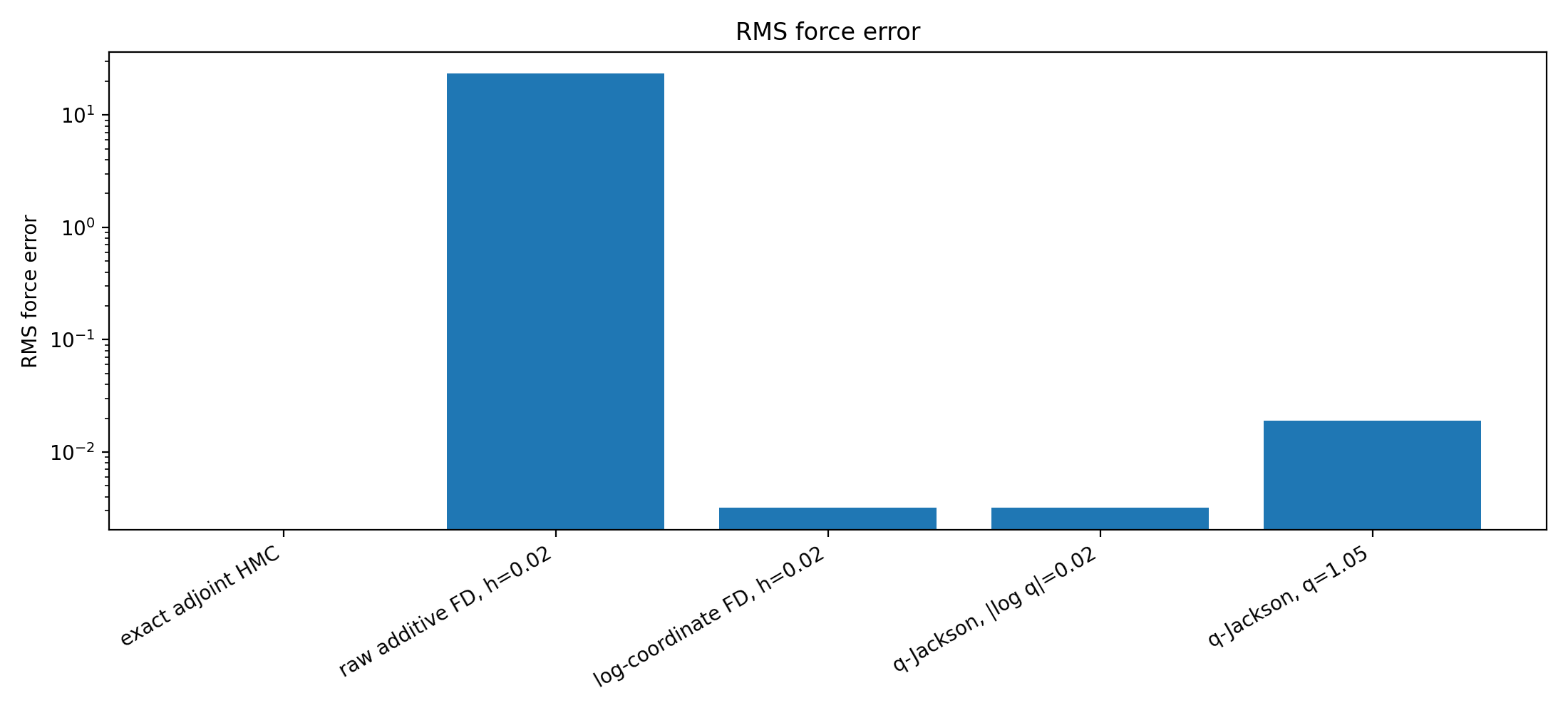
Table 5 reports the numerical results. The exact adjoint HMC provides the reference force. The raw additive finite-difference force has a substantially larger force error than all multiplicative or log-coordinate approximations. Its RMS force error is $2.34\times 10^{1}$ , whereas the log-coordinate finite difference and the symmetric $q$ -Jackson force with $|\log q|=0.02$ both have force error $3.18\times 10^{-3}$ . This confirms that, for a positive coefficient parameter, the multiplicative $q$ -Jackson perturbation reproduces the log-coordinate sensitivity much more accurately than a raw additive perturbation in the original coefficient variable.

The same effect is reflected in the Hamiltonian error. The median positive Hamiltonian error of the raw additive finite-difference method is $8.78\times 10^{0}$ , while the corresponding value for the $q$ -Jackson force with $|\log q|=0.02$ is $1.07\times 10^{-3}$ , essentially at the same scale as the exact adjoint and log-coordinate finite-difference benchmarks. The large energy error of the raw additive method also leads to a much lower acceptance rate, $0.159$ , whereas the adjoint, log-coordinate, and $q$ -Jackson variants all maintain acceptance rates close to one under the same integration parameters.

The reconstruction errors are of comparable magnitude across the stable methods. In this test, the log-coordinate finite difference gives the smallest relative coefficient error, while the two $q$ -Jackson variants remain close to the adjoint benchmark. Therefore, the main conclusion is not that $q$ -Jackson improves the coefficient reconstruction relative to adjoint HMC. Rather, the experiment shows that the $q$ -Jackson force is a scale-consistent black-box approximation to the adjoint force for positive functional parameters, while raw additive finite differences can introduce a severe scale mismatch.

This example should not be interpreted as replacing the adjoint method when an adjoint solver is available. Instead, it shows that the $q$ -Jackson multiplicative perturbation is consistent with adjoint sensitivity for positive functional parameters and can therefore be used as a scale-compatible black-box force approximation when only repeated evaluations of the coefficient-to-misfit map are available.

5 Conclusions

This paper developed a $q$ -deformed Hamiltonian Monte Carlo framework motivated by $q$ -deformed phase-space mechanics. Starting from a Lagrangian formulation, we derived the $q$ -Hamiltonian equations and proved the formal invariance of the associated $q$ -symplectic form within the $q$ -deformed differential calculus. These results provide the geometric basis for the proposed dynamics. For practical sampling, the formal $q$ -differential operators were realized through Jackson-type differences. This leads to a computable Metropolis-adjusted $q$ -Hamiltonian proposal. The Metropolis correction, not exact preservation of the formal $q$ -geometric structure after numerical realization, guarantees the validity of the Markov transition. We established detailed balance and recorded sufficient nondegeneracy conditions for irreducibility of the marginal position chain.

The numerical experiments clarify the computational role of the method. The $q$ -Jackson force provides a relative perturbation mechanism in the original coordinates. For positive variables, it corresponds to a centered finite difference in logarithmic coordinates; for mixed positive/signed targets, it can be applied directly without requiring a global logarithmic reparametrization. Across the tested examples, raw additive finite differences can suffer from domain violations, scale mismatch, large force errors, and large Hamiltonian errors. The $q$ -Jackson force avoids these failures and tracks exact-gradient, adjoint-force, log-coordinate, or scaled finite-difference benchmarks when such references are available.

The proposed method is not intended as a universal replacement for exact-gradient HMC, adjoint-based HMC, or modern adaptive HMC variants. Its main contribution is to connect $q$ -deformed Hamiltonian mechanics with a valid Metropolis-corrected sampling scheme and to show that the induced Jackson-type force can be useful for black-box or scale-sensitive targets. Future work should study adaptive selection of the deformation parameter, integration with standard HMC diagnostics, and applications to larger Bayesian models with constrained, multiscale, or mixed-coordinate parameters.

Hamiltonian Monte Carlo from qq-deformed phase-space mechanics

Abstract

keywords:

1 Introduction

2 A qq-Analogue of Hamiltonian Dynamics

2.1 qq-calculus and qq-Hamiltonian equations

2.2 Formal invariance of the qq-symplectic form

Theorem 1.

Proof.

Remark 1.

2.3 A computable realization through Jackson derivatives

Remark 2.

3 A Metropolis-adjusted qq-Hamiltonian sampler

3.1 The qq-Hamiltonian proposal

3.2 Detailed balance and invariance

Lemma 2.

Proof.

Theorem 3.

Proof.

Remark 3.

3.3 Irreducibility

Assumption 1.

Theorem 4.

Proof.

Remark 4.

Remark 5.

Remark 6.

4 Numerical tests

4.1 General setting, competing methods, and diagnostics

4.2 One-dimensional positive-scale black-box targets

4.3 High-dimensional synthetic positive-scale tests

4.4 Variance-component positive-scale black-box targets

4.5 A mixed log-trap target

4.6 Positive-coefficient diffusion inverse problem

5 Conclusions

References

Hamiltonian Monte Carlo from $q$ -deformed phase-space mechanics

2 A $q$ -Analogue of Hamiltonian Dynamics

2.1 $q$ -calculus and $q$ -Hamiltonian equations

2.2 Formal invariance of the $q$ -symplectic form

3 A Metropolis-adjusted $q$ -Hamiltonian sampler

3.1 The $q$ -Hamiltonian proposal