Spatially Varying Gene Regulatory Networks via Bayesian Nonparametric Covariate-Dependent Directed Cyclic Graphical Models
Abstract
Spatial transcriptomics technologies enable the measurement of gene expression with spatial context, providing opportunities to understand how gene regulatory networks vary across tissue regions. However, existing graphical models focus primarily on undirected graphs or directed acyclic graphs, limiting their ability to capture feedback loops that are prevalent in gene regulation. Moreover, ensuring the so-called stability condition of cyclic graphs, while allowing graph structures to vary continuously with spatial covariates, presents significant statistical and computational challenges. We propose BNP-DCGx, a Bayesian nonparametric approach for learning spatially varying gene regulatory networks via covariate-dependent directed cyclic graphical models. Our method introduces a covariate-dependent random partition as an intermediary layer in a hierarchical model, which discretizes the covariate space into clusters with cluster-specific stable directed cyclic graphs. Through partition averaging, we obtain smoothly varying graph structures over space while maintaining theoretical guarantees of stability. We develop an efficient parallel tempered Markov chain Monte Carlo algorithm for posterior inference and demonstrate through simulations that our method accurately recovers both piecewise constant and continuously varying graph structures. Application to spatial transcriptomics data from human dorsolateral prefrontal cortex reveals spatially varying regulatory networks with feedback loops, identifies potential cell subtypes within established cell types based on distinct regulatory mechanisms, and provides new insights into spatial organization of gene regulation in brain tissue.
Keywords: Directed cyclic graphs; Covariate dependent partition model; Parallel tempering; MCMC; Covariate-dependent graphs
1 Introduction
Single-cell RNA sequencing (scRNA-seq) has revolutionized our understanding of cellular heterogeneity and gene expression by enabling the characterization of distinct cell types within complex tissues. Despite its widespread applications in fields such as cancer research, immunology, and neuroscience, scRNA-seq alone lacks spatial context, which is crucial for addressing many biological questions. Spatial transcriptomics bridges this gap by integrating scRNA-seq with spatial localization within tissues. This spatial information provides critical insights into gene expression patterns and spatially regulated functions. For instance, brain function is closely tied to the spatial organization of neuronal and glial cells. Spatial transcriptomics techniques can be broadly classified into four categories: (i) sequencing-based (e.g., 10x Genomics Visium, Slide-seq, Stereo-seq, Light-seq); (ii) probe-based (e.g., GeoMx); (iii) imaging-based (e.g., CosMx SMI, MERFISH, seqFISH, seqFISH+); and (iv) image-guided spatially resolved scRNA-seq (e.g., Geo-seq, Zipseq). For an overview of spatial transcriptomics technologies, we refer to Chen et al. (2023b).
Building on advancements in spatial transcriptomics, a critical step in analyzing such data is to understand spatially varying gene regulatory networks (svGRNs), which capture how gene regulatory interactions change across tissue regions. Unlike traditional gene regulatory networks (GRNs), which assume uniform regulatory interactions, svGRNs account for spatial heterogeneity by incorporating cellular location and local microenvironmental influences. The existence of spatially varying genes, whose expression levels change across different spatial regions, and the existence of cellular heterogeneity are indications of svGRNs, as these variations in expression and cellular functions often arise from localized regulatory interactions (Wang et al., 2022a). Various computational approaches have been developed to identify spatially varying genes, including model-based methods (e.g., SpatialDE (Svensson et al., 2018), SPARK (Sun et al., 2020), SPARK-X (Zhu et al., 2021)), neighborhood-based methods (e.g., Giotto (Dries et al., 2021), nnSVG (Weber et al., 2023), MERINGUE (Miller et al., 2021)), and statistical measures such as Moran’s I (Moran, 1950), as implemented in the Seurat package (Hao et al., 2023, 2021; Stuart et al., 2019; Butler et al., 2018; Satija et al., 2015). While identifying spatially varying genes has been extensively studied, uncovering svGRNs is underexplored and could provide deeper insights into spatially regulated biological processes, developmental patterns, and disease mechanisms.
Our motivating application involves analyzing spatial transcriptomics data from the human dorsolateral prefrontal cortex (Maynard et al., 2021), where cells exhibit distinct spatial organization across tissue layers. For instance, Figure 1.1 displays the spatial distribution of gene expression levels for eight selected genes from neurons, revealing clear spatial patterns and heterogeneity. Traditional GRN analyses assume uniform regulatory relationships across all cells of a given type. However, the spatial organization of brain tissue suggests that gene regulatory interactions may vary across different tissue regions, even within the same cell type. Our goal is to infer svGRNs that capture how regulatory relationships change with cellular location, potentially revealing distinct regulatory mechanisms in different microenvironments. Such analysis requires methods capable of learning directed cyclic graphs to capture feedback loops inherent in gene regulation while accounting for spatial heterogeneity.

The construction of GRNs from gene expression data while incorporating spatial cell location information aligns closely with broader statistical research on graph learning from heterogeneous data. This area has gained significant attention due to its applications in various biological domains, such as cancer genomics, where molecular and genomic heterogeneity is prevalent (Heppner and Miller, 1983). Much of the existing work in this field focuses on leveraging auxiliary information to recover graph structures and has been dedicated to learning either covariate-assisted undirected graphs (UGs) or directed acyclic graphs (DAGs), limiting their ability to capture feedback loops and spatial variations in gene regulation.
Research on UG learning is extensive, with various studies exploring covariate-dependent Gaussian graphical models (GGMs) to infer graph structures while adjusting for covariates on the mean level (Yin and Li, 2011; Li et al., 2012; Cai et al., 2013; Bhadra and Mallick, 2013; Lin et al., 2016; Chen et al., 2016; Ni et al., 2018a; Deshpande et al., 2019; Niu et al., 2020). Some approaches have considered modeling covariate-dependent precision matrices (Zhou et al., 2010; Fox and Dunson, 2015; Lee and Xue, 2018; Xie et al., 2020; Zeng et al., 2024). While these methods improve UG structure learning in heterogeneous data, they often assume a single homogeneous UG structure across populations. To address this limitation, researchers have developed approaches for learning multiple graphs in grouped settings (Guo et al., 2011; Danaher et al., 2014; Peterson et al., 2015; Mitra et al., 2016; Xie et al., 2016; Tan et al., 2017; Lin et al., 2017; Shaddox et al., 2018) and mixtures of GGMs to estimate cluster-specific graphs (Rodriguez et al., 2011; Talluri et al., 2014). Other works have introduced regression-based or partition-based methods to allow graph structure to vary with covariates (Liu et al., 2010; Ni et al., 2022; Wang et al., 2022b; Niu et al., 2023; Zhang and Li, 2023; Chen et al., 2023a; Yao et al., 2025). In the bioinformatics literature, there are some attempts to infer gene co-expression networks from spatial transcriptomic data (Li et al., 2025; Fang et al., 2023; DeTomaso and Yosef, 2021; Wei et al., 2022; Acharyya et al., 2022), but they too mostly rely on UGs.
DAG learning has also been widely explored, with efforts to account for population heterogeneity in grouped settings (Oates et al., 2014; Yajima et al., 2015). More recent work has developed methods for continuously varying DAG structures (Ni et al., 2019; Zhou et al., 2023b) and covariate-dependent quantile DAG estimation (Sagar et al., 2022). However, despite the great advancements, these approaches either impose strict acyclicity constraints or fail to capture the inherent asymmetry in gene regulation, limiting their applicability in constructing GRNs with possible feedback loops.
To address these challenges, some studies have explored learning directed cyclic graphs (DCGs), which accommodate feedback loops. Notable approaches include the cyclic causal discovery (CCD) algorithm (Richardson, 1996), the independent component analysis-based LiNG-D algorithm (Lacerda et al., 2012), and the cyclic additive noise models (Mooij et al., 2011). However, these methods were not designed to accommodate covariates or model non-iid/heterogeneous data. Ni et al. (2018a, b) incorporated covariates but only on the mean level, and hence the graph remains the same for all observations. Unlike UG and DAG learning, one unique challenge of inferring DCGs whose structures vary with covariates is that the stability condition, which is an eigenvalue condition on the causal effect matrix (detailed in Section 2), has to be satisfied at any given covariate value or spatial location.
In this article, we introduce a novel method, called Bayesian nonparametric directed cyclic graph with covariates (BNP-DCGx), to infer directed cyclic svGRNs from spatial transcriptomic data. To accommodate distinct graph structures influenced by spatial variation, we introduce a covariate-dependent random partition layer within a Bayesian hierarchical model, serving as an intermediary between covariates and DCGs. This hierarchical learning framework learns finite partition-dependent DCGs that satisfy the stability condition and then refines them through partition averaging, effectively capturing gene regulatory interactions continuously varying over space. This is, to our knowledge, the first approach that allows for the modeling of svGRNs with feedback loops while accounting for spatial heterogeneity.
The rest of the article is organized as follows. Section 2 introduces the notations, general formulation, and the proposed model, detailing the likelihood, prior distributions, and random partition-based cyclic graphical models. Section 3 discusses posterior inference using a parallel tempered Markov chain Monte Carlo (MCMC) sampler, practical implementation of partition averaging, and the theoretical guarantee of satisfying the stability condition for partition-specific DCGs. Section 4 establishes theoretical support for the proposed method. Section 5 provides simulations, including cluster-specific graphs and continuously varying covariate-dependent DCGs. Finally, Section 6 applies the proposed method to the motivating spatial transcriptomics data to infer svGRNs, followed by a discussion in Section 7.
2 Proposed Model
2.1 Notations, Backgrounds, and General Formulation
Let denote a vector of gene expressions for cell . Let denote a vector of covariates, which are 2-dimensional spatial locations in our application (hence ). For any positive integer , let and let be a shorthand for .
Traditionally, constructing GRNs ignores ’s and is only based on ’s, which are assumed to be iid. Specifically, a structural equation model (Bollen, 1989, SEM) is often used,
| (2.1) |
where is a vector of intercepts, is a matrix of SEM coefficients representing gene regulatory effects in our application, and is a vector of jointly independent noises. To connect SEM with a graph, we draw an arrow meaning gene regulates gene if . It can be shown that the SEM in (2.1) is globally Markov with respect to the resulting graph, i.e., it respects all the conditional independence relationships encoded in the graph via the notion of d-separation (Spirtes, 1995). If the graph is constrained to be acyclic, the SEM is a Bayesian network model (Peal, 1985). However, generally, the graph need not be acyclic. For instance, if and , then . For historic reasons, directed graphs without acyclic constraints are called DCGs even though they are not required to contain directed cycles. The diagonal entries of are often fixed to 0 to avoid self-loops. DCGs and SEMs have been widely used in engineering (Mason, 1953) and econometrics (Haavelmo, 1943) to represent dynamic processes in equilibrium with the assumption of stability (Fisher, 1970). An SEM is stable if the modulus of the eigenvalues of is less than or equal to 1, and no eigenvalue is 1. Under the stability condition, the SEM and its associated DCG can be viewed as a compact representation of an infinite DAG of variables indexed by time (Spirtes, 1995).
In this paper, we will relax the iid assumption and allow the graph to vary with covariates (spatial locations) by extending (2.1) to
| (2.2) |
where and map covariates to the SEM intercepts and coefficients. Because encodes the graph structure, the graph can vary with covariates in our model. The main challenge is how to model the mapping so that satisfies the stability condition for any .
Definition 1 (Stable Function).
We say a matrix-variate function is stable if is stable for any
Natural modeling choices such as splines and Gaussian processes would find it quite hard to ensure the stability of . For instance, one might attempt to expand for some basis functions . Then it seems unattainable to introduce and implement a set of constraints on or to force all the eigenvalues of for any to have modulus less than or equal to 1.
To overcome this challenge, we propose a novel Bayesian nonparametric covariate-dependent DCG model, BNP-DCGx, which is illustrated in Figure 2.1. The main idea is to not contemplate explicit expression of but instead introduce an intermediary between and in a Bayesian hierarchical formulation, which is designed to enable a simple strategy for imposing the stability constraints while maintaining functional flexibility. We choose the intermediary to be a covariate-dependent infinite partition, which has some desirable properties. First, conditional on the partition, is discretized into , each of which complies with the stability condition straightforwardly. Second, marginalizing out the partition, we recover , which is guaranteed to be stable for any . Hence, our model can be viewed from two different perspectives, namely, the cluster view and the functional view. Third, the partition size (i.e., the number of clusters) grows with sample size, which gives rise to a flexible representation of . The general hierarchical formulation is as follows (for simplicity, some parameters such as the intercepts are omitted),
| (2.3) |
where is a partition of . We call a cluster, and the number of clusters is allowed to grow with . A key feature of this formulation is that is no longer explicitly expressed as in (2.2). It is replaced by countably many ’s for which the prior distributions, to be specified later, can easily accommodate the stability constraint. Because ’s are only defined conditionally on the clusters/partition, we call (2.3) the cluster view of the proposed model.
Although is not explicit in (2.3), it is implicitly defined as
where is the cluster indicator of unit with if for . Marginalizing out , we arrive at the functional view of the proposed model – a mixture distribution of ,
where is the collection of all partitions of and is the indicator function. We will show that
Denote to be the set of all stable matrices. Then the following holds,
The second equality holds because conditional on a random partition , the cluster indicators are non-random quantities and . Moreover, each of the satisfy the stability condition.
For the rest of this section, we will specify the sampling distribution, priors on that respects the stability condition, the covariate-dependent partition prior, and priors of other parameters omitted in (2.3).

2.2 Sampling Distribution
To specify the sampling distribution of ’s is to specify the distribution of the noises ’s. Although Gaussian would be a tempting choice, it should be avoided for identifiability. Gaussian noises would render the same sampling distribution for Markov equivalent DCGs (i.e., DCGs that encode the same set of conditional independence relationships), and hence those DCGs cannot be distinguished from each other even with an infinite sample size. Fortunately, Gaussian noises are a peculiar case in that any non-Gaussian noises would resolve the identifiability issue thanks to the identifiability theory of independent component analysis (Lacerda et al., 2012). Therefore, in this paper, we choose noises to be Laplace-distributed,
for and . For ease of computation, we equivalently represent the Laplace distribution as a scale mixture of normal,
Then via the change of variables, the sampling distribution of ’s is given by,
where is a -dimensional identity matrix and is matrix determinant.
2.3 Covariate-Dependent Partition Prior
The partition is the crucial intermediary between and , which ultimately leads to a stable . We consider the product partition model with covariates (Müller et al., 2011, PPMx),
| (2.4) |
where , is a similarity function characterizing the similarity among , and is the cohesion function capturing the tightness of . For ease of computation, we follow the recipe in Müller et al. (2011) by setting,
| (2.5) | ||||
| (2.6) |
where is the size of cluster . These specifications of the similarity and the cohesion functions would later allow us to reformulate our full model with augmented parameters as a Dirichlet process mixture model for which many existing posterior sampling algorithms can be employed.
The auxiliary probability models and in (2.5) are given by,
| (2.7) |
where is the inverse-Wishart distribution with degrees of freedom and an identity scale matrix .
2.4 Stable Spike-and-Slab and Cascade Priors
Conditional on the partition, we assign priors to the cluster-specific parameters . The SEM coefficient matrix needs to be both sparse and stable. To achieve this, we propose a stable spike-and-slab (SSS) prior,
| (2.8) | ||||
where is the collection of all stable matrices, , is a very small fixed constant, is a -dimensional vector created by stacking the columns of without the diagonal entries, , , , and is a normalizing factor,
The binary indicator indicates whether is present in cluster because the spike is very tightly concentrated on 0 whereas the slab is dispersed.
Because the SSS prior enforces stability via , the normalizing factor is intractable. To avoid evaluating it in the calculation of the full conditional distributions of , we assume the following joint prior on ,
| (2.9) |
where is the inverse-gamma distribution and the normalizing factor is given by,
Including in serves to cancel out its reciprocal in when deriving the full conditional distributions for and . With this specification, their full conditionals are Bernoulli and inverse-gamma. In the same vein, we include in the prior of to have closed-form full conditional,
| (2.10) |
where
Although none of the normalizing factors , is analytically available, they are all finite (e.g., is bounded by 1 because it is an integral of a probability density function over a subspace) and never have to be evaluated in our posterior inference algorithm. Because cascades through via , we call the joint prior (2.8)-(2.10) as the cascade prior.
We complete our model with conjugate priors on the intercepts and the noise scale parameters,
2.5 Partition Averaging
As mentioned in Section 2.1, the proposed BNP-DCGx has dual views. Conditional on the partition, the model identifies cluster-specific DCGs, whereas with the partition marginalized out, the functional view is manifested,
Although complicated in form, is a discrete mixture of truncated, degenerated multivariate Gaussians with mixture weights . The truncation is due to the stability constraint , and the degeneracy reflects the piecewise constant nature of the representation of via partition.
For an unseen observation , the posterior predictive distribution of is given by
| (2.11) | ||||
where , which is a partition of obtained by adding unit to cluster in . We show that the stability condition is preserved with probability one.
Proposition 1.
Under the proposed model, .
Proof.
The second equality is because conditional on , for any . The third equality is because the SSS prior proposed in Section 2.4 ensures for any . ∎
3 Posterior Inference
3.1 Markov Chain Monte Carlo
The proposed model is parameterized by for , , and . All but and is sampled via closed-form Gibbs. Metropolis-within-Gibbs is used for sampling and . All sampling steps are provided below.
-
•
Sample .
-
•
Sample where .
-
•
Sample where .
-
•
Sample where .
-
•
Sample where .
-
•
Sample by random-walk Metroloplis-within-Gibbs. We propose . If the resulting is not stable, reject it; otherwise, accept it with probability
(3.1) where , , and is the marginal likelihood with ’s integrated out,
(3.2) -
•
Sample where is the generalized inverse Gaussian distribution with density proportional to .
-
•
Sample from a categorical distribution with probability
(3.3) where , and and are the observations in the cluster except for the one. For better mixing, we have marginalized out in (3.3). The prior conditional distribution of is the well-known Chinese restaurant process,
(3.4) where with . The conditional distribution of is given by,
(3.5) with
where , and and are drawn from their respective prior distributions. The conditional distributions for is multivariate t distribution,
(3.6) with
For better mixing, we employ the parallel tempering technique (Swendsen and Wang, 1986; Geyer, 1991) by running Markov chains in parallel with different but related target distributions. The target distribution is proportional to the fractional power of the likelihood multiplied by the prior. In particular for a sequence of increasing “temperature” values , we have the target distribution as the following,
| (3.7) | ||||
for any . Choosing an increasing sequence of “temperature” values ensures we have our desired posterior distribution for along with a set of heated chains. This helps the algorithm explore the parameter space more efficiently by using a flattened likelihood, which is less susceptible to being trapped in local modes.
In addition to the update of parameters within each chain (as described in Section 3.1), once every certain number of iterations, we propose to swap the states of two chains (say and ) and accept it according to a Metropolis-Hastings (MH) ratio,
| (3.8) |
where the superscript indexes the chain (e.g., is the cluster-specific indicators for the observation obtained from the chain ).
3.2 Implementation of Partition Averaging with Stability Guarantee
The partition averaging described in Section 2.5 can be carried out straightforwardly with MCMC samples. For instance, for an unseen observation , the posterior mean of can be computed as follows:
where indexes the MCMC sample and can be drawn from the following conditional distribution,
for which the closed-form expressions are similar to (3.4) and (3.6).
4 Large prior support
Recall that our prior model entails , i.e., is a piecewise constant function. Despite the discrete nature, we show that our prior places positive mass around any Hlder continuous and , or in other words, the proposed model is flexible enough for modeling continuously varying DCG.
Theorem 2.
Suppose be any matrix of SEM coefficients and be the intercept vector as in Equation (2.1), where , are continuous functions for univariate with . We assume that all the entries of and belong to the space of uniformly Hlder continuous functions. Then for any , there exists such that
-
(i)
For any absolutely continuous prior distributions on and on
we have,where be the set of stable matrices and for .
-
(ii)
Similarly, for any absolutely continuous prior distributions on and on we have,
where is of the same form as part of the theorem.
5 Simulation study
We assess the performance of the proposed BNP-DCGx under two different simulation scenarios. The first simulation demonstrates the capability of BNP-DCGx in learning the cluster-specific graph structures (i.e., the cluster view). The other simulation examines the partition averaging for DCGs that vary with covariates (i.e., the functional view) using continuous function. Throughout the simulations and the real data analysis, we use the same set of hyperparameters: . We run four parallel chains with temperature values and swap the chains every iterations.
5.1 Cluster-Specific Graphs
In this scenario, we consider cluster-specific covariate-dependent DCGs with nodes. The true DCGs are provided in Figure 5.1 (shown as the red edges) with the edge coefficients generated from where . In each cluster, we have observations, leading to a total of observations for this experiment. The three cluster-specific intercepts and are generated from , , and , respectively. The errors are generated from where for with . We then let . Finally, the covariates , for , are sampled from , , and , respectively.

We generate MCMC samples from the proposed BNP-DCGx with burn-in of samples. We report the estimated cluster-specific DCGs in Figure 5.1, shown as blue edges. We compare our method with two alternative methods: (i) the cyclic causal discovery (CCD) algorithm (Richardson, 1996) and (ii) a special case of the proposed method without covariates and clusters (called DCG hereafter). Both methods allow for the modeling of directed cycles but assume that the graph is the same across clusters. In Table 5.1, we report true positive rate (TPR), false discovery rate (FDR), and Matthew’s correlation coefficient (MCC) for all methods calculated over 20 replicates:
where TP = number of true positives, FP = number of false positives, TN = number of true negatives, and FN = number of false negatives. It clearly demonstrates the capability of our method in learning cluster-specific DCGs with high TPR and MCC, as well as a low FDR. The competing methods have high FDR, highlighting the importance of accounting for heterogeneity in graph learning when heterogeneity is present.
| Methods | Measures | Cluster | Cluster | Cluster |
|---|---|---|---|---|
| BNP-DCGx | TPR | |||
| FDR | ||||
| MCC | ||||
| DCG | TPR | |||
| FDR | ||||
| MCC | ||||
| CCD | TPR | |||
| FDR | ||||
| MCC |
5.2 Continuous Graph Functions
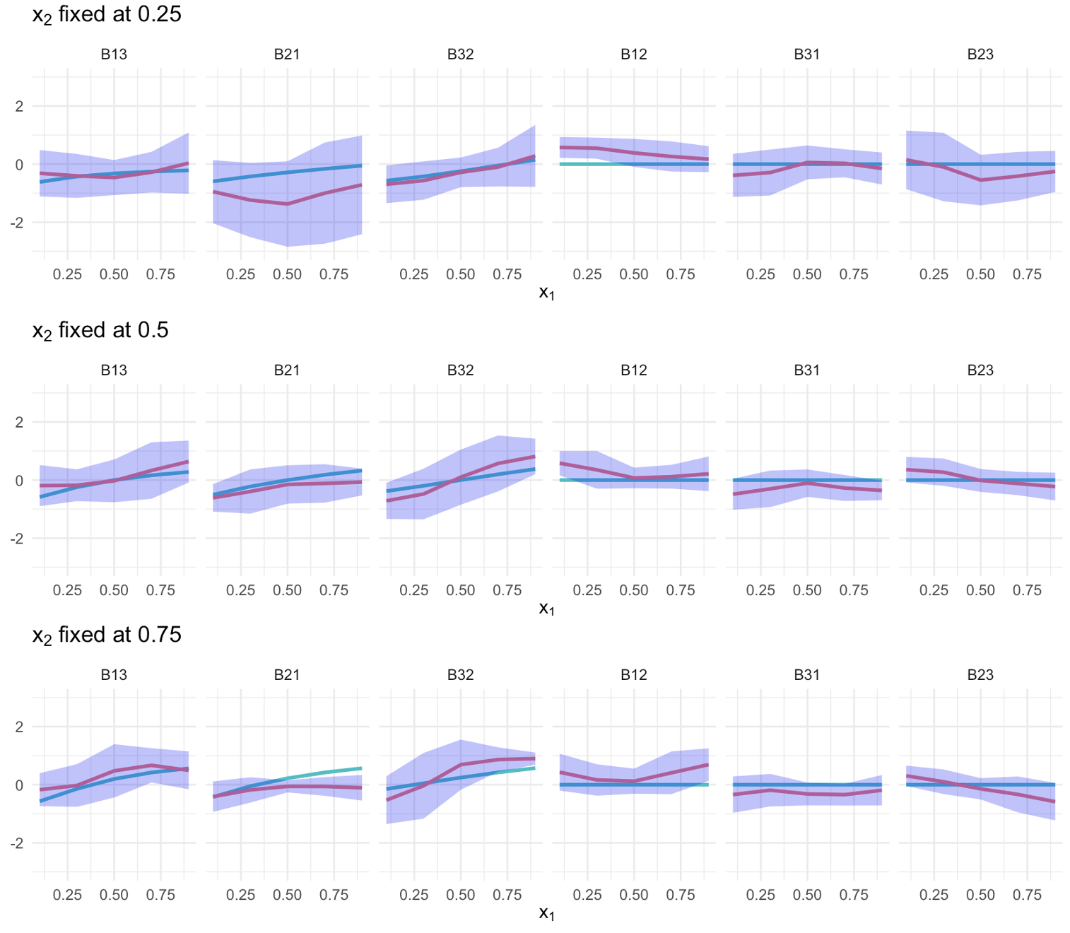
In this scenario, we consider a fixed graph (i.e., one cluster) with continuously varying . For ease of demonstration, we consider and . The sample size is set to . The true graph is a cycle . The nonzero entries of the true is a function of covariates specified as follows:
where , and . The rest of the entries of the matrix is zero. We set . We generate the noise terms from normal, , with and drawn from for . Subsequently, we set . We uniformly sample the covariates . Like before, we generate MCMC samples with burn-in of samples.

6 Real Data Analysis
We analyzed the motivating spatial transcriptomics data collected from the six-layered human dorsolateral prefrontal cortex (Maynard et al., 2021) to infer svGRNs. The metadata indicate seven different broad cell types. We arranged our analysis into four tissue segments: excitatory neurons (n=1774), other neurons (n=650), oligodendrocytes and oligodendrocyte-like cells (oligodendrocytes hereafter for short, n=991), and astrocytes (n=1180). Excitatory neurons and other neurons exhibit double-band structures (see the left panels of Figures 6.2 and 6.3), oligodendrocytes consist of several similar cell subtypes that are spatially adjacent (Figure 6.4, left panel), and astrocytes form a single band structure (Figure 6.5, left panel). For objectivity, we selected eight genes with the highest correlations, which is necessary for graph learning, for each tissue segment. These selected genes turn out to be biologically relevant as they are significantly enriched for brain functions (Figure 6.1). We generated posterior samples with burn-in from the proposed BNP-DCGx using the parallel tempered MCMC.


We depict the union of all the spot-level svGRNs as a cell-population-level summary for the excitatory neurons, other neurons, oligodendrocytes, and astrocytes in the right panels of Figures 6.2, 6.3, 6.4, and 6.5, respectively. The edge width reflects the frequency of occurrence of the edges across all spot-level individual svGRNs. Highly connected hub genes across spot-level svGRNs tend to play crucial roles in gene regulation as they are involved in many regulatory activities for many cells. In the excitatory neurons, SST, a neuropeptide, plays a central role mostly in brain functions and cognitive behavior. A reduction in the expression of SST could be an important indication of neurological disorders such as depression and Alzheimer’s disease (Song et al., 2021). Alfimova et al. (2021) suggests that the methylated YJEFN3 is involved with cognitive deficits such as schizophrenia spectrum disorders. CXCL14 contributes towards a wide variety of biological processes such as neural development and immune process (Westrich et al., 2020; Zhou et al., 2023a). In other neurons, BEX5 is a hub and is one of the members of the family of BEX proteins in humans, which is involved in signaling pathways and transcriptional regulations for neurodegenration and cell growth (Fernandez et al., 2015). HMGB1 is responsible for a wide variety of mechanisms mostly related to aging and age-related diseases, inflammatory diseases, and immunity (Martinotti et al., 2015; Yuan et al., 2020; Guan et al., 2023; Ruggieri et al., 2024). In Oligodendrocytes, GFAP is a biomarker for neurological disorders and could cause Alexander disease through mutation (Quinlan et al., 2007; Yang and Wang, 2015).
We select some spots, whose spatial locations are highlighted in the left panels of Figures 6.2-6.5, for the visualization of spot-level svGRNs in Figures 6.6-6.11. The edge width represents the posterior inclusion probability of the edge. Many of them contain at least one feedback loop, which cannot be detected with existing DAG learning algorithms. For the neurons (Figures 6.6-6.9), we notice an interesting similarity in the structure of svGRNs within each band-like structure and the difference between the two bands. For example, the two svGRNs displayed in Figure 6.8, one from each band, reveal notable differences in both edge inclusion and edge strengths. Conversely, the svGRNs corresponding to spots within the same band, e.g., the pair in Figure 9(a) and the pair in Figure 9(b) exhibit structural similarity with small variations in edge strengths. The larger dissimilarity between the bands indicates regulatory heterogeneity for cells of the same type, which may be due to microenvironmental factors.


Such spatial regulatory heterogeneity cannot be captured by conventional spatial transcriptomic clustering algorithms. For example, we applied the Dimension-Reduction Spatial-Clustering (DR-SC) (Liu et al., 2022) designed for spatial transcriptomics data as well as the traditional k-means algorithm with . The left panel of Figure 6.12 presents the k-means clustering based solely on gene expression data, while the middle panel shows the clustering obtained using a combined and scaled version of both gene expression and spatial information. Clearly, k-means failed to detect the two bands as two separate clusters. In the former case, the two clusters are mixed within each band with no clear separation. In the latter case, while some localization of the two clusters is observed, the clusters do not correspond to the two spatial bands. Instead, each band contains roughly two clusters with some interspersed points in the middle of the bands. The right panel of Figure 6.12 shows that only one cluster was found by DR-SC. Failure to detect the distinct two bands could be explained by the unimodal marginal distributions of the gene expression (results not shown). The proposed method could successfully detect the two spatial bands, which could be novel neuron subtypes, by leveraging the underlying differences in their GRNs in addition to the gene expression differences.

The identification of cell subtypes is biologically plausible. As stated by Maynard et al. (2021), the human dorsolateral prefrontal cortex can be characterized by its laminar organization, that is, by the arrangement of cortical neurons into six distinct layers. The cell type and spots within different cortical layers can exhibit distinct gene expression profiles and varying connectivity patterns of genes. Moreover, advancements in single-cell transcriptomics and the continuous refinement of cell type classifications have uncovered the existence of remarkable diversity in cortical cell subtypes. Refer to Miller et al. (2019) for details on cellular diversity and subtypes in the human cerebral cortex. This diversity arises during development where specialized groups of immature cells, known as progenitor pools, give rise to a variety of cell types and subtypes. Consequently, within a single cell type, there may exist distinct cellular microenvironments or multiple cell subtypes, potentially leading to differences in gene regulatory relationships.
In summary, the proposed method detected svGRNs with feedback loops based on spatial transcriptomic data using spatial locations as covariates. Moreover, the inferred graph structures reveal distinct clusters corresponding to separated spatial bands, allowing the identification of plausible cell subtypes driven by distinct GRNs. While GRNs within the same band may exhibit structural similarities, the variation in edge strength highlights their spatial dynamics. This suggests the potential influence of the cellular microenvironment on GRNs, emphasizing the role of spatially varying connectivity within the tissue context.
7 Discussion
We have proposed a novel Bayesian nonparametric directed cyclic graph model, BNP-DCGx, which leverages covariate information in heterogeneous data through a covariate-dependent random partition model. The key feature is the use of an intermediary partition layer between covariates and graph structures, which enables us to satisfy the stability condition, an eigenvalue constraint on the SEM coefficient matrix, while allowing graph structures and edge strengths to vary continuously with covariates. We developed a parallel-tempered MCMC algorithm and ensured smoothly varying graphs through partition averaging from a set of discrete graphs originated from the random partition. The efficacy of the proposed method was demonstrated through simulations and an application to spatial transcriptomics data from human dorsolateral prefrontal cortex. In the real data analysis, the method identified graph structures with feedback loops that vary across spatial locations within a single cell type. Notably, the inferred regulatory networks revealed distinct clusters corresponding to separated spatial bands, identifying plausible cell subtypes driven by distinct gene regulatory mechanisms. These regulatory subtypes were not detected by conventional clustering methods based on gene expression alone, highlighting the value of network-level analysis for uncovering hidden heterogeneity. The variation in edge strengths within spatial bands further suggests the influence of local microenvironmental factors on gene regulation, emphasizing the role of spatially varying connectivity within tissue context.
Future research directions include extending the model to accommodate confounders, exploring non-linear relationships beyond the current linear structural equation framework, and investigating alternative approaches for constructing covariate-dependent cyclic graphs. The computational efficiency could be improved through variational Bayes approximations for large graphs or datasets. The identification of regulatory subtypes based on network differences opens new avenues for precision medicine, where treatments could be tailored to an individual’s regulatory profile rather than expression profile alone. As spatial multi-omics technologies continue to advance, methods that integrate spatial information with regulatory network inference will become increasingly valuable for understanding the complex organization of biological systems. Beyond spatial transcriptomics, the proposed framework has broad applicability in diverse fields where feedback mechanisms and heterogeneity are expected, such as dynamic brain networks in neuroscience, metabolic and signaling pathways in systems biology, and simultaneous equation models in econometrics.
References
- SpaceX: gene co-expression network estimation for spatial transcriptomics. Bioinformatics 38 (22), pp. 5033–5041. Cited by: §1.
- Relationship between dna methylation within the yjefn3 gene and cognitive deficit in schizophrenia spectrum disorders. Russian Journal of Genetics 57 (9), pp. 1092–1099. Cited by: §6.
- Joint high-dimensional bayesian variable and covariance selection with an application to eqtl analysis. Biometrics 69 (2), pp. 447–457. Cited by: §1.
- Structural equations with latent variables.. Cited by: §2.1.
- Integrating single-cell transcriptomic data across different conditions, technologies, and species. Nature Biotechnology 36, pp. 411–420. External Links: Document, Link Cited by: §1.
- Covariate-adjusted precision matrix estimation with an application in genetical genomics. Biometrika 100 (1), pp. 139–156. Cited by: §1.
- Probabilistic graphical modeling under heterogeneity. bioRxiv, pp. 2023–10. Cited by: §1.
- Asymptotically normal and efficient estimation of covariate-adjusted gaussian graphical model. Journal of the American Statistical Association 111 (513), pp. 394–406. Cited by: §1.
- Spatial transcriptomic technologies. Cells 12 (16), pp. 2042. Cited by: §1.
- The joint graphical lasso for inverse covariance estimation across multiple classes. Journal of the Royal Statistical Society Series B: Statistical Methodology 76 (2), pp. 373–397. Cited by: §1.
- Simultaneous variable and covariance selection with the multivariate spike-and-slab lasso. Journal of Computational and Graphical Statistics 28 (4), pp. 921–931. Cited by: §1.
- Hotspot identifies informative gene modules across modalities of single-cell genomics. Cell systems 12 (5), pp. 446–456. Cited by: §1.
- Giotto: a toolbox for integrative analysis and visualization of spatial expression data. Genome biology 22, pp. 1–31. Cited by: §1.
- Subcellular spatially resolved gene neighborhood networks in single cells. Cell Reports Methods 3 (5). Cited by: §1.
- Brain expressed and x-linked (bex) proteins are intrinsically disordered proteins (idps) and form new signaling hubs. PloS one 10 (1), pp. e0117206. Cited by: §6.
- A correspondence principle for simultaneous equation models. Econometrica: Journal of the Econometric Society, pp. 73–92. Cited by: §2.1.
- Bayesian nonparametric covariance regression. The Journal of Machine Learning Research 16 (1), pp. 2501–2542. Cited by: §1.
- Markov chain Monte Carlo maximum likelihood. In Computing science and statistics: Proceedings of the 23rd Symposium on the Interface, Vol. 156163. Cited by: §3.1.
- The comprehensive role of high mobility group box 1 (hmgb1) protein in different tumors: a pan-cancer analysis. Journal of inflammation research, pp. 617–637. Cited by: §6.
- Joint estimation of multiple graphical models. Biometrika 98 (1), pp. 1–15. Cited by: §1.
- The statistical implications of a system of simultaneous equations. Econometrica, pp. 1–12. Cited by: §2.1.
- Integrated analysis of multimodal single-cell data. Cell. External Links: Document, Link Cited by: §1.
- Dictionary learning for integrative, multimodal and scalable single-cell analysis. Nature Biotechnology. External Links: Document, Link Cited by: §1.
- Tumor heterogeneity: biological implications and therapeutic consequences. Cancer and Metastasis Reviews 2, pp. 5–23. Cited by: §1.
- Enrichr: a comprehensive gene set enrichment analysis web server 2016 update. Nucleic acids research 44 (W1), pp. W90–W97. Cited by: Figure 6.1, Figure 6.1.
- Discovering cyclic causal models by independent components analysis. arXiv preprint arXiv:1206.3273. Cited by: §1, §2.2.
- Nonparametric finite mixture of gaussian graphical models. Technometrics 60 (4), pp. 511–521. Cited by: §1.
- Sparse estimation of conditional graphical models with application to gene networks. Journal of the American Statistical Association 107 (497), pp. 152–167. Cited by: §1.
- SpaGRN: investigating spatially informed regulatory paths for spatially resolved transcriptomics data. Cell Systems 16 (4). Cited by: §1.
- Penalized maximum likelihood estimation of multi-layered gaussian graphical models. Journal of Machine Learning Research 17 (146), pp. 1–51. External Links: Link Cited by: §1.
- On joint estimation of gaussian graphical models for spatial and temporal data. Biometrics 73 (3), pp. 769–779. Cited by: §1.
- Graph-valued regression. Advances in Neural Information Processing Systems 23. Cited by: §1.
- Joint dimension reduction and clustering analysis of single-cell rna-seq and spatial transcriptomics data. Nucleic acids research 50 (12), pp. e72–e72. Cited by: §6.
- Emerging roles for hmgb1 protein in immunity, inflammation, and cancer. ImmunoTargets and therapy, pp. 101–109. Cited by: §6.
- Feedback theory-some properties of signal flow graphs. Proceedings of the IRE 41 (9), pp. 1144–1156. Cited by: §2.1.
- Transcriptome-scale spatial gene expression in the human dorsolateral prefrontal cortex. Nature neuroscience 24 (3), pp. 425–436. Cited by: §1, §6, §6.
- Characterizing spatial gene expression heterogeneity in spatially resolved single-cell transcriptomic data with nonuniform cellular densities. Genome research 31 (10), pp. 1843–1855. Cited by: §1.
- Shared and derived features of cellular diversity in the human cerebral cortex. Current opinion in neurobiology 56, pp. 117–124. Cited by: §6.
- Bayesian graphical models for differential pathways. Cited by: §1.
- On causal discovery with cyclic additive noise models. Advances in Neural Information Processing Systems 24. Cited by: §1.
- Notes on continuous stochastic phenomena. Biometrika 37 (1/2), pp. 17–23. Cited by: §1.
- A product partition model with regression on covariates. Journal of Computational and Graphical Statistics 20 (1), pp. 260–278. Cited by: §2.3, §2.3.
- Markov chain sampling methods for dirichlet process mixture models. Journal of computational and graphical statistics 9 (2), pp. 249–265. Cited by: 8th item.
- Reciprocal graphical models for integrative gene regulatory network analysis. Bayesian Analysis 13 (4), pp. 1095–1110. Cited by: §1, §1.
- Heterogeneous reciprocal graphical models. Biometrics 74 (2), pp. 606–615. Cited by: §1.
- Bayesian graphical regression. Journal of the American Statistical Association 114 (525), pp. 184–197. Cited by: §1.
- Bayesian covariate-dependent Gaussian graphical models with varying structure. Journal of Machine Learning Research 23 (242), pp. 1–29. Cited by: §1.
- Bayesian variable selection in multivariate nonlinear regression with graph structures. arXiv preprint arXiv:2010.14638. Cited by: §1.
- Covariate-assisted bayesian graph learning for heterogeneous data. Journal of the American Statistical Association, pp. 1–15. Cited by: §1.
- Joint estimation of multiple related biological networks. The Annals of Applied Statistics 8 (3), pp. 1892–1919. Cited by: §1.
- Bayesian networks: a model of self-activated memory for evidential reasoning. In Proceedings of the Annual Meeting of the Cognitive Science Society, Vol. 7. Cited by: §2.1.
- Bayesian inference of multiple gaussian graphical models. Journal of the American Statistical Association 110 (509), pp. 159–174. Cited by: §1.
- GFAP and its role in alexander disease. Experimental cell research 313 (10), pp. 2077–2087. Cited by: §6.
- A discovery algorithm for directed cyclic graphs. In Proceedings of the Twelfth International Conference on Uncertainty in Artificial Intelligence, UAI’96, San Francisco, CA, USA, pp. 454–461. External Links: ISBN 155860412X Cited by: §1, §5.1.
- Sparse covariance estimation in heterogeneous samples. Electronic journal of statistics 5, pp. 981. Cited by: §1.
- HMGB1, an evolving pleiotropic protein critical for cellular and tissue homeostasis: role in aging and age-related diseases. Ageing Research Reviews 102, pp. 102550. Cited by: §6.
- Bayesian covariate-dependent quantile directed acyclic graphical models for individualized inference. arXiv preprint arXiv:2210.08096. Cited by: §1.
- Spatial reconstruction of single-cell gene expression data. Nature Biotechnology 33, pp. 495–502. External Links: Document, Link Cited by: §1.
- A bayesian approach for learning gene networks underlying disease severity in copd. Statistics in Biosciences 10, pp. 59–85. Cited by: §1.
- The role of neuropeptide somatostatin in the brain and its application in treating neurological disorders. Experimental & Molecular Medicine 53 (3), pp. 328–338. Cited by: §6.
- Directed cyclic graphical representations of feedback models. In Proceedings of the Eleventh Conference on Uncertainty in Artificial Intelligence, UAI’95, San Francisco, CA, USA, pp. 491–498. External Links: ISBN 1558603859 Cited by: §2.1.
- Comprehensive integration of single-cell data. Cell 177, pp. 1888–1902. External Links: Document, Link Cited by: §1.
- Statistical analysis of spatial expression patterns for spatially resolved transcriptomic studies. Nature methods 17 (2), pp. 193–200. Cited by: §1.
- SpatialDE: identification of spatially variable genes. Nature methods 15 (5), pp. 343–346. Cited by: §1.
- Replica Monte Carlo simulation of spin-glasses. Physical review letters 57 (21), pp. 2607. Cited by: §3.1.
- Bayesian sparse graphical models and their mixtures. Stat 3 (1), pp. 109–125. Cited by: §1.
- Bayesian inference for multiple gaussian graphical models with application to metabolic association networks. Cited by: §1.
- High-resolution 3d spatiotemporal transcriptomic maps of developing drosophila embryos and larvae. Developmental Cell 57 (10), pp. 1271–1283. Cited by: §1.
- Bayesian edge regression in undirected graphical models to characterize interpatient heterogeneity in cancer. Journal of the American Statistical Association 117 (538), pp. 533–546. Cited by: §1.
- NnSVG for the scalable identification of spatially variable genes using nearest-neighbor gaussian processes. Nature communications 14 (1), pp. 4059. Cited by: §1.
- Spatial charting of single-cell transcriptomes in tissues. Nature biotechnology 40 (8), pp. 1190–1199. Cited by: §1.
- The multifarious roles of the chemokine cxcl14 in cancer progression and immune responses. Molecular carcinogenesis 59 (7), pp. 794–806. Cited by: §6.
- Identifying disease-associated biomarker network features through conditional graphical model. Biometrics 76 (3), pp. 995–1006. Cited by: §1.
- Joint estimation of multiple dependent gaussian graphical models with applications to mouse genomics. Biometrika 103 (3), pp. 493–511. Cited by: §1.
- Detecting differential patterns of interaction in molecular pathways. Biostatistics 16 (2), pp. 240–251. Cited by: §1.
- Glial fibrillary acidic protein: from intermediate filament assembly and gliosis to neurobiomarker. Trends in neurosciences 38 (6), pp. 364–374. Cited by: §6.
- Robust Bayesian graphical regression models for assessing tumor heterogeneity in proteomic networks. Biometrics 81 (1), pp. ujae160. Cited by: §1.
- A sparse conditional gaussian graphical model for analysis of genetical genomics data. The annals of applied statistics 5 (4), pp. 2630. Cited by: §1.
- High mobility group box 1 (hmgb1): a pivotal regulator of hematopoietic malignancies. Journal of Hematology & Oncology 13 (1), pp. 91. Cited by: §6.
- Bayesian covariate-dependent graph learning with a dual group spike-and-slab prior. arXiv preprint arXiv:2409.17404. Cited by: §1.
- High-dimensional gaussian graphical regression models with covariates. Journal of the American Statistical Association 118 (543), pp. 2088–2100. Cited by: §1.
- The role of cxcl family members in different diseases. cell death discov. 9, 212. Cited by: §6.
- Individualized causal discovery with latent trajectory embedded Bayesian networks. Biometrics 79 (4), pp. 3191–3202. Cited by: §1.
- Time varying undirected graphs. Machine Learning 80, pp. 295–319. Cited by: §1.
- SPARK-x: non-parametric modeling enables scalable and robust detection of spatial expression patterns for large spatial transcriptomic studies. Genome biology 22 (1), pp. 184. Cited by: §1.
Appendix A Appendix
A.1 Proof of Theorem 2
To prove Theorem 2, we need the following lemma.
Lemma 3.
Suppose be any matrix that belongs to some class defined as . depends on univariate where . For all and , assume , where is the space of uniformly Hlder continuous functions with Hlder coefficient defined as,
Then, for any there exists depending on , a set of matrices of dimension where and a set of positive real numbers such that
where and depend on and and for any matrix norm.
Proof.
For any given , we choose where with being the Hlder coefficient. Further, we choose a piecewise constant function,
Then for any and , by choosing we have,
using Hlder inequality.
Therefore the following holds,
Here the first inequality follows using Cauchy Schwarz for definite integrals, the third equality follows by choosing the matrix norm to be the Frobenius norm, the fourth equality follows by setting since , and the last inequality follows from the choice of , which depends on . ∎
Theorem 2. Suppose be any matrix of SEM coefficients and be the intercept vector as in Equation (2.1), where , are continuous functions for univariate with . We assume that all the entries of and belong to the space of uniformly Hlder continuous functions. Then for any , there exists such that
-
(i)
For any absolutely continuous prior distributions on and on
we have,where be the set of stable matrices and for .
-
(ii)
Similarly, for any absolutely continuous prior distributions on and on we have,
where is of the same form as part of the theorem.
Proof.
-
Assume that the interval are first subdivided into many intervals of length . Each of the intervals are further subdivided into many subintervals of length . Hence, we divide the interval into subintervals.
By using the triangle inequality, we have:
where,
Bound . Using Lemma 3, consider , for and and , set of stable matrices of size . Therefore, given any , there exists depending on , a set of stable matrices of dimension and a set of positive real numbers in ascending order such that,
(A.1) Bound . Consider the term . For all and , with the choice of and , we have the following,
In order to establish that approximates well in , we choose to focus on appropriate neighborhoods of and that have positive probabilities. In particular, if we choose,
the prior probabilities of these neighborhoods are non-zero because of absolutely continuous priors. Further, depending on , any given and corresponding and
, we consider . We mention the specific choice of in the subsequent part of the proof. To approximate an indicator function by we consider the term, which can be written as follows,Furthermore, where
Note that, Similarly we also have, . Next we bound as follows,
Finally, we proceed to bound . Define the integral to be and it can be written as,
For notational simplicity, we define . Therefore, we have
(A.2) Now define the following,
This means is the collection of the subscripts of the left ends of all subintervals (of length ) to the left of . Similarly, is to the right of . We further subdivide the interval into four parts and write,
where are the indices based on which intervals in are constructed. In a similar way, are also interpreted for .
Next we consider each of the integrals separately in the following. We start with .
Consider for some . Then we can write the following lower bound on given by,
Therefore, using this bound we have the following,
| (A.3) | ||||
The bound for is the same as that for because of the symmetry. Consider for some indices of the form . Then is again lower bounded as . Therefore we have,
| (A.4) | ||||
Now we consider and further subdivide where and .
When , similarly as before we maximize the term as,
Therefore, using when and when we can write the integral as,
| (A.5) | ||||
Now being the opposite interval of , in an exact similar way we can bound . Therefore, we can write the following,
| (A.6) |
In order to have the upper bound for , we choose in the following way. We know . That is, there exists such that for all , . Moreover we would also like to bound with . Hence, the specific choice of is given by . Under this choice, we have the following,
Therefore, combining and we get,
This implies that given , with positive probability the following holds,
| (A.8) |
Bound . Note that the prior of is absolutely continuous on . Therefore, we have,
Also we have that,
| (A.9) |
This implies, for given we have,
| (A.10) |
Combining Equations (A.1), (A.8) and (A.10) we obtain that given , with positive probability the following holds,
| (A.11) |
Finally by marginalizing out , we obtain that, Hence we have,
which concludes the proof.
The proof of this part follows in the exact similar way as part of the theorem and Lemma 3 where we choose , , and absolutely continuous prior on in .
∎