Neural Network-based Partial-Linear Single-Index Models for Environmental Mixtures Analysis
Abstract
Evaluating the health effects of complex environmental mixtures remains a central challenge in environmental health research. Existing approaches vary in their flexibility, interpretability, scalability, and support for diverse outcome types, often limiting their utility in real-world applications. To address these limitations, we propose a neural network-based partial-linear single-index (NeuralPLSI) modeling framework that bridges semiparametric regression modeling interpretability with the expressive power of deep learning. The NeuralPLSI model constructs an interpretable exposure index via a learnable projection and models its relationship with the outcome through a flexible neural network. The framework accommodates continuous, binary, and time-to-event outcomes, and supports inference through a bootstrap-based procedure that yields confidence intervals for key model parameters. We evaluated NeuralPLSI through simulation studies under a range of scenarios and applied it to data from the National Health and Nutrition Examination Survey (NHANES) to demonstrate its practical utility. Together, our contributions establish NeuralPLSI as a scalable, interpretable, and versatile modeling tool for mixture analysis. To promote adoption and reproducibility, we release a user-friendly open-source software package that implements the proposed methodology and supports downstream visualization and inference (https://github.com/hyungrok-do/NeuralPLSI).
Keywords Environmental mixtures index-based model neural networks semiparametric regression
1 Background
Humans encounter a wide array of chemical and nonchemical agents throughout their lifespans Wild (2005); Stafoggia et al. (2017); Frederiksen et al. (2014); Aylward et al. (2012); Exley et al. (2015). Carefully designed scientific studies, together with advances in exposure science and related technologies, have facilitated the investigation of the health effects of these complex mixtures Hamra and Buckley (2018); Kortenkamp (2007); Braun et al. (2016); Kelley et al. (2019); Sanders et al. (2015). Key research questions in environmental mixture analyses include: (i) overall effect estimation, what is the total impact of the mixture on the health outcome; (ii) identification of toxic agents, which specific congeners or chemicals are associated with the outcome, and which are most influential; and (iii) interactions and nonlinear relationships: do interactions exist among exposures, and is the exposure–response relationship nonlinear?
To address key questions, recent methodological developments have led to a range of statistical methods capable of analyzing environmental mixtures, including Bayesian kernel machine regression (BKMR) Bobb et al. (2015, 2018), weighted quantile sum (WQS) regression Carrico et al. (2015); Gennings et al. (2013), quantile-based g-computation (q-gcomp) Keil et al. (2019), and partial-linear single-index (PLSI) models Wang et al. (2020). Briefly, WQS regression derives a one-dimensional weighted sum score of the exposures that has a linear relationship with a continuous health outcome, under the assumption that all exposure effects act in the same direction. Although WQS has been generalized to accommodate several types of outcomes Renzetti et al. (2016) and is widely used in practice Vuong et al. (2020); Christensen et al. (2013); Colicino et al. (2020); Czarnota et al. (2015), the assumption of directional homogeneity can be restrictive in real-world settings. q-gcomp combines the inferential simplicity of WQS regression with the flexibility of g-computation, a causal inference technique Robins (1986). Unlike WQS, q-gcomp allows for exposure effects in different directions. While both WQS and q-gcomp are parametric approaches, BKMR is a Bayesian nonparametric method designed to handle complex, nonlinear relationships between exposure mixtures and outcomes. Despite its flexibility and powerful visualization tools Bobb et al. (2018); Vuong et al. (2020); Domingo-Relloso et al. (2019); Tanner et al. (2020), BKMR is limited by computational scalability challenges, interpretability issues, and limited support of implementations for non-continuous outcomes such as binary and time-to-event data.
The PLSI model is a family of semiparametric models that constructs a single index of exposures as a linear combination and allows for flexible, nonparametric relationships with the outcome through an unspecified link function Härdle and Stoker (1989); Härdle et al. (1993); Ichimura (1993); Carrico et al. (2015); Yu and Ruppert (2002); Liang et al. (2010). This modeling strategy has been increasingly developed to identify important covariates and characterize their joint effects on a variety of outcome types, especially in biomedical and environmental health studies Huang and Liu (2006); Sun et al. (2008); Wang et al. (2020); Liu et al. (2021); Jin and Liu (2021); Wang et al. (2023); Charifson et al. (2024); Lee et al. (2024b, a). The PLSI framework allows associations between exposures and outcomes to be either positive or negative providing interpretable quantification of the direction and relative importance of covariates, and models these effects flexibly through a nonparametric link function. Wang et al. Wang et al. (2020) proposed a unified PLSI modeling framework to assess potentially nonlinear joint effects of environmental exposures across diverse outcome types, including continuous, categorical, time-to-event, and longitudinal data. PLSI models have received growing attention in environmental mixture analyses Liu et al. (2021, 2022); Cajachagua-Torres et al. (2025), as well as in methodological advancements in biomedical research, including extensions for time-varying survival data Lee et al. (2024b, a), mean residual life models Jin and Liu (2021), functional modeling Li et al. (2025), distributed lag quantile model Wang et al. (2023) and nested case-control studies Shang et al. (2013).
In 2017, the National Institute of Environmental Health Sciences (NIEHS) launched the Powering Research through Innovative Methods for Mixtures in Epidemiology (PRIME) initiative, which has spurred significant advances in methodological development Joubert et al. (2022). PRIME-supported projects have contributed to a range of innovative approaches, including BKMR-based causal mediation analysis Devick et al. (2022) and multiple index modeling McGee et al. (2023), among others. Yet, to the best of our knowledge, methods for mixture analysis that adapt deep learning techniques, offering scalability to high-dimensional and large-scale datasets, the capacity to automatically learn informative representations from data, and enhanced interpretability, have been relatively underexplored. Furthermore, the dissemination and practical adoption of existing methods remain limited by the lack of robust, user-friendly, and well-maintained software tools that can meet the increasing demands of modern data complexity and evolving analytic frameworks.
In this study, we propose a neural network-based partial-linear single-index (NeuralPLSI) modeling framework to advance mixture analysis by bridging semiparametric interpretability with the representational power of deep learning. Our approach retains the advantages of the classical PLSI framework, such as constructing an interpretable exposure index and accommodating nonlinear exposure–response relationships, while leveraging neural network architectures to model complex associations and enhance scalability. In addition, we develop and publicly release a well-documented and extensible software package that facilitates implementation and encourages broader adoption by environmental health researchers. This contribution aims to support the next generation of mixture modeling, enabling robust, scalable, and interpretable analysis in both research and applied settings.
This paper is organized as follows. Section 2 introduces the proposed NeuralPLSI modeling framework. Section 3 presents extensive simulation studies evaluating the performance of the NeuralPLSI methods under various scenarios. Section 4 demonstrates the application of the proposed approach to data from the National Health and Nutrition Examination Survey (NHANES). Finally, Section 5 concludes with a discussion of the findings and outlines directions for future research.

2 Methods
2.1 Neural network-based Partial-Linear Single-Index Model (NeuralPLSI)
The partially linear single index (PLSI) model for continuous outcome is a semiparametric model of the form
| (1) |
where denotes the continuous response variable, and are covariate vectors, is the index direction, is the vector of linear coefficients, is an unknown linear or nonlinear function, and is a zero-mean error term such that ; extensions to other types of outcomes (e.g., binary and survival outcomes) are provided in Appendix A. The model assumes that the covariates in contribute additively and linearly to the response, while the covariates in influence the outcome through a flexible univariate function of the linear projection . To ensure identifiability, it is common to impose constraints such as and . This structure enables simultaneous modeling of linear and nonlinear effects and achieves dimension reduction by estimating the nonlinear component as a function of a one-dimensional index rather than the full -dimensional vector . In this study, we propose to use a neural network parameterized by to approximate the true nonlinear function . We consider a learning process by solving the following optimization problem:
| (2) |
The problem minimizes the mean squared error on the training dataset , with respect to the regression coefficient , index direction vector , and neural network parameters . As noted above, for the identifiability, we impose the constraint and . The use of a neural network to approximate the unknown function offers significant advantages in terms of flexibility and representational capacity. By classical universal approximation results Hornik et al. (1989); Funahashi (1989), feedforward neural networks with nonpolynomial activation functions can approximate any continuous function on a compact subset of to arbitrary accuracy. While this statement is used for theoretical motivation, in practice, may have an arbitary depth and structure (i.e., multiple layers).
Compared with kernel or spline methods, which often require careful bandwidth or knot selection and can be computationally demanding (for example, cross-validation over bandwidths and construction of kernel matrices or large spline design matrices), neural networks provide a data driven end-to-end estimator that learns complex nonlinearities directly from the data. Stochastic gradient methods enable minibatch updates with per epoch cost proportional to , avoid storing pairwise similarity matrices, and benefit from hardware acceleration. In practice, this yields near linear scaling in sample size and makes it feasible to estimate the index direction and the nonlinear component jointly in large-scale applications, while maintaining competitive approximation accuracy without extensive manual tuning (e.g., number of layers).
When embedded within the PLSI framework, the neural network serves as a powerful and scalable estimator for the index-based nonlinear effect, enabling the model to accommodate highly nonlinear and non-smooth relationships between and , while still preserving the interpretability and structure afforded by the linear term (Figure 1). To fix the additive nonidentifiability between the nonlinear and linear parts, we enforce a constraint by augmenting the training objective with a small anchoring penalty. This centers the nonlinear effect at zero, prevents shifts from being absorbed into the intercept or , and preserves the interpretability of the linear component with negligible computational overhead.
To extend the scope of the NeuralPLSI model beyond continuous responses, we generalize its architecture to accommodate discrete and censored outcomes, such as binary, count, or time to event data (see Appendix A). This is achieved by incorporating a suitable link function, a foundational concept from the theory of Generalized Linear Models (GLMs) McCullagh (2019); Nelder and Wedderburn (1972). The link function provides a monotonic transformation that maps the conditional mean of the response variable, , to the model’s additive predictor, . This allows the model, whose internal predictor is an unbounded real value, to align with the specific constraints of the outcome’s distribution. For instance, mapping to the unit interval for a Bernoulli probability or to the positive real line for a Poisson rate. This approach thereby integrates the flexible representation capacity of neural networks with the established principles of statistical modeling, yielding a unified and versatile framework. We provide details of these extensions in Appendix A.
Although the conceptual generalization is straightforward, the procedures for parameter estimation and statistical inference are nontrivial due to the model’s nonconvex objective function and nonparametric components. Accordingly, a comprehensive treatment of the optimization algorithm and bootstrap inference methodology is provided in Appendix B.
2.2 Simulation Settings
We conducted simulations to evaluate the performance of the proposed NeuralPLSI method. We first generated eight exposures from a multivariate normal distribution with zero mean vector and covariance matrix having diagonal entries as one and off-diagonal entries as , assuming mild correlations between exposures. Continuous outcome was generated from , where with and following standard normal distribution and following binomial distribution with , . We set true parameters, and . For the true link function , we considered three scenarios: (1) linear, (2) S-shape, and (3) sigmoidal (see Supplementary Materials). In each setting, we generated 50 datasets, each consisting of and observations. Using the generated datasets, we fitted the proposed NeuralPLSI and the classical PLSI model proposed by Wang et al. (2020).
We evaluated the performance of the model using bias, standard deviation (SD), standard error (SE) and coverage probability (CP) of the confidence interval (CI) 95% for the parameters and . To compute standard errors, we used 100 bootstrapping samples. We also evaluated the estimated function with their 97.5% and 2.5% confidence bands in simulations using visualizations.
To evaluate the proposed NeuralPLSI models for other types of outcomes, we also generated binary and survival outcomes under the same settings described above. Details can be found in the supplementary materials, along with the simulation results.
| -function | Parameter | NeuralPLSI | PLSI | ||||||
|---|---|---|---|---|---|---|---|---|---|
| Bias | SD | SE | CP | Bias | SD | SE | CP | ||
| Linear | -0.0047 | 0.0240 | 0.0220 | 0.9600 | -0.0018 | 0.0157 | 0.0248 | 0.9800 | |
| -0.0018 | 0.0264 | 0.0265 | 0.9800 | -0.0020 | 0.0236 | 0.0260 | 0.9600 | ||
| -0.0013 | 0.0257 | 0.0254 | 1.0000 | 0.0024 | 0.0213 | 0.0252 | 0.9400 | ||
| 0.0008 | 0.0326 | 0.0282 | 0.9200 | 0.0033 | 0.0256 | 0.0263 | 0.9400 | ||
| 0.0003 | 0.0298 | 0.0292 | 0.9800 | -0.0014 | 0.0239 | 0.0263 | 0.9600 | ||
| -0.0043 | 0.0258 | 0.0286 | 0.9600 | 0.0006 | 0.0233 | 0.0278 | 0.9200 | ||
| -0.0015 | 0.0301 | 0.0288 | 0.9800 | -0.0011 | 0.0272 | 0.0234 | 0.9200 | ||
| -0.0013 | 0.0254 | 0.0291 | 0.9800 | 0.0046 | 0.0266 | 0.0226 | 0.9400 | ||
| -0.0084 | 0.0247 | 0.0252 | 0.9400 | 0.0013 | 0.0198 | 0.0225 | 0.8800 | ||
| 0.0010 | 0.0249 | 0.0252 | 0.9800 | 0.0025 | 0.0234 | 0.0223 | 0.9400 | ||
| -0.0020 | 0.0280 | 0.0250 | 0.9400 | -0.0051 | 0.0226 | 0.0223 | 0.9000 | ||
| s-Shape | -0.0005 | 0.0101 | 0.0098 | 0.9400 | -0.0011 | 0.0067 | 0.0111 | 0.9600 | |
| -0.0015 | 0.0111 | 0.0119 | 1.0000 | -0.0004 | 0.0102 | 0.0115 | 0.9400 | ||
| 0.0002 | 0.0101 | 0.0114 | 1.0000 | 0.0000 | 0.0092 | 0.0101 | 0.9600 | ||
| 0.0020 | 0.0131 | 0.0127 | 0.9600 | 0.0013 | 0.0118 | 0.0111 | 0.9000 | ||
| -0.0012 | 0.0143 | 0.0130 | 0.9600 | 0.0004 | 0.0106 | 0.0115 | 0.9800 | ||
| -0.0015 | 0.0107 | 0.0127 | 0.9600 | 0.0007 | 0.0112 | 0.0113 | 0.9200 | ||
| 0.0002 | 0.0143 | 0.0130 | 0.9800 | -0.0002 | 0.0118 | 0.0116 | 0.9400 | ||
| -0.0019 | 0.0124 | 0.0130 | 0.9800 | 0.0028 | 0.0112 | 0.0116 | 0.9600 | ||
| -0.0081 | 0.0263 | 0.0255 | 0.9600 | 0.0012 | 0.0086 | 0.0101 | 0.8800 | ||
| 0.0008 | 0.0247 | 0.0252 | 0.9800 | 0.0024 | 0.0103 | 0.0111 | 0.9200 | ||
| -0.0018 | 0.0277 | 0.0251 | 0.9400 | -0.0052 | 0.0101 | 0.0116 | 0.9200 | ||
| Sigmoid | -0.0005 | 0.0142 | 0.0135 | 0.9600 | -0.0022 | 0.0097 | 0.0159 | 0.9600 | |
| -0.0024 | 0.0154 | 0.0163 | 1.0000 | -0.0003 | 0.0151 | 0.0164 | 0.9600 | ||
| 0.0012 | 0.0141 | 0.0156 | 1.0000 | 0.0002 | 0.0136 | 0.0161 | 0.9600 | ||
| 0.0026 | 0.0180 | 0.0175 | 0.9400 | 0.0020 | 0.0168 | 0.0166 | 0.9000 | ||
| -0.0010 | 0.0199 | 0.0179 | 0.9800 | 0.0007 | 0.0156 | 0.0164 | 0.9600 | ||
| -0.0027 | 0.0152 | 0.0175 | 0.9600 | 0.0011 | 0.0162 | 0.0161 | 0.9400 | ||
| -0.0008 | 0.0189 | 0.0178 | 0.9800 | -0.0011 | 0.0167 | 0.0166 | 0.9400 | ||
| -0.0027 | 0.0169 | 0.0179 | 0.9800 | 0.0045 | 0.0169 | 0.0166 | 0.9400 | ||
| -0.0109 | 0.0255 | 0.0254 | 0.9400 | 0.0009 | 0.0124 | 0.0148 | 0.8600 | ||
| 0.0014 | 0.0245 | 0.0252 | 0.9800 | 0.0023 | 0.0148 | 0.0160 | 0.9200 | ||
| -0.0023 | 0.0276 | 0.0250 | 0.9400 | -0.0054 | 0.0145 | 0.0163 | 0.9200 | ||

2.3 Modeling Serum Triglycerides with Environmental Mixtures in NHANES 2003-2004
To demonstrate the proposed NeuralPLSI method for continuous outcome modeling in an environmental health context, we analyzed data from the 2003–2004 cycle of the National Health and Nutrition Examination Survey (NHANES) Wang et al. (2020). NHANES is a nationally representative, cross-sectional survey designed to assess the health and nutritional status of the civilian, noninstitutionalized U.S. population through structured interviews, standardized physical examinations, and laboratory assessments. This survey includes extensive biomonitoring of environmental chemicals, making it a valuable resource for studying the health effects of chemical mixtures.
We followed the preprocessing pipeline described in Wang et al. (2020), including participant inclusion criteria and exposure selection. The analytic sample consisted of 800 adults with complete data on serum triglyceride concentrations, eight selected environmental factors, and key demographic covariates. Inclusion required availability of laboratory measures for all selected exposures and triglycerides, as well as complete data on age, sex, and race/ethnicity. All participants provided written informed consent, and the study protocol was approved by the National Center for Health Statistics Institutional Review Board. The eight environmental exposures included -tocopherol, -tocopherol, retinyl palmitate, retinol, 3,3’,4,4’,5-pentachlorobiphenyl (3,3,4,4,5-pncb), PCB194, 2,3,4,6,7,8-hexachlorodibenzofuran (2,3,4,6,7,8-hxcdf), and trans--carotene. These analytes span lipid-soluble micronutrients such as tocopherols, retinoids, and carotenoids, as well as persistent organic pollutants (POPs) such as polychlorinated biphenyls and dioxin-like furans. Several of these chemicals are of public health interest because of their potential endocrine-disrupting properties, bioaccumulation, and long half-lives in human tissues. Tocopherols and carotenoids are antioxidants with possible cardiometabolic implications, while POPs have been linked to dyslipidemia, metabolic syndrome, and cardiovascular disease risk. To address right-skewed distributions, all exposure variables except retinol and the outcome were log-transformed, and all exposure variables standardized to have mean zero and unit variance. The covariates () included age in years, sex (male/female), and race/ethnicity (non-Hispanic White, non-Hispanic Black, Mexican American, other race including multiracial, and other Hispanic), all modeled linearly.
The health outcome, serum triglycerides (mg/dL), was modeled as a continuous variable without dichotomization. Elevated triglycerides are a well-established cardiovascular risk factor and an important marker of metabolic dysregulation Miller et al. (2011); Boullart et al. (2012). Environmental chemicals, particularly POPs, have been hypothesized to influence lipid metabolism through mechanisms such as oxidative stress, inflammation, and interference with nuclear receptor signaling Sun et al. (2022).
In the NeuralPLSI framework, the eight exposures were linearly combined into a single index to capture their joint effect on serum triglyceride levels, while the confounders entered the model linearly. The index was passed through a learned, fully nonparametric link function , allowing flexible modeling of nonlinearities and interactions among exposures. This formulation retains interpretability through the index coefficients , which describe the relative direction and magnitude of each exposure’s contribution, while extending beyond the constraints of traditional parametric linear regression.
3 Results
3.1 Simulation Results
Table 1 presents the results of our simulations under different true link functions with (see Supplemental Materials for simulation results with ). Both the NeuralPLSI and classical PLSI models performed similarly, demonstrating empirical unbiasedness with reasonable efficiency. Both SD and SE using bootstrap samples were comparable between two methods. The coverage probabilities were also close to the nominal 95% level. These findings were consistent regardless of whether the true link function was linear or nonlinear. Although the standard deviation (SD) and standard error (SE) slightly increased with , which is expected, the proposed NeuralPLSI method maintained consistent performance (see Supplementary Materials).
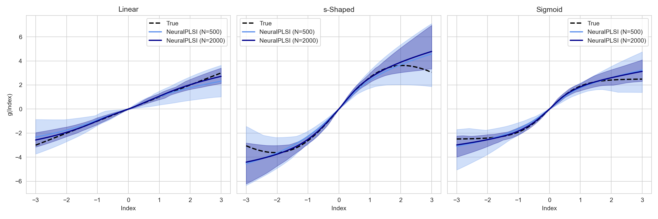
Figure 2 illustrates the estimated link functions using our proposed NeuralPLSI model and the B-spline approach described by Wang et al. (2020), along with their corresponding 95% confidence intervals. Even though both methods approximated the true unknown link functions well in both linear and nonlinear cases, a closer inspection of the plots reveals a key advantage of the NeuralPLSI model, particularly in capturing the tail behavior of the link functions. While the B-psline PLSI model performed well in the central range, it exhibits high variance and a less precise fit at the tails of the index values. In contrast, our proposed NeuralPLSI model demonstrated a more stable and accurate approximation in these tail regions, as evidenced by its narrower confidence intervals and closer alighnment with the true link function. This superior performance in the tails could be particularly important in applicaitons where extreme values of the predictor index are clinically or scientifically significant. For binary and survival outcomes, we observed similar simulation results of our proposed NeuralPLSI models, demonstrating empirically unbiased and reasonably efficient parameter estimates, along with well-approximated link functions (see Supplementary Materials).
3.2 NeuralPLSI Analysis of Triglycerdies: NHANES 2003–2004
| Covariates | NeuralPLSI | PLSI (Wang et al. (2020)) | |||
|---|---|---|---|---|---|
| Estimate | 95% CI | Estimate | 95% CI | ||
| Exposures | -Tocopherol | 0.526 | (0.481, 0.700) | 0.612 | (0.517, 0.707) |
| -Tocopherol | 0.298 | (0.255, 0.453) | 0.400 | (0.326, 0.475) | |
| Retinyl-palmitate | 0.368 | (0.175, 0.433) | 0.386 | (0.289, 0.484) | |
| Retinol | 0.220 | (0.103, 0.291) | 0.154 | (0.080, 0.228) | |
| 3,3,4,4,5-pncb | 0.165 | (0.042, 0.219) | 0.093 | (0.018, 0.168) | |
| PCB194 | -0.269 | (-0.381, -0.158) | -0.258 | (-0.377, -0.138) | |
| 2,3,4,6,7,8-hxcdf | -0.379 | (-0.427, -0.238) | -0.266 | (-0.345, -0.186) | |
| trans--carotene | -0.455 | (-0.501, -0.308) | -0.383 | (-0.456, -0.310) | |
| Confounders | Age | 0.006 | (0.002, 0.009) | 0.005 | (0.001, 0.010) |
| Sex | |||||
| Male | Ref | Ref | |||
| Female | -0.035 | (-0.176, 0.041) | -0.076 | (-0.167, 0.016) | |
| Race/Ethnicity | |||||
| Non-Hispanic White | Ref | Ref | |||
| Non-Hispanic Black | -0.203 | (-0.319, -0.059) | -0.138 | (-0.264, -0.011) | |
| Mexican American | 0.171 | (0.039, 0.291) | 0.175 | (0.054, 0.297) | |
| Other Race | 0.003 | (-0.128, 0.384) | 0.409 | (0.142, 0.676) | |
| Other Hispanic | 0.157 | (0.007, 0.429) | 0.355 | (0.083, 0.627) | |
For the continuous outcome of serum triglyceride concentration, the NeuralPLSI model identified both positive and negative associations between the eight environmental exposures and triglyceride levels (Table 2). The estimated link function was monotone increasing (Figure 3), indicating that the direction of each coefficient could be interpreted qualitatively in terms of its effect on mean triglyceride concentration.
Among the exposures, -tocopherol showed the strongest positive association (estimate = 0.526, 95% CI: 0.481 to 0.700), followed by retinyl palmitate (0.368, 95% CI: 0.175 to 0.433), -tocopherol (0.298, 95% CI: 0.255 to 0.453), retinol (0.220, 95% CI: 0.103 to 0.291), and 3,3’,4,4’,5-pentachlorobiphenyl (0.165, 95% CI: 0.042 to 0.219). In contrast, PCB194 (-0.269, 95% CI: -0.381 to -0.158), 2,3,4,6,7,8-hexachlorodibenzofuran (-0.379, 95% CI: -0.427 to -0.238), and trans--carotene (-0.455, 95% CI: -0.501 to -0.308) were negatively associated with triglyceride concentrations. For the confounders, age showed a small but statistically significant positive association (0.006, 95% CI: 0.002 to 0.009). Compared with non-Hispanic Whites, non-Hispanic Blacks (-0.203, 95% CI: -0.319 to -0.059) had significantly lower triglyceride levels. Additionally, Mexican Americans (0.171, 95% CI: 0.039 to 0.291) and Other Hispanics (0.157, 95% CI: 0.007 to 0.429) showed significant positive associations, while sex and Other Race contrasts showed no statistically significant associations in the NeuralPLSI analysis.
When compared with the results of spline-based PLSI on NHANES 2003–2004, following Wang et al. (2020), the overall pattern of associations was consistent in both direction and relative magnitude (Table 2). In both analyses, -tocopherol emerged as the strongest positive contributor to the index, while trans--carotene was the strongest negative contributor. The sign patterns for all eight exposures matched those reported by Wang et al. (2020), suggesting robust directional associations regardless of whether a spline-based or neural network-based link function was used. Differences were observed primarily in coefficient magnitudes: the NeuralPLSI estimates tended to be slightly larger in absolute value for the top-ranking exposures (- and -tocopherol, trans--carotene), possibly reflecting the model’s greater flexibility in capturing nonlinearities and complex interactions in the link function. The rank order of exposures by absolute coefficient size was identical between the two approaches, reinforcing the conclusion that the key drivers of triglyceride variability in this chemical mixture are largely consistent across modeling frameworks.
From an environmental health perspective, the positive associations for lipid-soluble antioxidants such as tocopherols and retinoids likely reflect their transport with triglyceride-rich lipoproteins. In contrast, the negative associations for POPs like PCB194, dioxin-like furans, and carotenoids may indicate more complex metabolic relationships or differential partitioning in lipid metabolism. The consistency between NeuralPLSI and spline-based PLSI results supports the robustness of these mixture–outcome relationships.

4 Discussion
We have developed a NeuralPLSI framework that unifies mixture analysis across common outcome types by combining an interpretable single exposure index with a learned nonlinear link. The approach preserves the dimensionality reduction and coefficient interpretability of classical single index models while adding flexibility through a neural link and scalability through stochastic optimization. A single training and inference pipeline adapts to continuous, categorical, and survival outcomes with modest changes that are limited to other mixture methods such as BKMR and WQS regression.
In our simulation study, NeuralPLSI provided a closer approximation to the true link functions than spline-based PLSI, particularly for nonlinear shapes such as S-shaped and sigmoid links at the extreme ends of the data. This demonstrates the advantage of a flexible neural network parameterization in capturing complex nonlinearities. However, the estimation of the index coefficients showed slightly higher variability (i.e., larger standard errors) with NeuralPLSI compared to spline-based PLSI. This likely arises because NeuralPLSI jointly estimates a highly flexible link function and the index coefficients, which increases the uncertainty in estimates. In contrast, spline-based PLSI uses a smoother, lower-dimensional representation of the link function, stabilizing estimation at the expense of potentially less accurate function approximation. Incorporating the covariance structure of exposures, with or without penalization, could improve the efficiency of estimates in the NeuralPLSI model, which we plan to explore in future work.
Methodologically, NeuralPLSI bridges the gap between predefined weighted sum approaches and fully nonparametric multivariate regressions. The single index provides a parsimonious and interpretable summary of the direction and relative magnitude of each exposure, while the learned link accommodates nonlinearity and interactions without manual basis design or pre-specification of interaction order. Compared with classical PLSI, NeuralPLSI reduces the tuning burden and scales naturally through minibatch optimization and automatic differentiation, which is particularly advantageous for larger cohorts and higher-dimensional exposure panels. Identifiability is enforced by constraining the index vector to unit norm with a fixed sign, and training is stabilized through standard regularization and early stopping. From a practical standpoint, the same objective function can incorporate case weights, facilitating the analysis of complex survey data when weighting is required. Post hoc visualizations of the fitted index response curve, together with confidence bands obtained via the bootstrap, further aid interpretation and model checking.
In the NHANES 2003–2004 case study of serum triglycerides modeled as a continuous outcome, NeuralPLSI identified mixed directional associations among the eight exposures. The strongest positive contribution was attributed to -tocopherol and the strongest negative contribution to trans -carotene, consistent with established biological relationships. The estimated link was close to linear over the observed index range, which explains the similarity between NeuralPLSI and its parametric counterpart in this application while preserving the capacity to deviate from linearity when supported by the data.
This study has several limitations and potential avenues for extension. Although the single index reduces dimensionality, learning a flexible link still requires a sufficient sample size and careful regularization. The estimated link trades some immediate transparency for adaptability; index response plots, shape constraints when scientifically justified, and sensitivity analyses can help mitigate this concern. Sparsity-inducing or structure-aware penalties on the index can improve performance with higher-dimensional exposure panels or known chemical groupings. Multiple index generalizations can capture distinct mechanistic pathways acting through different linear combinations of exposures. The common training and bootstrap inference pipeline supports reproducible practice and allows extensions to higher dimensions and multiple indices. For survival analysis, allowing time-varying links or interactions with time can relax the proportional hazards assumption while preserving the interpretability of the exposure index. Promising future directions also include work on transportability across cohorts, subgroup performance assessment, shape-constrained links informed by toxicology, and NeuralPLSI-based causal mediation analysis.
5 Conclusion
Evaluating the health effects of complex environmental mixtures is a persistent challenge in epidemiologic research. We developed the NeuralPLSI modeling framework to combine semiparametric interpretability with the flexibility of deep learning, enabling construction of an interpretable exposure index and modeling of its relationship with diverse outcome types. Simulation studies and application to NHANES data demonstrated its scalability, interpretability, and practical utility for mixture analyses. The accompanying open source software package facilitates adoption, reproducibility, and broader application in environmental health research.
Availability of data and materials
The data that support the findings in this paper are available from our previous study Wang et al. (2020). A user-friendly open-source software package for the proposed NeuralPLSI models is available at (https://github.com/hyungrok-do/NeuralPLSI).
Acknowledgement
This work was partially supported by NIH/NIEHS grant R01ES032808 and CDC grants U01OH012637 and R21OH012793.
References
- [1] (2012) Evaluation of biomonitoring data from the cdc national exposure report in a risk assessment context: perspectives across chemicals. Environmental health perspectives 121 (3), pp. 287. Cited by: §1.
- [2] (2018) Statistical software for analyzing the health effects of multiple concurrent exposures via bayesian kernel machine regression. Environmental Health 17 (1), pp. 67. Cited by: §1.
- [3] (2015) Bayesian kernel machine regression for estimating the health effects of multi-pollutant mixtures. Biostatistics 16 (3), pp. 493–508. Cited by: §1.
- [4] (2012) Serum triglycerides and risk of cardiovascular disease. Biochimica et Biophysica Acta (BBA)-Molecular and Cell Biology of Lipids 1821 (5), pp. 867–875. Cited by: §2.3.
- [5] (2016) What can epidemiological studies tell us about the impact of chemical mixtures on human health?. Environmental health perspectives 124 (1), pp. A6. Cited by: §1.
- [6] (2025) Prenatal phthalate exposure and anogenital distance in infants at 12 months. Environment international 199, pp. 109472. Cited by: §1.
- [7] (2015) Characterization of weighted quantile sum regression for highly correlated data in a risk analysis setting. Journal of agricultural, biological, and environmental statistics 20 (1), pp. 100–120. Cited by: §1, §1.
- [8] (2024) Evaluating associations of bisphenol and phthalate exposure with time to pregnancy and subfecundity in a new york city pregnancy cohort. Environmental Pollution 356, pp. 124281. Cited by: §1.
- [9] (2015-09–12 May) The Loss Surfaces of Multilayer Networks. In Proceedings of the Eighteenth International Conference on Artificial Intelligence and Statistics, G. Lebanon and S. V. N. Vishwanathan (Eds.), Proceedings of Machine Learning Research, Vol. 38, San Diego, California, USA, pp. 192–204. Cited by: Appendix B. Optimization and Inference.
- [10] (2013) Multiple classes of environmental chemicals are associated with liver disease: nhanes 2003–2004. International journal of hygiene and environmental health 216 (6), pp. 703–709. Cited by: §1.
- [11] (2020) Per-and poly-fluoroalkyl substances and bone mineral density: results from the bayesian weighted quantile sum regression. Environmental Epidemiology 4 (3), pp. e092. Cited by: §1.
- [12] (1972) Regression models and life-tables. Journal of the Royal Statistical Society: Series B (Methodological) 34 (2), pp. 187–202. Cited by: Appendix A. Extension of NeuralPLSI to Non-continuous Outcomes.
- [13] (2015) Assessment of weighted quantile sum regression for modeling chemical mixtures and cancer risk. Cancer informatics 14, pp. CIN–S17295. Cited by: §1.
- [14] (2014) Identifying and attacking the saddle point problem in high-dimensional non-convex optimization. Advances in neural information processing systems 27. Cited by: Appendix B. Optimization and Inference, Appendix B. Optimization and Inference.
- [15] (2022) Bayesian kernel machine regression-causal mediation analysis. Statistics in medicine 41 (5), pp. 860–876. Cited by: §1.
- [16] (2019) The association of urine metals and metal mixtures with cardiovascular incidence in an adult population from spain: the hortega follow-up study. International journal of epidemiology 48 (6), pp. 1839–1849. Cited by: §1.
- [17] (2015) Pilot study testing a european human biomonitoring framework for biomarkers of chemical exposure in children and their mothers: experiences in the uk. Environmental Science and Pollution Research 22 (20), pp. 15821–15834. Cited by: §1.
- [18] (2014) Human urinary excretion of non-persistent environmental chemicals: an overview of danish data collected between 2006 and 2012. Reproduction 147 (4), pp. 555–565. Cited by: §1.
- [19] (1989) On the approximate realization of continuous mappings by neural networks. Neural networks 2 (3), pp. 183–192. Cited by: §2.1.
- [20] (2013) A cohort study evaluation of maternal pcb exposure related to time to pregnancy in daughters. Environmental Health 12 (1), pp. 66. Cited by: §1.
- [21] (2018) Environmental exposure mixtures: questions and methods to address them. Current epidemiology reports 5 (2), pp. 160–165. Cited by: §1.
- [22] (1993) Optimal smoothing in single-index models. The annals of Statistics, pp. 157–178. Cited by: §1.
- [23] (1989) Investigating smooth multiple regression by the method of average derivatives. Journal of the American statistical Association 84 (408), pp. 986–995. Cited by: §1.
- [24] (2015) Delving deep into rectifiers: surpassing human-level performance on imagenet classification. In Proceedings of the IEEE international conference on computer vision, pp. 1026–1034. Cited by: Appendix B. Optimization and Inference.
- [25] (1997) Flat minima. Neural computation 9 (1), pp. 1–42. Cited by: Appendix B. Optimization and Inference.
- [26] (1989) Multilayer feedforward networks are universal approximators. Neural networks 2 (5), pp. 359–366. Cited by: §2.1.
- [27] (2006) Polynomial spline estimation and inference of proportional hazards regression models with flexible relative risk form. Biometrics 62 (3), pp. 793–802. Cited by: §1.
- [28] (1993) Semiparametric least squares (sls) and weighted sls estimation of single-index models. Journal of econometrics 58 (1-2), pp. 71–120. Cited by: §1.
- [29] (2017) Three factors influencing minima in sgd. arXiv preprint arXiv:1711.04623. Cited by: Appendix B. Optimization and Inference.
- [30] (2021) Partially linear single-index generalized mean residual life models. Statistics in medicine 40 (29), pp. 6707–6722. Cited by: §1.
- [31] (2022) Powering research through innovative methods for mixtures in epidemiology (prime) program: novel and expanded statistical methods. International Journal of Environmental Research and Public Health 19 (3), pp. 1378. Cited by: §1.
- [32] (2019) A quantile-based g-computation approach to addressing the effects of exposure mixtures. Environmental Epidemiology 3, pp. 44. Cited by: §1.
- [33] (2019) Early pregnancy exposure to endocrine disrupting chemical mixtures are associated with inflammatory changes in maternal and neonatal circulation. Scientific reports 9 (1), pp. 5422. Cited by: §1.
- [34] (2016) On large-batch training for deep learning: generalization gap and sharp minima. arXiv preprint arXiv:1609.04836. Cited by: Appendix B. Optimization and Inference.
- [35] (2014) Adam: a method for stochastic optimization. arXiv preprint arXiv:1412.6980. Cited by: Appendix B. Optimization and Inference.
- [36] (2007) Ten years of mixing cocktails: a review of combination effects of endocrine-disrupting chemicals. Environmental health perspectives 115 (Suppl 1), pp. 98. Cited by: §1.
- [37] (2024) Partial-linear single-index cox regression models with multiple time-dependent covariates. BMC Medical Research Methodology 24 (1), pp. 311. Cited by: §1.
- [38] (2024) Partial-linear single-index transformation models with censored data. Lifetime Data Analysis 30 (4), pp. 701–720. Cited by: §1.
- [39] (2025) Dynamic single-index scalar-on-function model. Statistics in Medicine 44 (10-12), pp. e70064. Cited by: §1.
- [40] (2010) Estimation and testing for partially linear single-index models. Annals of statistics 38 (6), pp. 3811. Cited by: §1.
- [41] (2021) Organophosphate pesticide exposure: demographic and dietary predictors in an urban pregnancy cohort. Environmental Pollution 283, pp. 116920. Cited by: §1.
- [42] (2022) Determinants of phthalate exposures in pregnant women in new york city. Environmental research 212, pp. 113203. Cited by: §1.
- [43] (2019) Generalized linear models. Routledge. Cited by: §2.1.
- [44] (2023) Bayesian multiple index models for environmental mixtures. Biometrics 79 (1), pp. 462–474. Cited by: §1, Appendix C. True Link Function Settings for Simulation Study.
- [45] (2011) Triglycerides and cardiovascular disease: a scientific statement from the american heart association. Circulation 123 (20), pp. 2292–2333. Cited by: §2.3.
- [46] (1972) Generalized linear models. Journal of the Royal Statistical Society Series A: Statistics in Society 135 (3), pp. 370–384. Cited by: §2.1.
- [47] (2017) Exploring generalization in deep learning. Advances in neural information processing systems 30. Cited by: Appendix B. Optimization and Inference.
- [48] (2016) GWQS: generalized weighted quantile sum regression. Cited by: §1.
- [49] (1986) A new approach to causal inference in mortality studies with a sustained exposure period—application to control of the healthy worker survivor effect. Mathematical modelling 7 (9-12), pp. 1393–1512. Cited by: §1.
- [50] (2015) Perinatal and childhood exposure to cadmium, manganese, and metal mixtures and effects on cognition and behavior: a review of recent literature. Current environmental health reports 2 (3), pp. 284–294. Cited by: §1.
- [51] (2013) Partially linear single index cox regression model in nested case-control studies. Computational statistics & data analysis 67, pp. 199–212. Cited by: §1.
- [52] (2012) The jackknife and bootstrap. Springer Science & Business Media. Cited by: Appendix B. Optimization and Inference.
- [53] (2017) Statistical approaches to address multi-pollutant mixtures and multiple exposures: the state of the science. Current environmental health reports 4 (4), pp. 481–490. Cited by: §1.
- [54] (2022) A review of environmental metabolism disrupting chemicals and effect biomarkers associating disease risks: where exposomics meets metabolomics. Environment International 158, pp. 106941. Cited by: §2.3.
- [55] (2008) Polynomial spline estimation of partially linear single-index proportional hazards regression models. Computational statistics & data analysis 53 (1), pp. 176–188. Cited by: §1.
- [56] (2020) Environmental mixtures and children’s health: identifying appropriate statistical approaches. Current opinion in pediatrics 32 (2), pp. 315–320. Cited by: §1.
- [57] (1993) An introduction to the bootstrap. Monographs on statistics and applied probability 57 (1), pp. 1–436. Cited by: Appendix B. Optimization and Inference.
- [58] (2020) Prenatal exposure to a mixture of persistent organic pollutants (pops) and child reading skills at school age. International journal of hygiene and environmental health 228, pp. 113527. Cited by: §1.
- [59] (2023) Semiparametric distributed lag quantile regression for modeling time-dependent exposure mixtures. Biometrics 79 (3), pp. 2619–2632. Cited by: §1.
- [60] (2020) A family of partial-linear single-index models for analyzing complex environmental exposures with continuous, categorical, time-to-event, and longitudinal health outcomes. Environmental Health 19 (1), pp. 96. Cited by: §1, §1, §2.2, §2.3, §2.3, §3.1, §3.2, Table 2, Table 2, Availability of data and materials.
- [61] (2005) Complementing the genome with an “exposome”: the outstanding challenge of environmental exposure measurement in molecular epidemiology. Cancer Epidemiology Biomarkers & Prevention 14 (8), pp. 1847–1850. Cited by: §1.
- [62] (2002) Penalized spline estimation for partially linear single-index models. Journal of the American Statistical Association 97 (460), pp. 1042–1054. Cited by: §1.
Appendix
Appendix A. Extension of NeuralPLSI to Non-continuous Outcomes
The NeuralPLSI model can be naturally extended beyond continuous outcomes by introducing a suitable link function that connects the expected response to the additive model components. This generalization places NeuralPLSI within the broader family of generalized neural network-based partial-linear single-index models, allowing its application to binary, count, and time-to-event outcomes.
In generalized linear models (GLMs), the conditional mean of the response variable given covariates is linked to a linear predictor through a monotonic, differentiable link function . We extend this principle to our framework by modeling
| (3) |
where is the inverse link function appropriate for the distribution of . This formulation allows us to retain the flexible, nonparametric modeling of the index component , while incorporating outcome-specific characteristics through .
For example, when , a common choice is the logistic link , leading to a semiparametric single-index logistic regression:
| (4) |
For Poisson-distributed , we use a log link , yielding
| (5) |
The optimization problem in this setting becomes the maximization of a generalized log-likelihood:
| (6) |
where is the conditional density or probability mass function of under its assumed distribution (e.g., Bernoulli or Poisson).
The NeuralPLSI framework can also be extended to time-to-event data using the Cox proportional hazards model [12]. The survival variant fit naturally into the framework by embedding the single index within a proportional hazards formulation, allowing partial likelihood training with the same identifiability constraints and regularization. In this context, we model the hazard function as
| (7) |
where is the baseline hazard function and the index-based nonlinear transformation replaces the usual linear predictor in standard Cox models. The model retains the proportional hazards structure while permitting nonlinear interactions among through the learned index.
Given a dataset with covariates , observed times , and event indicators , we maximize the partial log-likelihood as:
| (8) |
where denotes the risk set at time . This model enables flexible modeling of survival data with both interpretable linear effects and complex nonlinear components. We further note that this can easily be extended to the accelerated failure time framework or nonparametric survival models.
Appendix B. Optimization and Inference
Because the objective function of NeuralPLSI involves a composition of a nonlinear neural network with parameters and a learnable projection vector , the resulting optimization problem is highly non-convex. This non-convexity stems from multiple sources. First, the neural network introduces complex, non-linear mappings that can lead to a highly non-convex loss surface with many local minima and saddle points [9, 14]. Second, the interaction between the neural network and the index direction compounds this complexity. Since the output of the neural network depends on the projection , the loss is sensitive not only to the orientation of but also to the internal structure of , creating a coupled optimization landscape.
To solve this type of problem, stochastic gradient descent (SGD) and its variants, such as Adam [35], are popularly used. These methods are widely recognized as effective for optimizing deep neural networks with highly non-convex objectives. Unlike full-batch gradient descent, which computes gradients over the entire dataset at each iteration, SGD uses randomly sampled minibatches to estimate the gradient direction. This stochasticity serves two crucial purposes. First, it drastically reduces memory consumption, making training feasible in large-scale datasets and resource-constrained environments. Second, and more importantly, in the context of the NeuralPLSI, the inherent noise introduced by minibatch updates acts as a regularizer that helps the optimizer escape poor local minima and saddle points. In high-dimensional non-convex landscapes, saddle points, where gradients vanish but the point is not a local minimum, are far more prevalent than local minima and often pose significant obstacles to optimization [14]. Full-batch gradient descent can become stuck near such saddle points because of vanishing gradients and the curvature being flat in some directions and negative in others. SGD, by contrast, introduces sufficient perturbations through minibatch noise to break symmetry and escape these degenerate regions, allowing continued progress toward lower loss values. Moreover, non-convex loss surfaces often contain multiple local minima, some of which are sharp and narrow, while others are flat and wide. Sharp minima correspond to solutions with high curvature, where small changes in parameters can lead to large changes in loss, often resulting in poor generalization. Flat minima, on the other hand, tend to be more robust and yield better generalization performance [25, 34]. The stochasticity in SGD biases the search trajectory toward flatter regions of the loss surface, improving the generalizability and stability of the model [29, 47]. These characteristics make stochastic optimization particularly well-suited for NeuralPLSI, where the composition of a nonlinear neural network and a learnable projection direction creates a highly coupled and rugged loss surface. The ability of SGD and its adaptive variants to escape saddle points, avoid sharp minima, and promote generalizable solutions is essential for reliable training in such settings.
Training of neural networks is sensitive to initialization, and poor initialization can lead to slow convergence or suboptimal solutions. We use standard initialization schemes such as He initialization [24] to ensure that the variance of activations is preserved across layers, thereby stabilizing gradient propagation during early training epochs.
During training, the model parameters are jointly updated via gradient-based optimization to minimize a loss function, typically mean squared error or negative log-likelihood, depending on the outcome type. After each gradient update, we re-normalize the vector to enforce the constraint and flip the signs of if . This constraint is essential for identifiability: without it, arbitrary rescaling between and the input to could yield the same overall model behavior but with different parameter values.
In summary, the training of NeuralPLSI models integrates (i) stochastic minibatch updates for memory-efficient and noise-assisted optimization, (ii) adaptive optimizers for scale-aware learning, (iii) careful weight initialization to preserve stability, and (iv) constraint enforcement for identifiability. This combination allows effective learning even in complex and high-dimensional data regimes.
Conventional statistical models such as linear regression, GLMs, and Cox proportional hazards models permit formal statistical inference on model parameters through asymptotic theory. However, in the NeuralPLSI framework, inference is considerably more challenging due to the nonparametric nature of the neural network component and the absence of closed-form MLEs.
The NeuralPLSI model has the general form where and are learnable linear parameters, and is a nonlinear function modeled via a neural network. Despite extensive progress in quantifying predictive uncertainty in neural networks, such as MC dropout, SWAG, and Laplace approximations, these approaches do not directly yield standard errors or confidence intervals for and . Analytical variance estimation is further complicated by the lack of a well-specified likelihood and the interdependence of , , and in the optimization process.
Therefore, to enable inference of the parametric components and , we adopt a nonparametric bootstrap procedure (Algorithm 2). This approach is model-agnostic and accommodates the complexities inherent to neural network optimization. Let and denote the parameter estimates obtained by fitting the NeuralPLSI model to the complete dataset .
Confidence intervals for each component can be obtained via the bootstrap percentile method or by assuming approximate normality. For the -th component of , the confidence interval is given by
| (9) |
and similarly, for the -th component of , the confidence interval is
| (10) |
where is the -quantile of the standard normal distribution, and denotes the desired significance level (e.g., for a confidence interval).
The above inference procedure generalizes naturally to variants of the NeuralPLSI model involving non-continuous responses, such as those modeled via GLM or Cox proportional hazards models. In such settings, the linear component and the nonlinear index are combined within appropriate link or hazard functions, and inference on can still be validly conducted using nonparametric bootstrap methods [57, 52]. This bootstrap-based approach enables robust estimation of uncertainty in partially linear models involving neural networks. It is flexible, easy to implement, and does not require explicit modeling assumptions about the distribution of the estimators. Moreover, it provides valid inference for both linear and nonlinear components across continuous, discrete, and censored outcome settings.
Appendix C. True Link Function Settings for Simulation Study
In our simulation study, we assumed one linear and two nonlinear link functions as follows. was assumed to be a S-shaped function, that is, . was assumed as a sigmoidal function, . These two shape functions were refereed from the simulation setting of [44]. We provided the shapes of each nonlinear function in Figure 4.

Appendix D. Additional Simulation Results
Table 1 presents the simulation results for a continuous outcome with . Both NeuralPLSI and PLSI models performed similarly, yielding empirically unbiased estimates and reasonable efficiency. Compared to the results for (Table 1 and Figure 2 of the manuscript), SD and SE increased, resulting in slightly underperformed CP relative to the 95% nominal level, as expected. Similar patterns were observed for the binary and survival outcomes (Tables 2–4 and Figures 3–5).
| -function | Parameter | NeuralPLSI () | NeuralPLSI () | ||||||
|---|---|---|---|---|---|---|---|---|---|
| Bias | SD | SE | CP | Bias | SD | SE | CP | ||
| Linear | -0.0144 | 0.0475 | 0.0534 | 0.9800 | -0.0047 | 0.0240 | 0.0220 | 0.9600 | |
| -0.0107 | 0.0507 | 0.0611 | 1.0000 | -0.0018 | 0.0264 | 0.0265 | 0.9800 | ||
| 0.0085 | 0.0694 | 0.0581 | 0.9400 | -0.0013 | 0.0257 | 0.0254 | 1.0000 | ||
| 0.0065 | 0.0558 | 0.0645 | 1.0000 | 0.0008 | 0.0326 | 0.0282 | 0.9200 | ||
| 0.0022 | 0.0824 | 0.0664 | 0.9800 | 0.0003 | 0.0298 | 0.0292 | 0.9800 | ||
| -0.0006 | 0.0615 | 0.0642 | 1.0000 | -0.0043 | 0.0258 | 0.0286 | 0.9600 | ||
| -0.0094 | 0.0618 | 0.0652 | 0.9600 | -0.0015 | 0.0301 | 0.0288 | 0.9800 | ||
| 0.0012 | 0.0604 | 0.0653 | 0.9800 | -0.0013 | 0.0254 | 0.0291 | 0.9800 | ||
| -0.0939 | 0.0529 | 0.0997 | 0.8400 | -0.0084 | 0.0247 | 0.0252 | 0.9400 | ||
| 0.0119 | 0.0398 | 0.0578 | 1.0000 | 0.0010 | 0.0249 | 0.0252 | 0.9800 | ||
| -0.0073 | 0.0458 | 0.0571 | 0.9800 | -0.0020 | 0.0280 | 0.0250 | 0.9400 | ||
| s-Shape | -0.0037 | 0.0203 | 0.0248 | 0.9600 | -0.0005 | 0.0101 | 0.0098 | 0.9400 | |
| -0.0023 | 0.0209 | 0.0343 | 1.0000 | -0.0015 | 0.0111 | 0.0119 | 1.0000 | ||
| 0.0007 | 0.0298 | 0.0293 | 0.9400 | 0.0002 | 0.0101 | 0.0114 | 1.0000 | ||
| 0.0032 | 0.0234 | 0.0336 | 0.9800 | 0.0020 | 0.0131 | 0.0127 | 0.9600 | ||
| 0.0004 | 0.0351 | 0.0318 | 0.9600 | -0.0012 | 0.0143 | 0.0130 | 0.9600 | ||
| 0.0020 | 0.0253 | 0.0307 | 1.0000 | -0.0015 | 0.0107 | 0.0127 | 0.9600 | ||
| -0.0044 | 0.0293 | 0.0300 | 0.9400 | 0.0002 | 0.0143 | 0.0130 | 0.9800 | ||
| 0.0025 | 0.0267 | 0.0304 | 0.9800 | -0.0019 | 0.0124 | 0.0130 | 0.9800 | ||
| -0.0941 | 0.0492 | 0.0992 | 0.8800 | -0.0081 | 0.0263 | 0.0255 | 0.9600 | ||
| 0.0138 | 0.0408 | 0.0584 | 1.0000 | 0.0008 | 0.0247 | 0.0252 | 0.9800 | ||
| -0.0101 | 0.0453 | 0.0581 | 0.9800 | -0.0018 | 0.0277 | 0.0251 | 0.9400 | ||
| Sigmoid | -0.0057 | 0.0266 | 0.0317 | 0.9800 | -0.0005 | 0.0142 | 0.0135 | 0.9600 | |
| -0.0032 | 0.0292 | 0.0394 | 1.0000 | -0.0024 | 0.0154 | 0.0163 | 1.0000 | ||
| 0.0042 | 0.0408 | 0.0362 | 0.9400 | 0.0012 | 0.0141 | 0.0156 | 1.0000 | ||
| 0.0037 | 0.0331 | 0.0409 | 0.9800 | 0.0026 | 0.0180 | 0.0175 | 0.9400 | ||
| 0.0012 | 0.0493 | 0.0414 | 0.9600 | -0.0010 | 0.0199 | 0.0179 | 0.9800 | ||
| 0.0029 | 0.0357 | 0.0400 | 1.0000 | -0.0027 | 0.0152 | 0.0175 | 0.9600 | ||
| -0.0062 | 0.0415 | 0.0397 | 0.9400 | -0.0008 | 0.0189 | 0.0178 | 0.9800 | ||
| 0.0023 | 0.0387 | 0.0402 | 0.9800 | -0.0027 | 0.0169 | 0.0179 | 0.9800 | ||
| -0.1026 | 0.0501 | 0.1013 | 0.8600 | -0.0109 | 0.0255 | 0.0254 | 0.9400 | ||
| 0.0146 | 0.0402 | 0.0576 | 1.0000 | 0.0014 | 0.0245 | 0.0252 | 0.9800 | ||
| -0.0093 | 0.0445 | 0.0573 | 0.9800 | -0.0023 | 0.0276 | 0.0250 | 0.9400 | ||

| -function | Parameter | NeuralPLSI () | NeuralPLSI () | ||||||
|---|---|---|---|---|---|---|---|---|---|
| Bias | SD | SE | CP | Bias | SD | SE | CP | ||
| Linear | -0.0934 | 0.1643 | 0.1514 | 0.9400 | -0.0227 | 0.0506 | 0.0562 | 0.9800 | |
| -0.0693 | 0.1555 | 0.1820 | 1.0000 | 0.0039 | 0.0624 | 0.0661 | 1.0000 | ||
| 0.1231 | 0.2139 | 0.1761 | 0.9600 | 0.0030 | 0.0702 | 0.0641 | 0.9800 | ||
| -0.0408 | 0.2407 | 0.1829 | 1.0000 | -0.0017 | 0.0824 | 0.0701 | 0.9600 | ||
| 0.0147 | 0.1724 | 0.1743 | 1.0000 | -0.0137 | 0.0692 | 0.0725 | 0.9800 | ||
| 0.0253 | 0.1667 | 0.1721 | 1.0000 | 0.0032 | 0.0618 | 0.0726 | 1.0000 | ||
| 0.0012 | 0.1425 | 0.1742 | 1.0000 | -0.0012 | 0.0595 | 0.0733 | 1.0000 | ||
| 0.0068 | 0.2208 | 0.1736 | 1.0000 | 0.0041 | 0.0814 | 0.0720 | 0.9200 | ||
| -0.3248 | 0.1741 | 0.1924 | 0.6000 | -0.0449 | 0.0689 | 0.0780 | 0.9800 | ||
| 0.1407 | 0.1270 | 0.1337 | 0.9400 | 0.0077 | 0.0661 | 0.0635 | 0.9600 | ||
| -0.1240 | 0.1475 | 0.1337 | 0.9000 | -0.0123 | 0.0704 | 0.0622 | 1.0000 | ||
| s-Shaped | -0.0156 | 0.1037 | 0.0749 | 0.9600 | -0.0066 | 0.0184 | 0.0253 | 0.9800 | |
| -0.0265 | 0.0627 | 0.0902 | 1.0000 | -0.0009 | 0.0221 | 0.0306 | 1.0000 | ||
| 0.0205 | 0.0703 | 0.0807 | 1.0000 | -0.0059 | 0.0278 | 0.0289 | 0.9800 | ||
| -0.0034 | 0.1377 | 0.0897 | 0.9800 | -0.0012 | 0.0332 | 0.0323 | 0.9600 | ||
| -0.0125 | 0.0928 | 0.0827 | 0.9600 | 0.0007 | 0.0306 | 0.0338 | 1.0000 | ||
| 0.0078 | 0.0746 | 0.0813 | 1.0000 | 0.0030 | 0.0340 | 0.0336 | 1.0000 | ||
| 0.0033 | 0.0728 | 0.0823 | 1.0000 | 0.0030 | 0.0338 | 0.0333 | 0.9800 | ||
| -0.0070 | 0.1078 | 0.0822 | 1.0000 | 0.0024 | 0.0317 | 0.0333 | 0.9800 | ||
| -0.3545 | 0.1379 | 0.2049 | 0.5800 | -0.0789 | 0.0903 | 0.0931 | 0.9000 | ||
| 0.1488 | 0.1142 | 0.1510 | 0.9600 | 0.0199 | 0.0755 | 0.0775 | 1.0000 | ||
| -0.1585 | 0.1170 | 0.1490 | 0.9000 | -0.0146 | 0.0838 | 0.0768 | 0.9800 | ||
| Sigmoid | -0.0114 | 0.0690 | 0.0981 | 0.9800 | -0.0071 | 0.0281 | 0.0332 | 0.9800 | |
| -0.0449 | 0.0885 | 0.1163 | 1.0000 | 0.0052 | 0.0315 | 0.0396 | 1.0000 | ||
| 0.0518 | 0.0999 | 0.1082 | 1.0000 | 0.0012 | 0.0396 | 0.0376 | 0.9600 | ||
| 0.0278 | 0.1119 | 0.1160 | 1.0000 | -0.0093 | 0.0462 | 0.0427 | 0.9600 | ||
| 0.0015 | 0.0963 | 0.1097 | 0.9800 | 0.0022 | 0.0332 | 0.0439 | 1.0000 | ||
| -0.0109 | 0.0906 | 0.1081 | 0.9800 | 0.0053 | 0.0417 | 0.0436 | 0.9800 | ||
| 0.0165 | 0.0902 | 0.1096 | 0.9800 | 0.0014 | 0.0376 | 0.0435 | 0.9800 | ||
| -0.0160 | 0.0899 | 0.1102 | 0.9800 | -0.0025 | 0.0475 | 0.0428 | 0.9600 | ||
| -0.3278 | 0.0846 | 0.1974 | 0.5800 | -0.0696 | 0.0747 | 0.0838 | 0.9200 | ||
| 0.1260 | 0.0915 | 0.1433 | 0.9200 | 0.0142 | 0.0662 | 0.0693 | 0.9600 | ||
| -0.1287 | 0.1030 | 0.1397 | 0.8800 | -0.0078 | 0.0736 | 0.0686 | 0.9800 | ||
| -function | Parameter | NeuralPLSI () | NeuralPLSI () | ||||||
|---|---|---|---|---|---|---|---|---|---|
| Bias | SD | SE | CP | Bias | SD | SE | CP | ||
| Linear | -0.0264 | 0.0728 | 0.1217 | 1.0000 | -0.0060 | 0.0337 | 0.0322 | 0.9400 | |
| -0.0149 | 0.0818 | 0.1457 | 1.0000 | 0.0022 | 0.0408 | 0.0381 | 0.9400 | ||
| 0.0403 | 0.1137 | 0.1369 | 0.9200 | -0.0007 | 0.0425 | 0.0360 | 0.9600 | ||
| 0.0194 | 0.1024 | 0.1435 | 1.0000 | -0.0074 | 0.0416 | 0.0401 | 0.9800 | ||
| -0.0359 | 0.0864 | 0.1316 | 1.0000 | -0.0054 | 0.0383 | 0.0421 | 1.0000 | ||
| -0.0086 | 0.1034 | 0.1296 | 1.0000 | 0.0022 | 0.0416 | 0.0409 | 1.0000 | ||
| 0.0022 | 0.0992 | 0.1312 | 0.9800 | 0.0031 | 0.0441 | 0.0417 | 0.9400 | ||
| -0.0005 | 0.1142 | 0.1305 | 1.0000 | -0.0007 | 0.0457 | 0.0419 | 0.9400 | ||
| -0.2094 | 0.0837 | 0.1695 | 0.7200 | -0.0437 | 0.0433 | 0.0472 | 0.9400 | ||
| 0.0810 | 0.0772 | 0.0997 | 0.8600 | 0.0131 | 0.0406 | 0.0380 | 1.0000 | ||
| -0.0775 | 0.0793 | 0.0992 | 0.8600 | -0.0104 | 0.0332 | 0.0382 | 0.9800 | ||
| s-Shaped | -0.0258 | 0.1222 | 0.0643 | 0.9800 | -0.0013 | 0.0143 | 0.0144 | 0.9600 | |
| -0.0308 | 0.1474 | 0.0842 | 0.9800 | -0.0002 | 0.0160 | 0.0175 | 0.9800 | ||
| 0.0382 | 0.1812 | 0.0717 | 1.0000 | 0.0004 | 0.0200 | 0.0164 | 0.9600 | ||
| 0.0072 | 0.0583 | 0.0760 | 1.0000 | -0.0014 | 0.0177 | 0.0184 | 0.9600 | ||
| -0.0075 | 0.0407 | 0.0667 | 0.9800 | 0.0013 | 0.0185 | 0.0190 | 1.0000 | ||
| -0.0059 | 0.0450 | 0.0594 | 1.0000 | -0.0005 | 0.0209 | 0.0185 | 0.9600 | ||
| 0.0025 | 0.0444 | 0.0633 | 1.0000 | 0.0019 | 0.0177 | 0.0189 | 0.9600 | ||
| -0.0166 | 0.0949 | 0.0621 | 1.0000 | -0.0001 | 0.0205 | 0.0189 | 0.9400 | ||
| -0.2446 | 0.1678 | 0.1636 | 0.6200 | -0.0543 | 0.0432 | 0.0491 | 0.9400 | ||
| 0.1108 | 0.1208 | 0.1001 | 0.8400 | 0.0194 | 0.0355 | 0.0396 | 0.9800 | ||
| -0.1074 | 0.1214 | 0.0991 | 0.8200 | -0.0143 | 0.0325 | 0.0393 | 0.9800 | ||
| Sigmoid | -0.0297 | 0.1135 | 0.0758 | 0.9800 | -0.0025 | 0.0188 | 0.0196 | 0.9400 | |
| -0.0166 | 0.1020 | 0.0951 | 0.9600 | -0.0006 | 0.0230 | 0.0238 | 0.9600 | ||
| 0.0253 | 0.1336 | 0.0849 | 1.0000 | 0.0011 | 0.0263 | 0.0222 | 0.9600 | ||
| -0.0066 | 0.1235 | 0.0896 | 1.0000 | -0.0009 | 0.0254 | 0.0250 | 0.9400 | ||
| -0.0151 | 0.0718 | 0.0801 | 0.9800 | 0.0013 | 0.0250 | 0.0261 | 1.0000 | ||
| -0.0032 | 0.0788 | 0.0755 | 1.0000 | 0.0001 | 0.0285 | 0.0252 | 0.9600 | ||
| 0.0046 | 0.0669 | 0.0779 | 0.9800 | 0.0022 | 0.0260 | 0.0257 | 0.9400 | ||
| 0.0005 | 0.1118 | 0.0770 | 1.0000 | -0.0005 | 0.0273 | 0.0259 | 0.9400 | ||
| -0.2370 | 0.1580 | 0.1637 | 0.7200 | -0.0485 | 0.0423 | 0.0479 | 0.9400 | ||
| 0.1045 | 0.1132 | 0.0963 | 0.9000 | 0.0151 | 0.0403 | 0.0386 | 1.0000 | ||
| -0.1035 | 0.1121 | 0.0972 | 0.8600 | -0.0100 | 0.0310 | 0.0387 | 0.9800 | ||
