Ginwidth=\Gin@nat@width,height=\Gin@nat@height,keepaspectratio
Asymptotic Uniform False Discovery Rate Control for Inference of Time-varying Correlations
Abstract
Inference for locally stationary time series is challenging because the associated hypotheses form an uncountable collection over a continuous time interval, making pointwise false discovery rate (FDR) control inadequate for simultaneous statistical guarantees. We introduce a novel asymptotically uniform false discovery rate (AuFDR), defined as the expectation of the -norm of the false discovery proportion (FDP) process where is allowed to diverge, to quantify and control false discoveries uniformly over time. To operationalize AuFDR control, we develop an inferential framework for time-varying correlations in high-dimensional nonstationary time series that allows for non-Gaussianity, nonlinearity and possible jumps in mean functions. The proposed approach combines robust difference-based estimators with a multiplier-bootstrap procedure to construct uniformly valid time-varying -values. Based on these -values, we propose a time-varying Benjamini–Yekutieli procedure for controlling the AuFDR under arbitrary dependence and establish its asymptotic validity. Extensive simulations demonstrate the finite-sample performance of the proposed method in controlling the AuFDR. Applications to EEG data and financial time-series data illustrate its practical utility.
Keywords: time-varying correlation, locally stationary time series, high-dimensional inference, multiplier bootstrap, asymptotic uniform false discovery rate
1 Introduction
A standard approach of error control in large-scale testing is false discovery rate (FDR) control (Benjamini and Yekutieli 2001). In the analysis of non-stationary time series under a time-varying scheme, however, additional challenges arise when the hypotheses are indexed by a continuous time parameter, yielding an uncountable family of tests. For instance, in the inference of time-varying correlations (see Hutchison et al. (2013), Lurie et al. (2020) in neuroscience and Onnela et al. (2003), Marti et al. (2021) in finance as examples), one is interested in testing the null hypothesis of zero correlation for each pair at each rescaled time point , yielding a family of hypotheses indexed by both pairs and time. As an example, Figure 1 illustrates such an approach on an EEG dataset (Zhang et al. 1997).

To conduct reliable inference on non-stationary time series under a time-varying scheme, one needs error control that accounts for the entire trajectory of the time-varying false discovery proportion, . Conventional pointwise FDR procedures control only at each fixed time point . As illustrated by the simulation results in Section 5.3, such pointwise control methods cannot guarantee that the time-varying FDPs are low globally. Therefore, pointwise error control does not provide global inferential validity for multiple testing in a time-varying framework, and a uniform error criterion is therefore needed.

The supremum-based criterion is a natural worst-case benchmark, but it is not always well aligned with time-varying inference based on local smoothing. For example, suppose the underlying process undergoes an abrupt transition at time , moving from a regime with dense and large enough signals to a global null regime. In that case, tests based on local estimators may continue to reject some null hypotheses immediately after because data from the pre-change region will leak into the post-change estimates. The may equal one even when false discoveries are well-controlled over nearly the entire interval. This distinction is illustrated in Figure 2.
To address this issue, we introduce the asymptotically uniform false discovery rate (AuFDR), which can be viewed as a regularized version of the supremum FDP criterion. For any fixed , define For a pre-specified sequence , we define
Since approaches as , the criterion retains a uniform interpretation. At the same time, the use of an -norm avoids the excessive sensitivity to isolated local spikes. To illustrate this, suppose that outside a transition set with Lebesgue measure , the FDP process is bounded by , whereas within it may be as large as one. Then
Consequently, if , the influence of the transition set vanishes asymptotically. In contrast, remains uncontrolled whenever such a spike occurs. Thus, by employing a slowly diverging and user-specified value of , the proposed captures the global behavior of the FDP process while reducing sensitivity to local signal irregularities.
To illustrate the utility of this new framework, we develop an AuFDR control procedure for testing the null hypotheses of zero correlations over the rescaled time interval . The framework is designed for high-dimensional locally stationary time series and accommodates features common in neuroimaging (Lurie et al. 2020) and financial data (Jondeau et al. 2007, De Domenico et al. 2023), including mean discontinuities, non-Gaussianity, nonlinearity, and nonstationarity.
To guarantee AuFDR control for this testing problem, we first construct time-varying -values that are uniformly valid. The construction combines robust difference-based estimators with a multiplier bootstrap procedure. The difference-based estimators reduce sensitivity to unknown and potentially discontinuous mean functions, while the multiplier bootstrap approximates the maximum deviation of the relevant high-dimensional time-varying test statistics. Given these uniformly valid time-varying -values, we develop a time-varying Benjamini–Yekutieli (BY) procedure for time-varying multiple testing. The procedure applies the BH step at the adjusted nominal level , where , to account for arbitrary dependence. We show that the resulting procedure controls the asymptotically with .
Our theoretical contribution is a new hyperrectangle Gaussian approximation result for high-dimensional second-order structures of locally stationary processes. Existing Gaussian approximation results for locally stationary time series primarily focus on first-order statistics (Zhang and Cheng 2018, Chang et al. 2024). Some recent work has begun to address second-order structures with maximum type Gaussian approximation results, see Ding and Zhou (2020) and Zhang et al. (2024) for examples. In contrast, correlation inference involves products of variables and therefore requires approximating the distribution of high-dimensional product processes over time. A related maximum-type approximation was developed by Bai and Wu (2025) for uniform FWER control to obtain a single global threshold for the bootstrap method. However, in the present AuFDR framework, the time-varying BY procedure requires the simultaneous validity of all -values, which naturally leads to Gaussian approximation over high-dimensional hyperrectangles. We establish such an approximation result and use it to prove the uniform validity of the proposed time-varying -values, subsequently enabling us to establish AuFDR control for the time-varying BY procedure. Zhang et al. (2024), Ding and Zhou (2020)
1.1 Related work on correlation testing and FDR control.
Large-scale correlation testing has been extensively studied with time-invariant inference results (Efron 2007, Cai and Liu 2016, Bailey et al. 2019). These methods, however, are not designed for settings in which the correlation structure evolves over time. Recent work has addressed time-varying correlation inference with uniform family-wise error rate (FWER) control (Bai and Wu 2025), but FDR-based control for time-varying correlation tests remains largely unexplored.
There is also a rich literature on FDR control under dependence (Benjamini and Yekutieli 2001, Barber and Candès 2015, Fithian and Lei 2022). Nevertheless, inference for time-varying correlations for high-dimensional and locally stationary time series via multiple testing with FDR control poses several difficulties that are not covered by existing results. These include that (a) The underlying process is nonstationary, which leads to intricate limiting distributions of the test statistics that complicate testing the corresponding hypothesis. Moreover, the number of hypotheses diverges with dimension growing, which further sophisticates the joint distribution of the -values. (b) The time-varying -values obtained in this setting exhibits complicated cross-sectional dependence across pairs together with intricate temporal dependence across the time index, which brings further difficulties on FDR control. These features require a new analytical framework beyond existing results.
| Notation | Expression |
|---|---|
| the observation, innovation and trend function in (1) | |
| Lag parameter in the difference-based method | |
| local linear estimators from (5) | |
| Estimator for pairwise covariance: | |
| Estimator for marginal covariance: | |
| Estimator for pairwise correlation: |
| Notation | Expression |
|---|---|
| Residuals of the regression in (5): | |
| The limiting variance of | |
| , , | |
| i.i.d. random variables used in multiplier bootstrap | |
The rest of the paper is organized as follows. Section 2 formulates the testing problem and defines the AuFDR criterion. Section 3 presents the proposed methodology, including the difference-based estimator, the multiplier bootstrap procedure, and the time-varying BY procedure. Section 4 establishes the theoretical guarantees, including the uniform validity of the time-varying -values and asymptotic AuFDR control. Sections 5 and 6 report simulation studies and real-data applications, respectively. Section 9 contains the data availability statement. All technical proofs are delegated to the Appendix. In Table 1 we list some notations used in time-varying correlation estimation in Section 3.1. In Table 2 we list the notations used in the inference procedure in Section 3.2 and 3.3.
2 Preliminaries
Notations. For a positive integer , let . For a vector , let , . For two vectors , write if for all . For a random vector and , let . For a measurable function on , we define its -norm as . Throughout this paper, denotes a kernel function with support , and we define for a bandwidth . For any set , denotes its cardinality.
2.1 High-dimensional Locally Stationary Time Series with Jumps in Mean
We consider a -dimensional time series with the following model
| (1) |
where is the rescaled observation time, is the deterministic mean function, and is the stochastic error process. The error process is assumed to be a non-Gaussian, nonlinear and locally stationary time series, and we consider a high-dimensional regime in which the dimension is allowed to grow with the sample size . For mean functions, we suppose that has jumps:
where are the jump locations for the th component. On each , the function is assumed to be Lipschitz continuous, with Lipschitz constants uniformly bounded over and . We allow to grow with , corresponding to a regime of dense jumps.
Model (1) also covers the special case of globally smooth mean functions with no structural breaks (i.e., ). We focus on the more challenging setting where , while the case can be treated similarly.
2.2 Uniform Inference of Correlations and AuFDR
For , define the time-varying covariance , marginal variance , and correlation by
We consider testing, for each and each , the hypotheses
| (2) |
Let denote the set of rejected hypotheses at time , and let denote the set of true null hypotheses. The FDP at time is defined by
| (3) |
To provide simultaneous error control over the entire FDP trajectory, we define the AuFDR as
| (4) |
where is a sequence of parameters chosen by the user. Our goal is to develop a procedure that controls at a prescribed level.
Remark 1 (Network visualization).
The proposed framework naturally yields a time-varying correlation network , where is the vertex set, and the time-varying edge set represents pairs with statistically significant nonzero correlation.
Remark 2 (Other hypothesis testing problems).
While we focus on testing the null hypothesis of zero correlation as defined in (2), the proposed framework can be readily extended to other hypotheses. For instance, one could test , where is any given measurable function.
Remark 3 (Difficulty of controlling AuFDR).
Controlling is more challenging than obtaining pointwise FDR control over local windows, because pointwise control of the FDP does not imply control of the -norm of the time-varying FDP when . By comparison, our inference procedure can control .
3 Methodology
3.1 Difference-based Correlation Estimation Method
To estimate the time-varying correlation function in the presence of abrupt jumps in means, we adopt a difference-based approach in Bai and Wu (2025). Let be a sequence of integers such that and . For and , define . Under the assumption that the temporal dependence of the error process decays fast enough as the lag increases, we have , which implies . Furthermore, provided the trend function is piecewise Lipschitz and the lag is sufficiently small relative to , the differenced observations effectively filter out the mean trend: , except in the vicinity of a jump.
Based on the analysis above, we estimate by the local linear estimator , with
| (5) |
where is the bandwidth parameter. To simplify notation, we suppress the dependence of the estimator on . The choice of is discussed in Section 3.5. The time-varying correlation function is subsequently estimated by
| (6) |
Remark 4 (Comparison with jump detection).
A conventional alternative for estimating time-varying correlation functions with possible jumps is a three-step procedure: (i) detect all jumps, (ii) estimate the mean function separately within each resulting segment, and (iii) remove the estimated mean before and then conduct inference for time-varying correlations. The segmentation step can create short sub-intervals and exacerbate boundary effects, which can substantially degrade the performance of local smoothing methods and subsequent time-varying correlation estimation. By contrast, difference-based methods avoid explicit jump estimation and have proved effective in estimating second order structures under various scenarios of trends, especially when the trends are time-varying and discontinuous. (Müller and Stadtmüller 1987, Hall et al. 1990, Tecuapetla-Gómez and Munk 2017, Dette and Wu 2019, Cui et al. 2021, Chan 2022).
3.2 Generate Uniformly Valid -values via Bootstrap
To achieve AuFDR control for hypothesis testing in (2), we need to go beyond pointwise inference and conduct simultaneous inference, as noted in Remark 3. This requires us to characterize the distribution of
| (7) |
where is the asymptotic standard deviation of . Since the distribution of this supremum statistic is not available in closed form, we employ a multiplier bootstrap to approximate it. The resulting bootstrap-based -values are asymptotically uniformly valid and can therefore be used in the subsequent AuFDR control procedure.
Our construction relies on a stochastic expansion for , adopted from the framework in Bai and Wu (2025). Define , and
| (8) | ||||
| (9) |
where is a locally stationary innovation process. Following (23) and (\thechapter.A.1) of the Appendix, we have
| (10) |
Let and . We define the long run variance of and the standardized version of respectively as:
| (11) |
By (8), (9), (10) and (11), we have the following approximation intuitively with negligible error:
To test , we use the test statistic
| (12) |
where is a consistent estimator of . Under the null hypothesis , the statistic in (12) coincides with the standardized estimation error, i.e. (7), up to negligible terms.
| (13) |
Algorithm 1 summarizes the proposed inference procedure. In Steps 4–7, we generate bootstrap replicates which approximate the null distribution of . For each and , we then define the bootstrap -value as
| (14) |
Thus, for each , uniformly consistently estimates the upper-tail probability of the observed statistic under the null distribution of maximum deviation over , with small values providing evidence against . These -values are subsequently combined through a time-varying BY procedure to achieve AuFDR control under arbitrary dependence.

3.3 Estimation of quantities in the bootstrap procedure
To implement the multiplier bootstrap, we estimate the innovation process , the variance function , and the standardized local innovations in (9) using residual-based estimators, following Bai and Wu (2025). For estimation of , we use the following difference-based estimator:
where . Next, we estimate the limiting variance function . Let denote the residuals from the regression in (5). Let be the smoothing-window length, and let be a bandwidth parameter. We estimate by
| (15) |
where , , , and . Finally, for , we estimate by
| (16) |
3.4 AuFDR Control via Time-varying BY Procedure
To control the AuFDR under arbitrary dependence, we apply a time-varying BY procedure (Benjamini and Yekutieli 2001) to the time-varying -values. Let denote the ordered -values at a fixed time point , and let . For target level , the BY procedure at time determines the rejection threshold by identifying the largest integer such that
If no such exists, we set . We then reject all null hypotheses whose corresponding -values satisfy .
A key feature of our framework is that pointwise application of the BY procedure is sufficient for AuFDR control. This is because the -values, as defined in (14), are constructed from , which approximate the distribution of the maximum deviation. This construction yields simultaneous validity of the time-varying -values over the time interval of where is true, see Theorem 3.
3.5 Tuning Parameters Selection
When implementing Algorithm 1, we need to select the following parameters: the lag , the bandwidths used to estimate , the window length and bandwidth used to estimate , and the window length used in Step 3 of Algorithm 1.
For the choice of lag , the sensitivity analysis in Section 5.3 shows that Algorithm 1 is robust to a range of choices of . Assumption 2 requires , and hence in practice one may use for a manually set . In the simulation studies reported in this paper, we use .
For the selection of , we employ the generalized cross validation (GCV) method proposed by Wahba (1975). We choose by minimizing
where is a square matrix that depends on satisfying . Recall that . We take and .
To select and , we use the extended minimum volatility (MV) method in Chapter 9 of Politis et al. (1999). We first propose a grid of candidate window sizes and bandwidths . In this step, we first fix . Denote the sample variance of the bootstrap statistics given the dataset by , i.e.,
where is the estimator in Step 3 of Algorithm 1 using in the block sum, and in the estimator in (15). We then choose the pair that minimizes the local variability criterion
where denotes the sample standard deviation. Given the selected , we could further refine using an additional MV step. Specifically, we consider a grid of candidate block sizes and select the index that minimizes
The final choice is then .
4 Theoretical Results
We assume that for each dimension , the error process admits the representation:
| (17) |
where , are measurable functions , and are the filtration of i.i.d. random elements . This setup is flexible and encompasses time-varying AR, ARCH, and GARCH models (Zhang and Wu 2021).
For a process , we say that it is stochastic Lipschitz continuous (denoted as ) if there exists a constant such that for any , . For , such processes are named locally stationary processes. To quantify temporal dependence, let be a coupled version of , where is replaced by an i.i.d. copy . The physical dependence measure (Wu 2005) is defined by
| (18) |
and for .
We propose the following assumptions about the error processes, the trend functions with jumps, the kernel and bandwidths.
Assumption 1.
(i) For some , with uniformly bounded Lipschitz constants.
(ii) There exists such that is uniformly upper bounded for all .
(iii) For some , .
(iv) For all , and their second derivative are Lipschitz continuous on with uniformly upper bounded Lipschitz constants, and are uniformly bounded away from .
(v) For all , in (11) are well defined and uniformly upper bounded and lower bounded away from . Their derivatives are uniformly upper bounded.
(vi) The maximum number of jumps , , and for an absolute constant , .
(vii) The kernel is symmetric with support , and its second order derivative is Lipschitz continuous on . Furthermore, , and .
(viii) There exists a constant such that with .
Assumptions 1(i) and 1(iii) are standard in the kernel-based nonparametric analysis of locally stationary time series, see Assumption 1 of Zhao (2015) for example. Assumption 1(ii) allows sub-Weibull-type tails (which could be weaker than sub-exponential conditions). Assumption 1(iv) and 1(v) guarantee that ’s vary smoothly with respect to . Assumption 1(vi) accommodates scenarios with an increasing number of jumps. Assumptions 1(vii) and 1(viii) are standard regularity conditions on the kernel and the bandwidths.
Recall that is the block size in Step 3 of Algorithm 1, and are the smoothing parameters for the estimator of , see (15). Let , , .
Assumption 2.
The bandwidth satisfies for some constant satisfying , and the lag satisfies . Moreover, define , and
| (19) |
Assumption 2 can be satisfied for sufficiently large if and , where is any fixed positive number. It allows to increase polynomially with respect to the sample size .
Recall the definition of in (11). For any , define an -dimensional vector , and an -dimensional vector . To simplify notation, for any arbitrary and -dimensional vector with , define
| (20) |
Theorem 1 (Gaussian Approximation).
The Gaussian approximation in Bai and Wu (2025) is of the maximum-type, which is a special case of (1) with , and it suffices for FWER control. However, FDR control requires a Gaussian approximation on hyperrectangles (derived from Chernozhukov et al. (2017), Chang et al. (2024) and Bai et al. (2024), with necessary modifications to adapt to our setting) to ensure the simultaneous validity of the time-varying -values for each .
Theorem 2 (Bootstrap Consistency).
Theorems 1 and 2 show that the bootstrap procedure in Steps 4–7 of Algorithm 1 consistently approximates the joint distribution of the maximum deviations of over .
We next establish the validity and power of the proposed time-varying -values. Recall that is defined in (14), and . Let denote the set of time points at which the null hypothesis is true. Define its interior region, after removing a boundary band of width , by .
Theorem 3.
Finally, we show that the time-varying BY procedure achieves the desired AuFDR control. Recall the definition of in (4), and . Define the global true-null proportion
Let denote the set of change points of , where is the boundary of .
Theorem 4 (AuFDR Control).
Assume that the conditions of Theorem 3 hold. Additionally assume that , , for some constant , and . Then we have
The global true-null proportion is the proportion of hypotheses that are true nulls at least once over the observation period. It appears because the AuFDR approximately corresponds to the expectation of worst pointwise FDP contribution over time, so the relevant null proportion needs to be defined over the entire observation period rather than at a fixed time point. If is fixed over time, reduces to the usual proportion of true null hypotheses.
Remark 5.
In Theorem 4, we allow to diverge with , so that asymptotically approximates , while remaining robust to changes in the set of true null hypotheses over time. The convergence rate is not influenced by the choice of , since the main argument is established on a bound of the supremum of for outside the neighborhoods of change point set , whose contribution to the AuFDR can be negligible as long as .
5 Simulation Study
In this section, we evaluate the finite sample performance of Algorithm 1 via simulations.
5.1 Simulation Settings
Recall the model . In the following, we present details of our simulation setting. Let be a collection of i.i.d. random variables and define , where each follows either a standard Gaussian or a standard Laplace distribution. Let denote the -dimensional identity matrix, denote -dimensional matrix with each entry being .
Case 1 (): Let , with . For the error process, we set . The mean functions are defined as
where for , and ; for , and ; and for , and . The global true-null proportion is .
Case 2 (): Similar to Case 1, the error process is , where . For the mean function, let , , be the same as in Case 1, and set , , and . The global true-null proportion is .
Case 3 (): This case is designed to evaluate the method when the set of true null hypotheses changes over time. Let and . For , it follows
where and
For , it follows , where with defined in Case 1. The mean functions are the same as in Case 1. Thus, the correlations among variables gradually vanish and become null after , while the correlations among variables remain nonzero. The global true-null proportion is .
Case 4 (): For and , they follow the same distribution as in Case 3. For , it follows , where , with defined in Case 1. The mean functions are the same as in Case 2. The global true-null proportion is .
5.2 Simulation Results
For Cases 1–2, we set sample sizes . For Cases 3–4, which correspond to the time-varying setting, we use . The lag parameter is set as . For all cases, the BY procedure is applied at target levels . All results are reported as averages over 100 Monte Carlo repetitions.
To mitigate the boundary effects, we evaluate the asymptotically uniform FDP (AuFDP) over the truncated interval , defined as
In the report of simulation results, we take . The false negative proportion (FNP) at time is denoted as , and we report the average FNP across .
Tables 3 and 4 summarize the simulation results for Cases 1–2 and Cases 3–4 respectively, and we have the following observations.
-
•
In all simulation scenarios, increasing substantially reduces average FNPs. For sufficiently large sample sizes, the values of are generally close to or below the theoretical upper bound in Theorem 4, supporting our theoretical analysis. Moreover, Table 4 suggests that our procedure is robust to temporal changes in , highlighting the advantage of AuFDR over the supremum FDR criterion.
-
•
The Laplacian innovations are more challenging than the Gaussian innovations and typically lead to larger average FNPs, but the false-negative rates still decrease with and the remains close to or below the theoretical upper bound for sufficient sample sizes .
| Tail | Case | Average FNP | |||||
|---|---|---|---|---|---|---|---|
| Gaussian | 1 | 6 | 600 | 0.037 | 0.057 | 0.087 | 0.066 |
| 900 | 0.024 | 0.043 | 0.032 | 0.024 | |||
| 1500 | 0.031 | 0.042 | 0.005 | 0.003 | |||
| 2 | 9 | 600 | 0.045 | 0.057 | 0.110 | 0.085 | |
| 900 | 0.041 | 0.056 | 0.055 | 0.037 | |||
| 1500 | 0.043 | 0.060 | 0.008 | 0.004 | |||
| Laplacian | 1 | 6 | 600 | 0.038 | 0.047 | 0.112 | 0.085 |
| 900 | 0.017 | 0.023 | 0.068 | 0.048 | |||
| 1500 | 0.020 | 0.025 | 0.029 | 0.018 | |||
| 2 | 9 | 600 | 0.042 | 0.054 | 0.150 | 0.119 | |
| 900 | 0.024 | 0.035 | 0.100 | 0.075 | |||
| 1500 | 0.019 | 0.025 | 0.050 | 0.033 | |||
| Tail | Case | Average FNP | |||||
|---|---|---|---|---|---|---|---|
| Gaussian | 3 | 6 | 900 | 0.057 | 0.078 | 0.118 | 0.102 |
| 1500 | 0.056 | 0.067 | 0.088 | 0.079 | |||
| 2400 | 0.044 | 0.061 | 0.067 | 0.061 | |||
| 4 | 9 | 900 | 0.055 | 0.073 | 0.116 | 0.094 | |
| 1500 | 0.053 | 0.073 | 0.069 | 0.060 | |||
| 2400 | 0.041 | 0.052 | 0.051 | 0.046 | |||
| Laplacian | 3 | 6 | 900 | 0.037 | 0.052 | 0.166 | 0.142 |
| 1500 | 0.034 | 0.042 | 0.124 | 0.106 | |||
| 2400 | 0.027 | 0.031 | 0.104 | 0.092 | |||
| 4 | 9 | 900 | 0.031 | 0.047 | 0.168 | 0.142 | |
| 1500 | 0.027 | 0.035 | 0.117 | 0.097 | |||
| 2400 | 0.015 | 0.022 | 0.093 | 0.075 | |||
5.3 Additional Simulations
For brevity, we present some additional simulations in Appendix \thechapter.C. Appendix \thechapter.C.1 reports baseline comparisons of the proposed method with two competing approaches: the moving-window method in Masuda et al. (2025) and the time-varying adaptation of multiple-testing procedure of Cai and Liu (2016). Appendix \thechapter.C.2 reports the sensitivity analysis for the bandwidths selected by the data-driven procedure in Section 3.5 and for the lag parameter .
6 Real Data Analysis
6.1 EEG Data
Electroencephalography (EEG) measures the electrical activity of the brain using sensors placed on the scalp and facilitates many neuroscience studies. In this section, we analyze an EEG dataset, in order to explore the relationship between alcoholism and brain activity. Details regarding data collection procedures can be found in Zhang et al. (1997). While the original analysis focuses on amplitudes of event-related potentials (ERPs), we adopt an alternative perspective by inferring time-varying correlations of the ERPs.
The data in our analysis are available at https://archive.ics.uci.edu/dataset/121/eeg+database, and we focus on the SMNI_CMI_TRAIN dataset. It comprises 10 subjects from the alcoholic group and 10 subjects from the control group. Each subject performed 10 image recognition tasks when a single image was shown, with each task lasting one second, resulting in 10 segments per subject. Following the methodology in Zhang et al. (1997), the ERPs for each subject were averaged across these segments to obtain mean ERPs. ERPs were recorded using electrodes, and each ERP segment consists of time points, corresponding to a sampling rate of 256 Hz over one second. For each subject, we run Algorithm 1 to obtain the time-varying rejection set . The target BY level is set as , equivalently using the adjusted nominal level . We further visualize the result via constructing the time-varying correlation network , with node set and edge set .
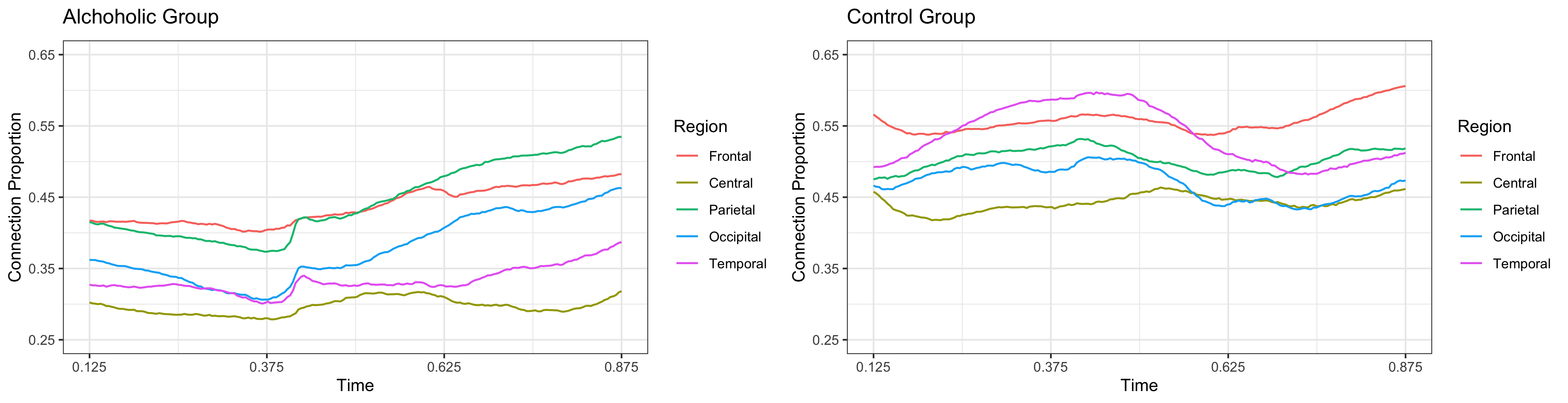
The 64 scalp electrodes can be grouped into five anatomical regions: frontal, central, parietal, occipital, and temporal. Let denote the sets of nodes corresponding to these five anatomical regions, and denote the set of all nodes. We define the connection proportion for region at time as
Figure 4 displays the time-varying connection proportions for each region (averaged across 10 subjects in each group). We have the following observations:
(i) The connection proportions for each region exhibit temporal variations with upward trends, reflecting changes in brain activity in response to the image stimuli presented to the subjects.
(ii) Control subjects demonstrate visibly higher average connection proportions in all brain regions. Similarly, Zhang et al. (1997) reported stronger brain activity in the temporal, occipital, and frontal regions of control subjects, suggesting that long-term alcohol abuse may impair functioning in these regions. While their analysis focused on amplitudes, our results additionally highlight group differences in time-varying correlations.
6.2 Economic Data
The interconnectedness among economic data plays a crucial role in quantifying risks within financial portfolios, as well as systemic and macroeconomic risks. For an introduction, see Acemoglu et al. (2012), Puliga et al. (2014), and Guo et al. (2018), among others. In this section, we infer the time-varying correlation of Daily WRDS World Indices, which are market-capitalization-weighted indices with dividends at daily frequency (for details, see https://wrds-www.wharton.upenn.edu/pages/get-data/world-indices-wrds/).
Specifically, we analyze the weekly averages of the absolute values of the Daily Country Return with Dividends (PORTRET) from June 1, 2006, to June 1, 2022, which can serve as measures of volatility and risk. We denote the weekly average of the absolute value of PORTRET at time for region by . There are time points for regions encompassing France, Germany, the UK, China, Japan, and Hong Kong. Based on these observations, we apply Algorithm 1 and set the target BY level as , equivalently using the adjusted nominal level . For visualization, the time-varying networks are presented in Figure 5. For brevity, the figure displays only the time-varying networks at the first week of June in each year. We restrict the visualization to time points lying away from the boundary and only report the networks for 2011–2018. From the figure, we have the following observations:

(i) The inference results are broadly consistent with known regional/economic linkages. For example, we identify persistent correlations over time between France and Germany, China and Japan, and the UK and Germany, consistent with their strong economic relationships.
(ii) The results also capture substantial temporal variation in correlation. For example, correlations of volatility between Hong Kong and other regions are not statistically significant after the BY adjustment during 2011–2013. This period corresponds to a sharp increase of volatility of the stock market in Hong Kong (Hong Kong Monetary Authority 2012). Additionally, in 2012, the interconnectedness among European countries experienced an obvious shift, driven by the European sovereign debt crisis.
To demonstrate the effectiveness of our method in capturing correlations, we additionally construct a semi-synthetic dataset. We introduce a synthesized country whose weekly average of the absolute value of PORTRET at time is defined as follows. Let be obtained by randomly sampling without replacement from , and represents the data of China. We construct the data of the synthesized country as , where
The resulting semi-synthetic data are denoted by . We then apply Algorithm 1 to estimate the time-varying correlation network. The correlation signal associated with the synthetic country is successfully detected, with an absolute discrepancy of only between the detected time and the true signal time. This implies that our method is capable of detecting time-varying signals accurately and efficiently.
7 Conclusion
This paper studies simultaneous inference for high-dimensional locally stationary time series, with a focus on time-varying correlations. We propose the notion of AuFDR, which is defined as the expectation of -norms of the time-varying FDP, with as sample size . This criterion provides a principled compromise between pointwise FDR control, which fails to ensure reliability over an entire time interval, and the supremum-type criterion, which can be overly sensitive to abrupt local changes in the signal.
Building on this criterion, we develop a general inferential framework for detecting time-varying correlations. The procedure combines robust difference-based estimation with a multiplier bootstrap to generate simultaneously valid -values, followed by a time-varying BY step for AuFDR control under arbitrary dependence. The method is robust to non-Gaussianity, nonlinear dependence, and jumps in means, features common in modern time series data.
Several promising directions remain for future research. First, while this paper focuses on marginal correlations, many applications require inference on conditional dependence structures, such as time-varying partial correlations or graphical models. Extending the AuFDR framework to these settings is an important direction. Second, although the time-varying BY procedure achieves uniform control in our framework, more refined FDR procedures, including adaptive methods, may further improve power while preserving AuFDR guarantees. Third, the AuFDR framework, as a general error-control criterion, may also be useful in other inference problems involving time-varying structures of locally stationary time series.
8 Disclosure Statement
The authors have no conflicts of interest to declare.
9 Data Availability Statement
The brain EEG data is openly available in EEG Database at http://doi.org/10.24432/C5TS3D. The financial data were obtained from the Daily WRDS World Indices database through Wharton Research Data Services (WRDS), University of Pennsylvania (https://wrds-www.wharton.upenn.edu/pages/get-data/world-indices-wrds/). The raw WRDS data are only available from WRDS to users with appropriate institutional subscription and permission.
References
- The network origins of aggregate fluctuations. Econometrica 80 (5), pp. 1977–2016. Cited by: §6.2.
- Complex trend inference for high-dimensional piecewise locally stationary time series. arXiv e-prints, pp. arXiv–2410. Cited by: §4, §\thechapter.B.3, §\thechapter.B.3, §\thechapter.B.3, §\thechapter.B.3, §\thechapter.B.3.
- Uniform variance reduced simultaneous inference of time-varying correlation networks. IEEE Transactions on Information Theory (), pp. 1–1. External Links: Document Cited by: §1.1, §1, §3.1, §3.2, §3.3, §4, §\thechapter.A.1, §\thechapter.A.2, §\thechapter.A.2, §\thechapter.A.3.2, §\thechapter.B.4, §\thechapter.B.5, §\thechapter.B.5.
- A multiple testing approach to the regularisation of large sample correlation matrices. Journal of Econometrics 208 (2), pp. 507–534. Cited by: §1.1.
- Controlling the false discovery rate via knockoffs. The Annals of statistics, pp. 2055–2085. Cited by: §1.1.
- The control of the false discovery rate in multiple testing under dependency. Annals of statistics, pp. 1165–1188. Cited by: §1.1, §1, §3.4, Comment 1.
- Large-scale multiple testing of correlations. Journal of the American Statistical Association 111 (513), pp. 229–240. Cited by: §1.1, §5.3, §\thechapter.C.1, §\thechapter.C.1.
- Optimal difference-based variance estimators in time series: A general framework. The Annals of Statistics 50 (3), pp. 1376 – 1400. External Links: Document Cited by: Remark 4.
- Central limit theorems for high dimensional dependent data. Bernoulli 30 (1), pp. 712–742. Cited by: §1, §4.
- Central limit theorems and bootstrap in high dimensions. The Annals of Probability 45 (4), pp. 2309 – 2352. Cited by: §4, §\thechapter.A.2.
- Estimation and inference of time-varying auto-covariance under complex trend: a difference-based approach. Electronic Journal of Statistics 15 (2), pp. 4264–4294. Cited by: Remark 4.
- Modeling and simulation of financial returns under non-gaussian distributions. Physica A: Statistical Mechanics and its Applications 622, pp. 128886. Cited by: §1.
- Detecting relevant changes in the mean of nonstationary processes—a mass excess approach. The Annals of Statistics 47 (6), pp. 3578–3608. Cited by: Remark 4.
- Confidence surfaces for the mean of locally stationary functional time series. arXiv preprint arXiv:2109.03641. Cited by: §\thechapter.B.1, §\thechapter.B.3.
- Estimation and inference for precision matrices of nonstationary time series. The Annals of Statistics 48 (4), pp. 2455 – 2477. External Links: Document Cited by: §1.
- Correlation and large-scale simultaneous significance testing. Journal of the American Statistical Association 102 (477), pp. 93–103. Cited by: §1.1.
- Conditional calibration for false discovery rate control under dependence. The Annals of Statistics 50 (6), pp. 3091–3118. Cited by: §1.1.
- Development of stock correlation networks using mutual information and financial big data. PloS one 13 (4), pp. e0195941. Cited by: §6.2.
- Asymptotically optimal difference-based estimation of variance in nonparametric regression. Biometrika 77 (3), pp. 521–528. Cited by: Remark 4.
- Economic and financial environment. In Annual Report 2011, pp. 28–39. Note: Published April 30, 2012. Accessed June 30, 2026 External Links: Link Cited by: §6.2.
- Dynamic functional connectivity: promise, issues, and interpretations. Neuroimage 80, pp. 360–378. Cited by: §1.
- Financial modeling under non-gaussian distributions. Springer. Cited by: §1.
- Questions and controversies in the study of time-varying functional connectivity in resting fmri. Network neuroscience 4 (1), pp. 30–69. Cited by: §1, §1.
- A review of two decades of correlations, hierarchies, networks and clustering in financial markets. Progress in information geometry: Theory and applications, pp. 245–274. Cited by: §1.
- Introduction to correlation networks: interdisciplinary approaches beyond thresholding. Physics Reports 1136, pp. 1–39. Cited by: §5.3, §\thechapter.C.1.
- Estimation of heteroscedasticity in regression analysis. The Annals of Statistics, pp. 610–625. Cited by: Remark 4.
- Dynamics of market correlations: taxonomy and portfolio analysis. Physical Review E 68 (5), pp. 056110. Cited by: §1.
- Subsampling. Springer Science & Business Media. Cited by: §3.5.
- Credit default swaps networks and systemic risk. Scientific reports 4 (1), pp. 6822. Cited by: §6.2.
- Autocovariance estimation in regression with a discontinuous signal and m-dependent errors: a difference-based approach. Scandinavian Journal of Statistics, pp. 346–368. Cited by: Remark 4.
- Smoothing noisy data with spline functions. Numerische mathematik 24 (5), pp. 383–393. Cited by: §3.5.
- Nonlinear system theory: another look at dependence. Proceedings of the National Academy of Sciences 102 (40), pp. 14150–14154. Cited by: §4.
- Multiscale jump testing and estimation under complex temporal dynamics. Bernoulli 30 (3), pp. 2372–2398. Cited by: §\thechapter.B.3.
- Convergence of covariance and spectral density estimates for high-dimensional locally stationary processes. The Annals of Statistics 49 (1), pp. 233 – 254. Cited by: §4.
- Gaussian approximation for high dimensional vector under physical dependence. Bernoulli 24 (4A), pp. 2640 – 2675. Cited by: §1, §\thechapter.B.3.
- Electrophysiological evidence of memory impairment in alcoholic patients. Biological Psychiatry 42 (12), pp. 1157–1171. Cited by: §1, §6.1, §6.1, §6.1.
- Simultaneous statistical inference for second order parameters of time series under weak conditions. The Annals of Statistics 52 (5), pp. 2375–2399. Cited by: §1.
- Inference for local autocorrelations in locally stationary models. Journal of Business & Economic Statistics 33 (2), pp. 296–306. Cited by: §4.
SUPPLEMENTARY MATERIAL
Appendix \thechapter.A Technical Appendix
We first provide some additional notations used throughout the Appendix. Let denote convergence in probability. We use to denote and . For an event , let denote its complement. Throughout the Appendix, is the number of hypotheses. Let denote the indicator function. For two positive sequences , write if there exists a constant and such that for all . Write if and . Define as -th order differenced error. We use to denote absolute constants whose values may change from line to line. Constants with a symbolic subscript, such as are used to indicate that their values depend only on the subscript, and may also vary from line to line.
\thechapter.A.1 Proof of Theorem 1
Recall that and further define . Recall the definition of as in (8) and (9). Define the -measurable event
where and is a positive sequence such that and . Recall that is the upper bound of number of abrupt jumps as in Assumption 1(vi). By Lemma 4, we have
| (23) |
Recall the definition of and the definition of norm in (20). Lemma 3 implies
By Lemma 1 and (23), for any ,
| (24) |
Solving , we have . From Assumption 2, and . Under the bandwidth condition , we have . Note that . From Equation (41) of Bai and Wu (2025), we have
| (25) |
By Lemma 1, the above inequality and (24), we have for any ,
In the previous argument we have already set . In this step, set , which gives . We have
Let , . By Lemma 1 and 5, for any ,
Set , we have . By ,
we have . Noticing that since , this gives
In the last line we use as in Assumption 2. Therefore we finish the proof of Theorem 1.
\thechapter.A.2 Proof of Theorem 2
Let denote in one iteration of Algorithm 1. Let , with , where
Here is the set of multiplier Gaussian variables across all dimension and across all time , is the set of multiplier Gaussian variables for the dimension across all time , and is the multiplier Gaussian variable for dimension at time . It follows that . Recall the definition of before Theorem 1. Define
and by substituting in by . Recall the definition of in Theorem 1. Define , . From the proof of Theorem 3 of Bai and Wu (2025), we have
Denote . Using Remark 4.1 of Chernozhukov et al. (2017), we have
| (26) |
Let , , and be an increasing sequence such that . Define the measurable events
| (27) |
By Condition 2, we have . By Lemma 4 and Proposition 2 of Bai and Wu (2025), we have . Similar to Equation (46) and (47) of Bai and Wu (2025), for some sufficiently large constant we have
| (28) | ||||
| (29) |
Recall that we have defined . Pick . From (19), we know that . By (26), (28), (29), Markov inequality and Lemma 1, via some direct but tedious calculation,
Thus we finish the proof of (22).
\thechapter.A.3 Proof of Theorem 3
\thechapter.A.3.1 Proof of (i)
\thechapter.A.3.2 Proof of (ii)
Define as an i.i.d. copy of . Let be a fixed number in . Define . Following the procedure in (38), we have
| (31) |
To further evaluate , we define the following three events: for positive constants , define , and . By Lemma 4, (33), and Proposition 2 of Bai and Wu (2025), we have , which gives . We have the following decomposition:
We first evaluate . Notice that are an i.i.d. copy of , so is independent of . This gives and .
Next we evaluate . We have . Noticing that is -measurable, we have
For any fixed , let , we have , so . So letting , we have .
Define event . By the analysis of , we have , and thus . By (31), we have
In the last line we use the fact that . Since , we have and we finish the proof.
\thechapter.A.4 Proof of Theorem 4
Recall the definition of in (30). Choose such that and ; such a sequence exists because . By the approximation bounds in Theorems 1–2, this choice gives .
Write , so that . Let
be the time region affected by boundary effects or by changes in the true-null set. We have . Therefore,
The first term converges to zero by for some , and .
It remains to bound the second term. For and , we have . Under the time-varying BY procedure, if , then
Hence and . Consequently,
For each , let ; if , the corresponding summand is set to zero. Since the function is nonincreasing, we have
We now bound the expectation of each summand on . By Lemma 6, for every ,
Let for , and denote with in the following summation-by-parts bound. Then
The last inequality follows from the fact that, on , and .
Since , we obtain
By the choice of and the assumption , the last three terms converge to zero. Therefore,
which proves Theorem 4.
Appendix \thechapter.B Additional Technical Proofs
\thechapter.B.1 Lemma 1 and its Proof
Lemma 1.
For any -dimensional random vectors and -dimensional Gaussian random vectors , assume there exists a positive constant such that for . Recall the definition of norm in (20). Then for every and ,
where is a positive constant that only depends on .
\thechapter.B.2 Lemma 2 and its Proof
Lemma 2.
Assume all conditions of Theorem 1. Define
Then we have (i) and their Lipschitz constant are uniformly bounded over . (ii) There exists a positive constant such that . (iii) for some .
Proof. Notice that we have assumed in (i) of Assumption 1 with uniformly bounded Lipschitz constant. Using Cauchy-Schwarz inequality, and their Lipschitz constants are also uniformly bounded. Then (i) comes from the above claim and the fact that are all lower and upper bounded Lipschitz continuous functions with bounded Lipschitz constants as assumed in Assumption 1(iv), and are also bounded Lipschitz continuous functions with bounded Lipschitz constants. We can prove (ii) using similar arguments.
For (iii), using Minkowski inequality, we have
For , using Cauchy-Schwarz inequality we have
Similarly bounds can be obtained for and . Combining the evaluation above, we have . Since are all bounded functions, using Minkowski inequality again we can obtain (iii).
\thechapter.B.3 Lemma 3 and its Proof
Lemma 3.
Proof. Recall the definition of in (9), the definition of in (11), and the definition of before Theorem 1. Define . Let , and . Define the -dependent version of as , and the corresponding -dependent version of are denoted as . Define as the normal vectors with the same covariance structure as . Define and similarly define .
Define if , and . Let , where is a rescaling constant. Define . Let be a continuously differentiable function with finite third order derivatives and . Define and for . Define as a truncation level for , which appears in the intermediate step of the proof of Proposition 6 in Bai et al. (2024) (detailed in the definition of in their paper). For bandwidth , define .
Results in Lemma 2 about corresponds to Condition (A1)-(A3) of Bai et al. (2024). Define . With a very careful investigation of the proof of Proposition 6 and 7 of Bai et al. (2024), we have equation (236) still holds in view of results in Lemma 2 and Assumption 1 with minor modifications, which is, for some small enough but positive constant ,
| (32) |
subject to .
The first difference comes from the term , which results from the fact that in (iii) of Lemma 2 we derive exponential decay of , while in Condition (A3) of Bai et al. (2024) they assume . The second difference is the term . This is due to the tail results of in Lemma 2, which is different from exponential tail condition as imposed in Bai et al. (2024). Recall . By elementary calculation similar to Lemma C.3 in Dette and Wu (2021), noticing that , we have uniformly for ,
| (33) |
Here and are two large enough constants. From Assumption 1(v), using argument in Lemma E.4 of Wu and Zhou (2024), we have for large enough , there exists positive constant such that , with being -th element of . Using argument similar to Lemma A.2 of Zhang and Cheng (2018), noticing that if and is a large enough constant, we have there exist positive constants such that . Using argument of step 5 of Zhang and Cheng (2018) we can derive , where is another constant satisfying . Noticing that has the same covariance structure as , by Proposition 8 of Bai et al. (2024), we have
| (34) |
By (32), (34) and tedious calculation the same as the end of proof of Proposition 7 in Bai et al. (2024), we have
And finally, Lemma 3 comes from the above equation and the fact .
\thechapter.B.4 Lemma 4 and its Proof
Lemma 4.
(i) The difference-based estimator has the following approximation, namely
(ii) The time-varying correlation estimator has the following approximation, namely
\thechapter.B.5 Lemma 5 and its Proof.
Proof. Define event as in (27), and , where is a positive sequence such that and . Recall that in the proof of Theorem 1, we set . By Lemma 4 and , we have . By Proposition 2 of Bai and Wu (2025), we have . Since , from the bandwidth condition in Assumption 2, we have .
In Assumption 1 we assume that , where is a positive absolute constant. So when is large enough, on event , , and
where is a positive absolute constant. This gives
| (35) |
where is an absolute constant, and is defined in an obvious way.
In the following we evaluate . By Cauchy-Schwarz inequality,
| (36) |
On event , if is large enough, there exists a constant satisfying . This gives there exist another positive constant , such that . So using Proposition 2 of Bai and Wu (2025), we have
| (37) |
For the evaluation of , recall the definition of as in (8), and . From Lemma 2(i), we have . Using (23), (\thechapter.A.1) and Minkowski inequality, we have
The last line comes from the fact that from bandwidth conditions in Assumption 2. So we have . By (\thechapter.B.5) and (37) we have . Recall that we have taken . By the bound of , , and (35) we finish the proof of Lemma 5.
\thechapter.B.6 Lemma 6 and its Proof
Recall that denote the set of time points at which the null hypothesis is true. Its interior region, after removing a boundary band of width , is defined by . Recall the definition of in (30).
Lemma 6.
Assume all conditions in Theorem 3 hold. Then we have
Proof. Recall the definition of in Algorithm 1. Let be an identically distributed and independent copy of centered version of , which is . For we have the following decomposition . The -value satisfies . Given , the terms in the summation are independent. Therefore,
| (38) |
Since has the same distribution as , by Lemma 7,
for . So by (38),
\thechapter.B.7 Lemma 7 and its Proof
Lemma 7.
Assume are independent and identically distributed random variables with distribution function . Then we have for all .
Proof. Let for . Then we have
For any , from the definition of , we have . This gives , and thus .
Appendix \thechapter.C Additional Simulations
\thechapter.C.1 Baseline Comparison
We compare our method to the moving-window approach (denoted as MW) described in Section 3.9 of Masuda et al. (2025). This method selects a window length and, at time , computes sample correlations using data from the time interval . Correlation is detected at time if the sample correlation exceeds a chosen threshold . As pointed out in Masuda et al. (2025), there is no consensus on an optimal method for selecting . For brevity, we report this moving-window comparison only for Cases 1–2 with Gaussian innovations. The results in Table 5 show that, depending on , the method can either produce an excessively high AuFDP or be overly conservative.
| Average FNP | |||||
|---|---|---|---|---|---|
| 6 | 600 | 0.300 | 0.005 | 0.000 | 0.062 |
| 900 | 0.264 | 0.000 | 0.000 | 0.047 | |
| 1500 | 0.221 | 0.000 | 0.000 | 0.026 | |
| 9 | 600 | 0.414 | 0.017 | 0.000 | 0.061 |
| 900 | 0.368 | 0.000 | 0.000 | 0.045 | |
| 1500 | 0.291 | 0.000 | 0.000 | 0.027 | |
We further compare Algorithm 1 with the multiple-testing procedure of Cai and Liu (2016) (referred to as MT). The original MT procedure was developed for zero-mean stationary time series. To make it applicable in the present locally stationary setting, we implement a moving-window version: for a given bandwidth , the MT procedure is applied at time using only observations with . To ensure a fair comparison, we set the mean functions to zero when applying both the MT method and Algorithm 1. For brevity, we also report the MT comparison only for Cases 1–2 with Gaussian innovations.
The results, summarized in Table 6, reveal several key limitations of the MT method compared to Algorithm 1. First, the MT method exhibits a thresholding behavior (see Remark 1 of Cai and Liu (2016)) and fails to respond to small nominal levels, yielding identical and values across and . Furthermore, its tends to rise with and exceeds the theoretical upper bounds established in our analysis. In contrast, our proposed method maintains stable AuFDP control across all tested levels and sample sizes while demonstrating a consistent reduction in AuFNP as grows.
| Method | Average FNP | |||||
|---|---|---|---|---|---|---|
| Alg 1 | 6 | 600 | 0.040 | 0.058 | 0.084 | 0.062 |
| 900 | 0.025 | 0.041 | 0.031 | 0.022 | ||
| 1500 | 0.030 | 0.044 | 0.005 | 0.003 | ||
| 9 | 600 | 0.046 | 0.060 | 0.107 | 0.081 | |
| 900 | 0.043 | 0.056 | 0.053 | 0.036 | ||
| 1500 | 0.043 | 0.059 | 0.008 | 0.004 | ||
| MT | 6 | 600 | 0.088 | 0.088 | 0.006 | 0.006 |
| 900 | 0.088 | 0.088 | 0.000 | 0.000 | ||
| 1500 | 0.100 | 0.100 | 0.000 | 0.000 | ||
| 9 | 600 | 0.082 | 0.082 | 0.011 | 0.011 | |
| 900 | 0.082 | 0.082 | 0.001 | 0.001 | ||
| 1500 | 0.086 | 0.086 | 0.000 | 0.000 | ||
\thechapter.C.2 Sensitivity Analysis
In this section, we assess the robustness of Algorithm 1 with respect to the choice of tuning parameters. For brevity, we report sensitivity results only for Cases 1–2 under Gaussian innovations.
First, we consider perturbations of to the bandwidths selected via the data-driven procedure described in Section 3.5. Second, we evaluate the sensitivity to the lag parameter . Our main results use with , while the sensitivity to is assessed by considering perturbations, namely and .
Tables 7 and 8 report the sensitivity results, showing that Algorithm 1 is robust to perturbations of both the bandwidth and the lag parameter.
| Perturbation | Average FNP | |||||
|---|---|---|---|---|---|---|
| -0.1 | 6 | 600 | 0.024 | 0.036 | 0.173 | 0.138 |
| 900 | 0.015 | 0.021 | 0.091 | 0.064 | ||
| 1500 | 0.018 | 0.025 | 0.020 | 0.012 | ||
| 9 | 600 | 0.027 | 0.036 | 0.207 | 0.170 | |
| 900 | 0.021 | 0.033 | 0.128 | 0.094 | ||
| 1500 | 0.023 | 0.035 | 0.034 | 0.020 | ||
| 0.0 | 6 | 600 | 0.037 | 0.057 | 0.087 | 0.066 |
| 900 | 0.024 | 0.043 | 0.032 | 0.024 | ||
| 1500 | 0.031 | 0.042 | 0.005 | 0.003 | ||
| 9 | 600 | 0.045 | 0.057 | 0.110 | 0.085 | |
| 900 | 0.041 | 0.056 | 0.055 | 0.037 | ||
| 1500 | 0.043 | 0.060 | 0.008 | 0.004 | ||
| 0.1 | 6 | 600 | 0.057 | 0.077 | 0.041 | 0.031 |
| 900 | 0.044 | 0.065 | 0.014 | 0.009 | ||
| 1500 | 0.046 | 0.062 | 0.002 | 0.001 | ||
| 9 | 600 | 0.067 | 0.083 | 0.053 | 0.037 | |
| 900 | 0.064 | 0.080 | 0.021 | 0.013 | ||
| 1500 | 0.062 | 0.081 | 0.002 | 0.001 | ||
| Average FNP | ||||||
|---|---|---|---|---|---|---|
| 0.8 | 6 | 600 | 0.038 | 0.055 | 0.093 | 0.071 |
| 900 | 0.033 | 0.046 | 0.037 | 0.026 | ||
| 1500 | 0.023 | 0.034 | 0.008 | 0.004 | ||
| 9 | 600 | 0.053 | 0.067 | 0.113 | 0.088 | |
| 900 | 0.036 | 0.051 | 0.053 | 0.036 | ||
| 1500 | 0.034 | 0.046 | 0.015 | 0.009 | ||
| 1.0 | 6 | 600 | 0.037 | 0.057 | 0.087 | 0.066 |
| 900 | 0.024 | 0.043 | 0.032 | 0.024 | ||
| 1500 | 0.031 | 0.042 | 0.005 | 0.003 | ||
| 9 | 600 | 0.045 | 0.057 | 0.110 | 0.085 | |
| 900 | 0.041 | 0.056 | 0.055 | 0.037 | ||
| 1500 | 0.043 | 0.060 | 0.008 | 0.004 | ||
| 1.2 | 6 | 600 | 0.046 | 0.060 | 0.087 | 0.066 |
| 900 | 0.027 | 0.043 | 0.036 | 0.026 | ||
| 1500 | 0.028 | 0.039 | 0.007 | 0.005 | ||
| 9 | 600 | 0.054 | 0.073 | 0.110 | 0.086 | |
| 900 | 0.044 | 0.062 | 0.057 | 0.040 | ||
| 1500 | 0.048 | 0.058 | 0.013 | 0.008 | ||
Comment 1 (Connection between Benjamini–Hochberg (BH) and BY procedure).
Similar to the BY procedure, the Benjamini–Hochberg (BH) procedure is also a classical FDR control procedure: after ordering the -values, it determines the rejection threshold by choosing an integer such that
and rejects all null hypotheses whose -values . It controls the FDR under independence or positive regression dependence on a subset (PRDS) (Benjamini and Yekutieli 2001). In our setting, these conditions are often violated because the time-varying -values share common bootstrap samples and inherit complex cross-sectional dependence across and temporal dependence across . We therefore use the BY procedure, which lowers the nominal level in the BH procedure by the harmonic factor . This adjustment allows us to work without dependence restrictions and yields the asymptotic AuFDR bound in Theorem 4.