跳到论文正文
W Papers独立论文阅读器 arXiv:2512.10366 论文正文 计算阅读时间 · 0%
引用这篇论文根据当前论文元数据生成,正式投稿前建议核对。


License: arXiv.org perpetual non-exclusive license
arXiv:2512.10366v2 [math.OC] 13 May 2026

Primal-dual splitting for structured composite monotone inclusions with or without cocoercivity

Minh N. Dao,   Hung M. Phan,   Matthew K. Tam,  and  Thang D. Truong School of Science, RMIT University, Melbourne, VIC 3000, Australia. E-mail: minh.dao@rmit.edu.au.Department of Mathematics and Statistics, Kennedy College of Sciences, University of Massachusetts Lowell, Lowell, MA 01854, USA. E-mail: hung_phan@uml.edu.School of Mathematics and Statistics, The University of Melbourne, Parkville, VIC 3010, Australia. E-mail: matthew.tam@unimelb.edu.au.School of Science, RMIT University, Melbourne, VIC 3000, Australia. E-mail: thang.tdk64@gmail.com.
(May 13, 2026)
Abstract

In this paper, we propose a primal-dual splitting algorithm for a broad class of structured composite monotone inclusions that involve finitely many set-valued operators, compositions of set-valued operators with bounded linear operators, and single-valued operators possibly without cocoercivity. The proposed algorithm is not only a unification for several contemporary algorithms but also a blueprint to generate new algorithms with graph-based structures using a single transparent convergence analysis. Our approach reduces dimensionality compared with the standard product space technique, which typically reformulates the original problem as the sum of two maximally monotone operators in order to apply splitting methods. It accommodates different cocoercive or Lipschitz constants as well as different resolvent parameters, and yields a larger allowable stepsize range than recent methods. We demonstrate the practicality of the approach by a numerical experiment on cancer detection using the decentralized fused LASSO problem.

Keywords: Distributed optimization, composite monotone inclusions, splitting algorithms, primal-dual algorithms, fused LASSO problem.

Mathematics Subject Classification (MSC 2020): 47H05, 47H10, 65K10, 90C30.

1 Introduction

Many interesting problems such as composite optimization problems, structured saddle-point problems, and variational inequalities can be formulated as monotone inclusion problems [17, 28, 29]. Among the most widely used methods for solving such problems are splitting algorithms, in which computations are performed separately on each operator instead of their sums, see, e.g., [8, 21, 23, 25, 31, 35]. When an optimization problem involves compositions of set-valued operators with bounded linear operators, common mathematical tools such as resolvents can be computed for such compositions, however, it is generally very difficult, thus, not desirable. Instead, primal-dual splitting algorithms [3, 12, 15, 19, 36] are usually used to process the set-valued operators separately using backward steps via their resolvents, while the bounded linear operators are evaluated directly using forward steps on their own or on their adjoints. Considering the primal inclusion and the dual inclusion simultaneously provides us a better understanding of the problem.

Let ℋ\mathcal{H} and (𝒢k)1≤k≤r(\mathcal{G}_{k})_{1\leq k\leq r} be real Hilbert spaces. We consider the primal inclusion

find ​x∈ℋ​ such that ​0∈∑i=1nAi​x+∑k=1rLk∗​Bk​Lk​x+∑j=1pCj​x,\displaystyle\text{find }x\in\mathcal{H}\text{ such that }0\in\sum_{i=1}^{n}A_{i}x+\sum_{k=1}^{r}L_{k}^{*}B_{k}L_{k}x+\sum_{j=1}^{p}C_{j}x, (1)

where, for each i∈{1,…,n}i\in\{1,\dots,n\}, Ai:ℋ⇉ℋA_{i}\colon\mathcal{H}\rightrightarrows\mathcal{H} is a maximally monotone operator, for each k∈{1,…,r}k\in\{1,\dots,r\}, Bk:𝒢k⇉𝒢kB_{k}\colon\mathcal{G}_{k}\rightrightarrows\mathcal{G}_{k} is a maximally monotone operator and Lk:ℋ→𝒢kL_{k}\colon\mathcal{H}\rightarrow\mathcal{G}_{k} is a bounded linear operator with adjoint operator Lk∗L_{k}^{*}, and for each j∈{1,…,p}j\in\{1,\dots,p\}, Cj:ℋ→ℋC_{j}\colon\mathcal{H}\to\mathcal{H} is either a cocoercive operator, or a monotone and Lipschitz continuous operator. Problem (1) arises in a wide range of applications, including location problems [10], image reconstruction [15], and signal processing [17]. The associated dual inclusion in the sense of Attouch–Théra [6] is

find ​(s1,…,sr)∈∏k=1r𝒢k​ such that 0∈−Lk​(∑i=1nAi+∑j=1pCj)−1​(−∑k=1rLk∗​sk)+Bk−1​sk,k∈{1,…,r}.\displaystyle\begin{aligned} &\text{find }(s_{1},\dots,s_{r})\in\prod_{k=1}^{r}\mathcal{G}_{k}\text{~such that~}\\ &0\in-L_{k}\left(\sum_{i=1}^{n}A_{i}+\sum_{j=1}^{p}C_{j}\right)^{-1}\left(-\sum_{k=1}^{r}L_{k}^{*}s_{k}\right)+B_{k}^{-1}s_{k},\quad k\in\{1,\dots,r\}.\end{aligned} (2)

When n≠0n\neq 0, r=0r=0, and p=0p=0, problem (1) reduces to finding a zero in the sum of finitely many maximally monotone operators that are potentially set-valued. The most well-known algorithm for the classical case n=2n=2 is the Douglas–Rachford algorithm [21]. Recently, a splitting algorithm was proposed for n=3n=3 by Ryu [31], while a different resolvent splitting for the general case n≥2n\geq 2 was introduced by Malitsky and Tam [25]. The latter work was then extended into a framework [32] that covers these algorithms. In the setting when n≠0n\neq 0, r=0r=0, and p≠0p\neq 0, the problems involve not only maximally monotone operators but also single-valued operator which can be used directly by forward evaluations. When n=1n=1 and p=1p=1, the forward-backward algorithm [23] is typically used when CC is cocoercive, while the forward-backward-forward algorithm [35] and the forward-reflected-backward algorithm [24] are commonly applied when CC is monotone and Lipschitz continuous. Moreover, the authors of [5] developed a distributed forward-backward algorithm for the case where n≥2n\geq 2, p=n−1p=n-1, and each CjC_{j} is cocoercive, as well as a second algorithm for n≥3n\geq 3, p=n−2p=n-2, and each CjC_{j} monotone and Lipschitz continuous. Recently, the forward-backward algorithms devised by graphs in [4] and a class of algorithms in [2] effectively characterized methods that use only individual resolvent evaluations and direct evaluations of cocoercive operators, while a general approach to distributed operator splitting [20] addresses the situations where the single-valued operators may not be cocoercive.

In the setting when r≠0r\neq 0, there are many primal-dual algorithms are proposed, but only for some special cases of problem (1). For example, in the case n=1n=1, r=1r=1, and p=0p=0, popular algorithms include the Chambolle–Pock algorithm [15] and an algorithm proposed by Briceño-Arias and Combettes [12]. When n=0n=0, r=1r=1, and p=1p=1, one can use primal-dual fixed-point algorithm based on the proximity operator (PDFP2O) or proximal alternating predictor-corrector (PAPC) [16, 22]. For the case where n=1n=1, r=1r=1, and p=1p=1, or when a Lipschitz and a cocoercive operator are treated simultaneously, we refer interested readers to [18, 19, 30, 36]. When r≥2r\geq 2, one can adapt some of the above algorithms and use product space reformulations, even though it may not utilize different structures of algorithm design. Recently, Aragón-Artacho et al. [3] studied the case with n≥2n\geq 2, r=1r=1, and p=0p=0 in the reduced dimension n−1n-1. Then, to incorporate multiple bounded linear operators with r≥2r\geq 2, the proposed algorithm, however, still relies on a product space reformulation.

Most of the aforementioned algorithms reformulate the original problem as the sum of a maximally monotone operator and a skew-symmetric or cocoercive operator, then apply the forward-backward [19, 36] or forward-backward-forward approach [12, 18]. In this work, we introduce a primal-dual splitting algorithm for structured composite monotone inclusions that unifies many well-known algorithms in the literature through a single transparent convergence analysis. Our algorithm provides a different perspective using reduced dimension n−1+rn-1+r compared to dimension n+rn+r using product space reformulations which potentially contribute to the theory and applications of primal-dual algorithms. Furthermore, we directly handle the linear operators L1,…,LrL_{1},\dots,L_{r}, rather than through a product space reformulation, which allows us to generate alternative designs with potentially significantly larger stepsizes compared to those in [3, Corollary 1]. Therefore, this approach facilitates distributed computation without central coordination which helps prevent bottlenecks that arise from centralized coordination in practice. In addition, different cocoercive or Lipschitz constants, as well as resolvent parameters are also allowed for distributed implementation without requiring the knowledge of a global cocoercive or Lipschitz constant.

In this work, our main contributions are as follows.

  1. (i)

    We develop a primal-dual algorithm for structured composite monotone inclusions involving finitely many set-valued operators, composition of set-valued operators with bounded linear operators, and single-valued operators that may not be cocoercive. Our algorithm does not rely on reformulating the original problem as the sum of a maximally monotone operator and a skew-symmetric or cocoercive operator using product space reformulations but rather directly exploit the problem structure to derive different algorithm designs, offer possibly larger stepsize ranges with explicit formulas. For our convergence analysis, we introduce the concept of quasicomonotonicity in Definition 2.1(ii) and its natural connection to quasiaveragedness [20, Definition 2.1].

  2. (ii)

    The proposed algorithm not only unifies several contemporary methods but also provides a general framework for constructing new graph-based algorithms within a single unified convergence analysis. Notably, our analysis enables the derivation of broader admissible stepsize ranges under weaker assumptions on the coefficient matrices compared with recent methods [2, 3, 20]. Moreover, the algorithm also allows different cocoercive or Lipschitz constants as well as different resolvent parameters suitable for distributed implementation, thereby improving upon certain existing methods. Finally, we explore various choices of the coefficient matrices of the algorithm and examine the effect of stepsizes on the algorithm’s performance in a numerical experiment on cancer detection using the decentralized fused LASSO problem.

The remainder of this paper is structured as follows. In Section 2, we introduce some notations and background materials on set-valued, single-valued operators, Kronecker product, and solution sets of the primal and dual problem. In Section 3, we present our primal-dual splitting algorithm in Algorithm 1 with main convergence results in Theorem 3.11. We discuss the relation to existing algorithms and new algorithms in Section 4. Section 5 provides a numerical experiment on the decentralized fused LASSO problem for cancer detection, examining the performance of the algorithm under different settings of the coefficient matrices and parameters.

2 Preliminaries

In this paper, the sets of nonnegative integers and real numbers are denoted by ℕ\mathbb{N} and ℝ\mathbb{R}, respectively. We assume that ℋ\mathcal{H} and (𝒢k)1≤k≤r(\mathcal{G}_{k})_{1\leq k\leq r} are real Hilbert spaces equipped with their respective inner product ⟨⋅,⋅⟩\left\langle\cdot,\cdot\right\rangle and induced norm ∥⋅∥\|\cdot\|. Unless otherwise stated, we use the standard inner product in the product space ℋn\mathcal{H}^{n}, i.e., for 𝐱=(x1,…,xn)∈ℋn{\mathbf{x}}=(x_{1},\ldots,x_{n})\in\mathcal{H}^{n} and 𝐱¯=(x¯1,…,x¯n)∈ℋn\bar{\mathbf{x}}=(\bar{x}_{1},\ldots,\bar{x}_{n})\in\mathcal{H}^{n},

⟨𝐱,𝐱¯⟩=∑i=1n⟨xi,x¯i⟩.\displaystyle\left\langle{\mathbf{x}},\bar{\mathbf{x}}\right\rangle=\sum_{i=1}^{n}\left\langle x_{i},\bar{x}_{i}\right\rangle.

With this inner product, we say that a linear operator Ψ:ℋn→ℋn\Psi:\mathcal{H}^{n}\to\mathcal{H}^{n} is positive semidefinite, denoted by Ψ⪰0\Psi\succeq 0 if, for all 𝐱∈ℋn{\mathbf{x}}\in\mathcal{H}^{n}, ⟨𝐱,Ψ​𝐱⟩≥0\left\langle{\mathbf{x}},\Psi{\mathbf{x}}\right\rangle\geq 0. Strong and weak convergence of sequences are denoted by →\rightarrow and ⇀\rightharpoonup, respectively.

For an operator AA on ℋ\mathcal{H}, we write A:ℋ⇉ℋA\colon\mathcal{H}\rightrightarrows\mathcal{H} when AA is set-valued, and A:ℋ→ℋA\colon\mathcal{H}\to\mathcal{H} when AA is single-valued. For such an operator AA, the domain, graph, fixed-point set, and zero set are defined by dom⁡A:={x∈ℋ:A​x≠∅}\operatorname{dom}A:=\{x\in\mathcal{H}:Ax\neq\varnothing\}, gra⁡A:={(x,u)∈ℋ×ℋ:u∈A​x}\operatorname{gra}A:=\{(x,u)\in\mathcal{H}\times\mathcal{H}:u\in Ax\}, Fix⁡A:={x∈ℋ:x∈A​x}\operatorname{Fix}A:=\{x\in\mathcal{H}:x\in Ax\}, and zer⁡A:={x∈ℋ:0∈A​x}\operatorname{zer}A:=\{x\in\mathcal{H}:0\in Ax\}, respectively. The resolvent of AA is defined by JA:=(Id+A)−1J_{A}:=(\operatorname{Id}+A)^{-1}, where Id\operatorname{Id} denotes the identity operator. We say that AA is monotone if, for all (x,u),(y,v)∈gra⁡A(x,u),(y,v)\in\operatorname{gra}A,

⟨x−y,u−v⟩≥0\displaystyle\left\langle x-y,u-v\right\rangle\geq 0

and maximally monotone if it is monotone and there exists no monotone operator whose graph properly contains gra⁡A\operatorname{gra}A.

An operator C:ℋ→ℋC\colon\mathcal{H}\to\mathcal{H} is ℓ\ell-Lipschitz continuous for ℓ∈[0,+∞)\ell\in[0,+\infty) if, for all x,y∈ℋx,y\in\mathcal{H}, ‖C​x−C​y‖≤ℓ​‖x−y‖\|Cx-Cy\|\leq\ell\|x-y\| and 1ℓ\frac{1}{\ell}-cocoercive for ℓ∈(0,+∞)\ell\in(0,+\infty) if, for all x,y∈ℋx,y\in\mathcal{H}, ⟨C​x−C​y,x−y⟩≥1ℓ​‖C​x−C​y‖2\left\langle Cx-Cy,x-y\right\rangle\geq\frac{1}{\ell}\|Cx-Cy\|^{2}. By the Cauchy–Schwarz inequality, every 1ℓ\frac{1}{\ell}-cocoercive operator is monotone and ℓ\ell-Lipschitz continuous, which, in turn, means that it is also maximally monotone [8, Corollary 20.28].

For our convergence analysis, we will recall several related concepts.

Definition 2.1.

We say that

  1. (i)

    Γ:ℋ→ℋ\Gamma:\mathcal{H}\to\mathcal{H} is α\alpha-comonotone [9, Definition 2.4] with α∈ℝ\alpha\in\mathbb{R} if, for all x,y∈ℋx,y\in\mathcal{H},

    ⟨Γ​x−Γ​y,x−y⟩≥α​‖Γ​x−Γ​y‖2.\displaystyle\left\langle\Gamma x-\Gamma y,x-y\right\rangle\geq\alpha\|\Gamma x-\Gamma y\|^{2}.
  2. (ii)

    Γ\Gamma is α\alpha-quasicomonotone (with respect to the set zer⁡Γ\operatorname{zer}\Gamma) if, for all x∈ℋx\in\mathcal{H} and y∈zer⁡Γy\in\operatorname{zer}\Gamma,

    ⟨Γ​x,x−y⟩≥α​‖Γ​x‖2.\displaystyle\left\langle\Gamma x,x-y\right\rangle\geq\alpha\|\Gamma x\|^{2}.

    Unless stated otherwise, we will simply say Γ\Gamma is α\alpha-quasicomonotone and drop the reference set zer⁡Γ\operatorname{zer}\Gamma.

  3. (iii)

    T:ℋ→ℋT\colon\mathcal{H}\to\mathcal{H} is conically ρ\rho-averaged [7, Definition 2.1] with ρ∈(0,+∞)\rho\in(0,+\infty) if, for all x,y∈ℋx,y\in\mathcal{H},

    ‖T​x−T​y‖2+1−ρρ​‖(Id−T)​x−(Id−T)​y‖2≤‖x−y‖2,\displaystyle\|Tx-Ty\|^{2}+\frac{1-\rho}{\rho}\|(\operatorname{Id}-T)x-(\operatorname{Id}-T)y\|^{2}\leq\|x-y\|^{2},
  4. (iv)

    TT is conically ρ\rho-quasiaveraged (with respect to the set Fix⁡T\operatorname{Fix}T) [20, Definition 2.1] if, ρ∈(0,+∞)\rho\in(0,+\infty) and for all x∈ℋx\in\mathcal{H} and all y∈Fix⁡Ty\in\operatorname{Fix}T,

    ‖T​x−y‖2+1−ρρ​‖(Id−T)​x‖2≤‖x−y‖2.\displaystyle\|Tx-y\|^{2}+\frac{1-\rho}{\rho}\|(\operatorname{Id}-T)x\|^{2}\leq\|x-y\|^{2}.

    Unless stated otherwise, we will simply say TT is conically ρ\rho-quasiaveraged and drop the reference set Fix⁡T\operatorname{Fix}T.

Clearly, every conically ρ\rho-averaged operator is conically ρ\rho-quasiaveraged. It is known from [7, Proposition 3.3] that, for α,θ∈(0,+∞)\alpha,\theta\in(0,+\infty), Γ\Gamma is α\alpha-comonotone if and only if Id−θ​Γ\operatorname{Id}-\theta\Gamma is conically θ2​α\frac{\theta}{2\alpha}-averaged. Naturally, we will derive a similar connection between conical quasiaveragedness and quasicomonotonicity.

Proposition 2.2.

Let Γ:ℋ→ℋ\Gamma\colon\mathcal{H}\to\mathcal{H} and α,θ∈(0,+∞)\alpha,\theta\in(0,+\infty). Then Γ\Gamma is α\alpha-quasicomonotone if and only if T:=Id−θ​ΓT:=\operatorname{Id}-\theta\Gamma is conically θ2​α\frac{\theta}{2\alpha}-quasiaveraged.

Take x¯∈Fix⁡T=zer⁡Γ\bar{x}\in\operatorname{Fix}T=\operatorname{zer}\Gamma and take any x∈ℋx\in\mathcal{H}. Then TT is conically θ2​α\frac{\theta}{2\alpha}-quasiaveraged

⇔\displaystyle\iff\quad ‖T​x−x¯‖2+1−θ/(2​α)θ/(2​α)​‖(Id−T)​x‖2\displaystyle\|Tx-\bar{x}\|^{2}+\frac{1-\theta/(2\alpha)}{\theta/(2\alpha)}\|(\operatorname{Id}-T)x\|^{2} ≤‖x−x¯‖2\displaystyle\leq\|x-\bar{x}\|^{2}
⇔\displaystyle\iff ‖x−θ​Γ​x−x¯‖2+2​α−θθ​‖θ​Γ​x‖2\displaystyle\|x-\theta\Gamma x-\bar{x}\|^{2}+\frac{2\alpha-\theta}{\theta}\|\theta\Gamma x\|^{2} ≤‖x−x¯‖2\displaystyle\leq\|x-\bar{x}\|^{2}
⇔\displaystyle\iff −2​⟨θ​Γ​x,x−x¯⟩+‖θ​Γ​x‖2+(2​α−θ)​θ​‖Γ​x‖2\displaystyle-2\left\langle\theta\Gamma x,x-\bar{x}\right\rangle+\|\theta\Gamma x\|^{2}+(2\alpha-\theta)\theta\|\Gamma x\|^{2} ≤0\displaystyle\leq 0
⇔\displaystyle\iff α​‖Γ​x‖2\displaystyle\alpha\|\Gamma x\|^{2} ≤⟨Γ​x,x−x¯⟩,\displaystyle\leq\left\langle\Gamma x,x-\bar{x}\right\rangle,

which means Γ\Gamma is α\alpha-quasicomonotone. ∎

2.1 Kronecker product, the vector 𝟙{\mathbbm{1}}, and the diagonal set Σ\Sigma

For a matrix MM, we denote its range and kernel by ran⁡M\operatorname{ran}M and ker⁡M\ker M, respectively, its transpose by M⊤M^{\top}, and its pseudo-inverse by M†M^{\dagger}. For a positive diagonal matrix E=diag⁡(η1,…,ηn){E}=\operatorname{diag}(\eta_{1},\ldots,\eta_{n}) where ηi∈(0,+∞)\eta_{i}\in(0,+\infty), we denote its square root matrix by E=diag⁡(η1,…,ηn)\sqrt{{E}}=\operatorname{diag}(\sqrt{\eta_{1}},\ldots,\sqrt{\eta_{n}}). Clearly, E​E=E\sqrt{{E}}\sqrt{{E}}={E}.

In an abuse of notation, we identify matrices M=(Mi​j)∈ℝn×mM=(M_{ij})\in\mathbb{R}^{n\times m} with the Kronecker product (M⊗Id):ℋm→ℋn(M\otimes\operatorname{Id})\colon\mathcal{H}^{m}\to\mathcal{H}^{n}. Therefore, for any 𝐳=(z1,…,zm)∈ℋm{\mathbf{z}}=(z_{1},\dots,z_{m})\in\mathcal{H}^{m}, we have

M​𝐳:=(M⊗Id)​𝐳=(∑j=1mM1​j​zj,∑j=1mM2​j​zj,…,∑j=1mMn​j​zj)∈ℋn.M{\mathbf{z}}:=(M\otimes\operatorname{Id}){\mathbf{z}}=\left(\sum_{j=1}^{m}M_{1j}z_{j},\sum_{j=1}^{m}M_{2j}z_{j},\ldots,\sum_{j=1}^{m}M_{nj}z_{j}\right)\in\mathcal{H}^{n}.

Let A1,…,An:ℋ⇉ℋA_{1},\dots,A_{n}\colon\mathcal{H}\rightrightarrows\mathcal{H} be maximally monotone operators. Given 𝐱=(x1,…,xn)∈ℋn{\mathbf{x}}=(x_{1},\dots,x_{n})\in\mathcal{H}^{n}, we define the operator 𝑨:ℋn⇉ℋn{\boldsymbol{A}}\colon\mathcal{H}^{n}\rightrightarrows\mathcal{H}^{n} by 𝑨​𝐱:=A1​x1×⋯×An​xn{\boldsymbol{A}}{\mathbf{x}}:=A_{1}x_{1}\times\dots\times A_{n}x_{n}. It follows that 𝑨{\boldsymbol{A}} is also a maximally monotone operator. As a consequence, its resolvent J𝑨:ℋn→ℋnJ_{{\boldsymbol{A}}}\colon\mathcal{H}^{n}\rightarrow\mathcal{H}^{n} is given by J𝑨=(JA1,…,JAn)J_{{\boldsymbol{A}}}=(J_{A_{1}},\dots,J_{A_{n}}). Note that we can write 𝑨{\boldsymbol{A}} and J𝑨J_{{\boldsymbol{A}}} as diagonal operators

𝑨=[A10⋱0An]​ and ​J𝑨=[JA10⋱0JAn].\displaystyle{\boldsymbol{A}}=\begin{bmatrix}A_{1}&&0\\ &\ddots&\\ 0&&A_{n}\end{bmatrix}\text{ and }J_{\boldsymbol{A}}=\begin{bmatrix}J_{A_{1}}&&0\\ &\ddots&\\ 0&&J_{A_{n}}\end{bmatrix}.

Similarly, we define the diagonal operators

𝑩:=[B10⋱0Br],𝑳:=[L10⋱0Lr],𝑪:=[C10⋱0Cp],\displaystyle{\boldsymbol{B}}:=\begin{bmatrix}B_{1}&&0\\ &\ddots&\\ 0&&B_{r}\end{bmatrix},\ {\boldsymbol{L}}:=\begin{bmatrix}L_{1}&&0\\ &\ddots&\\ 0&&L_{r}\end{bmatrix},\ {\boldsymbol{C}}:=\begin{bmatrix}C_{1}&&0\\ &\ddots&\\ 0&&C_{p}\end{bmatrix},

where the operators BkB_{k}, LkL_{k}, and CjC_{j} are from the setup of problem (1).

We denote 𝟙n=(1,…,1)∈ℝn{\mathbbm{1}}_{n}=(1,\ldots,1)\in\mathbb{R}^{n}. When the context is clear, we will drop the subscript and simply write 𝟙{\mathbbm{1}}, for example, if M∈ℝm×nM\in\mathbb{R}^{m\times n}, then 𝟙⊤​M​𝟙=(𝟙m)⊤​M​(𝟙n){\mathbbm{1}}^{\top}M{\mathbbm{1}}=({\mathbbm{1}}_{m})^{\top}M({\mathbbm{1}}_{n}). Using this notation, we can define the diagonal set

Σn:={𝐱=(x,…,x)∈ℋn}={(𝟙n)​x:x∈ℋ},\displaystyle\Sigma_{n}:=\{{\mathbf{x}}=(x,\dots,x)\in\mathcal{H}^{n}\}=\{({\mathbbm{1}}_{n})x\ :\ x\in\mathcal{H}\},

and thus its the orthogonal set is Σn⊥={𝐱^∈ℋn: 1⊤​𝐱^=0}\Sigma_{n}^{\bot}=\{\hat{{\mathbf{x}}}\in\mathcal{H}^{n}\,:\,{\mathbbm{1}}^{\top}\hat{{\mathbf{x}}}=0\}. Again, we will drop the subscript and denote 𝟙​x{\mathbbm{1}}x when the dimension is clear. In particular, for x∈ℋx\in\mathcal{H}, 𝑨​(𝟙​x)=(A1​x,…,An​x){\boldsymbol{A}}({\mathbbm{1}}x)=(A_{1}x,\ldots,A_{n}x), 𝑳​(𝟙​x)=(L1​x,…,Lr​x){\boldsymbol{L}}({\mathbbm{1}}x)=(L_{1}x,\ldots,L_{r}x), and 𝑪​(𝟙​x)=(C1​x,…,Cp​x){\boldsymbol{C}}({\mathbbm{1}}x)=(C_{1}x,\ldots,C_{p}x).

2.2 Solution sets of the primal and dual problems

The sets of solutions to (1) and (2) are denoted by 𝒫\mathcal{P} and 𝒟\mathcal{D}, respectively. Let 𝒁{\boldsymbol{Z}} be a subset of 𝒫×𝒟\mathcal{P}\times\mathcal{D} such that

𝒁\displaystyle{\boldsymbol{Z}} ={(x,𝐬)∈ℋ×∏k=1r𝒢k:𝐬=(s1,…,sr)∈∏k=1rBk​Lk​x​ and ​0∈∑i=1nAi​x+∑k=1rLk∗​sk+∑j=1pCj​x}\displaystyle=\Bigg\{(x,{\mathbf{s}})\in\mathcal{H}\times\prod_{k=1}^{r}\mathcal{G}_{k}:\ {\mathbf{s}}=(s_{1},\dots,s_{r})\in\prod_{k=1}^{r}B_{k}L_{k}x\text{~and~}0\in\sum_{i=1}^{n}A_{i}x+\sum_{k=1}^{r}L_{k}^{*}s_{k}+\sum_{j=1}^{p}C_{j}x\Bigg\}
={(x,𝐬)∈ℋ×∏k=1r𝒢k:𝐬∈𝑩​𝑳​(𝟙​x)​ and ​0∈𝟙⊤​𝑨​(𝟙​x)+𝟙⊤​𝑳∗​𝐬+𝟙⊤​𝑪​(𝟙​x)}.\displaystyle=\bigg\{(x,{\mathbf{s}})\in\mathcal{H}\times\prod_{k=1}^{r}\mathcal{G}_{k}:\ {\mathbf{s}}\in{\boldsymbol{B}}{\boldsymbol{L}}({\mathbbm{1}}x)\text{~~and~~}0\in{\mathbbm{1}}^{\top}{\boldsymbol{A}}({\mathbbm{1}}x)+{\mathbbm{1}}^{\top}{\boldsymbol{L}}^{*}{\mathbf{s}}+{\mathbbm{1}}^{\top}{\boldsymbol{C}}({\mathbbm{1}}x)\bigg\}. (3)

An element of 𝒁{\boldsymbol{Z}} is referred to as a primal-dual solution to (1) and (2) due to the following statement.

𝒫≠∅⇔𝒁≠∅⇔𝒟≠∅.\mathcal{P}\neq\varnothing\iff{\boldsymbol{Z}}\neq\varnothing\iff\mathcal{D}\neq\varnothing. (4)

To prove (4), we have

∃x∈𝒫\displaystyle\exists\ x\in\mathcal{P} ⇔∃x∈ℋ,0∈∑i=1nAi​x+∑k=1rLk∗​Bk​Lk​x+∑j=1pCj​x\displaystyle\iff\exists\ x\in\mathcal{H},\quad 0\in\sum_{i=1}^{n}A_{i}x+\sum_{k=1}^{r}L_{k}^{*}B_{k}L_{k}x+\sum_{j=1}^{p}C_{j}x
⇔∃x∈ℋ,0∈𝟙⊤​𝑨​(𝟙​x)+𝟙⊤​𝑳∗​𝑩​𝑳​(𝟙​x)+𝟙⊤​𝑪​(𝟙​x)\displaystyle\iff\exists\ x\in\mathcal{H},\quad 0\in{\mathbbm{1}}^{\top}{\boldsymbol{A}}({\mathbbm{1}}x)+{\mathbbm{1}}^{\top}{\boldsymbol{L}}^{*}{\boldsymbol{B}}{\boldsymbol{L}}({\mathbbm{1}}x)+{\mathbbm{1}}^{\top}{\boldsymbol{C}}({\mathbbm{1}}x)
⇔∃(x,𝐬)∈ℋ×∏k=1r𝒢k,{−𝟙⊤​𝑳∗​𝐬∈𝟙⊤​𝑨​(𝟙​x)+𝟙⊤​𝑪​(𝟙​x),𝐬∈𝑩​𝑳​(𝟙​x)\displaystyle\iff\exists\ (x,{\mathbf{s}})\in\mathcal{H}\times\prod_{k=1}^{r}\mathcal{G}_{k},\quad\begin{cases}-{\mathbbm{1}}^{\top}{\boldsymbol{L}}^{*}{\mathbf{s}}&\in{\mathbbm{1}}^{\top}{\boldsymbol{A}}({\mathbbm{1}}x)+{\mathbbm{1}}^{\top}{\boldsymbol{C}}({\mathbbm{1}}x),\\ {\mathbf{s}}&\in{\boldsymbol{B}}{\boldsymbol{L}}({\mathbbm{1}}x)\end{cases}
⇔∃(x,𝐬)∈ℋ×∏k=1r𝒢k,{𝟙​x∈(𝟙⊤​𝑨​(𝟙​x)+𝟙⊤​𝑪​(𝟙​x))−1​(−𝟙⊤​𝑳∗​𝐬)𝑳​(𝟙​x)∈𝑩−1​𝐬\displaystyle\iff\exists\ (x,{\mathbf{s}})\in\mathcal{H}\times\prod_{k=1}^{r}\mathcal{G}_{k},\quad\begin{cases}{\mathbbm{1}}x&\in\Big({\mathbbm{1}}^{\top}{\boldsymbol{A}}({\mathbbm{1}}x)+{\mathbbm{1}}^{\top}{\boldsymbol{C}}({\mathbbm{1}}x)\Big)^{-1}\Big(-{\mathbbm{1}}^{\top}{\boldsymbol{L}}^{*}{\mathbf{s}}\Big)\\ {\boldsymbol{L}}({\mathbbm{1}}x)&\in{\boldsymbol{B}}^{-1}{\mathbf{s}}\end{cases}
⇔∃𝐬∈∏k=1r𝒢k,0∈−𝑳​(𝟙⊤​𝑨​(𝟙​x)+𝟙⊤​𝑪​(𝟙​x))−1​(−𝟙⊤​𝑳∗​𝐬)+𝑩−1​𝐬\displaystyle\iff\exists\ {\mathbf{s}}\in\prod_{k=1}^{r}\mathcal{G}_{k},\quad 0\in-{\boldsymbol{L}}\Big({\mathbbm{1}}^{\top}{\boldsymbol{A}}({\mathbbm{1}}x)+{\mathbbm{1}}^{\top}{\boldsymbol{C}}({\mathbbm{1}}x)\Big)^{-1}\Big(-{\mathbbm{1}}^{\top}{\boldsymbol{L}}^{*}{\mathbf{s}}\Big)+{\boldsymbol{B}}^{-1}{\mathbf{s}}
⇔∃𝐬∈∏k=1r𝒢k,0∈−Lk​(∑i=1nAi+∑j=1pCj)−1​(−∑k=1rLk∗​sk)+Bk−1​sk,k∈{1,…,r}\displaystyle\iff\exists\ {\mathbf{s}}\in\prod_{k=1}^{r}\mathcal{G}_{k},\quad 0\in-L_{k}\Big(\sum_{i=1}^{n}A_{i}+\sum_{j=1}^{p}C_{j}\Big)^{-1}\Big(-\sum_{k=1}^{r}L_{k}^{*}s_{k}\Big)+B_{k}^{-1}s_{k},\ \ k\in\{1,\dots,r\}
⇔∃𝐬∈𝒟.\displaystyle\iff\exists\ {\mathbf{s}}\in\mathcal{D}.

3 A primal-dual splitting algorithm

Throughout this section, for each i∈{1,…,n}i\in\{1,\dots,n\}, each k∈{1,…,r}k\in\{1,\dots,r\}, and each j∈{1,…,p}j\in\{1,\dots,p\}, AiA_{i} and BkB_{k} are maximally monotone operators, LkL_{k} is a bounded linear operator with adjoint operator Lk∗L_{k}^{*}, and CjC_{j} is a monotone and ℓj\ell_{j}-Lipschitz continuous operator. Let P∈ℝn×pP\in\mathbb{R}^{n\times p}, Q∈ℝn×pQ\in\mathbb{R}^{n\times p}, and R∈ℝp×nR\in\mathbb{R}^{p\times n}. Define an auxiliary operator Φ:ℋn→ℋn\Phi:\mathcal{H}^{n}\to\mathcal{H}^{n} by

Φ:=(P−Q)​𝑪​R+Q​𝑪​P⊤.\displaystyle\Phi:=(P-Q){\boldsymbol{C}}R+Q{\boldsymbol{C}}P^{\top}. (5)

Let D=diag⁡(δ1,…,δn)∈ℝn×nD=\operatorname{diag}(\delta_{1},\dots,\delta_{n})\in\mathbb{R}^{n\times n} and E=diag⁡(η1,…,ηr)∈ℝr×r{E}=\operatorname{diag}(\eta_{1},\dots,\eta_{r})\in\mathbb{R}^{r\times r} be positive diagonal matrices. Let M∈ℝn×mM\in\mathbb{R}^{n\times m}, N∈ℝn×nN\in\mathbb{R}^{n\times n}, H∈ℝn×rH\in\mathbb{R}^{n\times r}, and K∈ℝr×nK\in\mathbb{R}^{r\times n}. Given 𝐳∈ℋm{\mathbf{z}}\in\mathcal{H}^{m} and 𝐰∈∏k=1r𝒢k{\mathbf{w}}\in\prod_{k=1}^{r}\mathcal{G}_{k}, we define the operator T:ℋm×∏k=1r𝒢k→ℋm×∏k=1r𝒢kT\colon\mathcal{H}^{m}\times\prod_{k=1}^{r}\mathcal{G}_{k}\to\mathcal{H}^{m}\times\prod_{k=1}^{r}\mathcal{G}_{k} as

T​(𝐳,𝐰):=[T1​(𝐳,𝐰)T2​(𝐳,𝐰)]:=[𝐳𝐰]−[M⊤​𝐱E​(𝑳​H⊤​𝐱−𝐲)],\displaystyle T({\mathbf{z}},{\mathbf{w}}):=\left[\begin{array}[]{c}T_{1}({\mathbf{z}},{\mathbf{w}})\\ T_{2}({\mathbf{z}},{\mathbf{w}})\end{array}\right]:=\left[\begin{array}[]{c}{\mathbf{z}}\\ {\mathbf{w}}\end{array}\right]-\left[\begin{array}[]{c}M^{\top}{\mathbf{x}}\\ {E}({\boldsymbol{L}}H^{\top}{\mathbf{x}}-{\mathbf{y}})\end{array}\right], (12)

where 𝐱,𝐲{\mathbf{x}},{\mathbf{y}} are defined via the solution operator S:ℋm×∏k=1r𝒢k→ℋn×∏k=1r𝒢kS\colon\mathcal{H}^{m}\times\prod_{k=1}^{r}\mathcal{G}_{k}\to\mathcal{H}^{n}\times\prod_{k=1}^{r}\mathcal{G}_{k} with γ∈(0,+∞)\gamma\in(0,+\infty)

(𝐱,𝐲):=S​(𝐳,𝐰):=[Jγ​D−1​𝑨​(D−1​(M​𝐳+N​𝐱−γ​Φ​𝐱−γ​H​𝑳∗​(E​𝑳​K​𝐱−𝐰)))JE−1​𝑩​(𝑳​K​𝐱−E−1​𝐰+𝑳​H⊤​𝐱)].\displaystyle({\mathbf{x}},{\mathbf{y}}):=S({\mathbf{z}},{\mathbf{w}}):=\left[\begin{aligned} &J_{\gamma D^{-1}{\boldsymbol{A}}}\left(D^{-1}\left(M{\mathbf{z}}+N{\mathbf{x}}-\gamma\Phi{\mathbf{x}}-\gamma H{\boldsymbol{L}}^{*}({E}{\boldsymbol{L}}K{\mathbf{x}}-{\mathbf{w}})\right)\right)\\ &J_{{E}^{-1}{\boldsymbol{B}}}\Big({\boldsymbol{L}}K{\mathbf{x}}-{E}^{-1}{\mathbf{w}}+{\boldsymbol{L}}H^{\top}{\mathbf{x}}\Big)\end{aligned}\right]. (13)

We propose the following primal-dual algorithm.

Algorithm 1.
Let 𝐳0∈ℋm\mathbf{z}^{0}\in\mathcal{H}^{m}, 𝐰0∈∏k=1r𝒢k{\mathbf{w}}^{0}\in\prod_{k=1}^{r}\mathcal{G}_{k}, and (λt)t∈ℕ⊂(0,+∞)(\lambda_{t})_{t\in\mathbb{N}}\subset(0,+\infty). For each t∈ℕt\in\mathbb{N}, compute (𝐳t+1,𝐰t+1):=(1−λt)​(𝐳t,𝐰t)+λt​T​(𝐳t,𝐰t),\displaystyle({\mathbf{z}}^{t+1},{\mathbf{w}}^{t+1}):=\Big(1-\lambda_{t}\Big)({\mathbf{z}}^{t},{\mathbf{w}}^{t})+\lambda_{t}T({\mathbf{z}}^{t},{\mathbf{w}}^{t}), where 𝐱t,𝐲t{\mathbf{x}}^{t},{\mathbf{y}}^{t} in T​(𝐳t,𝐰t)T({\mathbf{z}}^{t},{\mathbf{w}}^{t}) are determined by (𝐱t,𝐲t):=S​(𝐳t,𝐰t)\displaystyle({\mathbf{x}}^{t},{\mathbf{y}}^{t}):=S({\mathbf{z}}^{t},{\mathbf{w}}^{t}) with TT, SS defined by (12) and (13), respectively.
Remark 3.1 (Conditions for explicitness).

Algorithm 1 can be written in the form

{xit=Jγδi​Ai(1δi∑j=1mMi​jzjt+1δi∑j=1nNi​jxjt−γδi∑j=1p(Pi​j−Qi​j)Cj(∑k=1nRj​kxkt)−γδi∑j=1pQi​jCj(∑k=1nPk​jxkt)−γδi∑j=1rHi​jLj∗(ηjLj(∑k=1nKj​kxkt)−wjt)),i∈{1,…,n}ykt=J1ηk​Bk​(Lk​(∑j=1nKk​j​xjt)−1ηk​wkt+Lk​(∑j=1nHj​k​xjt)),k∈{1,…,r},{zit+1=zit−λt​∑j=1nMj​i​xjt,i∈{1,…,m}wkt+1=wkt−λt​ηk​(Lk​(∑j=1nHj​k​xjt)−ykt),k∈{1,…,r}.\displaystyle\begin{aligned} &\begin{cases}x^{t}_{i}&=J_{\frac{\gamma}{\delta_{i}}A_{i}}\Bigg(\frac{1}{\delta_{i}}\sum_{j=1}^{m}M_{ij}z^{t}_{j}+\frac{1}{\delta_{i}}\sum_{j=1}^{n}N_{ij}x^{t}_{j}-\frac{\gamma}{\delta_{i}}\sum_{j=1}^{p}(P_{ij}-Q_{ij})C_{j}\Big(\sum_{k=1}^{n}R_{jk}x^{t}_{k}\Big)\\ &\qquad-\frac{\gamma}{\delta_{i}}\sum_{j=1}^{p}Q_{ij}C_{j}\Big(\sum_{k=1}^{n}P_{kj}x^{t}_{k}\Big)-\frac{\gamma}{\delta_{i}}\sum_{j=1}^{r}H_{ij}L_{j}^{*}\Big(\eta_{j}L_{j}\Big(\sum_{k=1}^{n}K_{jk}x_{k}^{t}\Big)-w_{j}^{t}\Big)\Bigg),\\ &\qquad\quad i\in\{1,\dots,n\}\\ y_{k}^{t}&=J_{\frac{1}{\eta_{k}}B_{k}}\Bigg(L_{k}\Big(\sum_{j=1}^{n}K_{kj}x_{j}^{t}\Big)-\frac{1}{\eta_{k}}w_{k}^{t}+L_{k}\Big(\sum_{j=1}^{n}H_{jk}x_{j}^{t}\Big)\Bigg),\quad k\in\{1,\dots,r\},\end{cases}\\ &\begin{cases}z^{t+1}_{i}&=z^{t}_{i}-\lambda_{t}\sum_{j=1}^{n}M_{ji}x^{t}_{j},\quad i\in\{1,\dots,m\}\\ w_{k}^{t+1}&=w_{k}^{t}-\lambda_{t}\eta_{k}\Big(L_{k}(\sum_{j=1}^{n}H_{jk}x_{j}^{t})-y_{k}^{t}\Big),\quad k\in\{1,\dots,r\}.\end{cases}\end{aligned}

In general, the algorithm is implicit in the sense that the calculation of 𝐱t{\mathbf{x}}^{t} requires the value of 𝐱t{\mathbf{x}}^{t} itself. When the first rows of NN, PP, QQ, and HH are zeros, x1kx_{1}^{k} is explicitly expressed as

x1t\displaystyle x^{t}_{1} =Jγδ1​A1​(1δ1​∑j=1mM1​j​zjt),\displaystyle=J_{\frac{\gamma}{\delta_{1}}A_{1}}\left(\frac{1}{\delta_{1}}\sum_{j=1}^{m}M_{1j}z^{t}_{j}\right), (14)

but the remaining components xitx_{i}^{t} may still be implicit. Although our convergence analysis of Algorithm 1 holds in this implicit setting, for practical implementation, we are interested in explicit versions, in which x1tx_{1}^{t} depends only on 𝐳t{\mathbf{z}}^{t} and, for each i∈{2,…,n}i\in\{2,\dots,n\}, the update of xitx_{i}^{t} depends only on 𝐳t{\mathbf{z}}^{t} and components xjtx_{j}^{t} with j<ij<i that have already been computed. This property is guaranteed as soon as NN, Φ\Phi, and H​𝐋∗​E​𝐋​KH{\boldsymbol{L}}^{*}{E}{\boldsymbol{L}}K are strictly lower triangular, equivalently, for all k≥ik\geq i,

Ni​j\displaystyle N_{ij} =0,i≤j\displaystyle=0,\quad i\leq j (15a)
(Pi​j−Qi​j)​Rj​k\displaystyle(P_{ij}-Q_{ij})R_{jk} =0,j∈{1,…,p}\displaystyle=0,\quad j\in\{1,\dots,p\} (15b)
Qi​j​Pk​j\displaystyle Q_{ij}P_{kj} =0,j∈{1,…,p}\displaystyle=0,\quad j\in\{1,\dots,p\} (15c)
Hi​j​Kj​k\displaystyle H_{ij}K_{jk} =0,j∈{1,…,r}.\displaystyle=0,\quad j\in\{1,\dots,r\}. (15d)

Equations (15b) and (15c) mean that, for each (i,j)∈{1,…,n}×{1,…,p}(i,j)\in\{1,\dots,n\}\times\{1,\dots,p\}, exactly one of the following happens:

  • •

    Rj​i≠0,P1​j=⋯=Pi​j=0,Q1​j=⋯=Qi​j=0R_{ji}\neq 0,\ P_{1j}=\dots=P_{ij}=0,\ Q_{1j}=\dots=Q_{ij}=0;

  • •

    Rj​i=0,Pi​j≠0,Q1​j=⋯=Qi​j=0R_{ji}=0,\ P_{ij}\neq 0,\ Q_{1j}=\dots=Q_{ij}=0;

  • •

    Rj​i=0,Pi​j=0,Qi​j≠0R_{ji}=0,\ P_{ij}=0,\ Q_{ij}\neq 0.

These conditions, in fact, can be visualized nicely using a block structure in which the matrices PP, QQ, and R⊤R^{\top} have complementary structure as in Figure 1(a). The possible nonzero parts of RR, PP, and QQ are in blue, green, and red colors, respectively. Similarly, the conditions on HH and KK are illustrated in Figure 1(b).

Rj​i≠0(P1​j=⋯=Pi​j=0R_{ji}\neq 0\ (P_{1j}=\dots=P_{ij}=0; Q1​j=⋯=Qi​j=0)Q_{1j}=\dots=Q_{ij}\ =0) Pi​j≠0​(Rj​i=0;Q1​j=…=Qi​j=0)P_{ij}\neq 0\ (R_{ji}=0;\\ \hskip 8.5359ptQ_{1j}=\dotsc=Q_{ij}=0) Qi​j≠0​(Rj​i=0;Pi​j=0)Q_{ij}\neq 0\ (R_{ji}=0;\ P_{ij}=0)
(a) P,Q,RP,Q,R structure.
Kj​i≠0​(H1​j=…=Hi​j=0)K_{ji}\neq 0\ \\ (H_{1j}=\dotsc=H_{ij}=0) Hi​j≠0​(Kj​i=0)H_{ij}\neq 0\ (K_{ji}=0)
(b) H,KH,K structure.
Figure 1: Coefficient matrix structure.

It is worthwhile mentioning that condition (15) is weaker and easier to verify than the condition in [20, Remark 3.1(i)]. Moreover, based on Figure 1, the coefficient matrices can be easily customized to meet specific computational requirements. In practice, PP, QQ, and RR are usually selected such that each column of PP and QQ (when Q≠0Q\neq 0), as well as each row of R, has exactly one nonzero entry equal 11. Similarly, HH and KK can be constructed analogously to, or even chosen equal to, PP and RR, respectively, as described in Section 4.

Now, we denote diag⁡(ℓ):=diag⁡(ℓ1,…,ℓp)\operatorname{diag}(\ell):=\operatorname{diag}(\ell_{1},\dots,\ell_{p}), set

Ω\displaystyle\Omega :=2​D−N−N⊤−M​M⊤,\displaystyle:=2D-N-N^{\top}-MM^{\top},
Ψ\displaystyle\Psi :=(H−K⊤)​𝑳∗​E​𝑳​(H⊤−K),\displaystyle:=(H-K^{\top}){\boldsymbol{L}}^{*}{E}{\boldsymbol{L}}(H^{\top}-K),
Υ\displaystyle\Upsilon :={12​(P−R⊤)​diag⁡(ℓ)​(P⊤−R)if ​Q=0,(P−Q)​diag⁡(ℓ)​(P⊤−Q⊤)+(P−R⊤)​diag⁡(ℓ)​(P⊤−R)otherwise,\displaystyle:=\begin{cases}\frac{1}{2}(P-R^{\top})\operatorname{diag}(\ell)(P^{\top}-R)&\text{if~}Q=0,\\ (P-Q)\operatorname{diag}(\ell)(P^{\top}-Q^{\top})+(P-R^{\top})\operatorname{diag}(\ell)(P^{\top}-R)&\text{otherwise},\end{cases}

and consider the following assumptions on the coefficient matrices.

Assumption 3.2 (Standing assumptions).
  1. (i)

    ker⁡M⊤=span⁡{𝟙}\ker M^{\top}=\operatorname{span}\{{\mathbbm{1}}\}.

  2. (ii)

    ∑i,j=1nNi​j=𝟙⊤​N​𝟙=𝟙⊤​D​𝟙=∑i=1nδi\sum_{i,j=1}^{n}N_{ij}={\mathbbm{1}}^{\top}N{\mathbbm{1}}={\mathbbm{1}}^{\top}D{\mathbbm{1}}=\sum_{i=1}^{n}\delta_{i}.

  3. (iii)

    P⊤​𝟙=R​𝟙=𝟙P^{\top}{\mathbbm{1}}=R{\mathbbm{1}}={\mathbbm{1}} if 𝑪≠0{\boldsymbol{C}}\neq 0, and P⊤=R=0P^{\top}=R=0 if 𝑪=0{\boldsymbol{C}}=0.

  4. (iv)

    H⊤​𝟙=𝟙H^{\top}{\mathbbm{1}}={\mathbbm{1}} if 𝑩≠0{\boldsymbol{B}}\neq 0, and H⊤=K=0H^{\top}=K=0 if 𝑩=0{\boldsymbol{B}}=0.

Assumption 3.3 (Positive semidefiniteness).

There exists α∈[0,1)\alpha\in[0,1) such that

Ω+α​M​M⊤−γ1+α​Ψ−γ​Υ⪰0.\displaystyle\Omega+\alpha MM^{\top}-\frac{\gamma}{1+\alpha}\Psi-\gamma\Upsilon\succeq 0.
Remark 3.4.

We make the following observations regarding Assumptions 3.2 and 3.3.

  1. (i)

    It follows from Assumption 3.2(i) that

    rank⁡M\displaystyle\operatorname{rank}M =rank⁡M⊤=n−dim(ker⁡M⊤)=n−1,\displaystyle=\operatorname{rank}M^{\top}=n-\dim(\ker M^{\top})=n-1,
    ran⁡M\displaystyle\operatorname{ran}M =(ker⁡M⊤)⟂={(c1,…,cn)⊤∈ℝn:𝟙⊤​c=∑i=1nci=0},\displaystyle=(\ker M^{\top})^{\perp}=\left\{(c_{1},\dots,c_{n})^{\top}\in\mathbb{R}^{n}:{\mathbbm{1}}^{\top}c=\sum_{i=1}^{n}c_{i}=0\right\},
    ker⁡(M⊤⊗Id)\displaystyle\ker(M^{\top}\otimes\operatorname{Id}) =ker⁡M⊤⊗ℋ=Σ,\displaystyle=\ker M^{\top}\otimes\mathcal{H}=\Sigma,
    ran⁡(M⊗Id)\displaystyle\operatorname{ran}(M\otimes\operatorname{Id}) =(ker(M⊗Id)⊤)⟂=(ker(M⊤⊗Id))⟂=Σ⟂.\displaystyle=(\ker(M\otimes\operatorname{Id})^{\top})^{\perp}=(\ker(M^{\top}\otimes\operatorname{Id}))^{\perp}=\Sigma^{\perp}.
  2. (ii)

    In view of Assumption 3.2(iii), if 𝑪≠0{\boldsymbol{C}}\neq 0, then we have for all x∈ℋx\in\mathcal{H} that P⊤​(𝟙​x)=R​(𝟙​x)=𝟙​xP^{\top}({\mathbbm{1}}x)=R({\mathbbm{1}}x)={\mathbbm{1}}x, and so

    Φ​(𝟙​x)=(P−Q)​𝑪​R​(𝟙​x)+Q​𝑪​P⊤​(𝟙​x)=(P−Q)​𝑪​(𝟙​x)+Q​𝑪​(𝟙​x)=P​𝑪​(𝟙​x),\displaystyle\Phi({\mathbbm{1}}x)=(P-Q){\boldsymbol{C}}R({\mathbbm{1}}x)+Q{\boldsymbol{C}}P^{\top}({\mathbbm{1}}x)=(P-Q){\boldsymbol{C}}({\mathbbm{1}}x)+Q{\boldsymbol{C}}({\mathbbm{1}}x)=P{\boldsymbol{C}}({\mathbbm{1}}x),

    leading to 𝟙⊤​Φ​(𝟙​x)=𝟙⊤​P​𝑪​(𝟙​x)=𝟙⊤​𝑪​(𝟙​x){\mathbbm{1}}^{\top}\Phi({\mathbbm{1}}x)={\mathbbm{1}}^{\top}P{\boldsymbol{C}}({\mathbbm{1}}x)={\mathbbm{1}}^{\top}{\boldsymbol{C}}({\mathbbm{1}}x), which also holds when 𝑪=0{\boldsymbol{C}}=0.

  3. (iii)

    Assumptions 3.2 and 3.3 imply that Q⊤​𝟙=𝟙Q^{\top}{\mathbbm{1}}={\mathbbm{1}} if Q≠0Q\neq 0, and K​𝟙=𝟙K{\mathbbm{1}}={\mathbbm{1}} if 𝑩≠0{\boldsymbol{B}}\neq 0. Indeed, by Assumption 3.2, 𝟙⊤​M​M⊤​𝟙=0{\mathbbm{1}}^{\top}MM^{\top}{\mathbbm{1}}=0, 𝟙⊤​(2​D−N−N⊤)​𝟙=0{\mathbbm{1}}^{\top}(2D-N-N^{\top}){\mathbbm{1}}=0,

    𝟙⊤​Υ​𝟙\displaystyle{\mathbbm{1}}^{\top}\Upsilon{\mathbbm{1}} ={0if ​Q =0,(𝟙−Q⊤​𝟙)⊤​diag⁡(ℓ)​(𝟙−Q⊤​𝟙)≥0otherwise,\displaystyle=\begin{cases}0&\text{if~}$Q =0$,\\ ({\mathbbm{1}}-Q^{\top}{\mathbbm{1}})^{\top}\operatorname{diag}(\ell)({\mathbbm{1}}-Q^{\top}{\mathbbm{1}})\geq 0&\text{otherwise},\end{cases}
    and ​𝟙⊤​Ψ​𝟙\displaystyle\text{and~}{\mathbbm{1}}^{\top}\Psi{\mathbbm{1}} ={0if ​𝑩=0,𝟙⊤​Ψ​𝟙=(𝟙−K​𝟙)⊤​𝑳∗​E​𝑳​(𝟙−K​𝟙)⪰0otherwise.\displaystyle=\begin{cases}0&\text{if~}{\boldsymbol{B}}=0,\\ {\mathbbm{1}}^{\top}\Psi{\mathbbm{1}}=({\mathbbm{1}}-K{\mathbbm{1}})^{\top}{\boldsymbol{L}}^{*}{E}{\boldsymbol{L}}({\mathbbm{1}}-K{\mathbbm{1}})\succeq 0&\text{otherwise}.\end{cases}

    This together with Assumption 3.3 yields, for all x∈ℋx\in\mathcal{H},

    ⟨x,𝟙⊤​(Ω+α​M​M⊤−γ1+α​Ψ−γ​Υ)​𝟙​x⟩=−γ1+α​⟨x,𝟙⊤​Ψ​𝟙​x⟩−γ​⟨x,𝟙⊤​Υ​𝟙​x⟩≥0.\displaystyle\left\langle x,{\mathbbm{1}}^{\top}\left(\Omega+\alpha MM^{\top}-\frac{\gamma}{1+\alpha}\Psi-\gamma\Upsilon\right){\mathbbm{1}}x\right\rangle=-\frac{\gamma}{1+\alpha}\left\langle x,{\mathbbm{1}}^{\top}\Psi{\mathbbm{1}}x\right\rangle-\gamma\left\langle x,{\mathbbm{1}}^{\top}\Upsilon{\mathbbm{1}}x\right\rangle\geq 0.

    Therefore, 𝟙⊤​Υ​𝟙=0{\mathbbm{1}}^{\top}\Upsilon{\mathbbm{1}}=0 and ⟨x,𝟙⊤​Ψ​𝟙​x⟩=0\langle x,{\mathbbm{1}}^{\top}\Psi{\mathbbm{1}}x\rangle=0, which implies that Q⊤​𝟙=𝟙Q^{\top}{\mathbbm{1}}={\mathbbm{1}} if Q≠0Q\neq 0, and 𝑳​K​𝟙=𝑳​𝟙{\boldsymbol{L}}K{\mathbbm{1}}={\boldsymbol{L}}{\mathbbm{1}} if 𝑩≠0{\boldsymbol{B}}\neq 0. Since 𝑳​K​𝟙=(∑i=1nK1​i​L1,…,∑i=1nKr​i​Lr)⊤{\boldsymbol{L}}K{\mathbbm{1}}=(\sum_{i=1}^{n}K_{1i}L_{1},\dots,\sum_{i=1}^{n}K_{ri}L_{r})^{\top} and 𝑳​𝟙=(L1,…,Lr)⊤{\boldsymbol{L}}{\mathbbm{1}}=(L_{1},\dots,L_{r})^{\top}, we deduce that (∑i=1nK1​i,…,∑i=1nKr​i)⊤=(1,…,1)⊤(\sum_{i=1}^{n}K_{1i},\dots,\sum_{i=1}^{n}K_{ri})^{\top}=(1,\dots,1)^{\top}, equivalently, K​𝟙=𝟙K{\mathbbm{1}}={\mathbbm{1}} if 𝑩≠0{\boldsymbol{B}}\neq 0.

  4. (iv)

    By Assumption 3.2(i)&(iii), if 𝑪≠0{\boldsymbol{C}}\neq 0, then it follows from [20, Remark 3.3(iii)] that U=(P⊤−R)​(M⊤)†∈ℝp×mU=(P^{\top}-R)(M^{\top})^{\dagger}\in\mathbb{R}^{p\times m} solves U​M⊤=P⊤−RUM^{\top}=P^{\top}-R with minimal norm. Moreover, if additional Q⊤​𝟙=𝟙Q^{\top}{\mathbbm{1}}={\mathbbm{1}}, then V=(P⊤−Q⊤)​(M⊤)†∈ℝp×mV=(P^{\top}-Q^{\top})(M^{\top})^{\dagger}\in\mathbb{R}^{p\times m} solves V​M⊤=P⊤−Q⊤VM^{\top}=P^{\top}-Q^{\top} with minimal norm. When 𝑪=0{\boldsymbol{C}}=0, we have P=0P=0 and R=0R=0, in which case the associated matrix UU is simply 0.

    Similarly, by Assumption 3.2(i)&(iv), if 𝑩≠0{\boldsymbol{B}}\neq 0 and K​𝟙=𝟙K{\mathbbm{1}}={\mathbbm{1}}, then X=(H⊤−K)​(M⊤)†∈ℝr×mX=(H^{\top}-K)(M^{\top})^{\dagger}\in\mathbb{R}^{r\times m} is the minimal norm solution of X​M⊤=H⊤−KXM^{\top}=H^{\top}-K. When 𝑩=0{\boldsymbol{B}}=0, the associated matrix XX is simply 0.

3.1 Fixed-point encoding and preliminary results

Lemma 3.5 (Fixed points and Kuhn–Tucker points).

Suppose Assumption 3.2 holds. Then the following hold:

  1. (i)

    If (𝐳,𝐰)∈Fix⁡T({\mathbf{z}},{\mathbf{w}})\in\operatorname{Fix}T and (𝐱,𝐲)=S​(𝐳,𝐰)({\mathbf{x}},{\mathbf{y}})=S({\mathbf{z}},{\mathbf{w}}), then 𝐱=𝟙​x∈Σ{\mathbf{x}}={\mathbbm{1}}x\in\Sigma, 𝐲=𝑳​(𝟙​x){\mathbf{y}}={\boldsymbol{L}}({\mathbbm{1}}x), and (x,E​𝑳​K​(𝟙​x)−𝐰)∈𝒁(x,{E}{\boldsymbol{L}}K({\mathbbm{1}}x)-{\mathbf{w}})\in{\boldsymbol{Z}}.

  2. (ii)

    If (x,𝐬)∈𝒁(x,{\mathbf{s}})\in{\boldsymbol{Z}}, then there exists 𝐳∈ℋm{\mathbf{z}}\in\mathcal{H}^{m} such that (𝐳,E​𝑳​K​(𝟙​x)−𝐬)∈Fix⁡T({\mathbf{z}},{E}{\boldsymbol{L}}K({\mathbbm{1}}x)-{\mathbf{s}})\in\operatorname{Fix}T and (𝟙​x,𝑳​(𝟙​x))=S​(𝐳,E​𝑳​K​(𝟙​x)−𝐬)({\mathbbm{1}}x,{\boldsymbol{L}}({\mathbbm{1}}x))=S({\mathbf{z}},{E}{\boldsymbol{L}}K({\mathbbm{1}}x)-{\mathbf{s}}).

Consequently, Fix⁡T≠∅\operatorname{Fix}T\neq\varnothing if and only if 𝐙≠∅{\boldsymbol{Z}}\neq\varnothing.

(i): Assume that (𝐳,𝐰)∈Fix⁡T({\mathbf{z}},{\mathbf{w}})\in\operatorname{Fix}T and (𝐱,𝐲)=S​(𝐳,𝐰)({\mathbf{x}},{\mathbf{y}})=S({\mathbf{z}},{\mathbf{w}}). Then

(𝐳,𝐰)−T​(𝐳,𝐰)=(M⊤​𝐱,E​(𝑳​H⊤​𝐱−𝐲))=(0,0),\displaystyle({\mathbf{z}},{\mathbf{w}})-T({\mathbf{z}},{\mathbf{w}})=(M^{\top}{\mathbf{x}},{E}({\boldsymbol{L}}H^{\top}{\mathbf{x}}-{\mathbf{y}}))=(0,0),

and so 𝐱∈ker⁡(M⊤⊗Id)=Σ{\mathbf{x}}\in\ker(M^{\top}\otimes\operatorname{Id})=\Sigma due to Remark 3.4(i). Thus, 𝐱=𝟙​x{\mathbf{x}}={\mathbbm{1}}x for some x∈ℋx\in\mathcal{H} and 𝐲=𝑳​H⊤​𝐱=𝑳​H⊤​(𝟙​x)=𝑳​(𝟙​x){\mathbf{y}}={\boldsymbol{L}}H^{\top}{\mathbf{x}}={\boldsymbol{L}}H^{\top}({\mathbbm{1}}x)={\boldsymbol{L}}({\mathbbm{1}}x).

Since (𝐱,𝐲)=(𝟙​x,𝐲)=S​(𝐳,𝐰)({\mathbf{x}},{\mathbf{y}})=({\mathbbm{1}}x,{\mathbf{y}})=S({\mathbf{z}},{\mathbf{w}}), it holds that

D−1​(M​𝐳+N​(𝟙​x)−γ​Φ​(𝟙​x)−γ​H​𝑳∗​(E​𝑳​K​(𝟙​x)−𝐰))\displaystyle D^{-1}\Big(M{\mathbf{z}}+N({\mathbbm{1}}x)-\gamma\Phi({\mathbbm{1}}x)-\gamma H{\boldsymbol{L}}^{*}({E}{\boldsymbol{L}}K({\mathbbm{1}}x)-{\mathbf{w}})\Big) ∈𝟙​x+γ​D−1​𝑨​(𝟙​x),\displaystyle\in{\mathbbm{1}}x+\gamma D^{-1}{\boldsymbol{A}}({\mathbbm{1}}x),
𝑳​K​(𝟙​x)−E−1​𝐰+𝑳​H⊤​(𝟙​x)\displaystyle{\boldsymbol{L}}K({\mathbbm{1}}x)-{E}^{-1}{\mathbf{w}}+{\boldsymbol{L}}H^{\top}({\mathbbm{1}}x) ∈𝐲+E−1​𝑩​𝐲,\displaystyle\in{\mathbf{y}}+{E}^{-1}{\boldsymbol{B}}{\mathbf{y}},

which leads to

M​𝐳+N​(𝟙​x)−D​(𝟙​x)\displaystyle M{\mathbf{z}}+N({\mathbbm{1}}x)-D({\mathbbm{1}}x) ∈γ​𝑨​(𝟙​x)+γ​Φ​(𝟙​x)+γ​H​𝑳∗​(E​𝑳​K​(𝟙​x)−𝐰),\displaystyle\in\gamma{\boldsymbol{A}}({\mathbbm{1}}x)+\gamma\Phi({\mathbbm{1}}x)+\gamma H{\boldsymbol{L}}^{*}({E}{\boldsymbol{L}}K({\mathbbm{1}}x)-{\mathbf{w}}),
E​𝑳​K​(𝟙​x)−𝐰\displaystyle{E}{\boldsymbol{L}}K({\mathbbm{1}}x)-{\mathbf{w}} ∈𝑩​𝐲=𝑩​𝑳​(𝟙​x).\displaystyle\in{\boldsymbol{B}}{\mathbf{y}}={\boldsymbol{B}}{\boldsymbol{L}}({\mathbbm{1}}x).

Therefore, M​𝐳+N​(𝟙​x)−D​(𝟙​x)∈γ​𝑨​(𝟙​x)+γ​Φ​(𝟙​x)+γ​H​𝑳∗​𝑩​𝑳​(𝟙​x)M{\mathbf{z}}+N({\mathbbm{1}}x)-D({\mathbbm{1}}x)\in\gamma{\boldsymbol{A}}({\mathbbm{1}}x)+\gamma\Phi({\mathbbm{1}}x)+\gamma H{\boldsymbol{L}}^{*}{\boldsymbol{B}}{\boldsymbol{L}}({\mathbbm{1}}x). This together with Remark 3.4(ii) and Assumption 3.2(i)(ii)(iv) implies that

γ​(𝟙⊤​𝑨​(𝟙​x)+𝟙⊤​𝑳∗​𝑩​𝑳​(𝟙​x)+𝟙⊤​𝑪​(𝟙​x))=γ​(𝟙⊤​𝑨​(𝟙​x)+𝟙⊤​H​𝑳∗​𝑩​𝑳​(𝟙​x)+𝟙⊤​Φ​(𝟙​x))∋𝟙⊤​M​𝐳+𝟙⊤​N​(𝟙​x)−𝟙⊤​D​(𝟙​x)=𝟙⊤​M​𝐳=0⊤​𝐳=0.\gamma\Big({\mathbbm{1}}^{\top}{\boldsymbol{A}}({\mathbbm{1}}x)+{\mathbbm{1}}^{\top}{\boldsymbol{L}}^{*}{\boldsymbol{B}}{\boldsymbol{L}}({\mathbbm{1}}x)+{\mathbbm{1}}^{\top}{\boldsymbol{C}}({\mathbbm{1}}x)\Big)=\gamma\Big({\mathbbm{1}}^{\top}{\boldsymbol{A}}({\mathbbm{1}}x)+{\mathbbm{1}}^{\top}H{\boldsymbol{L}}^{*}{\boldsymbol{B}}{\boldsymbol{L}}({\mathbbm{1}}x)+{\mathbbm{1}}^{\top}\Phi({\mathbbm{1}}x)\Big)\\ \ni{\mathbbm{1}}^{\top}M{\mathbf{z}}+{\mathbbm{1}}^{\top}N({\mathbbm{1}}x)-{\mathbbm{1}}^{\top}D({\mathbbm{1}}x)={\mathbbm{1}}^{\top}M{\mathbf{z}}=0^{\top}{\mathbf{z}}=0.

Hence, (x,E​𝑳​K​(𝟙​x)−𝐰)∈𝒁(x,{E}{\boldsymbol{L}}K({\mathbbm{1}}x)-{\mathbf{w}})\in{\boldsymbol{Z}} as claimed.

(ii): Assume that (x,𝐬)∈𝒁(x,{\mathbf{s}})\in{\boldsymbol{Z}}. Then 𝐬∈𝑩​𝑳​(𝟙​x){\mathbf{s}}\in{\boldsymbol{B}}{\boldsymbol{L}}({\mathbbm{1}}x) and 0∈𝟙⊤​𝑨​(𝟙​x)+𝟙⊤​𝑳∗​𝐬+𝟙⊤​𝑪​(𝟙​x)0\in{\mathbbm{1}}^{\top}{\boldsymbol{A}}({\mathbbm{1}}x)+{\mathbbm{1}}^{\top}{\boldsymbol{L}}^{*}{\mathbf{s}}+{\mathbbm{1}}^{\top}{\boldsymbol{C}}({\mathbbm{1}}x). So, there exists 𝐚∈𝑨​(𝟙​x){\mathbf{a}}\in{\boldsymbol{A}}({\mathbbm{1}}x) such that

0=𝟙⊤​𝐚+𝟙⊤​𝑳∗​𝐬+𝟙⊤​𝑪​(𝟙​x).0={\mathbbm{1}}^{\top}{\mathbf{a}}+{\mathbbm{1}}^{\top}{\boldsymbol{L}}^{*}{\mathbf{s}}+{\mathbbm{1}}^{\top}{\boldsymbol{C}}({\mathbbm{1}}x). (16)

Define 𝐮:=𝟙​x+γ​D−1​𝐚∈𝟙​x+γ​D−1​𝑨​(𝟙​x){\mathbf{u}}:={\mathbbm{1}}x+\gamma D^{-1}{\mathbf{a}}\in{\mathbbm{1}}x+\gamma D^{-1}{\boldsymbol{A}}({\mathbbm{1}}x) and 𝐯:=𝑳​(𝟙​x)+E−1​𝐬∈𝑳​(𝟙​x)+E−1​𝑩​𝑳​(𝟙​x){\mathbf{v}}:={\boldsymbol{L}}({\mathbbm{1}}x)+{E}^{-1}{\mathbf{s}}\in{\boldsymbol{L}}({\mathbbm{1}}x)+{E}^{-1}{\boldsymbol{B}}{\boldsymbol{L}}({\mathbbm{1}}x). It follows that

𝟙​x=Jγ​D−1​𝑨​(𝐮)​ and ​𝐲:=𝑳​(𝟙​x)=JE−1​𝑩​(𝐯).{\mathbbm{1}}x=J_{\gamma D^{-1}{\boldsymbol{A}}}({\mathbf{u}})\text{~~and~~}{\mathbf{y}}:={\boldsymbol{L}}({\mathbbm{1}}x)=J_{{E}^{-1}{\boldsymbol{B}}}({\mathbf{v}}). (17)

Define 𝐰:=E​𝑳​K​(𝟙​x)−𝐬{\mathbf{w}}:={E}{\boldsymbol{L}}K({\mathbbm{1}}x)-{\mathbf{s}}, we have

𝐯=𝑳​(𝟙​x)+E−1​𝐬=𝑳​K​(𝟙​x)−E−1​𝐰+𝑳​(𝟙​x){\mathbf{v}}={\boldsymbol{L}}({\mathbbm{1}}x)+{E}^{-1}{\mathbf{s}}={\boldsymbol{L}}K({\mathbbm{1}}x)-{E}^{-1}{\mathbf{w}}+{\boldsymbol{L}}({\mathbbm{1}}x) (18)

Next, we will find 𝐳∈ℋm{\mathbf{z}}\in\mathcal{H}^{m} such that

𝐮=D−1​(M​𝐳+N​(𝟙​x)−γ​Φ​(𝟙​x)−γ​H​𝑳∗​(E​𝑳​K​(𝟙​x)−𝐰)),{\mathbf{u}}=D^{-1}\Big(M{\mathbf{z}}+N({\mathbbm{1}}x)-\gamma\Phi({\mathbbm{1}}x)-\gamma H{\boldsymbol{L}}^{*}({E}{\boldsymbol{L}}K({\mathbbm{1}}x)-{\mathbf{w}})\Big), (19)

i.e., M​𝐳=D​𝐮−N​(𝟙​x)+γ​Φ​(𝟙​x)+γ​H​𝑳∗​(E​𝑳​K​(𝟙​x)−𝐰)M{\mathbf{z}}=D{\mathbf{u}}-N({\mathbbm{1}}x)+\gamma\Phi({\mathbbm{1}}x)+\gamma H{\boldsymbol{L}}^{*}({E}{\boldsymbol{L}}K({\mathbbm{1}}x)-{\mathbf{w}}). Thus, to establish the existence of 𝐳{\mathbf{z}}, it suffices to prove that

D​𝐮−N​(𝟙​x)+γ​Φ​(𝟙​x)+γ​H​𝑳∗​(E​𝑳​K​(𝟙​x)−𝐰)∈ran⁡(M⊗Id)=Σ⟂={𝐱^∈ℋn:𝟙⊤​𝐱^=0}.D{\mathbf{u}}-N({\mathbbm{1}}x)+\gamma\Phi({\mathbbm{1}}x)+\gamma H{\boldsymbol{L}}^{*}({E}{\boldsymbol{L}}K({\mathbbm{1}}x)-{\mathbf{w}})\in\operatorname{ran}(M\otimes\operatorname{Id})=\Sigma^{\perp}=\{\hat{\mathbf{x}}\in\mathcal{H}^{n}:{\mathbbm{1}}^{\top}\hat{{\mathbf{x}}}=0\}.

Indeed, we check that

𝟙⊤​(D​𝐮−N​(𝟙​x)+γ​Φ​𝐱+γ​H​𝑳∗​(E​𝑳​K​(𝟙​x)−𝐰))\displaystyle{\mathbbm{1}}^{\top}\Big(D{\mathbf{u}}-N({\mathbbm{1}}x)+\gamma\Phi{\mathbf{x}}+\gamma H{\boldsymbol{L}}^{*}({E}{\boldsymbol{L}}K({\mathbbm{1}}x)-{\mathbf{w}})\Big)
=𝟙⊤​D​(𝟙​x)+γ​𝟙⊤​𝐚−𝟙⊤​N​(𝟙​x)+γ​𝟙⊤​Φ​(𝟙​x)+γ​𝟙⊤​H​𝑳∗​𝐬\displaystyle={\mathbbm{1}}^{\top}D({\mathbbm{1}}x)+\gamma{\mathbbm{1}}^{\top}{\mathbf{a}}-{\mathbbm{1}}^{\top}N({\mathbbm{1}}x)+\gamma{\mathbbm{1}}^{\top}\Phi({\mathbbm{1}}x)+\gamma{\mathbbm{1}}^{\top}H{\boldsymbol{L}}^{*}{\mathbf{s}}
=γ​(𝟙⊤​𝐚+𝟙⊤​C​(𝟙​x)+𝟙⊤​𝑳∗​𝐬)=0,\displaystyle=\gamma\Big({\mathbbm{1}}^{\top}{\mathbf{a}}+{\mathbbm{1}}^{\top}C({\mathbbm{1}}x)+{\mathbbm{1}}^{\top}{\boldsymbol{L}}^{*}{\mathbf{s}}\Big)=0,

due to 𝟙⊤​D​(𝟙​x)=𝟙⊤​N​(𝟙​x){\mathbbm{1}}^{\top}D({\mathbbm{1}}x)={\mathbbm{1}}^{\top}N({\mathbbm{1}}x) by Assumption 3.2(ii), 𝟙⊤​Φ​(𝟙​x)=𝟙⊤​C​(𝟙​x){\mathbbm{1}}^{\top}\Phi({\mathbbm{1}}x)={\mathbbm{1}}^{\top}C({\mathbbm{1}}x) by Remark 3.4(ii), and (16). Therefore, we have proved the existence of 𝐳{\mathbf{z}} satisfying (19).

Now, combining (17), (18), and (19), we have that (𝟙​x,𝐲)=S​(𝐳,𝐰)({\mathbbm{1}}x,{\mathbf{y}})=S({\mathbf{z}},{\mathbf{w}}). Finally, we check that T​(𝐳,𝐰)=(𝐳,𝐰)−(M⊤​(𝟙​x),E​𝑳​H⊤​(𝟙​x)−E​𝐲)=(𝐳,𝐰)T({\mathbf{z}},{\mathbf{w}})=({\mathbf{z}},{\mathbf{w}})-(M^{\top}({\mathbbm{1}}x),{E}{\boldsymbol{L}}H^{\top}({\mathbbm{1}}x)-{E}{\mathbf{y}})=({\mathbf{z}},{\mathbf{w}}), i.e., (𝐳,𝐰)∈Fix⁡T({\mathbf{z}},{\mathbf{w}})\in\operatorname{Fix}T. ∎

The following lemma characterizes the cluster points of the sequence generated by Algorithm 1.

Lemma 3.6.

Suppose Assumption 3.2 holds. Let (𝐳t,𝐰t)t∈ℕ({\mathbf{z}}^{t},{\mathbf{w}}^{t})_{t\in\mathbb{N}} and (𝐱t,𝐲t)t∈ℕ({\mathbf{x}}^{t},{\mathbf{y}}^{t})_{t\in\mathbb{N}} be the sequences generated by Algorithm 1 and suppose (Id−T)​(𝐳t,𝐰t)→0(\operatorname{Id}-T)({\mathbf{z}}^{t},{\mathbf{w}}^{t})\to 0 as t→+∞t\to+\infty. Then the following hold:

  1. (i)

    For all i,j∈{1,…,n}i,j\in\{1,\dots,n\} and k∈{1,…,r}k\in\{1,\dots,r\}, xit−xjt→0x^{t}_{i}-x^{t}_{j}\to 0 and ykt−Lk​xjt→0y^{t}_{k}-L_{k}x^{t}_{j}\to 0 as t→+∞t\to+\infty.

  2. (ii)

    For every weak cluster point (𝐳¯,𝐰¯,𝐱¯,𝐲¯)(\bar{{\mathbf{z}}},\bar{{\mathbf{w}}},\bar{{\mathbf{x}}},\bar{{\mathbf{y}}}) of (𝐳t,𝐰t,𝐱t,𝐲t)t∈ℕ({\mathbf{z}}^{t},{\mathbf{w}}^{t},{\mathbf{x}}^{t},{\mathbf{y}}^{t})_{t\in\mathbb{N}}, it holds that (𝐳¯,𝐰¯)∈Fix⁡T(\bar{{\mathbf{z}}},\bar{{\mathbf{w}}})\in\operatorname{Fix}T, 𝐱¯=𝟙​x¯\bar{{\mathbf{x}}}={\mathbbm{1}}\bar{x}, and 𝐲¯=𝑳​(𝟙​x¯)\bar{{\mathbf{y}}}={\boldsymbol{L}}({\mathbbm{1}}\bar{x}) with (x¯,E​𝑳​K​𝐱¯−𝐰¯)∈𝒁(\bar{x},{E}{\boldsymbol{L}}K\bar{{\mathbf{x}}}-\bar{{\mathbf{w}}})\in{\boldsymbol{Z}}; moreover, if the first rows of NN, PP, QQ, and HH are zeros, then x¯=Jγδ1​A1​(1δ1​∑j=1mM1​j​z¯j)\bar{x}=J_{\frac{\gamma}{\delta_{1}}A_{1}}(\frac{1}{\delta_{1}}\sum_{j=1}^{m}M_{1j}\bar{z}_{j}).

(i): Let c:=(c1,…,cn)∈ℝnc:=(c_{1},\dots,c_{n})\in\mathbb{R}^{n} be any vector such that ∑i=1nci=0\sum_{i=1}^{n}c_{i}=0. By Remark 3.4(i), c∈ran⁡Mc\in\operatorname{ran}M, and so c=M​dc=Md for some d∈ℝmd\in\mathbb{R}^{m}. As t→+∞t\to+\infty, since 𝐳t−T1​(𝐳t,𝐰t)→0{\mathbf{z}}^{t}-T_{1}({\mathbf{z}}^{t},{\mathbf{w}}^{t})\to 0, one has

c⊤​𝐱t=d⊤​M⊤​𝐱t=d⊤​(𝐳t−T1​(𝐳t,𝐰t))→0.\displaystyle c^{\top}{\mathbf{x}}^{t}=d^{\top}M^{\top}{\mathbf{x}}^{t}=d^{\top}({\mathbf{z}}^{t}-T_{1}({\mathbf{z}}^{t},{\mathbf{w}}^{t}))\to 0.

For all i,j∈{1,…,n}i,j\in\{1,\dots,n\} with i≠ji\neq j, choosing ci=1,cj=−1c_{i}=1,c_{j}=-1, and all other entries equal to zeros, we derive

xit−xjt=c⊤​𝐱t→0.\displaystyle x^{t}_{i}-x^{t}_{j}=c^{\top}{\mathbf{x}}^{t}\to 0. (20)

Next, since 𝐲t−𝑳​H⊤​𝐱t=−E−1​(𝐰t−T2​(𝐳t,𝐰t))→0{\mathbf{y}}^{t}-{\boldsymbol{L}}H^{\top}{\mathbf{x}}^{t}=-{E}^{-1}({\mathbf{w}}^{t}-T_{2}({\mathbf{z}}^{t},{\mathbf{w}}^{t}))\to 0, using Assumption 3.2(iv) and (20), we have that, for all j∈{1,…,n}j\in\{1,\dots,n\},

𝐲t−𝑳​(𝟙​xjt)=𝐲t−𝑳​H⊤​𝐱t+𝑳​H⊤​(𝐱t−𝟙​xjt)→0,\displaystyle{\mathbf{y}}^{t}-{\boldsymbol{L}}({\mathbbm{1}}x^{t}_{j})={\mathbf{y}}^{t}-{\boldsymbol{L}}H^{\top}{\mathbf{x}}^{t}+{\boldsymbol{L}}H^{\top}({\mathbf{x}}^{t}-{\mathbbm{1}}x^{t}_{j})\to 0,

which completes the proof of (i).

(ii): For each i∈{1,…,n}i\in\{1,\dots,n\}, 𝐱=(x1,…,xn)∈ℋn{\mathbf{x}}=(x_{1},\dots,x_{n})\in\mathcal{H}^{n} and x∈ℋx\in\mathcal{H}, we set

Φ​𝐱:=(Φ1​𝐱,…,Φn​𝐱)​ and ​ϕi​x:=Φi​(𝟙​x),\displaystyle\Phi{\mathbf{x}}:=(\Phi_{1}{\mathbf{x}},\dots,\Phi_{n}{\mathbf{x}})\text{~~and~~}\phi_{i}x:=\Phi_{i}({\mathbbm{1}}x),

where Φ\Phi is given by (5), which means

Φi​𝐱=∑j=1p((Pi​j−Qi​j)​Cj​(∑k=1nRj​k​xk)+Qi​j​Cj​(∑k=1nPk​j​xk)),\displaystyle\Phi_{i}{\mathbf{x}}=\sum_{j=1}^{p}\left((P_{ij}-Q_{ij})C_{j}\left(\sum_{k=1}^{n}R_{jk}{x_{k}}\right)+Q_{ij}C_{j}\left(\sum_{k=1}^{n}P_{kj}x_{k}\right)\right),

and, by Remark 3.4(ii),

ϕi​x=(P​𝑪​(𝟙​x))i.\displaystyle\phi_{i}x=\left(P{\boldsymbol{C}}({\mathbbm{1}}x)\right)_{i}. (21)

For each t∈ℕt\in\mathbb{N}, set 𝐮t:=D−1​(M​𝐳t+N​𝐱t−γ​H​𝑳∗​(E​𝑳​K​𝐱t−𝐰t)){\mathbf{u}}^{t}:=D^{-1}\Big(M{\mathbf{z}}^{t}+N{\mathbf{x}}^{t}-\gamma H{\boldsymbol{L}}^{*}({E}{\boldsymbol{L}}K{\mathbf{x}}^{t}-{\mathbf{w}}^{t})\Big) and 𝐯t:=𝑳​K​𝐱t−E−1​𝐰t+𝑳​H⊤​𝐱t{\mathbf{v}}^{t}:={\boldsymbol{L}}K{\mathbf{x}}^{t}-{E}^{-1}{\mathbf{w}}^{t}+{\boldsymbol{L}}H^{\top}{\mathbf{x}}^{t}. Then 𝐱t=Jγ​D−1​𝑨​(𝐮t−γ​D−1​Φ​𝐱t){\mathbf{x}}^{t}=J_{\gamma D^{-1}{\boldsymbol{A}}}({\mathbf{u}}^{t}-\gamma D^{-1}\Phi{\mathbf{x}}^{t}) and 𝐲t=JE−1​𝑩​(𝐯t){\mathbf{y}}^{t}=J_{{E}^{-1}{\boldsymbol{B}}}({\mathbf{v}}^{t}), which are equivalent to

δiγ​(uit−xit)−Φi​𝐱t\displaystyle\frac{\delta_{i}}{\gamma}(u_{i}^{t}-x_{i}^{t})-\Phi_{i}{\mathbf{x}}^{t} ∈Ai​xit,i∈{1,…,n}\displaystyle\in A_{i}x_{i}^{t},\quad i\in\{1,\dots,n\}
andηk​(vkt−ykt)\displaystyle\text{and}\quad\eta_{k}(v_{k}^{t}-y_{k}^{t}) ∈Bk​ykt,k∈{1,…,r}.\displaystyle\in B_{k}y_{k}^{t},\quad k\in\{1,\dots,r\}.

This can be written as

xit−xnt\displaystyle x^{t}_{i}-x^{t}_{n} ∈(Ai+ϕi)−1​(δiγ​(uit−xit)−Φi​𝐱t+ϕi​xit)−xnt,i∈{1,…,n−1},\displaystyle\in(A_{i}+\phi_{i})^{-1}\left(\frac{\delta_{i}}{\gamma}(u^{t}_{i}-x^{t}_{i})-\Phi_{i}{\mathbf{x}}^{t}+\phi_{i}x^{t}_{i}\right)-x^{t}_{n},\quad i\in\{1,\dots,n-1\},
st\displaystyle s^{t} ∈(An+ϕn)​(xnt)+∑i=1n−1(δiγ​(uit−xit)−Φi​𝐱t+ϕi​xit)+∑k=1rLk∗​(ηk​(vkt−ykt)),\displaystyle\in(A_{n}+\phi_{n})(x^{t}_{n})+\sum_{i=1}^{n-1}\left(\frac{\delta_{i}}{\gamma}(u^{t}_{i}-x^{t}_{i})-\Phi_{i}{\mathbf{x}}^{t}+\phi_{i}x^{t}_{i}\right)+\sum_{k=1}^{r}L_{k}^{*}(\eta_{k}(v^{t}_{k}-y^{t}_{k})),
ykt−Lk​xnt\displaystyle y^{t}_{k}-L_{k}x^{t}_{n} ∈Bk−1​(ηk​(vkt−ykt))−Lk​xnt,k∈{1,…,r},\displaystyle\in B_{k}^{-1}(\eta_{k}(v_{k}^{t}-y_{k}^{t}))-L_{k}x^{t}_{n},\quad k\in\{1,\dots,r\},

where

st:=∑i=1nδiγ​(uit−xit)−∑i=1n(Φi​𝐱t−ϕi​xit)+∑k=1rLk∗​(ηk​(vkt−ykt)).\displaystyle s^{t}:=\sum_{i=1}^{n}\frac{\delta_{i}}{\gamma}(u^{t}_{i}-x^{t}_{i})-\sum_{i=1}^{n}(\Phi_{i}{\mathbf{x}}^{t}-\phi_{i}x^{t}_{i})+\sum_{k=1}^{r}L_{k}^{*}(\eta_{k}(v^{t}_{k}-y^{t}_{k})). (22)

Letting 𝒮:ℋn+r⇉ℋn+r\mathcal{S}\colon\mathcal{H}^{n+r}\rightrightarrows\mathcal{H}^{n+r} be given by

𝒮:=diag⁡([(A1+ϕ1)−1⋮(An−1+ϕn−1)−1(An+ϕn)B1−1⋮Br−1])+[0…0−Id0…0⋮⋱⋮⋮⋮⋱⋮0…0−Id0…0Id…Id0L1∗…Lr∗0…0−L10…0⋮⋱⋮⋮⋮⋱⋮0…0−Lr0…0],\displaystyle\mathcal{S}:=\operatorname{diag}\left(\begin{bmatrix}(A_{1}+\phi_{1})^{-1}\\ \vdots\\ (A_{n-1}+\phi_{n-1})^{-1}\\ (A_{n}+\phi_{n})\\ B_{1}^{-1}\\ \vdots\\ B_{r}^{-1}\end{bmatrix}\right)+\begin{bmatrix}0&\dots&0&-\operatorname{Id}&0&\dots&0\\ \vdots&\ddots&\vdots&\vdots&\vdots&\ddots&\vdots\\ 0&\dots&0&-\operatorname{Id}&0&\dots&0\\ \operatorname{Id}&\dots&\operatorname{Id}&0&L_{1}^{*}&\dots&L_{r}^{*}\\ 0&\dots&0&-L_{1}&0&\dots&0\\ \vdots&\ddots&\vdots&\vdots&\vdots&\ddots&\vdots\\ 0&\dots&0&-L_{r}&0&\dots&0\\ \end{bmatrix},

we derive that

[x1t−xnt⋮xn−1t−xntsty1t−L1​xnt⋮yrt−Lr​xnt]∈𝒮​([δ1γ​(u1t−x1t)−Φ1​𝐱t+ϕ1​x1t⋮δn−1γ​(un−1t−xn−1t)−Φn−1​𝐱t+ϕn−1​xn−1txntη1​(v1t−y1t)⋮ηr​(vrt−yrt)]).\displaystyle\begin{bmatrix}x_{1}^{t}-x_{n}^{t}\\ \vdots\\ x_{n-1}^{t}-x_{n}^{t}\\ s^{t}\\ y_{1}^{t}-L_{1}x_{n}^{t}\\ \vdots\\ y_{r}^{t}-L_{r}x_{n}^{t}\end{bmatrix}\in\mathcal{S}\left(\begin{bmatrix}\frac{\delta_{1}}{\gamma}(u_{1}^{t}-x_{1}^{t})-\Phi_{1}{\mathbf{x}}^{t}+\phi_{1}x_{1}^{t}\\ \vdots\\ \frac{\delta_{n-1}}{\gamma}(u_{n-1}^{t}-x_{n-1}^{t})-\Phi_{n-1}{\mathbf{x}}^{t}+\phi_{n-1}x_{n-1}^{t}\\ x_{n}^{t}\\ \eta_{1}(v_{1}^{t}-y_{1}^{t})\\ \vdots\\ \eta_{r}(v_{r}^{t}-y_{r}^{t})\end{bmatrix}\right). (23)

As C1,…,Cp:ℋ→ℋC_{1},\dots,C_{p}\colon\mathcal{H}\rightarrow\mathcal{H} are monotone and Lipschitz continuous, they are maximally monotone operators with full domain. By (21), ϕ1,…,ϕn\phi_{1},\dots,\phi_{n} are also maximally monotone operators. Using [8, Corollary 25.5(i), Example 20.35], 𝒮\mathcal{S} is a maximally monotone operator as the sum of a maximally monotone operator and a skew symmetric linear operator.

Now, we show that the left-hand side of (23) converges strongly to 0. In view of (i), it suffices to show that st→0s^{t}\to 0 as t→+∞t\to+\infty. We note that, for each i∈{1,…,n}i\in\{1,\dots,n\},

Φi​𝐱t−ϕi​xit=Φi​𝐱t−Φi​(𝟙​xit)→0​ as ​t→+∞\displaystyle\Phi_{i}{\mathbf{x}}^{t}-\phi_{i}x^{t}_{i}=\Phi_{i}{\mathbf{x}}^{t}-\Phi_{i}({\mathbbm{1}}x^{t}_{i})\to 0\text{~~as~}t\to+\infty (24)

due to 𝐱t−𝟙​xit→0{\mathbf{x}}^{t}-{\mathbbm{1}}x^{t}_{i}\to 0 by (i) and Φi\Phi_{i} is Lipschitz continuous by the Lipschitz continuity of C1,…,CpC_{1},\ldots,C_{p}. By the definitions of 𝐮t{\mathbf{u}}^{t} and 𝐯t{\mathbf{v}}^{t}, and Remark 3.4(i),

D​𝐮t−N​𝐱t+γ​H​𝑳∗​E​(𝐯t−𝑳​H⊤​𝐱t)=M​𝐳t∈ran⁡(M⊗Id).\displaystyle D{\mathbf{u}}^{t}-N{\mathbf{x}}^{t}+\gamma H{\boldsymbol{L}}^{*}{E}({\mathbf{v}}^{t}-{\boldsymbol{L}}H^{\top}{\mathbf{x}}^{t})=M{\mathbf{z}}^{t}\in\operatorname{ran}(M\otimes\operatorname{Id}).

Noting from Assumption 3.2(iv) that 𝟙⊤​H=𝟙⊤{\mathbbm{1}}^{\top}H={\mathbbm{1}}^{\top}, we have 𝟙⊤​(D​𝐮t−N​𝐱t)+γ​𝟙⊤​𝑳∗​E​(𝐯t−𝑳​H⊤​𝐱t)=0{\mathbbm{1}}^{\top}(D{\mathbf{u}}^{t}-N{\mathbf{x}}^{t})+\gamma{\mathbbm{1}}^{\top}{\boldsymbol{L}}^{*}{E}({\mathbf{v}}^{t}-{\boldsymbol{L}}H^{\top}{\mathbf{x}}^{t})=0, which implies that

∑i=1nδiγ​(uit−xit)+∑k=1rLk∗​(ηk​(vkt−ykt))\displaystyle\sum_{i=1}^{n}\frac{\delta_{i}}{\gamma}(u^{t}_{i}-x^{t}_{i})+\sum_{k=1}^{r}L_{k}^{*}(\eta_{k}(v^{t}_{k}-y^{t}_{k}))
=1γ​𝟙⊤​D​(𝐮t−𝐱t)+𝟙⊤​𝑳∗​E​(𝐯t−𝐲t)\displaystyle=\frac{1}{\gamma}{\mathbbm{1}}^{\top}D({\mathbf{u}}^{t}-{\mathbf{x}}^{t})+{\mathbbm{1}}^{\top}{\boldsymbol{L}}^{*}{E}({\mathbf{v}}^{t}-{\mathbf{y}}^{t})
=1γ​𝟙⊤​(N​𝐱t−D​𝐱t)−𝟙⊤​𝑳∗​E​(𝐯t−𝑳​H⊤​𝐱t)+𝟙⊤​𝑳∗​E​(𝐯t−𝐲t)\displaystyle=\frac{1}{\gamma}{\mathbbm{1}}^{\top}(N{\mathbf{x}}^{t}-D{\mathbf{x}}^{t})-{\mathbbm{1}}^{\top}{\boldsymbol{L}}^{*}{E}({\mathbf{v}}^{t}-{\boldsymbol{L}}H^{\top}{\mathbf{x}}^{t})+{\mathbbm{1}}^{\top}{\boldsymbol{L}}^{*}{E}({\mathbf{v}}^{t}-{\mathbf{y}}^{t})
=1γ​𝟙⊤​(N−D)​𝐱t+𝟙⊤​𝑳∗​E​(𝑳​H⊤​𝐱t−𝐲t)\displaystyle=\frac{1}{\gamma}{\mathbbm{1}}^{\top}(N-D){\mathbf{x}}^{t}+{\mathbbm{1}}^{\top}{\boldsymbol{L}}^{*}{E}({\boldsymbol{L}}H^{\top}{\mathbf{x}}^{t}-{\mathbf{y}}^{t})
=1γ​𝟙⊤​(N−D)​(𝐱t−𝟙​xnt)+𝟙⊤​𝑳∗​(𝐰t−T2​(𝐳t,𝐰t))→0​ as ​t→+∞,\displaystyle=\frac{1}{\gamma}{\mathbbm{1}}^{\top}(N-D)({\mathbf{x}}^{t}-{\mathbbm{1}}x^{t}_{n})+{\mathbbm{1}}^{\top}{\boldsymbol{L}}^{*}({\mathbf{w}}^{t}-T_{2}({\mathbf{z}}^{t},{\mathbf{w}}^{t}))\to 0\text{~~as~}t\to+\infty, (25)

where we use 𝟙⊤​(N−D)​(𝟙​xnt)=0{\mathbbm{1}}^{\top}(N-D)({\mathbbm{1}}x^{t}_{n})=0 (by Assumption 3.2(ii)) and 𝐱t−𝟙​xit→0{\mathbf{x}}^{t}-{\mathbbm{1}}x^{t}_{i}\to 0 (by (i)). Combining (24) and (3.1) with (22), we deduce that st→0s^{t}\to 0 as t→+∞t\to+\infty.

Since (𝐳¯,𝐰¯,𝐱¯,𝐲¯)(\bar{{\mathbf{z}}},\bar{{\mathbf{w}}},\bar{{\mathbf{x}}},\bar{{\mathbf{y}}}) is a weak cluster point of (𝐳t,𝐰t,𝐱t,𝐲t)t∈ℕ({\mathbf{z}}^{t},{\mathbf{w}}^{t},{\mathbf{x}}^{t},{\mathbf{y}}^{t})_{t\in\mathbb{N}}, there exists a subsequence, denoted by (𝐳t,𝐰t,𝐱t,𝐲t)t∈ℕ({\mathbf{z}}^{t},{\mathbf{w}}^{t},{\mathbf{x}}^{t},{\mathbf{y}}^{t})_{t\in\mathbb{N}} without relabeling, such that (𝐳t,𝐰t,𝐱t,𝐲t)⇀(𝐳¯,𝐰¯,𝐱¯,𝐲¯)({\mathbf{z}}^{t},{\mathbf{w}}^{t},{\mathbf{x}}^{t},{\mathbf{y}}^{t})\rightharpoonup(\bar{{\mathbf{z}}},\bar{{\mathbf{w}}},\bar{{\mathbf{x}}},\bar{{\mathbf{y}}}). It follows from (i) that 𝐱¯=𝟙​x¯\bar{{\mathbf{x}}}={\mathbbm{1}}\bar{x} and 𝐲¯=𝑳​(𝟙​x¯)\bar{{\mathbf{y}}}={\boldsymbol{L}}({\mathbbm{1}}\bar{x}) for some x¯∈ℋ\bar{x}\in\mathcal{H}. We also have that

𝐮t⇀𝐮¯=D−1​(M​𝐳¯+N​𝐱¯−γ​H​𝑳∗​(E​𝑳​K​𝐱¯−𝐰¯))\displaystyle{\mathbf{u}}^{t}\rightharpoonup\bar{{\mathbf{u}}}=D^{-1}(M\bar{{\mathbf{z}}}+N\bar{{\mathbf{x}}}-\gamma H{\boldsymbol{L}}^{*}({E}{\boldsymbol{L}}K\bar{{\mathbf{x}}}-\bar{{\mathbf{w}}}))
and 𝐯t⇀𝐯¯=𝑳​K​𝐱¯−E−1​𝐰¯+𝑳​H⊤​𝐱¯=𝑳​K​𝐱¯−E−1​𝐰¯+𝑳​(𝟙​x¯).\displaystyle{\mathbf{v}}^{t}\rightharpoonup\bar{{\mathbf{v}}}={\boldsymbol{L}}K\bar{{\mathbf{x}}}-{E}^{-1}\bar{{\mathbf{w}}}+{\boldsymbol{L}}H^{\top}\bar{{\mathbf{x}}}={\boldsymbol{L}}K\bar{{\mathbf{x}}}-{E}^{-1}\bar{{\mathbf{w}}}+{\boldsymbol{L}}({\mathbbm{1}}\bar{x}).

By combining with (3.1),

∑i=1nδiγ​(u¯i−x¯)+∑k=1rLk∗​ηk​(v¯k−y¯k)=0.\displaystyle\sum_{i=1}^{n}\frac{\delta_{i}}{\gamma}(\bar{u}_{i}-\bar{x})+\sum_{k=1}^{r}L_{k}^{*}\eta_{k}(\bar{v}_{k}-\bar{y}_{k})=0. (26)

Since the graph of a maximally monotone operator is sequentially closed in the weak-strong topology [8, Proposition 20.38(ii)], passing to the limit in (23) and using (i) and (24), we obtain that

[0⋮000⋮0]∈𝒮​([δ1γ​(u¯1−x¯)⋮δn−1γ​(u¯n−1−x¯)x¯η1​(v¯1−y¯1)⋮ηr​(v¯r−y¯r)]),\displaystyle\begin{bmatrix}0\\ \vdots\\ 0\\ 0\\ 0\\ \vdots\\ 0\end{bmatrix}\in\mathcal{S}\left(\begin{bmatrix}\frac{\delta_{1}}{\gamma}(\bar{u}_{1}-\bar{x})\\ \vdots\\ \frac{\delta_{n-1}}{\gamma}(\bar{u}_{n-1}-\bar{x})\\ \bar{x}\\ \eta_{1}(\bar{v}_{1}-\bar{y}_{1})\\ \vdots\\ \eta_{r}(\bar{v}_{r}-\bar{y}_{r})\end{bmatrix}\right),

which together with (26) yields

δiγ​(u¯i−x¯)−ϕi​x¯∈Ai​x¯,i∈{1,…,n−1},δnγ​(u¯n−x¯)−ϕn​x¯=−∑i=1n−1δiγ​(u¯i−x¯)−∑k=1rLk∗​ηk​(v¯k−y¯k)−ϕn​x¯∈An​x¯,ηk​(v¯k−y¯k)∈Bk​Lk​x¯,k∈{1,…,r},\displaystyle\begin{aligned} \frac{\delta_{i}}{\gamma}(\bar{u}_{i}-\bar{x})-\phi_{i}\bar{x}&\in A_{i}\bar{x},\quad i\in\{1,\dots,n-1\},\\ \frac{\delta_{n}}{\gamma}(\bar{u}_{n}-\bar{x})-\phi_{n}\bar{x}=-\sum_{i=1}^{n-1}\frac{\delta_{i}}{\gamma}(\bar{u}_{i}-\bar{x})-\sum_{k=1}^{r}L_{k}^{*}\eta_{k}(\bar{v}_{k}-\bar{y}_{k})-\phi_{n}\bar{x}&\in A_{n}\bar{x},\\ \eta_{k}(\bar{v}_{k}-\bar{y}_{k})&\in B_{k}L_{k}\bar{x},\quad k\in\{1,\dots,r\},\end{aligned} (27)

Therefore,

x¯\displaystyle\bar{x} =Jγδi​Ai​(u¯i−γδi​ϕi​x¯)=Jγδi​Ai​(u¯i−γδi​Φi​𝐱¯),i∈{1,…,n},\displaystyle=J_{\frac{\gamma}{\delta_{i}}A_{i}}\Big(\bar{u}_{i}-\frac{\gamma}{\delta_{i}}\phi_{i}\bar{x}\Big)=J_{\frac{\gamma}{\delta_{i}}A_{i}}\Big(\bar{u}_{i}-\frac{\gamma}{\delta_{i}}\Phi_{i}\bar{{\mathbf{x}}}\Big),\quad i\in\{1,\dots,n\}, (28)
y¯k=Lk​x¯\displaystyle\bar{y}_{k}=L_{k}\bar{x} =J1ηk​Bk​(v¯k),k∈{1,…,r},\displaystyle=J_{\frac{1}{\eta_{k}}B_{k}}(\bar{v}_{k}),\quad k\in\{1,\dots,r\},

which implies that (𝐱¯,𝐲¯)=S​(𝐳¯,𝐰¯)(\bar{{\mathbf{x}}},\bar{{\mathbf{y}}})=S(\bar{{\mathbf{z}}},\bar{{\mathbf{w}}}), and thus T(𝐳¯,𝐰¯)=(𝐳¯−M⊤(𝟙x¯),𝐰¯−E(𝑳(𝟙x¯)−𝐲¯)=(𝐳¯,𝐰¯)T(\bar{{\mathbf{z}}},\bar{{\mathbf{w}}})=(\bar{{\mathbf{z}}}-M^{\top}({\mathbbm{1}}\bar{x}),\bar{{\mathbf{w}}}-{E}({\boldsymbol{L}}({\mathbbm{1}}\bar{x})-\bar{{\mathbf{y}}})=(\bar{{\mathbf{z}}},\bar{{\mathbf{w}}}). As a result, (𝐳¯,𝐰¯)∈Fix⁡T(\bar{{\mathbf{z}}},\bar{{\mathbf{w}}})\in\operatorname{Fix}T.

Next, we have from (21) and Assumption 3.2(iii) that ∑i=1nϕi​x¯=∑j=1pCj​x¯\sum_{i=1}^{n}\phi_{i}\bar{x}=\sum_{j=1}^{p}C_{j}\bar{x}. By summing up the relations in (27), we derive

−𝟙⊤​𝑳∗​E​(𝐯¯−𝐲¯)−𝟙⊤​𝑪​(𝟙​x¯)\displaystyle-{\mathbbm{1}}^{\top}{\boldsymbol{L}}^{*}{E}(\bar{{\mathbf{v}}}-\bar{{\mathbf{y}}})-{\mathbbm{1}}^{\top}{\boldsymbol{C}}({\mathbbm{1}}\bar{x}) ∈𝟙⊤​𝑨​(𝟙​x¯),\displaystyle\in{\mathbbm{1}}^{\top}{\boldsymbol{A}}({\mathbbm{1}}\bar{x}),
E​(𝐯¯−𝐲¯)\displaystyle{E}(\bar{{\mathbf{v}}}-\bar{{\mathbf{y}}}) ∈𝑩​𝑳​(𝟙​x¯).\displaystyle\in{\boldsymbol{B}}{\boldsymbol{L}}({\mathbbm{1}}\bar{x}).

Since E​(𝐯¯−𝐲¯)=E​𝑳​K​𝐱¯−𝐰¯+E​(𝑳​(𝟙​x¯)−𝐲¯)=E​𝑳​K​𝐱¯−𝐰¯{E}(\bar{{\mathbf{v}}}-\bar{{\mathbf{y}}})={E}{\boldsymbol{L}}K\bar{{\mathbf{x}}}-\bar{{\mathbf{w}}}+{E}({\boldsymbol{L}}({\mathbbm{1}}\bar{x})-\bar{{\mathbf{y}}})={E}{\boldsymbol{L}}K\bar{{\mathbf{x}}}-\bar{{\mathbf{w}}}, it follows that (x¯,E​𝑳​K​𝐱¯−𝐰¯)∈𝒁(\bar{x},{E}{\boldsymbol{L}}K\bar{{\mathbf{x}}}-\bar{{\mathbf{w}}})\in{\boldsymbol{Z}}. Finally, by (28), if the first rows of NN, PP, QQ, and HH are all zeros, then x¯=Jγδ1​A1​(u¯1−γδ1​ϕ1​x¯)=Jγδ1​A1​(1δ1​∑j=1mM1​j​z¯j)\bar{x}=J_{\frac{\gamma}{\delta_{1}}A_{1}}(\bar{u}_{1}-\frac{\gamma}{\delta_{1}}\phi_{1}\bar{x})=J_{\frac{\gamma}{\delta_{1}}A_{1}}(\frac{1}{\delta_{1}}\sum_{j=1}^{m}M_{1j}\bar{z}_{j}). ∎

Next, we establish the convergence of Algorithm 1 in the presence of Fejér monotonicity.

Lemma 3.7.

Suppose Assumption 3.2 holds and the first rows of NN, PP, QQ, and HH are entirely zeros. Let (𝐳t,𝐰t)t∈ℕ({\mathbf{z}}^{t},{\mathbf{w}}^{t})_{t\in\mathbb{N}} and (𝐱t,𝐲t)t∈ℕ({\mathbf{x}}^{t},{\mathbf{y}}^{t})_{t\in\mathbb{N}} be the sequences generated by Algorithm 1 and suppose that (Id−T)​(𝐳t,𝐰t)→0(\operatorname{Id}-T)({\mathbf{z}}^{t},{\mathbf{w}}^{t})\to 0 as t→+∞t\to+\infty. Then the following hold:

  1. (i)

    If (𝐳t,𝐰t)t∈ℕ({\mathbf{z}}^{t},{\mathbf{w}}^{t})_{t\in\mathbb{N}} is bounded, then so is (𝐱t,𝐲t)t∈ℕ({\mathbf{x}}^{t},{\mathbf{y}}^{t})_{t\in\mathbb{N}}.

  2. (ii)

    If (𝐳t,𝐰t)t∈ℕ({\mathbf{z}}^{t},{\mathbf{w}}^{t})_{t\in\mathbb{N}} is Fejér monotone with respect to Fix⁡T\operatorname{Fix}T, then (𝐳t,𝐰t)⇀(𝐳¯,𝐰¯)∈Fix⁡T({\mathbf{z}}^{t},{\mathbf{w}}^{t})\rightharpoonup(\bar{{\mathbf{z}}},\bar{{\mathbf{w}}})\in\operatorname{Fix}T as t→+∞t\to+\infty.

  3. (iii)

    As t→+∞t\to+\infty, if (𝐳t,𝐰t)⇀(𝐳¯,𝐰¯)({\mathbf{z}}^{t},{\mathbf{w}}^{t})\rightharpoonup(\bar{{\mathbf{z}}},\bar{{\mathbf{w}}}), then (𝐱t,𝐲t)⇀(𝐱¯,𝐲¯)({\mathbf{x}}^{t},{\mathbf{y}}^{t})\rightharpoonup(\bar{{\mathbf{x}}},\bar{{\mathbf{y}}}) and (E​𝑳​K​𝐱t−𝐰t)⇀(E​𝑳​K​𝐱¯−𝐰¯)({E}{\boldsymbol{L}}K{\mathbf{x}}^{t}-{\mathbf{w}}^{t})\rightharpoonup({E}{\boldsymbol{L}}K\bar{{\mathbf{x}}}-\bar{{\mathbf{w}}}) with 𝐱¯=𝟙​x¯\bar{{\mathbf{x}}}={\mathbbm{1}}\bar{x}, 𝐲¯=𝑳​(𝟙​x¯)\bar{{\mathbf{y}}}={\boldsymbol{L}}({\mathbbm{1}}\bar{x}), and (x¯,E​𝑳​K​𝐱¯−𝐰¯)∈𝒁(\bar{x},{E}{\boldsymbol{L}}K\bar{{\mathbf{x}}}-\bar{{\mathbf{w}}})\in{\boldsymbol{Z}}.

(i): Since the first rows of NN, PP, QQ, and HH are all zeros, we have from (14) that x1t=Jγδ1​A1​(1δ1​∑j=1mM1​j​zjt)x^{t}_{1}=J_{\frac{\gamma}{\delta_{1}}A_{1}}\Big(\frac{1}{\delta_{1}}\sum_{j=1}^{m}M_{1j}z^{t}_{j}\Big) and x10=Jγδ1​A1​(1δ1​∑j=1mM1​j​zj0)x^{0}_{1}=J_{\frac{\gamma}{\delta_{1}}A_{1}}\Big(\frac{1}{\delta_{1}}\sum_{j=1}^{m}M_{1j}z^{0}_{j}\Big). By the nonexpansiveness of Jγδ1​A1J_{\frac{\gamma}{\delta_{1}}A_{1}},

‖x1t−x10‖≤‖1δ1​∑j=1mM1​j​zjt−1δ1​∑j=1mM1​j​zj0‖.\displaystyle\|x^{t}_{1}-x^{0}_{1}\|\leq\left\|\frac{1}{\delta_{1}}\sum_{j=1}^{m}M_{1j}z^{t}_{j}-\frac{1}{\delta_{1}}\sum_{j=1}^{m}M_{1j}z^{0}_{j}\right\|.

Since, for each j∈{1,…,m}j\in\{1,\dots,m\}, (zjt)t∈ℕ(z^{t}_{j})_{t\in\mathbb{N}} is bounded, so is (x1t)t∈ℕ(x_{1}^{t})_{t\in\mathbb{N}}, which together with Lemma 3.6(i) implies the boundedness of (𝐱t)t∈ℕ({\mathbf{x}}^{t})_{t\in\mathbb{N}}. The boundedness of (𝐲t)t∈ℕ({\mathbf{y}}^{t})_{t\in\mathbb{N}} then follows from the nonexpansiveness of JE−1​𝑩J_{{E}^{-1}{\boldsymbol{B}}} along with the boundedness of (𝐰t)t∈ℕ({\mathbf{w}}^{t})_{t\in\mathbb{N}}, (𝐱t)t∈ℕ({\mathbf{x}}^{t})_{t\in\mathbb{N}}, and 𝑳{\boldsymbol{L}}.

(ii): As (𝐳t,𝐰t)t∈ℕ({\mathbf{z}}^{t},{\mathbf{w}}^{t})_{t\in\mathbb{N}} is Fejér monotone, it is bounded due to [8, Proposition 5.4(i)]. By (i), (𝐱t,𝐲t)t∈ℕ({\mathbf{x}}^{t},{\mathbf{y}}^{t})_{t\in\mathbb{N}} is bounded.

Now, let (𝐳¯,𝐰¯)=(z¯1,…,z¯m,w¯1,…,w¯r)∈ℋm×∏k=1r𝒢k(\bar{{\mathbf{z}}},\bar{{\mathbf{w}}})=(\bar{z}_{1},\dots,\bar{z}_{m},\bar{w}_{1},\dots,\bar{w}_{r})\in\mathcal{H}^{m}\times\prod_{k=1}^{r}\mathcal{G}_{k} be an arbitrary weak cluster point of (𝐳t,𝐰t)t∈ℕ({\mathbf{z}}^{t},{\mathbf{w}}^{t})_{t\in\mathbb{N}}. By passing to another subsequences if necessary, there exist 𝐱¯∈ℋn\bar{\mathbf{x}}\in\mathcal{H}^{n} and 𝐲¯∈∏k=1r𝒢k\bar{{\mathbf{y}}}\in\prod_{k=1}^{r}\mathcal{G}_{k} such that (𝐳¯,𝐰¯,𝐱¯,𝐲¯)(\bar{{\mathbf{z}}},\bar{{\mathbf{w}}},\bar{{\mathbf{x}}},\bar{{\mathbf{y}}}) is a weak cluster point of (𝐳t,𝐰t,𝐱t,𝐲t)t∈ℕ({\mathbf{z}}^{t},{\mathbf{w}}^{t},{\mathbf{x}}^{t},{\mathbf{y}}^{t})_{t\in\mathbb{N}}. According to Lemma 3.6(ii), (𝐳¯,𝐰¯)∈Fix⁡T(\bar{{\mathbf{z}}},\bar{{\mathbf{w}}})\in\operatorname{Fix}T. By [8, Theorem 5.5], (𝐳t,𝐰t)t∈ℕ({\mathbf{z}}^{t},{\mathbf{w}}^{t})_{t\in\mathbb{N}} converges weakly to (𝐳¯,𝐰¯)∈Fix⁡T(\bar{{\mathbf{z}}},\bar{{\mathbf{w}}})\in\operatorname{Fix}T.

(iii): Since (𝐳t,𝐰t)t∈ℕ({\mathbf{z}}^{t},{\mathbf{w}}^{t})_{t\in\mathbb{N}} converges weakly to (𝐳¯,𝐰¯)(\bar{{\mathbf{z}}},\bar{{\mathbf{w}}}), it is bounded, so (𝐱t,𝐲t)t∈ℕ({\mathbf{x}}^{t},{\mathbf{y}}^{t})_{t\in\mathbb{N}} is also bounded due to (i). Let (𝐱¯,𝐲¯)∈ℋn×∏k=1r𝒢k(\bar{{\mathbf{x}}},\bar{{\mathbf{y}}})\in\mathcal{H}^{n}\times\prod_{k=1}^{r}\mathcal{G}_{k} be an arbitrary weak cluster point of (𝐱t,𝐲t)t∈ℕ({\mathbf{x}}^{t},{\mathbf{y}}^{t})_{t\in\mathbb{N}}. Then (𝐳¯,𝐰¯,𝐱¯,𝐲¯)(\bar{{\mathbf{z}}},\bar{{\mathbf{w}}},\bar{{\mathbf{x}}},\bar{{\mathbf{y}}}) is a weak cluster point of (𝐳t,𝐰t,𝐱t,𝐲t)t∈ℕ({\mathbf{z}}^{t},{\mathbf{w}}^{t},{\mathbf{x}}^{t},{\mathbf{y}}^{t})_{t\in\mathbb{N}}. By Lemma 3.6(ii), 𝐱¯=𝟙​x¯\bar{{\mathbf{x}}}={\mathbbm{1}}\bar{x}, 𝐲¯=𝑳​(𝟙​x¯)\bar{{\mathbf{y}}}={\boldsymbol{L}}({\mathbbm{1}}\bar{x}), (x¯,E​𝑳​K​𝐱¯−𝐰¯)∈𝒁(\bar{x},{E}{\boldsymbol{L}}K\bar{{\mathbf{x}}}-\bar{{\mathbf{w}}})\in{\boldsymbol{Z}}, and x¯=Jγδ1​A1​(1δ1​∑j=1mM1​j​z¯j)\bar{x}=J_{\frac{\gamma}{\delta_{1}}A_{1}}(\frac{1}{\delta_{1}}\sum_{j=1}^{m}M_{1j}\bar{z}_{j}). Thus, 𝐱¯\bar{{\mathbf{x}}} and 𝐲¯\bar{{\mathbf{y}}} do not depend on the choice of cluster points, and we must have (𝐱t,𝐲t)⇀(𝐱¯,𝐲¯)({\mathbf{x}}^{t},{\mathbf{y}}^{t})\rightharpoonup(\bar{{\mathbf{x}}},\bar{{\mathbf{y}}}). Together with the weak convergence of (𝐰t)t∈ℕ({\mathbf{w}}^{t})_{t\in\mathbb{N}}, we obtain that (E​𝑳​K​𝐱t−𝐰t)⇀(E​𝑳​K​𝐱¯−𝐰¯)({E}{\boldsymbol{L}}K{\mathbf{x}}^{t}-{\mathbf{w}}^{t})\rightharpoonup({E}{\boldsymbol{L}}K\bar{{\mathbf{x}}}-\bar{{\mathbf{w}}}), which completes the proof. ∎

We observe that T=Id−ΓT=\operatorname{Id}-\Gamma with Γ:ℋm×∏k=1r𝒢k→ℋm×∏k=1r𝒢k\Gamma:\mathcal{H}^{m}\times\prod_{k=1}^{r}\mathcal{G}_{k}\to\mathcal{H}^{m}\times\prod_{k=1}^{r}\mathcal{G}_{k}:

(𝐳,𝐰)↦[M⊤0E​𝑳​H⊤−E]​S​(𝐳,𝐰)=[M⊤0E​𝑳​H⊤−E]​[𝐱𝐲],\displaystyle({\mathbf{z}},{\mathbf{w}})\mapsto\begin{bmatrix}M^{\top}&0\\ {E}{\boldsymbol{L}}H^{\top}&-{E}\end{bmatrix}S({\mathbf{z}},{\mathbf{w}})=\begin{bmatrix}M^{\top}&0\\ {E}{\boldsymbol{L}}H^{\top}&-{E}\end{bmatrix}\begin{bmatrix}{\mathbf{x}}\\ {\mathbf{y}}\end{bmatrix}, (29)

where (𝐱,𝐲)=S​(𝐳,𝐰)({\mathbf{x}},{\mathbf{y}})=S({\mathbf{z}},{\mathbf{w}}). Thus, the algorithm can be written as

(𝐳t+1,𝐰t+1)=(𝐳t,𝐰t)−λt​Γ​(𝐳t,𝐰t).\displaystyle({\mathbf{z}}^{t+1},{\mathbf{w}}^{t+1})=({\mathbf{z}}^{t},{\mathbf{w}}^{t})-\lambda_{t}\Gamma({\mathbf{z}}^{t},{\mathbf{w}}^{t}).

Our aim is to prove that TT is conically quasiaveraged in the space ℋm×∏k=1r𝒢k\mathcal{H}^{m}\times\prod_{k=1}^{r}\mathcal{G}_{k} with the (scaled) inner product

⟨(𝐳,𝐰),(𝐳¯,𝐰¯)⟩⋆:=⟨𝐳,𝐳¯⟩+γ​⟨E−1​𝐰,𝐰¯⟩\displaystyle\left\langle({\mathbf{z}},{\mathbf{w}}),(\bar{\mathbf{z}},\bar{\mathbf{w}})\right\rangle_{\star}:=\left\langle{\mathbf{z}},\bar{\mathbf{z}}\right\rangle+\gamma\left\langle{E}^{-1}{\mathbf{w}},\bar{\mathbf{w}}\right\rangle (30)

for (𝐳,𝐰),(𝐳¯,𝐰¯)∈ℋm×∏k=1r𝒢k({\mathbf{z}},{\mathbf{w}}),(\bar{{\mathbf{z}}},\bar{{\mathbf{w}}})\in\mathcal{H}^{m}\times\prod_{k=1}^{r}\mathcal{G}_{k} and the corresponding induced ⋆\star-norm

‖(𝐳,𝐰)‖⋆=⟨(𝐳,𝐰),(𝐳,𝐰)⟩⋆.\displaystyle\|({\mathbf{z}},{\mathbf{w}})\|_{\star}=\sqrt{\left\langle({\mathbf{z}},{\mathbf{w}}),({\mathbf{z}},{\mathbf{w}})\right\rangle_{\star}}.

In view of Proposition 2.2, we will show that Γ\Gamma is quasicomonotone. Thus, the next technical lemma is a key ingredient in our analysis.

Lemma 3.8 (A metric inequality for Γ\Gamma).

Let (𝐳,𝐰),(𝐳¯,𝐰¯)∈ℋm×∏k=1r𝒢k({\mathbf{z}},{\mathbf{w}}),(\bar{\mathbf{z}},\bar{\mathbf{w}})\in\mathcal{H}^{m}\times\prod_{k=1}^{r}\mathcal{G}_{k}, (𝐱,𝐲)=S​(𝐳,𝐰)({\mathbf{x}},{\mathbf{y}})=S({\mathbf{z}},{\mathbf{w}}), (𝐱¯,𝐲¯)=S​(𝐳¯,𝐰¯)(\bar{\mathbf{x}},\bar{\mathbf{y}})=S(\bar{\mathbf{z}},\bar{\mathbf{w}}), and α∈ℝ\alpha\in\mathbb{R}. Then

⟨Γ​(𝐳,𝐰)−Γ​(𝐳¯,𝐰¯),(𝐳−𝐳¯,𝐰−𝐰¯)⟩⋆\displaystyle\left\langle\Gamma({\mathbf{z}},{\mathbf{w}})-\Gamma(\bar{\mathbf{z}},\bar{\mathbf{w}}),({\mathbf{z}}-\bar{\mathbf{z}},{\mathbf{w}}-\bar{\mathbf{w}})\right\rangle_{\star}
≥1−α2​‖Γ​(𝐳,𝐰)−Γ​(𝐳¯,𝐰¯)‖⋆2+γ​⟨𝐱−𝐱¯,Φ​𝐱−Φ​𝐱¯⟩+12​⟨𝐱−𝐱¯,(Ω+α​M​M⊤−γ1+α​Ψ)​(𝐱−𝐱¯)⟩\displaystyle\geq\frac{1-\alpha}{2}\|\Gamma({\mathbf{z}},{\mathbf{w}})-\Gamma(\bar{\mathbf{z}},\bar{\mathbf{w}})\|_{\star}^{2}+\gamma\left\langle{\mathbf{x}}-\bar{\mathbf{x}},\Phi{\mathbf{x}}-\Phi\bar{\mathbf{x}}\right\rangle+\frac{1}{2}\left\langle{\mathbf{x}}-\bar{\mathbf{x}},(\Omega+\alpha MM^{\top}-\frac{\gamma}{1+\alpha}\Psi)({\mathbf{x}}-\bar{\mathbf{x}})\right\rangle
+γ2​(1+α)​‖α​(E​𝑳​H⊤​(𝐱−𝐱¯)−E​(𝐲−𝐲¯))+E​𝑳​K​(𝐱−𝐱¯)−E​(𝐲−𝐲¯)‖2.\displaystyle\qquad+\frac{\gamma}{2(1+\alpha)}\left\|\alpha\left(\sqrt{{E}}{\boldsymbol{L}}H^{\top}({\mathbf{x}}-\bar{\mathbf{x}})-\sqrt{{E}}({\mathbf{y}}-\bar{\mathbf{y}})\right)+\sqrt{{E}}{\boldsymbol{L}}K({\mathbf{x}}-\bar{\mathbf{x}})-\sqrt{{E}}({\mathbf{y}}-\bar{\mathbf{y}})\right\|^{2}.

Set Δ​𝐱:=𝐱−𝐱¯\Delta{\mathbf{x}}:={\mathbf{x}}-\bar{\mathbf{x}}, Δ​𝐲:=𝐲−𝐲¯\Delta{\mathbf{y}}:={\mathbf{y}}-\bar{\mathbf{y}}, Δ​𝐳:=𝐳−𝐳¯\Delta{\mathbf{z}}:={\mathbf{z}}-\bar{\mathbf{z}}, and Δ​𝐰:=𝐰−𝐰¯\Delta{\mathbf{w}}:={\mathbf{w}}-\bar{\mathbf{w}}. Then

⟨Γ​(𝐳,𝐰)−Γ​(𝐳¯,𝐰¯),(Δ​𝐳,Δ​𝐰)⟩⋆\displaystyle\left\langle\Gamma({\mathbf{z}},{\mathbf{w}})-\Gamma(\bar{\mathbf{z}},\bar{\mathbf{w}}),(\Delta{\mathbf{z}},\Delta{\mathbf{w}})\right\rangle_{\star} =⟨M⊤​Δ​𝐱,Δ​𝐳⟩+γ​⟨(𝑳​H⊤​Δ​𝐱−Δ​𝐲),Δ​𝐰⟩.\displaystyle=\left\langle M^{\top}\Delta{\mathbf{x}},\Delta{\mathbf{z}}\right\rangle+\gamma\left\langle({\boldsymbol{L}}H^{\top}\Delta{\mathbf{x}}-\Delta{\mathbf{y}}),\Delta{\mathbf{w}}\right\rangle. (31)

By the definition of SS in (13), we have 𝐱=Jγ​D−1​𝑨​(𝐮){\mathbf{x}}=J_{\gamma D^{-1}{\boldsymbol{A}}}({\mathbf{u}}) and 𝐱¯=Jγ​D−1​𝑨​(𝐮¯)\bar{{\mathbf{x}}}=J_{\gamma D^{-1}{\boldsymbol{A}}}(\bar{{\mathbf{u}}}), where

𝐮\displaystyle{\mathbf{u}} :=D−1​(M​𝐳+N​𝐱−γ​Φ​𝐱−γ​H​𝑳∗​(E​𝑳​K​𝐱−𝐰)),\displaystyle:=D^{-1}\Big(M{\mathbf{z}}+N{\mathbf{x}}-\gamma\Phi{\mathbf{x}}-\gamma H{\boldsymbol{L}}^{*}({E}{\boldsymbol{L}}K{\mathbf{x}}-{\mathbf{w}})\Big),
𝐮¯\displaystyle\bar{{\mathbf{u}}} :=D−1​(M​𝐳¯+N​𝐱¯−γ​Φ​𝐱¯−γ​H​𝑳∗​(E​𝑳​K​𝐱¯−𝐰¯)).\displaystyle:=D^{-1}\Big(M\bar{{\mathbf{z}}}+N\bar{{\mathbf{x}}}-\gamma\Phi\bar{{\mathbf{x}}}-\gamma H{\boldsymbol{L}}^{*}({E}{\boldsymbol{L}}K\bar{{\mathbf{x}}}-\bar{{\mathbf{w}}})\Big).

So, D​𝐮−D​𝐱∈γ​𝑨​𝐱D{\mathbf{u}}-D{\mathbf{x}}\in\gamma{\boldsymbol{A}}{\mathbf{x}} and D​𝐮¯−D​𝐱¯∈γ​𝑨​𝐱¯D\bar{{\mathbf{u}}}-D\bar{{\mathbf{x}}}\in\gamma{\boldsymbol{A}}\bar{{\mathbf{x}}}. Set Δ​𝐮=𝐮−𝐮¯\Delta{\mathbf{u}}={\mathbf{u}}-\bar{\mathbf{u}}. Since γ​𝑨\gamma{\boldsymbol{A}} is monotone,

0\displaystyle 0 ≤⟨Δ​𝐱,D​Δ​𝐮−D​Δ​𝐱⟩\displaystyle\leq\left\langle\Delta{\mathbf{x}},D\Delta{\mathbf{u}}-D\Delta{\mathbf{x}}\right\rangle
=⟨Δ​𝐱,M​Δ​𝐳+N​Δ​𝐱−γ​Φ​Δ​𝐱−γ​H​𝑳∗​(E​𝑳​K​Δ​𝐱−Δ​𝐰)−D​Δ​𝐱⟩\displaystyle=\left\langle\Delta{\mathbf{x}},M\Delta{\mathbf{z}}+N\Delta{\mathbf{x}}-\gamma\Phi\Delta{\mathbf{x}}-\gamma H{\boldsymbol{L}}^{*}({E}{\boldsymbol{L}}K\Delta{\mathbf{x}}-\Delta{\mathbf{w}})-D\Delta{\mathbf{x}}\right\rangle
=⟨M⊤​Δ​𝐱,Δ​𝐳⟩+⟨Δ​𝐱,(N−D)​Δ​𝐱⟩−γ​⟨Δ​𝐱,Φ​Δ​𝐱⟩\displaystyle=\left\langle M^{\top}\Delta{\mathbf{x}},\Delta{\mathbf{z}}\right\rangle+\left\langle\Delta{\mathbf{x}},(N-D)\Delta{\mathbf{x}}\right\rangle-\gamma\left\langle\Delta{\mathbf{x}},\Phi\Delta{\mathbf{x}}\right\rangle
−γ​⟨𝑳​H⊤​Δ​𝐱,E​𝑳​K​Δ​𝐱⟩+γ​⟨𝑳​H⊤​Δ​𝐱,Δ​𝐰⟩.\displaystyle\quad-\gamma\left\langle{\boldsymbol{L}}H^{\top}\Delta{\mathbf{x}},{E}{\boldsymbol{L}}K\Delta{\mathbf{x}}\right\rangle+\gamma\left\langle{\boldsymbol{L}}H^{\top}\Delta{\mathbf{x}},\Delta{\mathbf{w}}\right\rangle.

Rearranging terms and using (31), we obtain

⟨Γ​(𝐳,𝐰)−Γ​(𝐳¯,𝐰¯),(Δ​𝐳,Δ​𝐰)⟩⋆\displaystyle\left\langle\Gamma({\mathbf{z}},{\mathbf{w}})-\Gamma(\bar{\mathbf{z}},\bar{\mathbf{w}}),(\Delta{\mathbf{z}},\Delta{\mathbf{w}})\right\rangle_{\star} ≥⟨Δ​𝐱,(D−N)​Δ​𝐱⟩+γ​⟨Δ​𝐱,Φ​Δ​𝐱⟩\displaystyle\geq\left\langle\Delta{\mathbf{x}},(D-N)\Delta{\mathbf{x}}\right\rangle+\gamma\left\langle\Delta{\mathbf{x}},\Phi\Delta{\mathbf{x}}\right\rangle
+γ​⟨E​𝑳​H⊤​Δ​𝐱,E​𝑳​K​Δ​𝐱⟩−γ​⟨Δ​𝐲,Δ​𝐰⟩.\displaystyle\qquad+\gamma\left\langle\sqrt{{E}}{\boldsymbol{L}}H^{\top}\Delta{\mathbf{x}},\sqrt{{E}}{\boldsymbol{L}}K\Delta{\mathbf{x}}\right\rangle-\gamma\left\langle\Delta{\mathbf{y}},\Delta{\mathbf{w}}\right\rangle. (32)

The first term on the right-hand side of (3.1) is rewritten as

⟨Δ​𝐱,(D−N)​Δ​𝐱⟩\displaystyle\left\langle\Delta{\mathbf{x}},(D-N)\Delta{\mathbf{x}}\right\rangle =12​⟨Δ​𝐱,[2​D−2​N−M​M⊤+α​M​M⊤]​Δ​𝐱⟩+1−α2​‖M⊤​Δ​𝐱‖2\displaystyle=\frac{1}{2}\left\langle\Delta{\mathbf{x}},[2D-2N-MM^{\top}+\alpha MM^{\top}]\Delta{\mathbf{x}}\right\rangle+\frac{1-\alpha}{2}\|M^{\top}\Delta{\mathbf{x}}\|^{2}
=12​⟨Δ​𝐱,[2​D−N−N⊤−M​M⊤+α​M​M⊤]​Δ​𝐱⟩\displaystyle=\frac{1}{2}\left\langle\Delta{\mathbf{x}},[2D-N-N^{\top}-MM^{\top}+\alpha MM^{\top}]\Delta{\mathbf{x}}\right\rangle
+1−α2​‖Γ​(𝐳,𝐰)−Γ​(𝐳¯,𝐰¯)‖⋆2−γ​(1−α)2​‖E​𝑳​H⊤​Δ​𝐱−E​Δ​𝐲‖2,\displaystyle\qquad+\frac{1-\alpha}{2}\|\Gamma({\mathbf{z}},{\mathbf{w}})-\Gamma(\bar{\mathbf{z}},\bar{\mathbf{w}})\|_{\star}^{2}-\frac{\gamma(1-\alpha)}{2}\|\sqrt{{E}}{\boldsymbol{L}}H^{\top}\Delta{\mathbf{x}}-\sqrt{{E}}\Delta{\mathbf{y}}\|^{2}, (33)

where the last identity follows directly from the definition of Γ\Gamma and ⋆\star-norm. Next, set 𝐯:=𝑳​K​𝐱−E−1​𝐰+𝑳​H⊤​𝐱{\mathbf{v}}:={\boldsymbol{L}}K{\mathbf{x}}-{E}^{-1}{\mathbf{w}}+{\boldsymbol{L}}H^{\top}{\mathbf{x}}, 𝐯¯:=𝑳​K​𝐱¯−E−1​𝐰¯+𝑳​H⊤​𝐱¯\bar{{\mathbf{v}}}:={\boldsymbol{L}}K\bar{{\mathbf{x}}}-{E}^{-1}\bar{{\mathbf{w}}}+{\boldsymbol{L}}H^{\top}\bar{{\mathbf{x}}}. Then 𝐲=JE−1​𝑩​(𝐯){\mathbf{y}}=J_{{E}^{-1}{\boldsymbol{B}}}({\mathbf{v}}) and 𝐲¯=JE−1​𝑩​(𝐯¯)\bar{{\mathbf{y}}}=J_{{E}^{-1}{\boldsymbol{B}}}(\bar{{\mathbf{v}}}), or equivalently, E​(𝐯−𝐲)∈𝑩​𝐲{E}({\mathbf{v}}-{\mathbf{y}})\in{\boldsymbol{B}}{\mathbf{y}} and E​(𝐯¯−𝐲¯)∈𝑩​𝐲¯{E}(\bar{{\mathbf{v}}}-\bar{{\mathbf{y}}})\in{\boldsymbol{B}}\bar{{\mathbf{y}}}. Since γ>0\gamma>0 and 𝑩{\boldsymbol{B}} is monotone,

0\displaystyle 0 ≤γ​⟨𝐲−𝐲¯,E​(𝐯−𝐯¯)−E​(𝐲−𝐲¯)⟩\displaystyle\leq\gamma\left\langle{\mathbf{y}}-\bar{\mathbf{y}},{E}({\mathbf{v}}-\bar{\mathbf{v}})-{E}({\mathbf{y}}-\bar{\mathbf{y}})\right\rangle
=γ​⟨Δ​𝐲,E​𝑳​K​Δ​𝐱⟩−γ​⟨Δ​𝐲,Δ​𝐰⟩+γ​⟨Δ​𝐲,E​𝑳​H⊤​Δ​𝐱⟩−γ​‖E​Δ​𝐲‖2.\displaystyle=\gamma\left\langle\Delta{\mathbf{y}},{E}{\boldsymbol{L}}K\Delta{\mathbf{x}}\right\rangle-\gamma\left\langle\Delta{\mathbf{y}},\Delta{\mathbf{w}}\right\rangle+\gamma\left\langle\Delta{\mathbf{y}},{E}{\boldsymbol{L}}H^{\top}\Delta{\mathbf{x}}\right\rangle-\gamma\|\sqrt{{E}}\Delta{\mathbf{y}}\|^{2}.

Thus, the fourth term on the right-hand side of (3.1) can be estimated as

−γ​⟨Δ​𝐲,Δ​𝐰⟩\displaystyle-\gamma\left\langle\Delta{\mathbf{y}},\Delta{\mathbf{w}}\right\rangle ≥−γ​⟨E​Δ​𝐲,E​𝑳​K​Δ​𝐱⟩−γ​⟨E​Δ​𝐲,E​𝑳​H⊤​Δ​𝐱⟩+γ​‖E​Δ​𝐲‖2.\displaystyle\geq-\gamma\left\langle\sqrt{{E}}\Delta{\mathbf{y}},\sqrt{{E}}{\boldsymbol{L}}K\Delta{\mathbf{x}}\right\rangle-\gamma\left\langle\sqrt{{E}}\Delta{\mathbf{y}},\sqrt{{E}}{\boldsymbol{L}}H^{\top}\Delta{\mathbf{x}}\right\rangle+\gamma\|\sqrt{{E}}\Delta{\mathbf{y}}\|^{2}.

Adding the third terms on the right-hand sides of (3.1) and (33) to this inequality, and setting 𝐚:=E​𝑳​H⊤​Δ​𝐱\mathbf{a}:=\sqrt{{E}}{\boldsymbol{L}}H^{\top}\Delta{\mathbf{x}}, 𝐛:=E​𝑳​K​Δ​𝐱\mathbf{b}:=\sqrt{{E}}{\boldsymbol{L}}K\Delta{\mathbf{x}}, and 𝐜:=E​Δ​𝐲\mathbf{c}:=\sqrt{{E}}\Delta{\mathbf{y}}, we obtain

γ​⟨E​𝑳​H⊤​Δ​𝐱,E​𝑳​K​Δ​𝐱⟩−γ​⟨Δ​𝐲,Δ​𝐰⟩−γ​(1−α)2​‖E​𝑳​H⊤​Δ​𝐱−E​Δ​𝐲‖2\displaystyle\gamma\left\langle\sqrt{{E}}{\boldsymbol{L}}H^{\top}\Delta{\mathbf{x}},\sqrt{{E}}{\boldsymbol{L}}K\Delta{\mathbf{x}}\right\rangle-\gamma\left\langle\Delta{\mathbf{y}},\Delta{\mathbf{w}}\right\rangle-\frac{\gamma(1-\alpha)}{2}\|\sqrt{{E}}{\boldsymbol{L}}H^{\top}\Delta{\mathbf{x}}-\sqrt{{E}}\Delta{\mathbf{y}}\|^{2}
≥γ​(⟨𝐚,𝐛⟩−⟨𝐜,𝐛⟩−⟨𝐜,𝐚⟩+‖𝐜‖2)−γ​(1−α)2​‖𝐚−𝐜‖2\displaystyle\geq\gamma\left(\left\langle\mathbf{a},\mathbf{b}\right\rangle-\left\langle\mathbf{c},\mathbf{b}\right\rangle-\left\langle\mathbf{c},\mathbf{a}\right\rangle+\|\mathbf{c}\|^{2}\right)-\frac{\gamma(1-\alpha)}{2}\|\mathbf{a}-\mathbf{c}\|^{2}
=−γ​(⟨𝐚−𝐜,1−α2​(𝐚−𝐜)−(𝐛−𝐜)⟩)\displaystyle=-\gamma\left(\left\langle\mathbf{a}-\mathbf{c},\frac{1-\alpha}{2}\left(\mathbf{a}-\mathbf{c}\right)-\left(\mathbf{b}-\mathbf{c}\right)\right\rangle\right)
=−2​γ1+α​⟨1+α2​(𝐚−𝐜),1−α2​(𝐚−𝐜)−(𝐛−𝐜)⟩\displaystyle=-\frac{2\gamma}{1+\alpha}\left\langle\frac{1+\alpha}{2}(\mathbf{a}-\mathbf{c}),\frac{1-\alpha}{2}\left(\mathbf{a}-\mathbf{c}\right)-\left(\mathbf{b}-\mathbf{c}\right)\right\rangle
=−γ2​(1+α)​(‖𝐚−𝐛‖2−‖α​(𝐚−𝐜)+(𝐛−𝐜)‖2),\displaystyle=\frac{-\gamma}{2(1+\alpha)}\left(\|\mathbf{a}-\mathbf{b}\|^{2}-\|\alpha(\mathbf{a}-\mathbf{c})+(\mathbf{b}-\mathbf{c})\|^{2}\right),

which together with (3.1) and (33) completes the proof. ∎

3.2 Convergence with or without cocoercivity

Lemma 3.9 (Conical quasiaveragedness).

Suppose Assumption 3.2 holds. Let (𝐳,𝐰)∈ℋm×∏k=1r𝒢k({\mathbf{z}},{\mathbf{w}})\in\mathcal{H}^{m}\times\prod_{k=1}^{r}\mathcal{G}_{k}, (𝐳¯,𝐰¯)∈zer⁡Γ=Fix⁡T(\bar{\mathbf{z}},\bar{\mathbf{w}})\in\operatorname{zer}\Gamma=\operatorname{Fix}T, (𝐱,𝐲)=S​(𝐳,𝐰)({\mathbf{x}},{\mathbf{y}})=S({\mathbf{z}},{\mathbf{w}}), (𝐱¯,𝐲¯)=S​(𝐳¯,𝐰¯)(\bar{\mathbf{x}},\bar{\mathbf{y}})=S(\bar{\mathbf{z}},\bar{\mathbf{w}}), and α∈[0,1)\alpha\in[0,1). Then

⟨Γ​(𝐳,𝐰),(𝐳−𝐳¯,𝐰−𝐰¯)⟩⋆≥1−α2​‖Γ​(𝐳,𝐰)‖⋆2+12​⟨𝐱−𝐱¯,(Ω+α​M​M⊤−γ1+α​Ψ−γ​Υ)​(𝐱−𝐱¯)⟩+γ2​(1+α)​‖α​(E​𝑳​H⊤​(𝐱−𝐱¯)−E​(𝐲−𝐲¯))+E​𝑳​K​(𝐱−𝐱¯)−E​(𝐲−𝐲¯)‖2.\left\langle\Gamma({\mathbf{z}},{\mathbf{w}}),({\mathbf{z}}-\bar{\mathbf{z}},{\mathbf{w}}-\bar{\mathbf{w}})\right\rangle_{\star}\\ \geq\frac{1-\alpha}{2}\|\Gamma({\mathbf{z}},{\mathbf{w}})\|_{\star}^{2}+\frac{1}{2}\left\langle{\mathbf{x}}-\bar{\mathbf{x}},(\Omega+\alpha MM^{\top}-\frac{\gamma}{1+\alpha}\Psi-\gamma\Upsilon)({\mathbf{x}}-\bar{\mathbf{x}})\right\rangle\\ +\frac{\gamma}{2(1+\alpha)}\left\|\alpha\left(\sqrt{{E}}{\boldsymbol{L}}H^{\top}({\mathbf{x}}-\bar{\mathbf{x}})-\sqrt{{E}}({\mathbf{y}}-\bar{\mathbf{y}})\right)+\sqrt{{E}}{\boldsymbol{L}}K({\mathbf{x}}-\bar{\mathbf{x}})-\sqrt{{E}}({\mathbf{y}}-\bar{\mathbf{y}})\right\|^{2}. (34)

If Assumption 3.3 holds, then Γ\Gamma is 1−α2\frac{1-\alpha}{2}-quasicomonotone and TT is conically 11−α\frac{1}{1-\alpha}-quasiaveraged.

By Lemma 3.5(i), 𝐱¯=𝟙​x¯\bar{\mathbf{x}}={\mathbbm{1}}\bar{x} for some x¯∈ℋ\bar{x}\in\mathcal{H}. It then follows from Remark 3.4(ii) that P⊤​𝐱¯=R​𝐱¯=𝐱¯P^{\top}\bar{{\mathbf{x}}}=R\bar{{\mathbf{x}}}=\bar{{\mathbf{x}}}. Therefore,

⟨𝐱−𝐱¯,Φ​𝐱−Φ​𝐱¯⟩\displaystyle\left\langle{\mathbf{x}}-\bar{{\mathbf{x}}},\Phi{\mathbf{x}}-\Phi\bar{{\mathbf{x}}}\right\rangle
=⟨P⊤​(𝐱−𝐱¯),𝑪​R​𝐱−𝑪​R​𝐱¯⟩+⟨Q⊤​(𝐱−𝐱¯),[𝑪​P⊤​𝐱−𝑪​P⊤​𝐱¯]−[𝑪​R​𝐱−𝑪​R​𝐱¯]⟩\displaystyle=\left\langle P^{\top}({\mathbf{x}}-\bar{{\mathbf{x}}}),{\boldsymbol{C}}R{\mathbf{x}}-{\boldsymbol{C}}R\bar{{\mathbf{x}}}\right\rangle+\left\langle Q^{\top}({\mathbf{x}}-\bar{{\mathbf{x}}}),[{\boldsymbol{C}}P^{\top}{\mathbf{x}}-{\boldsymbol{C}}P^{\top}\bar{{\mathbf{x}}}]-[{\boldsymbol{C}}R{\mathbf{x}}-{\boldsymbol{C}}R\bar{{\mathbf{x}}}]\right\rangle
=⟨P⊤​(𝐱−𝐱¯),𝑪​R​𝐱−𝑪​P⊤​𝐱¯⟩+⟨Q⊤​(𝐱−𝐱¯),𝑪​P⊤​𝐱−𝑪​R​𝐱⟩\displaystyle=\left\langle P^{\top}({\mathbf{x}}-\bar{{\mathbf{x}}}),{\boldsymbol{C}}R{\mathbf{x}}-{\boldsymbol{C}}P^{\top}\bar{{\mathbf{x}}}\right\rangle+\left\langle Q^{\top}({\mathbf{x}}-\bar{{\mathbf{x}}}),{\boldsymbol{C}}P^{\top}{\mathbf{x}}-{\boldsymbol{C}}R{\mathbf{x}}\right\rangle
=⟨P⊤​(𝐱−𝐱¯),𝑪​P⊤​𝐱−𝑪​P⊤​𝐱¯⟩+⟨(Q⊤−P⊤)​(𝐱−𝐱¯),𝑪​P⊤​𝐱−𝑪​R​𝐱⟩\displaystyle=\left\langle P^{\top}({\mathbf{x}}-\bar{{\mathbf{x}}}),{\boldsymbol{C}}P^{\top}{\mathbf{x}}-{\boldsymbol{C}}P^{\top}\bar{{\mathbf{x}}}\right\rangle+\left\langle(Q^{\top}-P^{\top})({\mathbf{x}}-\bar{{\mathbf{x}}}),{\boldsymbol{C}}P^{\top}{\mathbf{x}}-{\boldsymbol{C}}R{\mathbf{x}}\right\rangle
≥⟨(Q⊤−P⊤)​(𝐱−𝐱¯),𝑪​P⊤​𝐱−𝑪​R​𝐱⟩,\displaystyle\geq\left\langle(Q^{\top}-P^{\top})({\mathbf{x}}-\bar{{\mathbf{x}}}),{\boldsymbol{C}}P^{\top}{\mathbf{x}}-{\boldsymbol{C}}R{\mathbf{x}}\right\rangle, (35)

using the monotonicity of 𝑪{\boldsymbol{C}}.

Let Pj⊤P^{\top}_{j}, Qj⊤Q^{\top}_{j}, and RjR_{j} denote the jj-th rows of the matrices P⊤P^{\top}, Q⊤Q^{\top}, and RR, respectively. By the Cauchy–Schwarz inequality, the Lipschitz continuity of the CjC_{j}, and the AM-GM inequality, we derive that

⟨(Q⊤−P⊤)​(𝐱−𝐱¯),𝑪​P⊤​𝐱−𝑪​R​𝐱⟩\displaystyle\left\langle(Q^{\top}-P^{\top})({\mathbf{x}}-\bar{{\mathbf{x}}}),{\boldsymbol{C}}P^{\top}{\mathbf{x}}-{\boldsymbol{C}}R{\mathbf{x}}\right\rangle
=∑j=1p⟨(Qj⊤−Pj⊤)​(𝐱−𝐱¯),Cj​Pj⊤​𝐱−Cj​Rj​𝐱⟩\displaystyle=\sum_{j=1}^{p}\left\langle(Q^{\top}_{j}-P^{\top}_{j})({\mathbf{x}}-\bar{{\mathbf{x}}}),C_{j}P^{\top}_{j}{\mathbf{x}}-C_{j}R_{j}{\mathbf{x}}\right\rangle
≥−∑j=1p‖(Pj⊤−Qj⊤)​(𝐱−𝐱¯)‖⋅‖Cj​Pj⊤​𝐱−Cj​Rj​𝐱‖\displaystyle\geq-\sum_{j=1}^{p}\|(P^{\top}_{j}-Q^{\top}_{j})({\mathbf{x}}-\bar{{\mathbf{x}}})\|\cdot\|C_{j}P^{\top}_{j}{\mathbf{x}}-C_{j}R_{j}{\mathbf{x}}\|
≥−∑j=1pℓj​‖(Pj⊤−Qj⊤)​(𝐱−𝐱¯)‖⋅‖(Pj⊤−Rj)​𝐱‖\displaystyle\geq-\sum_{j=1}^{p}\ell_{j}\|(P^{\top}_{j}-Q^{\top}_{j})({\mathbf{x}}-\bar{{\mathbf{x}}})\|\cdot\|(P^{\top}_{j}-R_{j}){\mathbf{x}}\|
≥−12​∑j=1pℓj​(‖(Pj⊤−Qj⊤)​(𝐱−𝐱¯)‖2+‖(Pj⊤−Rj)​𝐱‖2)\displaystyle\geq-\frac{1}{2}\sum_{j=1}^{p}\ell_{j}\left(\|(P^{\top}_{j}-Q^{\top}_{j})({\mathbf{x}}-\bar{{\mathbf{x}}})\|^{2}+\|(P^{\top}_{j}-R_{j}){\mathbf{x}}\|^{2}\right)
=−12​(‖diag⁡(ℓ)​(P⊤−Q⊤)​(𝐱−𝐱¯)‖2+‖diag⁡(ℓ)​(P⊤−R)​(𝐱−𝐱¯)‖2)\displaystyle=-\frac{1}{2}\left(\|\operatorname{diag}(\sqrt{\ell})(P^{\top}-Q^{\top})({\mathbf{x}}-\bar{{\mathbf{x}}})\|^{2}+\|\operatorname{diag}(\sqrt{\ell})(P^{\top}-R)({\mathbf{x}}-\bar{{\mathbf{x}}})\|^{2}\right)
=−12(⟨𝐱−𝐱¯,(P−Q)diag(ℓ)(P⊤−Q⊤)(𝐱−𝐱¯)⟩\displaystyle=-\frac{1}{2}\Big(\left\langle{\mathbf{x}}-\bar{{\mathbf{x}}},(P-Q)\operatorname{diag}(\ell)(P^{\top}-Q^{\top})({\mathbf{x}}-\bar{{\mathbf{x}}})\right\rangle
+⟨𝐱−𝐱¯,(P−R⊤)diag(ℓ)(P⊤−R)(𝐱−𝐱¯)⟩),\displaystyle\qquad+\left\langle{\mathbf{x}}-\bar{{\mathbf{x}}},(P-R^{\top})\operatorname{diag}(\ell)(P^{\top}-R)({\mathbf{x}}-\bar{{\mathbf{x}}})\right\rangle\Big), (36)

where the second last equality uses (P⊤−R)​𝐱¯=0(P^{\top}-R)\bar{{\mathbf{x}}}=0. Next, it follows from (3.2) and (36) that

⟨𝐱−𝐱¯,Φ​𝐱−Φ​𝐱¯⟩\displaystyle\left\langle{\mathbf{x}}-\bar{{\mathbf{x}}},\Phi{\mathbf{x}}-\Phi\bar{{\mathbf{x}}}\right\rangle ≥−12​⟨𝐱−𝐱¯,Υ​(𝐱−𝐱¯)⟩.\displaystyle\geq-\frac{1}{2}\left\langle{\mathbf{x}}-\bar{{\mathbf{x}}},\Upsilon({\mathbf{x}}-\bar{{\mathbf{x}}})\right\rangle.

Substituting this into the inequality in Lemma 3.8 and using the fact that (𝐳¯,𝐰¯)∈zer⁡Γ=Fix⁡T(\bar{\mathbf{z}},\bar{\mathbf{w}})\in\operatorname{zer}\Gamma=\operatorname{Fix}T, we obtain (34). Since α∈[0,1)\alpha\in[0,1), the quasicomonotonicity of Γ\Gamma follows from (34), and the conical quasiaveragedness of T=Id−ΓT=\operatorname{Id}-\Gamma then follows from Proposition 2.2. ∎

Lemma 3.10 (Conical averagedness under cocoercivity).

Suppose, for each j∈{1,…,p}j\in\{1,\dots,p\}, CjC_{j} is 1ℓj\frac{1}{\ell_{j}}-cocoercive, Assumption 3.2 holds, and Q=0Q=0. Let (𝐳,𝐰),(𝐳¯,𝐰¯)∈ℋm×∏k=1r𝒢k({\mathbf{z}},{\mathbf{w}}),(\bar{\mathbf{z}},\bar{\mathbf{w}})\in\mathcal{H}^{m}\times\prod_{k=1}^{r}\mathcal{G}_{k}, (𝐱,𝐲)=S​(𝐳,𝐰)({\mathbf{x}},{\mathbf{y}})=S({\mathbf{z}},{\mathbf{w}}), (𝐱¯,𝐲¯)=S​(𝐳¯,𝐰¯)(\bar{\mathbf{x}},\bar{\mathbf{y}})=S(\bar{\mathbf{z}},\bar{\mathbf{w}}), and α∈[0,1)\alpha\in[0,1). Then

⟨Γ​(𝐳,𝐰)−Γ​(𝐳¯,𝐰¯),(𝐳−𝐳¯,𝐰−𝐰¯)⟩⋆≥1−α2​‖Γ​(𝐳,𝐰)−Γ​(𝐳¯,𝐰¯)‖⋆2+12​⟨𝐱−𝐱¯,(Ω+α​M​M⊤−γ1+α​Ψ−γ​Υ)​(𝐱−𝐱¯)⟩+γ2​(1+α)​‖α​(E​𝑳​H⊤​(𝐱−𝐱¯)−E​(𝐲−𝐲¯))+E​𝑳​K​(𝐱−𝐱¯)−E​(𝐲−𝐲¯)‖2+γ4∥(P⊤−R)(𝐱−𝐱¯)+2diag(ℓ)−1(𝑪R𝐱−𝑪R𝐱¯)∥diag⁡(ℓ)2.\left\langle\Gamma({\mathbf{z}},{\mathbf{w}})-\Gamma(\bar{\mathbf{z}},\bar{\mathbf{w}}),({\mathbf{z}}-\bar{\mathbf{z}},{\mathbf{w}}-\bar{\mathbf{w}})\right\rangle_{\star}\\ \geq\frac{1-\alpha}{2}\|\Gamma({\mathbf{z}},{\mathbf{w}})-\Gamma(\bar{\mathbf{z}},\bar{\mathbf{w}})\|_{\star}^{2}+\frac{1}{2}\left\langle{\mathbf{x}}-\bar{\mathbf{x}},\left(\Omega+\alpha MM^{\top}-\frac{\gamma}{1+\alpha}\Psi-\gamma\Upsilon\right)({\mathbf{x}}-\bar{\mathbf{x}})\right\rangle\\ +\frac{\gamma}{2(1+\alpha)}\left\|\alpha\left(\sqrt{{E}}{\boldsymbol{L}}H^{\top}({\mathbf{x}}-\bar{\mathbf{x}})-\sqrt{{E}}({\mathbf{y}}-\bar{\mathbf{y}})\right)+\sqrt{{E}}{\boldsymbol{L}}K({\mathbf{x}}-\bar{\mathbf{x}})-\sqrt{{E}}({\mathbf{y}}-\bar{\mathbf{y}})\right\|^{2}\\ +\frac{\gamma}{4}\left\|(P^{\top}-R)({\mathbf{x}}-\bar{{\mathbf{x}}})+2\operatorname{diag}(\ell)^{-1}({\boldsymbol{C}}R{\mathbf{x}}-{\boldsymbol{C}}R\bar{{\mathbf{x}}})\right\|^{2}_{\operatorname{diag}(\ell)}. (37)

If Assumption 3.3 holds, then Γ\Gamma is 1−α2\frac{1-\alpha}{2}-comonotone and TT is conically 11−α\frac{1}{1-\alpha}-averaged.

Since Q=0Q=0, using the equality ⟨a,b⟩=−ℓj4​‖a‖2+ℓj4​‖a+2ℓj​b‖2−1ℓj​‖b‖2\left\langle a,b\right\rangle=-\frac{\ell_{j}}{4}\|a\|^{2}+\frac{\ell_{j}}{4}\Big\|a+\frac{2}{\ell_{j}}b\Big\|^{2}-\frac{1}{\ell_{j}}\|b\|^{2} and the cocoercivity of the CjC_{j}, we have the estimation

⟨𝐱−𝐱¯,Φ​𝐱−Φ​𝐱¯⟩=⟨𝐱−𝐱¯,P​𝑪​R​𝐱−P​𝑪​R​𝐱¯⟩\displaystyle\left\langle{\mathbf{x}}-\bar{{\mathbf{x}}},\Phi{\mathbf{x}}-\Phi\bar{{\mathbf{x}}}\right\rangle=\left\langle{\mathbf{x}}-\bar{{\mathbf{x}}},P{\boldsymbol{C}}R{\mathbf{x}}-P{\boldsymbol{C}}R\bar{{\mathbf{x}}}\right\rangle
=⟨P⊤​(𝐱−𝐱¯),𝑪​R​𝐱−𝑪​R​𝐱¯⟩\displaystyle=\left\langle P^{\top}({\mathbf{x}}-\bar{{\mathbf{x}}}),{\boldsymbol{C}}R{\mathbf{x}}-{\boldsymbol{C}}R\bar{{\mathbf{x}}}\right\rangle
=⟨(P⊤−R)​(𝐱−𝐱¯),𝑪​R​𝐱−𝑪​R​𝐱¯⟩+⟨R​𝐱−R​𝐱¯,𝑪​R​𝐱−𝑪​R​𝐱¯⟩\displaystyle=\left\langle(P^{\top}-R)({\mathbf{x}}-\bar{{\mathbf{x}}}),{\boldsymbol{C}}R{\mathbf{x}}-{\boldsymbol{C}}R\bar{{\mathbf{x}}}\right\rangle+\left\langle R{\mathbf{x}}-R\bar{{\mathbf{x}}},{\boldsymbol{C}}R{\mathbf{x}}-{\boldsymbol{C}}R\bar{{\mathbf{x}}}\right\rangle
=∑j=1p⟨(Pj⊤−Rj)​(𝐱−𝐱¯),Cj​Rj​𝐱−Cj​Rj​𝐱¯⟩+∑j=1p⟨Rj​𝐱−Rj​𝐱¯,Cj​Rj​𝐱−Cj​Rj​𝐱¯⟩\displaystyle=\sum_{j=1}^{p}\left\langle(P^{\top}_{j}-R_{j})({\mathbf{x}}-\bar{{\mathbf{x}}}),C_{j}R_{j}{\mathbf{x}}-C_{j}R_{j}\bar{{\mathbf{x}}}\right\rangle+\sum_{j=1}^{p}\left\langle R_{j}{\mathbf{x}}-R_{j}\bar{{\mathbf{x}}},C_{j}R_{j}{\mathbf{x}}-C_{j}R_{j}\bar{{\mathbf{x}}}\right\rangle
≥−14​∑j=1pℓj​‖(Pj⊤−Rj)​(𝐱−𝐱¯)‖2+14​∑j=1pℓj​‖(Pj⊤−Rj)​(𝐱−𝐱¯)+2ℓj​(Cj​Rj​𝐱−Cj​Rj​𝐱¯)‖2\displaystyle\geq-\frac{1}{4}\sum_{j=1}^{p}\ell_{j}\|(P^{\top}_{j}-R_{j})({\mathbf{x}}-\bar{{\mathbf{x}}})\|^{2}+\frac{1}{4}\sum_{j=1}^{p}\ell_{j}\left\|(P^{\top}_{j}-R_{j})({\mathbf{x}}-\bar{{\mathbf{x}}})+\frac{2}{\ell_{j}}(C_{j}R_{j}{\mathbf{x}}-C_{j}R_{j}\bar{{\mathbf{x}}})\right\|^{2}
−∑j=1p1ℓj​‖Cj​Rj​𝐱−Cj​Rj​𝐱¯‖2+∑j=1p1ℓj​‖Cj​Rj​𝐱−Cj​Rj​𝐱¯‖2\displaystyle\qquad-\sum_{j=1}^{p}\frac{1}{\ell_{j}}\|C_{j}R_{j}{\mathbf{x}}-C_{j}R_{j}\bar{{\mathbf{x}}}\|^{2}+\sum_{j=1}^{p}\frac{1}{\ell_{j}}\|C_{j}R_{j}{\mathbf{x}}-C_{j}R_{j}\bar{{\mathbf{x}}}\|^{2}
=−14​‖diag⁡(ℓ)​(P⊤−R)​(𝐱−𝐱¯)‖2\displaystyle=-\frac{1}{4}\|\operatorname{diag}(\sqrt{\ell})(P^{\top}-R)({\mathbf{x}}-\bar{{\mathbf{x}}})\|^{2}
+14∥(P⊤−R)(𝐱−𝐱¯)+2diag(ℓ)−1(𝑪R𝐱−𝑪R𝐱¯)∥diag⁡(ℓ)2,\displaystyle\qquad+\frac{1}{4}\left\|(P^{\top}-R)({\mathbf{x}}-\bar{{\mathbf{x}}})+2\operatorname{diag}(\ell)^{-1}({\boldsymbol{C}}R{\mathbf{x}}-{\boldsymbol{C}}R\bar{{\mathbf{x}}})\right\|^{2}_{\operatorname{diag}(\ell)},

where Pj⊤P^{\top}_{j} and RjR_{j} denote the jj-th rows of the matrices P⊤P^{\top} and RR, respectively. Noting that

‖diag⁡(ℓ)​(P⊤−R)​(𝐱−𝐱¯)‖2\displaystyle\|\operatorname{diag}(\sqrt{\ell})(P^{\top}-R)({\mathbf{x}}-\bar{{\mathbf{x}}})\|^{2} =⟨𝐱−𝐱¯,(P−R⊤)​diag⁡(ℓ)​(P⊤−R)​(𝐱−𝐱¯)⟩,\displaystyle=\left\langle{\mathbf{x}}-\bar{{\mathbf{x}}},(P-R^{\top})\operatorname{diag}(\ell)(P^{\top}-R)({\mathbf{x}}-\bar{{\mathbf{x}}})\right\rangle,

we obtain

⟨𝐱−𝐱¯,Φ​𝐱−Φ​(𝐱¯)⟩≥−12​⟨𝐱−𝐱¯,Υ​(𝐱−𝐱¯)⟩+14∥(P⊤−R)(𝐱−𝐱¯)+2diag(ℓ)−1(𝑪R𝐱−𝑪R𝐱¯)∥diag⁡(ℓ)2,\left\langle{\mathbf{x}}-\bar{{\mathbf{x}}},\Phi{\mathbf{x}}-\Phi(\bar{{\mathbf{x}}})\right\rangle\geq-\frac{1}{2}\left\langle{\mathbf{x}}-\bar{{\mathbf{x}}},\Upsilon({\mathbf{x}}-\bar{{\mathbf{x}}})\right\rangle\\ +\frac{1}{4}\left\|(P^{\top}-R)({\mathbf{x}}-\bar{{\mathbf{x}}})+2\operatorname{diag}(\ell)^{-1}({\boldsymbol{C}}R{\mathbf{x}}-{\boldsymbol{C}}R\bar{{\mathbf{x}}})\right\|^{2}_{\operatorname{diag}(\ell)},

which implies (37) due to Lemma 3.8. Since α∈[0,1)\alpha\in[0,1), the comonotonicity of Γ\Gamma follows from (37). This together with [7, Proposition 3.3] implies the conical averagedness of T=Id−ΓT=\operatorname{Id}-\Gamma. ∎

We now arrive at convergence properties of Algorithm 1.

Theorem 3.11 (Convergence properties).

Suppose zer⁡(∑i=1nAi+∑k=1rLk∗​Bk​Lk+∑j=1pCj)≠∅\operatorname{zer}(\sum_{i=1}^{n}A_{i}+\sum_{k=1}^{r}L_{k}^{*}B_{k}L_{k}+\sum_{j=1}^{p}C_{j})\neq\varnothing and Assumptions 3.2 and 3.3 hold. Let (𝐳t,𝐰t)t∈ℕ({\mathbf{z}}^{t},{\mathbf{w}}^{t})_{t\in\mathbb{N}} and (𝐱t,𝐲t)t∈ℕ({\mathbf{x}}^{t},{\mathbf{y}}^{t})_{t\in\mathbb{N}} be the sequences generated by Algorithm 1 with (λt)t∈ℕ(\lambda_{t})_{t\in\mathbb{N}} in [0,1−α][0,1-\alpha].

  1. (i)

    If lim inft→+∞λt​(1−λk1−α)>0\liminf_{t\rightarrow+\infty}\lambda_{t}(1-\frac{\lambda_{k}}{1-\alpha})>0, then, as t→+∞t\to+\infty,

    1. (a)

      (Id−T)​(𝐳t,𝐰t)→0(\operatorname{Id}-T)({\mathbf{z}}^{t},{\mathbf{w}}^{t})\to 0 with ‖1t+1​∑i=0t(Id−T)​(𝐳i,𝐰i)‖⋆=O​(1/t)\|\frac{1}{t+1}\sum_{i=0}^{t}(\operatorname{Id}-T)({\mathbf{z}}^{i},{\mathbf{w}}^{i})\|_{\star}=O(1/\sqrt{t}).

    2. (b)

      (𝐳t,𝐰t)⇀(𝐳¯,𝐰¯)∈Fix⁡T({\mathbf{z}}^{t},{\mathbf{w}}^{t})\rightharpoonup(\bar{{\mathbf{z}}},\bar{{\mathbf{w}}})\in\operatorname{Fix}T, (𝐱t,𝐲t)⇀(𝐱¯,𝐲¯)({\mathbf{x}}^{t},{\mathbf{y}}^{t})\rightharpoonup(\bar{{\mathbf{x}}},\bar{{\mathbf{y}}}), and (E​𝑳​K​𝐱t−𝐰t)⇀(E​𝑳​K​𝐱¯−𝐰¯)({E}{\boldsymbol{L}}K{\mathbf{x}}^{t}-{\mathbf{w}}^{t})\rightharpoonup({E}{\boldsymbol{L}}K\bar{{\mathbf{x}}}-\bar{{\mathbf{w}}}) with 𝐱¯=𝟙​x¯\bar{{\mathbf{x}}}={\mathbbm{1}}\bar{x}, 𝐲¯=𝑳​(𝟙​x¯)\bar{{\mathbf{y}}}={\boldsymbol{L}}({\mathbbm{1}}\bar{x}), and (x¯,E​𝑳​K​𝐱¯−𝐰¯)∈𝒁(\bar{x},{E}{\boldsymbol{L}}K\bar{{\mathbf{x}}}-\bar{{\mathbf{w}}})\in{\boldsymbol{Z}}, provided that the first rows NN, PP, QQ, and HH are entirely zeros.

  2. (ii)

    If C1,…,CpC_{1},\dots,C_{p} are cocoercive, Q=0Q=0, and ∑t=0+∞λt​(1−λt1−α)=+∞\sum_{t=0}^{+\infty}\lambda_{t}(1-\frac{\lambda_{t}}{1-\alpha})=+\infty, then, as t→+∞t\to+\infty,

    1. (a)

      (Id−T)​(𝐳t,𝐰t)→0(\operatorname{Id}-T)({\mathbf{z}}^{t},{\mathbf{w}}^{t})\to 0 and if lim inft→+∞λt​(1−2​λt2−γ​τ)>0\liminf_{t\rightarrow+\infty}\lambda_{t}(1-\frac{2\lambda_{t}}{2-\gamma\tau})>0, then ‖(Id−T)​(𝐳t,𝐰t)‖⋆=o​(1/t)\|(\operatorname{Id}-T)({\mathbf{z}}^{t},{\mathbf{w}}^{t})\|_{\star}=o(1/\sqrt{t}).

    2. (b)

      (𝐳t,𝐰t)⇀(𝐳¯,𝐰¯)∈Fix⁡T({\mathbf{z}}^{t},{\mathbf{w}}^{t})\rightharpoonup(\bar{{\mathbf{z}}},\bar{{\mathbf{w}}})\in\operatorname{Fix}T.

    3. (c)

      𝑪​R​𝐱t→𝑪​R​𝐱¯{\boldsymbol{C}}R{\mathbf{x}}^{t}\rightarrow{\boldsymbol{C}}R\bar{{\mathbf{x}}} with 𝐱¯=Jγ​D−1​𝑨​(D−1​(M​𝐳¯+N​𝐱¯−γ​Φ​𝐱¯−γ​H​𝑳∗​(E​𝑳​K​𝐱¯−𝐰¯)))\bar{{\mathbf{x}}}=J_{\gamma D^{-1}{\boldsymbol{A}}}\Big(D^{-1}(M\bar{{\mathbf{z}}}+N\bar{{\mathbf{x}}}-\gamma\Phi\bar{{\mathbf{x}}}-\gamma H{\boldsymbol{L}}^{*}({E}{\boldsymbol{L}}K\bar{{\mathbf{x}}}-\bar{{\mathbf{w}}}))\Big).

    4. (d)

      (𝐱t,𝐲t)⇀(𝐱¯,𝐲¯)({\mathbf{x}}^{t},{\mathbf{y}}^{t})\rightharpoonup(\bar{{\mathbf{x}}},\bar{{\mathbf{y}}}) and (E​𝑳​K​𝐱t−𝐰t)⇀(E​𝑳​K​𝐱¯−𝐰¯)({E}{\boldsymbol{L}}K{\mathbf{x}}^{t}-{\mathbf{w}}^{t})\rightharpoonup({E}{\boldsymbol{L}}K\bar{{\mathbf{x}}}-\bar{{\mathbf{w}}}) with 𝐱¯=𝟙​x¯\bar{{\mathbf{x}}}={\mathbbm{1}}\bar{x}, 𝐲¯=𝑳​(𝟙​x¯)\bar{{\mathbf{y}}}={\boldsymbol{L}}({\mathbbm{1}}\bar{x}), and (x¯,E​𝑳​K​𝐱¯−𝐰¯)∈𝒁(\bar{x},{E}{\boldsymbol{L}}K\bar{{\mathbf{x}}}-\bar{{\mathbf{w}}})\in{\boldsymbol{Z}}, provided that the first rows of NN, PP, and HH are entirely zeros.

As zer⁡(∑i=1nAi+∑k=1rLk∗​Bk​Lk+∑j=1pCj)≠∅\operatorname{zer}(\sum_{i=1}^{n}A_{i}+\sum_{k=1}^{r}L_{k}^{*}B_{k}L_{k}+\sum_{j=1}^{p}C_{j})\neq\varnothing, it follows from (4) and Lemma 3.5 that Fix⁡T≠∅\operatorname{Fix}T\neq\varnothing.

(i): By Lemma 3.9 and [20, Proposition 2.2], we obtain (i)(a) and the Fejér monotonicity of (𝐳t,𝐰t)t∈ℕ({\mathbf{z}}^{t},{\mathbf{w}}^{t})_{t\in\mathbb{N}} with respect to Fix⁡T\operatorname{Fix}T. Together with Lemma 3.7(ii)–(iii), this implies (i)(b).

(ii): First, (ii)(a) and (ii)(b) follow from Lemma 3.10 and [7, Proposition 2.9]. Next, since (𝐳¯,𝐰¯)∈Fix⁡T=zer⁡Γ(\bar{{\mathbf{z}}},\bar{{\mathbf{w}}})\in\operatorname{Fix}T=\operatorname{zer}\Gamma and P⊤−R=U​M⊤P^{\top}-R=UM^{\top} for some U∈ℝp×mU\in\mathbb{R}^{p\times m} (see Remark 3.4(iv)), we derive from Lemma 3.10 and Assumption 3.3 that, for all t∈ℕt\in\mathbb{N},

⟨Γ​(𝐳t,𝐰t),(𝐳t−𝐳¯t,𝐰t−𝐰¯t)⟩⋆≥1−α2​‖Γ​(𝐳t,𝐰t)‖⋆2+γ4∥U(𝐳t−T1(𝐳t,𝐰t))+2diag(ℓ)−1(𝑪R𝐱t−𝑪R𝐱¯t)∥diag⁡(ℓ)2.\left\langle\Gamma({\mathbf{z}}^{t},{\mathbf{w}}^{t}),({\mathbf{z}}^{t}-\bar{\mathbf{z}}^{t},{\mathbf{w}}^{t}-\bar{\mathbf{w}}^{t})\right\rangle_{\star}\geq\frac{1-\alpha}{2}\|\Gamma({\mathbf{z}}^{t},{\mathbf{w}}^{t})\|_{\star}^{2}\\ +\frac{\gamma}{4}\left\|U({\mathbf{z}}^{t}-T_{1}({\mathbf{z}}^{t},{\mathbf{w}}^{t}))+2\operatorname{diag}(\ell)^{-1}({\boldsymbol{C}}R{\mathbf{x}}^{t}-{\boldsymbol{C}}R\bar{{\mathbf{x}}}^{t})\right\|^{2}_{\operatorname{diag}(\ell)}.

Letting t→+∞t\to+\infty and recalling that Γ​(𝐳t,𝐰t)=(Id−T)​(𝐳t,𝐰t)→0\Gamma({\mathbf{z}}^{t},{\mathbf{w}}^{t})=(\operatorname{Id}-T)({\mathbf{z}}^{t},{\mathbf{w}}^{t})\to 0 and (𝐳t,𝐰t)t∈ℕ({\mathbf{z}}^{t},{\mathbf{w}}^{t})_{t\in\mathbb{N}} is bounded, we obtain (ii)(c). Finally, (ii)(d) follows from (ii)(b) and Lemma 3.7(iii). ∎

We consider a special case of problem (1) when p=0p=0, that is,

find ​x∈ℋ​ such that ​0∈∑i=1nAi​x+∑k=1rLk∗​Bk​Lk​x.\displaystyle\text{find }x\in\mathcal{H}\text{ such that }0\in\sum_{i=1}^{n}A_{i}x+\sum_{k=1}^{r}L_{k}^{*}B_{k}L_{k}x. (38)

In this case, Algorithm 1 becomes

[𝐱t𝐲t]\displaystyle\left[\begin{array}[]{c}{\mathbf{x}}^{t}\\ {\mathbf{y}}^{t}\end{array}\right] =[Jγ​D−1​𝑨​(D−1​(M​𝐳t+N​𝐱t−γ​H​𝑳∗​(E​𝑳​K​𝐱t−𝐰t)))JE−1​𝑩​(𝑳​K​𝐱t−E−1​𝐰t+𝑳​H⊤​𝐱t)],\displaystyle=\left[\begin{aligned} &J_{\gamma D^{-1}{\boldsymbol{A}}}\left(D^{-1}\left(M{\mathbf{z}}^{t}+N{\mathbf{x}}^{t}-\gamma H{\boldsymbol{L}}^{*}({E}{\boldsymbol{L}}K{\mathbf{x}}^{t}-{\mathbf{w}}^{t})\right)\right)\\ &J_{{E}^{-1}{\boldsymbol{B}}}\Big({\boldsymbol{L}}K{\mathbf{x}}^{t}-{E}^{-1}{\mathbf{w}}^{t}+{\boldsymbol{L}}H^{\top}{\mathbf{x}}^{t}\Big)\end{aligned}\right], (41)
[𝐳t+1𝐰t+1]\displaystyle\left[\begin{array}[]{c}{\mathbf{z}}^{t+1}\\ {\mathbf{w}}^{t+1}\end{array}\right] =[𝐳t𝐰t]−λk​[M⊤​𝐱tE​(𝑳​H⊤​𝐱t−𝐲t)].\displaystyle=\left[\begin{array}[]{c}{\mathbf{z}}^{t}\\ {\mathbf{w}}^{t}\end{array}\right]-\lambda_{k}\left[\begin{array}[]{c}M^{\top}{\mathbf{x}}^{t}\\ {E}({\boldsymbol{L}}H^{\top}{\mathbf{x}}^{t}-{\mathbf{y}}^{t})\end{array}\right]. (48)

The following result is a direct consequence of Theorem 3.11.

Corollary 3.12 (Convergence without single-valued operators).

Suppose zer⁡(∑i=1nAi+∑k=1rLk∗​Bk​Lk)≠∅\operatorname{zer}(\sum_{i=1}^{n}A_{i}+\sum_{k=1}^{r}L_{k}^{*}B_{k}L_{k})\neq\varnothing, Assumption 3.2 holds, and Ω+α​M​M⊤−γ1+α​Ψ⪰0\Omega+\alpha MM^{\top}-\frac{\gamma}{1+\alpha}\Psi\succeq 0 for some α∈[0,1)\alpha\in[0,1). Let (𝐳t,𝐰t)t∈ℕ({\mathbf{z}}^{t},{\mathbf{w}}^{t})_{t\in\mathbb{N}} and (𝐱t,𝐲t)t∈ℕ({\mathbf{x}}^{t},{\mathbf{y}}^{t})_{t\in\mathbb{N}} be the sequences generated by Algorithm 1 with (λt)t∈ℕ(\lambda_{t})_{t\in\mathbb{N}} in [0,1−α][0,1-\alpha] satisfying ∑t=0+∞λt​(1−λt1−α)=+∞\sum_{t=0}^{+\infty}\lambda_{t}(1-\frac{\lambda_{t}}{1-\alpha})=+\infty. Then, as t→+∞t\to+\infty,

  1. (i)

    (Id−T)​(𝐳t,𝐰t)→0(\operatorname{Id}-T)({\mathbf{z}}^{t},{\mathbf{w}}^{t})\to 0. Moreover, ‖(Id−T)​(𝐳t,𝐰t)‖⋆=o​(1/t)\|(\operatorname{Id}-T)({\mathbf{z}}^{t},{\mathbf{w}}^{t})\|_{\star}=o(1/\sqrt{t}) if lim inft→+∞λt​(1−λk1−α)>0\liminf_{t\rightarrow+\infty}\lambda_{t}(1-\frac{\lambda_{k}}{1-\alpha})>0.

  2. (ii)

    (𝐳t,𝐰t)⇀(𝐳¯,𝐰¯)∈Fix⁡T({\mathbf{z}}^{t},{\mathbf{w}}^{t})\rightharpoonup(\bar{{\mathbf{z}}},\bar{{\mathbf{w}}})\in\operatorname{Fix}T.

  3. (iii)

    (𝐱t,𝐲t)⇀(𝐱¯,𝐲¯)({\mathbf{x}}^{t},{\mathbf{y}}^{t})\rightharpoonup(\bar{{\mathbf{x}}},\bar{{\mathbf{y}}}) and (E​𝑳​K​𝐱t−𝐰t)⇀(E​𝑳​K​𝐱¯−𝐰¯)({E}{\boldsymbol{L}}K{\mathbf{x}}^{t}-{\mathbf{w}}^{t})\rightharpoonup({E}{\boldsymbol{L}}K\bar{{\mathbf{x}}}-\bar{{\mathbf{w}}}) with 𝐱¯=𝟙​x¯\bar{{\mathbf{x}}}={\mathbbm{1}}\bar{x}, 𝐲¯=𝑳​(𝟙​x¯)\bar{{\mathbf{y}}}={\boldsymbol{L}}({\mathbbm{1}}\bar{x}), and (x¯,E​𝑳​K​𝐱¯−𝐰¯)∈𝒁(\bar{x},{E}{\boldsymbol{L}}K\bar{{\mathbf{x}}}-\bar{{\mathbf{w}}})\in{\boldsymbol{Z}}, provided that the first rows NN and HH are entirely zeros.

This follows directly from Theorem 3.11(ii) by taking 𝐂=0\mathbf{C}=0, which implies Υ=0\Upsilon=0. ∎

Remark 3.13 (On the parameters γ\gamma, ηk\eta_{k}, and λt\lambda_{t}).

Based on Assumption 3.3, we can derive the range for the parameters involved.

  1. (i)

    It is clear that if Assumption 3.3 is satisfied with α≥0\alpha\geq 0, then it is also satisfied with α′>α\alpha^{\prime}>\alpha, which may yields a larger choice of γ\gamma. However, as shown in Theorem 3.11, choosing a larger α\alpha results in a smaller admissible range for λt∈[0,1−α]\lambda_{t}\in[0,1-\alpha].

  2. (ii)

    Assumption 3.3 holds if and only if

    γ≤λmin​(Ω+α​M​M⊤,11+α​Ψ+Υ),\displaystyle\gamma\leq\lambda_{\min}\left(\Omega+\alpha MM^{\top},\frac{1}{1+\alpha}\Psi+\Upsilon\right),

    where λmin​(X,Y):=infx∉ker⁡Y⟨x,X​x⟩⟨x,Y​x⟩\lambda_{\min}(X,Y):=\inf_{x\notin\ker Y}\frac{\left\langle x,Xx\right\rangle}{\left\langle x,Yx\right\rangle} denotes the infimum of the generalized Rayleigh quotient. We note that the resolvent parameter of 𝑨{\boldsymbol{A}} is γ​D−1\gamma D^{-1}, rather than γ\gamma, and each AiA_{i} is thus associated with the resolvent parameter γδi\frac{\gamma}{\delta_{i}}. Similarly, the resolvent parameter of 𝑩{\boldsymbol{B}} is E−1{E}^{-1}, so each BkB_{k} corresponds to the parameter 1ηk\frac{1}{\eta_{k}}.

  3. (iii)

    In view of Remark 3.4(iii)–(iv), there exist U∈ℝp×mU\in\mathbb{R}^{p\times m} and X∈ℝr×mX\in\mathbb{R}^{r\times m} such that P⊤−R=U​M⊤P^{\top}-R=UM^{\top} and H⊤−K=X​M⊤H^{\top}-K=XM^{\top}, and if Q≠0Q\neq 0, then there also exists V∈ℝp×mV\in\mathbb{R}^{p\times m} satisfying P⊤−Q⊤=V​M⊤P^{\top}-Q^{\top}=VM^{\top}. Thus, Ψ=M​X⊤​𝑳∗​E​𝑳​X​M⊤\Psi=MX^{\top}{\boldsymbol{L}}^{*}{E}{\boldsymbol{L}}XM^{\top} and Υ=M​Θ​M⊤\Upsilon=M\Theta M^{\top}, where

    Θ:={12​U⊤​diag⁡(ℓ)​Uif ​Q=0,U⊤​diag⁡(ℓ)​U+V⊤​diag⁡(ℓ)​Votherwise.\displaystyle\Theta:=\begin{cases}\frac{1}{2}U^{\top}\operatorname{diag}(\ell)U&\text{if~}Q=0,\\ U^{\top}\operatorname{diag}(\ell)U+V^{\top}\operatorname{diag}(\ell)V&\text{otherwise}.\end{cases} (49)

    When Ω=κ​M​M⊤\Omega=\kappa MM^{\top} for some κ∈[0,+∞)\kappa\in[0,+\infty), Assumption 3.3 can be expressed in a more explicit form as M​((κ+α)​Id−γ1+α​X⊤​𝑳∗​E​𝑳​X−γ​Θ)​M⊤⪰0M((\kappa+~\alpha)\operatorname{Id}-\frac{\gamma}{1+\alpha}X^{\top}{\boldsymbol{L}}^{*}{E}{\boldsymbol{L}}X-\gamma\Theta)M^{\top}\succeq 0, which holds whenever

    γ1+α​λmax​(X⊤​X)​max1≤k≤r⁡ηk​‖Lk‖2+γ​λmax​(Θ)≤κ+α.\displaystyle\frac{\gamma}{1+\alpha}\lambda_{\max}(X^{\top}X)\max_{1\leq k\leq r}\eta_{k}\|L_{k}\|^{2}+\gamma\lambda_{\max}(\Theta)\leq\kappa+\alpha.

4 Realizations of Algorithm 1

Example 4.1 (Algorithm for n=1n=1, r=1r=1, and p=1p=1).

Consider a special case of problem (1) with n=1n=1, r=1r=1, and p=1p=1, namely,

find ​x∈ℋ​ such that ​0∈A​x+L∗​B​L​x+C​x.\displaystyle\text{find }x\in\mathcal{H}\text{ such that }0\in Ax+L^{*}BLx+Cx.

To solve this problem, we apply Algorithm 1 with n=2n=2, r=1r=1, p=1p=1, and setting A1=0A_{1}=0, A2=AA_{2}=A. The coefficient matrices are then given by Q=0Q=0,

M=[1−1],N=[0020],D=[1001],E=[η],H=[01],K=[10],P=[01],R=[10].\displaystyle M=\begin{bmatrix}1\\ -1\end{bmatrix},\,N=\begin{bmatrix}0&0\\ 2&0\end{bmatrix},\,D=\begin{bmatrix}1&0\\ 0&1\end{bmatrix},\,{E}=\begin{bmatrix}\eta\\ \end{bmatrix},\,H=\begin{bmatrix}0\\ 1\end{bmatrix},\,K=\begin{bmatrix}1&0\end{bmatrix},P=\begin{bmatrix}0\\ 1\end{bmatrix},\,R=\begin{bmatrix}1&0\end{bmatrix}.

Algorithm 1 now reduces to

{xt=Jγ​A​(zt−γ​C​zt−γ​L∗​(η​L​zt−wt))yt=J1η​B​(L​zt−1η​wt+L​xt),\displaystyle\begin{cases}x^{t}&=J_{\gamma A}(z^{t}-\gamma Cz^{t}-\gamma L^{*}(\eta Lz^{t}-w^{t}))\\ y^{t}&=J_{\frac{1}{\eta}B}\left(Lz^{t}-\frac{1}{\eta}w^{t}+Lx^{t}\right),\end{cases} (50)
{zt+1=zt−λt​(zt−xt)wt+1=wt−λt​η​(L​xt−yt).\displaystyle\begin{cases}z^{t+1}=z^{t}-\lambda_{t}(z^{t}-x^{t})\\ w^{t+1}=w^{t}-\lambda_{t}\eta(Lx^{t}-y^{t}).\end{cases} (51)

Using Moreau decomposition [8, Theorem 14.3(ii)], yty^{t} in (50) becomes

yt=L​zt−1η​wt+L​xt−1η​Jη​B−1​(η​L​zt−wt+η​L​xt).\displaystyle y^{t}=Lz^{t}-\frac{1}{\eta}w^{t}+Lx^{t}-\frac{1}{\eta}J_{\eta B^{-1}}\left(\eta Lz^{t}-w^{t}+\eta Lx^{t}\right).

Set ut:=η​L​zt−wtu^{t}:=\eta Lz^{t}-w^{t} and vt:=ut+η​L​xt−η​yt=η​L​zt−wt+η​L​xt−η​ytv^{t}:=u^{t}+\eta Lx^{t}-\eta y^{t}=\eta Lz^{t}-w^{t}+\eta Lx^{t}-\eta y^{t}. Then (50) becomes

xt=Jγ​A​(zt−C​zt−γ​L∗​ut)​ and ​vt=Jη​B−1​(ut+η​L​xt).\displaystyle x^{t}=J_{\gamma A}(z^{t}-Cz^{t}-\gamma L^{*}u^{t})\text{~~and~~}v^{t}=J_{\eta B^{-1}}(u^{t}+\eta Lx^{t}).

Since wt=η​L​zt−utw^{t}=\eta Lz^{t}-u^{t} and η​(L​xt−yt)=vt−ut\eta(Lx^{t}-y^{t})=v^{t}-u^{t}, the second equation in (51) becomes η​L​zt+1−ut+1=η​L​zt−ut−λt​(vt−ut)\eta Lz^{t+1}-u^{t+1}=\eta Lz^{t}-u^{t}-\lambda_{t}(v^{t}-u^{t}), or equivalently,

ut+1=ut+λt​(vt−ut)+η​(L​zt+1−L​zt).\displaystyle u^{t+1}=u^{t}+\lambda_{t}(v^{t}-u^{t})+\eta(Lz^{t+1}-Lz^{t}).

We obtain the algorithm

{xt=Jγ​A​(zt−C​zt−γ​L∗​ut)vt=Jη​B−1​(ut+η​L​xt),\displaystyle\begin{cases}x^{t}&=J_{\gamma A}(z^{t}-Cz^{t}-\gamma L^{*}u^{t})\\ v^{t}&=J_{\eta B^{-1}}(u^{t}+\eta Lx^{t}),\end{cases}
{zt+1=zt−λt​(zt−xt)ut+1=ut+λt​(vt−ut)+η​(L​zt+1−L​zt).\displaystyle\begin{cases}z^{t+1}=z^{t}-\lambda_{t}(z^{t}-x^{t})\\ u^{t+1}=u^{t}+\lambda_{t}(v^{t}-u^{t})+\eta(Lz^{t+1}-Lz^{t}).\end{cases}

In turn, when λt=1\lambda_{t}=1, this algorithm simplifies to

{zt+1=Jγ​A​(zt−C​zt−γ​L∗​ut)ut+1=Jη​B−1​(ut+η​L​zt+1)+η​(L​zt+1−L​zt),\displaystyle\begin{cases}z^{t+1}=J_{\gamma A}(z^{t}-Cz^{t}-\gamma L^{*}u^{t})\\ u^{t+1}=J_{\eta B^{-1}}(u^{t}+\eta Lz^{t+1})+\eta(Lz^{t+1}-Lz^{t}),\end{cases} (52)

which closely resembles, but is not exactly the same as, the Condat–Vũ algorithm [19, 36], where the dual update takes the form ut+1=Jη​B−1​(ut+η​L​(2​zt+1−zt))u^{t+1}=J_{\eta B^{-1}}(u^{t}+\eta L(2z^{t+1}-z^{t})).

It is straightforward to verify that Assumption 3.2 holds. Moreover, Ω=M​M⊤\Omega=MM^{\top} and H⊤−K=X​M⊤,P⊤−R=U​M⊤H^{\top}-K=XM^{\top},P^{\top}-R=UM^{\top} with X=U=[−1]X=U=[-1]. Hence, by Remark 3.13(iii), Assumption 3.3 is satisfied whenever α=0\alpha=0 (so that λt=1\lambda_{t}=1) and γ​η​‖L‖2+γ​ℓ2≤1\gamma\eta\|L\|^{2}+\frac{\gamma\ell}{2}\leq 1.

Example 4.2 (Algorithm for r=0r=0).

We consider another special case of problem (1) when r=0r=0, that is,

find ​x∈ℋ​ such that ​0∈∑i=1nAi​x+∑j=1pCj​x.\displaystyle\text{find }x\in\mathcal{H}\text{ such that }0\in\sum_{i=1}^{n}A_{i}x+\sum_{j=1}^{p}C_{j}x.

With H=0H=0 and K=0K=0, Algorithm 1 becomes

{𝐱t=Jγ​D−1​𝑨​(D−1​(M​𝐳t+N​𝐱t−γ​((P−Q)​𝑪​R​𝐱t+Q​𝑪​P⊤​𝐱t)))𝐳t+1=𝐳t−λt​M⊤​𝐱t,\displaystyle\begin{cases}{\mathbf{x}}^{t}&=J_{\gamma D^{-1}{\boldsymbol{A}}}\left(D^{-1}\left(M{\mathbf{z}}^{t}+N{\mathbf{x}}^{t}-\gamma((P-Q){\boldsymbol{C}}R{\mathbf{x}}^{t}+Q{\boldsymbol{C}}P^{\top}{\mathbf{x}}^{t})\right)\right)\\ {\mathbf{z}}^{t+1}&={\mathbf{z}}^{t}-\lambda_{t}M^{\top}{\mathbf{x}}^{t},\end{cases} (53)

which not only recovers but also improves [20, Algorithm 1] significantly. When Q=0Q=0 and each CjC_{j} is cocoercive, (53) reduces to [2, Algorithm 1]. The scheme (53) further extends many existing algorithms including the frugal and decentralized splittings [32], the forward-backward algorithms devised by graphs [4], the forward-backward and forward-reflected-backward algorithms for ring networks [5], the forward-reflected-backward algorithm [24], the sequential and parallel forward-Douglas–Rachford algorithms [11], the generalized forward-backward algorithm [27]. Moreover, the scheme generates different product-space formulations of the Davis–Yin algorithm, including a reduced dimensional variant, and a generalization of Ryu splitting algorithm; see [20, Section 4].

In this case, Assumptions 3.3 reduces to

Ω+α​M​M⊤−γ​Υ=Ω+M​(α​Id−γ​Θ)​M⊤⪰0​ for some ​α∈[0,1),\displaystyle\Omega+\alpha MM^{\top}-\gamma\Upsilon=\Omega+M(\alpha\operatorname{Id}-\gamma\Theta)M^{\top}\succeq 0\text{~for some~}\alpha\in[0,1), (54)

where Θ\Theta is given by (49). The introduction of α\alpha yields significantly weaker assumption than [20, Assumption 3.2(v)] and helps unifies the key inequalities and its variants in [20, Lemma 3.6 and Remark 3.7], thereby allowing a larger explicit stepsize range. To be more specific, one sufficient condition for (54) is

Ω⪰0​ and ​γ≤αλmax​(Θ)​ for some ​α∈(0,1),\displaystyle\Omega\succeq 0\text{~~and~~}\gamma\leq\frac{\alpha}{\lambda_{\max}(\Theta)}\text{~for some~}\alpha\in(0,1),

which includes the case when

Ω⪰0,γ<1λmax​(Θ), and ​α=λmax​(Θ).\displaystyle\Omega\succeq 0,\ \gamma<\frac{1}{\lambda_{\max}(\Theta)},\text{~~and~~}\alpha=\lambda_{\max}(\Theta).

When ℓ1=…=ℓp=ℓ\ell_{1}=...=\ell_{p}=\ell, the latter upper bound for γ\gamma becomes 2ℓ​λmax​(U⊤​U)=2ℓ​‖U‖2\frac{2}{\ell\lambda_{\max}(U^{\top}U)}=\frac{2}{\ell\|U\|^{2}} if Q=0Q=0 (matching [20, Theorem 3.10]), and 1ℓ​λmax​(U⊤​U+V⊤​V)\frac{1}{\ell\lambda_{\max}(U^{\top}U+V^{\top}V)} if Q≠0Q\neq 0, which improves on 1ℓ​(‖U‖2+‖V‖2)\frac{1}{\ell(\|U\|^{2}+\|V\|^{2})} from [20, Theorem 3.9].

Another sufficient condition for (54) is Ω−γ​Υ⪰0\Omega-\gamma\Upsilon\succeq 0, which reduces to [20, Equations (18) and (20)] if ℓ1=…=ℓp=ℓ\ell_{1}=...=\ell_{p}=\ell, and to [2, Assumption 4.7] if Q=0Q=0 and γ=1\gamma=1.

When Ω=κ​M​M⊤\Omega=\kappa MM^{\top} for some κ∈[0,+∞)\kappa\in[0,+\infty), as in Remark 3.13(iii), (54) yields an even larger upper bound for γ\gamma, namely

γ≤κ+αλmax​(Θ).\displaystyle\gamma\leq\frac{\kappa+\alpha}{\lambda_{\max}(\Theta)}. (55)

This situation commonly arises in graph-based splitting algorithms when the underlying graphs coincide. In that case, the condition Ω=κ​M​M⊤\Omega=\kappa MM^{\top} is automatically satisfied; see Example 4.4.

Moreover, the explicitness condition in Remark 3.1 is simple, clear, and easy to customize. The method also accommodates different cocoercive or Lipschitz constants for the operator CjC_{j} and the convergence analysis in Theorem 3.11 is unified for both cases with or without cocoercivity through the introduction of the notion of quasicomonotonicity.

In the sequel, we generate a class of algorithms with graph-based structures which easily satisfy Assumption 3.2. Moreover, we provide a simple choice for the coefficient matrices that achieves a large range for the stepsizes. Here, we briefly introduce the main idea of graph theory and refer readers to [20, Section 4] for more detail.

Let G=(𝒱,ℰ)G=(\mathcal{V},\mathcal{E}), where 𝒱={v1,…,vn}\mathcal{V}=\{v_{1},\dots,v_{n}\}, ℰ={e1,…,eq}⊆𝒱×𝒱\mathcal{E}=\{e_{1},\dots,e_{q}\}\subseteq\mathcal{V}\times\mathcal{V}, be a weighted undirected connected graph with |𝒱|=n≥2|\mathcal{V}|=n\geq 2, |ℰ|=q≥n−1|\mathcal{E}|=q\geq n-1, and weight matrix W=(wi​j)∈[0,+∞)n×nW=(w_{ij})\in[0,+\infty)^{n\times n}. Let G′=(𝒱,ℰ′)G^{\prime}=(\mathcal{V},\mathcal{E^{\prime}}) be a weighted connected subgraph of GG with ℰ′⊆ℰ\mathcal{E^{\prime}}\subseteq\mathcal{E}, and weight matrix W′=(wi​j′)∈[0,+∞)n×nW^{\prime}=(w_{ij}^{\prime})\in[0,+\infty)^{n\times n} such that for all (vi,vj)∈ℰ′(v_{i},v_{j})\in\mathcal{E^{\prime}},

wi​j′≤wi​j.\displaystyle w_{ij}^{\prime}\leq w_{ij}.

i.e., the weight on each edge of G′G^{\prime} is not greater than the weight on the corresponding edge of GG.

Let N=(Ni​j)∈ℝn×nN=(N_{ij})\in\mathbb{R}^{n\times n} where Ni​j=wj​iN_{ij}=w_{ji} if i>ji>j and Ni​j=0N_{ij}=0 if i≤ji\leq j. Thus NN is a strictly lower triangular matrix. Let Deg⁡(G)=diag⁡(d1,…,dn)\operatorname{Deg}(G)=\operatorname{diag}(d_{1},\dots,d_{n}), where di=∑j=1nwi​jd_{i}=\sum_{j=1}^{n}w_{ij}, is the degree matrix of GG. Let D=diag⁡(δ1,…,δn)D=\operatorname{diag}(\delta_{1},\dots,\delta_{n}), where δi=12​di\delta_{i}=\frac{1}{2}d_{i}. It is clear that 2​D−N−N⊤=Deg⁡(G)−W=Lap⁡(G)2D-N-N^{\top}=\operatorname{Deg}(G)-W=\operatorname{Lap}(G). Furthermore, let M=(Mi​j)∈ℝn×(n−1)M=(M_{ij})\in\mathbb{R}^{n\times(n-1)} be an onto decomposition of the Laplacian matrix Lap⁡(G′)=Deg⁡(G′)−W′\operatorname{Lap}(G^{\prime})=\operatorname{Deg}(G^{\prime})-W^{\prime}, i.e., M​M⊤=Lap⁡(G′)MM^{\top}=\operatorname{Lap}(G^{\prime}). If G′G^{\prime} is a tree, then MM can be chosen as the incidence matrix Inc⁡(G′⁣σ)\operatorname{Inc}(G^{\prime\sigma}) for some orientation σ\sigma of G′G^{\prime} (see [4, Remark 2.17]). This graph-based selection of MM, NN, and DD satisfies Assumption 3.2(i)–(ii).

Example 4.3 (Algorithms based on ring and sequential graphs).

Let GG be a ring graph and G′G^{\prime} be a sequential graph, both with unit weights. Since G′G^{\prime} is a tree, we take MM as the incidence matrix. Then D=diag⁡(1,…,1)D=\operatorname{diag}(1,\dots,1), E=diag⁡(η1,…,ηr){E}=\operatorname{diag}(\eta_{1},\dots,\eta_{r}),

Mi​j\displaystyle M_{ij} ={1 if ​i∈{1,…,n−1},j=i−1 if ​i∈{2,…,n},j=i−10 otherwise,\displaystyle=\begin{cases}1&\text{~if }i\in\{1,\dots,n-1\},\ j=i\\ -1&\text{~if }i\in\{2,\dots,n\},\ j=i-1\\ 0&\text{~otherwise},\end{cases}\qquad\qquad Ni​j\displaystyle N_{ij} ={1 if ​i∈{2,…,n},j=i−11 if ​i=n,j=10 otherwise,\displaystyle=\begin{cases}1&\text{~if }i\in\{2,\dots,n\},\ j=i-1\\ 1&\text{~if }i=n,\ j=1\\ 0&\text{~otherwise},\end{cases}
H\displaystyle H =[0(n−1)×r11×r],\displaystyle=\left[\begin{array}[]{c}0_{(n-1)\times r}\\ \hline\cr 1_{1\times r}\end{array}\right], K\displaystyle K =[1r×10r×(n−1)].\displaystyle=\left[\begin{array}[]{c|c}1_{r\times 1}&0_{r\times(n-1)}\end{array}\right].

It can be seen that Assumption 3.2(iv) holds and Ω=M​𝟙𝟙⊤​M⊤\Omega=M{\mathbbm{1}}{\mathbbm{1}}^{\top}M^{\top}. Taking X=−1r×(n−1)X=-1_{r\times(n-1)}, we have H⊤−K=X​M⊤H^{\top}-K=XM^{\top} and Ψ=M​X⊤​𝐋∗​E​𝐋​X​M⊤=M​(∑k=1rηk​Lk∗​Lk)​𝟙𝟙⊤​M⊤\Psi=MX^{\top}{\boldsymbol{L}}^{*}{E}{\boldsymbol{L}}XM^{\top}=M(\sum_{k=1}^{r}\eta_{k}L_{k}^{*}L_{k}){\mathbbm{1}}{\mathbbm{1}}^{\top}M^{\top}. According to Remark 3.13(iii), once Assumption 3.2(iii) also holds, Assumption 3.3 becomes M​((Id−γ1+α​∑k=1rηk​Lk∗​Lk)​𝟙𝟙⊤+(α​Id−γ​Θ))​M⊤⪰0M\left(\left(\operatorname{Id}-\frac{\gamma}{1+\alpha}\sum_{k=1}^{r}\eta_{k}L_{k}^{*}L_{k}\right){\mathbbm{1}}{\mathbbm{1}}^{\top}+(\alpha\operatorname{Id}-\gamma\Theta)\right)M^{\top}\succeq 0, which is satisfied as soon as

(n−1)​(1−γ1+α​∑k=1rηk​‖Lk‖2)+α−γ​λmax​(Θ)≥0,\displaystyle(n-1)\left(1-\frac{\gamma}{1+\alpha}\sum_{k=1}^{r}\eta_{k}\|L_{k}\|^{2}\right)+\alpha-\gamma\lambda_{\max}(\Theta)\geq 0, (56)

where Θ\Theta is defined in (49).

Case 1: Each CjC_{j} is 1ℓj\frac{1}{\ell_{j}}-cocoercive. Then we set

P=[0(n−1)×p11×p],R=[1p×10p×(n−1)], and ​Q=0,\displaystyle P=\left[\begin{array}[]{c}0_{(n-1)\times p}\\ \hline\cr 1_{1\times p}\end{array}\right],\ R=\left[\begin{array}[]{c|c}1_{p\times 1}&0_{p\times(n-1)}\end{array}\right],\text{~~and~~}Q=0,

which satisfy Assumption 3.2(iii). Algorithm 1 becomes

{x1t=Jγ​A1​(z1t)xit=Jγ​Ai​(zit−zi−1t+xi−1t),i∈{2,…,n−1}xnt=Jγ​An​(−zn−1t+x1t+xn−1t−γ​∑j=1pCj​x1t−γ​∑j=1rLj∗​(ηj​Lj​x1t−wjt))ykt=J1ηk​Bk​(Lk​x1t−1ηk​wkt+Lk​xnt),k∈{1,…,r},{zit+1=zit−λt​(xit−xi+1t),i∈{1,…,n−1}wkt+1=wkt−λt​η​(Lk​xnt−ykt),k∈{1,…,r},\displaystyle\begin{aligned} &\begin{cases}x_{1}^{t}&=J_{\gamma A_{1}}(z_{1}^{t})\\ x_{i}^{t}&=J_{\gamma A_{i}}(z_{i}^{t}-z_{i-1}^{t}+x_{i-1}^{t}),\quad i\in\{2,\dots,n-1\}\\ x_{n}^{t}&=J_{\gamma A_{n}}(-z_{n-1}^{t}+x_{1}^{t}+x_{n-1}^{t}-\gamma\sum_{j=1}^{p}C_{j}x_{1}^{t}-\gamma\sum_{j=1}^{r}L_{j}^{*}(\eta_{j}L_{j}x_{1}^{t}-w_{j}^{t}))\\ y_{k}^{t}&=J_{\frac{1}{\eta_{k}}B_{k}}(L_{k}x_{1}^{t}-\frac{1}{\eta_{k}}w_{k}^{t}+L_{k}x_{n}^{t}),\quad k\in\{1,\dots,r\},\end{cases}\\ &\begin{cases}z_{i}^{t+1}&=z_{i}^{t}-\lambda_{t}(x_{i}^{t}-x_{i+1}^{t}),\quad i\in\{1,\dots,n-1\}\\ w_{k}^{t+1}&=w_{k}^{t}-\lambda_{t}\eta(L_{k}x_{n}^{t}-y_{k}^{t}),\quad k\in\{1,\dots,r\},\end{cases}\end{aligned} (57)

which reduces to [3, Algorithm 1] when p=0p=0 (no single-valued operator Cj)C_{j}) and γ=1\gamma=1.

Letting U=−1p×(n−1)U=-1_{p\times(n-1)}, we obtain P⊤−R=U​M⊤P^{\top}-R=UM^{\top} and λmax​(Θ)=λmax​(12​U⊤​diag⁡(ℓ)​U)=n−12​∑j=1pℓj\lambda_{\max}(\Theta)=\lambda_{\max}(\frac{1}{2}U^{\top}\operatorname{diag}(\ell)U)=\frac{n-1}{2}\sum_{j=1}^{p}\ell_{j}. The condition (56) is equivalent to

γ2​∑j=1pℓj+γ1+α​∑k=1rηk​‖Lk‖2≤n−1+αn−1.\displaystyle\frac{\gamma}{2}\sum_{j=1}^{p}\ell_{j}+\frac{\gamma}{1+\alpha}\sum_{k=1}^{r}\eta_{k}\|L_{k}\|^{2}\leq\frac{n-1+\alpha}{n-1}.

In particular, when p=0p=0, the condition reduces to γ​∑k=1rηk​‖Lk‖2≤(1+α)​(n−1+α)n−1\gamma\sum_{k=1}^{r}\eta_{k}\|L_{k}\|^{2}\leq\frac{(1+\alpha)(n-1+\alpha)}{n-1}.

Case 2: Each CjC_{j} is monotone and ℓj\ell_{j}-Lipschitz continuous. Then, to satisfy Assumption 3.2(iii), we choose

P=[0(n−2)×p11×p01×p],R=[1p×10p×(n−1)], and ​Q=[0(n−1)×p11×p].\displaystyle P=\left[\begin{array}[]{c}0_{(n-2)\times p}\\ \hline\cr 1_{1\times p}\\ \hline\cr 0_{1\times p}\end{array}\right],\ R=\left[\begin{array}[]{c|c}1_{p\times 1}&0_{p\times(n-1)}\end{array}\right],\text{~~and~~}Q=\left[\begin{array}[]{c}0_{(n-1)\times p}\\ \hline\cr 1_{1\times p}\end{array}\right].

Algorithm 1 now takes the form

{x1t=Jγ​A1​(z1t)xit=Jγ​Ai​(zit−zi−1t+xi−1t),i∈{2,…,n−2}xn−1t=Jγ​An−1​(zn−1t−zn−2t+xn−2t−γ​∑j=1pCj​x1t)xnt=Jγ​An​(−zn−1t+x1t+xn−1t+γ​∑j=1pCj​(x1t−xn−1t)−γ​∑j=1rLj∗​(ηj​Lj​x1t−wjt))ykt=J1ηk​Bk​(Lk​x1t−1ηk​wkt+Lk​xnt),k∈{1,…,r},{zit+1=zit−λt​(xit−xi+1t),i∈{1,…,n−1}wkt+1=wkt−λt​ηk​(Lk​xnt−ykt),k∈{1,…,r}.\displaystyle\begin{aligned} &\begin{cases}x_{1}^{t}&=J_{\gamma A_{1}}(z_{1}^{t})\\ x_{i}^{t}&=J_{\gamma A_{i}}(z_{i}^{t}-z_{i-1}^{t}+x_{i-1}^{t}),\quad i\in\{2,\dots,n-2\}\\ x_{n-1}^{t}\!\!\!&=J_{\gamma A_{n-1}}(z_{n-1}^{t}-z_{n-2}^{t}+x_{n-2}^{t}-\gamma\sum_{j=1}^{p}C_{j}x_{1}^{t})\\ x_{n}^{t}&=J_{\gamma A_{n}}(-z_{n-1}^{t}+x_{1}^{t}+x_{n-1}^{t}+\gamma\sum_{j=1}^{p}C_{j}(x_{1}^{t}-x_{n-1}^{t})-\gamma\sum_{j=1}^{r}L_{j}^{*}(\eta_{j}L_{j}x_{1}^{t}-w_{j}^{t}))\\ y_{k}^{t}&=J_{\frac{1}{\eta_{k}}B_{k}}(L_{k}x_{1}^{t}-\frac{1}{\eta_{k}}w_{k}^{t}+L_{k}x_{n}^{t}),\quad k\in\{1,\dots,r\},\end{cases}\\ &\begin{cases}z_{i}^{t+1}&=z_{i}^{t}-\lambda_{t}(x_{i}^{t}-x_{i+1}^{t}),\quad i\in\{1,\dots,n-1\}\\ w_{k}^{t+1}&=w_{k}^{t}-\lambda_{t}\eta_{k}(L_{k}x_{n}^{t}-y_{k}^{t}),\quad k\in\{1,\dots,r\}.\end{cases}\end{aligned} (58)

By definition, P⊤−R=U​M⊤P^{\top}-R=UM^{\top} and P⊤−Q⊤=V​M⊤P^{\top}-Q^{\top}=VM^{\top} with U=[−1p×(n−2)| 0p×1]U=[-1_{p\times(n-2)}\ |\ 0_{p\times 1}] and V=[0p×(n−2)| 1p×1]V=[0_{p\times(n-2)}\ |\ 1_{p\times 1}]. We see that λmax​(Θ)=λmax​(V⊤​diag⁡(ℓ)​V+U⊤​diag⁡(ℓ)​U)=(n−2)​∑j=1pℓj\lambda_{\max}(\Theta)=\lambda_{\max}(V^{\top}\operatorname{diag}(\ell)V+U^{\top}\operatorname{diag}(\ell)U)=(n-2)\sum_{j=1}^{p}\ell_{j}. The condition (56) is satisfied if and only if

γ​(n−2)(n−1)​∑j=1pℓj+γ1+α​∑k=1rηk​‖Lk‖2≤n−1+αn−1.\displaystyle\frac{\gamma(n-2)}{(n-1)}\sum_{j=1}^{p}\ell_{j}+\frac{\gamma}{1+\alpha}\sum_{k=1}^{r}\eta_{k}\|L_{k}\|^{2}\leq\frac{n-1+\alpha}{n-1}. (59)

From now on, we work in the setting where each CjC_{j} is 1ℓj\frac{1}{\ell_{j}}-cocoercive, which allows us to take Q=0Q=0. In the absence of cocoercivity, one may instead choose any Q∈ℝn×pQ\in\mathbb{R}^{n\times p} satisfying Q⊤​𝟙=𝟙Q^{\top}{\mathbbm{1}}={\mathbbm{1}} together with conditions (15b)–(15c) (if an explicit form is desired).

Example 4.4 (Algorithms based on complete, sequential, and star graphs).

We consider the particular instance of problem (1) when r=p=n−1r=p=n-1. Let ℰ′=ℰ\mathcal{E^{\prime}}=\mathcal{E} with wi​j=κ+1w_{ij}=\kappa+1, κ∈[0,+∞)\kappa\in[0,+\infty), and wi​j′=1w^{\prime}_{ij}=1 for {vi,vj}∈ℰ\{v_{i},v_{j}\}\in\mathcal{E}, meaning that GG and G′G^{\prime} have the same graph structure but may differ in their edge weights. Then Ω=2​D−N−N⊤−M​M⊤=Lap⁡(G)−Lap⁡(G′)=κ​Lap⁡(G′)=κ​M​M⊤\Omega=2D-N-N^{\top}-MM^{\top}=\operatorname{Lap}(G)-\operatorname{Lap}(G^{\prime})=\kappa\operatorname{Lap}(G^{\prime})=\kappa MM^{\top}.

Case 1: GG and G′G^{\prime} are complete graphs. In this case, we take MM as in [4, Proposition A.2], which is not the incidence matrix of G′G^{\prime} but still satisfies M​M⊤=Lap⁡(G′)MM^{\top}=\operatorname{Lap}(G^{\prime}). We now derive an algorithm based on the structure of complete graphs.

Complete graph algorithm:

Mi​j\displaystyle M_{ij} ={ai:=(n−i)​nn−i+1 if ​i=jtj:=−n(n−j)​(n−j+1) if ​i>j0 otherwise,\displaystyle=\begin{cases}a_{i}:=\sqrt{\frac{(n-i)n}{n-i+1}}&\text{~if~}i=j\\ t_{j}:=-\sqrt{\frac{n}{(n-j)(n-j+1)}}&\text{~if~}i>j\\ 0&\text{~otherwise},\end{cases}\qquad\qquad Ni​j\displaystyle N_{ij} ={κ+1 if ​i>j0 otherwise,\displaystyle=\begin{cases}\kappa+1&\text{~if~}i>j\\ 0&\text{~otherwise},\end{cases}
D\displaystyle D =(κ+1)​(n−1)2​diag⁡(1,…,1),\displaystyle=\frac{(\kappa+1)(n-1)}{2}\operatorname{diag}(1,\dots,1), E\displaystyle{E} =η​E′=diag⁡(η​a12,…,η​an−12),\displaystyle=\eta{E}^{\prime}=\operatorname{diag}(\eta a_{1}^{2},\dots,\eta a_{n-1}^{2}),
Hi​j=Pi​j\displaystyle H_{ij}=P_{ij} ={1n−j if ​i>j0 otherwise,\displaystyle=\begin{cases}\frac{1}{n-j}&\text{~if~}i>j\\ 0&\text{~otherwise},\end{cases} K=R\displaystyle K=R =[Idn−10(n−1)×1].\displaystyle=\left[\begin{array}[]{c|c}\operatorname{Id}_{n-1}&0_{(n-1)\times 1}\end{array}\right].

Then Assumption 3.2(iii)–(iv) is satisfied. Taking U=−diag⁡(1a1,…,1an−1)∈ℝ(n−1)×(n−1)U=-\operatorname{diag}(\frac{1}{a_{1}},\dots,\frac{1}{a_{n-1}})\in\mathbb{R}^{(n-1)\times(n-1)}, we have P⊤−R=U​M⊤P^{\top}-R=UM^{\top} and λmax​(Θ)=λmax​(12​U⊤​diag⁡(ℓ)​U)=12​max1≤k≤n−1⁡ℓkak2\lambda_{\max}(\Theta)=\lambda_{\max}(\frac{1}{2}U^{\top}\operatorname{diag}(\ell)U)=\frac{1}{2}\max_{1\leq k\leq n-1}\frac{\ell_{k}}{a_{k}^{2}}. Moreover, E′​(H⊤−K)=−M⊤\sqrt{{E}^{\prime}}(H^{\top}-K)=-M^{\top}, which yields Ψ=(H−K⊤)​𝑳∗​η​E′​𝑳​(H⊤−K)=M​(η​𝑳∗​𝑳)​M⊤\Psi=(H-K^{\top}){\boldsymbol{L}}^{*}\eta{E}^{\prime}{\boldsymbol{L}}(H^{\top}-K)=M(\eta{\boldsymbol{L}}^{*}{\boldsymbol{L}})M^{\top}. Assumption 3.3 is guaranteed when (κ+α)−γ​η1+α​max1≤k≤n−1⁡‖Lk‖2−γ2​max1≤k≤n−1⁡ℓkak2≥0(\kappa+\alpha)-\frac{\gamma\eta}{1+\alpha}\max_{1\leq k\leq n-1}\|L_{k}\|^{2}-\frac{\gamma}{2}\max_{1\leq k\leq n-1}\frac{\ell_{k}}{a_{k}^{2}}\geq 0, which is equivalent to

γ<2​(κ+α)max1≤k≤n−1⁡ℓkak2​ and ​ηk=η​ak2​ with ​η≤(1+α)​(2​(κ+α)−γ​max1≤k≤n−1⁡ℓkak2)2​γ​max1≤k≤n−1⁡‖Lk‖2.\displaystyle\gamma<\frac{2(\kappa+\alpha)}{\max_{1\leq k\leq n-1}\frac{\ell_{k}}{a_{k}^{2}}}\text{~~and~~}\eta_{k}=\eta a_{k}^{2}\text{~with~}\eta\leq\frac{(1+\alpha)\left(2(\kappa+\alpha)-\gamma\max_{1\leq k\leq n-1}\frac{\ell_{k}}{a_{k}^{2}}\right)}{2\gamma\max_{1\leq k\leq n-1}\|L_{k}\|^{2}}. (60)

Algorithm 1 reduces to

{x1t=J2​γ(κ+1)​(n−1)​A1​(2(κ+1)​(n−1)​a1​z1t)xit=J2​γ(κ+1)​(n−1)​Ai(2(κ+1)​(n−1)(aizit+∑j=1i−1tjzjt+∑j=1i−1(κ+1)xjt−γ∑j=1i−11n−jCjxjt−γ∑j=1i−11n−jLj∗(ηaj2Ljxjt−wjt))),i∈{2,…,n−1}xnt=J2​γ(κ+1)​(n−1)​An(2(κ+1)​(n−1)(∑j=1n−1tjzjt+∑j=1n−1(κ+1)xjt−γ∑j=1n−11n−jCjxjt−γ∑j=1n−11n−jLj∗(ηaj2Ljxjt−wjt)))ykt=J1η​ak2​Bk​(Lk​xkt−1η​ak2​wkt+Lk​(1n−k​∑j=k+1nxjt)),k∈{1,…,n−1},{zit+1=zit−λt​(ai​xit+ti​∑j=i+1nxjt),i∈{1,…,n−1}wkt+1=wkt−λt​η​ak2​(Lk​(1n−k​∑j=k+1nxjt)−ykt),k∈{1,…,n−1}.\displaystyle\begin{aligned} &\begin{cases}x_{1}^{t}&=J_{\frac{2\gamma}{(\kappa+1)(n-1)}A_{1}}\Big(\frac{2}{(\kappa+1)(n-1)}a_{1}z_{1}^{t}\Big)\\ x_{i}^{t}&=J_{\frac{2\gamma}{(\kappa+1)(n-1)}A_{i}}\Bigg(\frac{2}{(\kappa+1)(n-1)}\Big(a_{i}z_{i}^{t}+\sum_{j=1}^{i-1}t_{j}z_{j}^{t}+\sum_{j=1}^{i-1}(\kappa+1)x_{j}^{t}-\gamma\sum_{j=1}^{i-1}\frac{1}{n-j}C_{j}x_{j}^{t}\\ &\qquad\qquad\qquad\qquad\qquad\qquad-\gamma\sum_{j=1}^{i-1}\frac{1}{n-j}L_{j}^{*}(\eta a_{j}^{2}L_{j}x_{j}^{t}-w_{j}^{t})\Big)\Bigg),\quad i\in\{2,\dots,n-1\}\\ x_{n}^{t}&=J_{\frac{2\gamma}{(\kappa+1)(n-1)}A_{n}}\Bigg(\frac{2}{(\kappa+1)(n-1)}\Big(\sum_{j=1}^{n-1}t_{j}z_{j}^{t}+\sum_{j=1}^{n-1}(\kappa+1)x_{j}^{t}-\gamma\sum_{j=1}^{n-1}\frac{1}{n-j}C_{j}x_{j}^{t}\\ &\qquad\qquad\qquad\qquad\qquad\qquad-\gamma\sum_{j=1}^{n-1}\frac{1}{n-j}L_{j}^{*}(\eta a_{j}^{2}L_{j}x_{j}^{t}-w_{j}^{t})\Big)\Bigg)\\ y_{k}^{t}&=J_{\frac{1}{\eta a_{k}^{2}}B_{k}}\Big(L_{k}x_{k}^{t}-\frac{1}{\eta a_{k}^{2}}w_{k}^{t}+L_{k}(\frac{1}{n-k}\sum_{j=k+1}^{n}x_{j}^{t})\Big),\quad k\in\{1,\dots,n-1\},\end{cases}\\ &\begin{cases}z_{i}^{t+1}&=z_{i}^{t}-\lambda_{t}(a_{i}x_{i}^{t}+t_{i}\sum_{j=i+1}^{n}x_{j}^{t}),\quad i\in\{1,\dots,n-1\}\\ w_{k}^{t+1}&=w_{k}^{t}-\lambda_{t}\eta a_{k}^{2}(L_{k}(\frac{1}{n-k}\sum_{j=k+1}^{n}x_{j}^{t})-y_{k}^{t}),\quad k\in\{1,\dots,n-1\}.\end{cases}\end{aligned} (61)

Case 2: G′G^{\prime} is a tree. Then |ℰ′|=n−1|\mathcal{E}^{\prime}|=n-1. Let M=Inc⁡(G′⁣σ)∈ℝn×(n−1)M=\operatorname{Inc}(G^{\prime\sigma})\in\mathbb{R}^{n\times(n-1)} be the incidence matrix of G′G^{\prime} given by

Inc(G′⁣σ)i​j={1 if edge ej leaves node vi−1 if edge ej enters node vi0 otherwise.\displaystyle\operatorname{Inc}(G^{\prime\sigma})_{ij}=\begin{cases}1\quad&\text{~if edge $e_{j}$ leaves node $v_{i}$}\\ -1&\text{~if edge $e_{j}$ enters node $v_{i}$}\\ 0&\text{~otherwise}.\end{cases}

Let H=P=(Pi​j)∈ℝn×(n−1)H=P=(P_{ij})\in\mathbb{R}^{n\times(n-1)} and K=R=(Ri​j)∈ℝ(n−1)×nK=R=(R_{ij})\in\mathbb{R}^{(n-1)\times n} are defined based on the incidence matrix of G′G^{\prime},

Pi​j={1 if edge ej enters node vi0 otherwise,Rj​i={1 if edge ej leaves node vi0 otherwise.\displaystyle P_{ij}=\begin{cases}1\quad&\text{~if edge $e_{j}$ enters node $v_{i}$}\\ 0&\text{~otherwise},\end{cases}\qquad R_{ji}=\begin{cases}1\quad&\text{~if edge $e_{j}$ leaves node $v_{i}$}\\ 0&\text{~otherwise}.\end{cases}

Using the coefficient matrices defined above, Assumption 3.2(iii)–(iv) is readily verified. Letting U=X=−Idn−1U=X=-\operatorname{Id}_{n-1}, we have that P⊤−R=U​M⊤P^{\top}-R=UM^{\top}, H−K⊤=X​M⊤H-K^{\top}=XM^{\top}, λmax​(Θ)=λmax​(12​U⊤​diag⁡(ℓ)​U)=12​max1≤k≤n−1⁡ℓk\lambda_{\max}(\Theta)=\lambda_{\max}(\frac{1}{2}U^{\top}\operatorname{diag}(\ell)U)=\frac{1}{2}\max_{1\leq k\leq n-1}\ell_{k}, and λmax​(X⊤​X)=1\lambda_{\max}(X^{\top}X)=1. In view of Remark 3.13(iii), Assumption 3.3 holds whenever

γ<2​(κ+α)max1≤k≤n−1⁡ℓk and ηk≤(1+α)​(2​(κ+α)−γ​max1≤k≤n−1⁡ℓk)2​γ​‖Lk‖2,k∈{1,…,r}.\displaystyle\gamma<\frac{2(\kappa+\alpha)}{\max_{1\leq k\leq n-1}\ell_{k}}\quad\text{~and~}\quad\eta_{k}\leq\frac{(1+\alpha)\left(2(\kappa+\alpha)-\gamma\max_{1\leq k\leq n-1}\ell_{k}\right)}{2\gamma\|L_{k}\|^{2}},\quad k\in\{1,\dots,r\}. (62)

To illustrate, we give examples for algorithms based on the sequential and star graphs, both of which have tree structures.

Sequential graph algorithm:

Mi​j\displaystyle M_{ij} ={1 if ​i∈{1,…,n−1},j=i−1 if ​i∈{2,…,n},j=i−10 otherwise,\displaystyle=\begin{cases}1&\text{~if~}i\in\{1,\dots,n-1\},\ j=i\\ -1&\text{~if~}i\in\{2,\dots,n\},\ j=i-1\\ 0&\text{~otherwise},\end{cases}\qquad Ni​j\displaystyle N_{ij} ={κ+1 if ​i∈{2,…,n},j=i−10 otherwise,\displaystyle=\begin{cases}\kappa+1&\text{~if~}\ i\in\{2,\dots,n\},\ j=i-1\\ 0&\text{~otherwise},\end{cases}
D\displaystyle D =κ+12​diag⁡(1,2,…,2,1),\displaystyle=\frac{\kappa+1}{2}\operatorname{diag}(1,2,\dots,2,1), E\displaystyle{E} =diag⁡(η1,…,ηn−1),\displaystyle=\operatorname{diag}(\eta_{1},\dots,\eta_{n-1}),
H=P\displaystyle H=P =[01×(n−1)Idn−1],\displaystyle=\left[\begin{array}[]{c}0_{1\times(n-1)}\\ \hline\cr\operatorname{Id}_{n-1}\end{array}\right], K=R\displaystyle K=R =[Idn−10(n−1)×1].\displaystyle=\left[\begin{array}[]{c|c}\operatorname{Id}_{n-1}&0_{(n-1)\times 1}\end{array}\right].

Algorithm 1 then becomes

{x1t=J2​γκ+1​A1​(2κ+1​z1t)xit=Jγκ+1​Ai​(1κ+1​(zit−zi−1t+(κ+1)​xi−1t−γ​Ci−1​xi−1t−γ​Li−1∗​(ηi−1​Li−1​xi−1t−wi−1t))),i∈{2,…,n−1}xnt=J2​γκ+1​An​(2κ+1​(−zn−1t+(κ+1)​xn−1t−γ​Cn−1​xn−1t−γ​Ln−1∗​(ηn−1​Ln−1​xn−1t−wn−1t)))ykt=J1ηk​Bk​(Lk​xkt−1ηk​wkt+Lk​xk+1t),k∈{1,…,n−1},{zit+1=zit−λt​(xit−xi+1t),i∈{1,…,n−1}wkt+1=wkt−λt​ηk​(Lk​xk+1t−ykt),k∈{1,…,n−1}.\displaystyle\begin{aligned} &\begin{cases}x_{1}^{t}&=J_{\frac{2\gamma}{\kappa+1}A_{1}}\left(\frac{2}{\kappa+1}z_{1}^{t}\right)\\ x_{i}^{t}&=J_{\frac{\gamma}{\kappa+1}A_{i}}\Big(\frac{1}{\kappa+1}(z_{i}^{t}-z_{i-1}^{t}+(\kappa+1)x_{i-1}^{t}-\gamma C_{i-1}x_{i-1}^{t}-\gamma L_{i-1}^{*}(\eta_{i-1}L_{i-1}x_{i-1}^{t}-w_{i-1}^{t}))\Big),\\ &\qquad\qquad i\in\{2,\dots,n-1\}\\ x_{n}^{t}&=J_{\frac{2\gamma}{\kappa+1}A_{n}}\left(\frac{2}{\kappa+1}\left(-z_{n-1}^{t}+(\kappa+1)x_{n-1}^{t}-\gamma C_{n-1}x_{n-1}^{t}-\gamma L_{n-1}^{*}(\eta_{n-1}L_{n-1}x_{n-1}^{t}-w_{n-1}^{t})\right)\right)\\ y_{k}^{t}&=J_{\frac{1}{\eta_{k}}B_{k}}\Big(L_{k}x_{k}^{t}-\frac{1}{\eta_{k}}w_{k}^{t}+L_{k}x_{k+1}^{t}\Big),\quad k\in\{1,\dots,n-1\},\end{cases}\\ &\begin{cases}z_{i}^{t+1}&=z_{i}^{t}-\lambda_{t}(x_{i}^{t}-x_{i+1}^{t}),\quad i\in\{1,\dots,n-1\}\\ w_{k}^{t+1}&=w_{k}^{t}-\lambda_{t}\eta_{k}(L_{k}x_{k+1}^{t}-y_{k}^{t}),\quad k\in\{1,\dots,n-1\}.\end{cases}\end{aligned} (63)

Star graph algorithm:

Mi​j\displaystyle M_{ij} ={1if ​i=1,j∈{1,…,n−1}−1if ​i∈{2,…,n},j=i−10 otherwise,\displaystyle=\begin{cases}1&~\text{if }i=1,\ j\in\{1,\dots,n-1\}\\ -1&~\text{if }i\in\{2,\dots,n\},\ j=i-1\\ 0&\text{~otherwise},\end{cases}\qquad\qquad Ni​j\displaystyle N_{ij} ={κ+1if ​j=1,i∈{2,…,n}0 otherwise,\displaystyle=\begin{cases}\kappa+1&~\text{if }j=1,\ i\in\{2,\dots,n\}\\ 0&\text{~otherwise},\end{cases}
D\displaystyle D =κ+12​diag⁡(n−1,1,…,1),\displaystyle=\frac{\kappa+1}{2}\operatorname{diag}(n-1,1,\dots,1), E\displaystyle{E} =diag⁡(η1,…,ηn−1),\displaystyle=\operatorname{diag}(\eta_{1},\dots,\eta_{n-1}),
H=P\displaystyle H=P =[01×(n−1)Idn−1],\displaystyle=\left[\begin{array}[]{c}0_{1\times(n-1)}\\ \hline\cr\operatorname{Id}_{n-1}\end{array}\right], K=R\displaystyle K=R =[1(n−1)×10(n−1)×(n−1)].\displaystyle=\left[\begin{array}[]{c|c}1_{(n-1)\times 1}&0_{(n-1)\times(n-1)}\end{array}\right].

Algorithm 1 now takes the form

{x1t=J2​γ(κ+1)​(n−1)​A1​(2(κ+1)​(n−1)​∑j=1n−1zjt)xit=J2​γκ+1​Ai​(2κ+1​((κ+1)​x1t−zi−1t−γ​Ci−1​x1t−γ​Li−1∗​(ηi−1​Li−1​x1t−wi−1t))),i∈{2,…,n}ykt=J1ηk​Bk​(Lk​x1t−1ηk​wkt+Lk​xk+1t),k∈{1,…,n−1},{zit+1=zit−λt​(x1t−xi+1t),i∈{1,…,n−1}wkt+1=wkt−λt​ηk​(Lk​xk+1t−ykt),k∈{1,…,n−1}.\displaystyle\begin{aligned} &\begin{cases}x_{1}^{t}&=J_{\frac{2\gamma}{(\kappa+1)(n-1)}A_{1}}\Big(\frac{2}{(\kappa+1)(n-1)}\sum_{j=1}^{n-1}z_{j}^{t}\Big)\\ x_{i}^{t}&=J_{\frac{2\gamma}{\kappa+1}A_{i}}\left(\frac{2}{\kappa+1}\Big((\kappa+1)x_{1}^{t}-z_{i-1}^{t}-\gamma C_{i-1}x_{1}^{t}-\gamma L_{i-1}^{*}(\eta_{i-1}L_{i-1}x_{1}^{t}-w_{i-1}^{t})\Big)\right),\quad i\in\{2,\dots,n\}\\ y_{k}^{t}&=J_{\frac{1}{\eta_{k}}B_{k}}\Big(L_{k}x_{1}^{t}-\frac{1}{\eta_{k}}w_{k}^{t}+L_{k}x_{k+1}^{t}\Big),\quad k\in\{1,\dots,n-1\},\end{cases}\\ &\begin{cases}z_{i}^{t+1}&=z_{i}^{t}-\lambda_{t}(x_{1}^{t}-x_{i+1}^{t}),\quad i\in\{1,\dots,n-1\}\\ w_{k}^{t+1}&=w_{k}^{t}-\lambda_{t}\eta_{k}(L_{k}x_{k+1}^{t}-y_{k}^{t}),\quad k\in\{1,\dots,n-1\}.\end{cases}\end{aligned} (64)
Remark 4.5.

In the case where p=0p=0, i.e., no single-valued operator CjC_{j}, the stepsize range allowed in Case 1 of Example 4.3 is γ​∑k=1rηk​‖Lk‖2≤(1+α)​(n−1+α)n−1\gamma\sum_{k=1}^{r}\eta_{k}\|L_{k}\|^{2}\leq\frac{(1+\alpha)(n-1+\alpha)}{n-1}, for α∈[0,1)\alpha\in[0,1). This range significantly improves upon that in [3, Corollary 1] which is only for γ=1\gamma=1, η1=⋯=ηr=η\eta_{1}=\dots=\eta_{r}=\eta, and α=0\alpha=0.

Moreover, we not only extend the result to the setting when p≠0p\neq 0 but also design several algorithms with different graph structures including the complete graph (61), the sequential graph (63), and the star graph (64) algorithms. It follows from (60) and (62) that when p=0p=0 (so that ℓ1=⋯=ℓp=0\ell_{1}=\dots=\ell_{p}=0), the stepsize range for the complete graph algorithm is

γ​η​max1≤k≤n−1⁡‖Lk‖2≤(1+α)​(κ+α),\displaystyle\gamma\eta\max_{1\leq k\leq n-1}\|L_{k}\|^{2}\leq(1+\alpha)(\kappa+\alpha), (65)

while for the sequential and star graph algorithms it is

γ​max1≤k≤n−1⁡ηk​‖Lk‖2≤(1+α)​(κ+α).\displaystyle\gamma\max_{1\leq k\leq n-1}\eta_{k}\|L_{k}\|^{2}\leq(1+\alpha)(\kappa+\alpha). (66)

As noted in Remark 3.13(ii), the resolvent parameters associated with AiA_{i} and BkB_{k} are γδi\frac{\gamma}{\delta_{i}} and 1ηk\frac{1}{\eta_{k}}, respectively. It is clear that handling the linear operators L1,…,LrL_{1},\dots,L_{r} directly, not rather than via the product space reformulation, can lead to alternative algorithmic designs with significantly larger stepsizes, as in (65) and (66).

Remark 4.6.

Although the new algorithms in Example 4.4 are derived for solving problem (1) when r=p=n−1r=p=n-1, they can be readily adapted to the case n=r=pn=r=p. Specifically, we apply the complete, sequential, and star graph algorithms to problem (1) with (n+1)(n+1) maximally monotone operators A1,…,An+1A_{1},\dots,A_{n+1}, nn compositions of B1,…,BnB_{1},\dots,B_{n} with bounded linear operator L1,…,LnL_{1},\dots,L_{n}, and nn cocoercive or monotone Lipschitz operators C1,…,CnC_{1},\dots,C_{n}. Then by letting operator A1=0A_{1}=0 (or An+1=0A_{n+1}=0), we obtain the corresponding algorithms. This is useful in some cases, as shown in the next section.

5 Numerical experiments

In this section, we present a numerical experiment on the decentralized fused LASSO (least absolute shrinkage and selection operator) problem to test different choices of the coefficient matrices, which correspond to different graph structures, in Algorithm 1. We also investigate the influence of stepsizes and the relaxation parameter on the performance of the algorithm.

Fused LASSO:

The famous LASSO problem is to find a sparse least squares solution of a linear system via ℓ1\ell_{1}-penalization. The fused LASSO [34] extends the classical LASSO in the sense that it encourages the sparsity of not only the solution but also the differences between adjacent components of the solution, i.e., the flatness of the solution. Specifically, given μ,ν∈(0,+∞)\mu,\nu\in(0,+\infty), the fused LASSO can be written as

minx∈ℝd⁡(12​‖𝒜​x−b‖2+μ​‖x‖1+ν​‖L​x‖1),\displaystyle\min_{x\in\mathbb{R}^{d}}\left(\frac{1}{2}\|\mathcal{A}x-b\|^{2}+\mu\|x\|_{1}+\nu\|Lx\|_{1}\right), (67)

where 𝒜∈ℝm×d,b∈ℝm\mathcal{A}\in\mathbb{R}^{m\times d},b\in\mathbb{R}^{m}, and L∈ℝ(d−1)×dL\in\mathbb{R}^{(d-1)\times d} with Li​i=−1L_{ii}=-1, Li,i+1=1L_{i,i+1}=1, and 0 otherwise.

Decentralized fused LASSO:

We are interested in the decentralized fused LASSO problem

minx∈ℝd⁡(∑i=1n12​‖𝒜(i)​x−b(i)‖2+∑i=1nμ(i)​‖x‖1+∑i=1nν(i)​‖L​x‖1),\displaystyle\min_{x\in\mathbb{R}^{d}}\left(\sum_{i=1}^{n}\frac{1}{2}\|\mathcal{A}_{(i)}x-b_{(i)}\|^{2}+\sum_{i=1}^{n}\mu_{(i)}\|x\|_{1}+\sum_{i=1}^{n}\nu_{(i)}\|Lx\|_{1}\right), (68)

where 𝒜(i)∈ℝmi×d,b(i)∈ℝmi\mathcal{A}_{(i)}\in\mathbb{R}^{m_{i}\times d},b_{(i)}\in\mathbb{R}^{m_{i}} for i∈{1,…,n}i\in\{1,\dots,n\}, ∑i=1nmi=m\sum_{i=1}^{n}m_{i}=m, ∑i=1nμ(i)=μ\sum_{i=1}^{n}\mu_{(i)}=\mu, ∑i=1nν(i)=ν\sum_{i=1}^{n}\nu_{(i)}=\nu, and the same L∈ℝ(d−1)×dL\in\mathbb{R}^{(d-1)\times d} as above. Problem (68) can be rewritten in an equivalent form

find ​x∈ℝd​ such that ​0∈∑i=1nAi​x+∑i=1nL∗​Bi​L​x+∑i=1nCi​x,\displaystyle\text{find }x\in\mathbb{R}^{d}\text{ such that }0\in\sum_{i=1}^{n}A_{i}x+\sum_{i=1}^{n}L^{*}B_{i}Lx+\sum_{i=1}^{n}C_{i}x, (69)

where Ai​x=∂(μ(i)​‖x‖1)A_{i}x=\partial(\mu_{(i)}\|x\|_{1}), L∗​Bi​L​x=∂(ν(i)​‖L​x‖1)L^{*}B_{i}Lx=\partial(\nu_{(i)}\|Lx\|_{1}), and Ci​x=∇(12​‖𝒜(i)​x−b(i)‖2)=𝒜(i)⊤​(𝒜(i)​x−b(i))C_{i}x=\nabla(\frac{1}{2}\|\mathcal{A}_{(i)}x-b_{(i)}\|^{2})=\mathcal{A}_{(i)}^{\top}(\mathcal{A}_{(i)}x-b_{(i)}). It is easy to see that CiC_{i} is 1ℓi\frac{1}{\ell_{i}}-cocoercive with ℓi=‖𝒜(i)⊤​𝒜(i)‖2=‖𝒜(i)‖22\ell_{i}=\|\mathcal{A}_{(i)}^{\top}\mathcal{A}_{(i)}\|_{2}=\|\mathcal{A}_{(i)}\|_{2}^{2}. In addition, it follows from [26] that ‖L‖=λmax​(L∗​L)\|L\|=\sqrt{\lambda_{\max}(L^{*}L)} can be analytically computed as 2−2​cos⁡(d−1d​π)\sqrt{2-2\cos{\left(\frac{d-1}{d}\pi\right)}}.

We address problem (69) by using the technique discussed in Remark 4.6 for three algorithms: complete graph algorithm (61), sequential graph algorithm (63), star graph algorithm (64), and choose κ=0\kappa=0 for simplicity.

Decentralized fused LASSO for cancer detection

We apply the decentralized fused LASSO to the problem of “hot-spot detection” which was studied in [33]. In particular, the goal is to detect the regions of gain or loss in comparative genomic hybridization (CGH) data. CGH is a technique used to measure the DNA copy numbers of selected genes across the genome. In cancer cells, mutations can lead to deletions or amplifications of genes, resulting in fewer or more DNA copies. CGH array experiments report the log2\log_{2} ratio of DNA copy numbers in tumor cells relative to those in reference cells. In CGH analysis, positive values indicate potential DNA copy number gains, while negative values suggest possible losses. Consequently, values close to zero correspond to normal genes, whereas profiles exhibiting multiple regions of gains and losses may indicate the presence of cancer. In contrast to the classical fused LASSO, the decentralized approach has an important advantage of preserving patient privacy, which is critical in healthcare data management.

The results of CGH experiments are often interpreted manually by biologists, which can be time-consuming and may lack accuracy. Therefore, the fused LASSO can be applied for automatic interpretation. In this experiment, we use the data from [33] to represent CGH measurements from 2 glioblastoma multiforme (GBM) tumors, which is a very aggressive and common type of primary brain cancer.

Parameter settings and results:

We consider problem (68) with n=10n=10 and the data are partitioned into row blocks randomly. The dataset x∈ℝ990x\in\mathbb{R}^{990} is given and the matrix 𝒜∈ℝ990×990\mathcal{A}\in\mathbb{R}^{990\times 990} is the identity matrix, following [33, Section 2]. Then bb is obtained by adding an independent and identically distributed Gaussian noise with variance 10−310^{-3} to 𝒜​x\mathcal{A}x.

For the parameters, we set μ=0.01\mu=0.01, ν=5\nu=5, and μ(i)=μn\mu_{(i)}=\frac{\mu}{n}, ν(i)=νn\nu_{(i)}=\frac{\nu}{n} for i∈{1,…,n}i\in\{1,\dots,n\}. For each algorithm, we compute the corresponding upper bound γmax\gamma_{\max} and ηmax\eta_{\max} (or ηk,max\eta_{k,\max} for the sequential and star graph algorithms) using (60) and (62). We then set γ:=γ^​γmax\gamma:=\hat{\gamma}\gamma_{\max} and η=η^​ηmax\eta=\hat{\eta}\eta_{\max} (or ηk=η^​ηk,max\eta_{k}=\hat{\eta}\eta_{k,\max}), where γ^,η^∈(0,1)\hat{\gamma},\hat{\eta}\in(0,1). Finally, we select α,λ^∈(0,1)\alpha,\hat{\lambda}\in(0,1) and set λt:=λ=λ^​(1−α)\lambda_{t}:=\lambda=\hat{\lambda}(1-\alpha).

We measure the performance of the algorithms using the relative error

maxi∈{1,…,n+1}⁡‖xik−x∗‖‖x∗‖,\displaystyle\max_{i\in\{1,\dots,n+1\}}\frac{\|x_{i}^{k}-x^{*}\|}{\|x^{*}\|}, (70)

where the exact solution x∗x^{*} is computed by CLARABEL v0.11.1 solver, called via CVXPY v1.8.1. The settings for the solver, including absolute duality gap tolerance, relative duality gap tolerance, feasibility check tolerance are adjusted to 10−1410^{-14} to achieve higher precision. For simplicity, we examine the effect of varying parameters γ^,η^,λ^\hat{\gamma},\hat{\eta},\hat{\lambda}, and α\alpha. The behaviors of the sequential and star graph algorithms are very similar, thus we only include the results for the sequential graph algorithm.

First, we examine the effect of γ\gamma on the performance by fixing η^=0.9\hat{\eta}=0.9, λ^=0.9\hat{\lambda}=0.9, α=0.1\alpha=0.1, and varying γ^∈(0,1)\hat{\gamma}\in(0,1). The results for the complete graph and the sequential graph algorithms are provided in Figure 2. They indicate that both algorithms perform better when γ^\hat{\gamma} is small. Repeating the experiment with varying η^\hat{\eta}, we observe the opposite behavior: the algorithms achieve the best performance when η^\hat{\eta} is large.

Refer to caption
Refer to caption
Figure 2: Effect of varying γ^\hat{\gamma} on the performance of the complete and sequential graph algorithms.

Next, we investigate how the algorithms behave as λ^\hat{\lambda} varies while γ^=0.1\hat{\gamma}=0.1, η^=0.9\hat{\eta}=0.9, and α=0.1\alpha=0.1 are fixed. Figure 3 presents the results for the complete graph and the sequential graph algorithms, showing that both algorithms converge faster when λ^\hat{\lambda} is large. In contrast, when varying α\alpha within (0,1)(0,1), we observe that the algorithms perform best for small values of α\alpha. Similar behaviors with respect to γ^\hat{\gamma} and λ^\hat{\lambda} were also reported in [3, Section 5.2]. These behaviors may be explained by a trade-off between aggressiveness and stability: while larger values of γ^\hat{\gamma} lead to more aggressive updates, smaller values can produce more stable and better-conditioned iterations, resulting in faster practical convergence. As also noted in [24, Remark 2.8], the optimal convergence rate does not always occur for the largest possible stepsize.
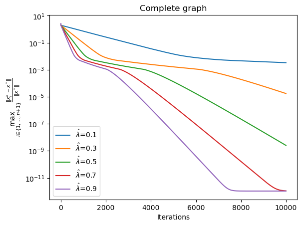
Refer to caption
Refer to caption
Figure 3: Effect of varying λ^\hat{\lambda} on the performance of the complete and sequential graph algorithms.

Now, we compare the performance of three algorithms using γ^=0.1,η^=0.9\hat{\gamma}=0.1,\hat{\eta}=0.9, λ^=0.9\hat{\lambda}=0.9, and α=0.1\alpha=0.1. In Figure 4(a), the data are represented by dots, while the solution obtained by the CVXPY solver and the complete graph algorithm are shown by red solid and green dashed lines, respectively. The result suggests that the complete graph solution successfully detects both regions of gains and losses and matches the solution given by the CVXPY solver mentioned above. The relative error shown in Figure 4(b) indicates that the complete graph converges faster in terms of iteration counts compared to the others. However, this comes at the cost of increased runtime. The sequential graph and star graph algorithms exhibit slightly different at the beginning but nearly identical after that.

Refer to caption
(a) CGH data with solutions obtained by the CVXPY solver and the complete graph algorithm.
Refer to caption
(b) Convergence comparison of the complete graph, sequential graph, and star graph algorithms.
Figure 4: Comparison of the solutions obtained by graph-based algorithms and the CVXPY solver.

We note that the performance of the algorithms can indeed vary depending on the coefficient matrices, as reflected in the numerical experiments. Choosing these matrices is, in general, a nontrivial task that has been studied independently [13, 14]. The primary aim of our numerical experiments is to demonstrate the generality and applicability of the proposed framework. We focus on clarity and accessibility, providing interpretations for specific scenarios rather than performing an exhaustive sensitivity analysis or drawing broad conclusions regarding performance.

Acknowledgements.

The research of MND, MKT and TDT was supported in part by Australian Research Council grant DP230101749.

References

  • [1]
  • [2] A. Åkerman, E. Chenchene, P. Giselsson, and E. Naldi, Splitting the forward-backward algorithm: a full characterization, arXiv:2504.10999.
  • [3] F.J. Aragón-Artacho, R.I. Boţ, and D. Torregrosa-Belén, A primal-dual splitting algorithm for composite monotone inclusions with minimal lifting, Numer. Algorithms 93(1), 103–130 (2023).
  • [4] F.J. Aragón-Artacho, R. Campoy, and C. López-Pastor, Forward-backward algorithms devised by graphs, SIAM J. Optim. 35(4), 2423–2451 (2025).
  • [5] F.J. Aragón-Artacho, Y. Malitsky, M.K. Tam, and D. Torregrosa-Belén, Distributed forward-backward methods for ring networks, Comput. Optim. Appl. 86(3), 845–870 (2023).
  • [6] H. Attouch and M. Théra, A general duality principle for the sum of two operators, J. Convex Anal. 3(1), 1–24 (1996).
  • [7] S. Bartz, M.N. Dao, and H.M. Phan, Conical averagedness and convergence analysis of fixed point algorithms, J. Glob. Optim. 82(2), 351–373 (2022).
  • [8] H.H. Bauschke and P.L. Combettes, Convex Analysis and Monotone Operator Theory in Hilbert Spaces, 2nd ed., Springer, Cham (2017).
  • [9] H.H. Bauschke, W.M. Moursi, and X. Wang, Generalized monotone operators and their averaged resolvents, Math. Program. 189(1-2), 55–74 (2021).
  • [10] R.I. Boţ and C. Hendrich, A Douglas–Rachford type primal-dual method for solving inclusions with mixtures of composite and parallel-sum type monotone operators, SIAM. J. Optim. 23(4), 2541–2565 (2013).
  • [11] K. Bredies, E. Chenchene, D.A. Lorenz, and E. Naldi, Degenerate preconditioned proximal point algorithms, SIAM J. Optim. 32(3), 2376–2401 (2022).
  • [12] L.M Briceño-Arias and P.L. Combettes, A monotone + skew splitting model for composite monotone inclusions in duality, SIAM J. Optim. 21(4), 1230–1250 (2011).
  • [13] R.L. Bassett and P. Barkley, Optimal design of resolvent splitting algorithms, Math. Prog. Comp., (2026).
  • [14] P. Barkley and R.L. Bassett, Coupled adaptable backward-forward-backward resolvent splitting algorithm (CABRA): A matrix-parametrized resolvent splitting method for the sum of maximal monotone and cocoercive operators composed with linear coupling operators, arXiv:2505.13927.
  • [15] A. Chambolle and T. Pock, A first-order primal-dual algorithm for convex problems with applications to imaging, J. Math. Imaging Vis. 40(1), 120–145 (2011).
  • [16] P. Chen, J. Huang, and X. Zhang, A primal–dual fixed point algorithm for convex separable minimization with applications to image restoration, Inverse Probl. 29(2), 25011 (2013).
  • [17] P.L. Combettes and J.-C. Pesquet, Proximal splitting methods in signal processing, in: H.H. Bauschke, R.S. Burachik, P.L. Combettes, V. Elser, D.R. Luke, and H. Wolkowicz (Eds), Fixed-Point Algorithms for Inverse Problems in Science and Engineering, Springer, New York, (2011).
  • [18] P.L. Combettes and J.-C. Pesquet, Primal–dual splitting algorithm for solving inclusions with mixtures of composite, Lipschitzian, and parallel-sum type monotone operators, Set Valued Var. Anal. 20(2), 307–330 (2012).
  • [19] L. Condat, A primal–dual splitting method for convex optimization involving Lipschitzian, proximable and linear composite terms, J. Optim. Theory. Appl. 158(2), 460–479 (2013).
  • [20] M.N. Dao, M.K. Tam, and T.D. Truong, A general approach to distributed operator splitting, J. Math. Anal. Appl. 562(2), 130692 (2026).
  • [21] J. Douglas and H.H. Rachford, On the numerical solution of heat conduction problems in two and three space variables, Trans. Am. Math. Soc. 82(2), 421–439 (1956).
  • [22] Y. Drori, S. Sabach, and M. Teboulle, A simple algorithm for a class of nonsmooth convex-concave saddle-point problems, Oper. Res. Lett. 43(2), 209–214 (2015).
  • [23] P.L. Lions and B. Mercier, Splitting algorithms for the sum of two nonlinear operators, SIAM J. Nume. Anal. 16(6), 964–979 (1979).
  • [24] Y. Malitsky and M.K. Tam, A forward-backward splitting method for monotone inclusions without cocoercivity, SIAM J. Optim. 30(2), 1451–1472 (2020).
  • [25] Y. Malitsky and M.K. Tam, Resolvent splitting for sums of monotone operators with minimal lifting, Math. Program. 201, 231–262 (2023).
  • [26] S. Noschese, L. Pasquini, and L. Reichel, Tridiagonal Toeplitz matrices: properties and novel applications, Numer. Linear Algebra Appl. 20, 302–326 (2013).
  • [27] H. Raguet, J. Fadili, and G. Peyré, A generalized forward-backward splitting, SIAM J. Imaging Sci. 6(3), 1199–1226 (2013).
  • [28] R.T. Rockafellar, Monotone operators associated with saddle-functions and minimax problems, in: F.E. Browder (Ed.) Nonlinear functional analysis, Proc. Symp. Pure Math. 18, 241–250 (1970).
  • [29] R.T. Rockafellar and R. Wets, Variational Analysis, vol. 317. Springer, Berlin (1998).
  • [30] F. Roldán, Forward-primal-dual-half-forward algorithm for splitting four operators, J. Optim. Theory. Appl. 204(1), 11 (2025).
  • [31] E.K. Ryu, Uniqueness of DRS as the 2 operator resolvent-splitting and impossibility of 3 operator resolvent-splitting, Math. Program. 182(1-2), 233–273 (2020).
  • [32] M.K. Tam, Frugal and decentralised resolvent splittings defined by nonexpansive operators, Optim Lett. 18(7), 1541–1559 (2023).
  • [33] R. Tibshirani, P. Wang, Spatial smoothing and hot spot detection for CGH data using the fused lasso, Biostatistics 9(1), 18–29 (2008).
  • [34] R. Tibshirani, M. Saunders, S. Rosset, J. Zhu, and K. Knight, Sparsity and smoothness via the fused lasso, J. R. Stat. Soc. Ser. B (Stat. Methodol.) 67(1), 91–108 (2005).
  • [35] P. Tseng, A modified forward-backward splitting method for maximal monotone mappings, SIAM J. Control Optim. 38(2), 431–446 (2000).
  • [36] B.C. Vũ, A splitting algorithm for dual monotone inclusions involving cocoercive operators, Adv. Comput. Math. 38(3), 667–681 (2013).