Two-dimensional PIC simulation of collective Thomson scattering in a beam-plasma system
Abstract
Collective Thomson scattering (CTS) in a beam-plasma system is reproduced by using 2D PIC simulations and the characteristics of the scattered wave spectrum are examined. By formulating the geometric shape of the scattered wave spectrum in wave number space, where the velocity vector of the beam component and the wave vectors of the incident and scattered waves are arbitrary, it is demonstrated that the spectrum in 2D wave number space becomes asymmetric. The spectrum of scattered waves propagating in a specific direction is presented as a function of wavelength to show that the electron (ion) feature is amplified and becomes asymmetric or distorted when Buneman (ion acoustic) instability occurs. An additional simulation is conducted for a weak, linearly stable beam–plasma system with a hot beam, and confirmed that the obtained scattered wave spectrum shows asymmetric feature. The results are expected to be applicable to the interpretation of radar observations of ionospheric plasmas as well as CTS measurements in laboratory plasmas.
I Introduction
Thomson scattering is used for plasma diagnostics. In laboratory experiments, a laser is injected into the plasma, and the scattered waves are measured to estimate the plasma parameters based on the characteristics of the spectrum. For diagnosing ionospheric plasma, radio waves are used as the incident waves. Thomson scattering in a plasma can be classified into two types depending on the wavelength of the electromagnetic waves. When the wavelength is shorter than the Debye length, it is called noncollective scattering, whereas it is called collective scattering when it is longer. The former results from scattering by thermally fluctuating free electrons, while the latter is caused by electrons reflecting the collective motion of the plasma Froula et al. (2011).
The collective Thomson scattering (CTS) in non-equilibrium plasmas is not yet fully understood, and a comprehensive scattering theory has not been established. Observations of ionospheric plasma using the incoherent scatter radar (ISR) have captured scattered wave spectra that cannot be explained by equilibrium plasma theory Rietveld et al. (1991); Wahlund et al. (1992b, a); Forme et al. (2001); Strømme et al. (2005); Ogawa et al. (2011); Schlatter et al. (2014); Akbari et al. (2017). Moreover, in recent power laser experiments on collisionless shocks Valenzuela-Villaseca et al. (2025); Matsukiyo et al. (2022); Yamazaki et al. (2022); Schaeffer et al. (2019); Rinderknecht et al. (2018); Lebedev et al. (2014) as well as counter-streaming plasma Sakai et al. (2020); Morita et al. (2019); Sakawa et al. (2017); Morita et al. (2013); Ross et al. (2013, 2012); Park et al. (2012), complex scattered wave spectra have also been reported.
To extract meaningful information from such complex CTS spectra, attempts have been made to reproduce CTS spectrum using particle-in-cell (PIC) simulations. Diaz et al. (2008) Diaz et al. (2008) firstly reproduced CTS in an equilibrium plasma. It is well known that the scattered wave spectrum is closely related to the spectral density function, which is the ensemble average of the squared electron density fluctuation spectrum, . Here, is the volume of the plasma, the observation time, the average electron density, and is the scattered wave vector, respectively. They reproduced by performing simulations of a thermal plasma and calculating the Fourier spectrum of the electron density fluctuations. Through long time 2D simulations, by averaging over various wave propagation angles for a specific to increase the number of ensembles sufficiently, they showed that the simulation results were consistent with the theoretical predictions. Subsequently, they performed electrostatic 2D PIC simulations for electron beam-plasma systems, showing that asymmetric or distorted intense scattered wave spectra could be obtained Diaz et al. (2011, 2012). Here, the terms "asymmetric" or "distorted" mean that the scattered wave spectrum exhibits a qualitatively asymmetric shape compared to that in an equilibrium plasma. Their approach is characterized by calculating directly from the simulation without simulating the scattering process.
Sakai et al.(2020,2023) Sakai et al. (2020, 2023) recently proposed a different approach. They reproduced the two-stream instability using 1D PIC simulations and the obtained information of electron and ion density fluctuations (and the incident wave) is used as input to solve the electromagnetic wave equation to simulate CTS. They revealed that resultant scattered wave spectra are highly intense and asymmetric or distorted. It should be noted that, because it is a one-dimensional simulation, the scattering angles in terms of the incident wave are limited to and . Also, in this approach, the absorption of the incident wave by the plasma and the effect of finite size of incident wave packet are not considered.
In this study, we self-consistently reproduce the long time evolution of the beam-plasma system and CTS using 2D PIC simulations. Here, self-consistent means that the evolution of waves in the plasma (both those arising from beam instabilities and those involved in CTS) and the motion of particles (electrons and ions) are solved simultaneously while accounting for their mutual interactions. With actual experimental and observational measurement systems in mind, we discuss the spectrum of scattered waves with a finite scattering angle relative to the incident wave (and a beam velocity). In particular, we investigate how changes in the characteristics of instability due to differences in beam parameters are reflected in the multidimensional scattered wave spectrum.
The paper is organized as follows. Simulation settings are explained in section II. Section III shows the simulation results including 2D CTS spectra and the spectra of the scattered waves propagating in a specific direction for various beam parameters. Then in section IV, we reproduce the CTS in a weak beam-plasma system. Finally, discussions and summary are given in section V.
II Simulation settings

Here, we use a 2D periodic boundary electromagnetic full-PIC simulation of a system consisting of background ions, electrons, and beam ions. We further inject a packet of electromagnetic wave into the system to reproduce the CTS in the beam-plasma system.
The number of spatial grids is 1,024 16,384, with 32 superparticles per species per cell. The grid spacing corresponds to the Debye length, which translates to a system size of 25.6 409.6, where and denote the speed of light and electron plasma frequency. The time step is . The ion-to-electron mass ratio is .
As in Fig.1, the incident electromagnetic wave is a linearly polarized wave packet with monochromatic frequency propagating in the direction along . The wave packet size is set to . Its maximum intensity is , wavenumber is , and frequency is , where and are electron density and temperature.
The simulation is performed in the electron rest frame. The electrons follow a Maxwellian distribution with thermal velocity of , while the background ions and beam ions follow a shifted-Maxwellian distribution. The direction of beam drift velocity is at an angle of relative to the axis. The background ions are also given a drift velocity to cancel the net current.
In the next section, we first present the results of three runs. In Run 1, a two-component equilibrium plasma without a beam is considered, where the ion temperature is equal to the electron temperature (). In Run 2, a beam having a relative density of and a temperature of is added. The beam drift velocity is set to . In Run 3, the beam drift velocity is set to , and both the beam and background ion temperatures are reduced to . The corresponding distribution functions are depicted in Fig.1(c-e).
III 2D spectrum of CTS
III.1 Overview

Fig.2 shows the time evolution of the energy densities of various physical quantities for each run. and are the electromagnetic field components of the incident wave.

In Run 1, there is little change in energy, indicating that plasma heating by the incident wave is negligible. According to linear analysis, Run 2 and Run 3 are expected to exhibit Buneman instability and ion acoustic instability, respectively. Fig.3(a) and 3(c) depict the linear dispersion relation for Run 2 and Run 3, which are obtained by numerically solving the following formulaGary (2005).
| (1) |
Here, is the first order derivative of plasma dispersion function, , and denotes the Debye length of the th species. The solid lines represent the real part of wave frequency, while the dashed lines denote growth rate (its imaginary part). Fig.3(b) and 3(d) show spectrum obtained by performing a spatio-temporal Fourier transform on the component for each run in the time range , extracted along . The amplification of the and components observed in Fig.2(b) and 2(c) is attributed to these instabilities. In Run 2 (Fig.2(b)), although weak, the component is amplified due to the Weibel instability, which is not the focus of this study.
Fig.4 shows the similar spectrum along on the and components for each run in the later time range . In Run 1 (Fig.4(a)), Langmuir waves are clearly observed in spectrum. The weak spectrum in the low-frequency () region corresponds to ion acoustic waves. The component reflects these waves, showing scattered waves. There are three distinct bright regions of frequency along the dispersion relation of light in an equilibrium plasma indicated by the white dotted arrows. One is near the frequency of the incident wave (), while the other two are shifted by approximately the plasma frequency to the higher and lower frequency sides. The former is due to ion acoustic wave scattering, and the latter are due to Langmuir wave scattering. In the theory of CTS, the former is called the ion feature, while the latter is called the electron feature. In Run 2 (Fig.4(b)), as seen in , the beam mode is strongly amplified due to Buneman instability, and accordingly, strong scattering due to this beam mode is also observed in . The strongest signal in the scattered wave spectrum is indicated by the orange arrow (Other scattered signals are indicated by the white dotted arrows). In Run 3 (Fig.4(c)), ion acoustic instability amplifies low-frequency ion acoustic waves in the component, and in response, scattered waves at the frequency near the incident wave are prominently observed in the component. Again, the strongest scattered wave signal is indicated by the orange arrow and other scattered signals are by the white dotted arrows.

III.2 2D CTS spectrum

By performing a Fourier transform of the component data at each time step in the and directions, a spectrum is obtained. Fig.5 shows the time-averaged spectrum obtained over the time range of the simulation for the three runs. Any cross-section of these figures represents the spectrum of scattered light in that direction. Note that due to the symmetry of the Fourier transform, the spectrum is symmetric about the origin.
As seen in Fig.5, the characteristic feature of the spectrum is the presence of multiple ring structures. To understand these structures, we consider the resonance conditions among the incident wave , the scattered waves , and the waves in the plasma . The frequency and wavenumber resonance conditions among these waves are given as follows.
| (2) |
| (3) |
The dispersion relation of the incident and the scattered wave is
| (4) |
The dispersion relations of Langmuir wave, ion acoustic wave, and beam mode are
| (5) |
| (6) |
| (7) |
respectively, where is sound speed.
Substituting eqs.(3)-(5) into eq.(2) gives
| (8) |
Here, has been assumed. Eq.(8) represents the equations of two circles with radii and , corresponding to the outer and the inner dashed circles in Fig.5(d).
Substituting eqs.(3),(4), and (6) into eq.(2), with the assumption , gives
| (9) |
Note that the above equation does not represent concentric circles in contrast to eq.(8). Since , it can be seen that the two circles represented by the above equation are located approximately midway between the two dashed circles represented by eq.(8) in Fig.5(d). The correspondence between Figs.5(d) and 5(a) is clear.
Similarly, substituting eqs.(3),(4), and (7) into eq.(2), with the assumption , gives
| (10) |
This leads to an asymmetric circle in Fig.5(e), explaining the asymmetric spectrum in Fig.5(b). As the beam velocity, , decreases and approaches the sound speed, , it nearly overlaps with the inner circle in Fig.5(d), making it indistinguishable at this scale (Fig.5(f)).
III.3 CTS spectrum with observed format
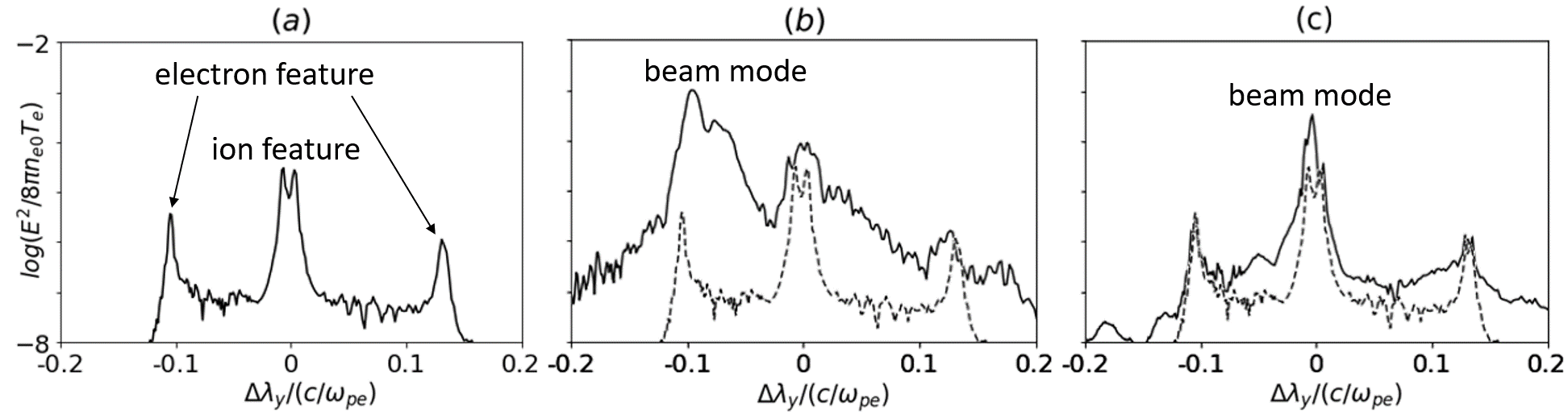
In a laboratory experiment, the spectrum varies depending on the location of the scattered wave detection system. As an example, consider the case where the detection system is placed at -90 degrees relative to the incident wave (in the negative direction). Figs.6(a)-(c) show cross-sections of the spectrum in the region along the axis of Figs.5(a)-(c) for Run 1 to Run 3. Here, the horizontal axis represents the values converted to wavelength and plotted as deviations from the incident wavelength. The dashed lines in Figs.6(b) and 6(c) are for reference and are the same as those in Fig.6(a).
In Fig.6(a), characteristic features of the CTS spectrum of a typical equilibrium plasma can be observed. The double peak near corresponds to the ion feature, while the pair of peaks at both ends represents the electron feature. The slight asymmetry in the electron feature peaks arises because the value of is smaller than that in typical experimental conditions due to constraints in the numerical simulation.
In contrast, in Fig.6(b), the peak corresponding to the electron feature on the short-wavelength side is significantly amplified due to the influence of Buneman instability. In Fig.6(c), the peak corresponding to the ion feature is enhanced due to ion acoustic instability. Upon closer inspection, it can also be seen that the ion feature is strongly amplified on the short-wavelength side. The qualitative spectral features described above have also been confirmed in 1D simulations Sakai et al. (2020, 2023).
IV CTS in a weak beam-plasma system
Using this simulation, we can also reproduce CTS spectra for weak beams that do not lead to instabilities. Here, we consider the case of ion distribution function shown in Fig.7(a), where the beam drift velocity is comparable to the thermal velocity. Since the slope of the distribution function is negative everywhere, no instability arises. Such distribution functions are often thought to be realized in quasi-perpendicular shock transition regions with upstream ion beta of order unity Valenzuela-Villaseca et al. (2025), as well as in ionospheric plasmas accompanied by ion outflows Wahlund et al. (1992a). We set the beam ion thermal velocity to twice that of the background ion thermal velocity (, and the electron thermal velocity to ten times that of the background ions (), with using the same mass ratio 25. The relative drift velocity between the beam ions and electrons is , and that between the background ions and electrons is . The ratio of beam to background ion density is .

Fig.7(b) shows the scattered light spectrum obtained in the same manner as Fig.6. An enlarged view of the ion feature is shown in Fig.7(c), where the vertical axis is in a linear scale. An asymmetric ion feature spectrum is reproduced. A main peak is seen on the longer wavelength side (), with a slightly enhanced signal on the shorter wavelength side (). The intensity ratio of this shorter wavelength signal to the main peak is approximately 0.5. This asymmetric spectrum in Fig.7(b) and 7(c) can be understood as a scattered wave spectrum produced by two ion components with different drift velocities and background electrons.
V Summary and Discussions
We have self-consistently reproduced collective Thomson scattering in a nonequilibrium plasma (beam–plasma system) using two-dimensional PIC simulations and discussed the characteristics of the scattered waves. In a general two-dimensional in-plane configuration where the beam velocity and the propagation direction of the incident wave are not aligned, we examined the wave number spectra of scattered waves propagating in arbitrary directions. While a symmetric two-dimensional wave number spectrum is obtained for an equilibrium plasma without a beam, the beam–plasma system yields an asymmetric spectrum. By taking into account the linear dispersion relations of the incident wave, the scattered waves, and the scattering modes (Langmuir waves, ion acoustic waves, and beam modes), the spectral features can be largely understood. We further performed simulations for a weak, linearly stable beam–plasma system with a hot beam, and confirmed that the obtained scattered wave spectrum shows clear asymmetric feature.
The results obtained in this study, as well as those that can be derived using similar numerical approaches, should be useful for interpreting Thomson scattering measurements of nonequilibrium beam–plasma systems that are frequently observed in both space and laboratory plasmas. In the high-latitude ionosphere, beam instabilities are believed to be driven by auroral precipitating electrons, and indeed, Rietveld et al. (1991)Rietveld et al. (1991) reported asymmetric spectra detected by ISR. In laboratory plasmas as well, recent high-power laser experiments on collisionless shocks often generate localized (ion) beam–plasma systems in the shock transition region and/or developing shock region, where similarly asymmetric scattered wave spectra may arise Valenzuela-Villaseca et al. (2025); Matsukiyo et al. (2022); Schaeffer et al. (2019); Rinderknecht et al. (2018); Lebedev et al. (2014). Although such measurements have traditionally been considered difficult to interpret, we expect that detailed comparison with the numerical data proposed here will enable qualitative and quantitative interpretation. However, several issues still remain, as discussed below.
In laboratory experiments and ionospheric radar observations, the frequency of the incident wave is typically about two orders of magnitude higher than the electron plasma frequency. In the present PIC simulations, however, the incident wave frequency is , and therefore some care is required for making quantitative arguments. In Sakai et al. (2020Sakai et al. (2020),2023Sakai et al. (2023)), the wave equation was solved separately by using electron density fluctuation data obtained from PIC simulations. This approach improves computational efficiency because it avoids solving the incident and scattered waves directly within the PIC simulation. On the other hand, since the nonequilibrium plasma processes and the scattering processes are treated separately, the self-consistency of the model is lost. As seen in Fig.2, in cases where the ratio of the incident wave energy density to the plasma electron thermal energy density is small and plasma heating by the incident wave can be neglected, the method of Sakai et al. (2020Sakai et al. (2020),2023Sakai et al. (2023)) should be effective.
Related to this, a lower frequency of the incident wave also means a longer incident wavelength. In actual experiments and ionospheric observations, it often happens that is on the order of unity, in which case the effects of incoherent scattering cannot be neglected. Milder et al. (2021) Milder et al. (2021) discuss situations where crosses unity depending on the scattering angle. In this sense, the present results, corresponding to , may overestimate the effects of collective scattering.
In this work, the ion to electron mass ratio was set to 25. Employing the real mass ratio would reduce the sound speed excessively, and reproducing the double-peak structure of the ion feature would then require orders-of-magnitude higher resolution in frequency–wavenumber space, which is not practically achievable. Nonetheless, we consider the present method, capable of self-consistently reproducing CTS in non-equilibrium plasmas, to be highly valuable.
In many space plasma environments and laboratory settings, a background magnetic field is present. However, as long as we focus on electrostatic instabilities driven by field-aligned beams and phenomena occurring on spatial scales smaller than the ion gyro radius, we consider that the influence on the ion feature spectrum discussed here is minimal. On the other hand, when electrons are magnetized, the appearance of gyro lines in the scattered wave spectrum has been reported in ionospheric ISR observations.(Bhatt et al., 2006; Akbari et al., 2017) The case presented by Bhatt et al. (2006)Bhatt et al. (2006) shows a plasma line to gyro line intensity ratio of roughly four. In general, gyro lines are weaker than plasma lines, and long integration times are typically required to achieve a sufficient S/N ratio. However, in situations where gyro lines are efficiently excited via some instabilities, they may be detectable more readily, even with relatively short integration times. Verification of such effects remains a subject for future work.
Acknowledgements.
We thank S. Isayama and K. Sakai for fruitful discussions. This research was partially supported by The Kajima Foundation for the International Joint Research Grants (2025-06) and JSPS KAKENHI grant No.23K22558 (SM). The computation was carried out using the computer resource offered under the category of General Projects by Research Institute for Information Technology, Kyushu University.Data Availability Statement
The data that support the findings of this study are available from the corresponding author upon reasonable request.
References
- Space Sci. Rev. 212, pp. 249. Cited by: §I, §V.
- Geophys. Res. Lett. 33, pp. L14105. Cited by: §V.
- J. Geophys. Res. 116, pp. A00K10. Cited by: §I.
- Radio Sci. 43, pp. RS1007. Cited by: §I.
- Ann. Geophys. 30, pp. 1169. Cited by: §I.
- J. Geophys. Res. 106, pp. 21503. Cited by: §I.
- Plasma scattering of electromagnetic radiation. Elsevier Inc.. Cited by: §I.
- Theory of space plasma microinstabilities. CAMBRIDGE UNIVERSITY PRESS. Cited by: §III.1.
- Phys. Plasmas 21, pp. 056305. Cited by: §I, §V.
- Phys. Rev. E 106, pp. 025205. Cited by: §I, §V.
- Phys. Rev. Lett. 127, pp. 015001. Cited by: §V.
- Phys. Plasmas 26, pp. 090702. Cited by: §I.
- Phys. Plasmas 9, pp. 092115. Cited by: §I.
- J. Geophys. Res. 116, pp. A03313. Cited by: §I.
- Hihg Ene. Dens. Phys. 8, pp. 38. Cited by: §I.
- J. Geophys. Res. 96, pp. 19291. Cited by: §I, §V.
- Phys. Rev. Lett. 120, pp. 095001. Cited by: §I, §V.
- Phys. Plasmas 19, pp. 056501. Cited by: §I.
- Phys. Rev. Lett. 110, pp. 145005. Cited by: §I.
- Phys. Plasmas 27, pp. 103104. Cited by: §I, §I, §III.3, §V.
- Phys. Plasmas 30, pp. 012105. Cited by: §I, §III.3, §V.
- High Ene. Dens. Phys. 23, pp. 207. Cited by: §I.
- Phys. Rev. Lett. 122, pp. 245001. Cited by: §I, §V.
- J. Geophys. Res. 119, pp. 8499. Cited by: §I.
- Geophys. Res. Lett. 32, pp. L05103. Cited by: §I.
- arXiv 2509, pp. 12164. Cited by: §I, §IV, §V.
- Geophys. Res. Lett. 19, pp. 1919. Cited by: §I, §IV.
- J. Geophys. Res. 97, pp. 3019. Cited by: §I.
- Phys. Rev. E 105, pp. 025203. Cited by: §I.