跳到论文正文
W Papers独立论文阅读器 arXiv:2512.09273 论文正文 计算阅读时间 · 0%
引用这篇论文根据当前论文元数据生成,正式投稿前建议核对。


On the inverse of covariance matrices for unbalanced crossed designs

Ziyang Lyulabel=e1]Ziyang.Lyu@unsw.edu.au\orcid0000-0003-3307-4148    S.A. Sissonlabel=e2]Scott.Sisson@unsw.edu.au\orcid0000-0001-8943-067X    A.H. Welshlabel=e3]Alan.Welsh@anu.edu.au\orcid0000-0002-3165-9559 UNSW Data Science Hub, and School of Mathematics and Statistics, University of New South Walespresep=, ]e1,e2 Research School of Finance, Actuarial Studies and Statistics, Australian National Universitypresep=, ]e3
Abstract

This paper addresses a long-standing open problem in the analysis of linear mixed models with crossed random effects under unbalanced designs: how to find an analytic expression for the inverse of 𝐕\mathbf{V}, the covariance matrix of the observed response. The inverse matrix 𝐕−1\mathbf{V}^{-1} is required for likelihood-based estimation and inference. However, for unbalanced crossed designs, 𝐕\mathbf{V} is dense and the lack of a closed-form representation for 𝐕−1\mathbf{V}^{-1}, until now, has made using likelihood-based methods computationally challenging and difficult to analyse mathematically. We use the Khatri–Rao product to represent 𝐕\mathbf{V} and then to construct a modified covariance matrix whose inverse admits an exact spectral decomposition. Building on this construction, we obtain an elegant and simple approximation to 𝐕−1\mathbf{V}^{-1} for asymptotic unbalanced designs. For non-asymptotic settings, we derive an accurate and interpretable approximation under mildly unbalanced data and establish an exact inverse representation as a low-rank correction to this approximation, applicable to arbitrary degrees of unbalance. Simulation studies demonstrate the accuracy, stability, and computational tractability of the proposed framework.

Neumann series,
keywords:
[class=MSC]
keywords:
\startlocaldefs\endlocaldefs

, , and

1 Introduction

Linear mixed models with crossed random effects are widely used in education, psychology, and recommender systems, where observations are affected by multiple categorical factors in a fully crossed structure. Unlike nested designs, crossed structures involve non-hierarchical interactions among factors, resulting in complex correlation structures. As a result, the marginal covariance matrix of the observed response, denoted by 𝐕\mathbf{V}, is typically dense. Computing or approximating 𝐕−1\mathbf{V}^{-1} is essential for likelihood-based estimation and inference, including maximum likelihood (ML) estimation, restricted maximum likelihood (REML) estimation, and empirical best linear unbiased prediction (EBLUP), because 𝐕−1\mathbf{V}^{-1} directly determines the form and precision of these procedures.

However, deriving the analytical form of 𝐕−1\mathbf{V}^{-1} for unbalanced crossed designs, where the number of observations varies across cells defined by the factor levels, has been an open problem for more than fifty years. [searle1973wanted] first recognized the challenge of expressing 𝐕−1\mathbf{V}^{-1} in closed form under unbalanced data, and [wansbeek1982another] later proposed a recursive approximation. However, the explicit dependence of its elements on unknown parameters called variance components remains unresolved, and a general analytical or tractable representation of 𝐕−1\mathbf{V}^{-1} is not available.

The highly complex structure of the variance matrix 𝐕\mathbf{V} under unbalanced crossed designs has meant that very few studies focus on crossed random models, and those that do, avoid using likelihood-based methods. For example, the asymptotic analysis of [jiang2025asymptotic] for generalized linear crossed random models employed a second-order Laplace approximation of a conditional expectation to achieve likelihood-free inference that does not require evaluating 𝐕−1\mathbf{V}^{-1}. Other recent studies have, to varying degrees, explored approximations related to 𝐕−1\mathbf{V}^{-1} in simplified crossed random-effects settings. For example, [gao2017efficient] proposed a moment-based method for estimating variance components, and [ghosh2022backfitting] introduced a backfitting algorithm for computing generalized least squares estimators. However, these methods are limited to special cases where each cell contains only one observation and no interaction terms are present, and thus do not address the general structure of 𝐕−1\mathbf{V}^{-1} under arbitrary cell sizes or with interaction effects. Therefore, obtaining an explicit and tractable expression for 𝐕−1\mathbf{V}^{-1} remains one of the central unresolved problems in the theory of crossed mixed models.

We consider data arranged in a two-way table in which the cells correspond to the crossing of two categorical factors, referred to as factor A (rows) and factor B (columns), respectively. Let [yi​j​k,𝐱i​j​k⊤]⊤[y_{ijk},\mathbf{x}_{ijk}^{\top}]^{\top} represent the kkth observed vector in cell (i,j)(i,j), where yi​j​ky_{ijk} is a scalar response variable, and 𝐱i​j​k\mathbf{x}_{ijk} is a pp-dimensional vector of covariates or explanatory variables. Indices ii and jj identify the rows and columns of the table, respectively, and kk identifies the specific observation within a cell. When the number of observations in cell (i,j)(i,j), mi​j≥1m_{ij}\geq 1, the data can be modelled using the two-way crossed random effect with interaction model

yi​j​k=μ​(𝐱i​j​k)+αi+βj+γi​j+ei​j​k,y_{ijk}=\mu(\mathbf{x}_{ijk})+\alpha_{i}+\beta_{j}+\gamma_{ij}+e_{ijk}, (1)

for i=1,…,gi=1,\ldots,g, j=1,…,hj=1,\ldots,h, k=1,…,mi​jk=1,\ldots,m_{ij}, where μ​(𝐱i​j​k)\mu(\mathbf{x}_{ijk}) is the conditional mean or regression function of the response given the covariate 𝐱i​j​k\mathbf{x}_{ijk}, αi\alpha_{i} is the random effect due to the iith row, βj\beta_{j} is the random effect due to the jjth column, γi​j\gamma_{ij} is the interaction random effect for row ii and column jj, and ei​j​ke_{ijk} is the error term. The random variables αi\alpha_{i}, βj\beta_{j}, γi​j\gamma_{ij} and ei​j​ke_{ijk} are assumed mutually independent with zero means and variances σα2\sigma_{\alpha}^{2}, σβ2\sigma_{\beta}^{2}, σγ2\sigma_{\gamma}^{2}, and σe2\sigma_{e}^{2}, respectively. Because our focus is on the random effects, we leave the regression function μ​(𝐱i​j​k)\mu(\mathbf{x}_{ijk}) in general form; see [lyu2024increasing, lyu2025asymptotics] for a useful specific form. The no interaction model assumes σγ2=0{\sigma}_{\gamma}^{2}=0 (and hence γi​j=0\gamma_{ij}=0), which is required for identifiability when mi​j=1m_{ij}=1. Our results in this case follow as a special case of the general model (1).

Under the model (1), the covariance matrix of the response 𝐕\mathbf{V} is dense. For balanced designs, where mi​j=mm_{ij}=m, 𝐕\mathbf{V} can be written using Kronecker products [searle1979dispersion], which facilitates theoretical analysis and explicit matrix inversion. Building on this structure, [lyu2024increasing, lyu2025asymptotics] studied the asymptotic properties of ML and REML estimators and EBLUPs under balanced settings. However, this representation does not hold in unbalanced designs, where the structure of 𝐕\mathbf{V} becomes substantially more complicated. Consequently, obtaining accurate and tractable approximations to 𝐕−1\mathbf{V}^{-1} in general unbalanced settings remains a central challenge, both for computational efficiency and in terms of enabling rigorous asymptotic analysis.

This paper develops a unified framework for approximating and analyzing 𝐕−1\mathbf{V}^{-1} under general unbalanced crossed random effects designs. Section 2 introduces notation and the Khatri–Rao product, a generalization of the Kronecker product. Section 3 defines a modified covariance matrix with a closed-form inverse that yields a tractable approximation to 𝐕−1\mathbf{V}^{-1} under the asymptotic setting and under the non-asymptotic setting with mild unbalance. We also derive an exact expression for a low-rank correction to the approximation under the non-asymptotic setting with severe unbalance. Section 4 presents simulation results that confirm the accuracy of the approximation, and Section 5 concludes with a discussion of the broader implications and possible extensions of this work.

2 Preliminaries

2.1 Khatri–Rao product

To overcome the analytical and computational challenges posed by unbalanced crossed designs, we introduce the Khatri–Rao product [khatri1968solutions, liu2008hadamard], which generalizes the Kronecker product traditionally used with balanced designs. Unlike the Kronecker product, which requires identical replication across cells, the Khatri–Rao product accommodates variation in cell sizes and enables an exact, structured expression for the covariance matrix even when the data are unbalanced. To our knowledge, this is the first use of the Khatri–Rao product to represent unbalanced crossed random effects structures.

Consider matrices 𝐀=(ai​j)\mathbf{A}=(a_{ij}) of order m×nm\times n and 𝐁=(bk​l)\mathbf{B}=(b_{kl}) of order p×qp\times q. Let 𝐀=(𝐀i​j)\mathbf{A}=(\mathbf{A}_{ij}) be partitioned with 𝐀i​j\mathbf{A}_{ij} denoting the (i,j)(i,j)th block submatrix of order mi×njm_{i}\times n_{j}, and 𝐁=(𝐁k​l)\mathbf{B}=(\mathbf{B}_{kl}) be partitioned with 𝐁k​l\mathbf{B}_{kl} denoting the (k,l)(k,l)th block submatrix of order pk×qlp_{k}\times q_{l} (∑imi=m,∑jnj=n,∑kpk=p\sum_{i}m_{i}=m,\sum_{j}n_{j}=n,\sum_{k}p_{k}=p and ∑lql=q\sum_{l}q_{l}=q). Assume that 𝐀\mathbf{A} and 𝐁\mathbf{B} have the same number of row and column partitions. The Khatri–Rao product of two suitably partitioned matrices is then

𝐀⊛𝐁=(𝐀i​j⊗𝐁i​j)i​j,\displaystyle\mathbf{A}\circledast\mathbf{B}=\left(\mathbf{A}_{ij}\otimes\mathbf{B}_{ij}\right)_{ij},

where the (i,j)(i,j)-th block of 𝐀⊛𝐁\mathbf{A}\circledast\mathbf{B} is the Kronecker product of the corresponding blocks 𝐀i​j\mathbf{A}_{ij} and 𝐁i​j\mathbf{B}_{ij}. Specifically, each block 𝐀i​j⊗𝐁i​j\mathbf{A}_{ij}\otimes\mathbf{B}_{ij} has size mi​pi×nj​qjm_{i}p_{i}\times n_{j}q_{j}. The overall size of 𝐀⊛𝐁\mathbf{A}\circledast\mathbf{B} is therefore (∑imi​pi)×(∑jnj​qj)(\sum_{i}m_{i}p_{i})\times(\sum_{j}n_{j}q_{j}). Throughout, ⊗\otimes denotes the Kronecker product, and ⊛\circledast denotes the Khatri–Rao product. For example, if 𝐀\mathbf{A} and 𝐁\mathbf{B} are both partitioned matrices with

𝐀=[𝐀11𝐀12𝐀21𝐀22]=[123456789],𝐁=[𝐁11𝐁12𝐁21𝐁22]=[147258369],\displaystyle\mathbf{A}=\begin{bmatrix}\mathbf{A}_{11}&\mathbf{A}_{12}\\ \mathbf{A}_{21}&\mathbf{A}_{22}\end{bmatrix}=\left[\begin{array}[]{cc|c}1&2&3\\ 4&5&6\\ \hline\cr 7&8&9\end{array}\right],\quad\mathbf{B}=\begin{bmatrix}\mathbf{B}_{11}&\mathbf{B}_{12}\\ \mathbf{B}_{21}&\mathbf{B}_{22}\end{bmatrix}=\left[\begin{array}[]{c|cc}1&4&7\\ \hline\cr 2&5&8\\ 3&6&9\end{array}\right],

then

𝐀⊛𝐁=[𝐀11⊗𝐁11𝐀12⊗𝐁12𝐀21⊗𝐁21𝐀22⊗𝐁22]=[1212214524421416457221245481].\displaystyle\mathbf{A}\circledast\mathbf{B}=\begin{bmatrix}\mathbf{A}_{11}\otimes\mathbf{B}_{11}&\mathbf{A}_{12}\otimes\mathbf{B}_{12}\\ \mathbf{A}_{21}\otimes\mathbf{B}_{21}&\mathbf{A}_{22}\otimes\mathbf{B}_{22}\end{bmatrix}=\left[\begin{array}[]{cc|cc}1&2&12&21\\ 4&5&24&42\\ \hline\cr 14&16&45&72\\ 21&24&54&81\end{array}\right].

2.2 Notation

We define col⁡[⋅]\operatorname{col}[\cdot] to be the column-stacking operator. When stacking vectors indexed by multiple indices, we adopt the convention that the rightmost index varies fastest: for col⁡[𝐱i​j​k]\operatorname{col}[\mathbf{x}_{ijk}], the stacking proceeds from kk, then jj, and finally ii (i.e., 𝐱111,𝐱112,…,𝐱g​h​mg​h\mathbf{x}_{111},\mathbf{x}_{112},\ldots,\mathbf{x}_{ghm_{gh}}). We use the notation (⋅)row(\cdot)_{\mathrm{row}} to mean each row of the matrix is treated as a block submatrix; (⋅)col(\cdot)_{\mathrm{col}} to mean each column is treated as a block submatrix; and (⋅)cell(\cdot)_{\mathrm{cell}} to mean each scalar entry is treated as a block submatrix.

We let the total number of observations be n=∑i=1g∑j=1hmi​jn=\sum_{i=1}^{g}\sum_{j=1}^{h}m_{ij}, and define mL=mini​j⁡(mi​j)m_{L}=\min_{ij}(m_{ij}) and mU=maxi​j⁡(mi​j)m_{U}=\max_{ij}(m_{ij}). Let the vector of cell sizes be 𝐦=[m11,…,mg​h]⊤\mathbf{m}=[m_{11},\ldots,m_{gh}]^{\top}, and define 𝐌=diag⁡(m11,…,mg​h)\mathbf{M}=\operatorname{diag}(m_{11},\ldots,m_{gh}). Let 𝟏a\boldsymbol{1}_{a} denote the aa-dimensional vector of ones and 𝐈a\mathbf{I}_{a} the a×aa\times a identity matrix. To use the Khatri-Rao product effectively, define 𝟏𝐦\boldsymbol{1}_{\mathbf{m}} as the n×1n\times 1 vector of ones, partitioned into g​hgh subvectors as 𝟏𝐦=[𝟏m11⊤,𝟏m12⊤,…,𝟏mg​h⊤]⊤\boldsymbol{1}_{\mathbf{m}}=[\boldsymbol{1}_{m_{11}}^{\top},\boldsymbol{1}_{m_{12}}^{\top},\ldots,\boldsymbol{1}_{m_{gh}}^{\top}]^{\top}, where each 𝟏mi​j\boldsymbol{1}_{m_{ij}} is a vector of ones of length mi​jm_{ij}. Define 𝐈𝐦\mathbf{I}_{\mathbf{m}} as the block-diagonal identity matrix with g​hgh blocks as 𝐈𝐦=diag⁡(𝐈m11,…,𝐈mg​h)\mathbf{I}_{\mathbf{m}}=\operatorname{diag}(\mathbf{I}_{m_{11}},\ldots,\mathbf{I}_{m_{gh}}), where each 𝐈mi​j\mathbf{I}_{m_{ij}} is the mi​j×mi​jm_{ij}\times m_{ij} identity matrix. We define 𝐈𝐦M=diag⁡(m11​𝐈m11,…,mg​h​𝐈mg​h)\mathbf{I}_{\mathbf{m}}^{M}=\operatorname{diag}(m_{11}\mathbf{I}_{m_{11}},\ldots,m_{gh}\mathbf{I}_{m_{gh}}), which can be regarded as the block-diagonal expansion of 𝐌\mathbf{M} onto the observation level. Define 𝐉𝐦=𝟏𝐦​𝟏𝐦⊤\mathbf{J}_{\mathbf{m}}=\boldsymbol{1}_{\mathbf{m}}\boldsymbol{1}_{\mathbf{m}}^{\top} as the n×nn\times n all-ones matrix partitioned as 𝐉𝐦=(𝐉[mi​j:mi′​j′])\mathbf{J}_{\mathbf{m}}=(\mathbf{J}_{[m_{ij}:m_{i^{\prime}j^{\prime}}]}), where each block 𝐉[mi​j:mi′​j′]\mathbf{J}_{[m_{ij}:m_{i^{\prime}j^{\prime}}]} is an mi​j×mi′​j′m_{ij}\times m_{i^{\prime}j^{\prime}} matrix of ones. The block indexed by (i,j)(i,j) in the row direction and (i′,j′)(i^{\prime},j^{\prime}) in the column direction appears at the ((i−1)​h+j,(i′−1)​h+j′)((i-1)h+j,\;(i^{\prime}-1)h+j^{\prime})-th position of the overall g​h×g​hgh\times gh block structure.

We employ two systematic normalizations. The bar-normalization (⋅~\;\tilde{\cdot}\;) rescales each block by the square root of its size, producing unit-length blockwise all-one vectors and projection-type matrices. The tilde-normalization (⋅¯\;\bar{\cdot}\;) instead divides by the block size, producing an averaging operator. Together, these definitions provide a unified way to represent block-structured matrices and streamline subsequent derivations. Specifically, define

𝟏~g=1g​𝟏g,𝟏~h=1h​𝟏h,\displaystyle\tilde{\boldsymbol{1}}_{g}=\frac{1}{\sqrt{g}}\boldsymbol{1}_{g},\quad\tilde{\boldsymbol{1}}_{h}=\frac{1}{\sqrt{h}}\boldsymbol{1}_{h}, 𝟏¯g=1g​𝟏g,𝟏¯h=1h​𝟏h,\displaystyle\bar{\boldsymbol{1}}_{g}=\frac{1}{g}\boldsymbol{1}_{g},\quad\bar{\boldsymbol{1}}_{h}=\frac{1}{h}\boldsymbol{1}_{h},
𝟏~𝐦=[1m11​𝟏m11⊤,…,1mg​h​𝟏mg​h⊤]⊤,\displaystyle\tilde{\boldsymbol{1}}_{\mathbf{m}}=[\frac{1}{\sqrt{m_{11}}}\boldsymbol{1}_{m_{11}}^{\top},\ldots,\frac{1}{\sqrt{m_{gh}}}\boldsymbol{1}_{m_{gh}}^{\top}]^{\top}, 𝟏¯𝐦=[1m11​𝟏m11⊤,…,1mg​h​𝟏mg​h⊤]⊤,\displaystyle\bar{\boldsymbol{1}}_{\mathbf{m}}=[\frac{1}{m_{11}}\boldsymbol{1}_{m_{11}}^{\top},\ldots,\frac{1}{m_{gh}}\boldsymbol{1}_{m_{gh}}^{\top}]^{\top},
𝐈~𝐦=diag⁡(1m11​𝐈m11,…,1mg​h​𝐈mg​h),\displaystyle\tilde{\mathbf{I}}_{\mathbf{m}}=\operatorname{diag}(\frac{1}{\sqrt{m_{11}}}\mathbf{I}_{m_{11}},\ldots,\frac{1}{\sqrt{m_{gh}}}\mathbf{I}_{m_{gh}}), 𝐈¯𝐦=diag⁡(1m11​𝐈m11,…,1mg​h​𝐈mg​h).\displaystyle\bar{\mathbf{I}}_{\mathbf{m}}=\operatorname{diag}(\frac{1}{m_{11}}\mathbf{I}_{m_{11}},\ldots,\frac{1}{m_{gh}}\mathbf{I}_{m_{gh}}).

It then follows that 𝐉~g=𝟏~g​𝟏~g⊤=1g​𝐉g\tilde{\mathbf{J}}_{g}=\tilde{\boldsymbol{1}}_{g}\tilde{\boldsymbol{1}}_{g}^{\top}=\frac{1}{g}\mathbf{J}_{g},  𝐉~h=𝟏~h​𝟏~h⊤=1h​𝐉h\tilde{\mathbf{J}}_{h}=\tilde{\boldsymbol{1}}_{h}\tilde{\boldsymbol{1}}_{h}^{\top}=\frac{1}{h}\mathbf{J}_{h},  𝐉~𝐦=𝟏~𝐦​𝟏~𝐦⊤=𝐈~𝐦​𝐉𝐦​𝐈~𝐦\tilde{\mathbf{J}}_{\mathbf{m}}=\tilde{\boldsymbol{1}}_{\mathbf{m}}\tilde{\boldsymbol{1}}_{\mathbf{m}}^{\top}=\tilde{\mathbf{I}}_{\mathbf{m}}\mathbf{J}_{\mathbf{m}}\tilde{\mathbf{I}}_{\mathbf{m}},  𝐉¯𝐦=𝟏¯𝐦​𝟏¯𝐦⊤=𝐈¯𝐦​𝐉𝐦​𝐈¯𝐦\bar{\mathbf{J}}_{\mathbf{m}}=\bar{\boldsymbol{1}}_{\mathbf{m}}\bar{\boldsymbol{1}}_{\mathbf{m}}^{\top}=\bar{\mathbf{I}}_{\mathbf{m}}\mathbf{J}_{\mathbf{m}}\bar{\mathbf{I}}_{\mathbf{m}}, and 𝐉~𝐦​𝐉~𝐦=g​h​𝐉~𝐦\tilde{\mathbf{J}}_{\mathbf{m}}\tilde{\mathbf{J}}_{\mathbf{m}}=gh\tilde{\mathbf{J}}_{\mathbf{m}}.

The following identities in Lemma 1 will be used throughout the paper. They play a key role in simplifying the analysis of crossed random effects models under unbalanced designs, and enable structural insight into likelihood-based inference and prediction. Other related mixed product properties are presented in Lemma 2, given in the Supplementary Material with illustrative examples.

Lemma 1.

Suppose 𝐚\mathbf{a} is a g×1g\times 1 vector and 𝐛\mathbf{b} is an h×1h\times 1 vector. Let 𝐏\mathbf{P} and 𝐑\mathbf{R} be g×gg\times g matrices, and 𝐐\mathbf{Q} and 𝐒\mathbf{S} be h×hh\times h matrices. Then the following equalities hold.

[(𝐚⊗𝐛)row⊛𝟏~𝐦]⊤​[(𝐏⊗𝐐)cell⊛𝐉~𝐦]=[(𝐚⊤​𝐏)⊗(𝐛⊤​𝐐)]col⊛𝟏~𝐦⊤,\displaystyle\left[(\mathbf{a}\otimes\mathbf{b})_{\mathrm{row}}\circledast\tilde{\boldsymbol{1}}_{\mathbf{m}}\right]^{\top}\left[(\mathbf{P}\otimes\mathbf{Q})_{\mathrm{cell}}\circledast\tilde{\mathbf{J}}_{\mathbf{m}}\right]=[(\mathbf{a}^{\top}\mathbf{P})\otimes(\mathbf{b}^{\top}\mathbf{Q})]_{\mathrm{col}}\circledast\tilde{\boldsymbol{1}}_{\mathbf{m}}^{\top},
[(𝐏⊗𝐐)cell⊛𝐉~𝐦]​[(𝐑⊗𝐒)cell⊛𝐉~𝐦]=[(𝐏𝐑)⊗(𝐐𝐒)]cell⊛𝐉~𝐦,\displaystyle\left[(\mathbf{P}\otimes\mathbf{Q})_{\mathrm{cell}}\circledast\tilde{\mathbf{J}}_{\mathbf{m}}\right]\left[(\mathbf{R}\otimes\mathbf{S})_{\mathrm{cell}}\circledast\tilde{\mathbf{J}}_{\mathbf{m}}\right]=[(\mathbf{P}\mathbf{R})\otimes(\mathbf{Q}\mathbf{S})]_{\mathrm{cell}}\circledast\tilde{\mathbf{J}}_{\mathbf{m}},
[(𝐏⊗𝐐)cell⊛𝐉¯𝐦]​[(𝐑⊗𝐒)cell⊛𝐉¯𝐦]=[(𝐏⊗𝐐)​𝐌−1​(𝐑⊗𝐒)]cell⊛𝐉¯𝐦,\displaystyle\left[(\mathbf{P}\otimes\mathbf{Q})_{\mathrm{cell}}\circledast\bar{\mathbf{J}}_{\mathbf{m}}\right]\left[(\mathbf{R}\otimes\mathbf{S})_{\mathrm{cell}}\circledast\bar{\mathbf{J}}_{\mathbf{m}}\right]=[(\mathbf{P}\otimes\mathbf{Q})\mathbf{M}^{-1}(\mathbf{R}\otimes\mathbf{S})]_{\mathrm{cell}}\circledast\bar{\mathbf{J}}_{\mathbf{m}},
[(𝐏⊗𝐐)cell⊛𝐉¯𝐦​𝐈𝐦f]​[(𝐑⊗𝐒)cell⊛𝐉¯𝐦]=[(𝐏⊗𝐐)​f​(𝐦)​𝐌−1​(𝐑⊗𝐒)]cell⊛𝐉¯𝐦,\displaystyle\left[(\mathbf{P}\otimes\mathbf{Q})_{\mathrm{cell}}\circledast\bar{\mathbf{J}}_{\mathbf{m}}\mathbf{I}_{\mathbf{m}}^{f}\right]\left[(\mathbf{R}\otimes\mathbf{S})_{\mathrm{cell}}\circledast\bar{\mathbf{J}}_{\mathbf{m}}\right]=[(\mathbf{P}\otimes\mathbf{Q})f(\mathbf{m})\mathbf{M}^{-1}(\mathbf{R}\otimes\mathbf{S})]_{\mathrm{cell}}\circledast\bar{\mathbf{J}}_{\mathbf{m}},
[(𝐏⊗𝐐)cell⊛𝐈𝐦f​𝐉¯𝐦]​[(𝐑⊗𝐒)cell⊛𝐉¯𝐦]=[(𝐏⊗𝐐)​𝐌−1​(𝐑⊗𝐒)]cell⊛(𝐈𝐦f​𝐉¯𝐦),\displaystyle\left[(\mathbf{P}\otimes\mathbf{Q})_{\mathrm{cell}}\circledast\mathbf{I}_{\mathbf{m}}^{f}\bar{\mathbf{J}}_{\mathbf{m}}\right]\left[(\mathbf{R}\otimes\mathbf{S})_{\mathrm{cell}}\circledast\bar{\mathbf{J}}_{\mathbf{m}}\right]=[(\mathbf{P}\otimes\mathbf{Q})\mathbf{M}^{-1}(\mathbf{R}\otimes\mathbf{S})]_{\mathrm{cell}}\circledast(\mathbf{I}_{\mathbf{m}}^{f}\bar{\mathbf{J}}_{\mathbf{m}}),

where 𝐈𝐦f=diag⁡(f​(m11)​𝐈m11,…,f​(mg​h)​𝐈mg​h)\mathbf{I}_{\mathbf{m}}^{f}=\operatorname{diag}(f(m_{11})\mathbf{I}_{m_{11}},\ldots,f(m_{gh})\mathbf{I}_{m_{gh}}), f​(𝐦)=diag⁡(f​(m11),…,f​(mg​h))f(\mathbf{m})=\operatorname{diag}(f(m_{11}),\ldots,f(m_{gh})), and f​(mi​j)f(m_{ij}) is a scalar function.

2.3 Matrix form

Let 𝐲=[y111,…,yg​h​mg​h]⊤\mathbf{y}=[y_{111},\ldots,y_{ghm_{gh}}]^{\top}, 𝐗=[𝐱111,…,𝐱g​h​mg​h]⊤\mathbf{X}=[\mathbf{x}_{111},\ldots,\mathbf{x}_{ghm_{gh}}]^{\top}, 𝜶=[α1,…,αg]⊤\boldsymbol{\alpha}=[\alpha_{1},\ldots,\alpha_{g}]^{\top}, 𝜷=[β1,\boldsymbol{\beta}=[\beta_{1},…,βh]⊤,\beta_{h}]^{\top}, 𝜸=[γ11,…,γg​h]⊤\boldsymbol{\gamma}=[\gamma_{11},\ldots,\gamma_{gh}]^{\top}, and 𝐞=[e111,…,eg​h​mg​h]⊤\mathbf{e}=[e_{111},\ldots,e_{ghm_{gh}}]^{\top}. As before, the indices cycle in lexicographic order, with the rightmost index kk varying fastest. The matrix formation of (1) is

𝐲=μ​(𝐗)+𝐙𝐮+𝐞,\displaystyle\mathbf{y}=\mu(\mathbf{X})+\mathbf{Z}\mathbf{u}+\mathbf{e}, (2)

where 𝐮=[𝜶⊤,𝜷⊤,𝜸⊤]⊤\mathbf{u}=[\boldsymbol{\alpha}^{\top},\boldsymbol{\beta}^{\top},\boldsymbol{\gamma}^{\top}]^{\top} and 𝐙=[𝐙1,𝐙2,𝐙3]\mathbf{Z}=[\mathbf{Z}_{1},\mathbf{Z}_{2},\mathbf{Z}_{3}] with 𝐙1=(𝐈g⊗𝟏h)row⊛𝟏𝐦\mathbf{Z}_{1}=(\mathbf{I}_{g}\otimes\boldsymbol{1}_{h})_{\text{row}}\circledast\boldsymbol{1}_{\mathbf{m}}, 𝐙2=(𝟏g⊗𝐈h)row⊛𝟏𝐦\mathbf{Z}_{2}=(\boldsymbol{1}_{g}\otimes\mathbf{I}_{h})_{\text{row}}\circledast\boldsymbol{1}_{\mathbf{m}} and 𝐙3=(𝐈g⊗𝐈h)row⊛𝟏𝐦\mathbf{Z}_{3}=(\mathbf{I}_{g}\otimes\mathbf{I}_{h})_{\text{row}}\circledast\boldsymbol{1}_{\mathbf{m}}. We let 𝜽=[σα2,σβ2,σγ2,σe2]⊤\boldsymbol{\theta}=[{\sigma}_{\alpha}^{2},{\sigma}_{\beta}^{2},{\sigma}_{\gamma}^{2},{\sigma}_{e}^{2}]^{\top}, 𝐆​(𝜽)=Var⁡(𝐮)=diag⁡(σα2​𝐈g,σβ2​𝐈h,σγ2​𝐈g​h)\mathbf{G}(\boldsymbol{\theta})=\operatorname{Var}(\mathbf{u})=\operatorname{diag}({\sigma}_{\alpha}^{2}\mathbf{I}_{g},{\sigma}_{\beta}^{2}\mathbf{I}_{h},{\sigma}_{\gamma}^{2}\mathbf{I}_{gh}) and Var⁡(𝐞)=σe2​𝐈n\operatorname{Var}(\mathbf{e})={\sigma}_{e}^{2}\mathbf{I}_{n}. The covariance matrix of the random effects, 𝐃​(𝜽)=Var⁡(𝐙𝐮)\mathbf{D}(\boldsymbol{\theta})=\operatorname{Var}(\mathbf{Z}\mathbf{u}), can be written as 𝐙𝐆​(𝜽)​𝐙⊤\mathbf{Z}\mathbf{G}(\boldsymbol{\theta})\mathbf{Z}^{\top}. Using the inner and matrix product relations in Lemma 1, the variance-covariance matrix of 𝐲\mathbf{y}, can be expressed using the Khatri-Rao product as

𝐕​(𝜽)=σe2​𝐈n+𝐃​(𝜽),\displaystyle\mathbf{V}(\boldsymbol{\theta})={\sigma}_{e}^{2}\mathbf{I}_{n}+\mathbf{D}(\boldsymbol{\theta}), (3)

where

𝐃​(𝜽)=σα2​(𝐈g⊗𝐉h)cell⊛𝐉𝐦+σβ2​(𝐉g⊗𝐈h)cell⊛𝐉𝐦+σγ2​(𝐈g⊗𝐈h)cell⊛𝐉𝐦.\displaystyle\mathbf{D}(\boldsymbol{\theta})=\sigma_{\alpha}^{2}(\mathbf{I}_{g}\otimes\mathbf{J}_{h})_{\text{cell}}\circledast\mathbf{J}_{\mathbf{m}}+\sigma_{\beta}^{2}(\mathbf{J}_{g}\otimes\mathbf{I}_{h})_{\text{cell}}\circledast\mathbf{J}_{\mathbf{m}}+\sigma_{\gamma}^{2}(\mathbf{I}_{g}\otimes\mathbf{I}_{h})_{\text{cell}}\circledast\mathbf{J}_{\mathbf{m}}. (4)

The variance-covariance matrix for the model (1) without interaction can be obtained by omitting γ\gamma, σγ2{\sigma}_{\gamma}^{2}, and 𝐙3\mathbf{Z}_{3} from the general form. In this paper, we primarily focus on the model with interaction. Results for the model (1) without interaction arise as a special case and are provided in the Supplementary Material. Throughout, we occasionally omit the dependence on 𝜽\boldsymbol{\theta} in the notation for various matrices (such as 𝐃\mathbf{D} and 𝐕\mathbf{V}) when this causes no ambiguity.

3 Inverse Covariance Matrix

3.1 Spectral decomposition of a modified covariance matrix

In the covariance matrix (3), 𝐃\mathbf{D} captures the structured dependence induced by the row and column random effects, while σe2​𝐈n\sigma_{e}^{2}\mathbf{I}_{n} accounts for independent observation-level noise. Specifically, 𝐃\mathbf{D} is a dense, low-rank matrix whose off-diagonal entries reflect correlations between observations sharing a common row or column factor level. In contrast, σe2​𝐈n\sigma_{e}^{2}\mathbf{I}_{n} is a diagonal, full-rank matrix that contributes homogeneous variability across all observations. In balanced designs, where each cell (i,j)(i,j) contains the same number of observations, the structure of 𝐕\mathbf{V} remains relatively regular. However, in unbalanced designs with substantial variation in cell sizes mi​j{m_{ij}}, the interplay between σe2​𝐈n\sigma_{e}^{2}\mathbf{I}_{n} and 𝐃\mathbf{D} becomes increasingly irregular. The lack of alignment between the uniform error structure and heterogeneous replication across cells, together with the fact that 𝐃\mathbf{D} is dense, complicates both theoretical analysis and numerical computation. In particular, the absence of exploitable structure in the combined matrix makes it difficult to derive a closed-form expression for 𝐕−1\mathbf{V}^{-1}.

To address these challenges, we first consider a modified covariance matrix for the model with interaction (1) of the form

𝐕ˇ=σe2mU​𝐈𝐦M+𝐃,where 𝐈𝐦M=diag⁡(m11​𝐈m11,…,mg​h​𝐈mg​h). \check{\mathbf{V}}=\frac{\sigma_{e}^{2}}{m_{U}}\mathbf{I}_{\mathbf{m}}^{M}+\mathbf{D},\quad\text{where $\mathbf{I}_{\mathbf{m}}^{M}=\operatorname{diag}(m_{11}\mathbf{I}_{m_{11}},\ldots,m_{gh}\mathbf{I}_{m_{gh}})$. } (5)

This construction replaces the observation-level noise component with a block-diagonal form that scales according to each cell size. The matrix 𝐕ˇ\check{\mathbf{V}} retains the same correlation structure as 𝐕\mathbf{V} through 𝐃\mathbf{D}, while introducing a smoothed error structure that can also reflect the local sampling density. Importantly, when the design is balanced so that mi​j≡mm_{ij}\equiv m for all i,ji,j, we have σe2/mU​𝐈𝐦M=σe2​𝐈n{\sigma}_{e}^{2}/m_{U}\mathbf{I}_{\mathbf{m}}^{M}={\sigma}_{e}^{2}\mathbf{I}_{n} and hence 𝐕ˇ=𝐕\check{\mathbf{V}}=\mathbf{V}. Thus, 𝐕ˇ\check{\mathbf{V}} preserves the key features of the original model while enabling a form that is analytically more tractable in unbalanced designs.

To study 𝐕−1\mathbf{V}^{-1} in the analytically challenging general setting, we begin by deriving an explicit expression for 𝐕ˇ−1\check{\mathbf{V}}^{-1}. This provides a tractable starting point for studying 𝐕−1\mathbf{V}^{-1}. Since the only difference between 𝐕ˇ\check{\mathbf{V}} and 𝐕\mathbf{V} lies in the diagonal noise component, this discrepancy plays a key role in the approximation accuracy. All proof details can be found in the Appendix and Supplementary Material.

Let 𝝉αi=[ταi,1,…,ταi,g]⊤\boldsymbol{\tau}_{\alpha_{i}}=[\tau_{\alpha_{i,1}},\ldots,\tau_{\alpha_{i,g}}]^{\top}, i=1,…,g−1i=1,\ldots,g-1, be g−1g-1 orthonormal vectors, each of dimension g×1g\times 1, which are orthogonal to 𝟏g\boldsymbol{1}_{g}, so that

𝟏g⊤​𝝉αi\displaystyle\boldsymbol{1}_{g}^{\top}\boldsymbol{\tau}_{\alpha_{i}} =∑s=1gταi,s=0,\displaystyle=\sum_{s=1}^{g}\tau_{\alpha_{i,s}}=0, and ​𝝉αi′⊤​𝝉αi=∑s=1gταi,s​ταi′,s={1if ​i=i′0if ​i≠i′for ​i,i′=1,…,g−1.\displaystyle\text{and }\boldsymbol{\tau}_{\alpha_{i^{\prime}}}^{\top}\boldsymbol{\tau}_{\alpha_{i}}=\sum_{s=1}^{g}\tau_{\alpha_{i,s}}\tau_{\alpha_{i^{\prime},s}}=\begin{cases}1&\text{if }i=i^{\prime}\\ 0&\text{if }i\neq i^{\prime}\end{cases}\quad\text{for }i,i^{\prime}=1,\ldots,g-1. (6)

Let 𝝉βj=[τβj,1,…,τβj,h]⊤\boldsymbol{\tau}_{\beta_{j}}=[\tau_{\beta_{j,1}},\ldots,\tau_{\beta_{j,h}}]^{\top}, j=1,…,h−1j=1,\ldots,h-1, be h−1h-1 orthonormal vectors, each of dimension h×1h\times 1, which are orthogonal to 𝟏h\boldsymbol{1}_{h}. Similarly, let 𝝉γ,(i,j,k)=[𝝉i,j,k(1,1)⊤,…,𝝉i,j,k(g,h)⊤]⊤\boldsymbol{\tau}_{\gamma,(i,j,k)}=[\boldsymbol{\tau}_{i,j,k}^{(1,1)\top},\ldots,\boldsymbol{\tau}_{i,j,k}^{(g,h)\top}]^{\top}, i=1,…,g;j=1,…,h;k=1,…,mi​j−1i=1,\ldots,g;\,j=1,\ldots,h;\,k=1,\ldots,m_{ij}-1, be ∑i=1g∑j=1h(mi​j−1)\sum_{i=1}^{g}\sum_{j=1}^{h}(m_{ij}-1) vectors, each of dimension n×1n\times 1, where each component 𝝉i,j,k(s,t)\boldsymbol{\tau}_{i,j,k}^{(s,t)} is an ms​t×1m_{st}\times 1 vector defined as 𝝉i,j,k(s,t)=[τ(i,j,k),1(s,t),…,τ(i,j,k),ms​t(s,t)]⊤\boldsymbol{\tau}_{i,j,k}^{(s,t)}=[\tau_{(i,j,k),1}^{(s,t)},\ldots,\tau_{(i,j,k),m_{st}}^{(s,t)}]^{\top}, for s=1,…,g;t=1,…,hs=1,\ldots,g;\,t=1,\ldots,h. Each 𝝉i,j,k(s,t)\boldsymbol{\tau}_{i,j,k}^{(s,t)} is orthonormal and orthogonal to 𝟏ms​t\boldsymbol{1}_{m_{st}}. We can always find such sets of vectors.

Let 𝐂\mathbf{C} be a n×nn\times n matrix partitioned as 𝐂⊤=col⁡[𝐂1,𝐂2,…,𝐂8]\mathbf{C}^{\top}=\operatorname{col}[\mathbf{C}_{1},\mathbf{C}_{2},\ldots,\mathbf{C}_{8}], with 𝐂1\mathbf{C}_{1}–𝐂8\mathbf{C}_{8} defined in Table 1.

Table 1: Definition and dimension of blocks in the partition of 𝐂\mathbf{C}.
Block Definition Dimension
𝐂1\mathbf{C}_{1} (𝟏~g⊗𝟏~h)row⊛𝟏~𝐦(\tilde{\boldsymbol{1}}_{g}\otimes\tilde{\boldsymbol{1}}_{h})_{\text{row}}\circledast\tilde{\boldsymbol{1}}_{\mathbf{m}} n×1n\times 1
𝐂2\mathbf{C}_{2} col[(𝟏~g⊗𝟏~h)row⊛𝝉γ,(g,h,k)]k=1mg​h−1\operatorname{col}\left[(\tilde{\boldsymbol{1}}_{g}\otimes\tilde{\boldsymbol{1}}_{h})_{\text{row}}\circledast\boldsymbol{\tau}_{\gamma,(g,h,k)}\right]_{k=1}^{m_{gh}-1} n×(mg​h−1)n\times(m_{gh}-1)
𝐂3\mathbf{C}_{3} col[(𝟏~g⊗𝝉βj)row⊛𝟏~𝐦]j=1h−1\operatorname{col}\left[(\tilde{\boldsymbol{1}}_{g}\otimes\boldsymbol{\tau}_{\beta_{j}})_{\text{row}}\circledast\tilde{\boldsymbol{1}}_{\mathbf{m}}\right]_{j=1}^{h-1} n×(h−1)n\times(h-1)
𝐂4\mathbf{C}_{4} col[(𝟏~g⊗𝝉βj)row⊛𝝉γ,(g,j,k)]j=1,…,h−1k=1,…,mg​j−1\operatorname{col}\left[(\tilde{\boldsymbol{1}}_{g}\otimes\boldsymbol{\tau}_{\beta_{j}})_{\text{row}}\circledast\boldsymbol{\tau}_{\gamma,(g,j,k)}\right]_{\begin{subarray}{c}j=1,\ldots,h-1\\ k=1,\ldots,m_{gj}-1\end{subarray}} n×∑j=1h−1(mg​j−1)n\times\sum_{j=1}^{h-1}(m_{gj}-1)
𝐂5\mathbf{C}_{5} col[(𝝉αi⊗𝟏~h)row⊛𝟏~𝐦]i=1g−1\operatorname{col}\left[(\boldsymbol{\tau}_{\alpha_{i}}\otimes\tilde{\boldsymbol{1}}_{h})_{\text{row}}\circledast\tilde{\boldsymbol{1}}_{\mathbf{m}}\right]_{i=1}^{g-1} n×(g−1)n\times(g-1)
𝐂6\mathbf{C}_{6} col[(𝝉αi⊗𝟏~h)row⊛𝝉γ,(i,h,k)]i=1,…,g−1k=1,…,mi​h−1\operatorname{col}\left[(\boldsymbol{\tau}_{\alpha_{i}}\otimes\tilde{\boldsymbol{1}}_{h})_{\text{row}}\circledast\boldsymbol{\tau}_{\gamma,(i,h,k)}\right]_{\begin{subarray}{c}i=1,\ldots,g-1\\ k=1,\ldots,m_{ih}-1\end{subarray}} n×∑i=1g−1(mi​h−1)n\times\sum_{i=1}^{g-1}(m_{ih}-1)
𝐂7\mathbf{C}_{7} col[(𝝉αi⊗𝝉βj)row⊛𝟏~𝐦]i=1,j=1g−1,h−1\operatorname{col}\left[(\boldsymbol{\tau}_{\alpha_{i}}\otimes\boldsymbol{\tau}_{\beta_{j}})_{\text{row}}\circledast\tilde{\boldsymbol{1}}_{\mathbf{m}}\right]_{i=1,j=1}^{g-1,h-1} n×(g−1)​(h−1)n\times(g-1)(h-1)
𝐂8\mathbf{C}_{8} col[(𝝉αi⊗𝝉βj)row⊛𝝉γ,(i,j,k)]i=1,…,g−1j=1,…,h−1k=1,…,mi​j−1\operatorname{col}\left[(\boldsymbol{\tau}_{\alpha_{i}}\otimes\boldsymbol{\tau}_{\beta_{j}})_{\text{row}}\circledast\boldsymbol{\tau}_{\gamma,(i,j,k)}\right]_{\begin{subarray}{c}i=1,\ldots,g-1\\ j=1,\ldots,h-1\\ k=1,\ldots,m_{ij}-1\end{subarray}} n×∑i=1g−1∑j=1h−1(mi​j−1)n\times\sum_{i=1}^{g-1}\sum_{j=1}^{h-1}(m_{ij}-1)

The dimension of 𝐂\mathbf{C} is n×nn\times n, because

n=∑i=1g∑j=1hmi​j=\displaystyle n=\sum_{i=1}^{g}\sum_{j=1}^{h}m_{ij}= 1+(mg​h−1)+(h−1)+∑j=1h−1(mg​j−1)+(g−1)\displaystyle 1+(m_{gh}-1)+(h-1)+\sum_{j=1}^{h-1}(m_{gj}-1)+(g-1)
+∑i=1g−1(mi​h−1)+(g−1)​(h−1)+∑i=1g−1∑j=1h−1(mi​j−1).\displaystyle+\sum_{i=1}^{g-1}(m_{ih}-1)+(g-1)(h-1)+\sum_{i=1}^{g-1}\sum_{j=1}^{h-1}(m_{ij}-1).

We can now prove the following theorem which gives the spectral decomposition of the matrix mU​𝐈~𝐦​𝐕ˇ​𝐈~𝐦m_{U}\tilde{\mathbf{I}}_{\mathbf{m}}\check{\mathbf{V}}\tilde{\mathbf{I}}_{\mathbf{m}}. A detailed proof is provided in Appendix A.1.

Theorem 1.

Let 𝛕αi\boldsymbol{\tau}_{\alpha_{i}} (i=1,…,g−1i=1,\ldots,g-1), 𝛕βj\boldsymbol{\tau}_{\beta_{j}} (j=1,…,h−1j=1,\ldots,h-1), and 𝛕γ,(i,j,k)\boldsymbol{\tau}_{\gamma,(i,j,k)} (i=1,…,g;j=1,…,h;k=1,…,mi​j−1i=1,\ldots,g;\,j=1,\ldots,h;\,k=1,\ldots,m_{ij}-1) be the orthonormal vectors defined above. Let 𝐂\mathbf{C} be the n×nn\times n orthogonal matrix with 𝐂⊤=[𝐂1,…,𝐂8]\mathbf{C}^{\top}=[\mathbf{C}_{1},\ldots,\mathbf{C}_{8}], where each block 𝐂i\mathbf{C}_{i} is specified in Table 1. Then 𝐂⊤​𝐂=𝐈n\mathbf{C}^{\top}\mathbf{C}=\mathbf{I}_{n}. For the model with interaction in (1), we have

mU​𝐂​𝐈~𝐦​𝐕ˇ​𝐈~𝐦​𝐂⊤\displaystyle m_{U}\mathbf{C}\tilde{\mathbf{I}}_{\mathbf{m}}\check{\mathbf{V}}\tilde{\mathbf{I}}_{\mathbf{m}}\mathbf{C}^{\top}
=diag[λ1,λ0𝐈[mg​h−1:mg​h−1],λ3𝐈h−1,λ0𝐈[∑j=1h−1(mg​j−1):∑j=1h−1(mg​j−1)],λ5𝐈g−1,\displaystyle=\operatorname{diag}\bigl[\lambda_{1},\,\lambda_{0}\mathbf{I}_{[m_{gh}-1:m_{gh}-1]},\,\lambda_{3}\mathbf{I}_{h-1},\,\lambda_{0}\mathbf{I}_{[\sum_{j=1}^{h-1}(m_{gj}-1):\sum_{j=1}^{h-1}(m_{gj}-1)]},\,\lambda_{5}\mathbf{I}_{g-1},
λ0𝐈[∑i=1g−1(mi​h−1):∑i=1g−1(mi​h−1)],λ7𝐈(g−1)​(h−1),λ0𝐈[∑i=1g−1∑j=1h−1(mi​j−1):∑i=1g−1∑j=1h−1(mi​j−1)]]\displaystyle\quad\lambda_{0}\mathbf{I}_{[\sum_{i=1}^{g-1}(m_{ih}-1):\sum_{i=1}^{g-1}(m_{ih}-1)]},\,\lambda_{7}\mathbf{I}_{(g-1)(h-1)},\,\lambda_{0}\mathbf{I}_{[\sum_{i=1}^{g-1}\sum_{j=1}^{h-1}(m_{ij}-1):\sum_{i=1}^{g-1}\sum_{j=1}^{h-1}(m_{ij}-1)]}\bigr]
=𝚲λ,\displaystyle=\boldsymbol{\Lambda}_{\lambda},

where the five distinct characteristic roots of mU​𝐈~𝐦​𝐕ˇ​𝐈~𝐦m_{U}\tilde{\mathbf{I}}_{\mathbf{m}}\check{\mathbf{V}}\tilde{\mathbf{I}}_{\mathbf{m}} are λ0=σe2\lambda_{0}={\sigma}_{e}^{2}, λ1=σe2+mU​σγ2+h​mU​σα2+g​mU​σβ2\lambda_{1}={\sigma}_{e}^{2}+m_{U}\sigma_{\gamma}^{2}+hm_{U}\sigma_{\alpha}^{2}+gm_{U}\sigma_{\beta}^{2}, λ3=σe2+mU​σγ2+h​mU​σα2\lambda_{3}={\sigma}_{e}^{2}+m_{U}\sigma_{\gamma}^{2}+hm_{U}\sigma_{\alpha}^{2}, λ5=σe2+mU​σγ2+g​mU​σβ2\lambda_{5}={\sigma}_{e}^{2}+m_{U}\sigma_{\gamma}^{2}+gm_{U}\sigma_{\beta}^{2}, and λ7=σe2+mU​σγ2\lambda_{7}={\sigma}_{e}^{2}+m_{U}\sigma_{\gamma}^{2}.

The purpose of weighting the modified covariance matrix 𝐕ˇ\check{\mathbf{V}} is to eliminate the effect of heterogeneous cell sizes, and enable the use of the Khatri–Rao product properties established in Lemmas 1 and 2. After obtaining the eigenvalues of mU​𝐈~𝐦​𝐕ˇ​𝐈~𝐦m_{U}\tilde{\mathbf{I}}_{\mathbf{m}}\check{\mathbf{V}}\tilde{\mathbf{I}}_{\mathbf{m}} via Theorem 1, its inverse can be computed explicitly. The inverse 𝐕ˇ−1\check{\mathbf{V}}^{-1} is then recovered by multiplying by the diagonal matrix 𝐈~𝐦−1\tilde{\mathbf{I}}_{\mathbf{m}}^{-1} as shown in Corollary 2. Detailed derivations are provided in Appendix A.2.

Corollary 2.

Let 𝐉~a0=𝐈a\tilde{\mathbf{J}}_{a}^{0}=\mathbf{I}_{a} and 𝐉~a1=𝐉~a\tilde{\mathbf{J}}_{a}^{1}=\tilde{\mathbf{J}}_{a}. Consider the inverse of the modified covariance 𝐕ˇ\check{\mathbf{V}} in (5) for the model with interaction (1), denoted by 𝐕ˇ−1\check{\mathbf{V}}^{-1}. Then, from Theorem 1, we have

𝐕ˇ−1=mUλ0​𝐈¯𝐦+mU​[∑𝐢=𝟎2𝟏2δi1​i2​(𝐉~gi1⊗𝐉~hi2)]cell⊛𝐉¯𝐦,\displaystyle\check{\mathbf{V}}^{-1}=\frac{m_{U}}{\lambda_{0}}\bar{\mathbf{I}}_{\mathbf{m}}+m_{U}\left[\sum_{\mathbf{i}=\boldsymbol{0}_{2}}^{\boldsymbol{1}_{2}}\delta_{i_{1}i_{2}}(\tilde{\mathbf{J}}_{g}^{i_{1}}\otimes\tilde{\mathbf{J}}_{h}^{i_{2}})\right]_{\text{cell}}\circledast\bar{\mathbf{J}}_{\mathbf{m}}, (7)

where δ00=1/λ7−1/λ0\delta_{00}={1}/{\lambda_{7}}-1/{\lambda_{0}}, δ01=1/λ5−1/λ7\delta_{01}={1}/{\lambda_{5}}-{1}/{\lambda_{7}},δ10=1/λ3−1/λ7\delta_{10}={1}/{\lambda_{3}}-{1}/{\lambda_{7}} and δ11=1/λ1−1/λ3−1/λ5+1/λ7\delta_{11}={1}/{\lambda_{1}}-{1}/{\lambda_{3}}-{1}/{\lambda_{5}}+{1}/{\lambda_{7}}. Here, the exponents i1i_{1} and i2i_{2} are also used as subscripts of δ\delta for notational convenience and readability. They are treated as components of the binary vector 𝐢\mathbf{i}, with the subscripts written in reverse natural order to allow interpretation of 𝐢\mathbf{i} as binary numbers. The summation ∑𝐢=𝟎2𝟏2\sum_{\mathbf{i}=\boldsymbol{0}_{2}}^{\boldsymbol{1}_{2}} denotes the sum over all four binary vectors from 0000 to 1111.

We now make some remarks on Corollary 2.

  1. 1.

    In studying the asymptotic properties of estimators (such as ML and REML estimators), we usually require g,h→∞g,h\to\infty. In this situation, we can obtain an approximation to (7), namely

    𝐕ˇ−1=mUλ0​𝐈¯𝐦+(mUλ7−mUλ0)​(𝐈g⊗𝐈h)cell⊛𝐉¯𝐦+𝐎[n:n]​(1min⁡(g,h)​mL2),\check{\mathbf{V}}^{-1}=\frac{m_{U}}{\lambda_{0}}\bar{\mathbf{I}}_{\mathbf{m}}+(\frac{m_{U}}{\lambda_{7}}-\frac{m_{U}}{\lambda_{0}})(\mathbf{I}_{g}\otimes\mathbf{I}_{h})_{\text{cell}}\circledast\bar{\mathbf{J}}_{\mathbf{m}}+\mathbf{O}_{[n:n]}\left(\frac{1}{\min(g,h)m_{L}^{2}}\right), (8)

    where 𝐎[n:n]​(a)\mathbf{O}_{[n:n]}(a) denotes an n×nn\times n matrix with all entries of order O​(a)O(a). Details of the derivation for (8) are provided in the proof of Lemma 4 in Appendix B.2. We retain mLm_{L} in the remainder term even though it is finite, as this choice facilitates extensions to settings where mL→∞m_{L}\to\infty. In this paper, however, we focus on the case where the minimum cell size mLm_{L} is finite, which is more relevant.

  2. 2.

    Under the balanced design where mi​j=mm_{ij}=m for all ii and jj, we have 𝐕=𝐕ˇ\mathbf{V}=\check{\mathbf{V}} and hence 𝐕−1=𝐕ˇ−1\mathbf{V}^{-1}=\check{\mathbf{V}}^{-1}. In this case, we can rewrite (7) as

    𝐕−1=\displaystyle\mathbf{V}^{-1}= 1λ0​[𝐈g⊗𝐈h⊗(𝐈m−𝐉~m)]+1λ7​[(𝐈g−𝐉~g)⊗(𝐈h−𝐉~h)⊗𝐉~m]\displaystyle\frac{1}{\lambda_{0}}[\mathbf{I}_{g}\otimes\mathbf{I}_{h}\otimes(\mathbf{I}_{m}-\tilde{\mathbf{J}}_{m})]+\frac{1}{\lambda_{7}}[(\mathbf{I}_{g}-\tilde{\mathbf{J}}_{g})\otimes(\mathbf{I}_{h}-\tilde{\mathbf{J}}_{h})\otimes\tilde{\mathbf{J}}_{m}]
    +1λ3​[(𝐈g−𝐉~g)⊗𝐉~h⊗𝐉~m]+1λ5​[𝐉~g⊗(𝐈h−𝐉~h)⊗𝐉~m]+1λ1​[𝐉~g⊗𝐉~h⊗𝐉~m],\displaystyle+\frac{1}{\lambda_{3}}[(\mathbf{I}_{g}-\tilde{\mathbf{J}}_{g})\otimes\tilde{\mathbf{J}}_{h}\otimes\tilde{\mathbf{J}}_{m}]+\frac{1}{\lambda_{5}}[\tilde{\mathbf{J}}_{g}\otimes(\mathbf{I}_{h}-\tilde{\mathbf{J}}_{h})\otimes\tilde{\mathbf{J}}_{m}]+\frac{1}{\lambda_{1}}[\tilde{\mathbf{J}}_{g}\otimes\tilde{\mathbf{J}}_{h}\otimes\tilde{\mathbf{J}}_{m}], (9)

    which coincides with the expression given in [searle1979dispersion]. Thus, the exact inverse 𝐕−1\mathbf{V}^{-1} under the balanced case can be viewed as a special case of the inverse of the modified covariance matrix 𝐕ˇ−1\check{\mathbf{V}}^{-1}. The expression (9) has been utilized in recent studies (e.g., [lyu2024increasing, lyu2025asymptotics]) to derive the asymptotic properties of ML and REML estimators as well as EBLUPs.

  3. 3.

    For more general models, such as kk-way crossed random-effects models with unbalanced designs (k≥2k\geq 2), the above approach continues to apply. One only needs to construct 2k2^{k} block matrices following the rule summarized in Table 1. This yields a similar spectral decomposition for the modified covariance matrix and its inverse. The subsequent methodology for approximation and analysis of 𝐕−1\mathbf{V}^{-1} can then be extended to kk-way crossed random-effects models with unbalanced designs.

3.2 Inverse of covariance matrix 𝐕\mathbf{V}

Under unbalanced designs (mi​j≠mm_{ij}\neq m), 𝐕−1\mathbf{V}^{-1} no longer admits an elegant closed form such as (9), since 𝐕=𝐕ˇ+σe2​𝐈𝐦Δ\mathbf{V}=\check{\mathbf{V}}+{\sigma}_{e}^{2}\mathbf{I}_{\mathbf{m}}^{\Delta} with 𝐈𝐦Δ=diag⁡[(1−mi​j/mU)​𝐈mi​j]\mathbf{I}_{\mathbf{m}}^{\Delta}=\operatorname{diag}[(1-m_{ij}/m_{U})\mathbf{I}_{m_{ij}}], and the heterogeneity in cell sizes cannot be eliminated from 𝐈𝐦Δ\mathbf{I}_{\mathbf{m}}^{\Delta}. In this section, we explore the analytic structure of 𝐕−1\mathbf{V}^{-1} from that of 𝐕ˇ−1\check{\mathbf{V}}^{-1} under asymptotic and non-asymptotic cases.

We first consider the asymptotic setting where g,h→∞g,h\to\infty and mLm_{L} is finite (or diverging to infinity). In this case, 𝐕ˇ−1\check{\mathbf{V}}^{-1} admits a block-diagonal approximation as in (8), which provides insight into the form of 𝐕−1\mathbf{V}^{-1}. The following approximation is critical for analyzing the property of likelihood-based estimators and inferences.

Theorem 3.

Suppose g,h→∞g,h\to\infty and all variance components are bounded. Then

𝐕−1=1σe2​𝐈n−σγ2σe2​diag⁡[1σe2+mi​j​σγ2​𝐉mi​j]+𝐎[n:n]​(1min⁡(g1−ε,h1−ε)​mL2),\displaystyle\mathbf{V}^{-1}=\frac{1}{{\sigma}_{e}^{2}}\mathbf{I}_{n}-\frac{{\sigma}_{\gamma}^{2}}{{\sigma}_{e}^{2}}\operatorname{diag}\left[\frac{1}{{\sigma}_{e}^{2}+m_{ij}{\sigma}_{\gamma}^{2}}\mathbf{J}_{m_{ij}}\right]+\mathbf{O}_{[n:n]}\!\left(\frac{1}{\min(g^{1-\varepsilon},h^{1-\varepsilon})m_{L}^{2}}\right), (10)

where 0≤ε<10\leq\varepsilon<1. When σe2/(2​mL2​σγ2)≤1{\sigma}_{e}^{2}/(2m_{L}^{2}{\sigma}_{\gamma}^{2})\leq 1 or mi​j=mm_{ij}=m, we have ε=0\varepsilon=0.

Theorem 3 provides a block-diagonal representation of 𝐕−1\mathbf{V}^{-1} that can substantially simplify the asymptotic analysis of likelihood-based estimation and prediction. This approximation retains only the two leading terms and permits the direct use of the properties of Khatri–Rao products in simplifying the associated estimating equations. Moreover, this exact analytic form greatly improves computational efficiency. When mi​j=mm_{ij}=m, the expression in (10) simplifies to

𝐕−1=1σe2​𝐈n−σγ2σe2​(σe2+m​σγ2)​(𝐈g⊗𝐈h⊗𝐉m)+𝐎[n:n]​(1min⁡(g,h)​m2),\displaystyle\mathbf{V}^{-1}=\frac{1}{{\sigma}_{e}^{2}}\mathbf{I}_{n}-\frac{{\sigma}_{\gamma}^{2}}{{\sigma}_{e}^{2}({\sigma}_{e}^{2}+m{\sigma}_{\gamma}^{2})}(\mathbf{I}_{g}\otimes\mathbf{I}_{h}\otimes\mathbf{J}_{m})+\mathbf{O}_{[n:n]}\!\left(\frac{1}{\min(g,h)m^{2}}\right),

which coincides with (9) as g,h→∞g,h\to\infty.

Although the resulting form (10) is surprisingly elegant and simple, deriving this approximation involves substantial algebraic effort. In brief, by the Woodbury matrix identity,

𝐕−1=(𝐕ˇ+σe2​𝐈𝐦Δ)−1=𝐕ˇ−1−𝐕ˇ−1​(1σe2​𝐈𝐦Δ−1+𝐕ˇ−1)−1​𝐕ˇ−1.\displaystyle\mathbf{V}^{-1}=(\check{\mathbf{V}}+{\sigma}_{e}^{2}\mathbf{I}_{\mathbf{m}}^{\Delta})^{-1}=\check{\mathbf{V}}^{-1}-\check{\mathbf{V}}^{-1}\Bigl(\frac{1}{{\sigma}_{e}^{2}}\mathbf{I}_{\mathbf{m}}^{\Delta-1}+\check{\mathbf{V}}^{-1}\Bigr)^{-1}\check{\mathbf{V}}^{-1}. (11)

Given the explicit expression for 𝐕ˇ−1\check{\mathbf{V}}^{-1} in Corollary 2, the key task is to obtain an analytic expression for (1/σe2​𝐈𝐦Δ−1+𝐕ˇ−1)−1(1/{{\sigma}_{e}^{2}}\mathbf{I}_{\mathbf{m}}^{\Delta-1}+\check{\mathbf{V}}^{-1})^{-1}. Following equation (8) as g,h→∞g,h\to\infty, the term 1/σe2​𝐈𝐦Δ−1+𝐕ˇ−11/{{\sigma}_{e}^{2}}\mathbf{I}_{\mathbf{m}}^{\Delta-1}+\check{\mathbf{V}}^{-1} can be decomposed into a block-diagonal matrix, denoted by 𝐔2\mathbf{U}_{2}, together with a remainder term 𝐎[n:n]​(1/[min⁡(g,h)​mL2])\mathbf{O}_{[n:n]}(1/[\min(g,h)m_{L}^{2}]). The classical truncated Neumann series, commonly used for approximate matrix inversion, cannot be applied here, since it requires the operator norm (or spectral radius) of the perturbation to satisfy ‖𝐔2−1​𝐎[n:n]​(1/[min⁡(g,h)​mL2])‖<1\|\mathbf{U}_{2}^{-1}\mathbf{O}_{[n:n]}(1/[\min(g,h)m_{L}^{2}])\|<1. This condition fails in the asymptotic setting because the matrix dimension diverges as g,h→∞g,h\to\infty, while each entry of the remainder matrix is of order 1/[min⁡(g,h)​mL2]1/[\min(g,h)m_{L}^{2}]. We overcome this difficulty by exploiting the properties of Khatri–Rao products, which ensure that each entry of [𝐔2−1​𝐎[n:n]​(1/[min⁡(g,h)​mL2])]l[\mathbf{U}_{2}^{-1}\mathbf{O}_{[n:n]}\!\left(1/[\min(g,h)m_{L}^{2}]\right)]^{l} converges to zero for l=1,2,…,∞l=1,2,\ldots,\infty. The detailed proof is provided in Appendix A.3.

We now consider the non-asymptotic setting, where gg and hh are finite. Following elementary expansion (see e.g. [jiang2010large, Section 4.5]), we write 𝐕−1=𝐕ˇ−1+𝐕ˇ−1​(𝐕ˇ−𝐕)​𝐕−1\mathbf{V}^{-1}=\check{\mathbf{V}}^{-1}+\check{\mathbf{V}}^{-1}(\check{\mathbf{V}}-\mathbf{V})\mathbf{V}^{-1} and use this expansion to examine the extent of unbalancedness under which 𝐕−1\mathbf{V}^{-1} can be approximated by 𝐕ˇ−1\check{\mathbf{V}}^{-1} while preserving the structured form observed in the balanced case (9). The following result establishes an approximation under mildly unbalanced data. The detailed proof is provided in Appendix A.4.

Theorem 4.

Let Δ=(mU−mL)/mU\Delta=(m_{U}-m_{L})/m_{U}. Suppose that gg, hh, and mUm_{U} are bounded, and that all variance components are bounded with 0≤Δ<1/20\leq\Delta<1/2. Then the rrth-order approximation to the inverse of the covariance matrix 𝐕\mathbf{V} is

𝐕−1=(∑l=0r(−σe2)l​(𝐕ˇ−1​𝐈𝐦Δ)l)​𝐕ˇ−1+𝐎[n:n]​(Δr+1(1−Δ)r+1),\mathbf{V}^{-1}=\left(\sum_{l=0}^{r}(-{\sigma}_{e}^{2})^{l}(\check{\mathbf{V}}^{-1}\mathbf{I}_{\mathbf{m}}^{\Delta})^{l}\right)\check{\mathbf{V}}^{-1}+\mathbf{O}_{[n:n]}\!\left(\frac{\Delta^{r+1}}{(1-\Delta)^{r+1}}\right), (12)

where 𝐈𝐦Δ=diag⁡[(1−mi​j/mU)​𝐈mi​j]\mathbf{I}_{\mathbf{m}}^{\Delta}=\operatorname{diag}[(1-m_{ij}/m_{U})\mathbf{I}_{m_{ij}}], and 𝐎[n:n]​(a)\mathbf{O}_{[n:n]}(a) denotes an n×nn\times n matrix with all entries of order O​(a)O(a).

We write the rrth-order approximation as 𝐕(r)−1\mathbf{V}_{(r)}^{-1}. The approximation error is of order Δr+1/(1−Δ)r+1\Delta^{r+1}/(1-\Delta)^{r+1}. When Δ=0\Delta=0 (corresponding to the balanced case), the expression reduces exactly to (9). For small Δ\Delta (i.e., close to zero and strictly less than 0.50.5), the error term vanishes rapidly even for small rr, and the resulting approximation maintains a structure closely resembling that of the balanced case. In such settings, truncating at r=0r=0, 11, or 22 yields very accurate closed-form approximations to 𝐕−1\mathbf{V}^{-1}, given in (8), (28), and (29), respectively (Appendix A.4). When Δ\Delta is relatively large (but still less than 0.50.5), a higher-order rr may be required for satisfactory accuracy. While the resulting expressions involve more terms, they remain closed form and computationally tractable due to the use of the Khatri–Rao product, which inherits many advantageous properties from the Kronecker product.

The approximation in Theorem 4 is only valid for mildly unbalanced data (i.e., Δ<0.5\Delta<0.5). However, in practice, datasets can be severely unbalanced with the minimum cell size much smaller than the maximum and hence Δ\Delta near 11. In such cases, we can apply the Sherman–Morrison formula [henderson1981deriving] to express 𝐕−1\mathbf{V}^{-1} as a sequence of rank-one updates to 𝐕ˇ−1\check{\mathbf{V}}^{-1}, applied in lexicographic order over (i,j,k)(i,j,k). A detailed proof is provided in Appendix A.5.

Theorem 5.

Define 𝐄i​j​k=σe2​(1−mi​j/mU)​𝐈n​(i​j​k)\mathbf{E}_{ijk}=\sigma_{e}^{2}\left(1-{m_{ij}}/{m_{U}}\right)\mathbf{I}_{n(ijk)}, where 𝐈n​(i​j​k)\mathbf{I}_{n(ijk)} denotes the n×nn\times n diagonal matrix with a one at the diagonal position corresponding to the lexicographic index of (i,j,k)(i,j,k), and zeros elsewhere. For each (a,b,c)(a,b,c) with a∈{1,…,g}a\in\{1,\ldots,g\}, b∈{1,…,h}b\in\{1,\ldots,h\}, and c∈{1,…,ma​b}c\in\{1,\ldots,m_{ab}\}, define ℒa​b={(i,j):i<a​ or ​(i=a,j<b)}\mathcal{L}_{ab}=\{(i,j):\ i<a\text{ or }(i=a,\ j<b)\} and 𝐖a​b​c+1=𝐕ˇ+∑(i,j)∈ℒa​b∑k=1mi​j𝐄i​j​k+∑k=1c𝐄a​b​k,\mathbf{W}_{abc+1}=\check{\mathbf{V}}+\sum_{(i,j)\in\mathcal{L}_{ab}}\sum_{k=1}^{m_{ij}}\mathbf{E}_{ijk}+\sum_{k=1}^{c}\mathbf{E}_{abk}, with 𝐖111=𝐕ˇ\mathbf{W}_{111}=\check{\mathbf{V}}. Assume that each matrix 𝐖a​b​c\mathbf{W}_{abc} is nonsingular. Then

𝐖111−1=𝐕ˇ−1​ and 𝐖a​b​c+1−1=𝐖a​b​c−1−κa​b​c​𝐖a​b​c−1​𝐄a​b​c​𝐖a​b​c−1,\displaystyle\mathbf{W}_{111}^{-1}=\check{\mathbf{V}}^{-1}\text{ and }\quad\mathbf{W}_{abc+1}^{-1}=\mathbf{W}_{abc}^{-1}-\kappa_{abc}\mathbf{W}_{abc}^{-1}\mathbf{E}_{abc}\mathbf{W}_{abc}^{-1},

where κa​b​c=1/[1+tr⁡(𝐖a​b​c−1​𝐄a​b​c)]\kappa_{abc}=1/[1+\operatorname{tr}(\mathbf{W}_{abc}^{-1}\mathbf{E}_{abc})], and where a​b​c+1abc+1 means to increment a​b​cabc to the next element in the lexicographic order. In particular, the inverse of 𝐕\mathbf{V} is

𝐕−1=𝐖g​h​mg​h−1−κg​h​mg​h​𝐖g​h​mg​h−1​𝐄g​h​mg​h​𝐖g​h​mg​h−1.\displaystyle\mathbf{V}^{-1}=\mathbf{W}_{gh\,m_{gh}}^{-1}-\kappa_{ghm_{gh}}\mathbf{W}_{gh\,m_{gh}}^{-1}\mathbf{E}_{gh\,m_{gh}}\mathbf{W}_{gh\,m_{gh}}^{-1}. (13)

Theorem 5 shows that 𝐕−1\mathbf{V}^{-1} can be constructed recursively from 𝐕ˇ−1\check{\mathbf{V}}^{-1} through a sequence of rank-one Sherman–Morrison updates. The resulting expression involves only 𝐕ˇ−1\check{\mathbf{V}}^{-1} and a collection of rank-one matrices 𝐄a​b​c\mathbf{E}_{abc}, with typical terms of the form 𝐕ˇ−1​𝐄a​b​c​𝐕ˇ−1\check{\mathbf{V}}^{-1}\mathbf{E}_{abc}\check{\mathbf{V}}^{-1}, possibly appearing in nested products. This representation remains valid regardless of the extent of unbalancedness and whether or not an asymptotic setting (g,h→∞g,h\to\infty) is considered. Although the recursive form in (13) is more efficient than direct inversion—since it relies solely on 𝐕ˇ−1\check{\mathbf{V}}^{-1} and rank-one matrices—it still poses computational challenges when gg and hh are large. For asymptotic analyses, it is therefore preferable to employ the approximation in (10), which yields a simple analytic form.

In contrast, in non-asymptotic settings where gg and hh are fixed, the recursive representation does not suffer from such computational limitations. Under mildly unbalanced data, the approximation in (12) provides accurate and tractable closed-form expressions. For severely unbalanced designs, however, the recursive formulation in (13) is particularly useful. Although it lacks a closed analytic expression, it remains well-defined in finite dimensions and can be efficiently implemented. Compared with (12), which involves multiplication by the diagonal matrix 𝐈𝐦Δ\mathbf{I}_{\mathbf{m}}^{\Delta}, the recursive approach is often more convenient both analytically and computationally, as it relies only on simple rank-one matrices 𝐄a​b​c\mathbf{E}_{abc}.

4 Numerical Results

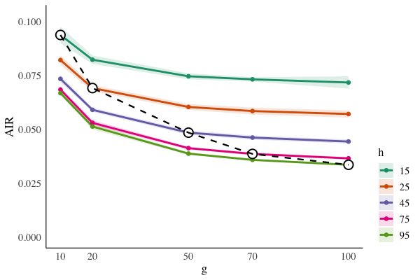
This section assesses the accuracy of the approximations in (10) and (12) to 𝐕−1\mathbf{V}^{-1} under crossed random-effects models with both asymptotic and non-asymptotic unbalanced designs, respectively. Throughout, data are generated from the model in (1), and the variance components are fixed at (σα2,σβ2,σγ2,σe2)=(5,7,3,4)(\sigma_{\alpha}^{2},\sigma_{\beta}^{2},\sigma_{\gamma}^{2},\sigma_{e}^{2})=(5,7,3,4). For each simulation setting, we generate N=200N=200 independent replicates. The two cases below differ only in the grid size (g,h)(g,h) and in how the cell sizes {mi​j}\{m_{ij}\} (and, in Case 2, the truncation order rr) are varied.

Case 1 (Asymptotic setting). We study increasing grids with (g,h)∈{10,20,50,70,100}×{15,25,45,75,95}(g,h)\in\{10,20,50,70,100\}\times\{15,25,45,75,95\}, yielding 25 configurations. For each configuration, the cell sizes are generated as mi​j∼Uniform​(1,15)m_{ij}\sim\mathrm{Uniform}(1,15). This produces 25 simulation settings.

Case 2 (Non-asymptotic setting). We consider relatively small grids with (g,h)∈{10,20}×{15,25}(g,h)\in\{10,20\}\times\{15,25\}. For each configuration, we examine eight levels of unbalance determined by mL∈{10,20}m_{L}\in\{10,20\} and Δ∈{0.15,0.25,0.35,0.45}\Delta\in\{0.15,0.25,0.35,0.45\}, generating cell sizes as mi​j∼Uniform​(mL,mL/(1−Δ))m_{ij}\sim\mathrm{Uniform}(m_{L},\,m_{L}/(1-\Delta)). This yields 32 settings in total. For each replicate in Case 2, the approximation to 𝐕−1\mathbf{V}^{-1} is computed using truncation orders r∈{0,1,2,3,4,5}r\in\{0,1,2,3,4,5\}.

To assess the accuracy of the approximations, we compute the Average Inversion Residual (AIR) for both the estimated 𝐕^−1\hat{\mathbf{V}}^{-1} from (10) and 𝐕^(r)−1\hat{\mathbf{V}}_{(r)}^{-1} from (12), defined as

AIR=1N​∑b=1N1n(b)​‖𝐕(b)​𝐕^−1​(b)−𝐈n(b)‖F,\displaystyle\mathrm{AIR}=\frac{1}{N}\sum_{b=1}^{N}\frac{1}{n^{(b)}}\bigl\|\mathbf{V}^{(b)}\hat{\mathbf{V}}^{-1(b)}-\mathbf{I}_{n^{(b)}}\bigr\|_{F},

where ∥⋅∥F\|\cdot\|_{F} denotes the Frobenius norm, a (b)(b) superscript denotes a quantity related to the bbth independent replicate, 𝐕^−1​(b)\hat{\mathbf{V}}^{-1(b)} represents either 𝐕^−1​(b)\hat{\mathbf{V}}^{-1(b)} or 𝐕^(r)−1​(b)\hat{\mathbf{V}}^{-1(b)}_{(r)} depending on the approximation used, and n(b)n^{(b)} denotes the number of observations in the bbth replicate.

Refer to caption
(a) Case 1: Asymptotic setting
Refer to caption
(b) Case 2: Non-asymptotic setting
Figure 1: Average Inversion Residual (AIR) for both asymptotic and non-asymptotic settings, with shaded areas representing one standard deviation across N=200N=200 replications.

Figure 1 presents the simulation results, where the lines show the mean AIR values and the shaded regions indicate one standard deviation across the replications.

In Figure 1(a), for fixed small hh (e.g., h=15h=15 or 2525), the AIR decreases as gg increases from 10 to 50 and then stabilizes as gg increases further to 100. In contrast, for fixed large hh (e.g., h=75h=75 or 9595), the AIR continues to decrease as gg increases from 10 to 100, with a less pronounced flattening. This pattern arises because the remainder order of each entry in the approximation depends on O​(1/[min⁡(g,h)​mL2])O(1/[\min(g,h)m_{L}^{2}]). Since σe2/(2​mL2​σγ2)<1{\sigma}_{e}^{2}/(2m_{L}^{2}{\sigma}_{\gamma}^{2})<1, Theorem 3 implies ε=0\varepsilon=0. When hh is fixed and small, the remainder order depends primarily on hh, causing the AIR to initially decrease and then level off as gg grows. Conversely, when hh is large, the remainder order depends on gg, resulting in a continued decrease in the AIR. When both gg and hh increase simultaneously (the dashed line with circle markers), min⁡(g,h)\min(g,h) increases and the remainder order becomes smaller, leading to a more pronounced reduction in the AIR. These results are consistent with the theoretical guarantees of Theorem 3.

In Figure 1(b), for fixed gg, hh, mLm_{L}, and Δ\Delta, the AIR decreases monotonically as the truncation order rr increases from 0 to 5, confirming Theorem 4: higher-order approximations yield improved accuracy in estimating the inverse covariance matrix under mildly unbalanced designs. Moreover, holding gg, hh, mLm_{L}, and rr fixed, the AIR decreases as Δ\Delta becomes smaller, indicating that the approximation improves as the design becomes more balanced. This trend is again consistent with the theoretical results established in Theorem 4. The full simulation results are in the Supplementary Material.

5 Discussion

This paper develops a unified and tractable framework for approximating and analyzing the inverse of the covariance matrix in linear mixed models with crossed random effects under unbalanced designs. A modified covariance matrix is introduced whose inverse admits an exact spectral decomposition, providing an elegant and accurate approximation to the true inverse in asymptotic unbalanced settings. For non-asymptotic designs, the inverse of the modified matrix also provides a close analytical approximation under mildly unbalanced data, similar to that in the balanced case. For severely unbalanced data, the exact inverse can be constructed through a sequence of rank-one updates to the modified matrix inverse, offering a computationally feasible alternative to direct inversion. These results support both theoretical developments and scalable inference in settings where standard methods become intractable.

A key innovation of our approach lies in the introduction of the Khatri–Rao product to model covariance structures under unbalanced designs. While Kronecker products have long served as a foundational tool in balanced crossed designs, their utility diminishes when replication varies across cells. The Khatri–Rao product enables a structured yet flexible formulation that accommodates cell-specific replication, and preserves key algebraic properties that facilitate matrix decomposition, inversion, and asymptotic analysis. To our knowledge, this is the first application of the Khatri–Rao product to such models, and it opens new possibilities for modelling and computation in a wide range of applications involving unbalanced data. A promising direction for future work is to extend the asymptotic theory of likelihood-based estimators and predictions to settings with bounded unbalanced cell sizes, building on the approximations and recursive structures established here. In principle, our approach can also extend to more general models, such as kk-way crossed random-effects models with unbalanced designs (k>2k>2).

Appendix A Proofs

The proofs of Theorems and Corollaries are presented in this section. The supporting lemmas used in these proofs are proved in Sections B.

A.1 Proof of Theorem 1

Proof.

Dividing the modified covariance matrix 𝐕ˇ\check{\mathbf{V}} by the corresponding cell size over the maximum cell size, we have

mU​𝐈~𝐦​𝐕ˇ​𝐈~𝐦\displaystyle m_{U}\tilde{\mathbf{I}}_{\mathbf{m}}\check{\mathbf{V}}\tilde{\mathbf{I}}_{\mathbf{m}} =σe2​𝐈n+mU​σα2​(𝐈g⊗𝐉h)cell⊛𝐉~𝐦+mU​σβ2​(𝐉g⊗𝐈h)cell⊛𝐉~𝐦\displaystyle={\sigma}_{e}^{2}\mathbf{I}_{n}+m_{U}\sigma_{\alpha}^{2}(\mathbf{I}_{g}\otimes\mathbf{J}_{h})_{\text{cell}}\circledast\tilde{\mathbf{J}}_{\mathbf{m}}+m_{U}\sigma_{\beta}^{2}(\mathbf{J}_{g}\otimes\mathbf{I}_{h})_{\text{cell}}\circledast\tilde{\mathbf{J}}_{\mathbf{m}}
+mU​σγ2​(𝐈g⊗𝐈h)cell⊛𝐉~𝐦.\displaystyle\qquad+m_{U}\sigma_{\gamma}^{2}(\mathbf{I}_{g}\otimes\mathbf{I}_{h})_{\text{cell}}\circledast\tilde{\mathbf{J}}_{\mathbf{m}}. (14)

The weighted modified covariance matrix of the random effects mU​𝐈~𝐦​𝐕ˇ​𝐈~𝐦m_{U}\tilde{\mathbf{I}}_{\mathbf{m}}\check{\mathbf{V}}\tilde{\mathbf{I}}_{\mathbf{m}} has four terms: one in 𝐈n\mathbf{I}_{n}, one in (𝐈g⊗𝐉h)cell⊛𝐉~𝐦(\mathbf{I}_{g}\otimes\mathbf{J}_{h})_{\text{cell}}\circledast\tilde{\mathbf{J}}_{\mathbf{m}}, one in (𝐉g⊗𝐈h)cell⊛𝐉~𝐦(\mathbf{J}_{g}\otimes\mathbf{I}_{h})_{\text{cell}}\circledast\tilde{\mathbf{J}}_{\mathbf{m}}, and one in (𝐈g⊗𝐈h)cell⊛𝐉~𝐦(\mathbf{I}_{g}\otimes\mathbf{I}_{h})_{\text{cell}}\circledast\tilde{\mathbf{J}}_{\mathbf{m}}. It is therefore clear that any vector which eliminates (𝐈g⊗𝐉h)cell⊛𝐉~𝐦(\mathbf{I}_{g}\otimes\mathbf{J}_{h})_{\text{cell}}\circledast\tilde{\mathbf{J}}_{\mathbf{m}}, (𝐉g⊗𝐈h)cell⊛𝐉~𝐦(\mathbf{J}_{g}\otimes\mathbf{I}_{h})_{\text{cell}}\circledast\tilde{\mathbf{J}}_{\mathbf{m}} and (𝐈g⊗𝐈h)cell⊛𝐉~𝐦(\mathbf{I}_{g}\otimes\mathbf{I}_{h})_{\text{cell}}\circledast\tilde{\mathbf{J}}_{\mathbf{m}} must be a characteristic vector of mU​𝐈~𝐦​𝐕ˇ​𝐈~𝐦m_{U}\tilde{\mathbf{I}}_{\mathbf{m}}\check{\mathbf{V}}\tilde{\mathbf{I}}_{\mathbf{m}} with associated root σe2{\sigma}_{e}^{2}.

We begin by considering vectors of the form (𝝉αi⊗𝝉βj)row⊛𝝉γ,(i,j,k)(\boldsymbol{\tau}_{\alpha_{i}}\otimes\boldsymbol{\tau}_{\beta_{j}})_{\text{row}}\circledast\boldsymbol{\tau}_{\gamma,(i,j,k)}, where 𝝉αi\boldsymbol{\tau}_{\alpha_{i}}, 𝝉βj\boldsymbol{\tau}_{\beta_{j}} and 𝝉γ,(i,j,k)\boldsymbol{\tau}_{\gamma,(i,j,k)} are orthogonal to 𝟏g\boldsymbol{1}_{g}, 𝟏h\boldsymbol{1}_{h}, and 𝟏𝐦\boldsymbol{1}_{\mathbf{m}}, respectively. Since the last three terms in (14) involve 𝐉~𝐦=𝟏~𝐦​𝟏~𝐦⊤\tilde{\mathbf{J}}_{\mathbf{m}}=\tilde{\boldsymbol{1}}_{\mathbf{m}}\tilde{\boldsymbol{1}}_{\mathbf{m}}^{\top}, it follows from Lemma 2 that the last three terms are eliminated by (𝝉αi⊗𝝉βj)row⊛𝝉γ,(i,j,k)(\boldsymbol{\tau}_{\alpha_{i}}\otimes\boldsymbol{\tau}_{\beta_{j}})_{\text{row}}\circledast\boldsymbol{\tau}_{\gamma,(i,j,k)}. These vectors are eigenvectors with eigenvalue σe2{\sigma}_{e}^{2} with multiplicity ∑i=1g−1∑j=1h−1(mi​j−1)\sum_{i=1}^{g-1}\sum_{j=1}^{h-1}(m_{ij}-1).

Similarly, the last three terms are also eliminated by other combinations, such as (𝟏~g⊗𝟏~h)row⊛𝝉γ,(i,j,k)(\tilde{\boldsymbol{1}}_{g}\otimes\tilde{\boldsymbol{1}}_{h})_{\text{row}}\circledast\boldsymbol{\tau}_{\gamma,(i,j,k)}, (𝟏~g⊗𝝉βj)row⊛𝝉γ,(i,j,k)(\tilde{\boldsymbol{1}}_{g}\otimes\boldsymbol{\tau}_{\beta_{j}})_{\text{row}}\circledast\boldsymbol{\tau}_{\gamma,(i,j,k)} and (𝝉αi⊗𝟏~h)row⊛𝝉γ,(i,j,k)(\boldsymbol{\tau}_{\alpha_{i}}\otimes\tilde{\boldsymbol{1}}_{h})_{\text{row}}\circledast\boldsymbol{\tau}_{\gamma,(i,j,k)}, because these combinations all include a common component 𝝉γ,(i,j,k)\boldsymbol{\tau}_{\gamma,(i,j,k)}. These vectors are likewise eigenvectors of mU​𝐈~𝐦​𝐕ˇ​𝐈~𝐦m_{U}\tilde{\mathbf{I}}_{\mathbf{m}}\check{\mathbf{V}}\tilde{\mathbf{I}}_{\mathbf{m}} with eigenvalue σe2{\sigma}_{e}^{2}, and with multiplicities mg​h−1m_{gh}-1, ∑j=1h−1(mg​j−1)\sum_{j=1}^{h-1}(m_{gj}-1), and ∑i=1g−1(mi​h−1)\sum_{i=1}^{g-1}(m_{ih}-1), respectively.

Next, we examine vectors of the form (𝝉αi⊗𝝉βj)row⊛𝟏~𝐦(\boldsymbol{\tau}_{\alpha_{i}}\otimes\boldsymbol{\tau}_{\beta_{j}})_{\text{row}}\circledast\tilde{\boldsymbol{1}}_{\mathbf{m}}, where 𝝉αi\boldsymbol{\tau}_{\alpha_{i}} and 𝝉βj\boldsymbol{\tau}_{\beta_{j}} are orthogonal to 𝟏g\boldsymbol{1}_{g} and 𝟏h\boldsymbol{1}_{h}, respectively. It follows from Lemma 2 that the σα2\sigma_{\alpha}^{2} and σβ2\sigma_{\beta}^{2} terms (involving 𝐉~g=𝟏~g​𝟏~g⊤\tilde{\mathbf{J}}_{g}=\tilde{\boldsymbol{1}}_{g}\tilde{\boldsymbol{1}}_{g}^{\top} and 𝐉~h=𝟏~h​𝟏~h⊤\tilde{\mathbf{J}}_{h}=\tilde{\boldsymbol{1}}_{h}\tilde{\boldsymbol{1}}_{h}^{\top}) vanish, while the σγ2{\sigma}_{\gamma}^{2} term remains active due to its alignment with 𝟏𝐦\boldsymbol{1}_{\mathbf{m}}, as indicated by Lemma 1. Therefore, these vectors are eigenvectors with eigenvalue σe2+mU​σγ2{\sigma}_{e}^{2}+m_{U}\sigma_{\gamma}^{2}, with total multiplicity (g−1)​(h−1)(g-1)(h-1).

Similarly, consider the vectors (𝝉αi⊗𝟏~h)row⊛𝟏~𝐦(\boldsymbol{\tau}_{\alpha_{i}}\otimes\tilde{\boldsymbol{1}}_{h})_{\text{row}}\circledast\tilde{\boldsymbol{1}}_{\mathbf{m}}, where 𝝉αi\boldsymbol{\tau}_{\alpha_{i}} is orthogonal to 𝟏g\boldsymbol{1}_{g}, eliminating the σβ2\sigma_{\beta}^{2} term (involving 𝐉~g=𝟏~g​𝟏~g⊤\tilde{\mathbf{J}}_{g}=\tilde{\boldsymbol{1}}_{g}\tilde{\boldsymbol{1}}_{g}^{\top}). The σα2{\sigma}_{\alpha}^{2} and σγ2{\sigma}_{\gamma}^{2} terms are aligned with their corresponding projection directions, so the σα2\sigma_{\alpha}^{2} and σγ2\sigma_{\gamma}^{2} terms remain. According to Lemma 1 and 2, the eigenvalue associated with these vectors is σe2+mU​σγ2+h​mU​σα2{\sigma}_{e}^{2}+m_{U}\sigma_{\gamma}^{2}+hm_{U}\sigma_{\alpha}^{2}, and the multiplicity is g−1g-1. Likewise, vectors of the form (𝟏~g⊗𝝉βj)row⊛𝟏~𝐦(\tilde{\boldsymbol{1}}_{g}\otimes\boldsymbol{\tau}_{\beta_{j}})_{\text{row}}\circledast\tilde{\boldsymbol{1}}_{\mathbf{m}} yield eigenvalue σe2+mU​σγ2+g​mU​σβ2{\sigma}_{e}^{2}+m_{U}\sigma_{\gamma}^{2}+gm_{U}\sigma_{\beta}^{2}. Since 𝝉βj\boldsymbol{\tau}_{\beta_{j}} is orthogonal to 𝟏h\boldsymbol{1}_{h}, the σα2\sigma_{\alpha}^{2} term (involving 𝐉~h=𝟏~h​𝟏~h⊤\tilde{\mathbf{J}}_{h}=\tilde{\boldsymbol{1}}_{h}\tilde{\boldsymbol{1}}_{h}^{\top}) vanishes, while the σβ2{\sigma}_{\beta}^{2} and σγ2{\sigma}_{\gamma}^{2} terms are preserved by the alignment of 𝟏~g\tilde{\boldsymbol{1}}_{g} and 𝟏~𝐦\tilde{\boldsymbol{1}}_{\mathbf{m}}. The multiplicity is h−1h-1.

Finally, the fully aligned direction (𝟏~g⊗𝟏~h)row⊛𝟏~𝐦(\tilde{\boldsymbol{1}}_{g}\otimes\tilde{\boldsymbol{1}}_{h})_{\text{row}}\circledast\tilde{\boldsymbol{1}}_{\mathbf{m}} lies within the span of all four projection directions. Consequently, all terms in (14) contribute to the eigenvalue, and by Lemma 1 and 2, the resulting eigenvalue is σe2+mU​σγ2+h​mU​σα2+g​mU​σβ2{\sigma}_{e}^{2}+m_{U}\sigma_{\gamma}^{2}+hm_{U}\sigma_{\alpha}^{2}+gm_{U}\sigma_{\beta}^{2}, with multiplicity one.

∎

A.2 Proof of Corollary 2

Proof.

We have mU​𝐈~𝐦​𝐕ˇ​𝐈~𝐦=𝐂⊤​𝚲λ​𝐂m_{U}\tilde{\mathbf{I}}_{\mathbf{m}}\check{\mathbf{V}}\tilde{\mathbf{I}}_{\mathbf{m}}=\mathbf{C}^{\top}\boldsymbol{\Lambda}_{\lambda}\mathbf{C} and 𝐂⊤​𝐂=𝐈\mathbf{C}^{\top}\mathbf{C}=\mathbf{I} following Theorem 1. The inverse is

(mU​𝐈~𝐦​𝐕ˇ​𝐈~𝐦)−1=𝐂⊤​𝚲1/λ​𝐂,\displaystyle(m_{U}\tilde{\mathbf{I}}_{\mathbf{m}}\check{\mathbf{V}}\tilde{\mathbf{I}}_{\mathbf{m}})^{-1}=\mathbf{C}^{\top}\boldsymbol{\Lambda}_{1/\lambda}\mathbf{C},

where

𝚲1/λ\displaystyle\boldsymbol{\Lambda}_{1/\lambda}
=diag[1/λ1, 1/λ0𝐈[mg​h−1:mg​h−1], 1/λ3𝐈h−1, 1/λ0𝐈[∑j=1h−1(mg​j−1):∑j=1h−1(mg​j−1)], 1/λ5𝐈g−1,\displaystyle=\operatorname{diag}\bigl[1/\lambda_{1},\,1/\lambda_{0}\mathbf{I}_{[m_{gh}-1:m_{gh}-1]},\,1/\lambda_{3}\mathbf{I}_{h-1},\,1/\lambda_{0}\mathbf{I}_{[\sum_{j=1}^{h-1}(m_{gj}-1):\sum_{j=1}^{h-1}(m_{gj}-1)]},\,1/\lambda_{5}\mathbf{I}_{g-1},
1/λ0𝐈[∑i=1g−1(mi​h−1):∑i=1g−1(mi​h−1)], 1/λ7𝐈(g−1)​(h−1), 1/λ0𝐈[∑i=1g−1∑j=1h−1(mi​j−1):∑i=1g−1∑j=1h−1(mi​j−1)]].\displaystyle\quad 1/\lambda_{0}\mathbf{I}_{[\sum_{i=1}^{g-1}(m_{ih}-1):\sum_{i=1}^{g-1}(m_{ih}-1)]},\,1/\lambda_{7}\mathbf{I}_{(g-1)(h-1)},\,1/\lambda_{0}\mathbf{I}_{[\sum_{i=1}^{g-1}\sum_{j=1}^{h-1}(m_{ij}-1):\sum_{i=1}^{g-1}\sum_{j=1}^{h-1}(m_{ij}-1)]}\bigr].

Thus

(mU​𝐈~𝐦​𝐕ˇ​𝐈~𝐦)−1=𝐂⊤​𝚲1/λ​𝐂=\displaystyle(m_{U}\tilde{\mathbf{I}}_{\mathbf{m}}\check{\mathbf{V}}\tilde{\mathbf{I}}_{\mathbf{m}})^{-1}=\mathbf{C}^{\top}\boldsymbol{\Lambda}_{1/\lambda}\mathbf{C}= 1λ1​𝐂1​𝐂1⊤+1λ3​𝐂3​𝐂3⊤+1λ5​𝐂5​𝐂5⊤+1λ7​𝐂7​𝐂7⊤\displaystyle\frac{1}{\lambda_{1}}\mathbf{C}_{1}\mathbf{C}_{1}^{\top}+\frac{1}{\lambda_{3}}\mathbf{C}_{3}\mathbf{C}_{3}^{\top}+\frac{1}{\lambda_{5}}\mathbf{C}_{5}\mathbf{C}_{5}^{\top}+\frac{1}{\lambda_{7}}\mathbf{C}_{7}\mathbf{C}_{7}^{\top}
+1λ0​(𝐂2​𝐂2⊤+𝐂4​𝐂4⊤+𝐂6​𝐂6⊤+𝐂8​𝐂8⊤).\displaystyle+\frac{1}{\lambda_{0}}(\mathbf{C}_{2}\mathbf{C}_{2}^{\top}+\mathbf{C}_{4}\mathbf{C}_{4}^{\top}+\mathbf{C}_{6}\mathbf{C}_{6}^{\top}+\mathbf{C}_{8}\mathbf{C}_{8}^{\top}).

We have

𝐂1​𝐂1⊤\displaystyle\mathbf{C}_{1}\mathbf{C}_{1}^{\top} =[(𝟏~g⊗𝟏~h)row⊛𝟏~𝐦]​[(𝟏~g⊗𝟏~h)row⊛𝟏~𝐦]⊤=(𝐉~g⊗𝐉~h)cell⊛𝐉~𝐦.\displaystyle=[(\tilde{\boldsymbol{1}}_{g}\otimes\tilde{\boldsymbol{1}}_{h})_{\text{row}}\circledast\tilde{\boldsymbol{1}}_{\mathbf{m}}][(\tilde{\boldsymbol{1}}_{g}\otimes\tilde{\boldsymbol{1}}_{h})_{\text{row}}\circledast\tilde{\boldsymbol{1}}_{\mathbf{m}}]^{\top}=(\tilde{\mathbf{J}}_{g}\otimes\tilde{\mathbf{J}}_{h})_{\text{cell}}\circledast\tilde{\mathbf{J}}_{\mathbf{m}}. (15)

Now, consider the product

𝐂⊤​𝐂=𝐂1​𝐂1⊤+𝐂2​𝐂2⊤+𝐂3​𝐂3⊤+𝐂4​𝐂4⊤+𝐂5​𝐂5⊤+𝐂6​𝐂6⊤+𝐂7​𝐂7⊤+𝐂8​𝐂8⊤=𝐈n.\displaystyle\mathbf{C}^{\top}\mathbf{C}=\mathbf{C}_{1}\mathbf{C}_{1}^{\top}+\mathbf{C}_{2}\mathbf{C}_{2}^{\top}+\mathbf{C}_{3}\mathbf{C}_{3}^{\top}+\mathbf{C}_{4}\mathbf{C}_{4}^{\top}+\mathbf{C}_{5}\mathbf{C}_{5}^{\top}+\mathbf{C}_{6}\mathbf{C}_{6}^{\top}+\mathbf{C}_{7}\mathbf{C}_{7}^{\top}+\mathbf{C}_{8}\mathbf{C}_{8}^{\top}=\mathbf{I}_{n}. (16)

Premultiplying (16) by (𝐉g⊗𝐈h)cell⊛𝐉~𝐦(\mathbf{J}_{g}\otimes\mathbf{I}_{h})_{\text{cell}}\circledast\tilde{\mathbf{J}}_{\mathbf{m}} and following Lemma 1, we have

[(𝐉g⊗𝐈h)cell⊛𝐉~𝐦]​𝐂1​𝐂1⊤=g​𝐂1​𝐂1⊤=g​(𝐉~g⊗𝐉~h)cell⊛𝐉~𝐦,\displaystyle[(\mathbf{J}_{g}\otimes\mathbf{I}_{h})_{\text{cell}}\circledast\tilde{\mathbf{J}}_{\mathbf{m}}]\mathbf{C}_{1}\mathbf{C}_{1}^{\top}=g\mathbf{C}_{1}\mathbf{C}_{1}^{\top}=g(\tilde{\mathbf{J}}_{g}\otimes\tilde{\mathbf{J}}_{h})_{\text{cell}}\circledast\tilde{\mathbf{J}}_{\mathbf{m}}, [(𝐉g⊗𝐈h)cell⊛𝐉~𝐦]​𝐂2​𝐂2⊤=𝟎[n:n],\displaystyle[(\mathbf{J}_{g}\otimes\mathbf{I}_{h})_{\text{cell}}\circledast\tilde{\mathbf{J}}_{\mathbf{m}}]\mathbf{C}_{2}\mathbf{C}_{2}^{\top}=\boldsymbol{0}_{[n:n]},
[(𝐉g⊗𝐈h)cell⊛𝐉~𝐦]​𝐂3​𝐂3⊤=g​𝐂3​𝐂3⊤,\displaystyle[(\mathbf{J}_{g}\otimes\mathbf{I}_{h})_{\text{cell}}\circledast\tilde{\mathbf{J}}_{\mathbf{m}}]\mathbf{C}_{3}\mathbf{C}_{3}^{\top}=g\mathbf{C}_{3}\mathbf{C}_{3}^{\top}, [(𝐉g⊗𝐈h)cell⊛𝐉~𝐦]​𝐂4​𝐂4⊤=𝟎[n:n],\displaystyle[(\mathbf{J}_{g}\otimes\mathbf{I}_{h})_{\text{cell}}\circledast\tilde{\mathbf{J}}_{\mathbf{m}}]\mathbf{C}_{4}\mathbf{C}_{4}^{\top}=\boldsymbol{0}_{[n:n]},
[(𝐉g⊗𝐈h)cell⊛𝐉~𝐦]​𝐂5​𝐂5⊤=𝟎[n:n],\displaystyle[(\mathbf{J}_{g}\otimes\mathbf{I}_{h})_{\text{cell}}\circledast\tilde{\mathbf{J}}_{\mathbf{m}}]\mathbf{C}_{5}\mathbf{C}_{5}^{\top}=\boldsymbol{0}_{[n:n]}, [(𝐉g⊗𝐈h)cell⊛𝐉~𝐦]​𝐂6​𝐂6⊤=𝟎[n:n],\displaystyle[(\mathbf{J}_{g}\otimes\mathbf{I}_{h})_{\text{cell}}\circledast\tilde{\mathbf{J}}_{\mathbf{m}}]\mathbf{C}_{6}\mathbf{C}_{6}^{\top}=\boldsymbol{0}_{[n:n]},
[(𝐉g⊗𝐈h)cell⊛𝐉~𝐦]​𝐂7​𝐂7⊤=𝟎[n:n],\displaystyle[(\mathbf{J}_{g}\otimes\mathbf{I}_{h})_{\text{cell}}\circledast\tilde{\mathbf{J}}_{\mathbf{m}}]\mathbf{C}_{7}\mathbf{C}_{7}^{\top}=\boldsymbol{0}_{[n:n]}, [(𝐉g⊗𝐈h)cell⊛𝐉~𝐦]​𝐂8​𝐂8⊤=𝟎[n:n].\displaystyle[(\mathbf{J}_{g}\otimes\mathbf{I}_{h})_{\text{cell}}\circledast\tilde{\mathbf{J}}_{\mathbf{m}}]\mathbf{C}_{8}\mathbf{C}_{8}^{\top}=\boldsymbol{0}_{[n:n]}.

It then follows that

𝐂3​𝐂3⊤=(𝐉~g⊗𝐈h)cell⊛𝐉~𝐦−(𝐉~g⊗𝐉~h)cell⊛𝐉~𝐦=[𝐉~g⊗(𝐈h−𝐉~h)]cell⊛𝐉~𝐦.\displaystyle\mathbf{C}_{3}\mathbf{C}_{3}^{\top}=(\tilde{\mathbf{J}}_{g}\otimes\mathbf{I}_{h})_{\text{cell}}\circledast\tilde{\mathbf{J}}_{\mathbf{m}}-(\tilde{\mathbf{J}}_{g}\otimes\tilde{\mathbf{J}}_{h})_{\text{cell}}\circledast\tilde{\mathbf{J}}_{\mathbf{m}}=\left[\tilde{\mathbf{J}}_{g}\otimes(\mathbf{I}_{h}-\tilde{\mathbf{J}}_{h})\right]_{\text{cell}}\circledast\tilde{\mathbf{J}}_{\mathbf{m}}. (17)

Similarly, premultiplying (16) by (𝐈g⊗𝐉h)cell⊛𝐉~𝐦(\mathbf{I}_{g}\otimes\mathbf{J}_{h})_{\text{cell}}\circledast\tilde{\mathbf{J}}_{\mathbf{m}} and following Lemma 1, we have

[(𝐈g⊗𝐉h)cell⊛𝐉~𝐦]​𝐂1​𝐂1⊤=h​𝐂1​𝐂1⊤=h​(𝐉~g⊗𝐉~h)cell⊛𝐉~𝐦,\displaystyle[(\mathbf{I}_{g}\otimes\mathbf{J}_{h})_{\text{cell}}\circledast\tilde{\mathbf{J}}_{\mathbf{m}}]\mathbf{C}_{1}\mathbf{C}_{1}^{\top}=h\mathbf{C}_{1}\mathbf{C}_{1}^{\top}=h(\tilde{\mathbf{J}}_{g}\otimes\tilde{\mathbf{J}}_{h})_{\text{cell}}\circledast\tilde{\mathbf{J}}_{\mathbf{m}}, [(𝐈g⊗𝐉h)cell⊛𝐉~𝐦]​𝐂2​𝐂2⊤=𝟎[n:n],\displaystyle[(\mathbf{I}_{g}\otimes\mathbf{J}_{h})_{\text{cell}}\circledast\tilde{\mathbf{J}}_{\mathbf{m}}]\mathbf{C}_{2}\mathbf{C}_{2}^{\top}=\boldsymbol{0}_{[n:n]},
[(𝐈g⊗𝐉h)cell⊛𝐉~𝐦]​𝐂3​𝐂3⊤=𝟎[n:n],\displaystyle[(\mathbf{I}_{g}\otimes\mathbf{J}_{h})_{\text{cell}}\circledast\tilde{\mathbf{J}}_{\mathbf{m}}]\mathbf{C}_{3}\mathbf{C}_{3}^{\top}=\boldsymbol{0}_{[n:n]}, [(𝐈g⊗𝐉h)cell⊛𝐉~𝐦]​𝐂4​𝐂4⊤=𝟎[n:n],\displaystyle[(\mathbf{I}_{g}\otimes\mathbf{J}_{h})_{\text{cell}}\circledast\tilde{\mathbf{J}}_{\mathbf{m}}]\mathbf{C}_{4}\mathbf{C}_{4}^{\top}=\boldsymbol{0}_{[n:n]},
[(𝐈g⊗𝐉h)cell⊛𝐉~𝐦]​𝐂5​𝐂5⊤=h​𝐂5​𝐂5⊤,\displaystyle[(\mathbf{I}_{g}\otimes\mathbf{J}_{h})_{\text{cell}}\circledast\tilde{\mathbf{J}}_{\mathbf{m}}]\mathbf{C}_{5}\mathbf{C}_{5}^{\top}=h\mathbf{C}_{5}\mathbf{C}_{5}^{\top}, [(𝐈g⊗𝐉h)cell⊛𝐉~𝐦]​𝐂6​𝐂6⊤=𝟎[n:n],\displaystyle[(\mathbf{I}_{g}\otimes\mathbf{J}_{h})_{\text{cell}}\circledast\tilde{\mathbf{J}}_{\mathbf{m}}]\mathbf{C}_{6}\mathbf{C}_{6}^{\top}=\boldsymbol{0}_{[n:n]},
[(𝐈g⊗𝐉h)cell⊛𝐉~𝐦]​𝐂7​𝐂7⊤=𝟎[n:n],\displaystyle[(\mathbf{I}_{g}\otimes\mathbf{J}_{h})_{\text{cell}}\circledast\tilde{\mathbf{J}}_{\mathbf{m}}]\mathbf{C}_{7}\mathbf{C}_{7}^{\top}=\boldsymbol{0}_{[n:n]}, [(𝐈g⊗𝐉h)cell⊛𝐉~𝐦]​𝐂8​𝐂8⊤=𝟎[n:n].\displaystyle[(\mathbf{I}_{g}\otimes\mathbf{J}_{h})_{\text{cell}}\circledast\tilde{\mathbf{J}}_{\mathbf{m}}]\mathbf{C}_{8}\mathbf{C}_{8}^{\top}=\boldsymbol{0}_{[n:n]}.

It then follows that

𝐂5​𝐂5⊤=(𝐈g⊗𝐉~h)cell⊛𝐉~𝐦−(𝐉~g⊗𝐉~h)cell⊛𝐉~𝐦=[(𝐈g−𝐉~g)⊗𝐉~h]cell⊛𝐉~𝐦.\displaystyle\mathbf{C}_{5}\mathbf{C}_{5}^{\top}=(\mathbf{I}_{g}\otimes\tilde{\mathbf{J}}_{h})_{\text{cell}}\circledast\tilde{\mathbf{J}}_{\mathbf{m}}-(\tilde{\mathbf{J}}_{g}\otimes\tilde{\mathbf{J}}_{h})_{\text{cell}}\circledast\tilde{\mathbf{J}}_{\mathbf{m}}=\left[(\mathbf{I}_{g}-\tilde{\mathbf{J}}_{g})\otimes\tilde{\mathbf{J}}_{h}\right]_{\text{cell}}\circledast\tilde{\mathbf{J}}_{\mathbf{m}}. (18)

In the same manner, premultiplying (16) by (𝐈g⊗𝐈h)cell⊛𝐉~𝐦(\mathbf{I}_{g}\otimes\mathbf{I}_{h})_{\text{cell}}\circledast\tilde{\mathbf{J}}_{\mathbf{m}} and following Lemma 1, we have

[(𝐉g⊗𝐈h)cell⊛𝐉~𝐦]​𝐂1​𝐂1⊤=𝐂1​𝐂1⊤,\displaystyle[(\mathbf{J}_{g}\otimes\mathbf{I}_{h})_{\text{cell}}\circledast\tilde{\mathbf{J}}_{\mathbf{m}}]\mathbf{C}_{1}\mathbf{C}_{1}^{\top}=\mathbf{C}_{1}\mathbf{C}_{1}^{\top}, [(𝐉g⊗𝐈h)cell⊛𝐉~𝐦]​𝐂2​𝐂2⊤=𝟎[n:n],\displaystyle[(\mathbf{J}_{g}\otimes\mathbf{I}_{h})_{\text{cell}}\circledast\tilde{\mathbf{J}}_{\mathbf{m}}]\mathbf{C}_{2}\mathbf{C}_{2}^{\top}=\boldsymbol{0}_{[n:n]},
[(𝐉g⊗𝐈h)cell⊛𝐉~𝐦]​𝐂3​𝐂3⊤=𝐂3​𝐂3⊤,\displaystyle[(\mathbf{J}_{g}\otimes\mathbf{I}_{h})_{\text{cell}}\circledast\tilde{\mathbf{J}}_{\mathbf{m}}]\mathbf{C}_{3}\mathbf{C}_{3}^{\top}=\mathbf{C}_{3}\mathbf{C}_{3}^{\top}, [(𝐉g⊗𝐈h)cell⊛𝐉~𝐦]​𝐂4​𝐂4⊤=𝟎[n:n],\displaystyle[(\mathbf{J}_{g}\otimes\mathbf{I}_{h})_{\text{cell}}\circledast\tilde{\mathbf{J}}_{\mathbf{m}}]\mathbf{C}_{4}\mathbf{C}_{4}^{\top}=\boldsymbol{0}_{[n:n]},
[(𝐉g⊗𝐈h)cell⊛𝐉~𝐦]​𝐂5​𝐂5⊤=𝐂5​𝐂5⊤,\displaystyle[(\mathbf{J}_{g}\otimes\mathbf{I}_{h})_{\text{cell}}\circledast\tilde{\mathbf{J}}_{\mathbf{m}}]\mathbf{C}_{5}\mathbf{C}_{5}^{\top}=\mathbf{C}_{5}\mathbf{C}_{5}^{\top}, [(𝐉g⊗𝐈h)cell⊛𝐉~𝐦]​𝐂6​𝐂6⊤=𝟎[n:n],\displaystyle[(\mathbf{J}_{g}\otimes\mathbf{I}_{h})_{\text{cell}}\circledast\tilde{\mathbf{J}}_{\mathbf{m}}]\mathbf{C}_{6}\mathbf{C}_{6}^{\top}=\boldsymbol{0}_{[n:n]},
[(𝐉g⊗𝐈h)cell⊛𝐉~𝐦]​𝐂7​𝐂7⊤=𝐂7​𝐂7⊤,\displaystyle[(\mathbf{J}_{g}\otimes\mathbf{I}_{h})_{\text{cell}}\circledast\tilde{\mathbf{J}}_{\mathbf{m}}]\mathbf{C}_{7}\mathbf{C}_{7}^{\top}=\mathbf{C}_{7}\mathbf{C}_{7}^{\top}, [(𝐉g⊗𝐈h)cell⊛𝐉~𝐦]​𝐂8​𝐂8⊤=𝟎[n:n].\displaystyle[(\mathbf{J}_{g}\otimes\mathbf{I}_{h})_{\text{cell}}\circledast\tilde{\mathbf{J}}_{\mathbf{m}}]\mathbf{C}_{8}\mathbf{C}_{8}^{\top}=\boldsymbol{0}_{[n:n]}.

Then combining (15), (17) and (18), we have

𝐂7​𝐂7⊤=\displaystyle\mathbf{C}_{7}\mathbf{C}_{7}^{\top}= (𝐈g⊗𝐈h)cell⊛𝐉~𝐦−𝐂1​𝐂1⊤−𝐂3​𝐂3⊤−𝐂5​𝐂5⊤\displaystyle(\mathbf{I}_{g}\otimes\mathbf{I}_{h})_{\text{cell}}\circledast\tilde{\mathbf{J}}_{\mathbf{m}}-\mathbf{C}_{1}\mathbf{C}_{1}^{\top}-\mathbf{C}_{3}\mathbf{C}_{3}^{\top}-\mathbf{C}_{5}\mathbf{C}_{5}^{\top}
=\displaystyle= (𝐈g⊗𝐈h)cell⊛𝐉~𝐦−(𝐉~g⊗𝐉~h)cell⊛𝐉~𝐦\displaystyle(\mathbf{I}_{g}\otimes\mathbf{I}_{h})_{\text{cell}}\circledast\tilde{\mathbf{J}}_{\mathbf{m}}-(\tilde{\mathbf{J}}_{g}\otimes\tilde{\mathbf{J}}_{h})_{\text{cell}}\circledast\tilde{\mathbf{J}}_{\mathbf{m}}
−[𝐉~g⊗(𝐈h−𝐉~h)]cell⊛𝐉~𝐦−[(𝐈g−𝐉~g)⊗𝐉~h]cell⊛𝐉~𝐦\displaystyle-\left[\tilde{\mathbf{J}}_{g}\otimes(\mathbf{I}_{h}-\tilde{\mathbf{J}}_{h})\right]_{\text{cell}}\circledast\tilde{\mathbf{J}}_{\mathbf{m}}-\left[(\mathbf{I}_{g}-\tilde{\mathbf{J}}_{g})\otimes\tilde{\mathbf{J}}_{h}\right]_{\text{cell}}\circledast\tilde{\mathbf{J}}_{\mathbf{m}}
=\displaystyle= [(𝐈g−𝐉~g)⊗(𝐈h−𝐉~h)]cell⊛𝐉~𝐦.\displaystyle\left[(\mathbf{I}_{g}-\tilde{\mathbf{J}}_{g})\otimes(\mathbf{I}_{h}-\tilde{\mathbf{J}}_{h})\right]_{\text{cell}}\circledast\tilde{\mathbf{J}}_{\mathbf{m}}. (19)

Hence

𝐂2​𝐂2⊤+𝐂4​𝐂4⊤+𝐂6​𝐂6⊤+𝐂8​𝐂8⊤\displaystyle\mathbf{C}_{2}\mathbf{C}_{2}^{\top}+\mathbf{C}_{4}\mathbf{C}_{4}^{\top}+\mathbf{C}_{6}\mathbf{C}_{6}^{\top}+\mathbf{C}_{8}\mathbf{C}_{8}^{\top} =𝐈n−𝐂1​𝐂1⊤−𝐂3​𝐂3⊤−𝐂5​𝐂5⊤−𝐂7​𝐂7⊤\displaystyle=\mathbf{I}_{n}-\mathbf{C}_{1}\mathbf{C}_{1}^{\top}-\mathbf{C}_{3}\mathbf{C}_{3}^{\top}-\mathbf{C}_{5}\mathbf{C}_{5}^{\top}-\mathbf{C}_{7}\mathbf{C}_{7}^{\top}
=𝐈n−(𝐈g⊗𝐈h)cell⊛𝐉~𝐦\displaystyle=\mathbf{I}_{n}-(\mathbf{I}_{g}\otimes\mathbf{I}_{h})_{\text{cell}}\circledast\tilde{\mathbf{J}}_{\mathbf{m}}
=(𝐈g⊗𝐈h)cell⊛(𝐈𝐦−𝐉~𝐦).\displaystyle=(\mathbf{I}_{g}\otimes\mathbf{I}_{h})_{\text{cell}}\circledast(\mathbf{I}_{\mathbf{m}}-\tilde{\mathbf{J}}_{\mathbf{m}}). (20)

It follows that an explicit representation of (mU​𝐈~𝐦​𝐕ˇ​𝐈~𝐦)−1(m_{U}\tilde{\mathbf{I}}_{\mathbf{m}}\check{\mathbf{V}}\tilde{\mathbf{I}}_{\mathbf{m}})^{-1} is then

(mU​𝐈~𝐦​𝐕ˇ​𝐈~𝐦)−1=\displaystyle(m_{U}\tilde{\mathbf{I}}_{\mathbf{m}}\check{\mathbf{V}}\tilde{\mathbf{I}}_{\mathbf{m}})^{-1}= 1λ1​(𝐉~g⊗𝐉~h)cell⊛𝐉~𝐦+1λ3​[𝐉~g⊗(𝐈h−𝐉~h)]cell⊛𝐉~𝐦\displaystyle\frac{1}{\lambda_{1}}(\tilde{\mathbf{J}}_{g}\otimes\tilde{\mathbf{J}}_{h})_{\text{cell}}\circledast\tilde{\mathbf{J}}_{\mathbf{m}}+\frac{1}{\lambda_{3}}\left[\tilde{\mathbf{J}}_{g}\otimes(\mathbf{I}_{h}-\tilde{\mathbf{J}}_{h})\right]_{\text{cell}}\circledast\tilde{\mathbf{J}}_{\mathbf{m}}
+1λ5​[(𝐈g−𝐉~g)⊗𝐉~h]cell⊛𝐉~𝐦+1λ7​[(𝐈g−𝐉~g)⊗(𝐈h−𝐉~h)]cell⊛𝐉~𝐦\displaystyle+\frac{1}{\lambda_{5}}\left[(\mathbf{I}_{g}-\tilde{\mathbf{J}}_{g})\otimes\tilde{\mathbf{J}}_{h}\right]_{\text{cell}}\circledast\tilde{\mathbf{J}}_{\mathbf{m}}+\frac{1}{\lambda_{7}}\left[(\mathbf{I}_{g}-\tilde{\mathbf{J}}_{g})\otimes(\mathbf{I}_{h}-\tilde{\mathbf{J}}_{h})\right]_{\text{cell}}\circledast\tilde{\mathbf{J}}_{\mathbf{m}}
+1λ0​[𝐈n−(𝐈g⊗𝐈h)cell⊛𝐉~𝐦].\displaystyle+\frac{1}{\lambda_{0}}\left[\mathbf{I}_{n}-(\mathbf{I}_{g}\otimes\mathbf{I}_{h})_{\text{cell}}\circledast\tilde{\mathbf{J}}_{\mathbf{m}}\right]. (21)

Let 𝐉~a0=𝐈a\tilde{\mathbf{J}}_{a}^{0}=\mathbf{I}_{a}, 𝐉~a1=𝐉~a\tilde{\mathbf{J}}_{a}^{1}=\tilde{\mathbf{J}}_{a}, and

δ00=1λ7−1λ0,δ01=1λ5−1λ7,δ10=1λ3−1λ7,δ11=1λ1−1λ3−1λ5+1λ7.\displaystyle\delta_{00}=\frac{1}{\lambda_{7}}-\frac{1}{\lambda_{0}},\quad\delta_{01}=\frac{1}{\lambda_{5}}-\frac{1}{\lambda_{7}},\quad\delta_{10}=\frac{1}{\lambda_{3}}-\frac{1}{\lambda_{7}},\quad\delta_{11}=\frac{1}{\lambda_{1}}-\frac{1}{\lambda_{3}}-\frac{1}{\lambda_{5}}+\frac{1}{\lambda_{7}}.

We can rewrite

(mU​𝐈~𝐦​𝐕ˇ​𝐈~𝐦)−1=1λ0​𝐈n+[∑𝐢=𝟎𝟏δi1​i2​(𝐉~gi1⊗𝐉~hi2)]cell⊛𝐉~𝐦,\displaystyle(m_{U}\tilde{\mathbf{I}}_{\mathbf{m}}\check{\mathbf{V}}\tilde{\mathbf{I}}_{\mathbf{m}})^{-1}=\frac{1}{\lambda_{0}}\mathbf{I}_{n}+[\sum_{\mathbf{i}=\boldsymbol{0}}^{\boldsymbol{1}}\delta_{i_{1}i_{2}}(\tilde{\mathbf{J}}_{g}^{i_{1}}\otimes\tilde{\mathbf{J}}_{h}^{i_{2}})]_{\text{cell}}\circledast\tilde{\mathbf{J}}_{\mathbf{m}},

where the exponents, i1i_{1} and i2i_{2} are also used as subscripts to δ\delta for notational convenience and readability. They are treated as components of the binary vector 𝐢\mathbf{i}, with the subscripts written in reverse natural order to allow interpretation of 𝐢\mathbf{i} as binary numbers. The summation ∑𝐢=𝟎𝟏\sum_{\mathbf{i}=\boldsymbol{0}}^{\boldsymbol{1}} denotes the sum over the 44 binary vectors from 00 to 11.

Following Lemma 1, we then have

𝐕ˇ−1\displaystyle\check{\mathbf{V}}^{-1} =mUλ0​𝐈¯𝐦+mU​𝐈~𝐦​{[∑𝐢=𝟎𝟏δi1​i2​(𝐉~gi1⊗𝐉~hi2)]cell⊛𝐉~𝐦}​𝐈~𝐦\displaystyle=\frac{m_{U}}{\lambda_{0}}\bar{\mathbf{I}}_{\mathbf{m}}+m_{U}\tilde{\mathbf{I}}_{\mathbf{m}}\{[\sum_{\mathbf{i}=\boldsymbol{0}}^{\boldsymbol{1}}\delta_{i_{1}i_{2}}(\tilde{\mathbf{J}}_{g}^{i_{1}}\otimes\tilde{\mathbf{J}}_{h}^{i_{2}})]_{\text{cell}}\circledast\tilde{\mathbf{J}}_{\mathbf{m}}\}\tilde{\mathbf{I}}_{\mathbf{m}}
=mUλ0​𝐈¯𝐦+mU​[∑𝐢=𝟎𝟏δi1​i2​(𝐉~gi1⊗𝐉~hi2)]cell⊛𝐉¯𝐦.\displaystyle=\frac{m_{U}}{\lambda_{0}}\bar{\mathbf{I}}_{\mathbf{m}}+m_{U}[\sum_{\mathbf{i}=\boldsymbol{0}}^{\boldsymbol{1}}\delta_{i_{1}i_{2}}(\tilde{\mathbf{J}}_{g}^{i_{1}}\otimes\tilde{\mathbf{J}}_{h}^{i_{2}})]_{\text{cell}}\circledast\bar{\mathbf{J}}_{\mathbf{m}}.

∎

A.3 Proof of Theorem 3

Proof.

We write

𝐕=𝐕ˇ+σe2​𝐈n−σe2mU​𝐈𝐦M=𝐕ˇ+σe2​𝐈𝐦Δ,\displaystyle\mathbf{V}=\check{\mathbf{V}}+{\sigma}_{e}^{2}\mathbf{I}_{n}-\frac{{\sigma}_{e}^{2}}{m_{U}}\mathbf{I}_{\mathbf{m}}^{M}=\check{\mathbf{V}}+{\sigma}_{e}^{2}\mathbf{I}_{\mathbf{m}}^{\Delta},

where 𝐈𝐦Δ=diag⁡[(1−mi​j/mU)​𝐈mi​j]\mathbf{I}_{\mathbf{m}}^{\Delta}=\operatorname{diag}[(1-m_{ij}/m_{U})\mathbf{I}_{m_{ij}}]. Following the Woodbury matrix identity, we have

𝐕−1=(𝐕ˇ+σe2​𝐈𝐦Δ)−1=𝐕ˇ−1−𝐕ˇ−1​(1σe2​𝐈𝐦Δ−1+𝐕ˇ−1)−1​𝐕ˇ−1.\displaystyle\mathbf{V}^{-1}=(\check{\mathbf{V}}+{\sigma}_{e}^{2}\mathbf{I}_{\mathbf{m}}^{\Delta})^{-1}=\check{\mathbf{V}}^{-1}-\check{\mathbf{V}}^{-1}\Bigl(\frac{1}{{\sigma}_{e}^{2}}\mathbf{I}_{\mathbf{m}}^{\Delta-1}+\check{\mathbf{V}}^{-1}\Bigr)^{-1}\check{\mathbf{V}}^{-1}.

Recalling Corollary 2, we rewrite (7) as

𝐕ˇ−1=\displaystyle\check{\mathbf{V}}^{-1}= mUλ0​𝐈¯𝐦+mU​(1λ7−1λ0)​(𝐈g⊗𝐈h)cell⊛𝐉¯𝐦+mU​(1λ5−1λ7)​(𝐉~g⊗𝐈h)cell⊛𝐉¯𝐦\displaystyle\frac{m_{U}}{\lambda_{0}}\bar{\mathbf{I}}_{\mathbf{m}}+m_{U}\Bigl(\frac{1}{\lambda_{7}}-\frac{1}{\lambda_{0}}\Bigr)(\mathbf{I}_{g}\otimes\mathbf{I}_{h})_{\text{cell}}\circledast\bar{\mathbf{J}}_{\mathbf{m}}+m_{U}\Bigl(\frac{1}{\lambda_{5}}-\frac{1}{\lambda_{7}}\Bigr)(\tilde{\mathbf{J}}_{g}\otimes\mathbf{I}_{h})_{\text{cell}}\circledast\bar{\mathbf{J}}_{\mathbf{m}}
+mU​(1λ3−1λ7)​(𝐈g⊗𝐉~h)cell⊛𝐉¯𝐦+mU​(1λ1−1λ3−1λ5+1λ7)​(𝐉~g⊗𝐉~h)cell⊛𝐉¯𝐦\displaystyle\quad+m_{U}\Bigl(\frac{1}{\lambda_{3}}-\frac{1}{\lambda_{7}}\Bigr)(\mathbf{I}_{g}\otimes\tilde{\mathbf{J}}_{h})_{\text{cell}}\circledast\bar{\mathbf{J}}_{\mathbf{m}}+m_{U}\Bigl(\frac{1}{\lambda_{1}}-\frac{1}{\lambda_{3}}-\frac{1}{\lambda_{5}}+\frac{1}{\lambda_{7}}\Bigr)(\tilde{\mathbf{J}}_{g}\otimes\tilde{\mathbf{J}}_{h})_{\text{cell}}\circledast\bar{\mathbf{J}}_{\mathbf{m}}
=𝐔1+ℛ,\displaystyle=\mathbf{U}_{1}+\mathcal{R},

where

𝐔1\displaystyle\mathbf{U}_{1} =mUλ0​𝐈¯𝐦+mU​(1λ7−1λ0)​(𝐈g⊗𝐈h)cell⊛𝐉¯𝐦\displaystyle=\frac{m_{U}}{\lambda_{0}}\bar{\mathbf{I}}_{\mathbf{m}}+m_{U}\Bigl(\frac{1}{\lambda_{7}}-\frac{1}{\lambda_{0}}\Bigr)(\mathbf{I}_{g}\otimes\mathbf{I}_{h})_{\text{cell}}\circledast\bar{\mathbf{J}}_{\mathbf{m}}
=diag⁡[mUmi​j​σe2​𝐈mi​j]+diag⁡[mUmi​j2​(1λ7−1λ0)​𝐉mi​j],\displaystyle=\operatorname{diag}\left[\frac{m_{U}}{m_{ij}{\sigma}_{e}^{2}}\mathbf{I}_{m_{ij}}\right]+\operatorname{diag}\left[\frac{m_{U}}{m_{ij}^{2}}\Bigl(\frac{1}{\lambda_{7}}-\frac{1}{\lambda_{0}}\Bigr)\mathbf{J}_{m_{ij}}\right], (22)

and

ℛ=\displaystyle\mathcal{R}= mU​(1λ5−1λ7)​(𝐉~g⊗𝐈h)cell⊛𝐉¯𝐦+mU​(1λ3−1λ7)​(𝐈g⊗𝐉~h)cell⊛𝐉¯𝐦\displaystyle\,m_{U}\Bigl(\frac{1}{\lambda_{5}}-\frac{1}{\lambda_{7}}\Bigr)(\tilde{\mathbf{J}}_{g}\otimes\mathbf{I}_{h})_{\text{cell}}\circledast\bar{\mathbf{J}}_{\mathbf{m}}+m_{U}\Bigl(\frac{1}{\lambda_{3}}-\frac{1}{\lambda_{7}}\Bigr)(\mathbf{I}_{g}\otimes\tilde{\mathbf{J}}_{h})_{\text{cell}}\circledast\bar{\mathbf{J}}_{\mathbf{m}}
+mU​(1λ1−1λ3−1λ5+1λ7)​(𝐉~g⊗𝐉~h)cell⊛𝐉¯𝐦.\displaystyle\quad+m_{U}\Bigl(\frac{1}{\lambda_{1}}-\frac{1}{\lambda_{3}}-\frac{1}{\lambda_{5}}+\frac{1}{\lambda_{7}}\Bigr)(\tilde{\mathbf{J}}_{g}\otimes\tilde{\mathbf{J}}_{h})_{\text{cell}}\circledast\bar{\mathbf{J}}_{\mathbf{m}}. (23)

To simplify the calculation, let

ai​j=mU(mU−mi​j)​σe2,bi​j=mUmi​j​σe2,ci​j=mUmi​j2​(1λ7−1λ0).\displaystyle a_{ij}=\frac{m_{U}}{(m_{U}-m_{ij}){\sigma}_{e}^{2}},\qquad b_{ij}=\frac{m_{U}}{m_{ij}{\sigma}_{e}^{2}},\qquad c_{ij}=\frac{m_{U}}{m_{ij}^{2}}\Bigl(\frac{1}{\lambda_{7}}-\frac{1}{\lambda_{0}}\Bigr).

We write

1σe2​𝐈𝐦Δ−1+𝐕ˇ−1\displaystyle\frac{1}{{\sigma}_{e}^{2}}\mathbf{I}_{\mathbf{m}}^{\Delta-1}+\check{\mathbf{V}}^{-1} =diag⁡[mUσe2​(mU−mi​j)​𝐈mi​j]+𝐔1+ℛ\displaystyle=\operatorname{diag}\left[\frac{m_{U}}{{\sigma}_{e}^{2}(m_{U}-m_{ij})}\mathbf{I}_{m_{ij}}\right]+\mathbf{U}_{1}+\mathcal{R}
=diag⁡[ai​j​𝐈mi​j]+diag⁡[bi​j​𝐈mi​j+ci​j​𝐉mi​j]+ℛ\displaystyle=\operatorname{diag}[a_{ij}\mathbf{I}_{m_{ij}}]+\operatorname{diag}[b_{ij}\mathbf{I}_{m_{ij}}+c_{ij}\mathbf{J}_{m_{ij}}]+\mathcal{R}
=diag⁡[(ai​j+bi​j)​𝐈mi​j+ci​j​𝐉mi​j]+ℛ\displaystyle=\operatorname{diag}[(a_{ij}+b_{ij})\mathbf{I}_{m_{ij}}+c_{ij}\mathbf{J}_{m_{ij}}]+\mathcal{R}
=𝐔2+ℛ,\displaystyle=\mathbf{U}_{2}+\mathcal{R},

where 𝐔2=diag⁡[(ai​j+bi​j)​𝐈mi​j+ci​j​𝐉mi​j]\mathbf{U}_{2}=\operatorname{diag}[(a_{ij}+b_{ij})\mathbf{I}_{m_{ij}}+c_{ij}\mathbf{J}_{m_{ij}}]. Hence

(1σe2​𝐈𝐦Δ−1+𝐕ˇ−1)−1=(𝐔2+ℛ)−1=(𝐈+𝐔2−1​ℛ)−1​𝐔2−1.\displaystyle\Bigl(\frac{1}{{\sigma}_{e}^{2}}\mathbf{I}_{\mathbf{m}}^{\Delta-1}+\check{\mathbf{V}}^{-1}\Bigr)^{-1}=(\mathbf{U}_{2}+\mathcal{R})^{-1}=(\mathbf{I}+\mathbf{U}_{2}^{-1}\mathcal{R})^{-1}\mathbf{U}_{2}^{-1}.

We have

𝐔2−1\displaystyle\mathbf{U}_{2}^{-1} =(diag⁡[(ai​j+bi​j)​𝐈mi​j+ci​j​𝐉mi​j])−1\displaystyle=\left(\operatorname{diag}[(a_{ij}+b_{ij})\mathbf{I}_{m_{ij}}+c_{ij}\mathbf{J}_{m_{ij}}]\right)^{-1}
=diag⁡[{(ai​j+bi​j)​𝐈mi​j+ci​j​𝐉mi​j}−1]\displaystyle=\operatorname{diag}\left[\{(a_{ij}+b_{ij})\mathbf{I}_{m_{ij}}+c_{ij}\mathbf{J}_{m_{ij}}\}^{-1}\right]
=diag⁡[1ai​j+bi​j​(𝐈mi​j−ci​jai​j+bi​j+mi​j​ci​j​𝐉mi​j)].\displaystyle=\operatorname{diag}\left[\frac{1}{a_{ij}+b_{ij}}\left(\mathbf{I}_{m_{ij}}-\frac{c_{ij}}{a_{ij}+b_{ij}+m_{ij}c_{ij}}\mathbf{J}_{m_{ij}}\right)\right]. (24)

Let s​(g,h)=log⁡{min⁡(g,h)}s(g,h)=\sqrt{\log\{\min(g,h)\}}. As g,h→∞g,h\to\infty, we have s​(g,h)→∞s(g,h)\to\infty. Following the Neumann series identity, we write

(𝐈+𝐔2−1​ℛ)−1=𝐈+limg,h→∞∑l=1s​(g,h)(−𝐔2−1​ℛ)l.\displaystyle(\mathbf{I}+\mathbf{U}_{2}^{-1}\mathcal{R})^{-1}=\mathbf{I}+\lim_{g,h\to\infty}\sum_{l=1}^{s(g,h)}(-\mathbf{U}_{2}^{-1}\mathcal{R})^{l}.

Therefore,

(1σe2​𝐈𝐦Δ−1+𝐕ˇ−1)−1=𝐔2−1+{limg,h→∞∑l=1s​(g,h)(−𝐔2−1​ℛ)l}​𝐔2−1.\displaystyle\Bigl(\frac{1}{{\sigma}_{e}^{2}}\mathbf{I}_{\mathbf{m}}^{\Delta-1}+\check{\mathbf{V}}^{-1}\Bigr)^{-1}=\mathbf{U}_{2}^{-1}+\Bigl\{\lim_{g,h\to\infty}\sum_{l=1}^{s(g,h)}(-\mathbf{U}_{2}^{-1}\mathcal{R})^{l}\Bigr\}\mathbf{U}_{2}^{-1}.

Combining the above equations, we rewrite 𝐕−1\mathbf{V}^{-1} as

𝐕−1\displaystyle\mathbf{V}^{-1} =𝐔1+ℛ−(𝐔1+ℛ)​[𝐔2−1+{limg,h→∞∑l=1s​(g,h)(−𝐔2−1​ℛ)l}​𝐔2−1]​(𝐔1+ℛ)\displaystyle=\mathbf{U}_{1}+\mathcal{R}-(\mathbf{U}_{1}+\mathcal{R})\Bigl[\mathbf{U}_{2}^{-1}+\Bigl\{\lim_{g,h\to\infty}\sum_{l=1}^{s(g,h)}(-\mathbf{U}_{2}^{-1}\mathcal{R})^{l}\Bigr\}\mathbf{U}_{2}^{-1}\Bigr](\mathbf{U}_{1}+\mathcal{R})
=𝐔1−𝐔1​𝐔2−1​𝐔1+ℛ−𝐔1​𝐔2−1​ℛ−ℛ​𝐔2−1​𝐔1−ℛ​𝐔2−1​ℛ\displaystyle=\mathbf{U}_{1}-\mathbf{U}_{1}\mathbf{U}_{2}^{-1}\mathbf{U}_{1}+\mathcal{R}-\mathbf{U}_{1}\mathbf{U}_{2}^{-1}\mathcal{R}-\mathcal{R}\mathbf{U}_{2}^{-1}\mathbf{U}_{1}-\mathcal{R}\mathbf{U}_{2}^{-1}\mathcal{R}
−𝐔1​{limg,h→∞∑l=1s​(g,h)(−𝐔2−1​ℛ)l}​𝐔2−1​𝐔1−𝐔1​{limg,h→∞∑l=1s​(g,h)(−𝐔2−1​ℛ)l}​𝐔2−1​ℛ\displaystyle\quad-\mathbf{U}_{1}\Bigl\{\lim_{g,h\to\infty}\sum_{l=1}^{s(g,h)}(-\mathbf{U}_{2}^{-1}\mathcal{R})^{l}\Bigr\}\mathbf{U}_{2}^{-1}\mathbf{U}_{1}-\mathbf{U}_{1}\Bigl\{\lim_{g,h\to\infty}\sum_{l=1}^{s(g,h)}(-\mathbf{U}_{2}^{-1}\mathcal{R})^{l}\Bigr\}\mathbf{U}_{2}^{-1}\mathcal{R}
−ℛ​{limg,h→∞∑l=1s​(g,h)(−𝐔2−1​ℛ)l}​𝐔2−1​𝐔1−ℛ​{limg,h→∞∑l=1s​(g,h)(−𝐔2−1​ℛ)l}​𝐔2−1​ℛ\displaystyle\quad-\mathcal{R}\Bigl\{\lim_{g,h\to\infty}\sum_{l=1}^{s(g,h)}(-\mathbf{U}_{2}^{-1}\mathcal{R})^{l}\Bigr\}\mathbf{U}_{2}^{-1}\mathbf{U}_{1}-\mathcal{R}\Bigl\{\lim_{g,h\to\infty}\sum_{l=1}^{s(g,h)}(-\mathbf{U}_{2}^{-1}\mathcal{R})^{l}\Bigr\}\mathbf{U}_{2}^{-1}\mathcal{R}
=𝐔1−𝐔1​𝐔2−1​𝐔1+ℛ−𝐔1​𝐔2−1​ℛ−ℛ​𝐔2−1​𝐔1−ℛ​𝐔2−1​ℛ\displaystyle=\mathbf{U}_{1}-\mathbf{U}_{1}\mathbf{U}_{2}^{-1}\mathbf{U}_{1}+\mathcal{R}-\mathbf{U}_{1}\mathbf{U}_{2}^{-1}\mathcal{R}-\mathcal{R}\mathbf{U}_{2}^{-1}\mathbf{U}_{1}-\mathcal{R}\mathbf{U}_{2}^{-1}\mathcal{R}
−limg,h→∞∑l=1s​(g,h)𝐔1​(−𝐔2−1​ℛ)l​𝐔2−1​𝐔1+limg,h→∞∑l=1s​(g,h)𝐔1​(−𝐔2−1​ℛ)l+1\displaystyle\quad-\lim_{g,h\to\infty}\sum_{l=1}^{s(g,h)}\mathbf{U}_{1}(-\mathbf{U}_{2}^{-1}\mathcal{R})^{l}\mathbf{U}_{2}^{-1}\mathbf{U}_{1}+\lim_{g,h\to\infty}\sum_{l=1}^{s(g,h)}\mathbf{U}_{1}(-\mathbf{U}_{2}^{-1}\mathcal{R})^{l+1}
−limg,h→∞∑l=1s​(g,h)ℛ​(−𝐔2−1​ℛ)l​𝐔2−1​𝐔1+limg,h→∞∑l=1s​(g,h)ℛ​(−𝐔2−1​ℛ)l+1.\displaystyle\quad-\lim_{g,h\to\infty}\sum_{l=1}^{s(g,h)}\mathcal{R}(-\mathbf{U}_{2}^{-1}\mathcal{R})^{l}\mathbf{U}_{2}^{-1}\mathbf{U}_{1}+\lim_{g,h\to\infty}\sum_{l=1}^{s(g,h)}\mathcal{R}(-\mathbf{U}_{2}^{-1}\mathcal{R})^{l+1}.

We now show that all terms involving ℛ\mathcal{R} converge to zero as g,h→∞g,h\to\infty. Since both 𝐔2−1\mathbf{U}_{2}^{-1} and −ℛ-\mathcal{R} are nonnegative matrices, and 𝐔2\mathbf{U}_{2} is block-diagonal with block positive coefficients depending on mi​jm_{ij}, we simplify the analysis by introducing a finite positive constant that bounds these coefficients uniformly. Following Lemma 3, this allows each block to be treated independently of mi​jm_{ij}, leading to

−𝐔2−1​𝐑≤constant×[(𝐉~g⊗𝐈h)cell⊛𝐉¯𝐦+(𝐈g⊗𝐉~h)cell⊛𝐉¯𝐦+(𝐉~g⊗𝐉~h)cell⊛𝐉¯𝐦].\displaystyle-\mathbf{U}_{2}^{-1}\mathbf{R}\leq\text{constant}\times\Big[(\tilde{\mathbf{J}}_{g}\otimes\mathbf{I}_{h})_{\text{cell}}\circledast\bar{\mathbf{J}}_{\mathbf{m}}+(\mathbf{I}_{g}\otimes\tilde{\mathbf{J}}_{h})_{\text{cell}}\circledast\bar{\mathbf{J}}_{\mathbf{m}}+(\tilde{\mathbf{J}}_{g}\otimes\tilde{\mathbf{J}}_{h})_{\text{cell}}\circledast\bar{\mathbf{J}}_{\mathbf{m}}\Big].

Applying Lemma 4, as g,h→∞g,h\to\infty we obtain

[(𝐉~g⊗𝐈h)cell⊛𝐉¯𝐦+(𝐈g⊗𝐉~h)cell⊛𝐉¯𝐦+(𝐉~g⊗𝐉~h)cell⊛𝐉¯𝐦]l=𝐎[n:n]​(1min⁡(g,h)​mLl+1+3l−2g​h​mLl+1).\displaystyle\Big[(\tilde{\mathbf{J}}_{g}\otimes\mathbf{I}_{h})_{\text{cell}}\circledast\bar{\mathbf{J}}_{\mathbf{m}}+(\mathbf{I}_{g}\otimes\tilde{\mathbf{J}}_{h})_{\text{cell}}\circledast\bar{\mathbf{J}}_{\mathbf{m}}+(\tilde{\mathbf{J}}_{g}\otimes\tilde{\mathbf{J}}_{h})_{\text{cell}}\circledast\bar{\mathbf{J}}_{\mathbf{m}}\Big]^{l}=\mathbf{O}_{[n:n]}\!\left(\frac{1}{\min(g,h)m_{L}^{l+1}}+\frac{3^{l}-2}{ghm_{L}^{l+1}}\right).

Hence, by Lemmas 5 and 6, all terms involving ℛ\mathcal{R} vanish as g,h→∞g,h\to\infty. Therefore, we obtain the asymptotic approximation to 𝐕−1\mathbf{V}^{-1}.

𝐕−1=𝐔1−𝐔1​𝐔2−1​𝐔1+𝐎[n:n]​(1min⁡(g1−ε,h1−ε)​mL2),\displaystyle\mathbf{V}^{-1}=\mathbf{U}_{1}-\mathbf{U}_{1}\mathbf{U}_{2}^{-1}\mathbf{U}_{1}+\mathbf{O}_{[n:n]}\left(\frac{1}{\min(g^{1-\varepsilon},h^{1-\varepsilon})m_{L}^{2}}\right),

where 0≤ε<10\leq\varepsilon<1. After substituting 𝐔1\mathbf{U}_{1} and 𝐔2−1\mathbf{U}_{2}^{-1} by (22) and (24), we have

𝐕−1\displaystyle\mathbf{V}^{-1}
=diag⁡[bi​j​𝐈mi​j+ci​j​𝐉mi​j]−diag⁡[bi​j​𝐈mi​j+ci​j​𝐉mi​j]\displaystyle=\operatorname{diag}\left[b_{ij}\mathbf{I}_{m_{ij}}+c_{ij}\mathbf{J}_{m_{ij}}\right]-\operatorname{diag}\left[b_{ij}\mathbf{I}_{m_{ij}}+c_{ij}\mathbf{J}_{m_{ij}}\right]
×diag⁡[1ai​j+bi​j​(𝐈mi​j−ci​jai​j+bi​j+mi​j​ci​j​𝐉mi​j)]×diag⁡[bi​j​𝐈mi​j+ci​j​𝐉mi​j]\displaystyle\qquad\times\operatorname{diag}\left[\frac{1}{a_{ij}+b_{ij}}\left(\mathbf{I}_{m_{ij}}-\frac{c_{ij}}{a_{ij}+b_{ij}+m_{ij}c_{ij}}\mathbf{J}_{m_{ij}}\right)\right]\times\operatorname{diag}\left[b_{ij}\mathbf{I}_{m_{ij}}+c_{ij}\mathbf{J}_{m_{ij}}\right]
+𝐎[n:n]​(1min⁡(g1−ε,h1−ε)​mL2)\displaystyle\qquad+\mathbf{O}_{[n:n]}\left(\frac{1}{\min(g^{1-\varepsilon},h^{1-\varepsilon})m_{L}^{2}}\right)
=diag⁡[bi​j​𝐈mi​j+ci​j​𝐉mi​j]−diag⁡[bi​jai​j+bi​j​𝐈mi​j+ai​j​ci​j(ai​j+bi​j)​(ai​j+bi​j+mi​j​ci​j)​𝐉mi​j]\displaystyle=\operatorname{diag}\left[b_{ij}\mathbf{I}_{m_{ij}}+c_{ij}\mathbf{J}_{m_{ij}}\right]-\operatorname{diag}\left[\frac{b_{ij}}{a_{ij}+b_{ij}}\mathbf{I}_{m_{ij}}+\frac{a_{ij}c_{ij}}{(a_{ij}+b_{ij})(a_{ij}+b_{ij}+m_{ij}c_{ij})}\mathbf{J}_{m_{ij}}\right]
×diag⁡[bi​j​𝐈mi​j+ci​j​𝐉mi​j]+𝐎[n:n]​(1min⁡(g1−ε,h1−ε)​mL2)\displaystyle\qquad\times\operatorname{diag}\left[b_{ij}\mathbf{I}_{m_{ij}}+c_{ij}\mathbf{J}_{m_{ij}}\right]+\mathbf{O}_{[n:n]}\left(\frac{1}{\min(g^{1-\varepsilon},h^{1-\varepsilon})m_{L}^{2}}\right)
=diag⁡[bi​j​𝐈mi​j+ci​j​𝐉mi​j]−diag⁡[bi​j2ai​j+bi​j​𝐈mi​j+2​ai​j​bi​j​ci​j+bi​j2​ci​j+mi​j​ai​j​ci​j2+mi​j​bi​j​ci​j2(ai​j+bi​j)​(ai​j+bi​j+mi​j​ci​j)​𝐉mi​j]\displaystyle=\operatorname{diag}\left[b_{ij}\mathbf{I}_{m_{ij}}+c_{ij}\mathbf{J}_{m_{ij}}\right]-\operatorname{diag}\left[\frac{b^{2}_{ij}}{a_{ij}+b_{ij}}\mathbf{I}_{m_{ij}}+\frac{2a_{ij}b_{ij}c_{ij}+b_{ij}^{2}c_{ij}+m_{ij}a_{ij}c_{ij}^{2}+m_{ij}b_{ij}c_{ij}^{2}}{(a_{ij}+b_{ij})(a_{ij}+b_{ij}+m_{ij}c_{ij})}\mathbf{J}_{m_{ij}}\right]
+𝐎[n:n]​(1min⁡(g1−ε,h1−ε)​mL2)\displaystyle\qquad+\mathbf{O}_{[n:n]}\left(\frac{1}{\min(g^{1-\varepsilon},h^{1-\varepsilon})m_{L}^{2}}\right)
=diag⁡[ai​j​bi​jai​j+bi​j​𝐈mi​j+ai​j2​ci​j(ai​j+bi​j)​(ai​j+bi​j+mi​j​ci​j)​𝐉mi​j]+𝐎[n:n]​(1min⁡(g1−ε,h1−ε)​mL2).\displaystyle=\operatorname{diag}\left[\frac{a_{ij}b_{ij}}{a_{ij}+b_{ij}}\mathbf{I}_{m_{ij}}+\frac{a_{ij}^{2}c_{ij}}{(a_{ij}+b_{ij})(a_{ij}+b_{ij}+m_{ij}c_{ij})}\mathbf{J}_{m_{ij}}\right]+\mathbf{O}_{[n:n]}\left(\frac{1}{\min(g^{1-\varepsilon},h^{1-\varepsilon})m_{L}^{2}}\right).

Recall that

ai​j=mU(mU−mi​j)​σe2,bi​j=mUmi​j​σe2,ci​j=mUmi​j2​(1σe2+mU​σγ2−1σe2)=−mU2​σγ2mi​j2​σe2​(σe2+mU​σγ2).\displaystyle a_{ij}=\frac{m_{U}}{(m_{U}-m_{ij}){\sigma}_{e}^{2}},\quad b_{ij}=\frac{m_{U}}{m_{ij}{\sigma}_{e}^{2}},\quad c_{ij}=\frac{m_{U}}{m_{ij}^{2}}\Bigl(\frac{1}{{\sigma}_{e}^{2}+m_{U}{\sigma}_{\gamma}^{2}}-\frac{1}{{\sigma}_{e}^{2}}\Bigr)=\frac{-m_{U}^{2}{\sigma}_{\gamma}^{2}}{m_{ij}^{2}{\sigma}_{e}^{2}({\sigma}_{e}^{2}+m_{U}{\sigma}_{\gamma}^{2})}.

We calculate that

ai​j​bi​j=mU(mU−mi​j)​σe2×mUmi​j​σe2=mU2mi​j​(mU−mi​j)​σe4,\displaystyle a_{ij}b_{ij}=\frac{m_{U}}{(m_{U}-m_{ij}){\sigma}_{e}^{2}}\times\frac{m_{U}}{m_{ij}{\sigma}_{e}^{2}}=\frac{m_{U}^{2}}{m_{ij}(m_{U}-m_{ij}){\sigma}_{e}^{4}},
ai​j+bi​j=mU(mU−mi​j)​σe2+mUmi​j​σe2=mU2mi​j​(mU−mi​j)​σe2,\displaystyle a_{ij}+b_{ij}=\frac{m_{U}}{(m_{U}-m_{ij}){\sigma}_{e}^{2}}+\frac{m_{U}}{m_{ij}{\sigma}_{e}^{2}}=\frac{m_{U}^{2}}{m_{ij}(m_{U}-m_{ij}){\sigma}_{e}^{2}},

and so

ai​j​bi​jai​j+bi​j=1σe2.\displaystyle\frac{a_{ij}b_{ij}}{a_{ij}+b_{ij}}=\frac{1}{{\sigma}_{e}^{2}}.

We further calculate that

ai​j2ai​j+bi​j=mi​j(mU−mi​j)​σe2,\displaystyle\frac{a_{ij}^{2}}{a_{ij}+b_{ij}}=\frac{m_{ij}}{(m_{U}-m_{ij}){\sigma}_{e}^{2}},

and so

ai​j+bi​j+mi​j​ci​j\displaystyle a_{ij}+b_{ij}+m_{ij}c_{ij} =mU2​(σe2+mi​j​σγ2)mi​j​(mU−mi​j)​σe2​(σe2+mU​σγ2).\displaystyle=\frac{m_{U}^{2}({\sigma}_{e}^{2}+m_{ij}{\sigma}_{\gamma}^{2})}{m_{ij}(m_{U}-m_{ij}){\sigma}_{e}^{2}({\sigma}_{e}^{2}+m_{U}{\sigma}_{\gamma}^{2})}.

This gives

ai​j2​ci​j(ai​j+bi​j)​(ai​j+bi​j+mi​j​ci​j)=ai​j2ai​j+bi​j×1ai​j+bi​j+mi​j​ci​j×ci​j=−σγ2σe2​(σe2+mi​j​σγ2).\displaystyle\frac{a_{ij}^{2}c_{ij}}{(a_{ij}+b_{ij})(a_{ij}+b_{ij}+m_{ij}c_{ij})}=\frac{a_{ij}^{2}}{a_{ij}+b_{ij}}\times\frac{1}{a_{ij}+b_{ij}+m_{ij}c_{ij}}\times c_{ij}=\frac{-{\sigma}_{\gamma}^{2}}{{\sigma}_{e}^{2}({\sigma}_{e}^{2}+m_{ij}{\sigma}_{\gamma}^{2})}.

Therefore,

𝐕−1\displaystyle\mathbf{V}^{-1} =diag⁡[ai​j​bi​jai​j+bi​j​𝐈mi​j+ai​j2​ci​j(ai​j+bi​j)​(ai​j+bi​j+mi​j​ci​j)​𝐉mi​j]+𝐎[n:n]​(1min⁡(g1−ε,h1−ε)​mL2)\displaystyle=\operatorname{diag}\left[\frac{a_{ij}b_{ij}}{a_{ij}+b_{ij}}\mathbf{I}_{m_{ij}}+\frac{a_{ij}^{2}c_{ij}}{(a_{ij}+b_{ij})(a_{ij}+b_{ij}+m_{ij}c_{ij})}\mathbf{J}_{m_{ij}}\right]+\mathbf{O}_{[n:n]}\left(\frac{1}{\min(g^{1-\varepsilon},h^{1-\varepsilon})m_{L}^{2}}\right)
=diag⁡[1σe2​𝐈mi​j−σγ2σe2​(σe2+mi​j​σγ2)​𝐉mi​j]+𝐎[n:n]​(1min⁡(g1−ε,h1−ε)​mL2)\displaystyle=\operatorname{diag}\left[\frac{1}{{\sigma}_{e}^{2}}\mathbf{I}_{m_{ij}}-\frac{{\sigma}_{\gamma}^{2}}{{\sigma}_{e}^{2}({\sigma}_{e}^{2}+m_{ij}{\sigma}_{\gamma}^{2})}\mathbf{J}_{m_{ij}}\right]+\mathbf{O}_{[n:n]}\left(\frac{1}{\min(g^{1-\varepsilon},h^{1-\varepsilon})m_{L}^{2}}\right)
=1σe2​𝐈n−σγ2σe2​diag⁡[1σe2+mi​j​σγ2​𝐉mi​j]+𝐎[n:n]​(1min⁡(g1−ε,h1−ε)​mL2).\displaystyle=\frac{1}{{\sigma}_{e}^{2}}\mathbf{I}_{n}-\frac{{\sigma}_{\gamma}^{2}}{{\sigma}_{e}^{2}}\operatorname{diag}\left[\frac{1}{{\sigma}_{e}^{2}+m_{ij}{\sigma}_{\gamma}^{2}}\mathbf{J}_{m_{ij}}\right]+\mathbf{O}_{[n:n]}\left(\frac{1}{\min(g^{1-\varepsilon},h^{1-\varepsilon})m_{L}^{2}}\right).

∎

A.4 Proof of Theorem 4

Proof.

Following elementary expansion (see e.g. [jiang2010large, Section 4.5]),

𝐕−1\displaystyle\mathbf{V}^{-1} =𝐕ˇ−1+𝐕−1−𝐕ˇ−1=𝐕ˇ−1+𝐕ˇ−1​(𝐕ˇ−𝐕)​𝐕−1,\displaystyle=\check{\mathbf{V}}^{-1}+\mathbf{V}^{-1}-\check{\mathbf{V}}^{-1}=\check{\mathbf{V}}^{-1}+\check{\mathbf{V}}^{-1}(\check{\mathbf{V}}-\mathbf{V})\mathbf{V}^{-1},

we obtain the matrix expansion [das2004mean, Lemma 5.4]

𝐕−1=[∑l=0r{𝐕ˇ−1​(𝐕ˇ−𝐕)}l]​𝐕ˇ−1+{𝐕ˇ−1​(𝐕ˇ−𝐕)}r+1​𝐕−1,for ​r=0,1,2,….\displaystyle\mathbf{V}^{-1}=\left[\sum_{l=0}^{r}\left\{\check{\mathbf{V}}^{-1}(\check{\mathbf{V}}-\mathbf{V})\right\}^{l}\right]\check{\mathbf{V}}^{-1}+\left\{\check{\mathbf{V}}^{-1}(\check{\mathbf{V}}-\mathbf{V})\right\}^{r+1}\mathbf{V}^{-1},\quad\text{for }r=0,1,2,\ldots.

By the spectral theorem [horn2012matrix, Theorem 2.5.1], 𝐃\mathbf{D} has an orthogonal decomposition 𝐃=𝐔​𝚲D​𝐔⊤\mathbf{D}=\mathbf{U}\boldsymbol{\Lambda}_{D}\mathbf{U}^{\top} where 𝚲D=diag⁡(λD​1,…,λD​n)\boldsymbol{\Lambda}_{D}=\operatorname{diag}(\lambda_{D1},\ldots,\lambda_{Dn}) with λD​i≥0\lambda_{Di}\geq 0 and at most Rank​(𝐃)\mathrm{Rank}(\mathbf{D}) nonzero eigenvalues. It follows that

𝐕=σe2​𝐈n+𝐃=𝐔​(σe2​𝐈n+𝚲D)​𝐔⊤\displaystyle\mathbf{V}={\sigma}_{e}^{2}\mathbf{I}_{n}+\mathbf{D}=\mathbf{U}({\sigma}_{e}^{2}\mathbf{I}_{n}+\boldsymbol{\Lambda}_{D})\mathbf{U}^{\top}

has eigenvalues σe2+λD​i>0{\sigma}_{e}^{2}+\lambda_{Di}>0 and is therefore positive definite [horn2012matrix, Observation 7.1.4]. Hence, 𝐕−1\mathbf{V}^{-1} exists and satisfies

‖𝐕−1‖2=maxi⁡{1σe2+λD​i}≤1σe2,\|\mathbf{V}^{-1}\|_{2}=\max_{i}\left\{\frac{1}{{\sigma}_{e}^{2}+\lambda_{Di}}\right\}\leq\frac{1}{{\sigma}_{e}^{2}}, (25)

which implies that 𝐕−1=𝐎[n:n]​(1/σe2)\mathbf{V}^{-1}=\mathbf{O}_{[n:n]}(1/{\sigma}_{e}^{2}), where 𝐎[n:n]​(a)\mathbf{O}_{[n:n]}(a) denotes an n×nn\times n matrix with entries of order O​(a)O(a).

We write

𝐕ˇ−𝐕=σe2​(1mU​𝐈𝐦M−𝐈n)=−σe2​𝐈𝐦Δ,\displaystyle\check{\mathbf{V}}-\mathbf{V}={\sigma}_{e}^{2}(\frac{1}{m_{U}}\mathbf{I}_{\mathbf{m}}^{M}-\mathbf{I}_{n})=-{\sigma}_{e}^{2}\mathbf{I}_{\mathbf{m}}^{\Delta},

where 𝐈𝐦Δ=diag⁡((1−m11/mU)​𝐈m11,…,(1−mg​h/mU)​𝐈mg​h)\mathbf{I}_{\mathbf{m}}^{\Delta}=\operatorname{diag}((1-m_{11}/m_{U})\mathbf{I}_{m_{11}},\ldots,(1-m_{gh}/m_{U})\mathbf{I}_{m_{gh}}). Then we have

𝐕ˇ−1​(𝐕ˇ−𝐕)=−σe2​𝐕ˇ−1​𝐈𝐦Δ=−mU​𝐈¯𝐦​𝐈𝐦Δ−mU​σe2​[∑𝐢=𝟎[2:1]𝟏[2:1]δi1​i2​(𝐉~gi1⊗𝐉~hi2)]cell⊛(𝐉¯𝐦​𝐈𝐦Δ).\displaystyle\check{\mathbf{V}}^{-1}(\check{\mathbf{V}}-\mathbf{V})=-{\sigma}_{e}^{2}\check{\mathbf{V}}^{-1}\mathbf{I}_{\mathbf{m}}^{\Delta}=-m_{U}\bar{\mathbf{I}}_{\mathbf{m}}\mathbf{I}_{\mathbf{m}}^{\Delta}-m_{U}{\sigma}_{e}^{2}\left[\sum_{\mathbf{i}=\boldsymbol{0}_{[2:1]}}^{\boldsymbol{1}_{[2:1]}}\delta_{i_{1}i_{2}}(\tilde{\mathbf{J}}_{g}^{i_{1}}\otimes\tilde{\mathbf{J}}_{h}^{i_{2}})\right]_{\text{cell}}\circledast(\bar{\mathbf{J}}_{\mathbf{m}}\mathbf{I}_{\mathbf{m}}^{\Delta}).

From the Khatri–Rao structure, we have

δ00​(𝐈g⊗𝐈h)=𝐎[g​h:g​h]​(σe−2),δ10​(𝐉~g⊗𝐈h)=𝐎[g​h:g​h]​(g−1​(σe2+mU​σγ2)−1),δ10​(𝐈g⊗𝐉~h)=𝐎[g​h:g​h]​(h−1​(σe2+mU​σγ2)−1),δ10​(𝐉~g⊗𝐉~h)=𝐎[g​h:g​h]​(g−1​h−1​(σe2+mU​σγ2)−1),\begin{split}&\delta_{00}(\mathbf{I}_{g}\otimes\mathbf{I}_{h})=\mathbf{O}_{[gh:gh]}({\sigma}_{e}^{-2}),\\ &\delta_{10}(\tilde{\mathbf{J}}_{g}\otimes\mathbf{I}_{h})=\mathbf{O}_{[gh:gh]}(g^{-1}({\sigma}_{e}^{2}+m_{U}{\sigma}_{\gamma}^{2})^{-1}),\\ &\delta_{10}(\mathbf{I}_{g}\otimes\tilde{\mathbf{J}}_{h})=\mathbf{O}_{[gh:gh]}(h^{-1}({\sigma}_{e}^{2}+m_{U}{\sigma}_{\gamma}^{2})^{-1}),\\ &\delta_{10}(\tilde{\mathbf{J}}_{g}\otimes\tilde{\mathbf{J}}_{h})=\mathbf{O}_{[gh:gh]}(g^{-1}h^{-1}({\sigma}_{e}^{2}+m_{U}{\sigma}_{\gamma}^{2})^{-1}),\end{split} (26)

and

𝐉¯𝐦​𝐈𝐦Δ=𝐎[n:n]​(mL−2​Δ).\displaystyle\bar{\mathbf{J}}_{\mathbf{m}}\mathbf{I}_{\mathbf{m}}^{\Delta}=\mathbf{O}_{[n:n]}(m_{L}^{-2}\Delta). (27)

Suppose all variance components are finite and Δ=(mU−mL)/mU<0.5\Delta=(m_{U}-m_{L})/m_{U}<0.5 (i.e. the data are not severely unbalanced), then we have

𝐕ˇ−1​(𝐕ˇ−𝐕)\displaystyle\check{\mathbf{V}}^{-1}(\check{\mathbf{V}}-\mathbf{V})
=−mU​𝐈¯𝐦​𝐈𝐦Δ−mU​σe2​[∑𝐢=𝟎[2:1]𝟏[2:1]δi1​i2​(𝐉~gi1⊗𝐉~hi2)]cell⊛(𝐉¯𝐦​𝐈𝐦Δ)\displaystyle=-m_{U}\bar{\mathbf{I}}_{\mathbf{m}}\mathbf{I}_{\mathbf{m}}^{\Delta}-m_{U}{\sigma}_{e}^{2}\left[\sum_{\mathbf{i}=\boldsymbol{0}_{[2:1]}}^{\boldsymbol{1}_{[2:1]}}\delta_{i_{1}i_{2}}(\tilde{\mathbf{J}}_{g}^{i_{1}}\otimes\tilde{\mathbf{J}}_{h}^{i_{2}})\right]_{\text{cell}}\circledast(\bar{\mathbf{J}}_{\mathbf{m}}\mathbf{I}_{\mathbf{m}}^{\Delta})
=−mU​𝐈¯𝐦​𝐈𝐦Δ−mU​(𝐈g⊗𝐈h)cell⊛(𝐉¯𝐦​𝐈𝐦Δ)+𝐎[n:n]​(Δ(1−Δ)​min⁡(g,h)​mL​(1+mU​σγ2/σe2))\displaystyle=-m_{U}\bar{\mathbf{I}}_{\mathbf{m}}\mathbf{I}_{\mathbf{m}}^{\Delta}-m_{U}(\mathbf{I}_{g}\otimes\mathbf{I}_{h})_{\text{cell}}\circledast(\bar{\mathbf{J}}_{\mathbf{m}}\mathbf{I}_{\mathbf{m}}^{\Delta})+\mathbf{O}_{[n:n]}\left(\frac{\Delta}{(1-\Delta)\min(g,h)m_{L}(1+m_{U}{\sigma}_{\gamma}^{2}/{\sigma}_{e}^{2})}\right)
=−mU​𝐈¯𝐦​𝐈𝐦Δ+𝐎[n:n]​(Δ(1−Δ)​mL)+𝐎[n:n]​(Δ(1−Δ)​min⁡(g,h)​mL​(1+mU​σγ2/σe2))\displaystyle=-m_{U}\bar{\mathbf{I}}_{\mathbf{m}}\mathbf{I}_{\mathbf{m}}^{\Delta}+\mathbf{O}_{[n:n]}\left(\frac{\Delta}{(1-\Delta)m_{L}}\right)+\mathbf{O}_{[n:n]}\left(\frac{\Delta}{(1-\Delta)\min(g,h)m_{L}(1+m_{U}{\sigma}_{\gamma}^{2}/{\sigma}_{e}^{2})}\right)
=𝐎[n:n]​(Δ(1−Δ)).\displaystyle=\mathbf{O}_{[n:n]}\left(\frac{\Delta}{(1-\Delta)}\right).

Consider the power expansion

{𝐕ˇ−1​(𝐕ˇ−𝐕)}l=∑𝐢=𝟎[l:1]𝟏[l:1]𝐅(i1)​⋯​𝐅(il),\displaystyle\{\check{\mathbf{V}}^{-1}(\check{\mathbf{V}}-\mathbf{V})\}^{l}=\sum_{\mathbf{i}=\boldsymbol{0}_{[l:1]}}^{\boldsymbol{1}_{[l:1]}}\mathbf{F}^{(i_{1})}\cdots\mathbf{F}^{(i_{l})},

where 𝐅(0)=mU​𝐈¯𝐦​𝐈𝐦Δ\mathbf{F}^{(0)}=m_{U}\bar{\mathbf{I}}_{\mathbf{m}}\mathbf{I}_{\mathbf{m}}^{\Delta} and 𝐅(1)=mU​σe2​[∑𝐢=𝟎𝟏δi1​i2​(𝐉~gi1⊗𝐉~hi2)]cell⊛(𝐉¯𝐦​𝐈𝐦Δ)\mathbf{F}^{(1)}=m_{U}{\sigma}_{e}^{2}\left[\sum_{\mathbf{i}=\boldsymbol{0}}^{\boldsymbol{1}}\delta_{i_{1}i_{2}}(\tilde{\mathbf{J}}_{g}^{i_{1}}\otimes\tilde{\mathbf{J}}_{h}^{i_{2}})\right]_{\text{cell}}\circledast(\bar{\mathbf{J}}_{\mathbf{m}}\mathbf{I}_{\mathbf{m}}^{\Delta}). We provide detailed computations for l=2l=2 and l=3l=3 using the properties of Khatri–Rao products in Lemma 1.

For l=2l=2, we obtain

{𝐕ˇ−1​(𝐕ˇ−𝐕)}2=𝐅(0)​𝐅(0)+𝐅(0)​𝐅(1)+𝐅(1)​𝐅(0)+𝐅(1)​𝐅(1),\displaystyle\left\{\check{\mathbf{V}}^{-1}(\check{\mathbf{V}}-\mathbf{V})\right\}^{2}=\mathbf{F}^{(0)}\mathbf{F}^{(0)}+\mathbf{F}^{(0)}\mathbf{F}^{(1)}+\mathbf{F}^{(1)}\mathbf{F}^{(0)}+\mathbf{F}^{(1)}\mathbf{F}^{(1)},

where

𝐅(0)​𝐅(0)=(mU​𝐈¯𝐦​𝐈𝐦Δ)2,\displaystyle\mathbf{F}^{(0)}\mathbf{F}^{(0)}=\left(m_{U}\bar{\mathbf{I}}_{\mathbf{m}}\mathbf{I}_{\mathbf{m}}^{\Delta}\right)^{2},
𝐅(0)​𝐅(1)=mU​σe2​[∑𝐢=𝟎[2:1]𝟏[2:1]δi1​i2​(𝐉~gi1⊗𝐉~hi2)]cell⊛(mU​𝐈¯𝐦​𝐈𝐦Δ​𝐉¯𝐦​𝐈𝐦Δ),\displaystyle\mathbf{F}^{(0)}\mathbf{F}^{(1)}=m_{U}{\sigma}_{e}^{2}\left[\sum_{\mathbf{i}=\boldsymbol{0}_{[2:1]}}^{\boldsymbol{1}_{[2:1]}}\delta_{i_{1}i_{2}}\left(\tilde{\mathbf{J}}_{g}^{i_{1}}\otimes\tilde{\mathbf{J}}_{h}^{i_{2}}\right)\right]_{\text{cell}}\circledast\left(m_{U}\bar{\mathbf{I}}_{\mathbf{m}}\mathbf{I}_{\mathbf{m}}^{\Delta}\bar{\mathbf{J}}_{\mathbf{m}}\mathbf{I}_{\mathbf{m}}^{\Delta}\right),
𝐅(1)​𝐅(0)=mU​σe2​[∑𝐢=𝟎[2:1]𝟏δi1​i2​(𝐉~gi1⊗𝐉~hi2)]cell⊛(mU​𝐉¯𝐦​𝐈𝐦Δ​𝐈¯𝐦​𝐈𝐦Δ),\displaystyle\mathbf{F}^{(1)}\mathbf{F}^{(0)}=m_{U}{\sigma}_{e}^{2}\left[\sum_{\mathbf{i}=\boldsymbol{0}_{[2:1]}}^{\boldsymbol{1}}\delta_{i_{1}i_{2}}\left(\tilde{\mathbf{J}}_{g}^{i_{1}}\otimes\tilde{\mathbf{J}}_{h}^{i_{2}}\right)\right]_{\text{cell}}\circledast\left(m_{U}\bar{\mathbf{J}}_{\mathbf{m}}\mathbf{I}_{\mathbf{m}}^{\Delta}\bar{\mathbf{I}}_{\mathbf{m}}\mathbf{I}_{\mathbf{m}}^{\Delta}\right),
𝐅(1)​𝐅(1)=mU2​σe4​[∑𝐢=𝟎[4:1]𝟏[4:1]δi1​i2​δi3​i4​(𝐉~gi1⊗𝐉~hi2)​𝐌Δ​(𝐉~gi3⊗𝐉~hi4)]cell⊛(𝐉¯𝐦​𝐈𝐦Δ),\displaystyle\mathbf{F}^{(1)}\mathbf{F}^{(1)}=m_{U}^{2}{\sigma}_{e}^{4}\left[\sum_{\mathbf{i}=\boldsymbol{0}_{[4:1]}}^{\boldsymbol{1}_{[4:1]}}\delta_{i_{1}i_{2}}\delta_{i_{3}i_{4}}\left(\tilde{\mathbf{J}}_{g}^{i_{1}}\otimes\tilde{\mathbf{J}}_{h}^{i_{2}}\right)\mathbf{M}^{\Delta}\left(\tilde{\mathbf{J}}_{g}^{i_{3}}\otimes\tilde{\mathbf{J}}_{h}^{i_{4}}\right)\right]_{\text{cell}}\circledast\left(\bar{\mathbf{J}}_{\mathbf{m}}\mathbf{I}_{\mathbf{m}}^{\Delta}\right),

with

𝐌Δ=diag⁡(mU−m11mU​m11,…,mU−mg​hmU​mg​h)=𝐎[g​h:g​h]​(Δ​mL−1).\displaystyle\mathbf{M}^{\Delta}=\operatorname{diag}\left(\frac{m_{U}-m_{11}}{m_{U}m_{11}},\ldots,\frac{m_{U}-m_{gh}}{m_{U}m_{gh}}\right)=\mathbf{O}_{[gh:gh]}\left(\Delta m_{L}^{-1}\right).

Assuming that the variance components are finite and Δ=(mU−mL)/mU<0.5\Delta=(m_{U}-m_{L})/m_{U}<0.5 (i.e. the data are not severely unbalanced), and using (26) and (27), and mU​𝐈¯𝐦​𝐈𝐦Δ​𝐉¯𝐦​𝐈𝐦Δ=𝐉¯𝐦​𝐈𝐦Δ​mU​𝐈¯𝐦​𝐈𝐦Δ=𝐎[n:n]​(mL−2​Δ2/(1−Δ))m_{U}\bar{\mathbf{I}}_{\mathbf{m}}\mathbf{I}_{\mathbf{m}}^{\Delta}\bar{\mathbf{J}}_{\mathbf{m}}\mathbf{I}_{\mathbf{m}}^{\Delta}=\bar{\mathbf{J}}_{\mathbf{m}}\mathbf{I}_{\mathbf{m}}^{\Delta}m_{U}\bar{\mathbf{I}}_{\mathbf{m}}\mathbf{I}_{\mathbf{m}}^{\Delta}=\mathbf{O}_{[n:n]}(m_{L}^{-2}\Delta^{2}/(1-\Delta)), we have

𝐅(0)​𝐅(0)\displaystyle\mathbf{F}^{(0)}\mathbf{F}^{(0)} =(mU​𝐈¯𝐦​𝐈𝐦Δ)2=𝐎[n:n]​(Δ2(1−Δ)2),\displaystyle=(m_{U}\bar{\mathbf{I}}_{\mathbf{m}}\mathbf{I}_{\mathbf{m}}^{\Delta})^{2}=\mathbf{O}_{[n:n]}\left(\frac{\Delta^{2}}{(1-\Delta)^{2}}\right),
𝐅(0)​𝐅(1)\displaystyle\mathbf{F}^{(0)}\mathbf{F}^{(1)} =mU​σe2​[∑𝐢=𝟎[2:1]𝟏[2:1]δi1​i2​(𝐉~gi1⊗𝐉~hi2)]cell⊛(mU​𝐈¯𝐦​𝐈𝐦Δ​𝐉¯𝐦​𝐈𝐦Δ)\displaystyle=m_{U}{\sigma}_{e}^{2}\left[\sum_{\mathbf{i}=\boldsymbol{0}_{[2:1]}}^{\boldsymbol{1}_{[2:1]}}\delta_{i_{1}i_{2}}(\tilde{\mathbf{J}}_{g}^{i_{1}}\otimes\tilde{\mathbf{J}}_{h}^{i_{2}})\right]_{\text{cell}}\circledast(m_{U}\bar{\mathbf{I}}_{\mathbf{m}}\mathbf{I}_{\mathbf{m}}^{\Delta}\bar{\mathbf{J}}_{\mathbf{m}}\mathbf{I}_{\mathbf{m}}^{\Delta})
=−mU​(𝐈g⊗𝐈h)cell⊛(mU​𝐈¯𝐦​𝐈𝐦Δ​𝐉¯𝐦​𝐈𝐦Δ)+𝐎[n:n]​(Δ2(1−Δ)2​min⁡(g,h)​mL​(1+mU​σγ2/σe2))\displaystyle=-m_{U}(\mathbf{I}_{g}\otimes\mathbf{I}_{h})_{\text{cell}}\circledast(m_{U}\bar{\mathbf{I}}_{\mathbf{m}}\mathbf{I}_{\mathbf{m}}^{\Delta}\bar{\mathbf{J}}_{\mathbf{m}}\mathbf{I}_{\mathbf{m}}^{\Delta})+\mathbf{O}_{[n:n]}\left(\frac{\Delta^{2}}{(1-\Delta)^{2}\min(g,h)m_{L}(1+m_{U}{\sigma}_{\gamma}^{2}/{\sigma}_{e}^{2})}\right)
=𝐎[n:n]​(Δ2(1−Δ)2​mL)+𝐎[n:n]​(Δ2(1−Δ)2​min⁡(g,h)​mL​(1+mU​σγ2/σe2))\displaystyle=\mathbf{O}_{[n:n]}\left(\frac{\Delta^{2}}{(1-\Delta)^{2}m_{L}}\right)+\mathbf{O}_{[n:n]}\left(\frac{\Delta^{2}}{(1-\Delta)^{2}\min(g,h)m_{L}(1+m_{U}{\sigma}_{\gamma}^{2}/{\sigma}_{e}^{2})}\right)
=𝐎[n:n]​(Δ2(1−Δ)2​mL),\displaystyle=\mathbf{O}_{[n:n]}\left(\frac{\Delta^{2}}{(1-\Delta)^{2}m_{L}}\right),
𝐅(1)​𝐅(0)\displaystyle\mathbf{F}^{(1)}\mathbf{F}^{(0)} =mU​σe2​[∑𝐢=𝟎[2:1]𝟏[2:1]δi1​i2​(𝐉~gi1⊗𝐉~hi2)]cell⊛(mU​𝐉¯𝐦​𝐈𝐦Δ​𝐈¯𝐦​𝐈𝐦Δ)\displaystyle=m_{U}{\sigma}_{e}^{2}\left[\sum_{\mathbf{i}=\boldsymbol{0}_{[2:1]}}^{\boldsymbol{1}_{[2:1]}}\delta_{i_{1}i_{2}}(\tilde{\mathbf{J}}_{g}^{i_{1}}\otimes\tilde{\mathbf{J}}_{h}^{i_{2}})\right]_{\text{cell}}\circledast(m_{U}\bar{\mathbf{J}}_{\mathbf{m}}\mathbf{I}_{\mathbf{m}}^{\Delta}\bar{\mathbf{I}}_{\mathbf{m}}\mathbf{I}_{\mathbf{m}}^{\Delta})
=−mU​(𝐈g⊗𝐈h)cell⊛(mU​𝐈¯𝐦​𝐈𝐦Δ​𝐉¯𝐦​𝐈𝐦Δ)+𝐎[n:n]​(Δ2(1−Δ)2​min⁡(g,h)​mL​(1+mU​σγ2/σe2))\displaystyle=-m_{U}(\mathbf{I}_{g}\otimes\mathbf{I}_{h})_{\text{cell}}\circledast(m_{U}\bar{\mathbf{I}}_{\mathbf{m}}\mathbf{I}_{\mathbf{m}}^{\Delta}\bar{\mathbf{J}}_{\mathbf{m}}\mathbf{I}_{\mathbf{m}}^{\Delta})+\mathbf{O}_{[n:n]}\left(\frac{\Delta^{2}}{(1-\Delta)^{2}\min(g,h)m_{L}(1+m_{U}{\sigma}_{\gamma}^{2}/{\sigma}_{e}^{2})}\right)
=𝐎[n:n]​(Δ2(1−Δ)2​mL)+𝐎[n:n]​(Δ2(1−Δ)2​min⁡(g,h)​mL​(1+mU​σγ2/σe2))\displaystyle=\mathbf{O}_{[n:n]}\left(\frac{\Delta^{2}}{(1-\Delta)^{2}m_{L}}\right)+\mathbf{O}_{[n:n]}\left(\frac{\Delta^{2}}{(1-\Delta)^{2}\min(g,h)m_{L}(1+m_{U}{\sigma}_{\gamma}^{2}/{\sigma}_{e}^{2})}\right)
=𝐎[n:n]​(Δ2(1−Δ)2​mL),\displaystyle=\mathbf{O}_{[n:n]}\left(\frac{\Delta^{2}}{(1-\Delta)^{2}m_{L}}\right),
𝐅(1)​𝐅(1)\displaystyle\mathbf{F}^{(1)}\mathbf{F}^{(1)} =mU2​σe4​[∑𝐢=𝟎[4:1]𝟏[4:1]δi1​i2​δi3​i4​(𝐉~gi1⊗𝐉~hi2)​𝐌Δ​(𝐉~gi3⊗𝐉~hi4)]cell⊛(𝐉¯𝐦​𝐈𝐦Δ)\displaystyle=m_{U}^{2}{\sigma}_{e}^{4}\left[\sum_{\mathbf{i}=\boldsymbol{0}_{[4:1]}}^{\boldsymbol{1}_{[4:1]}}\delta_{i_{1}i_{2}}\delta_{i_{3}i_{4}}(\tilde{\mathbf{J}}_{g}^{i_{1}}\otimes\tilde{\mathbf{J}}_{h}^{i_{2}})\,\mathbf{M}^{\Delta}\,(\tilde{\mathbf{J}}_{g}^{i_{3}}\otimes\tilde{\mathbf{J}}_{h}^{i_{4}})\right]_{\text{cell}}\circledast(\bar{\mathbf{J}}_{\mathbf{m}}\mathbf{I}_{\mathbf{m}}^{\Delta})
=−mU2​(𝐌Δ)cell⊛(𝐉¯𝐦​𝐈𝐦Δ)+𝐎[n:n]​(Δ2(1−Δ)2​min⁡(g2,h2)​(1+mU​σγ2/σe2)2)\displaystyle=-m_{U}^{2}(\mathbf{M}^{\Delta})_{\text{cell}}\circledast(\bar{\mathbf{J}}_{\mathbf{m}}\mathbf{I}_{\mathbf{m}}^{\Delta})+\mathbf{O}_{[n:n]}\left(\frac{\Delta^{2}}{(1-\Delta)^{2}\min(g^{2},h^{2})(1+m_{U}{\sigma}_{\gamma}^{2}/{\sigma}_{e}^{2})^{2}}\right)
=𝐎[n:n]​(Δ2(1+Δ)2​mL)+𝐎[n:n]​(Δ2(1−Δ)2​min⁡(g2,h2)​(1+mU​σγ2/σe2)2)\displaystyle=\mathbf{O}_{[n:n]}\left(\frac{\Delta^{2}}{(1+\Delta)^{2}m_{L}}\right)+\mathbf{O}_{[n:n]}\left(\frac{\Delta^{2}}{(1-\Delta)^{2}\min(g^{2},h^{2})(1+m_{U}{\sigma}_{\gamma}^{2}/{\sigma}_{e}^{2})^{2}}\right)
=𝐎[n:n]​(Δ2(1+Δ)2​mL).\displaystyle=\mathbf{O}_{[n:n]}\left(\frac{\Delta^{2}}{(1+\Delta)^{2}m_{L}}\right).

Therefore, we have

{𝐕ˇ−1​(𝐕ˇ−𝐕)}2\displaystyle\{\check{\mathbf{V}}^{-1}(\check{\mathbf{V}}-\mathbf{V})\}^{2} =𝐅(0)​𝐅(0)+𝐎[n:n]​(Δ2(1+Δ)2​mL)=𝐎[n:n]​(Δ2(1+Δ)2).\displaystyle=\mathbf{F}^{(0)}\mathbf{F}^{(0)}+\mathbf{O}_{[n:n]}\left(\frac{\Delta^{2}}{(1+\Delta)^{2}m_{L}}\right)=\mathbf{O}_{[n:n]}\left(\frac{\Delta^{2}}{(1+\Delta)^{2}}\right).

For l=3l=3, similar arguments show that

{𝐕ˇ−1​(𝐕ˇ−𝐕)}3=\displaystyle\{\check{\mathbf{V}}^{-1}(\check{\mathbf{V}}-\mathbf{V})\}^{3}= 𝐅(0)​𝐅(0)​𝐅(0)+𝐅(0)​𝐅(0)​𝐅(1)+𝐅(0)​𝐅(1)​𝐅(0)+𝐅(0)​𝐅(1)​𝐅(1)\displaystyle\mathbf{F}^{(0)}\mathbf{F}^{(0)}\mathbf{F}^{(0)}+\mathbf{F}^{(0)}\mathbf{F}^{(0)}\mathbf{F}^{(1)}+\mathbf{F}^{(0)}\mathbf{F}^{(1)}\mathbf{F}^{(0)}+\mathbf{F}^{(0)}\mathbf{F}^{(1)}\mathbf{F}^{(1)}
+𝐅(1)​𝐅(0)​𝐅(0)+𝐅(1)​𝐅(0)​𝐅(1)+𝐅(1)​𝐅(1)​𝐅(0)+𝐅(1)​𝐅(1)​𝐅(1),\displaystyle+\mathbf{F}^{(1)}\mathbf{F}^{(0)}\mathbf{F}^{(0)}+\mathbf{F}^{(1)}\mathbf{F}^{(0)}\mathbf{F}^{(1)}+\mathbf{F}^{(1)}\mathbf{F}^{(1)}\mathbf{F}^{(0)}+\mathbf{F}^{(1)}\mathbf{F}^{(1)}\mathbf{F}^{(1)},

where

𝐅(0)​𝐅(0)​𝐅(0)=−(mU​𝐈¯𝐦​𝐈𝐦Δ)3,\displaystyle\mathbf{F}^{(0)}\mathbf{F}^{(0)}\mathbf{F}^{(0)}=-(m_{U}\bar{\mathbf{I}}_{\mathbf{m}}\mathbf{I}_{\mathbf{m}}^{\Delta})^{3},
𝐅(0)​𝐅(0)​𝐅(1)=−mU​σe2​[∑𝐢=𝟎[2:1]𝟏[2:1]δi1​i2​(𝐉~gi1⊗𝐉~hi2)]cell⊛{(mU​𝐈¯𝐦​𝐈𝐦Δ)2​𝐉¯𝐦​𝐈𝐦Δ},\displaystyle\mathbf{F}^{(0)}\mathbf{F}^{(0)}\mathbf{F}^{(1)}=-m_{U}{\sigma}_{e}^{2}\left[\sum_{\mathbf{i}=\boldsymbol{0}_{[2:1]}}^{\boldsymbol{1}_{[2:1]}}\delta_{i_{1}i_{2}}(\tilde{\mathbf{J}}_{g}^{i_{1}}\otimes\tilde{\mathbf{J}}_{h}^{i_{2}})\right]_{\text{cell}}\circledast\{(m_{U}\bar{\mathbf{I}}_{\mathbf{m}}\mathbf{I}_{\mathbf{m}}^{\Delta})^{2}\bar{\mathbf{J}}_{\mathbf{m}}\mathbf{I}_{\mathbf{m}}^{\Delta}\},
𝐅(0)​𝐅(1)​𝐅(0)=−mU​σe2​[∑𝐢=𝟎[2:1]𝟏[2:1]δi1​i2​(𝐉~gi1⊗𝐉~hi2)]cell⊛(mU2​𝐈¯𝐦​𝐈𝐦Δ​𝐉¯𝐦​𝐈𝐦Δ​𝐈¯𝐦​𝐈𝐦Δ),\displaystyle\mathbf{F}^{(0)}\mathbf{F}^{(1)}\mathbf{F}^{(0)}=-m_{U}{\sigma}_{e}^{2}\left[\sum_{\mathbf{i}=\boldsymbol{0}_{[2:1]}}^{\boldsymbol{1}_{[2:1]}}\delta_{i_{1}i_{2}}(\tilde{\mathbf{J}}_{g}^{i_{1}}\otimes\tilde{\mathbf{J}}_{h}^{i_{2}})\right]_{\text{cell}}\circledast(m_{U}^{2}\bar{\mathbf{I}}_{\mathbf{m}}\mathbf{I}_{\mathbf{m}}^{\Delta}\bar{\mathbf{J}}_{\mathbf{m}}\mathbf{I}_{\mathbf{m}}^{\Delta}\bar{\mathbf{I}}_{\mathbf{m}}\mathbf{I}_{\mathbf{m}}^{\Delta}),
𝐅(0)​𝐅(1)​𝐅(1)=−mU2​σe4​[∑𝐢=𝟎[4:1]𝟏[4:1]δi1​i2​δi3​i4​(𝐉~gi1⊗𝐉~hi2)​𝐌Δ​(𝐉~gi3⊗𝐉~hi4)]cell⊛(mU​𝐈¯𝐦​𝐈𝐦Δ​𝐉¯𝐦​𝐈𝐦Δ),\displaystyle\mathbf{F}^{(0)}\mathbf{F}^{(1)}\mathbf{F}^{(1)}=-m_{U}^{2}{\sigma}_{e}^{4}\left[\sum_{\mathbf{i}=\boldsymbol{0}_{[4:1]}}^{\boldsymbol{1}_{[4:1]}}\delta_{i_{1}i_{2}}\delta_{i_{3}i_{4}}(\tilde{\mathbf{J}}_{g}^{i_{1}}\otimes\tilde{\mathbf{J}}_{h}^{i_{2}})\,\mathbf{M}^{\Delta}\,(\tilde{\mathbf{J}}_{g}^{i_{3}}\otimes\tilde{\mathbf{J}}_{h}^{i_{4}})\right]_{\text{cell}}\circledast(m_{U}\bar{\mathbf{I}}_{\mathbf{m}}\mathbf{I}_{\mathbf{m}}^{\Delta}\bar{\mathbf{J}}_{\mathbf{m}}\mathbf{I}_{\mathbf{m}}^{\Delta}),
𝐅(1)​𝐅(0)​𝐅(0)=−mU​σe2​[∑𝐢=𝟎[2:1]𝟏[2:1]δi1​i2​(𝐉~gi1⊗𝐉~hi2)]cell⊛{𝐉¯𝐦​𝐈𝐦Δ​(mU​𝐈¯𝐦​𝐈𝐦Δ)2},\displaystyle\mathbf{F}^{(1)}\mathbf{F}^{(0)}\mathbf{F}^{(0)}=-m_{U}{\sigma}_{e}^{2}\left[\sum_{\mathbf{i}=\boldsymbol{0}_{[2:1]}}^{\boldsymbol{1}_{[2:1]}}\delta_{i_{1}i_{2}}(\tilde{\mathbf{J}}_{g}^{i_{1}}\otimes\tilde{\mathbf{J}}_{h}^{i_{2}})\right]_{\text{cell}}\circledast\{\bar{\mathbf{J}}_{\mathbf{m}}\mathbf{I}_{\mathbf{m}}^{\Delta}(m_{U}\bar{\mathbf{I}}_{\mathbf{m}}\mathbf{I}_{\mathbf{m}}^{\Delta})^{2}\},
𝐅(1)​𝐅(0)​𝐅(1)=−mU2​σe4​[∑𝐢=𝟎[4:1]𝟏[4:1]δi1​i2​δi3​i4​(𝐉~gi1⊗𝐉~hi2)​𝐌Δ2​(𝐉~gi3⊗𝐉~hi4)]cell⊛(𝐉¯𝐦​𝐈𝐦Δ),\displaystyle\mathbf{F}^{(1)}\mathbf{F}^{(0)}\mathbf{F}^{(1)}=-m_{U}^{2}{\sigma}_{e}^{4}\left[\sum_{\mathbf{i}=\boldsymbol{0}_{[4:1]}}^{\boldsymbol{1}_{[4:1]}}\delta_{i_{1}i_{2}}\delta_{i_{3}i_{4}}(\tilde{\mathbf{J}}_{g}^{i_{1}}\otimes\tilde{\mathbf{J}}_{h}^{i_{2}})\,\mathbf{M}^{\Delta^{2}}\,(\tilde{\mathbf{J}}_{g}^{i_{3}}\otimes\tilde{\mathbf{J}}_{h}^{i_{4}})\right]_{\text{cell}}\circledast(\bar{\mathbf{J}}_{\mathbf{m}}\mathbf{I}_{\mathbf{m}}^{\Delta}),
𝐅(1)​𝐅(1)​𝐅(0)=−mU2​σe4​[∑𝐢=𝟎[4:1]𝟏[4:1]δi1​i2​δi3​i4​(𝐉~gi1⊗𝐉~hi2)​𝐌Δ​(𝐉~gi3⊗𝐉~hi4)]cell⊛(mU​𝐉¯𝐦​𝐈𝐦Δ​𝐈¯𝐦​𝐈𝐦Δ),\displaystyle\mathbf{F}^{(1)}\mathbf{F}^{(1)}\mathbf{F}^{(0)}=-m_{U}^{2}{\sigma}_{e}^{4}\left[\sum_{\mathbf{i}=\boldsymbol{0}_{[4:1]}}^{\boldsymbol{1}_{[4:1]}}\delta_{i_{1}i_{2}}\delta_{i_{3}i_{4}}(\tilde{\mathbf{J}}_{g}^{i_{1}}\otimes\tilde{\mathbf{J}}_{h}^{i_{2}})\,\mathbf{M}^{\Delta}\,(\tilde{\mathbf{J}}_{g}^{i_{3}}\otimes\tilde{\mathbf{J}}_{h}^{i_{4}})\right]_{\text{cell}}\circledast(m_{U}\bar{\mathbf{J}}_{\mathbf{m}}\mathbf{I}_{\mathbf{m}}^{\Delta}\bar{\mathbf{I}}_{\mathbf{m}}\mathbf{I}_{\mathbf{m}}^{\Delta}),
𝐅(1)​𝐅(1)​𝐅(1)=−mU3​σe6​[∑𝐢=𝟎[6:1]𝟏[6:1]δi1​i2​δi3​i4​(𝐉~gi1⊗𝐉~hi2)​𝐌Δ​(𝐉~gi3⊗𝐉~hi4)​𝐌Δ​(𝐉~gi5⊗𝐉~hi6)]cell⊛(𝐉¯𝐦​𝐈𝐦Δ),\displaystyle\mathbf{F}^{(1)}\mathbf{F}^{(1)}\mathbf{F}^{(1)}=-m_{U}^{3}{\sigma}_{e}^{6}\left[\sum_{\mathbf{i}=\boldsymbol{0}_{[6:1]}}^{\boldsymbol{1}_{[6:1]}}\delta_{i_{1}i_{2}}\delta_{i_{3}i_{4}}(\tilde{\mathbf{J}}_{g}^{i_{1}}\otimes\tilde{\mathbf{J}}_{h}^{i_{2}})\,\mathbf{M}^{\Delta}\,(\tilde{\mathbf{J}}_{g}^{i_{3}}\otimes\tilde{\mathbf{J}}_{h}^{i_{4}})\mathbf{M}^{\Delta}\,(\tilde{\mathbf{J}}_{g}^{i_{5}}\otimes\tilde{\mathbf{J}}_{h}^{i_{6}})\right]_{\text{cell}}\circledast(\bar{\mathbf{J}}_{\mathbf{m}}\mathbf{I}_{\mathbf{m}}^{\Delta}),

with

𝐌Δ2\displaystyle\mathbf{M}^{\Delta^{2}} =diag⁡((mU−m11)2​mU/(mU2​mL​m11),…,(mU−mg​h)2​mU/(mU2​mL​mg​h))\displaystyle=\operatorname{diag}((m_{U}-m_{11})^{2}m_{U}/(m_{U}^{2}m_{L}m_{11}),\ldots,(m_{U}-m_{gh})^{2}m_{U}/(m_{U}^{2}m_{L}m_{gh}))
=𝐎[g​h:g​h]​(Δ2​mU​mL−2).\displaystyle=\mathbf{O}_{[gh:gh]}(\Delta^{2}m_{U}m_{L}^{-2}).

Suppose the variance components are finite and Δ=(mU−mL)/mU<0.5\Delta=(m_{U}-m_{L})/m_{U}<0.5 (i.e. the data are not severely unbalanced), following (26) and (27), (mU​𝐈¯𝐦​𝐈𝐦Δ)2​𝐉¯𝐦​𝐈𝐦Δ=𝐉¯𝐦​𝐈𝐦Δ​(mU​𝐈¯𝐦​𝐈𝐦Δ)2=mU​𝐈¯𝐦​𝐈𝐦Δ​𝐉¯𝐦​𝐈𝐦Δ​mU​𝐈¯𝐦​𝐈𝐦Δ=𝐎[n:n]​(mL−2​Δ3/(1−Δ)2)(m_{U}\bar{\mathbf{I}}_{\mathbf{m}}\mathbf{I}_{\mathbf{m}}^{\Delta})^{2}\bar{\mathbf{J}}_{\mathbf{m}}\mathbf{I}_{\mathbf{m}}^{\Delta}=\bar{\mathbf{J}}_{\mathbf{m}}\mathbf{I}_{\mathbf{m}}^{\Delta}(m_{U}\bar{\mathbf{I}}_{\mathbf{m}}\mathbf{I}_{\mathbf{m}}^{\Delta})^{2}=m_{U}\bar{\mathbf{I}}_{\mathbf{m}}\mathbf{I}_{\mathbf{m}}^{\Delta}\bar{\mathbf{J}}_{\mathbf{m}}\mathbf{I}_{\mathbf{m}}^{\Delta}m_{U}\bar{\mathbf{I}}_{\mathbf{m}}\mathbf{I}_{\mathbf{m}}^{\Delta}=\mathbf{O}_{[n:n]}(m_{L}^{-2}\Delta^{3}/(1-\Delta)^{2}), we have

𝐅(i1)​𝐅(i2)​𝐅(i3)={𝐎[n:n]​(Δ3(1−Δ)3),ifi1=i2=i3=0,𝐎[n:n]​(Δ3(1−Δ)3​mL),otherwise.\displaystyle\mathbf{F}^{(i_{1})}\mathbf{F}^{(i_{2})}\mathbf{F}^{(i_{3})}=\begin{cases}\mathbf{O}_{[n:n]}\left(\frac{\Delta^{3}}{(1-\Delta)^{3}}\right),\quad\text{if}\quad i_{1}=i_{2}=i_{3}=0,\\ \mathbf{O}_{[n:n]}\left(\frac{\Delta^{3}}{(1-\Delta)^{3}m_{L}}\right),\quad\text{otherwise.}\end{cases}

The above detailed computations for l=2l=2 and l=3l=3, show that each term involving 𝐅(1)\mathbf{F}^{(1)} contributes an additional 𝐎​(mL−1)\mathbf{O}(m_{L}^{-1}) factor. In particular, for l=2l=2, each summand is shown to be of order 𝐎[n:n]​(Δ2/(1−Δ)2)\mathbf{O}_{[n:n]}(\Delta^{2}/(1-\Delta)^{2}) or smaller. For l=3l=3, the dominating terms scale as 𝐎[n:n]​(Δ3/(1−Δ)3)\mathbf{O}_{[n:n]}(\Delta^{3}/(1-\Delta)^{3}).

Thus, combining the above and (25), we conclude that for any r≥1r\geq 1,

{𝐕ˇ−1​(𝐕ˇ−𝐕)}r​𝐕−1=𝐎[n:n]​(Δr+1(1−Δ)r+1).\displaystyle\left\{\check{\mathbf{V}}^{-1}(\check{\mathbf{V}}-\mathbf{V})\right\}^{r}\mathbf{V}^{-1}=\mathbf{O}_{[n:n]}\left(\frac{\Delta^{r+1}}{(1-\Delta)^{r+1}}\right).

We write truncated terms at r=1r=1 and r=2r=2,

𝐕ˇ−1​(𝐕ˇ−𝐕)​𝐕ˇ−1=−1σe2​(𝐅(0)​𝐅(0)+𝐅(0)​𝐅(1)+𝐅(1)​𝐅(0)+𝐅(1)​𝐅(1))​𝐈𝐦Δ−1,\begin{split}&\check{\mathbf{V}}^{-1}(\check{\mathbf{V}}-\mathbf{V})\check{\mathbf{V}}^{-1}=-\frac{1}{{\sigma}_{e}^{2}}(\mathbf{F}^{(0)}\mathbf{F}^{(0)}+\mathbf{F}^{(0)}\mathbf{F}^{(1)}+\mathbf{F}^{(1)}\mathbf{F}^{(0)}+\mathbf{F}^{(1)}\mathbf{F}^{(1)})\mathbf{I}_{\mathbf{m}}^{\Delta^{-1}},\end{split} (28)

and

{𝐕ˇ−1​(𝐕ˇ−𝐕)}2​𝐕ˇ−1=−1σe2(𝐅(0)𝐅(0)𝐅(0)+𝐅(0)𝐅(0)𝐅(1)+𝐅(0)𝐅(1)𝐅(0)+𝐅(0)𝐅(1)𝐅(1)+𝐅(1)𝐅(0)𝐅(0)+𝐅(1)𝐅(0)𝐅(1)+𝐅(1)𝐅(1)𝐅(0)+𝐅(1)𝐅(1)𝐅(1))𝐈𝐦Δ−1.\begin{split}&\left\{\check{\mathbf{V}}^{-1}(\check{\mathbf{V}}-\mathbf{V})\right\}^{2}\check{\mathbf{V}}^{-1}\\ &=-\frac{1}{{\sigma}_{e}^{2}}\big(\mathbf{F}^{(0)}\mathbf{F}^{(0)}\mathbf{F}^{(0)}+\mathbf{F}^{(0)}\mathbf{F}^{(0)}\mathbf{F}^{(1)}+\mathbf{F}^{(0)}\mathbf{F}^{(1)}\mathbf{F}^{(0)}+\mathbf{F}^{(0)}\mathbf{F}^{(1)}\mathbf{F}^{(1)}\\ &\quad+\mathbf{F}^{(1)}\mathbf{F}^{(0)}\mathbf{F}^{(0)}+\mathbf{F}^{(1)}\mathbf{F}^{(0)}\mathbf{F}^{(1)}+\mathbf{F}^{(1)}\mathbf{F}^{(1)}\mathbf{F}^{(0)}+\mathbf{F}^{(1)}\mathbf{F}^{(1)}\mathbf{F}^{(1)}\big)\mathbf{I}_{\mathbf{m}}^{\Delta^{-1}}.\end{split} (29)

∎

A.5 Proof of Theorem 5

Proof.

We have 𝐕=𝐕ˇ+σe2​𝐈𝐦Δ\mathbf{V}=\check{\mathbf{V}}+\sigma_{e}^{2}\mathbf{I}_{\mathbf{m}}^{\Delta}, where 𝐈𝐦Δ=diag⁡((1−m11/mU)​𝐈m11,…,(1−mg​h/mU)​𝐈mg​h)\mathbf{I}_{\mathbf{m}}^{\Delta}=\operatorname{diag}((1-m_{11}/m_{U})\mathbf{I}_{m_{11}},\ldots,(1-m_{gh}/m_{U})\mathbf{I}_{m_{gh}}). We can decompose σe2​𝐈𝐦Δ\sigma_{e}^{2}\mathbf{I}_{\mathbf{m}}^{\Delta} as a sum of rank-one matrices

σe2​𝐈𝐦Δ=∑i=1g∑j=1h∑k=1mi​j𝐄i​j​k=∑i=1g∑j=1h∑k=1mi​jσe2​(1−mi​jmU)​𝐈n​(i​j​k).\displaystyle\sigma_{e}^{2}\mathbf{I}_{\mathbf{m}}^{\Delta}=\sum_{i=1}^{g}\sum_{j=1}^{h}\sum_{k=1}^{m_{ij}}\mathbf{E}_{ijk}=\sum_{i=1}^{g}\sum_{j=1}^{h}\sum_{k=1}^{m_{ij}}\sigma_{e}^{2}\left(1-\frac{m_{ij}}{m_{U}}\right)\mathbf{I}_{n(ijk)}.

We write 𝐈n​(i​j​k)=𝐮(i​j​k)​𝐮(i​j​k)⊤\mathbf{I}_{n(ijk)}=\mathbf{u}_{(ijk)}\mathbf{u}_{(ijk)}^{\top}, where 𝐮(i​j​k)\mathbf{u}_{(ijk)} is an n×1n\times 1 vector with all entries zero except for a one at the (i​j​k)(ijk)th position. Then we have the reproducing property

𝐮(i​j​k)⊤​𝐕ˇ−1​𝐮(i​j​k)=tr⁡(𝐮(i​j​k)⊤​𝐕ˇ−1​𝐮(i​j​k))=tr⁡(𝐕ˇ−1​𝐮(i​j​k)​𝐮(i​j​k)⊤)=tr⁡(𝐕ˇ−1​𝐈(i​j​k)).\displaystyle\mathbf{u}_{(ijk)}^{\top}\check{\mathbf{V}}^{-1}\mathbf{u}_{(ijk)}=\operatorname{tr}\left(\mathbf{u}_{(ijk)}^{\top}\check{\mathbf{V}}^{-1}\mathbf{u}_{(ijk)}\right)=\operatorname{tr}\left(\check{\mathbf{V}}^{-1}\mathbf{u}_{(ijk)}\mathbf{u}_{(ijk)}^{\top}\right)=\operatorname{tr}\left(\check{\mathbf{V}}^{-1}\mathbf{I}_{(ijk)}\right).

To prove the result, we first write 𝐖112=𝐕ˇ+𝐄111\mathbf{W}_{112}=\check{\mathbf{V}}+\mathbf{E}_{111}. Since 𝐖112\mathbf{W}_{112} is nonsingular, applying the Sherman–Morrison formula [henderson1981deriving] yields

𝐖112−1=(𝐕ˇ+𝐄111)−1=[𝐕ˇ+σe2​(1−mi​jmU)​𝐈n​(i​j​k)]−1=[𝐕ˇ+σe2​(1−mi​jmU)​𝐮(i​j​k)​𝐮(i​j​k)⊤]−1=𝐕ˇ−1−11+σe2​(1−mi​j/mU)​𝐮(i​j​k)⊤​𝐕ˇ−1​𝐮(i​j​k)​𝐕ˇ−1​𝐄111​𝐕ˇ−1=𝐕ˇ−1−11+tr⁡(𝐕ˇ−1​𝐄111)​𝐕ˇ−1​𝐄111​𝐕ˇ−1=𝐖111−1−κ111​𝐖111−1​𝐄111​𝐖111−1,\begin{split}\mathbf{W}_{112}^{-1}&=(\check{\mathbf{V}}+\mathbf{E}_{111})^{-1}\\ &=\left[\check{\mathbf{V}}+\sigma_{e}^{2}\left(1-\frac{m_{ij}}{m_{U}}\right)\mathbf{I}_{n(ijk)}\right]^{-1}\\ &=\left[\check{\mathbf{V}}+\sigma_{e}^{2}\left(1-\frac{m_{ij}}{m_{U}}\right)\mathbf{u}_{(ijk)}\mathbf{u}_{(ijk)}^{\top}\right]^{-1}\\ &=\check{\mathbf{V}}^{-1}-\frac{1}{1+{\sigma}_{e}^{2}(1-m_{ij}/m_{U})\mathbf{u}_{(ijk)}^{\top}\check{\mathbf{V}}^{-1}\mathbf{u}_{(ijk)}}\check{\mathbf{V}}^{-1}\mathbf{E}_{111}\check{\mathbf{V}}^{-1}\\ &=\check{\mathbf{V}}^{-1}-\frac{1}{1+\operatorname{tr}(\check{\mathbf{V}}^{-1}\mathbf{E}_{111})}\check{\mathbf{V}}^{-1}\mathbf{E}_{111}\check{\mathbf{V}}^{-1}\\ &=\mathbf{W}_{111}^{-1}-\kappa_{111}\mathbf{W}_{111}^{-1}\mathbf{E}_{111}\mathbf{W}_{111}^{-1},\end{split} (30)

where κ111=1/[1+tr⁡(𝐕ˇ−1​𝐈(111))]\kappa_{111}=1/\left[1+\operatorname{tr}(\check{\mathbf{V}}^{-1}\mathbf{I}_{(111)})\right] and 𝐖111=𝐕ˇ\mathbf{W}_{111}=\check{\mathbf{V}}. We have now expressed 𝐖112−1\mathbf{W}_{112}^{-1} in terms of 𝐕ˇ−1\check{\mathbf{V}}^{-1}. Next, since 𝐖113=𝐕ˇ+𝐄111+𝐄112\mathbf{W}_{113}=\check{\mathbf{V}}+\mathbf{E}_{111}+\mathbf{E}_{112} and both 𝐖112\mathbf{W}_{112} and 𝐖113\mathbf{W}_{113} are nonsingular, we apply the same formula again

𝐖113−1=(𝐖112+𝐄112)−1=𝐖112−1−κ112​𝐖112−1​𝐄112​𝐖112−1,\displaystyle\mathbf{W}_{113}^{-1}=(\mathbf{W}_{112}+\mathbf{E}_{112})^{-1}=\mathbf{W}_{112}^{-1}-\kappa_{112}\mathbf{W}_{112}^{-1}\mathbf{E}_{112}\mathbf{W}_{112}^{-1},

where κ112=1/[1+tr⁡(𝐖112−1​𝐄112)]\kappa_{112}=1/\left[1+\operatorname{tr}(\mathbf{W}_{112}^{-1}\mathbf{E}_{112})\right], and 𝐖112−1\mathbf{W}_{112}^{-1} comes from equation (30). Continuing this process nn times, where nn is the rank of 𝐈𝐦Δ\mathbf{I}_{\mathbf{m}}^{\Delta}, we obtain

𝐖g​h​mg​h+1−1=𝐖g​h​mg​h−1−κg​h​mg​h​𝐖g​h​mg​h−1​𝐄g​h​mg​h​𝐖g​h​mg​h−1.\displaystyle\mathbf{W}_{gh\,m_{gh}+1}^{-1}=\mathbf{W}_{gh\,m_{gh}}^{-1}-\kappa_{gh\,m_{gh}}\mathbf{W}_{gh\,m_{gh}}^{-1}\mathbf{E}_{gh\,m_{gh}}\mathbf{W}_{gh\,m_{gh}}^{-1}.

Since 𝐖g​h​mg​h+1=𝐕\mathbf{W}_{gh\,m_{gh}+1}=\mathbf{V}, the theorem is proved. ∎

Appendix B Lemmas

The remaining properties of the Khatri–Rao product are given in Section B.1, and the supporting lemmas used in the proof of Theorem 3 are collected in Section B.2. Proofs are provided in the Supplementary Material.

B.1 Lemmas for Khatri-Rao Products

Lemma 2.

Let 𝐚,𝐝∈ℝg\mathbf{a},\mathbf{d}\in\mathbb{R}^{g}, 𝐛,𝐞∈ℝh\mathbf{b},\mathbf{e}\in\mathbb{R}^{h}, and 𝐜,𝐟∈ℝn\mathbf{c},\mathbf{f}\in\mathbb{R}^{n} be vectors partitioned into g​hgh subvectors. Let 𝐏,𝐏1∈ℝg×g\mathbf{P},\mathbf{P}_{1}\in\mathbb{R}^{g\times g}, 𝐐,𝐐1∈ℝh×h\mathbf{Q},\mathbf{Q}_{1}\in\mathbb{R}^{h\times h}, and 𝐑,𝐑1∈ℝn×n\mathbf{R},\mathbf{R}_{1}\in\mathbb{R}^{n\times n}, where 𝐑\mathbf{R} and 𝐑1\mathbf{R}_{1} are block matrices of the form 𝐑=(𝐑[mi​j:mi′​j′])\mathbf{R}=(\mathbf{R}_{[m_{ij}:m_{i^{\prime}j^{\prime}}]}) and 𝐑1=(𝐑1⁣[mi​j:mi′​j′])\mathbf{R}_{1}=(\mathbf{R}_{1[m_{ij}:m_{i^{\prime}j^{\prime}}]}), with each block 𝐑[mi​j:mi′​j′]\mathbf{R}_{[m_{ij}:m_{i^{\prime}j^{\prime}}]} and 𝐑1⁣[mi​j:mi′​j′]\mathbf{R}_{1[m_{ij}:m_{i^{\prime}j^{\prime}}]} being an mi​j×mi′​j′m_{ij}\times m_{i^{\prime}j^{\prime}} matrix located at the (i​h−h+j,i′​h−h+j′)(ih-h+j,\;i^{\prime}h-h+j^{\prime}) block position. Then the following equalities hold.

  1. 1.

    Bilinearity:

    (𝐏⊗(𝐐±𝐐1))cell⊛𝐑=(𝐏⊗𝐐)cell⊛𝐑±(𝐏⊗𝐐1)cell⊛𝐑,\displaystyle(\mathbf{P}\otimes(\mathbf{Q}\pm\mathbf{Q}_{1}))_{\mathrm{cell}}\circledast\mathbf{R}=(\mathbf{P}\otimes\mathbf{Q})_{\mathrm{cell}}\circledast\mathbf{R}\pm(\mathbf{P}\otimes\mathbf{Q}_{1})_{\mathrm{cell}}\circledast\mathbf{R},
    ((𝐏±𝐏1)⊗𝐐)cell⊛𝐑=(𝐏⊗𝐐)cell⊛𝐑±(𝐏1⊗𝐐)cell⊛𝐑,\displaystyle((\mathbf{P}\pm\mathbf{P}_{1})\otimes\mathbf{Q})_{\mathrm{cell}}\circledast\mathbf{R}=(\mathbf{P}\otimes\mathbf{Q})_{\mathrm{cell}}\circledast\mathbf{R}\pm(\mathbf{P}_{1}\otimes\mathbf{Q})_{\mathrm{cell}}\circledast\mathbf{R},
    (𝐏⊗𝐐)cell⊛(𝐑±𝐑1)=(𝐏⊗𝐐)cell⊛𝐑±(𝐏⊗𝐐)cell⊛𝐑1.\displaystyle(\mathbf{P}\otimes\mathbf{Q})_{\mathrm{cell}}\circledast(\mathbf{R}\pm\mathbf{R}_{1})=(\mathbf{P}\otimes\mathbf{Q})_{\mathrm{cell}}\circledast\mathbf{R}\pm(\mathbf{P}\otimes\mathbf{Q})_{\mathrm{cell}}\circledast\mathbf{R}_{1}.
  2. 2.

    Inner Products and Matrix Products:

    [(𝐚⊗𝐛)row⊛𝐜]⊤​[(𝐝⊗𝐞)row⊛𝐟]=∑i=1g∑j=1h(ai​bj​di​ej​∑k=1mi​jci​j​k​fi​j​k),\displaystyle\left[(\mathbf{a}\otimes\mathbf{b})_{\mathrm{row}}\circledast\mathbf{c}\right]^{\top}\left[(\mathbf{d}\otimes\mathbf{e})_{\mathrm{row}}\circledast\mathbf{f}\right]=\sum_{i=1}^{g}\sum_{j=1}^{h}\left(a_{i}b_{j}d_{i}e_{j}\sum_{k=1}^{m_{ij}}c_{ijk}f_{ijk}\right),
    [(𝐚⊗𝐛)row⊛𝐜]​[(𝐝⊗𝐞)row⊛𝐟]⊤=(𝐚𝐝⊤⊗𝐛𝐞⊤)cell⊛(𝐜𝐟⊤),\displaystyle\left[(\mathbf{a}\otimes\mathbf{b})_{\mathrm{row}}\circledast\mathbf{c}\right]\left[(\mathbf{d}\otimes\mathbf{e})_{\mathrm{row}}\circledast\mathbf{f}\right]^{\top}=(\mathbf{a}\mathbf{d}^{\top}\otimes\mathbf{b}\mathbf{e}^{\top})_{\mathrm{cell}}\circledast(\mathbf{c}\mathbf{f}^{\top}),
    [(𝐚⊗𝐛)row⊛𝐜]⊤[(𝐏⊗𝐐)cell⊛𝐑]=col[∑s=1g∑t=1haibjps​iqt​j𝐜s​t⊤𝐑[ms​t:mi​j]]i=1,j=1g,h,\displaystyle\left[(\mathbf{a}\otimes\mathbf{b})_{\mathrm{row}}\circledast\mathbf{c}\right]^{\top}\left[(\mathbf{P}\otimes\mathbf{Q})_{\mathrm{cell}}\circledast\mathbf{R}\right]=\operatorname{col}\left[\sum_{s=1}^{g}\sum_{t=1}^{h}a_{i}b_{j}p_{si}q_{tj}\mathbf{c}_{st}^{\top}\mathbf{R}_{[m_{st}:m_{ij}]}\right]_{i=1,j=1}^{g,h},
    [(𝐚⊗𝐛)row⊛𝐜]⊤​[(𝐏⊗𝐐)cell⊛𝐑]​[(𝐝⊗𝐞)row⊛𝐟]\displaystyle\left[(\mathbf{a}\otimes\mathbf{b})_{\mathrm{row}}\circledast\mathbf{c}\right]^{\top}\left[(\mathbf{P}\otimes\mathbf{Q})_{\mathrm{cell}}\circledast\mathbf{R}\right]\left[(\mathbf{d}\otimes\mathbf{e})_{\mathrm{row}}\circledast\mathbf{f}\right]
    =∑s=1g∑t=1h∑i=1g∑j=1hai​bj​ds​et​pi​s​qj​t​𝐜i​j⊤​𝐑[mi​j:ms​t]​𝐟s​t.\displaystyle=\sum_{s=1}^{g}\sum_{t=1}^{h}\sum_{i=1}^{g}\sum_{j=1}^{h}a_{i}b_{j}d_{s}e_{t}p_{is}q_{jt}\mathbf{c}_{ij}^{\top}\mathbf{R}_{[m_{ij}:m_{st}]}\mathbf{f}_{st}.

B.2 Lemmas for Theorem 3

Lemma 3.

Let 𝐀,𝐁,𝐂∈ℝn×n\mathbf{A},\mathbf{B},\mathbf{C}\in\mathbb{R}^{n\times n} be n×nn\times n matrices with nonnegative entries. Suppose 𝐂≥𝐀entrywise.\mathbf{C}\geq\mathbf{A}\quad\text{entrywise}. Then 𝐀𝐁≤𝐂𝐁entrywise.\mathbf{A}\mathbf{B}\leq\mathbf{C}\mathbf{B}\quad\text{entrywise}. Moreover, 𝐀𝐁<𝐂𝐁\mathbf{A}\mathbf{B}<\mathbf{C}\mathbf{B} entrywise holds if and only if for each row ii of 𝐂−𝐀\mathbf{C}-\mathbf{A} there exists some index kk with 𝐂i​k>𝐀i​k\mathbf{C}_{ik}>\mathbf{A}_{ik} and, for every column jj, at least one such kk satisfies 𝐁k​j>0\mathbf{B}_{kj}>0.

Lemma 4.

As g,h→∞g,h\to\infty, for l=1,2,…l=1,2,\ldots, we have

[(𝐉~g⊗𝐈h)cell⊛𝐉¯𝐦+(𝐈g⊗𝐉~h)cell⊛𝐉¯𝐦+(𝐉~g⊗𝐉~h)cell⊛𝐉¯𝐦]l\displaystyle\big[(\tilde{\mathbf{J}}_{g}\otimes\mathbf{I}_{h})_{\text{cell}}\circledast\bar{\mathbf{J}}_{\mathbf{m}}+(\mathbf{I}_{g}\otimes\tilde{\mathbf{J}}_{h})_{\text{cell}}\circledast\bar{\mathbf{J}}_{\mathbf{m}}+(\tilde{\mathbf{J}}_{g}\otimes\tilde{\mathbf{J}}_{h})_{\text{cell}}\circledast\bar{\mathbf{J}}_{\mathbf{m}}\big]^{l}
≤1mLl−1​[(𝐉~g⊗𝐈h)cell⊛𝐉¯𝐦]+1mLl−1​[(𝐈g⊗𝐉~h)cell⊛𝐉¯𝐦]+3l−2mLl−1​[(𝐉~g⊗𝐉~h)cell⊛𝐉¯𝐦]\displaystyle\leq\frac{1}{m_{L}^{l-1}}\left[(\tilde{\mathbf{J}}_{g}\otimes\mathbf{I}_{h})_{\text{cell}}\circledast\bar{\mathbf{J}}_{\mathbf{m}}\right]+\frac{1}{m_{L}^{l-1}}\left[(\mathbf{I}_{g}\otimes\tilde{\mathbf{J}}_{h})_{\text{cell}}\circledast\bar{\mathbf{J}}_{\mathbf{m}}\right]+\frac{3^{l}-2}{m_{L}^{l-1}}\left[(\tilde{\mathbf{J}}_{g}\otimes\tilde{\mathbf{J}}_{h})_{\text{cell}}\circledast\bar{\mathbf{J}}_{\mathbf{m}}\right]
=𝐎[n:n]​(1min⁡(g,h)​mLl+1+3l−2g​h​mLl+1),\displaystyle=\mathbf{O}_{[n:n]}\left(\frac{1}{\min(g,h)m_{L}^{l+1}}+\frac{3^{l}-2}{ghm_{L}^{l+1}}\right),

where 𝐎[n:n]​(a)\mathbf{O}_{[n:n]}(a) denotes an n×nn\times n matrix with all entries of order O​(a)O(a).

Lemma 5.

Let 1<d2<∞1<d_{2}<\infty and g>1g>1. For every ε∈(0,1)\varepsilon\in(0,1) there exists Gε<∞G_{\varepsilon}<\infty such that,

g−1−ε≤d2log⁡(g)g≤g−1+ε,for all g≥Gε.\displaystyle g^{-1-\varepsilon}\ \leq\frac{d_{2}^{\sqrt{\log(g)}}}{g}\ \leq\ g^{-1+\varepsilon},\quad\text{for all $g\geq G_{\varepsilon}$.}
Lemma 6.

Let 𝐔1=diag⁡[bi​j​𝐈mi​j+ci​j​𝐉mi​j]\mathbf{U}_{1}=\operatorname{diag}[b_{ij}\mathbf{I}_{m_{ij}}+c_{ij}\mathbf{J}_{m_{ij}}] and 𝐔2=diag⁡[(ai​j+bi​j)​𝐈mi​j+ci​j​𝐉mi​j]\mathbf{U}_{2}=\operatorname{diag}[(a_{ij}+b_{ij})\mathbf{I}_{m_{ij}}+c_{ij}\mathbf{J}_{m_{ij}}], where ai​j=mU/[(mU−mi​j)​σe2]a_{ij}=m_{U}/[(m_{U}-m_{ij}){\sigma}_{e}^{2}], bi​j=mU/(mi​j​σe2)b_{ij}=m_{U}/(m_{ij}{\sigma}_{e}^{2}), and ci​j=mU/mi​j​(1/(σe2+mU​σγ2)−1/σe2)c_{ij}=m_{U}/m_{ij}(1/({\sigma}_{e}^{2}+m_{U}{\sigma}_{\gamma}^{2})-1/{\sigma}_{e}^{2}), for i=1,…,gi=1,\ldots,g and j=1,…,hj=1,\ldots,h. Let s​(g,h)=log⁡{min⁡(g,h)}s(g,h)=\sqrt{\log\{\min(g,h)\}}. Define

ℛ=\displaystyle\mathcal{R}= mU​(1λ5−1λ7)​(𝐉~g⊗𝐈h)cell⊛𝐉¯𝐦+mU​(1λ3−1λ7)​(𝐈g⊗𝐉~h)cell⊛𝐉¯𝐦\displaystyle m_{U}(\frac{1}{\lambda_{5}}-\frac{1}{\lambda_{7}})(\tilde{\mathbf{J}}_{g}\otimes\mathbf{I}_{h})_{\text{cell}}\circledast\bar{\mathbf{J}}_{\mathbf{m}}+m_{U}(\frac{1}{\lambda_{3}}-\frac{1}{\lambda_{7}})(\mathbf{I}_{g}\otimes\tilde{\mathbf{J}}_{h})_{\text{cell}}\circledast\bar{\mathbf{J}}_{\mathbf{m}}
+mU​(1λ1−1λ3−1λ5+1λ7)​(𝐉~g⊗𝐉~h)cell⊛𝐉¯𝐦.\displaystyle+m_{U}(\frac{1}{\lambda_{1}}-\frac{1}{\lambda_{3}}-\frac{1}{\lambda_{5}}+\frac{1}{\lambda_{7}})(\tilde{\mathbf{J}}_{g}\otimes\tilde{\mathbf{J}}_{h})_{\text{cell}}\circledast\bar{\mathbf{J}}_{\mathbf{m}}.

Then, as g,h→∞g,h\to\infty, we have

ℛ=𝐎[n:n]​(1min⁡(g,h)​mL2),\displaystyle\mathcal{R}=\mathbf{O}_{[n:n]}\left(\frac{1}{\min(g,h)m_{L}^{2}}\right), ∑l=1s​(g,h)𝐔1​(−𝐔2−1​ℛ)l+1=𝐎[n:n]​(1min⁡(g1−ε,h1−ε)​mL2),\displaystyle\sum_{l=1}^{s(g,h)}\mathbf{U}_{1}(-\mathbf{U}_{2}^{-1}\mathcal{R})^{l+1}=\mathbf{O}_{[n:n]}\left(\frac{1}{\min(g^{1-\varepsilon},h^{1-\varepsilon})m_{L}^{2}}\right),
𝐔1​𝐔2−1​ℛ=𝐎[n:n]​(1min⁡(g,h)​mL2),\displaystyle\mathbf{U}_{1}\mathbf{U}_{2}^{-1}\mathcal{R}=\mathbf{O}_{[n:n]}\left(\frac{1}{\min(g,h)m_{L}^{2}}\right), ∑l=1s​(g,h)𝐔1​(−𝐔2−1​ℛ)l​𝐔2−1​𝐔1=𝐎[n:n]​(1min⁡(g1−ε,h1−ε)​mL2),\displaystyle\sum_{l=1}^{s(g,h)}\mathbf{U}_{1}(-\mathbf{U}_{2}^{-1}\mathcal{R})^{l}\mathbf{U}_{2}^{-1}\mathbf{U}_{1}=\mathbf{O}_{[n:n]}\left(\frac{1}{\min(g^{1-\varepsilon},h^{1-\varepsilon})m_{L}^{2}}\right),
ℛ​𝐔2−1​𝐔1=𝐎[n:n]​(1min⁡(g,h)​mL2),\displaystyle\mathcal{R}\mathbf{U}_{2}^{-1}\mathbf{U}_{1}=\mathbf{O}_{[n:n]}\left(\frac{1}{\min(g,h)m_{L}^{2}}\right), ∑l=1s​(g,h)−ℛ​(−𝐔2−1​ℛ)l+1=𝐎[n:n]​(1min⁡(g1−ε,h1−ε)​mL3),\displaystyle\sum_{l=1}^{s(g,h)}-\mathcal{R}(-\mathbf{U}_{2}^{-1}\mathcal{R})^{l+1}=\mathbf{O}_{[n:n]}\left(\frac{1}{\min(g^{1-\varepsilon},h^{1-\varepsilon})m_{L}^{3}}\right),
ℛ​𝐔2−1​ℛ=𝐎[n:n]​(1min⁡(g,h)​mL3),\displaystyle\mathcal{R}\mathbf{U}_{2}^{-1}\mathcal{R}=\mathbf{O}_{[n:n]}\left(\frac{1}{\min(g,h)m_{L}^{3}}\right), ∑l=1s​(g,h)−ℛ​(−𝐔2−1​ℛ)l​𝐔2−1​𝐔1=𝐎[n:n]​(1min⁡(g1−ε,h1−ε)​mL3),\displaystyle\sum_{l=1}^{s(g,h)}-\mathcal{R}(-\mathbf{U}_{2}^{-1}\mathcal{R})^{l}\mathbf{U}_{2}^{-1}\mathbf{U}_{1}=\mathbf{O}_{[n:n]}\left(\frac{1}{\min(g^{1-\varepsilon},h^{1-\varepsilon})m_{L}^{3}}\right),

where ε∈[0,1)\varepsilon\in[0,1).

Appendix C Examples

Assume that g=2g=2 and h=3h=3 and 𝐦=[m11,m12,m13,m21,m22,m23]⊤\mathbf{m}=[m_{11},m_{12},m_{13},m_{21},m_{22},m_{23}]^{\top}. Then we can write the following

(𝐈2⊗𝟏3)row⊛𝟏𝐦=[101010010101]⊛[𝟏m11𝟏m12𝟏m13𝟏m21𝟏m22𝟏m23]=[[10]⊗𝟏m11[10]⊗𝟏m12[10]⊗𝟏m13[01]⊗𝟏m21[01]⊗𝟏m22[01]⊗𝟏m23]=[𝟏m11𝟎m11𝟏m12𝟎m12𝟏m13𝟎m13𝟎m21𝟏m21𝟎m22𝟏m22𝟎m23𝟏m23].\displaystyle(\mathbf{I}_{2}\otimes\boldsymbol{1}_{3})_{\text{row}}\circledast\boldsymbol{1}_{\mathbf{m}}=\begin{bmatrix}1&0\\ \hline\cr 1&0\\ \hline\cr 1&0\\ \hline\cr 0&1\\ \hline\cr 0&1\\ \hline\cr 0&1\\ \end{bmatrix}\circledast\begin{bmatrix}\boldsymbol{1}_{m_{11}}\\ \boldsymbol{1}_{m_{12}}\\ \boldsymbol{1}_{m_{13}}\\ \boldsymbol{1}_{m_{21}}\\ \boldsymbol{1}_{m_{22}}\\ \boldsymbol{1}_{m_{23}}\end{bmatrix}=\begin{bmatrix}[1&0]\otimes\boldsymbol{1}_{m_{11}}\\ [1&0]\otimes\boldsymbol{1}_{m_{12}}\\ [1&0]\otimes\boldsymbol{1}_{m_{13}}\\ [0&1]\otimes\boldsymbol{1}_{m_{21}}\\ [0&1]\otimes\boldsymbol{1}_{m_{22}}\\ [0&1]\otimes\boldsymbol{1}_{m_{23}}\\ \end{bmatrix}=\begin{bmatrix}\boldsymbol{1}_{m_{11}}&\boldsymbol{0}_{m_{11}}\\ \boldsymbol{1}_{m_{12}}&\boldsymbol{0}_{m_{12}}\\ \boldsymbol{1}_{m_{13}}&\boldsymbol{0}_{m_{13}}\\ \boldsymbol{0}_{m_{21}}&\boldsymbol{1}_{m_{21}}\\ \boldsymbol{0}_{m_{22}}&\boldsymbol{1}_{m_{22}}\\ \boldsymbol{0}_{m_{23}}&\boldsymbol{1}_{m_{23}}\\ \end{bmatrix}.

and

𝐙1​𝐙1⊤\displaystyle\mathbf{Z}_{1}\mathbf{Z}_{1}^{\top}
=(𝐈2⊗𝐉3)cell⊛𝐉𝐦\displaystyle=(\mathbf{I}_{2}\otimes\mathbf{J}_{3})_{\text{cell}}\circledast\mathbf{J}_{\mathbf{m}}
=[111000111000111000000111000111000111]⊛[𝐉[m11:m11]𝐉[m11:m12]𝐉[m11:m13]𝐉[m11:m21]𝐉[m11:m22]𝐉[m11:m23]𝐉[m12:m11]𝐉[m12:m12]𝐉[m12:m13]𝐉[m12:m21]𝐉[m12:m22]𝐉[m12:m23]𝐉[m13:m11]𝐉[m13:m12]𝐉[m13:m13]𝐉[m13:m21]𝐉[m13:m22]𝐉[m13:m23]𝐉[m21:m11]𝐉[m21:m12]𝐉[m21:m13]𝐉[m21:m21]𝐉[m21:m22]𝐉[m21:m23]𝐉[m22:m11]𝐉[m22:m12]𝐉[m22:m13]𝐉[m22:m21]𝐉[m22:m22]𝐉[m22:m23]𝐉[m23:m11]𝐉[m23:m12]𝐉[m23:m13]𝐉[m23:m21]𝐉[m23:m22]𝐉[m23:m23]]\displaystyle=\begin{bmatrix}1&1&1&0&0&0\\ 1&1&1&0&0&0\\ 1&1&1&0&0&0\\ 0&0&0&1&1&1\\ 0&0&0&1&1&1\\ 0&0&0&1&1&1\\ \end{bmatrix}\circledast\begin{bmatrix}\mathbf{J}_{[m_{11}:m_{11}]}&\mathbf{J}_{[m_{11}:m_{12}]}&\mathbf{J}_{[m_{11}:m_{13}]}&\mathbf{J}_{[m_{11}:m_{21}]}&\mathbf{J}_{[m_{11}:m_{22}]}&\mathbf{J}_{[m_{11}:m_{23}]}\\ \mathbf{J}_{[m_{12}:m_{11}]}&\mathbf{J}_{[m_{12}:m_{12}]}&\mathbf{J}_{[m_{12}:m_{13}]}&\mathbf{J}_{[m_{12}:m_{21}]}&\mathbf{J}_{[m_{12}:m_{22}]}&\mathbf{J}_{[m_{12}:m_{23}]}\\ \mathbf{J}_{[m_{13}:m_{11}]}&\mathbf{J}_{[m_{13}:m_{12}]}&\mathbf{J}_{[m_{13}:m_{13}]}&\mathbf{J}_{[m_{13}:m_{21}]}&\mathbf{J}_{[m_{13}:m_{22}]}&\mathbf{J}_{[m_{13}:m_{23}]}\\ \mathbf{J}_{[m_{21}:m_{11}]}&\mathbf{J}_{[m_{21}:m_{12}]}&\mathbf{J}_{[m_{21}:m_{13}]}&\mathbf{J}_{[m_{21}:m_{21}]}&\mathbf{J}_{[m_{21}:m_{22}]}&\mathbf{J}_{[m_{21}:m_{23}]}\\ \mathbf{J}_{[m_{22}:m_{11}]}&\mathbf{J}_{[m_{22}:m_{12}]}&\mathbf{J}_{[m_{22}:m_{13}]}&\mathbf{J}_{[m_{22}:m_{21}]}&\mathbf{J}_{[m_{22}:m_{22}]}&\mathbf{J}_{[m_{22}:m_{23}]}\\ \mathbf{J}_{[m_{23}:m_{11}]}&\mathbf{J}_{[m_{23}:m_{12}]}&\mathbf{J}_{[m_{23}:m_{13}]}&\mathbf{J}_{[m_{23}:m_{21}]}&\mathbf{J}_{[m_{23}:m_{22}]}&\mathbf{J}_{[m_{23}:m_{23}]}\end{bmatrix}
=[1⊗𝐉[m11:m11]1⊗𝐉[m11:m12]1⊗𝐉[m11:m13]0⊗𝐉[m11:m21]0⊗𝐉[m11:m22]0⊗𝐉[m11:m23]1⊗𝐉[m12:m11]1⊗𝐉[m12:m12]1⊗𝐉[m12:m13]0⊗𝐉[m12:m21]0⊗𝐉[m12:m22]0⊗𝐉[m12:m23]1⊗𝐉[m13:m11]1⊗𝐉[m13:m12]1⊗𝐉[m13:m13]0⊗𝐉[m13:m21]0⊗𝐉[m13:m22]0⊗𝐉[m13:m23]0⊗𝐉[m21:m11]0⊗𝐉[m21:m12]0⊗𝐉[m21:m13]1⊗𝐉[m21:m21]1⊗𝐉[m21:m22]1⊗𝐉[m21:m23]0⊗𝐉[m22:m11]0⊗𝐉[m22:m12]0⊗𝐉[m22:m13]1⊗𝐉[m22:m21]1⊗𝐉[m22:m22]1⊗𝐉[m22:m23]0⊗𝐉[m23:m11]0⊗𝐉[m23:m12]0⊗𝐉[m23:m13]1⊗𝐉[m23:m21]1⊗𝐉[m23:m22]1⊗𝐉[m23:m23]]\displaystyle=\begin{bmatrix}1\otimes\mathbf{J}_{[m_{11}:m_{11}]}&1\otimes\mathbf{J}_{[m_{11}:m_{12}]}&1\otimes\mathbf{J}_{[m_{11}:m_{13}]}&0\otimes\mathbf{J}_{[m_{11}:m_{21}]}&0\otimes\mathbf{J}_{[m_{11}:m_{22}]}&0\otimes\mathbf{J}_{[m_{11}:m_{23}]}\\ 1\otimes\mathbf{J}_{[m_{12}:m_{11}]}&1\otimes\mathbf{J}_{[m_{12}:m_{12}]}&1\otimes\mathbf{J}_{[m_{12}:m_{13}]}&0\otimes\mathbf{J}_{[m_{12}:m_{21}]}&0\otimes\mathbf{J}_{[m_{12}:m_{22}]}&0\otimes\mathbf{J}_{[m_{12}:m_{23}]}\\ 1\otimes\mathbf{J}_{[m_{13}:m_{11}]}&1\otimes\mathbf{J}_{[m_{13}:m_{12}]}&1\otimes\mathbf{J}_{[m_{13}:m_{13}]}&0\otimes\mathbf{J}_{[m_{13}:m_{21}]}&0\otimes\mathbf{J}_{[m_{13}:m_{22}]}&0\otimes\mathbf{J}_{[m_{13}:m_{23}]}\\ 0\otimes\mathbf{J}_{[m_{21}:m_{11}]}&0\otimes\mathbf{J}_{[m_{21}:m_{12}]}&0\otimes\mathbf{J}_{[m_{21}:m_{13}]}&1\otimes\mathbf{J}_{[m_{21}:m_{21}]}&1\otimes\mathbf{J}_{[m_{21}:m_{22}]}&1\otimes\mathbf{J}_{[m_{21}:m_{23}]}\\ 0\otimes\mathbf{J}_{[m_{22}:m_{11}]}&0\otimes\mathbf{J}_{[m_{22}:m_{12}]}&0\otimes\mathbf{J}_{[m_{22}:m_{13}]}&1\otimes\mathbf{J}_{[m_{22}:m_{21}]}&1\otimes\mathbf{J}_{[m_{22}:m_{22}]}&1\otimes\mathbf{J}_{[m_{22}:m_{23}]}\\ 0\otimes\mathbf{J}_{[m_{23}:m_{11}]}&0\otimes\mathbf{J}_{[m_{23}:m_{12}]}&0\otimes\mathbf{J}_{[m_{23}:m_{13}]}&1\otimes\mathbf{J}_{[m_{23}:m_{21}]}&1\otimes\mathbf{J}_{[m_{23}:m_{22}]}&1\otimes\mathbf{J}_{[m_{23}:m_{23}]}\end{bmatrix}
=[𝐉[m11:m11]𝐉[m11:m12]𝐉[m11:m13]𝟎[m11:m21]𝟎[m11:m22]𝟎[m11:m23]𝐉[m12:m11]𝐉[m12:m12]𝐉[m12:m13]𝟎[m12:m21]𝟎[m12:m22]𝟎[m12:m23]𝐉[m13:m11]𝐉[m13:m12]𝐉[m13:m13]𝟎[m13:m21]𝟎[m13:m22]𝟎[m13:m23]𝟎[m21:m11]𝟎[m21:m12]𝟎[m21:m13]𝐉[m21:m21]𝐉[m21:m22]𝐉[m21:m23]𝟎[m22:m11]𝟎[m22:m12]𝟎[m22:m13]𝐉[m22:m21]𝐉[m22:m22]𝐉[m22:m23]𝟎[m23:m11]𝟎[m23:m12]𝟎[m23:m13]𝐉[m23:m21]𝐉[m23:m22]𝐉[m23:m23]].\displaystyle=\begin{bmatrix}\mathbf{J}_{[m_{11}:m_{11}]}&\mathbf{J}_{[m_{11}:m_{12}]}&\mathbf{J}_{[m_{11}:m_{13}]}&\boldsymbol{0}_{[m_{11}:m_{21}]}&\boldsymbol{0}_{[m_{11}:m_{22}]}&\boldsymbol{0}_{[m_{11}:m_{23}]}\\ \mathbf{J}_{[m_{12}:m_{11}]}&\mathbf{J}_{[m_{12}:m_{12}]}&\mathbf{J}_{[m_{12}:m_{13}]}&\boldsymbol{0}_{[m_{12}:m_{21}]}&\boldsymbol{0}_{[m_{12}:m_{22}]}&\boldsymbol{0}_{[m_{12}:m_{23}]}\\ \mathbf{J}_{[m_{13}:m_{11}]}&\mathbf{J}_{[m_{13}:m_{12}]}&\mathbf{J}_{[m_{13}:m_{13}]}&\boldsymbol{0}_{[m_{13}:m_{21}]}&\boldsymbol{0}_{[m_{13}:m_{22}]}&\boldsymbol{0}_{[m_{13}:m_{23}]}\\ \boldsymbol{0}_{[m_{21}:m_{11}]}&\boldsymbol{0}_{[m_{21}:m_{12}]}&\boldsymbol{0}_{[m_{21}:m_{13}]}&\mathbf{J}_{[m_{21}:m_{21}]}&\mathbf{J}_{[m_{21}:m_{22}]}&\mathbf{J}_{[m_{21}:m_{23}]}\\ \boldsymbol{0}_{[m_{22}:m_{11}]}&\boldsymbol{0}_{[m_{22}:m_{12}]}&\boldsymbol{0}_{[m_{22}:m_{13}]}&\mathbf{J}_{[m_{22}:m_{21}]}&\mathbf{J}_{[m_{22}:m_{22}]}&\mathbf{J}_{[m_{22}:m_{23}]}\\ \boldsymbol{0}_{[m_{23}:m_{11}]}&\boldsymbol{0}_{[m_{23}:m_{12}]}&\boldsymbol{0}_{[m_{23}:m_{13}]}&\mathbf{J}_{[m_{23}:m_{21}]}&\mathbf{J}_{[m_{23}:m_{22}]}&\mathbf{J}_{[m_{23}:m_{23}]}\end{bmatrix}.
{funding}

ZL, SAS and AHW are respectively supported by the Australian Research Council Discovery Projects DE260101297, DP220103269 and DP230101908.

{supplement}

Comprehensive calculations and detailed proofs support the findings presented in the main manuscript.

Supplementary Material

Proof of Lemma 1

Proof.

Since the properties of the Khatri–Rao product follow directly from their definition, we illustrate the expressions with a simple example. Suppose g=2g=2 and h=3h=3, and let 𝐦=(m11,m12,m13,m21,m22,m23)⊤\mathbf{m}=(m_{11},m_{12},m_{13},m_{21},m_{22},m_{23})^{\top}. Then we write

𝐚=[a1a2],𝐛=[b1b2b3],𝐏=[p11p12p21p22],𝐑=[r11r12r21r22],𝐐=[q11q12q13q21q22q23q31q32q33],𝐒=[s11s12s13s21s22s23s31s32s33].\displaystyle\mathbf{a}=\begin{bmatrix}a_{1}\\ a_{2}\end{bmatrix},\quad\mathbf{b}=\begin{bmatrix}b_{1}\\ b_{2}\\ b_{3}\end{bmatrix},\quad\mathbf{P}=\begin{bmatrix}p_{11}&p_{12}\\ p_{21}&p_{22}\end{bmatrix},\quad\mathbf{R}=\begin{bmatrix}r_{11}&r_{12}\\ r_{21}&r_{22}\end{bmatrix},\quad\mathbf{Q}=\begin{bmatrix}q_{11}&q_{12}&q_{13}\\ q_{21}&q_{22}&q_{23}\\ q_{31}&q_{32}&q_{33}\end{bmatrix},\quad\mathbf{S}=\begin{bmatrix}s_{11}&s_{12}&s_{13}\\ s_{21}&s_{22}&s_{23}\\ s_{31}&s_{32}&s_{33}\end{bmatrix}.

The following 15 matrices are computed using the Khatri–Rao product.

1).\displaystyle 1).\quad (𝐚⊗𝐛)row⊛𝟏~𝐦=([a1a2]⊗[b1b2b3])row⊛[1m11​𝟏m111m12​𝟏m121m13​𝟏m131m21​𝟏m211m22​𝟏m221m23​𝟏m23]=[a1​b1a1​b2a1​b​3a2​b1a2​b2a2​b​3]row⊛[1m11​𝟏m111m12​𝟏m121m13​𝟏m131m21​𝟏m211m22​𝟏m221m23​𝟏m23]=[a1​b1m11​𝟏m11a1​b2m12​𝟏m12a1​b3m13​𝟏m13a2​b1m21​𝟏m21a2​b2m22​𝟏m22a2​b3m23​𝟏m23].\displaystyle(\mathbf{a}\otimes\mathbf{b})_{\text{row}}\circledast\tilde{\boldsymbol{1}}_{\mathbf{m}}=\left(\begin{bmatrix}a_{1}\\ a_{2}\end{bmatrix}\otimes\begin{bmatrix}b_{1}\\ b_{2}\\ b_{3}\end{bmatrix}\right)_{\text{row}}\circledast\begin{bmatrix}\frac{1}{\sqrt{m_{11}}}\boldsymbol{1}_{m_{11}}\\ \frac{1}{\sqrt{m_{12}}}\boldsymbol{1}_{m_{12}}\\ \frac{1}{\sqrt{m_{13}}}\boldsymbol{1}_{m_{13}}\\ \frac{1}{\sqrt{m_{21}}}\boldsymbol{1}_{m_{21}}\\ \frac{1}{\sqrt{m_{22}}}\boldsymbol{1}_{m_{22}}\\ \frac{1}{\sqrt{m_{23}}}\boldsymbol{1}_{m_{23}}\end{bmatrix}=\begin{bmatrix}a_{1}b_{1}\\ \hline\cr a_{1}b_{2}\\ \hline\cr a_{1}b3\\ \hline\cr a_{2}b_{1}\\ \hline\cr a_{2}b_{2}\\ \hline\cr a_{2}b3\end{bmatrix}_{\text{row}}\circledast\begin{bmatrix}\frac{1}{\sqrt{m_{11}}}\boldsymbol{1}_{m_{11}}\\ \frac{1}{\sqrt{m_{12}}}\boldsymbol{1}_{m_{12}}\\ \frac{1}{\sqrt{m_{13}}}\boldsymbol{1}_{m_{13}}\\ \frac{1}{\sqrt{m_{21}}}\boldsymbol{1}_{m_{21}}\\ \frac{1}{\sqrt{m_{22}}}\boldsymbol{1}_{m_{22}}\\ \frac{1}{\sqrt{m_{23}}}\boldsymbol{1}_{m_{23}}\end{bmatrix}=\begin{bmatrix}\frac{a_{1}b_{1}}{\sqrt{m_{11}}}\boldsymbol{1}_{m_{11}}\\ \frac{a_{1}b_{2}}{\sqrt{m_{12}}}\boldsymbol{1}_{m_{12}}\\ \frac{a_{1}b_{3}}{\sqrt{m_{13}}}\boldsymbol{1}_{m_{13}}\\ \frac{a_{2}b_{1}}{\sqrt{m_{21}}}\boldsymbol{1}_{m_{21}}\\ \frac{a_{2}b_{2}}{\sqrt{m_{22}}}\boldsymbol{1}_{m_{22}}\\ \frac{a_{2}b_{3}}{\sqrt{m_{23}}}\boldsymbol{1}_{m_{23}}\end{bmatrix}.
2).\displaystyle 2).\quad (𝐏⊗𝐐)cell⊛𝐉~𝐦\displaystyle(\mathbf{P}\otimes\mathbf{Q})_{\text{cell}}\circledast\tilde{\mathbf{J}}_{\mathbf{m}}
=([p11p12p21p22]⊗[q11q12q13q21q22q23q31q32q33])cell\displaystyle=\left(\begin{bmatrix}p_{11}&p_{12}\\ p_{21}&p_{22}\end{bmatrix}\otimes\begin{bmatrix}q_{11}&q_{12}&q_{13}\\ q_{21}&q_{22}&q_{23}\\ q_{31}&q_{32}&q_{33}\\ \end{bmatrix}\right)_{\text{cell}}
⊛[1m11​𝐉[m11:m11]1m11​m12​𝐉[m11:m12]1m11​m13​𝐉[m11:m13]1m11​m21​𝐉[m11:m21]1m11​m22​𝐉[m11:m22]1m11​m23​𝐉[m11:m23]1m11​m12​𝐉[m12:m11]1m12​𝐉[m12:m12]1m12​m13​𝐉[m12:m13]1m12​m21​𝐉[m12:m21]1m12​m22​𝐉[m12:m22]1m12​m23​𝐉[m12:m23]1m11​m13​𝐉[m13:m11]1m12​m13​𝐉[m13:m12]1m13​𝐉[m13:m13]1m13​m21​𝐉[m13:m21]1m13​m22​𝐉[m13:m22]1m13​m23​𝐉[m13:m23]1m11​m21​𝐉[m21:m11]1m12​m21​𝐉[m21:m12]1m13​m21​𝐉[m21:m13]1m21​𝐉[m21:m21]1m21​m22​𝐉[m21:m22]1m21​m23​𝐉[m21:m23]1m11​m22​𝐉[m22:m11]1m12​m22​𝐉[m22:m12]1m13​m22​𝐉[m22:m13]1m21​m22​𝐉[m22:m21]1m22​𝐉[m22:m22]1m22​m23​𝐉[m22:m23]1m11​m23​𝐉[m23:m11]1m12​m23​𝐉[m23:m12]1m13​m23​𝐉[m23:m13]1m21​m23​𝐉[m23:m21]1m22​m23​𝐉[m23:m22]1m23​𝐉[m23:m23]]\displaystyle\quad\circledast\resizebox{379.5021pt}{}{$\begin{bmatrix}\frac{1}{m_{11}}\mathbf{J}_{[m_{11}:m_{11}]}&\frac{1}{\sqrt{m_{11}m_{12}}}\mathbf{J}_{[m_{11}:m_{12}]}&\frac{1}{\sqrt{m_{11}m_{13}}}\mathbf{J}_{[m_{11}:m_{13}]}&\frac{1}{\sqrt{m_{11}m_{21}}}\mathbf{J}_{[m_{11}:m_{21}]}&\frac{1}{\sqrt{m_{11}m_{22}}}\mathbf{J}_{[m_{11}:m_{22}]}&\frac{1}{\sqrt{m_{11}m_{23}}}\mathbf{J}_{[m_{11}:m_{23}]}\\ \frac{1}{\sqrt{m_{11}m_{12}}}\mathbf{J}_{[m_{12}:m_{11}]}&\frac{1}{m_{12}}\mathbf{J}_{[m_{12}:m_{12}]}&\frac{1}{\sqrt{m_{12}m_{13}}}\mathbf{J}_{[m_{12}:m_{13}]}&\frac{1}{\sqrt{m_{12}m_{21}}}\mathbf{J}_{[m_{12}:m_{21}]}&\frac{1}{\sqrt{m_{12}m_{22}}}\mathbf{J}_{[m_{12}:m_{22}]}&\frac{1}{\sqrt{m_{12}m_{23}}}\mathbf{J}_{[m_{12}:m_{23}]}\\ \frac{1}{\sqrt{m_{11}m_{13}}}\mathbf{J}_{[m_{13}:m_{11}]}&\frac{1}{\sqrt{m_{12}m_{13}}}\mathbf{J}_{[m_{13}:m_{12}]}&\frac{1}{m_{13}}\mathbf{J}_{[m_{13}:m_{13}]}&\frac{1}{\sqrt{m_{13}m_{21}}}\mathbf{J}_{[m_{13}:m_{21}]}&\frac{1}{\sqrt{m_{13}m_{22}}}\mathbf{J}_{[m_{13}:m_{22}]}&\frac{1}{\sqrt{m_{13}m_{23}}}\mathbf{J}_{[m_{13}:m_{23}]}\\ \frac{1}{\sqrt{m_{11}m_{21}}}\mathbf{J}_{[m_{21}:m_{11}]}&\frac{1}{\sqrt{m_{12}m_{21}}}\mathbf{J}_{[m_{21}:m_{12}]}&\frac{1}{\sqrt{m_{13}m_{21}}}\mathbf{J}_{[m_{21}:m_{13}]}&\frac{1}{m_{21}}\mathbf{J}_{[m_{21}:m_{21}]}&\frac{1}{\sqrt{m_{21}m_{22}}}\mathbf{J}_{[m_{21}:m_{22}]}&\frac{1}{\sqrt{m_{21}m_{23}}}\mathbf{J}_{[m_{21}:m_{23}]}\\ \frac{1}{\sqrt{m_{11}m_{22}}}\mathbf{J}_{[m_{22}:m_{11}]}&\frac{1}{\sqrt{m_{12}m_{22}}}\mathbf{J}_{[m_{22}:m_{12}]}&\frac{1}{\sqrt{m_{13}m_{22}}}\mathbf{J}_{[m_{22}:m_{13}]}&\frac{1}{\sqrt{m_{21}m_{22}}}\mathbf{J}_{[m_{22}:m_{21}]}&\frac{1}{m_{22}}\mathbf{J}_{[m_{22}:m_{22}]}&\frac{1}{\sqrt{m_{22}m_{23}}}\mathbf{J}_{[m_{22}:m_{23}]}\\ \frac{1}{\sqrt{m_{11}m_{23}}}\mathbf{J}_{[m_{23}:m_{11}]}&\frac{1}{\sqrt{m_{12}m_{23}}}\mathbf{J}_{[m_{23}:m_{12}]}&\frac{1}{\sqrt{m_{13}m_{23}}}\mathbf{J}_{[m_{23}:m_{13}]}&\frac{1}{\sqrt{m_{21}m_{23}}}\mathbf{J}_{[m_{23}:m_{21}]}&\frac{1}{\sqrt{m_{22}m_{23}}}\mathbf{J}_{[m_{23}:m_{22}]}&\frac{1}{m_{23}}\mathbf{J}_{[m_{23}:m_{23}]}\end{bmatrix}$ }
=[p11​q11p11​q12p11​q13p12​q11p12​q12p12​q13p11​q21p11​q22p11​q23p12​q21p12​q22p12​q23p11​q31p11​q32p11​q33p12​q31p12​q32p12​q33p21​q11p21​q12p21​q13p22​q11p22​q12p22​q13p21​q21p21​q22p21​q23p22​q21p22​q22p22​q23p21​q31p21​q32p21​q33p22​q31p22​q32p22​q33]cell\displaystyle=\begin{bmatrix}p_{11}q_{11}&p_{11}q_{12}&p_{11}q_{13}&p_{12}q_{11}&p_{12}q_{12}&p_{12}q_{13}\\ p_{11}q_{21}&p_{11}q_{22}&p_{11}q_{23}&p_{12}q_{21}&p_{12}q_{22}&p_{12}q_{23}\\ p_{11}q_{31}&p_{11}q_{32}&p_{11}q_{33}&p_{12}q_{31}&p_{12}q_{32}&p_{12}q_{33}\\ p_{21}q_{11}&p_{21}q_{12}&p_{21}q_{13}&p_{22}q_{11}&p_{22}q_{12}&p_{22}q_{13}\\ p_{21}q_{21}&p_{21}q_{22}&p_{21}q_{23}&p_{22}q_{21}&p_{22}q_{22}&p_{22}q_{23}\\ p_{21}q_{31}&p_{21}q_{32}&p_{21}q_{33}&p_{22}q_{31}&p_{22}q_{32}&p_{22}q_{33}\\ \end{bmatrix}_{\text{cell}}
⊛[1m11​𝐉[m11:m11]1m11​m12​𝐉[m11:m12]1m11​m13​𝐉[m11:m13]1m11​m21​𝐉[m11:m21]1m11​m22​𝐉[m11:m22]1m11​m23​𝐉[m11:m23]1m11​m12​𝐉[m12:m11]1m12​𝐉[m12:m12]1m12​m13​𝐉[m12:m13]1m12​m21​𝐉[m12:m21]1m12​m22​𝐉[m12:m22]1m12​m23​𝐉[m12:m23]1m11​m13​𝐉[m13:m11]1m12​m13​𝐉[m13:m12]1m13​𝐉[m13:m13]1m13​m21​𝐉[m13:m21]1m13​m22​𝐉[m13:m22]1m13​m23​𝐉[m13:m23]1m11​m21​𝐉[m21:m11]1m12​m21​𝐉[m21:m12]1m13​m21​𝐉[m21:m13]1m21​𝐉[m21:m21]1m21​m22​𝐉[m21:m22]1m21​m23​𝐉[m21:m23]1m11​m22​𝐉[m22:m11]1m12​m22​𝐉[m22:m12]1m13​m22​𝐉[m22:m13]1m21​m22​𝐉[m22:m21]1m22​𝐉[m22:m22]1m22​m23​𝐉[m22:m23]1m11​m23​𝐉[m23:m11]1m12​m23​𝐉[m23:m12]1m13​m23​𝐉[m23:m13]1m21​m23​𝐉[m23:m21]1m22​m23​𝐉[m23:m22]1m23​𝐉[m23:m23]]\displaystyle\quad\circledast\resizebox{379.5021pt}{}{$\begin{bmatrix}\frac{1}{m_{11}}\mathbf{J}_{[m_{11}:m_{11}]}&\frac{1}{\sqrt{m_{11}m_{12}}}\mathbf{J}_{[m_{11}:m_{12}]}&\frac{1}{\sqrt{m_{11}m_{13}}}\mathbf{J}_{[m_{11}:m_{13}]}&\frac{1}{\sqrt{m_{11}m_{21}}}\mathbf{J}_{[m_{11}:m_{21}]}&\frac{1}{\sqrt{m_{11}m_{22}}}\mathbf{J}_{[m_{11}:m_{22}]}&\frac{1}{\sqrt{m_{11}m_{23}}}\mathbf{J}_{[m_{11}:m_{23}]}\\ \frac{1}{\sqrt{m_{11}m_{12}}}\mathbf{J}_{[m_{12}:m_{11}]}&\frac{1}{m_{12}}\mathbf{J}_{[m_{12}:m_{12}]}&\frac{1}{\sqrt{m_{12}m_{13}}}\mathbf{J}_{[m_{12}:m_{13}]}&\frac{1}{\sqrt{m_{12}m_{21}}}\mathbf{J}_{[m_{12}:m_{21}]}&\frac{1}{\sqrt{m_{12}m_{22}}}\mathbf{J}_{[m_{12}:m_{22}]}&\frac{1}{\sqrt{m_{12}m_{23}}}\mathbf{J}_{[m_{12}:m_{23}]}\\ \frac{1}{\sqrt{m_{11}m_{13}}}\mathbf{J}_{[m_{13}:m_{11}]}&\frac{1}{\sqrt{m_{12}m_{13}}}\mathbf{J}_{[m_{13}:m_{12}]}&\frac{1}{m_{13}}\mathbf{J}_{[m_{13}:m_{13}]}&\frac{1}{\sqrt{m_{13}m_{21}}}\mathbf{J}_{[m_{13}:m_{21}]}&\frac{1}{\sqrt{m_{13}m_{22}}}\mathbf{J}_{[m_{13}:m_{22}]}&\frac{1}{\sqrt{m_{13}m_{23}}}\mathbf{J}_{[m_{13}:m_{23}]}\\ \frac{1}{\sqrt{m_{11}m_{21}}}\mathbf{J}_{[m_{21}:m_{11}]}&\frac{1}{\sqrt{m_{12}m_{21}}}\mathbf{J}_{[m_{21}:m_{12}]}&\frac{1}{\sqrt{m_{13}m_{21}}}\mathbf{J}_{[m_{21}:m_{13}]}&\frac{1}{m_{21}}\mathbf{J}_{[m_{21}:m_{21}]}&\frac{1}{\sqrt{m_{21}m_{22}}}\mathbf{J}_{[m_{21}:m_{22}]}&\frac{1}{\sqrt{m_{21}m_{23}}}\mathbf{J}_{[m_{21}:m_{23}]}\\ \frac{1}{\sqrt{m_{11}m_{22}}}\mathbf{J}_{[m_{22}:m_{11}]}&\frac{1}{\sqrt{m_{12}m_{22}}}\mathbf{J}_{[m_{22}:m_{12}]}&\frac{1}{\sqrt{m_{13}m_{22}}}\mathbf{J}_{[m_{22}:m_{13}]}&\frac{1}{\sqrt{m_{21}m_{22}}}\mathbf{J}_{[m_{22}:m_{21}]}&\frac{1}{m_{22}}\mathbf{J}_{[m_{22}:m_{22}]}&\frac{1}{\sqrt{m_{22}m_{23}}}\mathbf{J}_{[m_{22}:m_{23}]}\\ \frac{1}{\sqrt{m_{11}m_{23}}}\mathbf{J}_{[m_{23}:m_{11}]}&\frac{1}{\sqrt{m_{12}m_{23}}}\mathbf{J}_{[m_{23}:m_{12}]}&\frac{1}{\sqrt{m_{13}m_{23}}}\mathbf{J}_{[m_{23}:m_{13}]}&\frac{1}{\sqrt{m_{21}m_{23}}}\mathbf{J}_{[m_{23}:m_{21}]}&\frac{1}{\sqrt{m_{22}m_{23}}}\mathbf{J}_{[m_{23}:m_{22}]}&\frac{1}{m_{23}}\mathbf{J}_{[m_{23}:m_{23}]}\end{bmatrix}$ }
=[p11​q11m11​𝐉[m11:m11]p11​q12m11​m12​𝐉[m11:m12]p11​q13m11​m13​𝐉[m11:m13]p12​q11m11​m21​𝐉[m11:m21]p12​q12m11​m22​𝐉[m11:m22]p12​q13m11​m23​𝐉[m11:m23]p11​q21m12​m11​𝐉[m12:m11]p11​q22m12​𝐉[m12:m12]p11​q23m12​m13​𝐉[m12:m13]p12​q21m12​m21​𝐉[m12:m21]p12​q22m12​m22​𝐉[m12:m22]p12​q23m12​m23​𝐉[m12:m23]p11​q31m13​m11​𝐉[m13:m11]p11​q32m13​m12​𝐉[m13:m12]p11​q33m13​𝐉[m13:m13]p12​q31m13​m21​𝐉[m13:m21]p12​q32m13​m22​𝐉[m13:m22]p12​q33m13​m23​𝐉[m13:m23]p21​q11m21​m11​𝐉[m21:m11]p21​q12m21​m12​𝐉[m21:m12]p21​q13m21​m13​𝐉[m21:m13]p22​q11m21​𝐉[m21:m21]p22​q12m21​m22​𝐉[m21:m22]p22​q13m21​m23​𝐉[m21:m23]p21​q21m22​m11​𝐉[m22:m11]p21​q22m22​m12​𝐉[m22:m12]p21​q23m22​m13​𝐉[m22:m13]p22​q21m22​m21​𝐉[m22:m21]p22​q22m22​𝐉[m22:m22]p22​q23m22​m23​𝐉[m22:m23]p21​q31m23​m11​𝐉[m23:m11]p21​q32m23​m12​𝐉[m23:m12]p21​q33m23​m13​𝐉[m23:m13]p22​q31m23​m21​𝐉[m23:m21]p22​q32m23​m22​𝐉[m23:m22]p22​q33m23​𝐉[m23:m23]].\displaystyle=\resizebox{379.5021pt}{}{$\begin{bmatrix}\frac{p_{11}q_{11}}{m_{11}}\mathbf{J}_{[m_{11}:m_{11}]}&\frac{p_{11}q_{12}}{\sqrt{m_{11}m_{12}}}\mathbf{J}_{[m_{11}:m_{12}]}&\frac{p_{11}q_{13}}{\sqrt{m_{11}m_{13}}}\mathbf{J}_{[m_{11}:m_{13}]}&\frac{p_{12}q_{11}}{\sqrt{m_{11}m_{21}}}\mathbf{J}_{[m_{11}:m_{21}]}&\frac{p_{12}q_{12}}{\sqrt{m_{11}m_{22}}}\mathbf{J}_{[m_{11}:m_{22}]}&\frac{p_{12}q_{13}}{\sqrt{m_{11}m_{23}}}\mathbf{J}_{[m_{11}:m_{23}]}\\[4.0pt] \frac{p_{11}q_{21}}{\sqrt{m_{12}m_{11}}}\mathbf{J}_{[m_{12}:m_{11}]}&\frac{p_{11}q_{22}}{m_{12}}\mathbf{J}_{[m_{12}:m_{12}]}&\frac{p_{11}q_{23}}{\sqrt{m_{12}m_{13}}}\mathbf{J}_{[m_{12}:m_{13}]}&\frac{p_{12}q_{21}}{\sqrt{m_{12}m_{21}}}\mathbf{J}_{[m_{12}:m_{21}]}&\frac{p_{12}q_{22}}{\sqrt{m_{12}m_{22}}}\mathbf{J}_{[m_{12}:m_{22}]}&\frac{p_{12}q_{23}}{\sqrt{m_{12}m_{23}}}\mathbf{J}_{[m_{12}:m_{23}]}\\[4.0pt] \frac{p_{11}q_{31}}{\sqrt{m_{13}m_{11}}}\mathbf{J}_{[m_{13}:m_{11}]}&\frac{p_{11}q_{32}}{\sqrt{m_{13}m_{12}}}\mathbf{J}_{[m_{13}:m_{12}]}&\frac{p_{11}q_{33}}{m_{13}}\mathbf{J}_{[m_{13}:m_{13}]}&\frac{p_{12}q_{31}}{\sqrt{m_{13}m_{21}}}\mathbf{J}_{[m_{13}:m_{21}]}&\frac{p_{12}q_{32}}{\sqrt{m_{13}m_{22}}}\mathbf{J}_{[m_{13}:m_{22}]}&\frac{p_{12}q_{33}}{\sqrt{m_{13}m_{23}}}\mathbf{J}_{[m_{13}:m_{23}]}\\[6.0pt] \frac{p_{21}q_{11}}{\sqrt{m_{21}m_{11}}}\mathbf{J}_{[m_{21}:m_{11}]}&\frac{p_{21}q_{12}}{\sqrt{m_{21}m_{12}}}\mathbf{J}_{[m_{21}:m_{12}]}&\frac{p_{21}q_{13}}{\sqrt{m_{21}m_{13}}}\mathbf{J}_{[m_{21}:m_{13}]}&\frac{p_{22}q_{11}}{m_{21}}\mathbf{J}_{[m_{21}:m_{21}]}&\frac{p_{22}q_{12}}{\sqrt{m_{21}m_{22}}}\mathbf{J}_{[m_{21}:m_{22}]}&\frac{p_{22}q_{13}}{\sqrt{m_{21}m_{23}}}\mathbf{J}_{[m_{21}:m_{23}]}\\[4.0pt] \frac{p_{21}q_{21}}{\sqrt{m_{22}m_{11}}}\mathbf{J}_{[m_{22}:m_{11}]}&\frac{p_{21}q_{22}}{\sqrt{m_{22}m_{12}}}\mathbf{J}_{[m_{22}:m_{12}]}&\frac{p_{21}q_{23}}{\sqrt{m_{22}m_{13}}}\mathbf{J}_{[m_{22}:m_{13}]}&\frac{p_{22}q_{21}}{\sqrt{m_{22}m_{21}}}\mathbf{J}_{[m_{22}:m_{21}]}&\frac{p_{22}q_{22}}{m_{22}}\mathbf{J}_{[m_{22}:m_{22}]}&\frac{p_{22}q_{23}}{\sqrt{m_{22}m_{23}}}\mathbf{J}_{[m_{22}:m_{23}]}\\[4.0pt] \frac{p_{21}q_{31}}{\sqrt{m_{23}m_{11}}}\mathbf{J}_{[m_{23}:m_{11}]}&\frac{p_{21}q_{32}}{\sqrt{m_{23}m_{12}}}\mathbf{J}_{[m_{23}:m_{12}]}&\frac{p_{21}q_{33}}{\sqrt{m_{23}m_{13}}}\mathbf{J}_{[m_{23}:m_{13}]}&\frac{p_{22}q_{31}}{\sqrt{m_{23}m_{21}}}\mathbf{J}_{[m_{23}:m_{21}]}&\frac{p_{22}q_{32}}{\sqrt{m_{23}m_{22}}}\mathbf{J}_{[m_{23}:m_{22}]}&\frac{p_{22}q_{33}}{m_{23}}\mathbf{J}_{[m_{23}:m_{23}]}\end{bmatrix}$ }.
3).\displaystyle 3).\quad (𝐑⊗𝐒)cell⊛𝐉~𝐦\displaystyle(\mathbf{R}\otimes\mathbf{S})_{\text{cell}}\circledast\tilde{\mathbf{J}}_{\mathbf{m}}
=[r11​s11m11​𝐉[m11:m11]r11​s12m11​m12​𝐉[m11:m12]r11​s13m11​m13​𝐉[m11:m13]r12​s11m11​m21​𝐉[m11:m21]r12​s12m11​m22​𝐉[m11:m22]r12​s13m11​m23​𝐉[m11:m23]r11​s21m12​m11​𝐉[m12:m11]r11​s22m12​𝐉[m12:m12]r11​s23m12​m13​𝐉[m12:m13]r12​s21m12​m21​𝐉[m12:m21]r12​s22m12​m22​𝐉[m12:m22]r12​s23m12​m23​𝐉[m12:m23]r11​s31m13​m11​𝐉[m13:m11]r11​s32m13​m12​𝐉[m13:m12]r11​s33m13​𝐉[m13:m13]r12​s31m13​m21​𝐉[m13:m21]r12​s32m13​m22​𝐉[m13:m22]r12​s33m13​m23​𝐉[m13:m23]r21​s11m21​m11​𝐉[m21:m11]r21​s12m21​m12​𝐉[m21:m12]r21​s13m21​m13​𝐉[m21:m13]r22​s11m21​𝐉[m21:m21]r22​s12m21​m22​𝐉[m21:m22]r22​s13m21​m23​𝐉[m21:m23]r21​s21m22​m11​𝐉[m22:m11]r21​s22m22​m12​𝐉[m22:m12]r21​s23m22​m13​𝐉[m22:m13]r22​s21m22​m21​𝐉[m22:m21]r22​s22m22​𝐉[m22:m22]r22​s23m22​m23​𝐉[m22:m23]r21​s31m23​m11​𝐉[m23:m11]r21​s32m23​m12​𝐉[m23:m12]r21​s33m23​m13​𝐉[m23:m13]r22​s31m23​m21​𝐉[m23:m21]r22​s32m23​m22​𝐉[m23:m22]r22​s33m23​𝐉[m23:m23]].\displaystyle=\resizebox{379.5021pt}{}{$\begin{bmatrix}\frac{r_{11}s_{11}}{m_{11}}\mathbf{J}_{[m_{11}:m_{11}]}&\frac{r_{11}s_{12}}{\sqrt{m_{11}m_{12}}}\mathbf{J}_{[m_{11}:m_{12}]}&\frac{r_{11}s_{13}}{\sqrt{m_{11}m_{13}}}\mathbf{J}_{[m_{11}:m_{13}]}&\frac{r_{12}s_{11}}{\sqrt{m_{11}m_{21}}}\mathbf{J}_{[m_{11}:m_{21}]}&\frac{r_{12}s_{12}}{\sqrt{m_{11}m_{22}}}\mathbf{J}_{[m_{11}:m_{22}]}&\frac{r_{12}s_{13}}{\sqrt{m_{11}m_{23}}}\mathbf{J}_{[m_{11}:m_{23}]}\\[4.0pt] \frac{r_{11}s_{21}}{\sqrt{m_{12}m_{11}}}\mathbf{J}_{[m_{12}:m_{11}]}&\frac{r_{11}s_{22}}{m_{12}}\mathbf{J}_{[m_{12}:m_{12}]}&\frac{r_{11}s_{23}}{\sqrt{m_{12}m_{13}}}\mathbf{J}_{[m_{12}:m_{13}]}&\frac{r_{12}s_{21}}{\sqrt{m_{12}m_{21}}}\mathbf{J}_{[m_{12}:m_{21}]}&\frac{r_{12}s_{22}}{\sqrt{m_{12}m_{22}}}\mathbf{J}_{[m_{12}:m_{22}]}&\frac{r_{12}s_{23}}{\sqrt{m_{12}m_{23}}}\mathbf{J}_{[m_{12}:m_{23}]}\\[4.0pt] \frac{r_{11}s_{31}}{\sqrt{m_{13}m_{11}}}\mathbf{J}_{[m_{13}:m_{11}]}&\frac{r_{11}s_{32}}{\sqrt{m_{13}m_{12}}}\mathbf{J}_{[m_{13}:m_{12}]}&\frac{r_{11}s_{33}}{m_{13}}\mathbf{J}_{[m_{13}:m_{13}]}&\frac{r_{12}s_{31}}{\sqrt{m_{13}m_{21}}}\mathbf{J}_{[m_{13}:m_{21}]}&\frac{r_{12}s_{32}}{\sqrt{m_{13}m_{22}}}\mathbf{J}_{[m_{13}:m_{22}]}&\frac{r_{12}s_{33}}{\sqrt{m_{13}m_{23}}}\mathbf{J}_{[m_{13}:m_{23}]}\\[6.0pt] \frac{r_{21}s_{11}}{\sqrt{m_{21}m_{11}}}\mathbf{J}_{[m_{21}:m_{11}]}&\frac{r_{21}s_{12}}{\sqrt{m_{21}m_{12}}}\mathbf{J}_{[m_{21}:m_{12}]}&\frac{r_{21}s_{13}}{\sqrt{m_{21}m_{13}}}\mathbf{J}_{[m_{21}:m_{13}]}&\frac{r_{22}s_{11}}{m_{21}}\mathbf{J}_{[m_{21}:m_{21}]}&\frac{r_{22}s_{12}}{\sqrt{m_{21}m_{22}}}\mathbf{J}_{[m_{21}:m_{22}]}&\frac{r_{22}s_{13}}{\sqrt{m_{21}m_{23}}}\mathbf{J}_{[m_{21}:m_{23}]}\\[4.0pt] \frac{r_{21}s_{21}}{\sqrt{m_{22}m_{11}}}\mathbf{J}_{[m_{22}:m_{11}]}&\frac{r_{21}s_{22}}{\sqrt{m_{22}m_{12}}}\mathbf{J}_{[m_{22}:m_{12}]}&\frac{r_{21}s_{23}}{\sqrt{m_{22}m_{13}}}\mathbf{J}_{[m_{22}:m_{13}]}&\frac{r_{22}s_{21}}{\sqrt{m_{22}m_{21}}}\mathbf{J}_{[m_{22}:m_{21}]}&\frac{r_{22}s_{22}}{m_{22}}\mathbf{J}_{[m_{22}:m_{22}]}&\frac{r_{22}s_{23}}{\sqrt{m_{22}m_{23}}}\mathbf{J}_{[m_{22}:m_{23}]}\\[4.0pt] \frac{r_{21}s_{31}}{\sqrt{m_{23}m_{11}}}\mathbf{J}_{[m_{23}:m_{11}]}&\frac{r_{21}s_{32}}{\sqrt{m_{23}m_{12}}}\mathbf{J}_{[m_{23}:m_{12}]}&\frac{r_{21}s_{33}}{\sqrt{m_{23}m_{13}}}\mathbf{J}_{[m_{23}:m_{13}]}&\frac{r_{22}s_{31}}{\sqrt{m_{23}m_{21}}}\mathbf{J}_{[m_{23}:m_{21}]}&\frac{r_{22}s_{32}}{\sqrt{m_{23}m_{22}}}\mathbf{J}_{[m_{23}:m_{22}]}&\frac{r_{22}s_{33}}{m_{23}}\mathbf{J}_{[m_{23}:m_{23}]}\end{bmatrix}$ }.
4).\displaystyle 4).\quad (𝐏⊗𝐐)cell⊛𝐉¯𝐦\displaystyle(\mathbf{P}\otimes\mathbf{Q})_{\text{cell}}\circledast\bar{\mathbf{J}}_{\mathbf{m}}
=[p11​q11m112​𝐉[m11:m11]p11​q12m11​m12​𝐉[m11:m12]p11​q13m11​m13​𝐉[m11:m13]p12​q11m11​m21​𝐉[m11:m21]p12​q12m11​m22​𝐉[m11:m22]p12​q13m11​m23​𝐉[m11:m23]p11​q21m12​m11​𝐉[m12:m11]p11​q22m122​𝐉[m12:m12]p11​q23m12​m13​𝐉[m12:m13]p12​q21m12​m21​𝐉[m12:m21]p12​q22m12​m22​𝐉[m12:m22]p12​q23m12​m23​𝐉[m12:m23]p11​q31m13​m11​𝐉[m13:m11]p11​q32m13​m12​𝐉[m13:m12]p11​q33m132​𝐉[m13:m13]p12​q31m13​m21​𝐉[m13:m21]p12​q32m13​m22​𝐉[m13:m22]p12​q33m13​m23​𝐉[m13:m23]p21​q11m21​m11​𝐉[m21:m11]p21​q12m21​m12​𝐉[m21:m12]p21​q13m21​m13​𝐉[m21:m13]p22​q11m212​𝐉[m21:m21]p22​q12m21​m22​𝐉[m21:m22]p22​q13m21​m23​𝐉[m21:m23]p21​q21m22​m11​𝐉[m22:m11]p21​q22m22​m12​𝐉[m22:m12]p21​q23m22​m13​𝐉[m22:m13]p22​q21m22​m21​𝐉[m22:m21]p22​q22m222​𝐉[m22:m22]p22​q23m22​m23​𝐉[m22:m23]p21​q31m23​m11​𝐉[m23:m11]p21​q32m23​m12​𝐉[m23:m12]p21​q33m23​m13​𝐉[m23:m13]p22​q31m23​m21​𝐉[m23:m21]p22​q32m23​m22​𝐉[m23:m22]p22​q33m232​𝐉[m23:m23]].\displaystyle=\resizebox{379.5021pt}{}{$\begin{bmatrix}\frac{p_{11}q_{11}}{m_{11}^{2}}\mathbf{J}_{[m_{11}:m_{11}]}&\frac{p_{11}q_{12}}{m_{11}m_{12}}\mathbf{J}_{[m_{11}:m_{12}]}&\frac{p_{11}q_{13}}{m_{11}m_{13}}\mathbf{J}_{[m_{11}:m_{13}]}&\frac{p_{12}q_{11}}{m_{11}m_{21}}\mathbf{J}_{[m_{11}:m_{21}]}&\frac{p_{12}q_{12}}{m_{11}m_{22}}\mathbf{J}_{[m_{11}:m_{22}]}&\frac{p_{12}q_{13}}{m_{11}m_{23}}\mathbf{J}_{[m_{11}:m_{23}]}\\[4.0pt] \frac{p_{11}q_{21}}{m_{12}m_{11}}\mathbf{J}_{[m_{12}:m_{11}]}&\frac{p_{11}q_{22}}{m_{12}^{2}}\mathbf{J}_{[m_{12}:m_{12}]}&\frac{p_{11}q_{23}}{m_{12}m_{13}}\mathbf{J}_{[m_{12}:m_{13}]}&\frac{p_{12}q_{21}}{m_{12}m_{21}}\mathbf{J}_{[m_{12}:m_{21}]}&\frac{p_{12}q_{22}}{m_{12}m_{22}}\mathbf{J}_{[m_{12}:m_{22}]}&\frac{p_{12}q_{23}}{m_{12}m_{23}}\mathbf{J}_{[m_{12}:m_{23}]}\\[4.0pt] \frac{p_{11}q_{31}}{m_{13}m_{11}}\mathbf{J}_{[m_{13}:m_{11}]}&\frac{p_{11}q_{32}}{m_{13}m_{12}}\mathbf{J}_{[m_{13}:m_{12}]}&\frac{p_{11}q_{33}}{m_{13}^{2}}\mathbf{J}_{[m_{13}:m_{13}]}&\frac{p_{12}q_{31}}{m_{13}m_{21}}\mathbf{J}_{[m_{13}:m_{21}]}&\frac{p_{12}q_{32}}{m_{13}m_{22}}\mathbf{J}_{[m_{13}:m_{22}]}&\frac{p_{12}q_{33}}{m_{13}m_{23}}\mathbf{J}_{[m_{13}:m_{23}]}\\[6.0pt] \frac{p_{21}q_{11}}{m_{21}m_{11}}\mathbf{J}_{[m_{21}:m_{11}]}&\frac{p_{21}q_{12}}{m_{21}m_{12}}\mathbf{J}_{[m_{21}:m_{12}]}&\frac{p_{21}q_{13}}{m_{21}m_{13}}\mathbf{J}_{[m_{21}:m_{13}]}&\frac{p_{22}q_{11}}{m_{21}^{2}}\mathbf{J}_{[m_{21}:m_{21}]}&\frac{p_{22}q_{12}}{m_{21}m_{22}}\mathbf{J}_{[m_{21}:m_{22}]}&\frac{p_{22}q_{13}}{m_{21}m_{23}}\mathbf{J}_{[m_{21}:m_{23}]}\\[4.0pt] \frac{p_{21}q_{21}}{m_{22}m_{11}}\mathbf{J}_{[m_{22}:m_{11}]}&\frac{p_{21}q_{22}}{m_{22}m_{12}}\mathbf{J}_{[m_{22}:m_{12}]}&\frac{p_{21}q_{23}}{m_{22}m_{13}}\mathbf{J}_{[m_{22}:m_{13}]}&\frac{p_{22}q_{21}}{m_{22}m_{21}}\mathbf{J}_{[m_{22}:m_{21}]}&\frac{p_{22}q_{22}}{m_{22}^{2}}\mathbf{J}_{[m_{22}:m_{22}]}&\frac{p_{22}q_{23}}{m_{22}m_{23}}\mathbf{J}_{[m_{22}:m_{23}]}\\[4.0pt] \frac{p_{21}q_{31}}{m_{23}m_{11}}\mathbf{J}_{[m_{23}:m_{11}]}&\frac{p_{21}q_{32}}{m_{23}m_{12}}\mathbf{J}_{[m_{23}:m_{12}]}&\frac{p_{21}q_{33}}{m_{23}m_{13}}\mathbf{J}_{[m_{23}:m_{13}]}&\frac{p_{22}q_{31}}{m_{23}m_{21}}\mathbf{J}_{[m_{23}:m_{21}]}&\frac{p_{22}q_{32}}{m_{23}m_{22}}\mathbf{J}_{[m_{23}:m_{22}]}&\frac{p_{22}q_{33}}{m_{23}^{2}}\mathbf{J}_{[m_{23}:m_{23}]}\end{bmatrix}$ }.
5).\displaystyle 5).\quad (𝐑⊗𝐒)cell⊛𝐉¯𝐦\displaystyle(\mathbf{R}\otimes\mathbf{S})_{\text{cell}}\circledast\bar{\mathbf{J}}_{\mathbf{m}}
=[r11​s11m112​𝐉[m11:m11]r11​s12m11​m12​𝐉[m11:m12]r11​s13m11​m13​𝐉[m11:m13]r12​s11m11​m21​𝐉[m11:m21]r12​s12m11​m22​𝐉[m11:m22]r12​s13m11​m23​𝐉[m11:m23]r11​s21m12​m11​𝐉[m12:m11]r11​s22m122​𝐉[m12:m12]r11​s23m12​m13​𝐉[m12:m13]r12​s21m12​m21​𝐉[m12:m21]r12​s22m12​m22​𝐉[m12:m22]r12​s23m12​m23​𝐉[m12:m23]r11​s31m13​m11​𝐉[m13:m11]r11​s32m13​m12​𝐉[m13:m12]r11​s33m132​𝐉[m13:m13]r12​s31m13​m21​𝐉[m13:m21]r12​s32m13​m22​𝐉[m13:m22]r12​s33m13​m23​𝐉[m13:m23]r21​s11m21​m11​𝐉[m21:m11]r21​s12m21​m12​𝐉[m21:m12]r21​s13m21​m13​𝐉[m21:m13]r22​s11m212​𝐉[m21:m21]r22​s12m21​m22​𝐉[m21:m22]r22​s13m21​m23​𝐉[m21:m23]r21​s21m22​m11​𝐉[m22:m11]r21​s22m22​m12​𝐉[m22:m12]r21​s23m22​m13​𝐉[m22:m13]r22​s21m22​m21​𝐉[m22:m21]r22​s22m222​𝐉[m22:m22]r22​s23m22​m23​𝐉[m22:m23]r21​s31m23​m11​𝐉[m23:m11]r21​s32m23​m12​𝐉[m23:m12]r21​s33m23​m13​𝐉[m23:m13]r22​s31m23​m21​𝐉[m23:m21]r22​s32m23​m22​𝐉[m23:m22]r22​s33m232​𝐉[m23:m23]].\displaystyle=\resizebox{379.5021pt}{}{$\begin{bmatrix}\frac{r_{11}s_{11}}{m_{11}^{2}}\mathbf{J}_{[m_{11}:m_{11}]}&\frac{r_{11}s_{12}}{m_{11}m_{12}}\mathbf{J}_{[m_{11}:m_{12}]}&\frac{r_{11}s_{13}}{m_{11}m_{13}}\mathbf{J}_{[m_{11}:m_{13}]}&\frac{r_{12}s_{11}}{m_{11}m_{21}}\mathbf{J}_{[m_{11}:m_{21}]}&\frac{r_{12}s_{12}}{m_{11}m_{22}}\mathbf{J}_{[m_{11}:m_{22}]}&\frac{r_{12}s_{13}}{m_{11}m_{23}}\mathbf{J}_{[m_{11}:m_{23}]}\\[4.0pt] \frac{r_{11}s_{21}}{m_{12}m_{11}}\mathbf{J}_{[m_{12}:m_{11}]}&\frac{r_{11}s_{22}}{m_{12}^{2}}\mathbf{J}_{[m_{12}:m_{12}]}&\frac{r_{11}s_{23}}{m_{12}m_{13}}\mathbf{J}_{[m_{12}:m_{13}]}&\frac{r_{12}s_{21}}{m_{12}m_{21}}\mathbf{J}_{[m_{12}:m_{21}]}&\frac{r_{12}s_{22}}{m_{12}m_{22}}\mathbf{J}_{[m_{12}:m_{22}]}&\frac{r_{12}s_{23}}{m_{12}m_{23}}\mathbf{J}_{[m_{12}:m_{23}]}\\[4.0pt] \frac{r_{11}s_{31}}{m_{13}m_{11}}\mathbf{J}_{[m_{13}:m_{11}]}&\frac{r_{11}s_{32}}{m_{13}m_{12}}\mathbf{J}_{[m_{13}:m_{12}]}&\frac{r_{11}s_{33}}{m_{13}^{2}}\mathbf{J}_{[m_{13}:m_{13}]}&\frac{r_{12}s_{31}}{m_{13}m_{21}}\mathbf{J}_{[m_{13}:m_{21}]}&\frac{r_{12}s_{32}}{m_{13}m_{22}}\mathbf{J}_{[m_{13}:m_{22}]}&\frac{r_{12}s_{33}}{m_{13}m_{23}}\mathbf{J}_{[m_{13}:m_{23}]}\\[6.0pt] \frac{r_{21}s_{11}}{m_{21}m_{11}}\mathbf{J}_{[m_{21}:m_{11}]}&\frac{r_{21}s_{12}}{m_{21}m_{12}}\mathbf{J}_{[m_{21}:m_{12}]}&\frac{r_{21}s_{13}}{m_{21}m_{13}}\mathbf{J}_{[m_{21}:m_{13}]}&\frac{r_{22}s_{11}}{m_{21}^{2}}\mathbf{J}_{[m_{21}:m_{21}]}&\frac{r_{22}s_{12}}{m_{21}m_{22}}\mathbf{J}_{[m_{21}:m_{22}]}&\frac{r_{22}s_{13}}{m_{21}m_{23}}\mathbf{J}_{[m_{21}:m_{23}]}\\[4.0pt] \frac{r_{21}s_{21}}{m_{22}m_{11}}\mathbf{J}_{[m_{22}:m_{11}]}&\frac{r_{21}s_{22}}{m_{22}m_{12}}\mathbf{J}_{[m_{22}:m_{12}]}&\frac{r_{21}s_{23}}{m_{22}m_{13}}\mathbf{J}_{[m_{22}:m_{13}]}&\frac{r_{22}s_{21}}{m_{22}m_{21}}\mathbf{J}_{[m_{22}:m_{21}]}&\frac{r_{22}s_{22}}{m_{22}^{2}}\mathbf{J}_{[m_{22}:m_{22}]}&\frac{r_{22}s_{23}}{m_{22}m_{23}}\mathbf{J}_{[m_{22}:m_{23}]}\\[4.0pt] \frac{r_{21}s_{31}}{m_{23}m_{11}}\mathbf{J}_{[m_{23}:m_{11}]}&\frac{r_{21}s_{32}}{m_{23}m_{12}}\mathbf{J}_{[m_{23}:m_{12}]}&\frac{r_{21}s_{33}}{m_{23}m_{13}}\mathbf{J}_{[m_{23}:m_{13}]}&\frac{r_{22}s_{31}}{m_{23}m_{21}}\mathbf{J}_{[m_{23}:m_{21}]}&\frac{r_{22}s_{32}}{m_{23}m_{22}}\mathbf{J}_{[m_{23}:m_{22}]}&\frac{r_{22}s_{33}}{m_{23}^{2}}\mathbf{J}_{[m_{23}:m_{23}]}\end{bmatrix}$ }.
6).\displaystyle 6).\quad 𝐉¯𝐦​𝐈𝐦f\displaystyle\bar{\mathbf{J}}_{\mathbf{m}}\mathbf{I}_{\mathbf{m}}^{f}
=[1m112​𝐉[m11:m11]1m11​m12​𝐉[m11:m12]1m11​m13​𝐉[m11:m13]1m11​m21​𝐉[m11:m21]1m11​m22​𝐉[m11:m22]1m11​m23​𝐉[m11:m23]1m12​m11​𝐉[m12:m11]1m122​𝐉[m12:m12]1m12​m13​𝐉[m12:m13]1m12​m21​𝐉[m12:m21]1m12​m22​𝐉[m12:m22]1m12​m23​𝐉[m12:m23]1m13​m11​𝐉[m13:m11]1m13​m12​𝐉[m13:m12]1m132​𝐉[m13:m13]1m13​m21​𝐉[m13:m21]1m13​m22​𝐉[m13:m22]1m13​m23​𝐉[m13:m23]1m21​m11​𝐉[m21:m11]1m21​m12​𝐉[m21:m12]1m21​m13​𝐉[m21:m13]1m212​𝐉[m21:m21]1m21​m22​𝐉[m21:m22]1m21​m23​𝐉[m21:m23]1m22​m11​𝐉[m22:m11]1m22​m12​𝐉[m22:m12]1m22​m13​𝐉[m22:m13]1m22​m21​𝐉[m22:m21]1m222​𝐉[m22:m22]1m22​m23​𝐉[m22:m23]1m23​m11​𝐉[m23:m11]1m23​m12​𝐉[m23:m12]1m23​m13​𝐉[m23:m13]1m23​m21​𝐉[m23:m21]1m23​m22​𝐉[m23:m22]1m232​𝐉[m23:m23]]\displaystyle=\resizebox{379.5021pt}{}{$\begin{bmatrix}\frac{1}{m_{11}^{2}}\mathbf{J}_{[m_{11}:m_{11}]}&\frac{1}{m_{11}m_{12}}\mathbf{J}_{[m_{11}:m_{12}]}&\frac{1}{m_{11}m_{13}}\mathbf{J}_{[m_{11}:m_{13}]}&\frac{1}{m_{11}m_{21}}\mathbf{J}_{[m_{11}:m_{21}]}&\frac{1}{m_{11}m_{22}}\mathbf{J}_{[m_{11}:m_{22}]}&\frac{1}{m_{11}m_{23}}\mathbf{J}_{[m_{11}:m_{23}]}\\[4.0pt] \frac{1}{m_{12}m_{11}}\mathbf{J}_{[m_{12}:m_{11}]}&\frac{1}{m_{12}^{2}}\mathbf{J}_{[m_{12}:m_{12}]}&\frac{1}{m_{12}m_{13}}\mathbf{J}_{[m_{12}:m_{13}]}&\frac{1}{m_{12}m_{21}}\mathbf{J}_{[m_{12}:m_{21}]}&\frac{1}{m_{12}m_{22}}\mathbf{J}_{[m_{12}:m_{22}]}&\frac{1}{m_{12}m_{23}}\mathbf{J}_{[m_{12}:m_{23}]}\\[4.0pt] \frac{1}{m_{13}m_{11}}\mathbf{J}_{[m_{13}:m_{11}]}&\frac{1}{m_{13}m_{12}}\mathbf{J}_{[m_{13}:m_{12}]}&\frac{1}{m_{13}^{2}}\mathbf{J}_{[m_{13}:m_{13}]}&\frac{1}{m_{13}m_{21}}\mathbf{J}_{[m_{13}:m_{21}]}&\frac{1}{m_{13}m_{22}}\mathbf{J}_{[m_{13}:m_{22}]}&\frac{1}{m_{13}m_{23}}\mathbf{J}_{[m_{13}:m_{23}]}\\[6.0pt] \frac{1}{m_{21}m_{11}}\mathbf{J}_{[m_{21}:m_{11}]}&\frac{1}{m_{21}m_{12}}\mathbf{J}_{[m_{21}:m_{12}]}&\frac{1}{m_{21}m_{13}}\mathbf{J}_{[m_{21}:m_{13}]}&\frac{1}{m_{21}^{2}}\mathbf{J}_{[m_{21}:m_{21}]}&\frac{1}{m_{21}m_{22}}\mathbf{J}_{[m_{21}:m_{22}]}&\frac{1}{m_{21}m_{23}}\mathbf{J}_{[m_{21}:m_{23}]}\\[4.0pt] \frac{1}{m_{22}m_{11}}\mathbf{J}_{[m_{22}:m_{11}]}&\frac{1}{m_{22}m_{12}}\mathbf{J}_{[m_{22}:m_{12}]}&\frac{1}{m_{22}m_{13}}\mathbf{J}_{[m_{22}:m_{13}]}&\frac{1}{m_{22}m_{21}}\mathbf{J}_{[m_{22}:m_{21}]}&\frac{1}{m_{22}^{2}}\mathbf{J}_{[m_{22}:m_{22}]}&\frac{1}{m_{22}m_{23}}\mathbf{J}_{[m_{22}:m_{23}]}\\[4.0pt] \frac{1}{m_{23}m_{11}}\mathbf{J}_{[m_{23}:m_{11}]}&\frac{1}{m_{23}m_{12}}\mathbf{J}_{[m_{23}:m_{12}]}&\frac{1}{m_{23}m_{13}}\mathbf{J}_{[m_{23}:m_{13}]}&\frac{1}{m_{23}m_{21}}\mathbf{J}_{[m_{23}:m_{21}]}&\frac{1}{m_{23}m_{22}}\mathbf{J}_{[m_{23}:m_{22}]}&\frac{1}{m_{23}^{2}}\mathbf{J}_{[m_{23}:m_{23}]}\end{bmatrix}$ }
×[f​(m11)​𝐈m11f​(m12)​𝐈m12f​(m13)​𝐈m13f​(m21)​𝐈m21f​(m22)​𝐈m22f​(m23)​𝐈m23]\displaystyle\quad\times\begin{bmatrix}f(m_{11})\mathbf{I}_{m_{11}}&&&&&\\ &f(m_{12})\mathbf{I}_{m_{12}}&&&&\\ &&f(m_{13})\mathbf{I}_{m_{13}}&&&\\ &&&f(m_{21})\mathbf{I}_{m_{21}}&&\\ &&&&f(m_{22})\mathbf{I}_{m_{22}}&\\ &&&&&f(m_{23})\mathbf{I}_{m_{23}}\\ \end{bmatrix}
=[f​(m11)m112​𝐉[m11:m11]f​(m12)m11​m12​𝐉[m11:m12]f​(m13)m11​m13​𝐉[m11:m13]f​(m21)m11​m21​𝐉[m11:m21]f​(m22)m11​m22​𝐉[m11:m22]f​(m23)m11​m23​𝐉[m11:m23]f​(m11)m12​m11​𝐉[m12:m11]f​(m12)m122​𝐉[m12:m12]f​(m13)m12​m13​𝐉[m12:m13]f​(m21)m12​m21​𝐉[m12:m21]f​(m22)m12​m22​𝐉[m12:m22]f​(m23)m12​m23​𝐉[m12:m23]f​(m11)m13​m11​𝐉[m13:m11]f​(m12)m13​m12​𝐉[m13:m12]f​(m13)m132​𝐉[m13:m13]f​(m21)m13​m21​𝐉[m13:m21]f​(m22)m13​m22​𝐉[m13:m22]f​(m23)m13​m23​𝐉[m13:m23]f​(m11)m21​m11​𝐉[m21:m11]f​(m12)m21​m12​𝐉[m21:m12]f​(m13)m21​m13​𝐉[m21:m13]f​(m21)m212​𝐉[m21:m21]f​(m22)m21​m22​𝐉[m21:m22]f​(m23)m21​m23​𝐉[m21:m23]f​(m11)m22​m11​𝐉[m22:m11]f​(m12)m22​m12​𝐉[m22:m12]f​(m13)m22​m13​𝐉[m22:m13]f​(m21)m22​m21​𝐉[m22:m21]f​(m22)m222​𝐉[m22:m22]f​(m23)m22​m23​𝐉[m22:m23]f​(m11)m23​m11​𝐉[m23:m11]f​(m12)m23​m12​𝐉[m23:m12]f​(m13)m23​m13​𝐉[m23:m13]f​(m21)m23​m21​𝐉[m23:m21]f​(m22)m23​m22​𝐉[m23:m22]f​(m23)m232​𝐉[m23:m23]].\displaystyle=\resizebox{379.5021pt}{}{$\begin{bmatrix}\frac{f(m_{11})}{m_{11}^{2}}\mathbf{J}_{[m_{11}:m_{11}]}&\frac{f(m_{12})}{m_{11}m_{12}}\mathbf{J}_{[m_{11}:m_{12}]}&\frac{f(m_{13})}{m_{11}m_{13}}\mathbf{J}_{[m_{11}:m_{13}]}&\frac{f(m_{21})}{m_{11}m_{21}}\mathbf{J}_{[m_{11}:m_{21}]}&\frac{f(m_{22})}{m_{11}m_{22}}\mathbf{J}_{[m_{11}:m_{22}]}&\frac{f(m_{23})}{m_{11}m_{23}}\mathbf{J}_{[m_{11}:m_{23}]}\\[4.0pt] \frac{f(m_{11})}{m_{12}m_{11}}\mathbf{J}_{[m_{12}:m_{11}]}&\frac{f(m_{12})}{m_{12}^{2}}\mathbf{J}_{[m_{12}:m_{12}]}&\frac{f(m_{13})}{m_{12}m_{13}}\mathbf{J}_{[m_{12}:m_{13}]}&\frac{f(m_{21})}{m_{12}m_{21}}\mathbf{J}_{[m_{12}:m_{21}]}&\frac{f(m_{22})}{m_{12}m_{22}}\mathbf{J}_{[m_{12}:m_{22}]}&\frac{f(m_{23})}{m_{12}m_{23}}\mathbf{J}_{[m_{12}:m_{23}]}\\[4.0pt] \frac{f(m_{11})}{m_{13}m_{11}}\mathbf{J}_{[m_{13}:m_{11}]}&\frac{f(m_{12})}{m_{13}m_{12}}\mathbf{J}_{[m_{13}:m_{12}]}&\frac{f(m_{13})}{m_{13}^{2}}\mathbf{J}_{[m_{13}:m_{13}]}&\frac{f(m_{21})}{m_{13}m_{21}}\mathbf{J}_{[m_{13}:m_{21}]}&\frac{f(m_{22})}{m_{13}m_{22}}\mathbf{J}_{[m_{13}:m_{22}]}&\frac{f(m_{23})}{m_{13}m_{23}}\mathbf{J}_{[m_{13}:m_{23}]}\\[6.0pt] \frac{f(m_{11})}{m_{21}m_{11}}\mathbf{J}_{[m_{21}:m_{11}]}&\frac{f(m_{12})}{m_{21}m_{12}}\mathbf{J}_{[m_{21}:m_{12}]}&\frac{f(m_{13})}{m_{21}m_{13}}\mathbf{J}_{[m_{21}:m_{13}]}&\frac{f(m_{21})}{m_{21}^{2}}\mathbf{J}_{[m_{21}:m_{21}]}&\frac{f(m_{22})}{m_{21}m_{22}}\mathbf{J}_{[m_{21}:m_{22}]}&\frac{f(m_{23})}{m_{21}m_{23}}\mathbf{J}_{[m_{21}:m_{23}]}\\[4.0pt] \frac{f(m_{11})}{m_{22}m_{11}}\mathbf{J}_{[m_{22}:m_{11}]}&\frac{f(m_{12})}{m_{22}m_{12}}\mathbf{J}_{[m_{22}:m_{12}]}&\frac{f(m_{13})}{m_{22}m_{13}}\mathbf{J}_{[m_{22}:m_{13}]}&\frac{f(m_{21})}{m_{22}m_{21}}\mathbf{J}_{[m_{22}:m_{21}]}&\frac{f(m_{22})}{m_{22}^{2}}\mathbf{J}_{[m_{22}:m_{22}]}&\frac{f(m_{23})}{m_{22}m_{23}}\mathbf{J}_{[m_{22}:m_{23}]}\\[4.0pt] \frac{f(m_{11})}{m_{23}m_{11}}\mathbf{J}_{[m_{23}:m_{11}]}&\frac{f(m_{12})}{m_{23}m_{12}}\mathbf{J}_{[m_{23}:m_{12}]}&\frac{f(m_{13})}{m_{23}m_{13}}\mathbf{J}_{[m_{23}:m_{13}]}&\frac{f(m_{21})}{m_{23}m_{21}}\mathbf{J}_{[m_{23}:m_{21}]}&\frac{f(m_{22})}{m_{23}m_{22}}\mathbf{J}_{[m_{23}:m_{22}]}&\frac{f(m_{23})}{m_{23}^{2}}\mathbf{J}_{[m_{23}:m_{23}]}\end{bmatrix}$ }.
7).\displaystyle 7).\quad 𝐈𝐦f​𝐉¯𝐦\displaystyle\mathbf{I}_{\mathbf{m}}^{f}\bar{\mathbf{J}}_{\mathbf{m}}
=[f​(m11)​𝐈m11f​(m12)​𝐈m12f​(m13)​𝐈m13f​(m21)​𝐈m21f​(m22)​𝐈m22f​(m23)​𝐈m23]\displaystyle=\begin{bmatrix}f(m_{11})\mathbf{I}_{m_{11}}&&&&&\\ &f(m_{12})\mathbf{I}_{m_{12}}&&&&\\ &&f(m_{13})\mathbf{I}_{m_{13}}&&&\\ &&&f(m_{21})\mathbf{I}_{m_{21}}&&\\ &&&&f(m_{22})\mathbf{I}_{m_{22}}&\\ &&&&&f(m_{23})\mathbf{I}_{m_{23}}\\ \end{bmatrix}
×[1m112​𝐉[m11:m11]1m11​m12​𝐉[m11:m12]1m11​m13​𝐉[m11:m13]1m11​m21​𝐉[m11:m21]1m11​m22​𝐉[m11:m22]1m11​m23​𝐉[m11:m23]1m12​m11​𝐉[m12:m11]1m122​𝐉[m12:m12]1m12​m13​𝐉[m12:m13]1m12​m21​𝐉[m12:m21]1m12​m22​𝐉[m12:m22]1m12​m23​𝐉[m12:m23]1m13​m11​𝐉[m13:m11]1m13​m12​𝐉[m13:m12]1m132​𝐉[m13:m13]1m13​m21​𝐉[m13:m21]1m13​m22​𝐉[m13:m22]1m13​m23​𝐉[m13:m23]1m21​m11​𝐉[m21:m11]1m21​m12​𝐉[m21:m12]1m21​m13​𝐉[m21:m13]1m212​𝐉[m21:m21]1m21​m22​𝐉[m21:m22]1m21​m23​𝐉[m21:m23]1m22​m11​𝐉[m22:m11]1m22​m12​𝐉[m22:m12]1m22​m13​𝐉[m22:m13]1m22​m21​𝐉[m22:m21]1m222​𝐉[m22:m22]1m22​m23​𝐉[m22:m23]1m23​m11​𝐉[m23:m11]1m23​m12​𝐉[m23:m12]1m23​m13​𝐉[m23:m13]1m23​m21​𝐉[m23:m21]1m23​m22​𝐉[m23:m22]1m232​𝐉[m23:m23]]\displaystyle\quad\times\resizebox{379.5021pt}{}{$\begin{bmatrix}\frac{1}{m_{11}^{2}}\mathbf{J}_{[m_{11}:m_{11}]}&\frac{1}{m_{11}m_{12}}\mathbf{J}_{[m_{11}:m_{12}]}&\frac{1}{m_{11}m_{13}}\mathbf{J}_{[m_{11}:m_{13}]}&\frac{1}{m_{11}m_{21}}\mathbf{J}_{[m_{11}:m_{21}]}&\frac{1}{m_{11}m_{22}}\mathbf{J}_{[m_{11}:m_{22}]}&\frac{1}{m_{11}m_{23}}\mathbf{J}_{[m_{11}:m_{23}]}\\[4.0pt] \frac{1}{m_{12}m_{11}}\mathbf{J}_{[m_{12}:m_{11}]}&\frac{1}{m_{12}^{2}}\mathbf{J}_{[m_{12}:m_{12}]}&\frac{1}{m_{12}m_{13}}\mathbf{J}_{[m_{12}:m_{13}]}&\frac{1}{m_{12}m_{21}}\mathbf{J}_{[m_{12}:m_{21}]}&\frac{1}{m_{12}m_{22}}\mathbf{J}_{[m_{12}:m_{22}]}&\frac{1}{m_{12}m_{23}}\mathbf{J}_{[m_{12}:m_{23}]}\\[4.0pt] \frac{1}{m_{13}m_{11}}\mathbf{J}_{[m_{13}:m_{11}]}&\frac{1}{m_{13}m_{12}}\mathbf{J}_{[m_{13}:m_{12}]}&\frac{1}{m_{13}^{2}}\mathbf{J}_{[m_{13}:m_{13}]}&\frac{1}{m_{13}m_{21}}\mathbf{J}_{[m_{13}:m_{21}]}&\frac{1}{m_{13}m_{22}}\mathbf{J}_{[m_{13}:m_{22}]}&\frac{1}{m_{13}m_{23}}\mathbf{J}_{[m_{13}:m_{23}]}\\[6.0pt] \frac{1}{m_{21}m_{11}}\mathbf{J}_{[m_{21}:m_{11}]}&\frac{1}{m_{21}m_{12}}\mathbf{J}_{[m_{21}:m_{12}]}&\frac{1}{m_{21}m_{13}}\mathbf{J}_{[m_{21}:m_{13}]}&\frac{1}{m_{21}^{2}}\mathbf{J}_{[m_{21}:m_{21}]}&\frac{1}{m_{21}m_{22}}\mathbf{J}_{[m_{21}:m_{22}]}&\frac{1}{m_{21}m_{23}}\mathbf{J}_{[m_{21}:m_{23}]}\\[4.0pt] \frac{1}{m_{22}m_{11}}\mathbf{J}_{[m_{22}:m_{11}]}&\frac{1}{m_{22}m_{12}}\mathbf{J}_{[m_{22}:m_{12}]}&\frac{1}{m_{22}m_{13}}\mathbf{J}_{[m_{22}:m_{13}]}&\frac{1}{m_{22}m_{21}}\mathbf{J}_{[m_{22}:m_{21}]}&\frac{1}{m_{22}^{2}}\mathbf{J}_{[m_{22}:m_{22}]}&\frac{1}{m_{22}m_{23}}\mathbf{J}_{[m_{22}:m_{23}]}\\[4.0pt] \frac{1}{m_{23}m_{11}}\mathbf{J}_{[m_{23}:m_{11}]}&\frac{1}{m_{23}m_{12}}\mathbf{J}_{[m_{23}:m_{12}]}&\frac{1}{m_{23}m_{13}}\mathbf{J}_{[m_{23}:m_{13}]}&\frac{1}{m_{23}m_{21}}\mathbf{J}_{[m_{23}:m_{21}]}&\frac{1}{m_{23}m_{22}}\mathbf{J}_{[m_{23}:m_{22}]}&\frac{1}{m_{23}^{2}}\mathbf{J}_{[m_{23}:m_{23}]}\end{bmatrix}$ }
=[f​(m11)m112​𝐉[m11:m11]f​(m11)m11​m12​𝐉[m11:m12]f​(m11)m11​m13​𝐉[m11:m13]f​(m11)m11​m21​𝐉[m11:m21]f​(m11)m11​m22​𝐉[m11:m22]f​(m11)m11​m23​𝐉[m11:m23]f​(m12)m12​m11​𝐉[m12:m11]f​(m12)m122​𝐉[m12:m12]f​(m12)m12​m13​𝐉[m12:m13]f​(m12)m12​m21​𝐉[m12:m21]f​(m12)m12​m22​𝐉[m12:m22]f​(m12)m12​m23​𝐉[m12:m23]f​(m13)m13​m11​𝐉[m13:m11]f​(m13)m13​m12​𝐉[m13:m12]f​(m13)m132​𝐉[m13:m13]f​(m13)m13​m21​𝐉[m13:m21]f​(m13)m13​m22​𝐉[m13:m22]f​(m13)m13​m23​𝐉[m13:m23]f​(m21)m21​m11​𝐉[m21:m11]f​(m21)m21​m12​𝐉[m21:m12]f​(m21)m21​m13​𝐉[m21:m13]f​(m21)m212​𝐉[m21:m21]f​(m21)m21​m22​𝐉[m21:m22]f​(m21)m21​m23​𝐉[m21:m23]f​(m22)m22​m11​𝐉[m22:m11]f​(m22)m22​m12​𝐉[m22:m12]f​(m22)m22​m13​𝐉[m22:m13]f​(m22)m22​m21​𝐉[m22:m21]f​(m22)m222​𝐉[m22:m22]f​(m22)m22​m23​𝐉[m22:m23]f​(m23)m23​m11​𝐉[m23:m11]f​(m23)m23​m12​𝐉[m23:m12]f​(m23)m23​m13​𝐉[m23:m13]f​(m23)m23​m21​𝐉[m23:m21]f​(m23)m23​m22​𝐉[m23:m22]f​(m23)m232​𝐉[m23:m23]].\displaystyle=\resizebox{379.5021pt}{}{$\begin{bmatrix}\frac{f(m_{11})}{m_{11}^{2}}\mathbf{J}_{[m_{11}:m_{11}]}&\frac{f(m_{11})}{m_{11}m_{12}}\mathbf{J}_{[m_{11}:m_{12}]}&\frac{f(m_{11})}{m_{11}m_{13}}\mathbf{J}_{[m_{11}:m_{13}]}&\frac{f(m_{11})}{m_{11}m_{21}}\mathbf{J}_{[m_{11}:m_{21}]}&\frac{f(m_{11})}{m_{11}m_{22}}\mathbf{J}_{[m_{11}:m_{22}]}&\frac{f(m_{11})}{m_{11}m_{23}}\mathbf{J}_{[m_{11}:m_{23}]}\\[4.0pt] \frac{f(m_{12})}{m_{12}m_{11}}\mathbf{J}_{[m_{12}:m_{11}]}&\frac{f(m_{12})}{m_{12}^{2}}\mathbf{J}_{[m_{12}:m_{12}]}&\frac{f(m_{12})}{m_{12}m_{13}}\mathbf{J}_{[m_{12}:m_{13}]}&\frac{f(m_{12})}{m_{12}m_{21}}\mathbf{J}_{[m_{12}:m_{21}]}&\frac{f(m_{12})}{m_{12}m_{22}}\mathbf{J}_{[m_{12}:m_{22}]}&\frac{f(m_{12})}{m_{12}m_{23}}\mathbf{J}_{[m_{12}:m_{23}]}\\[4.0pt] \frac{f(m_{13})}{m_{13}m_{11}}\mathbf{J}_{[m_{13}:m_{11}]}&\frac{f(m_{13})}{m_{13}m_{12}}\mathbf{J}_{[m_{13}:m_{12}]}&\frac{f(m_{13})}{m_{13}^{2}}\mathbf{J}_{[m_{13}:m_{13}]}&\frac{f(m_{13})}{m_{13}m_{21}}\mathbf{J}_{[m_{13}:m_{21}]}&\frac{f(m_{13})}{m_{13}m_{22}}\mathbf{J}_{[m_{13}:m_{22}]}&\frac{f(m_{13})}{m_{13}m_{23}}\mathbf{J}_{[m_{13}:m_{23}]}\\[6.0pt] \frac{f(m_{21})}{m_{21}m_{11}}\mathbf{J}_{[m_{21}:m_{11}]}&\frac{f(m_{21})}{m_{21}m_{12}}\mathbf{J}_{[m_{21}:m_{12}]}&\frac{f(m_{21})}{m_{21}m_{13}}\mathbf{J}_{[m_{21}:m_{13}]}&\frac{f(m_{21})}{m_{21}^{2}}\mathbf{J}_{[m_{21}:m_{21}]}&\frac{f(m_{21})}{m_{21}m_{22}}\mathbf{J}_{[m_{21}:m_{22}]}&\frac{f(m_{21})}{m_{21}m_{23}}\mathbf{J}_{[m_{21}:m_{23}]}\\[4.0pt] \frac{f(m_{22})}{m_{22}m_{11}}\mathbf{J}_{[m_{22}:m_{11}]}&\frac{f(m_{22})}{m_{22}m_{12}}\mathbf{J}_{[m_{22}:m_{12}]}&\frac{f(m_{22})}{m_{22}m_{13}}\mathbf{J}_{[m_{22}:m_{13}]}&\frac{f(m_{22})}{m_{22}m_{21}}\mathbf{J}_{[m_{22}:m_{21}]}&\frac{f(m_{22})}{m_{22}^{2}}\mathbf{J}_{[m_{22}:m_{22}]}&\frac{f(m_{22})}{m_{22}m_{23}}\mathbf{J}_{[m_{22}:m_{23}]}\\[4.0pt] \frac{f(m_{23})}{m_{23}m_{11}}\mathbf{J}_{[m_{23}:m_{11}]}&\frac{f(m_{23})}{m_{23}m_{12}}\mathbf{J}_{[m_{23}:m_{12}]}&\frac{f(m_{23})}{m_{23}m_{13}}\mathbf{J}_{[m_{23}:m_{13}]}&\frac{f(m_{23})}{m_{23}m_{21}}\mathbf{J}_{[m_{23}:m_{21}]}&\frac{f(m_{23})}{m_{23}m_{22}}\mathbf{J}_{[m_{23}:m_{22}]}&\frac{f(m_{23})}{m_{23}^{2}}\mathbf{J}_{[m_{23}:m_{23}]}\end{bmatrix}$ }.
8).\displaystyle 8).\quad (𝐏⊗𝐐)cell⊛𝐉¯𝐦​𝐈𝐦f\displaystyle(\mathbf{P}\otimes\mathbf{Q})_{\text{cell}}\circledast\bar{\mathbf{J}}_{\mathbf{m}}\mathbf{I}_{\mathbf{m}}^{f}
=[p11​q11​f​(m11)m112​𝐉[m11:m11]p11​q12​f​(m12)m11​m12​𝐉[m11:m12]p11​q13​f​(m13)m11​m13​𝐉[m11:m13]p12​q11​f​(m21)m11​m21​𝐉[m11:m21]p12​q12​f​(m22)m11​m22​𝐉[m11:m22]p12​q13​f​(m23)m11​m23​𝐉[m11:m23]p11​q21​f​(m11)m12​m11​𝐉[m12:m11]p11​q22​f​(m12)m122​𝐉[m12:m12]p11​q23​f​(m13)m12​m13​𝐉[m12:m13]p12​q21​f​(m21)m12​m21​𝐉[m12:m21]p12​q22​f​(m22)m12​m22​𝐉[m12:m22]p12​q23​f​(m23)m12​m23​𝐉[m12:m23]p11​q31​f​(m11)m13​m11​𝐉[m13:m11]p11​q32​f​(m12)m13​m12​𝐉[m13:m12]p11​q33​f​(m13)m132​𝐉[m13:m13]p12​q31​f​(m21)m13​m21​𝐉[m13:m21]p12​q32​f​(m22)m13​m22​𝐉[m13:m22]p12​q33​f​(m23)m13​m23​𝐉[m13:m23]p21​q11​f​(m11)m21​m11​𝐉[m21:m11]p21​q12​f​(m12)m21​m12​𝐉[m21:m12]p21​q13​f​(m13)m21​m13​𝐉[m21:m13]p22​q11​f​(m21)m212​𝐉[m21:m21]p22​q12​f​(m22)m21​m22​𝐉[m21:m22]p22​q13​f​(m23)m21​m23​𝐉[m21:m23]p21​q21​f​(m11)m22​m11​𝐉[m22:m11]p21​q22​f​(m12)m22​m12​𝐉[m22:m12]p21​q23​f​(m13)m22​m13​𝐉[m22:m13]p22​q21​f​(m21)m22​m21​𝐉[m22:m21]p22​q22​f​(m22)m222​𝐉[m22:m22]p22​q23​f​(m23)m22​m23​𝐉[m22:m23]p21​q31​f​(m11)m23​m11​𝐉[m23:m11]p21​q32​f​(m12)m23​m12​𝐉[m23:m12]p21​q33​f​(m13)m23​m13​𝐉[m23:m13]p22​q31​f​(m21)m23​m21​𝐉[m23:m21]p22​q32​f​(m22)m23​m22​𝐉[m23:m22]p22​q33​f​(m23)m232​𝐉[m23:m23]].\displaystyle=\resizebox{379.5021pt}{}{$\begin{bmatrix}\frac{p_{11}q_{11}\,f(m_{11})}{m_{11}^{2}}\mathbf{J}_{[m_{11}:m_{11}]}&\frac{p_{11}q_{12}\,f(m_{12})}{m_{11}m_{12}}\mathbf{J}_{[m_{11}:m_{12}]}&\frac{p_{11}q_{13}\,f(m_{13})}{m_{11}m_{13}}\mathbf{J}_{[m_{11}:m_{13}]}&\frac{p_{12}q_{11}\,f(m_{21})}{m_{11}m_{21}}\mathbf{J}_{[m_{11}:m_{21}]}&\frac{p_{12}q_{12}\,f(m_{22})}{m_{11}m_{22}}\mathbf{J}_{[m_{11}:m_{22}]}&\frac{p_{12}q_{13}\,f(m_{23})}{m_{11}m_{23}}\mathbf{J}_{[m_{11}:m_{23}]}\\[4.0pt] \frac{p_{11}q_{21}\,f(m_{11})}{m_{12}m_{11}}\mathbf{J}_{[m_{12}:m_{11}]}&\frac{p_{11}q_{22}\,f(m_{12})}{m_{12}^{2}}\mathbf{J}_{[m_{12}:m_{12}]}&\frac{p_{11}q_{23}\,f(m_{13})}{m_{12}m_{13}}\mathbf{J}_{[m_{12}:m_{13}]}&\frac{p_{12}q_{21}\,f(m_{21})}{m_{12}m_{21}}\mathbf{J}_{[m_{12}:m_{21}]}&\frac{p_{12}q_{22}\,f(m_{22})}{m_{12}m_{22}}\mathbf{J}_{[m_{12}:m_{22}]}&\frac{p_{12}q_{23}\,f(m_{23})}{m_{12}m_{23}}\mathbf{J}_{[m_{12}:m_{23}]}\\[4.0pt] \frac{p_{11}q_{31}\,f(m_{11})}{m_{13}m_{11}}\mathbf{J}_{[m_{13}:m_{11}]}&\frac{p_{11}q_{32}\,f(m_{12})}{m_{13}m_{12}}\mathbf{J}_{[m_{13}:m_{12}]}&\frac{p_{11}q_{33}\,f(m_{13})}{m_{13}^{2}}\mathbf{J}_{[m_{13}:m_{13}]}&\frac{p_{12}q_{31}\,f(m_{21})}{m_{13}m_{21}}\mathbf{J}_{[m_{13}:m_{21}]}&\frac{p_{12}q_{32}\,f(m_{22})}{m_{13}m_{22}}\mathbf{J}_{[m_{13}:m_{22}]}&\frac{p_{12}q_{33}\,f(m_{23})}{m_{13}m_{23}}\mathbf{J}_{[m_{13}:m_{23}]}\\[6.0pt] \frac{p_{21}q_{11}\,f(m_{11})}{m_{21}m_{11}}\mathbf{J}_{[m_{21}:m_{11}]}&\frac{p_{21}q_{12}\,f(m_{12})}{m_{21}m_{12}}\mathbf{J}_{[m_{21}:m_{12}]}&\frac{p_{21}q_{13}\,f(m_{13})}{m_{21}m_{13}}\mathbf{J}_{[m_{21}:m_{13}]}&\frac{p_{22}q_{11}\,f(m_{21})}{m_{21}^{2}}\mathbf{J}_{[m_{21}:m_{21}]}&\frac{p_{22}q_{12}\,f(m_{22})}{m_{21}m_{22}}\mathbf{J}_{[m_{21}:m_{22}]}&\frac{p_{22}q_{13}\,f(m_{23})}{m_{21}m_{23}}\mathbf{J}_{[m_{21}:m_{23}]}\\[4.0pt] \frac{p_{21}q_{21}\,f(m_{11})}{m_{22}m_{11}}\mathbf{J}_{[m_{22}:m_{11}]}&\frac{p_{21}q_{22}\,f(m_{12})}{m_{22}m_{12}}\mathbf{J}_{[m_{22}:m_{12}]}&\frac{p_{21}q_{23}\,f(m_{13})}{m_{22}m_{13}}\mathbf{J}_{[m_{22}:m_{13}]}&\frac{p_{22}q_{21}\,f(m_{21})}{m_{22}m_{21}}\mathbf{J}_{[m_{22}:m_{21}]}&\frac{p_{22}q_{22}\,f(m_{22})}{m_{22}^{2}}\mathbf{J}_{[m_{22}:m_{22}]}&\frac{p_{22}q_{23}\,f(m_{23})}{m_{22}m_{23}}\mathbf{J}_{[m_{22}:m_{23}]}\\[4.0pt] \frac{p_{21}q_{31}\,f(m_{11})}{m_{23}m_{11}}\mathbf{J}_{[m_{23}:m_{11}]}&\frac{p_{21}q_{32}\,f(m_{12})}{m_{23}m_{12}}\mathbf{J}_{[m_{23}:m_{12}]}&\frac{p_{21}q_{33}\,f(m_{13})}{m_{23}m_{13}}\mathbf{J}_{[m_{23}:m_{13}]}&\frac{p_{22}q_{31}\,f(m_{21})}{m_{23}m_{21}}\mathbf{J}_{[m_{23}:m_{21}]}&\frac{p_{22}q_{32}\,f(m_{22})}{m_{23}m_{22}}\mathbf{J}_{[m_{23}:m_{22}]}&\frac{p_{22}q_{33}\,f(m_{23})}{m_{23}^{2}}\mathbf{J}_{[m_{23}:m_{23}]}\end{bmatrix}$ }.
9).\displaystyle 9).\quad (𝐏⊗𝐐)cell⊛𝐈𝐦f​𝐉¯𝐦\displaystyle(\mathbf{P}\otimes\mathbf{Q})_{\text{cell}}\circledast\mathbf{I}_{\mathbf{m}}^{f}\bar{\mathbf{J}}_{\mathbf{m}}
=[f​(m11)​p11​q11m112​𝐉[m11:m11]f​(m11)​p11​q12m11​m12​𝐉[m11:m12]f​(m11)​p11​q13m11​m13​𝐉[m11:m13]f​(m11)​p12​q11m11​m21​𝐉[m11:m21]f​(m11)​p12​q12m11​m22​𝐉[m11:m22]f​(m11)​p12​q13m11​m23​𝐉[m11:m23]f​(m12)​p11​q21m12​m11​𝐉[m12:m11]f​(m12)​p11​q22m122​𝐉[m12:m12]f​(m12)​p11​q23m12​m13​𝐉[m12:m13]f​(m12)​p12​q21m12​m21​𝐉[m12:m21]f​(m12)​p12​q22m12​m22​𝐉[m12:m22]f​(m12)​p12​q23m12​m23​𝐉[m12:m23]f​(m13)​p11​q31m13​m11​𝐉[m13:m11]f​(m13)​p11​q32m13​m12​𝐉[m13:m12]f​(m13)​p11​q33m132​𝐉[m13:m13]f​(m13)​p12​q31m13​m21​𝐉[m13:m21]f​(m13)​p12​q32m13​m22​𝐉[m13:m22]f​(m13)​p12​q33m13​m23​𝐉[m13:m23]f​(m21)​p21​q11m21​m11​𝐉[m21:m11]f​(m21)​p21​q12m21​m12​𝐉[m21:m12]f​(m21)​p21​q13m21​m13​𝐉[m21:m13]f​(m21)​p22​q11m212​𝐉[m21:m21]f​(m21)​p22​q12m21​m22​𝐉[m21:m22]f​(m21)​p22​q13m21​m23​𝐉[m21:m23]f​(m22)​p21​q21m22​m11​𝐉[m22:m11]f​(m22)​p21​q22m22​m12​𝐉[m22:m12]f​(m22)​p21​q23m22​m13​𝐉[m22:m13]f​(m22)​p22​q21m22​m21​𝐉[m22:m21]f​(m22)​p22​q22m222​𝐉[m22:m22]f​(m22)​p22​q23m22​m23​𝐉[m22:m23]f​(m23)​p21​q31m23​m11​𝐉[m23:m11]f​(m23)​p21​q32m23​m12​𝐉[m23:m12]f​(m23)​p21​q33m23​m13​𝐉[m23:m13]f​(m23)​p22​q31m23​m21​𝐉[m23:m21]f​(m23)​p22​q32m23​m22​𝐉[m23:m22]f​(m23)​p22​q33m232​𝐉[m23:m23]].\displaystyle=\resizebox{379.5021pt}{}{$\begin{bmatrix}\frac{f(m_{11})\,p_{11}q_{11}}{m_{11}^{2}}\mathbf{J}_{[m_{11}:m_{11}]}&\frac{f(m_{11})\,p_{11}q_{12}}{m_{11}m_{12}}\mathbf{J}_{[m_{11}:m_{12}]}&\frac{f(m_{11})\,p_{11}q_{13}}{m_{11}m_{13}}\mathbf{J}_{[m_{11}:m_{13}]}&\frac{f(m_{11})\,p_{12}q_{11}}{m_{11}m_{21}}\mathbf{J}_{[m_{11}:m_{21}]}&\frac{f(m_{11})\,p_{12}q_{12}}{m_{11}m_{22}}\mathbf{J}_{[m_{11}:m_{22}]}&\frac{f(m_{11})\,p_{12}q_{13}}{m_{11}m_{23}}\mathbf{J}_{[m_{11}:m_{23}]}\\[4.0pt] \frac{f(m_{12})\,p_{11}q_{21}}{m_{12}m_{11}}\mathbf{J}_{[m_{12}:m_{11}]}&\frac{f(m_{12})\,p_{11}q_{22}}{m_{12}^{2}}\mathbf{J}_{[m_{12}:m_{12}]}&\frac{f(m_{12})\,p_{11}q_{23}}{m_{12}m_{13}}\mathbf{J}_{[m_{12}:m_{13}]}&\frac{f(m_{12})\,p_{12}q_{21}}{m_{12}m_{21}}\mathbf{J}_{[m_{12}:m_{21}]}&\frac{f(m_{12})\,p_{12}q_{22}}{m_{12}m_{22}}\mathbf{J}_{[m_{12}:m_{22}]}&\frac{f(m_{12})\,p_{12}q_{23}}{m_{12}m_{23}}\mathbf{J}_{[m_{12}:m_{23}]}\\[4.0pt] \frac{f(m_{13})\,p_{11}q_{31}}{m_{13}m_{11}}\mathbf{J}_{[m_{13}:m_{11}]}&\frac{f(m_{13})\,p_{11}q_{32}}{m_{13}m_{12}}\mathbf{J}_{[m_{13}:m_{12}]}&\frac{f(m_{13})\,p_{11}q_{33}}{m_{13}^{2}}\mathbf{J}_{[m_{13}:m_{13}]}&\frac{f(m_{13})\,p_{12}q_{31}}{m_{13}m_{21}}\mathbf{J}_{[m_{13}:m_{21}]}&\frac{f(m_{13})\,p_{12}q_{32}}{m_{13}m_{22}}\mathbf{J}_{[m_{13}:m_{22}]}&\frac{f(m_{13})\,p_{12}q_{33}}{m_{13}m_{23}}\mathbf{J}_{[m_{13}:m_{23}]}\\[6.0pt] \frac{f(m_{21})\,p_{21}q_{11}}{m_{21}m_{11}}\mathbf{J}_{[m_{21}:m_{11}]}&\frac{f(m_{21})\,p_{21}q_{12}}{m_{21}m_{12}}\mathbf{J}_{[m_{21}:m_{12}]}&\frac{f(m_{21})\,p_{21}q_{13}}{m_{21}m_{13}}\mathbf{J}_{[m_{21}:m_{13}]}&\frac{f(m_{21})\,p_{22}q_{11}}{m_{21}^{2}}\mathbf{J}_{[m_{21}:m_{21}]}&\frac{f(m_{21})\,p_{22}q_{12}}{m_{21}m_{22}}\mathbf{J}_{[m_{21}:m_{22}]}&\frac{f(m_{21})\,p_{22}q_{13}}{m_{21}m_{23}}\mathbf{J}_{[m_{21}:m_{23}]}\\[4.0pt] \frac{f(m_{22})\,p_{21}q_{21}}{m_{22}m_{11}}\mathbf{J}_{[m_{22}:m_{11}]}&\frac{f(m_{22})\,p_{21}q_{22}}{m_{22}m_{12}}\mathbf{J}_{[m_{22}:m_{12}]}&\frac{f(m_{22})\,p_{21}q_{23}}{m_{22}m_{13}}\mathbf{J}_{[m_{22}:m_{13}]}&\frac{f(m_{22})\,p_{22}q_{21}}{m_{22}m_{21}}\mathbf{J}_{[m_{22}:m_{21}]}&\frac{f(m_{22})\,p_{22}q_{22}}{m_{22}^{2}}\mathbf{J}_{[m_{22}:m_{22}]}&\frac{f(m_{22})\,p_{22}q_{23}}{m_{22}m_{23}}\mathbf{J}_{[m_{22}:m_{23}]}\\[4.0pt] \frac{f(m_{23})\,p_{21}q_{31}}{m_{23}m_{11}}\mathbf{J}_{[m_{23}:m_{11}]}&\frac{f(m_{23})\,p_{21}q_{32}}{m_{23}m_{12}}\mathbf{J}_{[m_{23}:m_{12}]}&\frac{f(m_{23})\,p_{21}q_{33}}{m_{23}m_{13}}\mathbf{J}_{[m_{23}:m_{13}]}&\frac{f(m_{23})\,p_{22}q_{31}}{m_{23}m_{21}}\mathbf{J}_{[m_{23}:m_{21}]}&\frac{f(m_{23})\,p_{22}q_{32}}{m_{23}m_{22}}\mathbf{J}_{[m_{23}:m_{22}]}&\frac{f(m_{23})\,p_{22}q_{33}}{m_{23}^{2}}\mathbf{J}_{[m_{23}:m_{23}]}\end{bmatrix}$ }.
10).\displaystyle 10).\quad [(𝐚⊗𝐛)row⊛𝟏~𝐦]⊤​[(𝐏⊗𝐐)cell⊛𝐉~𝐦]\displaystyle[(\mathbf{a}\otimes\mathbf{b})_{\text{row}}\circledast\tilde{\boldsymbol{1}}_{\mathbf{m}}]^{\top}[(\mathbf{P}\otimes\mathbf{Q})_{\text{cell}}\circledast\tilde{\mathbf{J}}_{\mathbf{m}}]
=[a1​b1m11​𝟏m11⊤a1​b2m12​𝟏m12⊤a1​b3m13​𝟏m13⊤a2​b1m21​𝟏m21⊤a2​b2m22​𝟏m22⊤a2​b3m23​𝟏m23⊤]\displaystyle=\begin{bmatrix}\frac{a_{1}b_{1}}{\sqrt{m_{11}}}\boldsymbol{1}_{m_{11}}^{\!\top}&\frac{a_{1}b_{2}}{\sqrt{m_{12}}}\boldsymbol{1}_{m_{12}}^{\!\top}&\frac{a_{1}b_{3}}{\sqrt{m_{13}}}\boldsymbol{1}_{m_{13}}^{\!\top}&\frac{a_{2}b_{1}}{\sqrt{m_{21}}}\boldsymbol{1}_{m_{21}}^{\!\top}&\frac{a_{2}b_{2}}{\sqrt{m_{22}}}\boldsymbol{1}_{m_{22}}^{\!\top}&\frac{a_{2}b_{3}}{\sqrt{m_{23}}}\boldsymbol{1}_{m_{23}}^{\!\top}\end{bmatrix}
×[p11​q11m11​𝐉[m11:m11]p11​q12m11​m12​𝐉[m11:m12]p11​q13m11​m13​𝐉[m11:m13]p12​q11m11​m21​𝐉[m11:m21]p12​q12m11​m22​𝐉[m11:m22]p12​q13m11​m23​𝐉[m11:m23]p11​q21m12​m11​𝐉[m12:m11]p11​q22m12​𝐉[m12:m12]p11​q23m12​m13​𝐉[m12:m13]p12​q21m12​m21​𝐉[m12:m21]p12​q22m12​m22​𝐉[m12:m22]p12​q23m12​m23​𝐉[m12:m23]p11​q31m13​m11​𝐉[m13:m11]p11​q32m13​m12​𝐉[m13:m12]p11​q33m13​𝐉[m13:m13]p12​q31m13​m21​𝐉[m13:m21]p12​q32m13​m22​𝐉[m13:m22]p12​q33m13​m23​𝐉[m13:m23]p21​q11m21​m11​𝐉[m21:m11]p21​q12m21​m12​𝐉[m21:m12]p21​q13m21​m13​𝐉[m21:m13]p22​q11m21​𝐉[m21:m21]p22​q12m21​m22​𝐉[m21:m22]p22​q13m21​m23​𝐉[m21:m23]p21​q21m22​m11​𝐉[m22:m11]p21​q22m22​m12​𝐉[m22:m12]p21​q23m22​m13​𝐉[m22:m13]p22​q21m22​m21​𝐉[m22:m21]p22​q22m22​𝐉[m22:m22]p22​q23m22​m23​𝐉[m22:m23]p21​q31m23​m11​𝐉[m23:m11]p21​q32m23​m12​𝐉[m23:m12]p21​q33m23​m13​𝐉[m23:m13]p22​q31m23​m21​𝐉[m23:m21]p22​q32m23​m22​𝐉[m23:m22]p22​q33m23​𝐉[m23:m23]]\displaystyle\times\resizebox{379.5021pt}{}{$\begin{bmatrix}\frac{p_{11}q_{11}}{m_{11}}\mathbf{J}_{[m_{11}:m_{11}]}&\frac{p_{11}q_{12}}{\sqrt{m_{11}m_{12}}}\mathbf{J}_{[m_{11}:m_{12}]}&\frac{p_{11}q_{13}}{\sqrt{m_{11}m_{13}}}\mathbf{J}_{[m_{11}:m_{13}]}&\frac{p_{12}q_{11}}{\sqrt{m_{11}m_{21}}}\mathbf{J}_{[m_{11}:m_{21}]}&\frac{p_{12}q_{12}}{\sqrt{m_{11}m_{22}}}\mathbf{J}_{[m_{11}:m_{22}]}&\frac{p_{12}q_{13}}{\sqrt{m_{11}m_{23}}}\mathbf{J}_{[m_{11}:m_{23}]}\\[4.0pt] \frac{p_{11}q_{21}}{\sqrt{m_{12}m_{11}}}\mathbf{J}_{[m_{12}:m_{11}]}&\frac{p_{11}q_{22}}{m_{12}}\mathbf{J}_{[m_{12}:m_{12}]}&\frac{p_{11}q_{23}}{\sqrt{m_{12}m_{13}}}\mathbf{J}_{[m_{12}:m_{13}]}&\frac{p_{12}q_{21}}{\sqrt{m_{12}m_{21}}}\mathbf{J}_{[m_{12}:m_{21}]}&\frac{p_{12}q_{22}}{\sqrt{m_{12}m_{22}}}\mathbf{J}_{[m_{12}:m_{22}]}&\frac{p_{12}q_{23}}{\sqrt{m_{12}m_{23}}}\mathbf{J}_{[m_{12}:m_{23}]}\\[4.0pt] \frac{p_{11}q_{31}}{\sqrt{m_{13}m_{11}}}\mathbf{J}_{[m_{13}:m_{11}]}&\frac{p_{11}q_{32}}{\sqrt{m_{13}m_{12}}}\mathbf{J}_{[m_{13}:m_{12}]}&\frac{p_{11}q_{33}}{m_{13}}\mathbf{J}_{[m_{13}:m_{13}]}&\frac{p_{12}q_{31}}{\sqrt{m_{13}m_{21}}}\mathbf{J}_{[m_{13}:m_{21}]}&\frac{p_{12}q_{32}}{\sqrt{m_{13}m_{22}}}\mathbf{J}_{[m_{13}:m_{22}]}&\frac{p_{12}q_{33}}{\sqrt{m_{13}m_{23}}}\mathbf{J}_{[m_{13}:m_{23}]}\\[6.0pt] \frac{p_{21}q_{11}}{\sqrt{m_{21}m_{11}}}\mathbf{J}_{[m_{21}:m_{11}]}&\frac{p_{21}q_{12}}{\sqrt{m_{21}m_{12}}}\mathbf{J}_{[m_{21}:m_{12}]}&\frac{p_{21}q_{13}}{\sqrt{m_{21}m_{13}}}\mathbf{J}_{[m_{21}:m_{13}]}&\frac{p_{22}q_{11}}{m_{21}}\mathbf{J}_{[m_{21}:m_{21}]}&\frac{p_{22}q_{12}}{\sqrt{m_{21}m_{22}}}\mathbf{J}_{[m_{21}:m_{22}]}&\frac{p_{22}q_{13}}{\sqrt{m_{21}m_{23}}}\mathbf{J}_{[m_{21}:m_{23}]}\\[4.0pt] \frac{p_{21}q_{21}}{\sqrt{m_{22}m_{11}}}\mathbf{J}_{[m_{22}:m_{11}]}&\frac{p_{21}q_{22}}{\sqrt{m_{22}m_{12}}}\mathbf{J}_{[m_{22}:m_{12}]}&\frac{p_{21}q_{23}}{\sqrt{m_{22}m_{13}}}\mathbf{J}_{[m_{22}:m_{13}]}&\frac{p_{22}q_{21}}{\sqrt{m_{22}m_{21}}}\mathbf{J}_{[m_{22}:m_{21}]}&\frac{p_{22}q_{22}}{m_{22}}\mathbf{J}_{[m_{22}:m_{22}]}&\frac{p_{22}q_{23}}{\sqrt{m_{22}m_{23}}}\mathbf{J}_{[m_{22}:m_{23}]}\\[4.0pt] \frac{p_{21}q_{31}}{\sqrt{m_{23}m_{11}}}\mathbf{J}_{[m_{23}:m_{11}]}&\frac{p_{21}q_{32}}{\sqrt{m_{23}m_{12}}}\mathbf{J}_{[m_{23}:m_{12}]}&\frac{p_{21}q_{33}}{\sqrt{m_{23}m_{13}}}\mathbf{J}_{[m_{23}:m_{13}]}&\frac{p_{22}q_{31}}{\sqrt{m_{23}m_{21}}}\mathbf{J}_{[m_{23}:m_{21}]}&\frac{p_{22}q_{32}}{\sqrt{m_{23}m_{22}}}\mathbf{J}_{[m_{23}:m_{22}]}&\frac{p_{22}q_{33}}{m_{23}}\mathbf{J}_{[m_{23}:m_{23}]}\end{bmatrix}$ }
=∑i=12∑j=13[ai​bj​pi​1​qj​1m11​𝟏m11⊤ai​bj​pi​1​qj​2m12​𝟏m12⊤ai​bj​pi​1​qj​3m13​𝟏m13⊤ai​bj​pi​2​qj​1m21​𝟏m21⊤ai​bj​pi​2​qj​2m22​𝟏m22⊤ai​bj​pi​2​qj​3m23​𝟏m23⊤].\displaystyle=\sum_{i=1}^{2}\sum_{j=1}^{3}\begin{bmatrix}\frac{a_{i}b_{j}p_{i1}q_{j1}}{\sqrt{m_{11}}}\boldsymbol{1}_{m_{11}}^{\!\top}&\frac{a_{i}b_{j}p_{i1}q_{j2}}{\sqrt{m_{12}}}\boldsymbol{1}_{m_{12}}^{\!\top}&\frac{a_{i}b_{j}p_{i1}q_{j3}}{\sqrt{m_{13}}}\boldsymbol{1}_{m_{13}}^{\!\top}&\frac{a_{i}b_{j}p_{i2}q_{j1}}{\sqrt{m_{21}}}\boldsymbol{1}_{m_{21}}^{\!\top}&\frac{a_{i}b_{j}p_{i2}q_{j2}}{\sqrt{m_{22}}}\boldsymbol{1}_{m_{22}}^{\!\top}&\frac{a_{i}b_{j}p_{i2}q_{j3}}{\sqrt{m_{23}}}\boldsymbol{1}_{m_{23}}^{\!\top}\end{bmatrix}.
11).\displaystyle 11).\quad (𝐚⊤​𝐏⊗𝐛⊤​𝐐)col⊛𝟏~𝐦⊤\displaystyle(\mathbf{a}^{\top}\mathbf{P}\otimes\mathbf{b}^{\top}\mathbf{Q})_{\text{col}}\circledast\tilde{\boldsymbol{1}}_{\mathbf{m}}^{\top}
={([a1a2]×[p11p12p21p22])⊗([b1b2b3]×[q11q12q13q21q22q23q31q32q33])}col\displaystyle=\left\{\left(\begin{bmatrix}a_{1}&a_{2}\end{bmatrix}\times\begin{bmatrix}p_{11}&p_{12}\\ p_{21}&p_{22}\end{bmatrix}\right)\otimes\left(\begin{bmatrix}b_{1}&b_{2}&b_{3}\end{bmatrix}\times\begin{bmatrix}q_{11}&q_{12}&q_{13}\\ q_{21}&q_{22}&q_{23}\\ q_{31}&q_{32}&q_{33}\\ \end{bmatrix}\right)\right\}_{\text{col}}
⊛[1m11​𝟏m11⊤1m12​𝟏m12⊤1m13​𝟏m13⊤1m21​𝟏m21⊤1m22​𝟏m22⊤1m23​𝟏m23⊤]\displaystyle\qquad\circledast\begin{bmatrix}\frac{1}{\sqrt{m_{11}}}\boldsymbol{1}_{m_{11}}^{\!\top}&\frac{1}{\sqrt{m_{12}}}\boldsymbol{1}_{m_{12}}^{\!\top}&\frac{1}{\sqrt{m_{13}}}\boldsymbol{1}_{m_{13}}^{\!\top}&\frac{1}{\sqrt{m_{21}}}\boldsymbol{1}_{m_{21}}^{\!\top}&\frac{1}{\sqrt{m_{22}}}\boldsymbol{1}_{m_{22}}^{\!\top}&\frac{1}{\sqrt{m_{23}}}\boldsymbol{1}_{m_{23}}^{\!\top}\end{bmatrix}
={(∑i=12[ai​pi​1ai​pi​2])⊗(∑j=13[bj​qj​1bj​qj​2bj​qj​3])}col\displaystyle=\left\{\left(\sum_{i=1}^{2}\begin{bmatrix}a_{i}p_{i1}&a_{i}p_{i2}\end{bmatrix}\right)\otimes\left(\sum_{j=1}^{3}\begin{bmatrix}b_{j}q_{j1}&b_{j}q_{j2}&b_{j}q_{j3}\end{bmatrix}\right)\right\}_{\text{col}}
⊛[1m11​𝟏m11⊤1m12​𝟏m12⊤1m13​𝟏m13⊤1m21​𝟏m21⊤1m22​𝟏m22⊤1m23​𝟏m23⊤]\displaystyle\qquad\circledast\begin{bmatrix}\frac{1}{\sqrt{m_{11}}}\boldsymbol{1}_{m_{11}}^{\!\top}&\frac{1}{\sqrt{m_{12}}}\boldsymbol{1}_{m_{12}}^{\!\top}&\frac{1}{\sqrt{m_{13}}}\boldsymbol{1}_{m_{13}}^{\!\top}&\frac{1}{\sqrt{m_{21}}}\boldsymbol{1}_{m_{21}}^{\!\top}&\frac{1}{\sqrt{m_{22}}}\boldsymbol{1}_{m_{22}}^{\!\top}&\frac{1}{\sqrt{m_{23}}}\boldsymbol{1}_{m_{23}}^{\!\top}\end{bmatrix}
=∑i=12∑j=13[ai​bj​pi​1​qj​1ai​bj​pi​1​qj​2ai​bj​pi​1​qj​3ai​bj​pi​2​qj​1ai​bj​pi​2​qj​2ai​bj​pi​2​qj​3]col\displaystyle=\sum_{i=1}^{2}\sum_{j=1}^{3}\begin{bmatrix}a_{i}b_{j}p_{i1}q_{j1}&a_{i}b_{j}p_{i1}q_{j2}&a_{i}b_{j}p_{i1}q_{j3}&a_{i}b_{j}p_{i2}q_{j1}&a_{i}b_{j}p_{i2}q_{j2}&a_{i}b_{j}p_{i2}q_{j3}\end{bmatrix}_{\text{col}}
⊛[1m11​𝟏m11⊤1m12​𝟏m12⊤1m13​𝟏m13⊤1m21​𝟏m21⊤1m22​𝟏m22⊤1m23​𝟏m23⊤]\displaystyle\qquad\circledast\begin{bmatrix}\frac{1}{\sqrt{m_{11}}}\boldsymbol{1}_{m_{11}}^{\!\top}&\frac{1}{\sqrt{m_{12}}}\boldsymbol{1}_{m_{12}}^{\!\top}&\frac{1}{\sqrt{m_{13}}}\boldsymbol{1}_{m_{13}}^{\!\top}&\frac{1}{\sqrt{m_{21}}}\boldsymbol{1}_{m_{21}}^{\!\top}&\frac{1}{\sqrt{m_{22}}}\boldsymbol{1}_{m_{22}}^{\!\top}&\frac{1}{\sqrt{m_{23}}}\boldsymbol{1}_{m_{23}}^{\!\top}\end{bmatrix}
=∑i=12∑j=13[ai​bj​pi​1​qj​1m11​𝟏m11⊤ai​bj​pi​1​qj​2m12​𝟏m12⊤ai​bj​pi​1​qj​3m13​𝟏m13⊤ai​bj​pi​2​qj​1m21​𝟏m21⊤ai​bj​pi​2​qj​2m22​𝟏m22⊤ai​bj​pi​2​qj​3m23​𝟏m23⊤].\displaystyle=\sum_{i=1}^{2}\sum_{j=1}^{3}\begin{bmatrix}\frac{a_{i}b_{j}p_{i1}q_{j1}}{\sqrt{m_{11}}}\boldsymbol{1}_{m_{11}}^{\!\top}&\frac{a_{i}b_{j}p_{i1}q_{j2}}{\sqrt{m_{12}}}\boldsymbol{1}_{m_{12}}^{\!\top}&\frac{a_{i}b_{j}p_{i1}q_{j3}}{\sqrt{m_{13}}}\boldsymbol{1}_{m_{13}}^{\!\top}&\frac{a_{i}b_{j}p_{i2}q_{j1}}{\sqrt{m_{21}}}\boldsymbol{1}_{m_{21}}^{\!\top}&\frac{a_{i}b_{j}p_{i2}q_{j2}}{\sqrt{m_{22}}}\boldsymbol{1}_{m_{22}}^{\!\top}&\frac{a_{i}b_{j}p_{i2}q_{j3}}{\sqrt{m_{23}}}\boldsymbol{1}_{m_{23}}^{\!\top}\end{bmatrix}.

Here we find 10) and 11) are the same, namely [(𝐚⊗𝐛)row⊛𝟏~𝐦]⊤​[(𝐏⊗𝐐)cell⊛𝐉~𝐦]=(𝐚⊤​𝐏⊗𝐛⊤​𝐐)col⊛𝟏~𝐦⊤[(\mathbf{a}\otimes\mathbf{b})_{\text{row}}\circledast\tilde{\boldsymbol{1}}_{\mathbf{m}}]^{\top}[(\mathbf{P}\otimes\mathbf{Q})_{\text{cell}}\circledast\tilde{\mathbf{J}}_{\mathbf{m}}]=(\mathbf{a}^{\top}\mathbf{P}\otimes\mathbf{b}^{\top}\mathbf{Q})_{\text{col}}\circledast\tilde{\boldsymbol{1}}_{\mathbf{m}}^{\top}.

12).\displaystyle 12).\quad [(𝐏⊗𝐐)cell⊛𝐉~𝐦]​[(𝐑⊗𝐒)cell⊛𝐉~𝐦]\displaystyle[(\mathbf{P}\otimes\mathbf{Q})_{\text{cell}}\circledast\tilde{\mathbf{J}}_{\mathbf{m}}][(\mathbf{R}\otimes\mathbf{S})_{\text{cell}}\circledast\tilde{\mathbf{J}}_{\mathbf{m}}]
=[p11​q11m11​𝐉[m11:m11]p11​q12m11​m12​𝐉[m11:m12]p11​q13m11​m13​𝐉[m11:m13]p12​q11m11​m21​𝐉[m11:m21]p12​q12m11​m22​𝐉[m11:m22]p12​q13m11​m23​𝐉[m11:m23]p11​q21m12​m11​𝐉[m12:m11]p11​q22m12​𝐉[m12:m12]p11​q23m12​m13​𝐉[m12:m13]p12​q21m12​m21​𝐉[m12:m21]p12​q22m12​m22​𝐉[m12:m22]p12​q23m12​m23​𝐉[m12:m23]p11​q31m13​m11​𝐉[m13:m11]p11​q32m13​m12​𝐉[m13:m12]p11​q33m13​𝐉[m13:m13]p12​q31m13​m21​𝐉[m13:m21]p12​q32m13​m22​𝐉[m13:m22]p12​q33m13​m23​𝐉[m13:m23]p21​q11m21​m11​𝐉[m21:m11]p21​q12m21​m12​𝐉[m21:m12]p21​q13m21​m13​𝐉[m21:m13]p22​q11m21​𝐉[m21:m21]p22​q12m21​m22​𝐉[m21:m22]p22​q13m21​m23​𝐉[m21:m23]p21​q21m22​m11​𝐉[m22:m11]p21​q22m22​m12​𝐉[m22:m12]p21​q23m22​m13​𝐉[m22:m13]p22​q21m22​m21​𝐉[m22:m21]p22​q22m22​𝐉[m22:m22]p22​q23m22​m23​𝐉[m22:m23]p21​q31m23​m11​𝐉[m23:m11]p21​q32m23​m12​𝐉[m23:m12]p21​q33m23​m13​𝐉[m23:m13]p22​q31m23​m21​𝐉[m23:m21]p22​q32m23​m22​𝐉[m23:m22]p22​q33m23​𝐉[m23:m23]]\displaystyle=\resizebox{379.5021pt}{}{$\begin{bmatrix}\frac{p_{11}q_{11}}{m_{11}}\mathbf{J}_{[m_{11}:m_{11}]}&\frac{p_{11}q_{12}}{\sqrt{m_{11}m_{12}}}\mathbf{J}_{[m_{11}:m_{12}]}&\frac{p_{11}q_{13}}{\sqrt{m_{11}m_{13}}}\mathbf{J}_{[m_{11}:m_{13}]}&\frac{p_{12}q_{11}}{\sqrt{m_{11}m_{21}}}\mathbf{J}_{[m_{11}:m_{21}]}&\frac{p_{12}q_{12}}{\sqrt{m_{11}m_{22}}}\mathbf{J}_{[m_{11}:m_{22}]}&\frac{p_{12}q_{13}}{\sqrt{m_{11}m_{23}}}\mathbf{J}_{[m_{11}:m_{23}]}\\[4.0pt] \frac{p_{11}q_{21}}{\sqrt{m_{12}m_{11}}}\mathbf{J}_{[m_{12}:m_{11}]}&\frac{p_{11}q_{22}}{m_{12}}\mathbf{J}_{[m_{12}:m_{12}]}&\frac{p_{11}q_{23}}{\sqrt{m_{12}m_{13}}}\mathbf{J}_{[m_{12}:m_{13}]}&\frac{p_{12}q_{21}}{\sqrt{m_{12}m_{21}}}\mathbf{J}_{[m_{12}:m_{21}]}&\frac{p_{12}q_{22}}{\sqrt{m_{12}m_{22}}}\mathbf{J}_{[m_{12}:m_{22}]}&\frac{p_{12}q_{23}}{\sqrt{m_{12}m_{23}}}\mathbf{J}_{[m_{12}:m_{23}]}\\[4.0pt] \frac{p_{11}q_{31}}{\sqrt{m_{13}m_{11}}}\mathbf{J}_{[m_{13}:m_{11}]}&\frac{p_{11}q_{32}}{\sqrt{m_{13}m_{12}}}\mathbf{J}_{[m_{13}:m_{12}]}&\frac{p_{11}q_{33}}{m_{13}}\mathbf{J}_{[m_{13}:m_{13}]}&\frac{p_{12}q_{31}}{\sqrt{m_{13}m_{21}}}\mathbf{J}_{[m_{13}:m_{21}]}&\frac{p_{12}q_{32}}{\sqrt{m_{13}m_{22}}}\mathbf{J}_{[m_{13}:m_{22}]}&\frac{p_{12}q_{33}}{\sqrt{m_{13}m_{23}}}\mathbf{J}_{[m_{13}:m_{23}]}\\[6.0pt] \frac{p_{21}q_{11}}{\sqrt{m_{21}m_{11}}}\mathbf{J}_{[m_{21}:m_{11}]}&\frac{p_{21}q_{12}}{\sqrt{m_{21}m_{12}}}\mathbf{J}_{[m_{21}:m_{12}]}&\frac{p_{21}q_{13}}{\sqrt{m_{21}m_{13}}}\mathbf{J}_{[m_{21}:m_{13}]}&\frac{p_{22}q_{11}}{m_{21}}\mathbf{J}_{[m_{21}:m_{21}]}&\frac{p_{22}q_{12}}{\sqrt{m_{21}m_{22}}}\mathbf{J}_{[m_{21}:m_{22}]}&\frac{p_{22}q_{13}}{\sqrt{m_{21}m_{23}}}\mathbf{J}_{[m_{21}:m_{23}]}\\[4.0pt] \frac{p_{21}q_{21}}{\sqrt{m_{22}m_{11}}}\mathbf{J}_{[m_{22}:m_{11}]}&\frac{p_{21}q_{22}}{\sqrt{m_{22}m_{12}}}\mathbf{J}_{[m_{22}:m_{12}]}&\frac{p_{21}q_{23}}{\sqrt{m_{22}m_{13}}}\mathbf{J}_{[m_{22}:m_{13}]}&\frac{p_{22}q_{21}}{\sqrt{m_{22}m_{21}}}\mathbf{J}_{[m_{22}:m_{21}]}&\frac{p_{22}q_{22}}{m_{22}}\mathbf{J}_{[m_{22}:m_{22}]}&\frac{p_{22}q_{23}}{\sqrt{m_{22}m_{23}}}\mathbf{J}_{[m_{22}:m_{23}]}\\[4.0pt] \frac{p_{21}q_{31}}{\sqrt{m_{23}m_{11}}}\mathbf{J}_{[m_{23}:m_{11}]}&\frac{p_{21}q_{32}}{\sqrt{m_{23}m_{12}}}\mathbf{J}_{[m_{23}:m_{12}]}&\frac{p_{21}q_{33}}{\sqrt{m_{23}m_{13}}}\mathbf{J}_{[m_{23}:m_{13}]}&\frac{p_{22}q_{31}}{\sqrt{m_{23}m_{21}}}\mathbf{J}_{[m_{23}:m_{21}]}&\frac{p_{22}q_{32}}{\sqrt{m_{23}m_{22}}}\mathbf{J}_{[m_{23}:m_{22}]}&\frac{p_{22}q_{33}}{m_{23}}\mathbf{J}_{[m_{23}:m_{23}]}\end{bmatrix}$ }
×[r11​s11m11​𝐉[m11:m11]r11​s12m11​m12​𝐉[m11:m12]r11​s13m11​m13​𝐉[m11:m13]r12​s11m11​m21​𝐉[m11:m21]r12​s12m11​m22​𝐉[m11:m22]r12​s13m11​m23​𝐉[m11:m23]r11​s21m12​m11​𝐉[m12:m11]r11​s22m12​𝐉[m12:m12]r11​s23m12​m13​𝐉[m12:m13]r12​s21m12​m21​𝐉[m12:m21]r12​s22m12​m22​𝐉[m12:m22]r12​s23m12​m23​𝐉[m12:m23]r11​s31m13​m11​𝐉[m13:m11]r11​s32m13​m12​𝐉[m13:m12]r11​s33m13​𝐉[m13:m13]r12​s31m13​m21​𝐉[m13:m21]r12​s32m13​m22​𝐉[m13:m22]r12​s33m13​m23​𝐉[m13:m23]r21​s11m21​m11​𝐉[m21:m11]r21​s12m21​m12​𝐉[m21:m12]r21​s13m21​m13​𝐉[m21:m13]r22​s11m21​𝐉[m21:m21]r22​s12m21​m22​𝐉[m21:m22]r22​s13m21​m23​𝐉[m21:m23]r21​s21m22​m11​𝐉[m22:m11]r21​s22m22​m12​𝐉[m22:m12]r21​s23m22​m13​𝐉[m22:m13]r22​s21m22​m21​𝐉[m22:m21]r22​s22m22​𝐉[m22:m22]r22​s23m22​m23​𝐉[m22:m23]r21​s31m23​m11​𝐉[m23:m11]r21​s32m23​m12​𝐉[m23:m12]r21​s33m23​m13​𝐉[m23:m13]r22​s31m23​m21​𝐉[m23:m21]r22​s32m23​m22​𝐉[m23:m22]r22​s33m23​𝐉[m23:m23]]\displaystyle\quad\times\resizebox{379.5021pt}{}{$\begin{bmatrix}\frac{r_{11}s_{11}}{m_{11}}\mathbf{J}_{[m_{11}:m_{11}]}&\frac{r_{11}s_{12}}{\sqrt{m_{11}m_{12}}}\mathbf{J}_{[m_{11}:m_{12}]}&\frac{r_{11}s_{13}}{\sqrt{m_{11}m_{13}}}\mathbf{J}_{[m_{11}:m_{13}]}&\frac{r_{12}s_{11}}{\sqrt{m_{11}m_{21}}}\mathbf{J}_{[m_{11}:m_{21}]}&\frac{r_{12}s_{12}}{\sqrt{m_{11}m_{22}}}\mathbf{J}_{[m_{11}:m_{22}]}&\frac{r_{12}s_{13}}{\sqrt{m_{11}m_{23}}}\mathbf{J}_{[m_{11}:m_{23}]}\\[4.0pt] \frac{r_{11}s_{21}}{\sqrt{m_{12}m_{11}}}\mathbf{J}_{[m_{12}:m_{11}]}&\frac{r_{11}s_{22}}{m_{12}}\mathbf{J}_{[m_{12}:m_{12}]}&\frac{r_{11}s_{23}}{\sqrt{m_{12}m_{13}}}\mathbf{J}_{[m_{12}:m_{13}]}&\frac{r_{12}s_{21}}{\sqrt{m_{12}m_{21}}}\mathbf{J}_{[m_{12}:m_{21}]}&\frac{r_{12}s_{22}}{\sqrt{m_{12}m_{22}}}\mathbf{J}_{[m_{12}:m_{22}]}&\frac{r_{12}s_{23}}{\sqrt{m_{12}m_{23}}}\mathbf{J}_{[m_{12}:m_{23}]}\\[4.0pt] \frac{r_{11}s_{31}}{\sqrt{m_{13}m_{11}}}\mathbf{J}_{[m_{13}:m_{11}]}&\frac{r_{11}s_{32}}{\sqrt{m_{13}m_{12}}}\mathbf{J}_{[m_{13}:m_{12}]}&\frac{r_{11}s_{33}}{m_{13}}\mathbf{J}_{[m_{13}:m_{13}]}&\frac{r_{12}s_{31}}{\sqrt{m_{13}m_{21}}}\mathbf{J}_{[m_{13}:m_{21}]}&\frac{r_{12}s_{32}}{\sqrt{m_{13}m_{22}}}\mathbf{J}_{[m_{13}:m_{22}]}&\frac{r_{12}s_{33}}{\sqrt{m_{13}m_{23}}}\mathbf{J}_{[m_{13}:m_{23}]}\\[6.0pt] \frac{r_{21}s_{11}}{\sqrt{m_{21}m_{11}}}\mathbf{J}_{[m_{21}:m_{11}]}&\frac{r_{21}s_{12}}{\sqrt{m_{21}m_{12}}}\mathbf{J}_{[m_{21}:m_{12}]}&\frac{r_{21}s_{13}}{\sqrt{m_{21}m_{13}}}\mathbf{J}_{[m_{21}:m_{13}]}&\frac{r_{22}s_{11}}{m_{21}}\mathbf{J}_{[m_{21}:m_{21}]}&\frac{r_{22}s_{12}}{\sqrt{m_{21}m_{22}}}\mathbf{J}_{[m_{21}:m_{22}]}&\frac{r_{22}s_{13}}{\sqrt{m_{21}m_{23}}}\mathbf{J}_{[m_{21}:m_{23}]}\\[4.0pt] \frac{r_{21}s_{21}}{\sqrt{m_{22}m_{11}}}\mathbf{J}_{[m_{22}:m_{11}]}&\frac{r_{21}s_{22}}{\sqrt{m_{22}m_{12}}}\mathbf{J}_{[m_{22}:m_{12}]}&\frac{r_{21}s_{23}}{\sqrt{m_{22}m_{13}}}\mathbf{J}_{[m_{22}:m_{13}]}&\frac{r_{22}s_{21}}{\sqrt{m_{22}m_{21}}}\mathbf{J}_{[m_{22}:m_{21}]}&\frac{r_{22}s_{22}}{m_{22}}\mathbf{J}_{[m_{22}:m_{22}]}&\frac{r_{22}s_{23}}{\sqrt{m_{22}m_{23}}}\mathbf{J}_{[m_{22}:m_{23}]}\\[4.0pt] \frac{r_{21}s_{31}}{\sqrt{m_{23}m_{11}}}\mathbf{J}_{[m_{23}:m_{11}]}&\frac{r_{21}s_{32}}{\sqrt{m_{23}m_{12}}}\mathbf{J}_{[m_{23}:m_{12}]}&\frac{r_{21}s_{33}}{\sqrt{m_{23}m_{13}}}\mathbf{J}_{[m_{23}:m_{13}]}&\frac{r_{22}s_{31}}{\sqrt{m_{23}m_{21}}}\mathbf{J}_{[m_{23}:m_{21}]}&\frac{r_{22}s_{32}}{\sqrt{m_{23}m_{22}}}\mathbf{J}_{[m_{23}:m_{22}]}&\frac{r_{22}s_{33}}{m_{23}}\mathbf{J}_{[m_{23}:m_{23}]}\end{bmatrix}$ }
=[(𝐏𝐑)11​(𝐐𝐒)11m11​𝐉[m11:m11](𝐏𝐑)11​(𝐐𝐒)12m11​m12​𝐉[m11:m12](𝐏𝐑)11​(𝐐𝐒)13m11​m13​𝐉[m11:m13](𝐏𝐑)12​(𝐐𝐒)11m11​m21​𝐉[m11:m21](𝐏𝐑)12​(𝐐𝐒)12m11​m22​𝐉[m11:m22](𝐏𝐑)12​(𝐐𝐒)13m11​m23​𝐉[m11:m23](𝐏𝐑)11​(𝐐𝐒)21m12​m11​𝐉[m12:m11](𝐏𝐑)11​(𝐐𝐒)22m12​𝐉[m12:m12](𝐏𝐑)11​(𝐐𝐒)23m12​m13​𝐉[m12:m13](𝐏𝐑)12​(𝐐𝐒)21m12​m21​𝐉[m12:m21](𝐏𝐑)12​(𝐐𝐒)22m12​m22​𝐉[m12:m22](𝐏𝐑)12​(𝐐𝐒)23m12​m23​𝐉[m12:m23](𝐏𝐑)11​(𝐐𝐒)31m13​m11​𝐉[m13:m11](𝐏𝐑)11​(𝐐𝐒)32m13​m12​𝐉[m13:m12](𝐏𝐑)11​(𝐐𝐒)33m13​𝐉[m13:m13](𝐏𝐑)12​(𝐐𝐒)31m13​m21​𝐉[m13:m21](𝐏𝐑)12​(𝐐𝐒)32m13​m22​𝐉[m13:m22](𝐏𝐑)12​(𝐐𝐒)33m13​m23​𝐉[m13:m23](𝐏𝐑)21​(𝐐𝐒)11m21​m11​𝐉[m21:m11](𝐏𝐑)21​(𝐐𝐒)12m21​m12​𝐉[m21:m12](𝐏𝐑)21​(𝐐𝐒)13m21​m13​𝐉[m21:m13](𝐏𝐑)22​(𝐐𝐒)11m21​𝐉[m21:m21](𝐏𝐑)22​(𝐐𝐒)12m21​m22​𝐉[m21:m22](𝐏𝐑)22​(𝐐𝐒)13m21​m23​𝐉[m21:m23](𝐏𝐑)21​(𝐐𝐒)21m22​m11​𝐉[m22:m11](𝐏𝐑)21​(𝐐𝐒)22m22​m12​𝐉[m22:m12](𝐏𝐑)21​(𝐐𝐒)23m22​m13​𝐉[m22:m13](𝐏𝐑)22​(𝐐𝐒)21m22​m21​𝐉[m22:m21](𝐏𝐑)22​(𝐐𝐒)22m22​𝐉[m22:m22](𝐏𝐑)22​(𝐐𝐒)23m22​m23​𝐉[m22:m23](𝐏𝐑)21​(𝐐𝐒)31m23​m11​𝐉[m23:m11](𝐏𝐑)21​(𝐐𝐒)32m23​m12​𝐉[m23:m12](𝐏𝐑)21​(𝐐𝐒)33m23​m13​𝐉[m23:m13](𝐏𝐑)22​(𝐐𝐒)31m23​m21​𝐉[m23:m21](𝐏𝐑)22​(𝐐𝐒)32m23​m22​𝐉[m23:m22](𝐏𝐑)22​(𝐐𝐒)33m23​𝐉[m23:m23]],\displaystyle=\resizebox{379.5021pt}{}{$\begin{bmatrix}\frac{(\mathbf{P}\mathbf{R})_{11}(\mathbf{Q}\mathbf{S})_{11}}{m_{11}}\mathbf{J}_{[m_{11}:m_{11}]}&\frac{(\mathbf{P}\mathbf{R})_{11}(\mathbf{Q}\mathbf{S})_{12}}{\sqrt{m_{11}m_{12}}}\mathbf{J}_{[m_{11}:m_{12}]}&\frac{(\mathbf{P}\mathbf{R})_{11}(\mathbf{Q}\mathbf{S})_{13}}{\sqrt{m_{11}m_{13}}}\mathbf{J}_{[m_{11}:m_{13}]}&\frac{(\mathbf{P}\mathbf{R})_{12}(\mathbf{Q}\mathbf{S})_{11}}{\sqrt{m_{11}m_{21}}}\mathbf{J}_{[m_{11}:m_{21}]}&\frac{(\mathbf{P}\mathbf{R})_{12}(\mathbf{Q}\mathbf{S})_{12}}{\sqrt{m_{11}m_{22}}}\mathbf{J}_{[m_{11}:m_{22}]}&\frac{(\mathbf{P}\mathbf{R})_{12}(\mathbf{Q}\mathbf{S})_{13}}{\sqrt{m_{11}m_{23}}}\mathbf{J}_{[m_{11}:m_{23}]}\\[4.0pt] \frac{(\mathbf{P}\mathbf{R})_{11}(\mathbf{Q}\mathbf{S})_{21}}{\sqrt{m_{12}m_{11}}}\mathbf{J}_{[m_{12}:m_{11}]}&\frac{(\mathbf{P}\mathbf{R})_{11}(\mathbf{Q}\mathbf{S})_{22}}{m_{12}}\mathbf{J}_{[m_{12}:m_{12}]}&\frac{(\mathbf{P}\mathbf{R})_{11}(\mathbf{Q}\mathbf{S})_{23}}{\sqrt{m_{12}m_{13}}}\mathbf{J}_{[m_{12}:m_{13}]}&\frac{(\mathbf{P}\mathbf{R})_{12}(\mathbf{Q}\mathbf{S})_{21}}{\sqrt{m_{12}m_{21}}}\mathbf{J}_{[m_{12}:m_{21}]}&\frac{(\mathbf{P}\mathbf{R})_{12}(\mathbf{Q}\mathbf{S})_{22}}{\sqrt{m_{12}m_{22}}}\mathbf{J}_{[m_{12}:m_{22}]}&\frac{(\mathbf{P}\mathbf{R})_{12}(\mathbf{Q}\mathbf{S})_{23}}{\sqrt{m_{12}m_{23}}}\mathbf{J}_{[m_{12}:m_{23}]}\\[4.0pt] \frac{(\mathbf{P}\mathbf{R})_{11}(\mathbf{Q}\mathbf{S})_{31}}{\sqrt{m_{13}m_{11}}}\mathbf{J}_{[m_{13}:m_{11}]}&\frac{(\mathbf{P}\mathbf{R})_{11}(\mathbf{Q}\mathbf{S})_{32}}{\sqrt{m_{13}m_{12}}}\mathbf{J}_{[m_{13}:m_{12}]}&\frac{(\mathbf{P}\mathbf{R})_{11}(\mathbf{Q}\mathbf{S})_{33}}{m_{13}}\mathbf{J}_{[m_{13}:m_{13}]}&\frac{(\mathbf{P}\mathbf{R})_{12}(\mathbf{Q}\mathbf{S})_{31}}{\sqrt{m_{13}m_{21}}}\mathbf{J}_{[m_{13}:m_{21}]}&\frac{(\mathbf{P}\mathbf{R})_{12}(\mathbf{Q}\mathbf{S})_{32}}{\sqrt{m_{13}m_{22}}}\mathbf{J}_{[m_{13}:m_{22}]}&\frac{(\mathbf{P}\mathbf{R})_{12}(\mathbf{Q}\mathbf{S})_{33}}{\sqrt{m_{13}m_{23}}}\mathbf{J}_{[m_{13}:m_{23}]}\\[6.0pt] \frac{(\mathbf{P}\mathbf{R})_{21}(\mathbf{Q}\mathbf{S})_{11}}{\sqrt{m_{21}m_{11}}}\mathbf{J}_{[m_{21}:m_{11}]}&\frac{(\mathbf{P}\mathbf{R})_{21}(\mathbf{Q}\mathbf{S})_{12}}{\sqrt{m_{21}m_{12}}}\mathbf{J}_{[m_{21}:m_{12}]}&\frac{(\mathbf{P}\mathbf{R})_{21}(\mathbf{Q}\mathbf{S})_{13}}{\sqrt{m_{21}m_{13}}}\mathbf{J}_{[m_{21}:m_{13}]}&\frac{(\mathbf{P}\mathbf{R})_{22}(\mathbf{Q}\mathbf{S})_{11}}{m_{21}}\mathbf{J}_{[m_{21}:m_{21}]}&\frac{(\mathbf{P}\mathbf{R})_{22}(\mathbf{Q}\mathbf{S})_{12}}{\sqrt{m_{21}m_{22}}}\mathbf{J}_{[m_{21}:m_{22}]}&\frac{(\mathbf{P}\mathbf{R})_{22}(\mathbf{Q}\mathbf{S})_{13}}{\sqrt{m_{21}m_{23}}}\mathbf{J}_{[m_{21}:m_{23}]}\\[4.0pt] \frac{(\mathbf{P}\mathbf{R})_{21}(\mathbf{Q}\mathbf{S})_{21}}{\sqrt{m_{22}m_{11}}}\mathbf{J}_{[m_{22}:m_{11}]}&\frac{(\mathbf{P}\mathbf{R})_{21}(\mathbf{Q}\mathbf{S})_{22}}{\sqrt{m_{22}m_{12}}}\mathbf{J}_{[m_{22}:m_{12}]}&\frac{(\mathbf{P}\mathbf{R})_{21}(\mathbf{Q}\mathbf{S})_{23}}{\sqrt{m_{22}m_{13}}}\mathbf{J}_{[m_{22}:m_{13}]}&\frac{(\mathbf{P}\mathbf{R})_{22}(\mathbf{Q}\mathbf{S})_{21}}{\sqrt{m_{22}m_{21}}}\mathbf{J}_{[m_{22}:m_{21}]}&\frac{(\mathbf{P}\mathbf{R})_{22}(\mathbf{Q}\mathbf{S})_{22}}{m_{22}}\mathbf{J}_{[m_{22}:m_{22}]}&\frac{(\mathbf{P}\mathbf{R})_{22}(\mathbf{Q}\mathbf{S})_{23}}{\sqrt{m_{22}m_{23}}}\mathbf{J}_{[m_{22}:m_{23}]}\\[4.0pt] \frac{(\mathbf{P}\mathbf{R})_{21}(\mathbf{Q}\mathbf{S})_{31}}{\sqrt{m_{23}m_{11}}}\mathbf{J}_{[m_{23}:m_{11}]}&\frac{(\mathbf{P}\mathbf{R})_{21}(\mathbf{Q}\mathbf{S})_{32}}{\sqrt{m_{23}m_{12}}}\mathbf{J}_{[m_{23}:m_{12}]}&\frac{(\mathbf{P}\mathbf{R})_{21}(\mathbf{Q}\mathbf{S})_{33}}{\sqrt{m_{23}m_{13}}}\mathbf{J}_{[m_{23}:m_{13}]}&\frac{(\mathbf{P}\mathbf{R})_{22}(\mathbf{Q}\mathbf{S})_{31}}{\sqrt{m_{23}m_{21}}}\mathbf{J}_{[m_{23}:m_{21}]}&\frac{(\mathbf{P}\mathbf{R})_{22}(\mathbf{Q}\mathbf{S})_{32}}{\sqrt{m_{23}m_{22}}}\mathbf{J}_{[m_{23}:m_{22}]}&\frac{(\mathbf{P}\mathbf{R})_{22}(\mathbf{Q}\mathbf{S})_{33}}{m_{23}}\mathbf{J}_{[m_{23}:m_{23}]}\end{bmatrix}$ },

with

(𝐏𝐑)a​b=∑k=12pa​k​rk​b,(𝐐𝐒)t​u=∑k=13qt​k​sk​u.\displaystyle(\mathbf{P}\mathbf{R})_{ab}=\sum_{k=1}^{2}p_{ak}r_{kb},\qquad(\mathbf{Q}\mathbf{S})_{tu}=\sum_{k=1}^{3}q_{tk}s_{ku}.

Therefore, we can write

[(𝐏⊗𝐐)cell⊛𝐉~𝐦]​[(𝐑⊗𝐒)cell⊛𝐉~𝐦]\displaystyle[(\mathbf{P}\otimes\mathbf{Q})_{\text{cell}}\circledast\tilde{\mathbf{J}}_{\mathbf{m}}][(\mathbf{R}\otimes\mathbf{S})_{\text{cell}}\circledast\tilde{\mathbf{J}}_{\mathbf{m}}] =[(𝐏𝐑)⊗(𝐐𝐒)]cell⊛𝐉~𝐦.\displaystyle=[(\mathbf{P}\mathbf{R})\otimes(\mathbf{Q}\mathbf{S})]_{\text{cell}}\circledast\tilde{\mathbf{J}}_{\mathbf{m}}.
13).\displaystyle 13).\quad [(𝐏⊗𝐐)cell⊛𝐉¯𝐦]​[(𝐑⊗𝐒)cell⊛𝐉¯𝐦]\displaystyle[(\mathbf{P}\otimes\mathbf{Q})_{\text{cell}}\circledast\bar{\mathbf{J}}_{\mathbf{m}}][(\mathbf{R}\otimes\mathbf{S})_{\text{cell}}\circledast\bar{\mathbf{J}}_{\mathbf{m}}]
=[p11​q11m112​𝐉[m11:m11]p11​q12m11​m12​𝐉[m11:m12]p11​q13m11​m13​𝐉[m11:m13]p12​q11m11​m21​𝐉[m11:m21]p12​q12m11​m22​𝐉[m11:m22]p12​q13m11​m23​𝐉[m11:m23]p11​q21m12​m11​𝐉[m12:m11]p11​q22m122​𝐉[m12:m12]p11​q23m12​m13​𝐉[m12:m13]p12​q21m12​m21​𝐉[m12:m21]p12​q22m12​m22​𝐉[m12:m22]p12​q23m12​m23​𝐉[m12:m23]p11​q31m13​m11​𝐉[m13:m11]p11​q32m13​m12​𝐉[m13:m12]p11​q33m132​𝐉[m13:m13]p12​q31m13​m21​𝐉[m13:m21]p12​q32m13​m22​𝐉[m13:m22]p12​q33m13​m23​𝐉[m13:m23]p21​q11m21​m11​𝐉[m21:m11]p21​q12m21​m12​𝐉[m21:m12]p21​q13m21​m13​𝐉[m21:m13]p22​q11m212​𝐉[m21:m21]p22​q12m21​m22​𝐉[m21:m22]p22​q13m21​m23​𝐉[m21:m23]p21​q21m22​m11​𝐉[m22:m11]p21​q22m22​m12​𝐉[m22:m12]p21​q23m22​m13​𝐉[m22:m13]p22​q21m22​m21​𝐉[m22:m21]p22​q22m222​𝐉[m22:m22]p22​q23m22​m23​𝐉[m22:m23]p21​q31m23​m11​𝐉[m23:m11]p21​q32m23​m12​𝐉[m23:m12]p21​q33m23​m13​𝐉[m23:m13]p22​q31m23​m21​𝐉[m23:m21]p22​q32m23​m22​𝐉[m23:m22]p22​q33m232​𝐉[m23:m23]]\displaystyle=\resizebox{379.5021pt}{}{$\begin{bmatrix}\frac{p_{11}q_{11}}{m_{11}^{2}}\mathbf{J}_{[m_{11}:m_{11}]}&\frac{p_{11}q_{12}}{m_{11}m_{12}}\mathbf{J}_{[m_{11}:m_{12}]}&\frac{p_{11}q_{13}}{m_{11}m_{13}}\mathbf{J}_{[m_{11}:m_{13}]}&\frac{p_{12}q_{11}}{m_{11}m_{21}}\mathbf{J}_{[m_{11}:m_{21}]}&\frac{p_{12}q_{12}}{m_{11}m_{22}}\mathbf{J}_{[m_{11}:m_{22}]}&\frac{p_{12}q_{13}}{m_{11}m_{23}}\mathbf{J}_{[m_{11}:m_{23}]}\\[4.0pt] \frac{p_{11}q_{21}}{m_{12}m_{11}}\mathbf{J}_{[m_{12}:m_{11}]}&\frac{p_{11}q_{22}}{m_{12}^{2}}\mathbf{J}_{[m_{12}:m_{12}]}&\frac{p_{11}q_{23}}{m_{12}m_{13}}\mathbf{J}_{[m_{12}:m_{13}]}&\frac{p_{12}q_{21}}{m_{12}m_{21}}\mathbf{J}_{[m_{12}:m_{21}]}&\frac{p_{12}q_{22}}{m_{12}m_{22}}\mathbf{J}_{[m_{12}:m_{22}]}&\frac{p_{12}q_{23}}{m_{12}m_{23}}\mathbf{J}_{[m_{12}:m_{23}]}\\[4.0pt] \frac{p_{11}q_{31}}{m_{13}m_{11}}\mathbf{J}_{[m_{13}:m_{11}]}&\frac{p_{11}q_{32}}{m_{13}m_{12}}\mathbf{J}_{[m_{13}:m_{12}]}&\frac{p_{11}q_{33}}{m_{13}^{2}}\mathbf{J}_{[m_{13}:m_{13}]}&\frac{p_{12}q_{31}}{m_{13}m_{21}}\mathbf{J}_{[m_{13}:m_{21}]}&\frac{p_{12}q_{32}}{m_{13}m_{22}}\mathbf{J}_{[m_{13}:m_{22}]}&\frac{p_{12}q_{33}}{m_{13}m_{23}}\mathbf{J}_{[m_{13}:m_{23}]}\\[6.0pt] \frac{p_{21}q_{11}}{m_{21}m_{11}}\mathbf{J}_{[m_{21}:m_{11}]}&\frac{p_{21}q_{12}}{m_{21}m_{12}}\mathbf{J}_{[m_{21}:m_{12}]}&\frac{p_{21}q_{13}}{m_{21}m_{13}}\mathbf{J}_{[m_{21}:m_{13}]}&\frac{p_{22}q_{11}}{m_{21}^{2}}\mathbf{J}_{[m_{21}:m_{21}]}&\frac{p_{22}q_{12}}{m_{21}m_{22}}\mathbf{J}_{[m_{21}:m_{22}]}&\frac{p_{22}q_{13}}{m_{21}m_{23}}\mathbf{J}_{[m_{21}:m_{23}]}\\[4.0pt] \frac{p_{21}q_{21}}{m_{22}m_{11}}\mathbf{J}_{[m_{22}:m_{11}]}&\frac{p_{21}q_{22}}{m_{22}m_{12}}\mathbf{J}_{[m_{22}:m_{12}]}&\frac{p_{21}q_{23}}{m_{22}m_{13}}\mathbf{J}_{[m_{22}:m_{13}]}&\frac{p_{22}q_{21}}{m_{22}m_{21}}\mathbf{J}_{[m_{22}:m_{21}]}&\frac{p_{22}q_{22}}{m_{22}^{2}}\mathbf{J}_{[m_{22}:m_{22}]}&\frac{p_{22}q_{23}}{m_{22}m_{23}}\mathbf{J}_{[m_{22}:m_{23}]}\\[4.0pt] \frac{p_{21}q_{31}}{m_{23}m_{11}}\mathbf{J}_{[m_{23}:m_{11}]}&\frac{p_{21}q_{32}}{m_{23}m_{12}}\mathbf{J}_{[m_{23}:m_{12}]}&\frac{p_{21}q_{33}}{m_{23}m_{13}}\mathbf{J}_{[m_{23}:m_{13}]}&\frac{p_{22}q_{31}}{m_{23}m_{21}}\mathbf{J}_{[m_{23}:m_{21}]}&\frac{p_{22}q_{32}}{m_{23}m_{22}}\mathbf{J}_{[m_{23}:m_{22}]}&\frac{p_{22}q_{33}}{m_{23}^{2}}\mathbf{J}_{[m_{23}:m_{23}]}\end{bmatrix}$ }
×[r11​s11m112​𝐉[m11:m11]r11​s12m11​m12​𝐉[m11:m12]r11​s13m11​m13​𝐉[m11:m13]r12​s11m11​m21​𝐉[m11:m21]r12​s12m11​m22​𝐉[m11:m22]r12​s13m11​m23​𝐉[m11:m23]r11​s21m12​m11​𝐉[m12:m11]r11​s22m122​𝐉[m12:m12]r11​s23m12​m13​𝐉[m12:m13]r12​s21m12​m21​𝐉[m12:m21]r12​s22m12​m22​𝐉[m12:m22]r12​s23m12​m23​𝐉[m12:m23]r11​s31m13​m11​𝐉[m13:m11]r11​s32m13​m12​𝐉[m13:m12]r11​s33m132​𝐉[m13:m13]r12​s31m13​m21​𝐉[m13:m21]r12​s32m13​m22​𝐉[m13:m22]r12​s33m13​m23​𝐉[m13:m23]r21​s11m21​m11​𝐉[m21:m11]r21​s12m21​m12​𝐉[m21:m12]r21​s13m21​m13​𝐉[m21:m13]r22​s11m212​𝐉[m21:m21]r22​s12m21​m22​𝐉[m21:m22]r22​s13m21​m23​𝐉[m21:m23]r21​s21m22​m11​𝐉[m22:m11]r21​s22m22​m12​𝐉[m22:m12]r21​s23m22​m13​𝐉[m22:m13]r22​s21m22​m21​𝐉[m22:m21]r22​s22m222​𝐉[m22:m22]r22​s23m22​m23​𝐉[m22:m23]r21​s31m23​m11​𝐉[m23:m11]r21​s32m23​m12​𝐉[m23:m12]r21​s33m23​m13​𝐉[m23:m13]r22​s31m23​m21​𝐉[m23:m21]r22​s32m23​m22​𝐉[m23:m22]r22​s33m232​𝐉[m23:m23]]\displaystyle\quad\times\resizebox{379.5021pt}{}{$\begin{bmatrix}\frac{r_{11}s_{11}}{m_{11}^{2}}\mathbf{J}_{[m_{11}:m_{11}]}&\frac{r_{11}s_{12}}{m_{11}m_{12}}\mathbf{J}_{[m_{11}:m_{12}]}&\frac{r_{11}s_{13}}{m_{11}m_{13}}\mathbf{J}_{[m_{11}:m_{13}]}&\frac{r_{12}s_{11}}{m_{11}m_{21}}\mathbf{J}_{[m_{11}:m_{21}]}&\frac{r_{12}s_{12}}{m_{11}m_{22}}\mathbf{J}_{[m_{11}:m_{22}]}&\frac{r_{12}s_{13}}{m_{11}m_{23}}\mathbf{J}_{[m_{11}:m_{23}]}\\[4.0pt] \frac{r_{11}s_{21}}{m_{12}m_{11}}\mathbf{J}_{[m_{12}:m_{11}]}&\frac{r_{11}s_{22}}{m_{12}^{2}}\mathbf{J}_{[m_{12}:m_{12}]}&\frac{r_{11}s_{23}}{m_{12}m_{13}}\mathbf{J}_{[m_{12}:m_{13}]}&\frac{r_{12}s_{21}}{m_{12}m_{21}}\mathbf{J}_{[m_{12}:m_{21}]}&\frac{r_{12}s_{22}}{m_{12}m_{22}}\mathbf{J}_{[m_{12}:m_{22}]}&\frac{r_{12}s_{23}}{m_{12}m_{23}}\mathbf{J}_{[m_{12}:m_{23}]}\\[4.0pt] \frac{r_{11}s_{31}}{m_{13}m_{11}}\mathbf{J}_{[m_{13}:m_{11}]}&\frac{r_{11}s_{32}}{m_{13}m_{12}}\mathbf{J}_{[m_{13}:m_{12}]}&\frac{r_{11}s_{33}}{m_{13}^{2}}\mathbf{J}_{[m_{13}:m_{13}]}&\frac{r_{12}s_{31}}{m_{13}m_{21}}\mathbf{J}_{[m_{13}:m_{21}]}&\frac{r_{12}s_{32}}{m_{13}m_{22}}\mathbf{J}_{[m_{13}:m_{22}]}&\frac{r_{12}s_{33}}{m_{13}m_{23}}\mathbf{J}_{[m_{13}:m_{23}]}\\[6.0pt] \frac{r_{21}s_{11}}{m_{21}m_{11}}\mathbf{J}_{[m_{21}:m_{11}]}&\frac{r_{21}s_{12}}{m_{21}m_{12}}\mathbf{J}_{[m_{21}:m_{12}]}&\frac{r_{21}s_{13}}{m_{21}m_{13}}\mathbf{J}_{[m_{21}:m_{13}]}&\frac{r_{22}s_{11}}{m_{21}^{2}}\mathbf{J}_{[m_{21}:m_{21}]}&\frac{r_{22}s_{12}}{m_{21}m_{22}}\mathbf{J}_{[m_{21}:m_{22}]}&\frac{r_{22}s_{13}}{m_{21}m_{23}}\mathbf{J}_{[m_{21}:m_{23}]}\\[4.0pt] \frac{r_{21}s_{21}}{m_{22}m_{11}}\mathbf{J}_{[m_{22}:m_{11}]}&\frac{r_{21}s_{22}}{m_{22}m_{12}}\mathbf{J}_{[m_{22}:m_{12}]}&\frac{r_{21}s_{23}}{m_{22}m_{13}}\mathbf{J}_{[m_{22}:m_{13}]}&\frac{r_{22}s_{21}}{m_{22}m_{21}}\mathbf{J}_{[m_{22}:m_{21}]}&\frac{r_{22}s_{22}}{m_{22}^{2}}\mathbf{J}_{[m_{22}:m_{22}]}&\frac{r_{22}s_{23}}{m_{22}m_{23}}\mathbf{J}_{[m_{22}:m_{23}]}\\[4.0pt] \frac{r_{21}s_{31}}{m_{23}m_{11}}\mathbf{J}_{[m_{23}:m_{11}]}&\frac{r_{21}s_{32}}{m_{23}m_{12}}\mathbf{J}_{[m_{23}:m_{12}]}&\frac{r_{21}s_{33}}{m_{23}m_{13}}\mathbf{J}_{[m_{23}:m_{13}]}&\frac{r_{22}s_{31}}{m_{23}m_{21}}\mathbf{J}_{[m_{23}:m_{21}]}&\frac{r_{22}s_{32}}{m_{23}m_{22}}\mathbf{J}_{[m_{23}:m_{22}]}&\frac{r_{22}s_{33}}{m_{23}^{2}}\mathbf{J}_{[m_{23}:m_{23}]}\end{bmatrix}$ }
=[Γ11 11m112​𝐉[m11:m11]Γ12 12m11​m12​𝐉[m11:m12]Γ12 13m11​m13​𝐉[m11:m13]Γ12 11m11​m21​𝐉[m11:m21]Γ12 12m11​m22​𝐉[m11:m22]Γ12 13m11​m23​𝐉[m11:m23]Γ11 21m12​m11​𝐉[m12:m11]Γ11 22m122​𝐉[m12:m12]Γ11 23m12​m13​𝐉[m12:m13]Γ12 21m12​m21​𝐉[m12:m21]Γ12 22m12​m22​𝐉[m12:m22]Γ12 23m12​m23​𝐉[m12:m23]Γ11 31m13​m11​𝐉[m13:m11]Γ11 32m13​m12​𝐉[m13:m12]Γ11 33m132​𝐉[m13:m13]Γ12 31m13​m21​𝐉[m13:m21]Γ12 32m13​m22​𝐉[m13:m22]Γ12 33m13​m23​𝐉[m13:m23]Γ21 11m21​m11​𝐉[m21:m11]Γ22 12m21​m12​𝐉[m21:m12]Γ22 13m21​m13​𝐉[m21:m13]Γ22 11m212​𝐉[m21:m21]Γ22 12m21​m22​𝐉[m21:m22]Γ22 13m21​m23​𝐉[m21:m23]Γ21 21m22​m11​𝐉[m22:m11]Γ22 22m22​m12​𝐉[m22:m12]Γ22 23m22​m13​𝐉[m22:m13]Γ22 21m22​m21​𝐉[m22:m21]Γ22 22m222​𝐉[m22:m22]Γ22 23m22​m23​𝐉[m22:m23]Γ21 31m23​m11​𝐉[m23:m11]Γ22 32m23​m12​𝐉[m23:m12]Γ22 33m23​m13​𝐉[m23:m13]Γ22 31m23​m21​𝐉[m23:m21]Γ22 32m23​m22​𝐉[m23:m22]Γ22 33m232​𝐉[m23:m23]],\displaystyle=\resizebox{379.5021pt}{}{$\begin{bmatrix}\frac{\Gamma_{11}^{\,11}}{m_{11}^{2}}\mathbf{J}_{[m_{11}:m_{11}]}&\frac{\Gamma_{12}^{\,12}}{m_{11}m_{12}}\mathbf{J}_{[m_{11}:m_{12}]}&\frac{\Gamma_{12}^{\,13}}{m_{11}m_{13}}\mathbf{J}_{[m_{11}:m_{13}]}&\frac{\Gamma_{12}^{\,11}}{m_{11}m_{21}}\mathbf{J}_{[m_{11}:m_{21}]}&\frac{\Gamma_{12}^{\,12}}{m_{11}m_{22}}\mathbf{J}_{[m_{11}:m_{22}]}&\frac{\Gamma_{12}^{\,13}}{m_{11}m_{23}}\mathbf{J}_{[m_{11}:m_{23}]}\\[4.0pt] \frac{\Gamma_{11}^{\,21}}{m_{12}m_{11}}\mathbf{J}_{[m_{12}:m_{11}]}&\frac{\Gamma_{11}^{\,22}}{m_{12}^{2}}\mathbf{J}_{[m_{12}:m_{12}]}&\frac{\Gamma_{11}^{\,23}}{m_{12}m_{13}}\mathbf{J}_{[m_{12}:m_{13}]}&\frac{\Gamma_{12}^{\,21}}{m_{12}m_{21}}\mathbf{J}_{[m_{12}:m_{21}]}&\frac{\Gamma_{12}^{\,22}}{m_{12}m_{22}}\mathbf{J}_{[m_{12}:m_{22}]}&\frac{\Gamma_{12}^{\,23}}{m_{12}m_{23}}\mathbf{J}_{[m_{12}:m_{23}]}\\[4.0pt] \frac{\Gamma_{11}^{\,31}}{m_{13}m_{11}}\mathbf{J}_{[m_{13}:m_{11}]}&\frac{\Gamma_{11}^{\,32}}{m_{13}m_{12}}\mathbf{J}_{[m_{13}:m_{12}]}&\frac{\Gamma_{11}^{\,33}}{m_{13}^{2}}\mathbf{J}_{[m_{13}:m_{13}]}&\frac{\Gamma_{12}^{\,31}}{m_{13}m_{21}}\mathbf{J}_{[m_{13}:m_{21}]}&\frac{\Gamma_{12}^{\,32}}{m_{13}m_{22}}\mathbf{J}_{[m_{13}:m_{22}]}&\frac{\Gamma_{12}^{\,33}}{m_{13}m_{23}}\mathbf{J}_{[m_{13}:m_{23}]}\\[6.0pt] \frac{\Gamma_{21}^{\,11}}{m_{21}m_{11}}\mathbf{J}_{[m_{21}:m_{11}]}&\frac{\Gamma_{22}^{\,12}}{m_{21}m_{12}}\mathbf{J}_{[m_{21}:m_{12}]}&\frac{\Gamma_{22}^{\,13}}{m_{21}m_{13}}\mathbf{J}_{[m_{21}:m_{13}]}&\frac{\Gamma_{22}^{\,11}}{m_{21}^{2}}\mathbf{J}_{[m_{21}:m_{21}]}&\frac{\Gamma_{22}^{\,12}}{m_{21}m_{22}}\mathbf{J}_{[m_{21}:m_{22}]}&\frac{\Gamma_{22}^{\,13}}{m_{21}m_{23}}\mathbf{J}_{[m_{21}:m_{23}]}\\[4.0pt] \frac{\Gamma_{21}^{\,21}}{m_{22}m_{11}}\mathbf{J}_{[m_{22}:m_{11}]}&\frac{\Gamma_{22}^{\,22}}{m_{22}m_{12}}\mathbf{J}_{[m_{22}:m_{12}]}&\frac{\Gamma_{22}^{\,23}}{m_{22}m_{13}}\mathbf{J}_{[m_{22}:m_{13}]}&\frac{\Gamma_{22}^{\,21}}{m_{22}m_{21}}\mathbf{J}_{[m_{22}:m_{21}]}&\frac{\Gamma_{22}^{\,22}}{m_{22}^{2}}\mathbf{J}_{[m_{22}:m_{22}]}&\frac{\Gamma_{22}^{\,23}}{m_{22}m_{23}}\mathbf{J}_{[m_{22}:m_{23}]}\\[4.0pt] \frac{\Gamma_{21}^{\,31}}{m_{23}m_{11}}\mathbf{J}_{[m_{23}:m_{11}]}&\frac{\Gamma_{22}^{\,32}}{m_{23}m_{12}}\mathbf{J}_{[m_{23}:m_{12}]}&\frac{\Gamma_{22}^{\,33}}{m_{23}m_{13}}\mathbf{J}_{[m_{23}:m_{13}]}&\frac{\Gamma_{22}^{\,31}}{m_{23}m_{21}}\mathbf{J}_{[m_{23}:m_{21}]}&\frac{\Gamma_{22}^{\,32}}{m_{23}m_{22}}\mathbf{J}_{[m_{23}:m_{22}]}&\frac{\Gamma_{22}^{\,33}}{m_{23}^{2}}\mathbf{J}_{[m_{23}:m_{23}]}\end{bmatrix}$ },

with

𝚪=(𝐏⊗𝐐)​𝐌−1​(𝐑⊗𝐒)\boldsymbol{\Gamma}=(\mathbf{P}\otimes\mathbf{Q})\,\mathbf{M}^{-1}\,(\mathbf{R}\otimes\mathbf{S})

and

Γa​bt​u=[(𝐏⊗𝐐)​𝐌−1​(𝐑⊗𝐒)](a,t),(b,u)=∑c=12∑v=13pa​c​qt​v​rc​b​sv​umc​v.\Gamma_{ab}^{\,tu}=\big[(\mathbf{P}\otimes\mathbf{Q})\,\mathbf{M}^{-1}\,(\mathbf{R}\otimes\mathbf{S})\big]_{(a,t),(b,u)}=\sum_{c=1}^{2}\sum_{v=1}^{3}\frac{p_{ac}\,q_{tv}\,r_{cb}\,s_{vu}}{m_{cv}}.

Therefore, we can write

[(𝐏⊗𝐐)cell⊛𝐉¯𝐦]​[(𝐑⊗𝐒)cell⊛𝐉¯𝐦]\displaystyle[(\mathbf{P}\otimes\mathbf{Q})_{\text{cell}}\circledast\bar{\mathbf{J}}_{\mathbf{m}}][(\mathbf{R}\otimes\mathbf{S})_{\text{cell}}\circledast\bar{\mathbf{J}}_{\mathbf{m}}] =[(𝐏⊗𝐐)​𝐌−1​(𝐑⊗𝐒)]cell⊛𝐉¯𝐦.\displaystyle=[(\mathbf{P}\otimes\mathbf{Q})\,\mathbf{M}^{-1}\,(\mathbf{R}\otimes\mathbf{S})]_{\text{cell}}\circledast\bar{\mathbf{J}}_{\mathbf{m}}.
14).\displaystyle 14).\quad [(𝐏⊗𝐐)cell⊛𝐉¯𝐦​𝐈𝐦f]​[(𝐑⊗𝐒)cell⊛𝐉¯𝐦]\displaystyle[(\mathbf{P}\otimes\mathbf{Q})_{\text{cell}}\circledast\bar{\mathbf{J}}_{\mathbf{m}}\mathbf{I}_{\mathbf{m}}^{f}][(\mathbf{R}\otimes\mathbf{S})_{\text{cell}}\circledast\bar{\mathbf{J}}_{\mathbf{m}}]
=[p11​q11​f​(m11)m112​𝐉[m11:m11]p11​q12​f​(m12)m11​m12​𝐉[m11:m12]p11​q13​f​(m13)m11​m13​𝐉[m11:m13]p12​q11​f​(m21)m11​m21​𝐉[m11:m21]p12​q12​f​(m22)m11​m22​𝐉[m11:m22]p12​q13​f​(m23)m11​m23​𝐉[m11:m23]p11​q21​f​(m11)m12​m11​𝐉[m12:m11]p11​q22​f​(m12)m122​𝐉[m12:m12]p11​q23​f​(m13)m12​m13​𝐉[m12:m13]p12​q21​f​(m21)m12​m21​𝐉[m12:m21]p12​q22​f​(m22)m12​m22​𝐉[m12:m22]p12​q23​f​(m23)m12​m23​𝐉[m12:m23]p11​q31​f​(m11)m13​m11​𝐉[m13:m11]p11​q32​f​(m12)m13​m12​𝐉[m13:m12]p11​q33​f​(m13)m132​𝐉[m13:m13]p12​q31​f​(m21)m13​m21​𝐉[m13:m21]p12​q32​f​(m22)m13​m22​𝐉[m13:m22]p12​q33​f​(m23)m13​m23​𝐉[m13:m23]p21​q11​f​(m11)m21​m11​𝐉[m21:m11]p21​q12​f​(m12)m21​m12​𝐉[m21:m12]p21​q13​f​(m13)m21​m13​𝐉[m21:m13]p22​q11​f​(m21)m212​𝐉[m21:m21]p22​q12​f​(m22)m21​m22​𝐉[m21:m22]p22​q13​f​(m23)m21​m23​𝐉[m21:m23]p21​q21​f​(m11)m22​m11​𝐉[m22:m11]p21​q22​f​(m12)m22​m12​𝐉[m22:m12]p21​q23​f​(m13)m22​m13​𝐉[m22:m13]p22​q21​f​(m21)m22​m21​𝐉[m22:m21]p22​q22​f​(m22)m222​𝐉[m22:m22]p22​q23​f​(m23)m22​m23​𝐉[m22:m23]p21​q31​f​(m11)m23​m11​𝐉[m23:m11]p21​q32​f​(m12)m23​m12​𝐉[m23:m12]p21​q33​f​(m13)m23​m13​𝐉[m23:m13]p22​q31​f​(m21)m23​m21​𝐉[m23:m21]p22​q32​f​(m22)m23​m22​𝐉[m23:m22]p22​q33​f​(m23)m232​𝐉[m23:m23]]\displaystyle=\resizebox{379.5021pt}{}{$\begin{bmatrix}\frac{p_{11}q_{11}\,f(m_{11})}{m_{11}^{2}}\mathbf{J}_{[m_{11}:m_{11}]}&\frac{p_{11}q_{12}\,f(m_{12})}{m_{11}m_{12}}\mathbf{J}_{[m_{11}:m_{12}]}&\frac{p_{11}q_{13}\,f(m_{13})}{m_{11}m_{13}}\mathbf{J}_{[m_{11}:m_{13}]}&\frac{p_{12}q_{11}\,f(m_{21})}{m_{11}m_{21}}\mathbf{J}_{[m_{11}:m_{21}]}&\frac{p_{12}q_{12}\,f(m_{22})}{m_{11}m_{22}}\mathbf{J}_{[m_{11}:m_{22}]}&\frac{p_{12}q_{13}\,f(m_{23})}{m_{11}m_{23}}\mathbf{J}_{[m_{11}:m_{23}]}\\[4.0pt] \frac{p_{11}q_{21}\,f(m_{11})}{m_{12}m_{11}}\mathbf{J}_{[m_{12}:m_{11}]}&\frac{p_{11}q_{22}\,f(m_{12})}{m_{12}^{2}}\mathbf{J}_{[m_{12}:m_{12}]}&\frac{p_{11}q_{23}\,f(m_{13})}{m_{12}m_{13}}\mathbf{J}_{[m_{12}:m_{13}]}&\frac{p_{12}q_{21}\,f(m_{21})}{m_{12}m_{21}}\mathbf{J}_{[m_{12}:m_{21}]}&\frac{p_{12}q_{22}\,f(m_{22})}{m_{12}m_{22}}\mathbf{J}_{[m_{12}:m_{22}]}&\frac{p_{12}q_{23}\,f(m_{23})}{m_{12}m_{23}}\mathbf{J}_{[m_{12}:m_{23}]}\\[4.0pt] \frac{p_{11}q_{31}\,f(m_{11})}{m_{13}m_{11}}\mathbf{J}_{[m_{13}:m_{11}]}&\frac{p_{11}q_{32}\,f(m_{12})}{m_{13}m_{12}}\mathbf{J}_{[m_{13}:m_{12}]}&\frac{p_{11}q_{33}\,f(m_{13})}{m_{13}^{2}}\mathbf{J}_{[m_{13}:m_{13}]}&\frac{p_{12}q_{31}\,f(m_{21})}{m_{13}m_{21}}\mathbf{J}_{[m_{13}:m_{21}]}&\frac{p_{12}q_{32}\,f(m_{22})}{m_{13}m_{22}}\mathbf{J}_{[m_{13}:m_{22}]}&\frac{p_{12}q_{33}\,f(m_{23})}{m_{13}m_{23}}\mathbf{J}_{[m_{13}:m_{23}]}\\[6.0pt] \frac{p_{21}q_{11}\,f(m_{11})}{m_{21}m_{11}}\mathbf{J}_{[m_{21}:m_{11}]}&\frac{p_{21}q_{12}\,f(m_{12})}{m_{21}m_{12}}\mathbf{J}_{[m_{21}:m_{12}]}&\frac{p_{21}q_{13}\,f(m_{13})}{m_{21}m_{13}}\mathbf{J}_{[m_{21}:m_{13}]}&\frac{p_{22}q_{11}\,f(m_{21})}{m_{21}^{2}}\mathbf{J}_{[m_{21}:m_{21}]}&\frac{p_{22}q_{12}\,f(m_{22})}{m_{21}m_{22}}\mathbf{J}_{[m_{21}:m_{22}]}&\frac{p_{22}q_{13}\,f(m_{23})}{m_{21}m_{23}}\mathbf{J}_{[m_{21}:m_{23}]}\\[4.0pt] \frac{p_{21}q_{21}\,f(m_{11})}{m_{22}m_{11}}\mathbf{J}_{[m_{22}:m_{11}]}&\frac{p_{21}q_{22}\,f(m_{12})}{m_{22}m_{12}}\mathbf{J}_{[m_{22}:m_{12}]}&\frac{p_{21}q_{23}\,f(m_{13})}{m_{22}m_{13}}\mathbf{J}_{[m_{22}:m_{13}]}&\frac{p_{22}q_{21}\,f(m_{21})}{m_{22}m_{21}}\mathbf{J}_{[m_{22}:m_{21}]}&\frac{p_{22}q_{22}\,f(m_{22})}{m_{22}^{2}}\mathbf{J}_{[m_{22}:m_{22}]}&\frac{p_{22}q_{23}\,f(m_{23})}{m_{22}m_{23}}\mathbf{J}_{[m_{22}:m_{23}]}\\[4.0pt] \frac{p_{21}q_{31}\,f(m_{11})}{m_{23}m_{11}}\mathbf{J}_{[m_{23}:m_{11}]}&\frac{p_{21}q_{32}\,f(m_{12})}{m_{23}m_{12}}\mathbf{J}_{[m_{23}:m_{12}]}&\frac{p_{21}q_{33}\,f(m_{13})}{m_{23}m_{13}}\mathbf{J}_{[m_{23}:m_{13}]}&\frac{p_{22}q_{31}\,f(m_{21})}{m_{23}m_{21}}\mathbf{J}_{[m_{23}:m_{21}]}&\frac{p_{22}q_{32}\,f(m_{22})}{m_{23}m_{22}}\mathbf{J}_{[m_{23}:m_{22}]}&\frac{p_{22}q_{33}\,f(m_{23})}{m_{23}^{2}}\mathbf{J}_{[m_{23}:m_{23}]}\end{bmatrix}$ }
×[r11​s11m112​𝐉[m11:m11]r11​s12m11​m12​𝐉[m11:m12]r11​s13m11​m13​𝐉[m11:m13]r12​s11m11​m21​𝐉[m11:m21]r12​s12m11​m22​𝐉[m11:m22]r12​s13m11​m23​𝐉[m11:m23]r11​s21m12​m11​𝐉[m12:m11]r11​s22m122​𝐉[m12:m12]r11​s23m12​m13​𝐉[m12:m13]r12​s21m12​m21​𝐉[m12:m21]r12​s22m12​m22​𝐉[m12:m22]r12​s23m12​m23​𝐉[m12:m23]r11​s31m13​m11​𝐉[m13:m11]r11​s32m13​m12​𝐉[m13:m12]r11​s33m132​𝐉[m13:m13]r12​s31m13​m21​𝐉[m13:m21]r12​s32m13​m22​𝐉[m13:m22]r12​s33m13​m23​𝐉[m13:m23]r21​s11m21​m11​𝐉[m21:m11]r21​s12m21​m12​𝐉[m21:m12]r21​s13m21​m13​𝐉[m21:m13]r22​s11m212​𝐉[m21:m21]r22​s12m21​m22​𝐉[m21:m22]r22​s13m21​m23​𝐉[m21:m23]r21​s21m22​m11​𝐉[m22:m11]r21​s22m22​m12​𝐉[m22:m12]r21​s23m22​m13​𝐉[m22:m13]r22​s21m22​m21​𝐉[m22:m21]r22​s22m222​𝐉[m22:m22]r22​s23m22​m23​𝐉[m22:m23]r21​s31m23​m11​𝐉[m23:m11]r21​s32m23​m12​𝐉[m23:m12]r21​s33m23​m13​𝐉[m23:m13]r22​s31m23​m21​𝐉[m23:m21]r22​s32m23​m22​𝐉[m23:m22]r22​s33m232​𝐉[m23:m23]]\displaystyle\quad\times\resizebox{379.5021pt}{}{$\begin{bmatrix}\frac{r_{11}s_{11}}{m_{11}^{2}}\mathbf{J}_{[m_{11}:m_{11}]}&\frac{r_{11}s_{12}}{m_{11}m_{12}}\mathbf{J}_{[m_{11}:m_{12}]}&\frac{r_{11}s_{13}}{m_{11}m_{13}}\mathbf{J}_{[m_{11}:m_{13}]}&\frac{r_{12}s_{11}}{m_{11}m_{21}}\mathbf{J}_{[m_{11}:m_{21}]}&\frac{r_{12}s_{12}}{m_{11}m_{22}}\mathbf{J}_{[m_{11}:m_{22}]}&\frac{r_{12}s_{13}}{m_{11}m_{23}}\mathbf{J}_{[m_{11}:m_{23}]}\\[4.0pt] \frac{r_{11}s_{21}}{m_{12}m_{11}}\mathbf{J}_{[m_{12}:m_{11}]}&\frac{r_{11}s_{22}}{m_{12}^{2}}\mathbf{J}_{[m_{12}:m_{12}]}&\frac{r_{11}s_{23}}{m_{12}m_{13}}\mathbf{J}_{[m_{12}:m_{13}]}&\frac{r_{12}s_{21}}{m_{12}m_{21}}\mathbf{J}_{[m_{12}:m_{21}]}&\frac{r_{12}s_{22}}{m_{12}m_{22}}\mathbf{J}_{[m_{12}:m_{22}]}&\frac{r_{12}s_{23}}{m_{12}m_{23}}\mathbf{J}_{[m_{12}:m_{23}]}\\[4.0pt] \frac{r_{11}s_{31}}{m_{13}m_{11}}\mathbf{J}_{[m_{13}:m_{11}]}&\frac{r_{11}s_{32}}{m_{13}m_{12}}\mathbf{J}_{[m_{13}:m_{12}]}&\frac{r_{11}s_{33}}{m_{13}^{2}}\mathbf{J}_{[m_{13}:m_{13}]}&\frac{r_{12}s_{31}}{m_{13}m_{21}}\mathbf{J}_{[m_{13}:m_{21}]}&\frac{r_{12}s_{32}}{m_{13}m_{22}}\mathbf{J}_{[m_{13}:m_{22}]}&\frac{r_{12}s_{33}}{m_{13}m_{23}}\mathbf{J}_{[m_{13}:m_{23}]}\\[6.0pt] \frac{r_{21}s_{11}}{m_{21}m_{11}}\mathbf{J}_{[m_{21}:m_{11}]}&\frac{r_{21}s_{12}}{m_{21}m_{12}}\mathbf{J}_{[m_{21}:m_{12}]}&\frac{r_{21}s_{13}}{m_{21}m_{13}}\mathbf{J}_{[m_{21}:m_{13}]}&\frac{r_{22}s_{11}}{m_{21}^{2}}\mathbf{J}_{[m_{21}:m_{21}]}&\frac{r_{22}s_{12}}{m_{21}m_{22}}\mathbf{J}_{[m_{21}:m_{22}]}&\frac{r_{22}s_{13}}{m_{21}m_{23}}\mathbf{J}_{[m_{21}:m_{23}]}\\[4.0pt] \frac{r_{21}s_{21}}{m_{22}m_{11}}\mathbf{J}_{[m_{22}:m_{11}]}&\frac{r_{21}s_{22}}{m_{22}m_{12}}\mathbf{J}_{[m_{22}:m_{12}]}&\frac{r_{21}s_{23}}{m_{22}m_{13}}\mathbf{J}_{[m_{22}:m_{13}]}&\frac{r_{22}s_{21}}{m_{22}m_{21}}\mathbf{J}_{[m_{22}:m_{21}]}&\frac{r_{22}s_{22}}{m_{22}^{2}}\mathbf{J}_{[m_{22}:m_{22}]}&\frac{r_{22}s_{23}}{m_{22}m_{23}}\mathbf{J}_{[m_{22}:m_{23}]}\\[4.0pt] \frac{r_{21}s_{31}}{m_{23}m_{11}}\mathbf{J}_{[m_{23}:m_{11}]}&\frac{r_{21}s_{32}}{m_{23}m_{12}}\mathbf{J}_{[m_{23}:m_{12}]}&\frac{r_{21}s_{33}}{m_{23}m_{13}}\mathbf{J}_{[m_{23}:m_{13}]}&\frac{r_{22}s_{31}}{m_{23}m_{21}}\mathbf{J}_{[m_{23}:m_{21}]}&\frac{r_{22}s_{32}}{m_{23}m_{22}}\mathbf{J}_{[m_{23}:m_{22}]}&\frac{r_{22}s_{33}}{m_{23}^{2}}\mathbf{J}_{[m_{23}:m_{23}]}\end{bmatrix}$ }
=[Γ11 11m112​𝐉[m11:m11]Γ12 12m11​m12​𝐉[m11:m12]Γ12 13m11​m13​𝐉[m11:m13]Γ12 11m11​m21​𝐉[m11:m21]Γ12 12m11​m22​𝐉[m11:m22]Γ12 13m11​m23​𝐉[m11:m23]Γ11 21m12​m11​𝐉[m12:m11]Γ11 22m122​𝐉[m12:m12]Γ11 23m12​m13​𝐉[m12:m13]Γ12 21m12​m21​𝐉[m12:m21]Γ12 22m12​m22​𝐉[m12:m22]Γ12 23m12​m23​𝐉[m12:m23]Γ11 31m13​m11​𝐉[m13:m11]Γ11 32m13​m12​𝐉[m13:m12]Γ11 33m132​𝐉[m13:m13]Γ12 31m13​m21​𝐉[m13:m21]Γ12 32m13​m22​𝐉[m13:m22]Γ12 33m13​m23​𝐉[m13:m23]Γ21 11m21​m11​𝐉[m21:m11]Γ22 12m21​m12​𝐉[m21:m12]Γ22 13m21​m13​𝐉[m21:m13]Γ22 11m212​𝐉[m21:m21]Γ22 12m21​m22​𝐉[m21:m22]Γ22 13m21​m23​𝐉[m21:m23]Γ21 21m22​m11​𝐉[m22:m11]Γ22 22m22​m12​𝐉[m22:m12]Γ22 23m22​m13​𝐉[m22:m13]Γ22 21m22​m21​𝐉[m22:m21]Γ22 22m222​𝐉[m22:m22]Γ22 23m22​m23​𝐉[m22:m23]Γ21 31m23​m11​𝐉[m23:m11]Γ22 32m23​m12​𝐉[m23:m12]Γ22 33m23​m13​𝐉[m23:m13]Γ22 31m23​m21​𝐉[m23:m21]Γ22 32m23​m22​𝐉[m23:m22]Γ22 33m232​𝐉[m23:m23]],\displaystyle=\resizebox{379.5021pt}{}{$\begin{bmatrix}\frac{\Gamma_{11}^{\,11}}{m_{11}^{2}}\mathbf{J}_{[m_{11}:m_{11}]}&\frac{\Gamma_{12}^{\,12}}{m_{11}m_{12}}\mathbf{J}_{[m_{11}:m_{12}]}&\frac{\Gamma_{12}^{\,13}}{m_{11}m_{13}}\mathbf{J}_{[m_{11}:m_{13}]}&\frac{\Gamma_{12}^{\,11}}{m_{11}m_{21}}\mathbf{J}_{[m_{11}:m_{21}]}&\frac{\Gamma_{12}^{\,12}}{m_{11}m_{22}}\mathbf{J}_{[m_{11}:m_{22}]}&\frac{\Gamma_{12}^{\,13}}{m_{11}m_{23}}\mathbf{J}_{[m_{11}:m_{23}]}\\[4.0pt] \frac{\Gamma_{11}^{\,21}}{m_{12}m_{11}}\mathbf{J}_{[m_{12}:m_{11}]}&\frac{\Gamma_{11}^{\,22}}{m_{12}^{2}}\mathbf{J}_{[m_{12}:m_{12}]}&\frac{\Gamma_{11}^{\,23}}{m_{12}m_{13}}\mathbf{J}_{[m_{12}:m_{13}]}&\frac{\Gamma_{12}^{\,21}}{m_{12}m_{21}}\mathbf{J}_{[m_{12}:m_{21}]}&\frac{\Gamma_{12}^{\,22}}{m_{12}m_{22}}\mathbf{J}_{[m_{12}:m_{22}]}&\frac{\Gamma_{12}^{\,23}}{m_{12}m_{23}}\mathbf{J}_{[m_{12}:m_{23}]}\\[4.0pt] \frac{\Gamma_{11}^{\,31}}{m_{13}m_{11}}\mathbf{J}_{[m_{13}:m_{11}]}&\frac{\Gamma_{11}^{\,32}}{m_{13}m_{12}}\mathbf{J}_{[m_{13}:m_{12}]}&\frac{\Gamma_{11}^{\,33}}{m_{13}^{2}}\mathbf{J}_{[m_{13}:m_{13}]}&\frac{\Gamma_{12}^{\,31}}{m_{13}m_{21}}\mathbf{J}_{[m_{13}:m_{21}]}&\frac{\Gamma_{12}^{\,32}}{m_{13}m_{22}}\mathbf{J}_{[m_{13}:m_{22}]}&\frac{\Gamma_{12}^{\,33}}{m_{13}m_{23}}\mathbf{J}_{[m_{13}:m_{23}]}\\[6.0pt] \frac{\Gamma_{21}^{\,11}}{m_{21}m_{11}}\mathbf{J}_{[m_{21}:m_{11}]}&\frac{\Gamma_{22}^{\,12}}{m_{21}m_{12}}\mathbf{J}_{[m_{21}:m_{12}]}&\frac{\Gamma_{22}^{\,13}}{m_{21}m_{13}}\mathbf{J}_{[m_{21}:m_{13}]}&\frac{\Gamma_{22}^{\,11}}{m_{21}^{2}}\mathbf{J}_{[m_{21}:m_{21}]}&\frac{\Gamma_{22}^{\,12}}{m_{21}m_{22}}\mathbf{J}_{[m_{21}:m_{22}]}&\frac{\Gamma_{22}^{\,13}}{m_{21}m_{23}}\mathbf{J}_{[m_{21}:m_{23}]}\\[4.0pt] \frac{\Gamma_{21}^{\,21}}{m_{22}m_{11}}\mathbf{J}_{[m_{22}:m_{11}]}&\frac{\Gamma_{22}^{\,22}}{m_{22}m_{12}}\mathbf{J}_{[m_{22}:m_{12}]}&\frac{\Gamma_{22}^{\,23}}{m_{22}m_{13}}\mathbf{J}_{[m_{22}:m_{13}]}&\frac{\Gamma_{22}^{\,21}}{m_{22}m_{21}}\mathbf{J}_{[m_{22}:m_{21}]}&\frac{\Gamma_{22}^{\,22}}{m_{22}^{2}}\mathbf{J}_{[m_{22}:m_{22}]}&\frac{\Gamma_{22}^{\,23}}{m_{22}m_{23}}\mathbf{J}_{[m_{22}:m_{23}]}\\[4.0pt] \frac{\Gamma_{21}^{\,31}}{m_{23}m_{11}}\mathbf{J}_{[m_{23}:m_{11}]}&\frac{\Gamma_{22}^{\,32}}{m_{23}m_{12}}\mathbf{J}_{[m_{23}:m_{12}]}&\frac{\Gamma_{22}^{\,33}}{m_{23}m_{13}}\mathbf{J}_{[m_{23}:m_{13}]}&\frac{\Gamma_{22}^{\,31}}{m_{23}m_{21}}\mathbf{J}_{[m_{23}:m_{21}]}&\frac{\Gamma_{22}^{\,32}}{m_{23}m_{22}}\mathbf{J}_{[m_{23}:m_{22}]}&\frac{\Gamma_{22}^{\,33}}{m_{23}^{2}}\mathbf{J}_{[m_{23}:m_{23}]}\end{bmatrix}$ },

with

f​(𝐦)=[f​(m11)f​(m12)f​(m13)f​(m21)f​(m22)f​(m23)]f(\mathbf{m})=\begin{bmatrix}f(m_{11})&&&&&\\ &f(m_{12})&&&&\\ &&f(m_{13})&&&\\ &&&f(m_{21})&&\\ &&&&f(m_{22})&\\ &&&&&f(m_{23})\\ \end{bmatrix}
𝚷=(𝐏⊗𝐐)​f​(𝐦)​𝐌−1​(𝐑⊗𝐒).\boldsymbol{\Pi}=(\mathbf{P}\otimes\mathbf{Q})\,f(\mathbf{m})\mathbf{M}^{-1}\,(\mathbf{R}\otimes\mathbf{S}).

and

Πa​bt​u=[(𝐏⊗𝐐)​f​(𝐦)​𝐌−1​(𝐑⊗𝐒)](a,t),(b,u)=∑c=12∑v=13pa​c​qt​v​rc​b​sv​u​f​(mc​v)mc​v.\Pi_{ab}^{\,tu}=\big[(\mathbf{P}\otimes\mathbf{Q})\,f(\mathbf{m})\mathbf{M}^{-1}\,(\mathbf{R}\otimes\mathbf{S})\big]_{(a,t),(b,u)}=\sum_{c=1}^{2}\sum_{v=1}^{3}\frac{p_{ac}\,q_{tv}\,r_{cb}\,s_{vu}f(m_{cv})}{m_{cv}}.

Therefore, we can write

[(𝐏⊗𝐐)cell⊛𝐉¯𝐦​𝐈𝐦f]​[(𝐑⊗𝐒)cell⊛𝐉¯𝐦]\displaystyle[(\mathbf{P}\otimes\mathbf{Q})_{\text{cell}}\circledast\bar{\mathbf{J}}_{\mathbf{m}}\mathbf{I}_{\mathbf{m}}^{f}][(\mathbf{R}\otimes\mathbf{S})_{\text{cell}}\circledast\bar{\mathbf{J}}_{\mathbf{m}}] =[(𝐏⊗𝐐)​f​(𝐦)​𝐌−1​(𝐑⊗𝐒)]cell⊛𝐉¯𝐦.\displaystyle=[(\mathbf{P}\otimes\mathbf{Q})\,f(\mathbf{m})\mathbf{M}^{-1}\,(\mathbf{R}\otimes\mathbf{S})]_{\text{cell}}\circledast\bar{\mathbf{J}}_{\mathbf{m}}.
15).\displaystyle 15).\quad [(𝐏⊗𝐐)cell⊛𝐈𝐦f​𝐉¯𝐦]​[(𝐑⊗𝐒)cell⊛𝐉¯𝐦]\displaystyle[(\mathbf{P}\otimes\mathbf{Q})_{\text{cell}}\circledast\mathbf{I}_{\mathbf{m}}^{f}\bar{\mathbf{J}}_{\mathbf{m}}][(\mathbf{R}\otimes\mathbf{S})_{\text{cell}}\circledast\bar{\mathbf{J}}_{\mathbf{m}}]
=[f​(m11)​p11​q11m112​𝐉[m11:m11]f​(m11)​p11​q12m11​m12​𝐉[m11:m12]f​(m11)​p11​q13m11​m13​𝐉[m11:m13]f​(m11)​p12​q11m11​m21​𝐉[m11:m21]f​(m11)​p12​q12m11​m22​𝐉[m11:m22]f​(m11)​p12​q13m11​m23​𝐉[m11:m23]f​(m12)​p11​q21m12​m11​𝐉[m12:m11]f​(m12)​p11​q22m122​𝐉[m12:m12]f​(m12)​p11​q23m12​m13​𝐉[m12:m13]f​(m12)​p12​q21m12​m21​𝐉[m12:m21]f​(m12)​p12​q22m12​m22​𝐉[m12:m22]f​(m12)​p12​q23m12​m23​𝐉[m12:m23]f​(m13)​p11​q31m13​m11​𝐉[m13:m11]f​(m13)​p11​q32m13​m12​𝐉[m13:m12]f​(m13)​p11​q33m132​𝐉[m13:m13]f​(m13)​p12​q31m13​m21​𝐉[m13:m21]f​(m13)​p12​q32m13​m22​𝐉[m13:m22]f​(m13)​p12​q33m13​m23​𝐉[m13:m23]f​(m21)​p21​q11m21​m11​𝐉[m21:m11]f​(m21)​p21​q12m21​m12​𝐉[m21:m12]f​(m21)​p21​q13m21​m13​𝐉[m21:m13]f​(m21)​p22​q11m212​𝐉[m21:m21]f​(m21)​p22​q12m21​m22​𝐉[m21:m22]f​(m21)​p22​q13m21​m23​𝐉[m21:m23]f​(m22)​p21​q21m22​m11​𝐉[m22:m11]f​(m22)​p21​q22m22​m12​𝐉[m22:m12]f​(m22)​p21​q23m22​m13​𝐉[m22:m13]f​(m22)​p22​q21m22​m21​𝐉[m22:m21]f​(m22)​p22​q22m222​𝐉[m22:m22]f​(m22)​p22​q23m22​m23​𝐉[m22:m23]f​(m23)​p21​q31m23​m11​𝐉[m23:m11]f​(m23)​p21​q32m23​m12​𝐉[m23:m12]f​(m23)​p21​q33m23​m13​𝐉[m23:m13]f​(m23)​p22​q31m23​m21​𝐉[m23:m21]f​(m23)​p22​q32m23​m22​𝐉[m23:m22]f​(m23)​p22​q33m232​𝐉[m23:m23]]\displaystyle=\resizebox{379.5021pt}{}{$\begin{bmatrix}\frac{f(m_{11})\,p_{11}q_{11}}{m_{11}^{2}}\mathbf{J}_{[m_{11}:m_{11}]}&\frac{f(m_{11})\,p_{11}q_{12}}{m_{11}m_{12}}\mathbf{J}_{[m_{11}:m_{12}]}&\frac{f(m_{11})\,p_{11}q_{13}}{m_{11}m_{13}}\mathbf{J}_{[m_{11}:m_{13}]}&\frac{f(m_{11})\,p_{12}q_{11}}{m_{11}m_{21}}\mathbf{J}_{[m_{11}:m_{21}]}&\frac{f(m_{11})\,p_{12}q_{12}}{m_{11}m_{22}}\mathbf{J}_{[m_{11}:m_{22}]}&\frac{f(m_{11})\,p_{12}q_{13}}{m_{11}m_{23}}\mathbf{J}_{[m_{11}:m_{23}]}\\[4.0pt] \frac{f(m_{12})\,p_{11}q_{21}}{m_{12}m_{11}}\mathbf{J}_{[m_{12}:m_{11}]}&\frac{f(m_{12})\,p_{11}q_{22}}{m_{12}^{2}}\mathbf{J}_{[m_{12}:m_{12}]}&\frac{f(m_{12})\,p_{11}q_{23}}{m_{12}m_{13}}\mathbf{J}_{[m_{12}:m_{13}]}&\frac{f(m_{12})\,p_{12}q_{21}}{m_{12}m_{21}}\mathbf{J}_{[m_{12}:m_{21}]}&\frac{f(m_{12})\,p_{12}q_{22}}{m_{12}m_{22}}\mathbf{J}_{[m_{12}:m_{22}]}&\frac{f(m_{12})\,p_{12}q_{23}}{m_{12}m_{23}}\mathbf{J}_{[m_{12}:m_{23}]}\\[4.0pt] \frac{f(m_{13})\,p_{11}q_{31}}{m_{13}m_{11}}\mathbf{J}_{[m_{13}:m_{11}]}&\frac{f(m_{13})\,p_{11}q_{32}}{m_{13}m_{12}}\mathbf{J}_{[m_{13}:m_{12}]}&\frac{f(m_{13})\,p_{11}q_{33}}{m_{13}^{2}}\mathbf{J}_{[m_{13}:m_{13}]}&\frac{f(m_{13})\,p_{12}q_{31}}{m_{13}m_{21}}\mathbf{J}_{[m_{13}:m_{21}]}&\frac{f(m_{13})\,p_{12}q_{32}}{m_{13}m_{22}}\mathbf{J}_{[m_{13}:m_{22}]}&\frac{f(m_{13})\,p_{12}q_{33}}{m_{13}m_{23}}\mathbf{J}_{[m_{13}:m_{23}]}\\[6.0pt] \frac{f(m_{21})\,p_{21}q_{11}}{m_{21}m_{11}}\mathbf{J}_{[m_{21}:m_{11}]}&\frac{f(m_{21})\,p_{21}q_{12}}{m_{21}m_{12}}\mathbf{J}_{[m_{21}:m_{12}]}&\frac{f(m_{21})\,p_{21}q_{13}}{m_{21}m_{13}}\mathbf{J}_{[m_{21}:m_{13}]}&\frac{f(m_{21})\,p_{22}q_{11}}{m_{21}^{2}}\mathbf{J}_{[m_{21}:m_{21}]}&\frac{f(m_{21})\,p_{22}q_{12}}{m_{21}m_{22}}\mathbf{J}_{[m_{21}:m_{22}]}&\frac{f(m_{21})\,p_{22}q_{13}}{m_{21}m_{23}}\mathbf{J}_{[m_{21}:m_{23}]}\\[4.0pt] \frac{f(m_{22})\,p_{21}q_{21}}{m_{22}m_{11}}\mathbf{J}_{[m_{22}:m_{11}]}&\frac{f(m_{22})\,p_{21}q_{22}}{m_{22}m_{12}}\mathbf{J}_{[m_{22}:m_{12}]}&\frac{f(m_{22})\,p_{21}q_{23}}{m_{22}m_{13}}\mathbf{J}_{[m_{22}:m_{13}]}&\frac{f(m_{22})\,p_{22}q_{21}}{m_{22}m_{21}}\mathbf{J}_{[m_{22}:m_{21}]}&\frac{f(m_{22})\,p_{22}q_{22}}{m_{22}^{2}}\mathbf{J}_{[m_{22}:m_{22}]}&\frac{f(m_{22})\,p_{22}q_{23}}{m_{22}m_{23}}\mathbf{J}_{[m_{22}:m_{23}]}\\[4.0pt] \frac{f(m_{23})\,p_{21}q_{31}}{m_{23}m_{11}}\mathbf{J}_{[m_{23}:m_{11}]}&\frac{f(m_{23})\,p_{21}q_{32}}{m_{23}m_{12}}\mathbf{J}_{[m_{23}:m_{12}]}&\frac{f(m_{23})\,p_{21}q_{33}}{m_{23}m_{13}}\mathbf{J}_{[m_{23}:m_{13}]}&\frac{f(m_{23})\,p_{22}q_{31}}{m_{23}m_{21}}\mathbf{J}_{[m_{23}:m_{21}]}&\frac{f(m_{23})\,p_{22}q_{32}}{m_{23}m_{22}}\mathbf{J}_{[m_{23}:m_{22}]}&\frac{f(m_{23})\,p_{22}q_{33}}{m_{23}^{2}}\mathbf{J}_{[m_{23}:m_{23}]}\end{bmatrix}$ }
×[r11​s11m112​𝐉[m11:m11]r11​s12m11​m12​𝐉[m11:m12]r11​s13m11​m13​𝐉[m11:m13]r12​s11m11​m21​𝐉[m11:m21]r12​s12m11​m22​𝐉[m11:m22]r12​s13m11​m23​𝐉[m11:m23]r11​s21m12​m11​𝐉[m12:m11]r11​s22m122​𝐉[m12:m12]r11​s23m12​m13​𝐉[m12:m13]r12​s21m12​m21​𝐉[m12:m21]r12​s22m12​m22​𝐉[m12:m22]r12​s23m12​m23​𝐉[m12:m23]r11​s31m13​m11​𝐉[m13:m11]r11​s32m13​m12​𝐉[m13:m12]r11​s33m132​𝐉[m13:m13]r12​s31m13​m21​𝐉[m13:m21]r12​s32m13​m22​𝐉[m13:m22]r12​s33m13​m23​𝐉[m13:m23]r21​s11m21​m11​𝐉[m21:m11]r21​s12m21​m12​𝐉[m21:m12]r21​s13m21​m13​𝐉[m21:m13]r22​s11m212​𝐉[m21:m21]r22​s12m21​m22​𝐉[m21:m22]r22​s13m21​m23​𝐉[m21:m23]r21​s21m22​m11​𝐉[m22:m11]r21​s22m22​m12​𝐉[m22:m12]r21​s23m22​m13​𝐉[m22:m13]r22​s21m22​m21​𝐉[m22:m21]r22​s22m222​𝐉[m22:m22]r22​s23m22​m23​𝐉[m22:m23]r21​s31m23​m11​𝐉[m23:m11]r21​s32m23​m12​𝐉[m23:m12]r21​s33m23​m13​𝐉[m23:m13]r22​s31m23​m21​𝐉[m23:m21]r22​s32m23​m22​𝐉[m23:m22]r22​s33m232​𝐉[m23:m23]]\displaystyle\quad\times\resizebox{379.5021pt}{}{$\begin{bmatrix}\frac{r_{11}s_{11}}{m_{11}^{2}}\mathbf{J}_{[m_{11}:m_{11}]}&\frac{r_{11}s_{12}}{m_{11}m_{12}}\mathbf{J}_{[m_{11}:m_{12}]}&\frac{r_{11}s_{13}}{m_{11}m_{13}}\mathbf{J}_{[m_{11}:m_{13}]}&\frac{r_{12}s_{11}}{m_{11}m_{21}}\mathbf{J}_{[m_{11}:m_{21}]}&\frac{r_{12}s_{12}}{m_{11}m_{22}}\mathbf{J}_{[m_{11}:m_{22}]}&\frac{r_{12}s_{13}}{m_{11}m_{23}}\mathbf{J}_{[m_{11}:m_{23}]}\\[4.0pt] \frac{r_{11}s_{21}}{m_{12}m_{11}}\mathbf{J}_{[m_{12}:m_{11}]}&\frac{r_{11}s_{22}}{m_{12}^{2}}\mathbf{J}_{[m_{12}:m_{12}]}&\frac{r_{11}s_{23}}{m_{12}m_{13}}\mathbf{J}_{[m_{12}:m_{13}]}&\frac{r_{12}s_{21}}{m_{12}m_{21}}\mathbf{J}_{[m_{12}:m_{21}]}&\frac{r_{12}s_{22}}{m_{12}m_{22}}\mathbf{J}_{[m_{12}:m_{22}]}&\frac{r_{12}s_{23}}{m_{12}m_{23}}\mathbf{J}_{[m_{12}:m_{23}]}\\[4.0pt] \frac{r_{11}s_{31}}{m_{13}m_{11}}\mathbf{J}_{[m_{13}:m_{11}]}&\frac{r_{11}s_{32}}{m_{13}m_{12}}\mathbf{J}_{[m_{13}:m_{12}]}&\frac{r_{11}s_{33}}{m_{13}^{2}}\mathbf{J}_{[m_{13}:m_{13}]}&\frac{r_{12}s_{31}}{m_{13}m_{21}}\mathbf{J}_{[m_{13}:m_{21}]}&\frac{r_{12}s_{32}}{m_{13}m_{22}}\mathbf{J}_{[m_{13}:m_{22}]}&\frac{r_{12}s_{33}}{m_{13}m_{23}}\mathbf{J}_{[m_{13}:m_{23}]}\\[6.0pt] \frac{r_{21}s_{11}}{m_{21}m_{11}}\mathbf{J}_{[m_{21}:m_{11}]}&\frac{r_{21}s_{12}}{m_{21}m_{12}}\mathbf{J}_{[m_{21}:m_{12}]}&\frac{r_{21}s_{13}}{m_{21}m_{13}}\mathbf{J}_{[m_{21}:m_{13}]}&\frac{r_{22}s_{11}}{m_{21}^{2}}\mathbf{J}_{[m_{21}:m_{21}]}&\frac{r_{22}s_{12}}{m_{21}m_{22}}\mathbf{J}_{[m_{21}:m_{22}]}&\frac{r_{22}s_{13}}{m_{21}m_{23}}\mathbf{J}_{[m_{21}:m_{23}]}\\[4.0pt] \frac{r_{21}s_{21}}{m_{22}m_{11}}\mathbf{J}_{[m_{22}:m_{11}]}&\frac{r_{21}s_{22}}{m_{22}m_{12}}\mathbf{J}_{[m_{22}:m_{12}]}&\frac{r_{21}s_{23}}{m_{22}m_{13}}\mathbf{J}_{[m_{22}:m_{13}]}&\frac{r_{22}s_{21}}{m_{22}m_{21}}\mathbf{J}_{[m_{22}:m_{21}]}&\frac{r_{22}s_{22}}{m_{22}^{2}}\mathbf{J}_{[m_{22}:m_{22}]}&\frac{r_{22}s_{23}}{m_{22}m_{23}}\mathbf{J}_{[m_{22}:m_{23}]}\\[4.0pt] \frac{r_{21}s_{31}}{m_{23}m_{11}}\mathbf{J}_{[m_{23}:m_{11}]}&\frac{r_{21}s_{32}}{m_{23}m_{12}}\mathbf{J}_{[m_{23}:m_{12}]}&\frac{r_{21}s_{33}}{m_{23}m_{13}}\mathbf{J}_{[m_{23}:m_{13}]}&\frac{r_{22}s_{31}}{m_{23}m_{21}}\mathbf{J}_{[m_{23}:m_{21}]}&\frac{r_{22}s_{32}}{m_{23}m_{22}}\mathbf{J}_{[m_{23}:m_{22}]}&\frac{r_{22}s_{33}}{m_{23}^{2}}\mathbf{J}_{[m_{23}:m_{23}]}\end{bmatrix}$ }
=[Γ11 11​f​(m11)m112​𝐉[m11:m11]Γ12 12​f​(m11)m11​m12​𝐉[m11:m12]Γ12 13​f​(m11)m11​m13​𝐉[m11:m13]Γ12 11​f​(m11)m11​m21​𝐉[m11:m21]Γ12 12​f​(m11)m11​m22​𝐉[m11:m22]Γ12 13​f​(m11)m11​m23​𝐉[m11:m23]Γ11 21​f​(m12)m12​m11​𝐉[m12:m11]Γ11 22​f​(m12)m122​𝐉[m12:m12]Γ11 23​f​(m12)m12​m13​𝐉[m12:m13]Γ12 21​f​(m12)m12​m21​𝐉[m12:m21]Γ12 22​f​(m12)m12​m22​𝐉[m12:m22]Γ12 23​f​(m12)m12​m23​𝐉[m12:m23]Γ11 31​f​(m13)m13​m11​𝐉[m13:m11]Γ11 32​f​(m13)m13​m12​𝐉[m13:m12]Γ11 33​f​(m13)m132​𝐉[m13:m13]Γ12 31​f​(m13)m13​m21​𝐉[m13:m21]Γ12 32​f​(m13)m13​m22​𝐉[m13:m22]Γ12 33​f​(m13)m13​m23​𝐉[m13:m23]Γ21 11​f​(m21)m21​m11​𝐉[m21:m11]Γ22 12​f​(m21)m21​m12​𝐉[m21:m12]Γ22 13​f​(m21)m21​m13​𝐉[m21:m13]Γ22 11​f​(m21)m212​𝐉[m21:m21]Γ22 12​f​(m21)m21​m22​𝐉[m21:m22]Γ22 13​f​(m21)m21​m23​𝐉[m21:m23]Γ21 21​f​(m22)m22​m11​𝐉[m22:m11]Γ22 22​f​(m22)m22​m12​𝐉[m22:m12]Γ22 23​f​(m22)m22​m13​𝐉[m22:m13]Γ22 21​f​(m22)m22​m21​𝐉[m22:m21]Γ22 22​f​(m22)m222​𝐉[m22:m22]Γ22 23​f​(m22)m22​m23​𝐉[m22:m23]Γ21 31​f​(m23)m23​m11​𝐉[m23:m11]Γ22 32​f​(m23)m23​m12​𝐉[m23:m12]Γ22 33​f​(m23)m23​m13​𝐉[m23:m13]Γ22 31​f​(m23)m23​m21​𝐉[m23:m21]Γ22 32​f​(m23)m23​m22​𝐉[m23:m22]Γ22 33​f​(m23)m232​𝐉[m23:m23]],\displaystyle=\resizebox{379.5021pt}{}{$\begin{bmatrix}\frac{\Gamma_{11}^{\,11}f(m_{11})}{m_{11}^{2}}\mathbf{J}_{[m_{11}:m_{11}]}&\frac{\Gamma_{12}^{\,12}f(m_{11})}{m_{11}m_{12}}\mathbf{J}_{[m_{11}:m_{12}]}&\frac{\Gamma_{12}^{\,13}f(m_{11})}{m_{11}m_{13}}\mathbf{J}_{[m_{11}:m_{13}]}&\frac{\Gamma_{12}^{\,11}f(m_{11})}{m_{11}m_{21}}\mathbf{J}_{[m_{11}:m_{21}]}&\frac{\Gamma_{12}^{\,12}f(m_{11})}{m_{11}m_{22}}\mathbf{J}_{[m_{11}:m_{22}]}&\frac{\Gamma_{12}^{\,13}f(m_{11})}{m_{11}m_{23}}\mathbf{J}_{[m_{11}:m_{23}]}\\[4.0pt] \frac{\Gamma_{11}^{\,21}f(m_{12})}{m_{12}m_{11}}\mathbf{J}_{[m_{12}:m_{11}]}&\frac{\Gamma_{11}^{\,22}f(m_{12})}{m_{12}^{2}}\mathbf{J}_{[m_{12}:m_{12}]}&\frac{\Gamma_{11}^{\,23}f(m_{12})}{m_{12}m_{13}}\mathbf{J}_{[m_{12}:m_{13}]}&\frac{\Gamma_{12}^{\,21}f(m_{12})}{m_{12}m_{21}}\mathbf{J}_{[m_{12}:m_{21}]}&\frac{\Gamma_{12}^{\,22}f(m_{12})}{m_{12}m_{22}}\mathbf{J}_{[m_{12}:m_{22}]}&\frac{\Gamma_{12}^{\,23}f(m_{12})}{m_{12}m_{23}}\mathbf{J}_{[m_{12}:m_{23}]}\\[4.0pt] \frac{\Gamma_{11}^{\,31}f(m_{13})}{m_{13}m_{11}}\mathbf{J}_{[m_{13}:m_{11}]}&\frac{\Gamma_{11}^{\,32}f(m_{13})}{m_{13}m_{12}}\mathbf{J}_{[m_{13}:m_{12}]}&\frac{\Gamma_{11}^{\,33}f(m_{13})}{m_{13}^{2}}\mathbf{J}_{[m_{13}:m_{13}]}&\frac{\Gamma_{12}^{\,31}f(m_{13})}{m_{13}m_{21}}\mathbf{J}_{[m_{13}:m_{21}]}&\frac{\Gamma_{12}^{\,32}f(m_{13})}{m_{13}m_{22}}\mathbf{J}_{[m_{13}:m_{22}]}&\frac{\Gamma_{12}^{\,33}f(m_{13})}{m_{13}m_{23}}\mathbf{J}_{[m_{13}:m_{23}]}\\[6.0pt] \frac{\Gamma_{21}^{\,11}f(m_{21})}{m_{21}m_{11}}\mathbf{J}_{[m_{21}:m_{11}]}&\frac{\Gamma_{22}^{\,12}f(m_{21})}{m_{21}m_{12}}\mathbf{J}_{[m_{21}:m_{12}]}&\frac{\Gamma_{22}^{\,13}f(m_{21})}{m_{21}m_{13}}\mathbf{J}_{[m_{21}:m_{13}]}&\frac{\Gamma_{22}^{\,11}f(m_{21})}{m_{21}^{2}}\mathbf{J}_{[m_{21}:m_{21}]}&\frac{\Gamma_{22}^{\,12}f(m_{21})}{m_{21}m_{22}}\mathbf{J}_{[m_{21}:m_{22}]}&\frac{\Gamma_{22}^{\,13}f(m_{21})}{m_{21}m_{23}}\mathbf{J}_{[m_{21}:m_{23}]}\\[4.0pt] \frac{\Gamma_{21}^{\,21}f(m_{22})}{m_{22}m_{11}}\mathbf{J}_{[m_{22}:m_{11}]}&\frac{\Gamma_{22}^{\,22}f(m_{22})}{m_{22}m_{12}}\mathbf{J}_{[m_{22}:m_{12}]}&\frac{\Gamma_{22}^{\,23}f(m_{22})}{m_{22}m_{13}}\mathbf{J}_{[m_{22}:m_{13}]}&\frac{\Gamma_{22}^{\,21}f(m_{22})}{m_{22}m_{21}}\mathbf{J}_{[m_{22}:m_{21}]}&\frac{\Gamma_{22}^{\,22}f(m_{22})}{m_{22}^{2}}\mathbf{J}_{[m_{22}:m_{22}]}&\frac{\Gamma_{22}^{\,23}f(m_{22})}{m_{22}m_{23}}\mathbf{J}_{[m_{22}:m_{23}]}\\[4.0pt] \frac{\Gamma_{21}^{\,31}f(m_{23})}{m_{23}m_{11}}\mathbf{J}_{[m_{23}:m_{11}]}&\frac{\Gamma_{22}^{\,32}f(m_{23})}{m_{23}m_{12}}\mathbf{J}_{[m_{23}:m_{12}]}&\frac{\Gamma_{22}^{\,33}f(m_{23})}{m_{23}m_{13}}\mathbf{J}_{[m_{23}:m_{13}]}&\frac{\Gamma_{22}^{\,31}f(m_{23})}{m_{23}m_{21}}\mathbf{J}_{[m_{23}:m_{21}]}&\frac{\Gamma_{22}^{\,32}f(m_{23})}{m_{23}m_{22}}\mathbf{J}_{[m_{23}:m_{22}]}&\frac{\Gamma_{22}^{\,33}f(m_{23})}{m_{23}^{2}}\mathbf{J}_{[m_{23}:m_{23}]}\end{bmatrix}$ },

with

𝚪=(𝐏⊗𝐐)​𝐌−1​(𝐑⊗𝐒)\boldsymbol{\Gamma}=(\mathbf{P}\otimes\mathbf{Q})\,\mathbf{M}^{-1}\,(\mathbf{R}\otimes\mathbf{S})

and

Γa​bt​u=[(𝐏⊗𝐐)​𝐌−1​(𝐑⊗𝐒)](a,t),(b,u)=∑c=12∑v=13pa​c​qt​v​rc​b​sv​umc​v.\Gamma_{ab}^{\,tu}=\big[(\mathbf{P}\otimes\mathbf{Q})\,\mathbf{M}^{-1}\,(\mathbf{R}\otimes\mathbf{S})\big]_{(a,t),(b,u)}=\sum_{c=1}^{2}\sum_{v=1}^{3}\frac{p_{ac}\,q_{tv}\,r_{cb}\,s_{vu}}{m_{cv}}.

Therefore, we can write

[(𝐏⊗𝐐)cell⊛𝐈𝐦f​𝐉¯𝐦]​[(𝐑⊗𝐒)cell⊛𝐉¯𝐦]\displaystyle[(\mathbf{P}\otimes\mathbf{Q})_{\text{cell}}\circledast\mathbf{I}_{\mathbf{m}}^{f}\bar{\mathbf{J}}_{\mathbf{m}}][(\mathbf{R}\otimes\mathbf{S})_{\text{cell}}\circledast\bar{\mathbf{J}}_{\mathbf{m}}] =[(𝐏⊗𝐐)​𝐌−1​(𝐑⊗𝐒)]cell⊛𝐈𝐦f​𝐉¯𝐦.\displaystyle=[(\mathbf{P}\otimes\mathbf{Q})\,\mathbf{M}^{-1}\,(\mathbf{R}\otimes\mathbf{S})]_{\text{cell}}\circledast\mathbf{I}_{\mathbf{m}}^{f}\bar{\mathbf{J}}_{\mathbf{m}}.

∎

Proof of Lemma 3

Proof.

Set 𝐃=𝐂−𝐀\mathbf{D}=\mathbf{C}-\mathbf{A}, so that 𝐃≥0\mathbf{D}\geq 0 entrywise. Then

𝐂𝐁−𝐀𝐁=(𝐂−𝐀)​𝐁=𝐃𝐁.\mathbf{C}\mathbf{B}-\mathbf{A}\mathbf{B}=(\mathbf{C}-\mathbf{A})\mathbf{B}=\mathbf{D}\mathbf{B}.

For any i,ji,j,

(𝐃𝐁)i​j=∑k=1n𝐃i​k​𝐁k​j.(\mathbf{D}\mathbf{B})_{ij}=\sum_{k=1}^{n}\mathbf{D}_{ik}\mathbf{B}_{kj}.

Since 𝐃i​k≥0\mathbf{D}_{ik}\geq 0 and 𝐁k​j≥0\mathbf{B}_{kj}\geq 0 for all k,jk,j, each term in the sum is nonnegative, hence (𝐃𝐁)i​j≥0(\mathbf{D}\mathbf{B})_{ij}\geq 0. This proves 𝐀𝐁≤𝐂𝐁\mathbf{A}\mathbf{B}\leq\mathbf{C}\mathbf{B} entrywise.

If for a fixed row ii there exists some kk with 𝐃i​k>0\mathbf{D}_{ik}>0, then for any column jj, if there is at least one such kk with 𝐁k​j>0\mathbf{B}_{kj}>0, we obtain

(𝐃𝐁)i​j≥𝐃i​k​𝐁k​j>0,(\mathbf{D}\mathbf{B})_{ij}\geq\mathbf{D}_{ik}\mathbf{B}_{kj}>0,

so the (i,j)(i,j) entry of 𝐂𝐁−𝐀𝐁\mathbf{C}\mathbf{B}-\mathbf{A}\mathbf{B} is strictly positive. Conversely, if in row ii all 𝐃i​k=0\mathbf{D}_{ik}=0, or if for a given jj all kk with 𝐃i​k>0\mathbf{D}_{ik}>0 also satisfy 𝐁k​j=0\mathbf{B}_{kj}=0, then (𝐃𝐁)i​j=0(\mathbf{D}\mathbf{B})_{ij}=0 and the corresponding entries of 𝐀𝐁\mathbf{A}\mathbf{B} and 𝐂𝐁\mathbf{C}\mathbf{B} are equal. This yields the stated condition for strict inequality. ∎

Proof of Lemma 4

Proof.

As g,h→∞g,h\to\infty, we have

(𝐉~g⊗𝐈h)cell⊛𝐉¯𝐦=𝐎[n:n]​(1g​mL2),(𝐈g⊗𝐉~h)cell⊛𝐉¯𝐦=𝐎[n:n]​(1h​mL2),\displaystyle(\tilde{\mathbf{J}}_{g}\otimes\mathbf{I}_{h})_{\text{cell}}\circledast\bar{\mathbf{J}}_{\mathbf{m}}=\mathbf{O}_{[n:n]}\left(\frac{1}{gm_{L}^{2}}\right),\qquad(\mathbf{I}_{g}\otimes\tilde{\mathbf{J}}_{h})_{\text{cell}}\circledast\bar{\mathbf{J}}_{\mathbf{m}}=\mathbf{O}_{[n:n]}\left(\frac{1}{hm_{L}^{2}}\right),
(𝐉~g⊗𝐉~h)cell⊛𝐉¯𝐦=𝐎[n:n]​(1g​h​mL2),\displaystyle(\tilde{\mathbf{J}}_{g}\otimes\tilde{\mathbf{J}}_{h})_{\text{cell}}\circledast\bar{\mathbf{J}}_{\mathbf{m}}=\mathbf{O}_{[n:n]}\left(\frac{1}{ghm_{L}^{2}}\right),

where 𝐎[n:n]​(a)\mathbf{O}_{[n:n]}(a) denotes an n×nn\times n matrix with all entries of order O​(a)O(a). For l=1l=1, we have

[(𝐉~g⊗𝐈h)cell⊛𝐉¯𝐦+(𝐈g⊗𝐉~h)cell⊛𝐉¯𝐦+(𝐉~g⊗𝐉~h)cell⊛𝐉¯𝐦]=𝐎[n:n]​(1g​mL2+1h​mL2+1g​h​mL2).\displaystyle\big[(\tilde{\mathbf{J}}_{g}\otimes\mathbf{I}_{h})_{\text{cell}}\circledast\bar{\mathbf{J}}_{\mathbf{m}}+(\mathbf{I}_{g}\otimes\tilde{\mathbf{J}}_{h})_{\text{cell}}\circledast\bar{\mathbf{J}}_{\mathbf{m}}+(\tilde{\mathbf{J}}_{g}\otimes\tilde{\mathbf{J}}_{h})_{\text{cell}}\circledast\bar{\mathbf{J}}_{\mathbf{m}}\big]=\mathbf{O}_{[n:n]}\left(\frac{1}{gm_{L}^{2}}+\frac{1}{hm_{L}^{2}}+\frac{1}{ghm_{L}^{2}}\right).

Following Lemma 1 and 𝐉~a​𝐉~a=𝐉~a\tilde{\mathbf{J}}_{a}\tilde{\mathbf{J}}_{a}=\tilde{\mathbf{J}}_{a}, we have

[(𝐉~g⊗𝐈h)cell⊛𝐉¯𝐦]​[(𝐉~g⊗𝐈h)cell⊛𝐉¯𝐦]≤mL−1​[(𝐉~g⊗𝐈h)cell⊛𝐉¯𝐦],\displaystyle\left[(\tilde{\mathbf{J}}_{g}\otimes\mathbf{I}_{h})_{\text{cell}}\circledast\bar{\mathbf{J}}_{\mathbf{m}}\right]\left[(\tilde{\mathbf{J}}_{g}\otimes\mathbf{I}_{h})_{\text{cell}}\circledast\bar{\mathbf{J}}_{\mathbf{m}}\right]\leq m_{L}^{-1}\left[(\tilde{\mathbf{J}}_{g}\otimes\mathbf{I}_{h})_{\text{cell}}\circledast\bar{\mathbf{J}}_{\mathbf{m}}\right],
[(𝐉~g⊗𝐈h)cell⊛𝐉¯𝐦]​[(𝐈g⊗𝐉~h)cell⊛𝐉¯𝐦]≤mL−1​[(𝐉~g⊗𝐉~h)cell⊛𝐉¯𝐦],\displaystyle\left[(\tilde{\mathbf{J}}_{g}\otimes\mathbf{I}_{h})_{\text{cell}}\circledast\bar{\mathbf{J}}_{\mathbf{m}}\right]\left[(\mathbf{I}_{g}\otimes\tilde{\mathbf{J}}_{h})_{\text{cell}}\circledast\bar{\mathbf{J}}_{\mathbf{m}}\right]\leq m_{L}^{-1}\left[(\tilde{\mathbf{J}}_{g}\otimes\tilde{\mathbf{J}}_{h})_{\text{cell}}\circledast\bar{\mathbf{J}}_{\mathbf{m}}\right],
[(𝐉~g⊗𝐈h)cell⊛𝐉¯𝐦]​[(𝐉~g⊗𝐉~h)cell⊛𝐉¯𝐦]≤mL−1​[(𝐉~g⊗𝐉~h)cell⊛𝐉¯𝐦],\displaystyle\left[(\tilde{\mathbf{J}}_{g}\otimes\mathbf{I}_{h})_{\text{cell}}\circledast\bar{\mathbf{J}}_{\mathbf{m}}\right]\left[(\tilde{\mathbf{J}}_{g}\otimes\tilde{\mathbf{J}}_{h})_{\text{cell}}\circledast\bar{\mathbf{J}}_{\mathbf{m}}\right]\leq m_{L}^{-1}\left[(\tilde{\mathbf{J}}_{g}\otimes\tilde{\mathbf{J}}_{h})_{\text{cell}}\circledast\bar{\mathbf{J}}_{\mathbf{m}}\right],
[(𝐈g⊗𝐉~h)cell⊛𝐉¯𝐦]​[(𝐈g⊗𝐉~h)cell⊛𝐉¯𝐦]≤mL−1​[(𝐈g⊗𝐉~h)cell⊛𝐉¯𝐦],\displaystyle\left[(\mathbf{I}_{g}\otimes\tilde{\mathbf{J}}_{h})_{\text{cell}}\circledast\bar{\mathbf{J}}_{\mathbf{m}}\right]\left[(\mathbf{I}_{g}\otimes\tilde{\mathbf{J}}_{h})_{\text{cell}}\circledast\bar{\mathbf{J}}_{\mathbf{m}}\right]\leq m_{L}^{-1}\left[(\mathbf{I}_{g}\otimes\tilde{\mathbf{J}}_{h})_{\text{cell}}\circledast\bar{\mathbf{J}}_{\mathbf{m}}\right],
[(𝐈g⊗𝐉~h)cell⊛𝐉¯𝐦]​[(𝐉~g⊗𝐉~h)cell⊛𝐉¯𝐦]≤mL−1​[(𝐉~g⊗𝐉~h)cell⊛𝐉¯𝐦],\displaystyle\left[(\mathbf{I}_{g}\otimes\tilde{\mathbf{J}}_{h})_{\text{cell}}\circledast\bar{\mathbf{J}}_{\mathbf{m}}\right]\left[(\tilde{\mathbf{J}}_{g}\otimes\tilde{\mathbf{J}}_{h})_{\text{cell}}\circledast\bar{\mathbf{J}}_{\mathbf{m}}\right]\leq m_{L}^{-1}\left[(\tilde{\mathbf{J}}_{g}\otimes\tilde{\mathbf{J}}_{h})_{\text{cell}}\circledast\bar{\mathbf{J}}_{\mathbf{m}}\right],
[(𝐉~g⊗𝐉~h)cell⊛𝐉¯𝐦]​[(𝐉~g⊗𝐉~h)cell⊛𝐉¯𝐦]≤mL−1​[(𝐉~g⊗𝐉~h)cell⊛𝐉¯𝐦].\displaystyle\left[(\tilde{\mathbf{J}}_{g}\otimes\tilde{\mathbf{J}}_{h})_{\text{cell}}\circledast\bar{\mathbf{J}}_{\mathbf{m}}\right]\left[(\tilde{\mathbf{J}}_{g}\otimes\tilde{\mathbf{J}}_{h})_{\text{cell}}\circledast\bar{\mathbf{J}}_{\mathbf{m}}\right]\leq m_{L}^{-1}\left[(\tilde{\mathbf{J}}_{g}\otimes\tilde{\mathbf{J}}_{h})_{\text{cell}}\circledast\bar{\mathbf{J}}_{\mathbf{m}}\right].

For l=2l=2, following Lemma 3, we have

[(𝐉~g⊗𝐈h)cell⊛𝐉¯𝐦+(𝐈g⊗𝐉~h)cell⊛𝐉¯𝐦+(𝐉~g⊗𝐉~h)cell⊛𝐉¯𝐦]2\displaystyle\big[(\tilde{\mathbf{J}}_{g}\otimes\mathbf{I}_{h})_{\text{cell}}\circledast\bar{\mathbf{J}}_{\mathbf{m}}+(\mathbf{I}_{g}\otimes\tilde{\mathbf{J}}_{h})_{\text{cell}}\circledast\bar{\mathbf{J}}_{\mathbf{m}}+(\tilde{\mathbf{J}}_{g}\otimes\tilde{\mathbf{J}}_{h})_{\text{cell}}\circledast\bar{\mathbf{J}}_{\mathbf{m}}\big]^{2}
=[(𝐉~g⊗𝐈h)cell⊛𝐉¯𝐦]​[(𝐉~g⊗𝐈h)cell⊛𝐉¯𝐦]+[(𝐉~g⊗𝐈h)cell⊛𝐉¯𝐦]​[(𝐈g⊗𝐉~h)cell⊛𝐉¯𝐦]\displaystyle=\left[(\tilde{\mathbf{J}}_{g}\otimes\mathbf{I}_{h})_{\text{cell}}\circledast\bar{\mathbf{J}}_{\mathbf{m}}\right]\left[(\tilde{\mathbf{J}}_{g}\otimes\mathbf{I}_{h})_{\text{cell}}\circledast\bar{\mathbf{J}}_{\mathbf{m}}\right]+\left[(\tilde{\mathbf{J}}_{g}\otimes\mathbf{I}_{h})_{\text{cell}}\circledast\bar{\mathbf{J}}_{\mathbf{m}}\right]\left[(\mathbf{I}_{g}\otimes\tilde{\mathbf{J}}_{h})_{\text{cell}}\circledast\bar{\mathbf{J}}_{\mathbf{m}}\right]
+[(𝐉~g⊗𝐈h)cell⊛𝐉¯𝐦]​[(𝐉~g⊗𝐉~h)cell⊛𝐉¯𝐦]+[(𝐈g⊗𝐉~h)cell⊛𝐉¯𝐦]​[(𝐉~g⊗𝐈h)cell⊛𝐉¯𝐦]\displaystyle\quad+\left[(\tilde{\mathbf{J}}_{g}\otimes\mathbf{I}_{h})_{\text{cell}}\circledast\bar{\mathbf{J}}_{\mathbf{m}}\right]\left[(\tilde{\mathbf{J}}_{g}\otimes\tilde{\mathbf{J}}_{h})_{\text{cell}}\circledast\bar{\mathbf{J}}_{\mathbf{m}}\right]+\left[(\mathbf{I}_{g}\otimes\tilde{\mathbf{J}}_{h})_{\text{cell}}\circledast\bar{\mathbf{J}}_{\mathbf{m}}\right]\left[(\tilde{\mathbf{J}}_{g}\otimes\mathbf{I}_{h})_{\text{cell}}\circledast\bar{\mathbf{J}}_{\mathbf{m}}\right]
+[(𝐈g⊗𝐉~h)cell⊛𝐉¯𝐦]​[(𝐈g⊗𝐉~h)cell⊛𝐉¯𝐦]+[(𝐈g⊗𝐉~h)cell⊛𝐉¯𝐦]​[(𝐉~g⊗𝐉~h)cell⊛𝐉¯𝐦]\displaystyle\quad+\left[(\mathbf{I}_{g}\otimes\tilde{\mathbf{J}}_{h})_{\text{cell}}\circledast\bar{\mathbf{J}}_{\mathbf{m}}\right]\left[(\mathbf{I}_{g}\otimes\tilde{\mathbf{J}}_{h})_{\text{cell}}\circledast\bar{\mathbf{J}}_{\mathbf{m}}\right]+\left[(\mathbf{I}_{g}\otimes\tilde{\mathbf{J}}_{h})_{\text{cell}}\circledast\bar{\mathbf{J}}_{\mathbf{m}}\right]\left[(\tilde{\mathbf{J}}_{g}\otimes\tilde{\mathbf{J}}_{h})_{\text{cell}}\circledast\bar{\mathbf{J}}_{\mathbf{m}}\right]
+[(𝐉~g⊗𝐉~h)cell⊛𝐉¯𝐦]​[(𝐉~g⊗𝐈h)cell⊛𝐉¯𝐦]+[(𝐈g⊗𝐉~h)cell⊛𝐉¯𝐦]​[(𝐈g⊗𝐉~h)cell⊛𝐉¯𝐦]\displaystyle\quad+\left[(\tilde{\mathbf{J}}_{g}\otimes\tilde{\mathbf{J}}_{h})_{\text{cell}}\circledast\bar{\mathbf{J}}_{\mathbf{m}}\right]\left[(\tilde{\mathbf{J}}_{g}\otimes\mathbf{I}_{h})_{\text{cell}}\circledast\bar{\mathbf{J}}_{\mathbf{m}}\right]+\left[(\mathbf{I}_{g}\otimes\tilde{\mathbf{J}}_{h})_{\text{cell}}\circledast\bar{\mathbf{J}}_{\mathbf{m}}\right]\left[(\mathbf{I}_{g}\otimes\tilde{\mathbf{J}}_{h})_{\text{cell}}\circledast\bar{\mathbf{J}}_{\mathbf{m}}\right]
+[(𝐉~g⊗𝐉~h)cell⊛𝐉¯𝐦]​[(𝐉~g⊗𝐉~h)cell⊛𝐉¯𝐦]\displaystyle\quad+\left[(\tilde{\mathbf{J}}_{g}\otimes\tilde{\mathbf{J}}_{h})_{\text{cell}}\circledast\bar{\mathbf{J}}_{\mathbf{m}}\right]\left[(\tilde{\mathbf{J}}_{g}\otimes\tilde{\mathbf{J}}_{h})_{\text{cell}}\circledast\bar{\mathbf{J}}_{\mathbf{m}}\right]
≤1mL​[(𝐉~g⊗𝐈h)cell⊛𝐉¯𝐦]+1mL​[(𝐈g⊗𝐉~h)cell⊛𝐉¯𝐦]+7mL​[(𝐉~g⊗𝐉~h)cell⊛𝐉¯𝐦].\displaystyle\leq\frac{1}{m_{L}}\left[(\tilde{\mathbf{J}}_{g}\otimes\mathbf{I}_{h})_{\text{cell}}\circledast\bar{\mathbf{J}}_{\mathbf{m}}\right]+\frac{1}{m_{L}}\left[(\mathbf{I}_{g}\otimes\tilde{\mathbf{J}}_{h})_{\text{cell}}\circledast\bar{\mathbf{J}}_{\mathbf{m}}\right]+\frac{7}{m_{L}}\left[(\tilde{\mathbf{J}}_{g}\otimes\tilde{\mathbf{J}}_{h})_{\text{cell}}\circledast\bar{\mathbf{J}}_{\mathbf{m}}\right].

For l=3l=3, following Lemma 3, we have

[(𝐉~g⊗𝐈h)cell⊛𝐉¯𝐦+(𝐈g⊗𝐉~h)cell⊛𝐉¯𝐦+(𝐉~g⊗𝐉~h)cell⊛𝐉¯𝐦]3\displaystyle\big[(\tilde{\mathbf{J}}_{g}\otimes\mathbf{I}_{h})_{\text{cell}}\circledast\bar{\mathbf{J}}_{\mathbf{m}}+(\mathbf{I}_{g}\otimes\tilde{\mathbf{J}}_{h})_{\text{cell}}\circledast\bar{\mathbf{J}}_{\mathbf{m}}+(\tilde{\mathbf{J}}_{g}\otimes\tilde{\mathbf{J}}_{h})_{\text{cell}}\circledast\bar{\mathbf{J}}_{\mathbf{m}}\big]^{3}
≤(1mL[(𝐉~g⊗𝐈h)cell⊛𝐉¯𝐦]+1mL[(𝐈g⊗𝐉~h)cell⊛𝐉¯𝐦]+7mL[(𝐉~g⊗𝐉~h)cell⊛𝐉¯𝐦])×\displaystyle\leq\left(\frac{1}{m_{L}}\left[(\tilde{\mathbf{J}}_{g}\otimes\mathbf{I}_{h})_{\text{cell}}\circledast\bar{\mathbf{J}}_{\mathbf{m}}\right]+\frac{1}{m_{L}}\left[(\mathbf{I}_{g}\otimes\tilde{\mathbf{J}}_{h})_{\text{cell}}\circledast\bar{\mathbf{J}}_{\mathbf{m}}\right]+\frac{7}{m_{L}}\left[(\tilde{\mathbf{J}}_{g}\otimes\tilde{\mathbf{J}}_{h})_{\text{cell}}\circledast\bar{\mathbf{J}}_{\mathbf{m}}\right]\right)\times
[(𝐉~g⊗𝐈h)cell⊛𝐉¯𝐦+(𝐈g⊗𝐉~h)cell⊛𝐉¯𝐦+(𝐉~g⊗𝐉~h)cell⊛𝐉¯𝐦]\displaystyle\quad\big[(\tilde{\mathbf{J}}_{g}\otimes\mathbf{I}_{h})_{\text{cell}}\circledast\bar{\mathbf{J}}_{\mathbf{m}}+(\mathbf{I}_{g}\otimes\tilde{\mathbf{J}}_{h})_{\text{cell}}\circledast\bar{\mathbf{J}}_{\mathbf{m}}+(\tilde{\mathbf{J}}_{g}\otimes\tilde{\mathbf{J}}_{h})_{\text{cell}}\circledast\bar{\mathbf{J}}_{\mathbf{m}}\big]
≤1mL2​[(𝐉~g⊗𝐈h)cell⊛𝐉¯𝐦]+1mL2​[(𝐈g⊗𝐉~h)cell⊛𝐉¯𝐦]+25mL2​[(𝐉~g⊗𝐉~h)cell⊛𝐉¯𝐦].\displaystyle\leq\frac{1}{m_{L}^{2}}\left[(\tilde{\mathbf{J}}_{g}\otimes\mathbf{I}_{h})_{\text{cell}}\circledast\bar{\mathbf{J}}_{\mathbf{m}}\right]+\frac{1}{m_{L}^{2}}\left[(\mathbf{I}_{g}\otimes\tilde{\mathbf{J}}_{h})_{\text{cell}}\circledast\bar{\mathbf{J}}_{\mathbf{m}}\right]+\frac{25}{m_{L}^{2}}\left[(\tilde{\mathbf{J}}_{g}\otimes\tilde{\mathbf{J}}_{h})_{\text{cell}}\circledast\bar{\mathbf{J}}_{\mathbf{m}}\right].

Similarly, following Lemma 3, we have

[(𝐉~g⊗𝐈h)cell⊛𝐉¯𝐦+(𝐈g⊗𝐉~h)cell⊛𝐉¯𝐦+(𝐉~g⊗𝐉~h)cell⊛𝐉¯𝐦]l\displaystyle\big[(\tilde{\mathbf{J}}_{g}\otimes\mathbf{I}_{h})_{\text{cell}}\circledast\bar{\mathbf{J}}_{\mathbf{m}}+(\mathbf{I}_{g}\otimes\tilde{\mathbf{J}}_{h})_{\text{cell}}\circledast\bar{\mathbf{J}}_{\mathbf{m}}+(\tilde{\mathbf{J}}_{g}\otimes\tilde{\mathbf{J}}_{h})_{\text{cell}}\circledast\bar{\mathbf{J}}_{\mathbf{m}}\big]^{l}
≤1mLl−1​[(𝐉~g⊗𝐈h)cell⊛𝐉¯𝐦]+1mLl−1​[(𝐈g⊗𝐉~h)cell⊛𝐉¯𝐦]+3l−1+4​∑i=2l3i−2mLl−1​[(𝐉~g⊗𝐉~h)cell⊛𝐉¯𝐦].\displaystyle\leq\frac{1}{m_{L}^{l-1}}\left[(\tilde{\mathbf{J}}_{g}\otimes\mathbf{I}_{h})_{\text{cell}}\circledast\bar{\mathbf{J}}_{\mathbf{m}}\right]+\frac{1}{m_{L}^{l-1}}\left[(\mathbf{I}_{g}\otimes\tilde{\mathbf{J}}_{h})_{\text{cell}}\circledast\bar{\mathbf{J}}_{\mathbf{m}}\right]+\frac{3^{l-1}+4\sum_{i=2}^{l}3^{i-2}}{m_{L}^{l-1}}\left[(\tilde{\mathbf{J}}_{g}\otimes\tilde{\mathbf{J}}_{h})_{\text{cell}}\circledast\bar{\mathbf{J}}_{\mathbf{m}}\right].

As g,h→∞g,h\to\infty, we have

1mLl−1​[(𝐉~g⊗𝐈h)cell⊛𝐉¯𝐦]=𝐎[n:n]​(1g​mLl+1),1mLl−1​[(𝐈g⊗𝐉~h)cell⊛𝐉¯𝐦]=𝐎[n:n]​(1h​mLl+1),\displaystyle\frac{1}{m_{L}^{l-1}}\left[(\tilde{\mathbf{J}}_{g}\otimes\mathbf{I}_{h})_{\text{cell}}\circledast\bar{\mathbf{J}}_{\mathbf{m}}\right]=\mathbf{O}_{[n:n]}\left(\frac{1}{gm_{L}^{l+1}}\right),\quad\frac{1}{m_{L}^{l-1}}\left[(\mathbf{I}_{g}\otimes\tilde{\mathbf{J}}_{h})_{\text{cell}}\circledast\bar{\mathbf{J}}_{\mathbf{m}}\right]=\mathbf{O}_{[n:n]}\left(\frac{1}{hm_{L}^{l+1}}\right),
3l−1+4​∑i=2l3i−2mLl−1​[(𝐉~g⊗𝐉~h)cell⊛𝐉¯𝐦]\displaystyle\frac{3^{l-1}+4\sum_{i=2}^{l}3^{i-2}}{m_{L}^{l-1}}\left[(\tilde{\mathbf{J}}_{g}\otimes\tilde{\mathbf{J}}_{h})_{\text{cell}}\circledast\bar{\mathbf{J}}_{\mathbf{m}}\right] =3l−2mLl−1​[(𝐉~g⊗𝐉~h)cell⊛𝐉¯𝐦]=𝐎[n:n]​(3l−2g​h​mLl+1).\displaystyle=\frac{3^{l}-2}{m_{L}^{l-1}}\left[(\tilde{\mathbf{J}}_{g}\otimes\tilde{\mathbf{J}}_{h})_{\text{cell}}\circledast\bar{\mathbf{J}}_{\mathbf{m}}\right]=\mathbf{O}_{[n:n]}\left(\frac{3^{l}-2}{ghm_{L}^{l+1}}\right).

Therefore, we have

[(𝐉~g⊗𝐈h)cell⊛𝐉¯𝐦+(𝐈g⊗𝐉~h)cell⊛𝐉¯𝐦+(𝐉~g⊗𝐉~h)cell⊛𝐉¯𝐦]k\displaystyle\big[(\tilde{\mathbf{J}}_{g}\otimes\mathbf{I}_{h})_{\text{cell}}\circledast\bar{\mathbf{J}}_{\mathbf{m}}+(\mathbf{I}_{g}\otimes\tilde{\mathbf{J}}_{h})_{\text{cell}}\circledast\bar{\mathbf{J}}_{\mathbf{m}}+(\tilde{\mathbf{J}}_{g}\otimes\tilde{\mathbf{J}}_{h})_{\text{cell}}\circledast\bar{\mathbf{J}}_{\mathbf{m}}\big]^{k}
=𝐎[n:n]​(1g​mLl+1+1h​mLl+1+3l−2g​h​mLl+1)\displaystyle=\mathbf{O}_{[n:n]}\left(\frac{1}{gm_{L}^{l+1}}+\frac{1}{hm_{L}^{l+1}}+\frac{3^{l}-2}{ghm_{L}^{l+1}}\right)
=𝐎[n:n]​(1min⁡(g,h)​mLl+1+3l−2g​h​mLl+1).\displaystyle=\mathbf{O}_{[n:n]}\left(\frac{1}{\min(g,h)m_{L}^{l+1}}+\frac{3^{l}-2}{ghm_{L}^{l+1}}\right).

∎

Proof of Lemma 5

Proof.

Lower bound: for g>1g>1 we have log⁡(g)≥0\log(g)\geq 0, hence

d2log⁡(g)≥1,thend2log⁡(g)g≥1g.\displaystyle d_{2}^{\sqrt{\log(g)}}\geq 1,\qquad\text{then}\qquad\frac{d_{2}^{\sqrt{\log(g)}}}{g}\geq\frac{1}{g}.

Since g−ε≤1g^{-{\varepsilon}}\leq 1 for all g>1g>1 and ε∈(0,1)\varepsilon\in(0,1), it follows that

d2log⁡(g)g≥1g1+εfor all g>1.\displaystyle\frac{d_{2}^{\sqrt{\log(g)}}}{g}\geq\frac{1}{g^{1+\varepsilon}}\qquad\text{for all $g>1$}.

Upper bound: fix ε∈(0,1)\varepsilon\in(0,1) and define Gε=exp⁡[{log⁡(d2)}2/ε2]G_{\varepsilon}=\exp[\{\log(d_{2})\}^{2}/\varepsilon^{2}]. If g≥Gεg\geq G_{\varepsilon}, then

log⁡(g)≥log⁡(d2)ε,equivalentlylog⁡(d2)log⁡(g)≤ε,solog⁡(d2)​log⁡(g)≤ε​log⁡(g).\displaystyle\sqrt{\log(g)}\geq\frac{\log(d_{2})}{\varepsilon},\quad\text{equivalently}\quad\frac{\log(d_{2})}{\sqrt{\log(g)}}\leq\varepsilon,\quad\text{so}\quad\log(d_{2})\sqrt{\log(g)}\leq\varepsilon\log(g).

Exponentiating gives

d2log⁡(g)=exp⁡{(log⁡(d2))​log⁡(g)}≤exp⁡{ε​log⁡(g)}=gε.\displaystyle d_{2}^{\sqrt{\log(g)}}=\exp\{(\log(d_{2}))\sqrt{\log(g)}\}\leq\exp\{\varepsilon\log(g)\}=g^{\varepsilon}.

Dividing by gg yields

d2log⁡(g)g≤1g1−εfor all g≥Gε.\displaystyle\frac{d_{2}^{\sqrt{\log(g)}}}{g}\leq\frac{1}{g^{1-\varepsilon}}\quad\text{for all $g\geq G_{\varepsilon}$.}

∎

Proof of Lemma 6

Proof.

We use the properties of the Khatri–Rao product from Lemma 1 to show that all elements of the matrices ℛ\mathcal{R}, (−𝐔2−1​ℛ)l(-\mathbf{U}_{2}^{-1}\mathcal{R})^{l} and −ℛ​(−𝐔2−1​ℛ)l-\mathcal{R}(-\mathbf{U}_{2}^{-1}\mathcal{R})^{l} converge to zero as g,h→∞g,h\to\infty.

1) For ℛ\mathcal{R}, we write

ℛ=\displaystyle\mathcal{R}= mU​(1λ5−1λ7)​(𝐉~g⊗𝐈h)cell⊛𝐉¯𝐦+mU​(1λ3−1λ7)​(𝐈g⊗𝐉~h)cell⊛𝐉¯𝐦\displaystyle\,m_{U}\Bigl(\frac{1}{\lambda_{5}}-\frac{1}{\lambda_{7}}\Bigr)(\tilde{\mathbf{J}}_{g}\otimes\mathbf{I}_{h})_{\text{cell}}\circledast\bar{\mathbf{J}}_{\mathbf{m}}+m_{U}\Bigl(\frac{1}{\lambda_{3}}-\frac{1}{\lambda_{7}}\Bigr)(\mathbf{I}_{g}\otimes\tilde{\mathbf{J}}_{h})_{\text{cell}}\circledast\bar{\mathbf{J}}_{\mathbf{m}}
+mU​(1λ1−1λ3−1λ5+1λ7)​(𝐉~g⊗𝐉~h)cell⊛𝐉¯𝐦.\displaystyle\quad+m_{U}\Bigl(\frac{1}{\lambda_{1}}-\frac{1}{\lambda_{3}}-\frac{1}{\lambda_{5}}+\frac{1}{\lambda_{7}}\Bigr)(\tilde{\mathbf{J}}_{g}\otimes\tilde{\mathbf{J}}_{h})_{\text{cell}}\circledast\bar{\mathbf{J}}_{\mathbf{m}}.

As g,h→∞g,h\to\infty, we have

mU​(1λ3−1λ7)=−h​mU2​σα2(σe2+mU​σγ2+h​mU​σα2)​(σe2+mU​σγ2)→−mUσe2+mU​σγ2=O​(1),\displaystyle m_{U}\Bigl(\frac{1}{\lambda_{3}}-\frac{1}{\lambda_{7}}\Bigr)=\frac{-hm_{U}^{2}{\sigma}_{\alpha}^{2}}{({\sigma}_{e}^{2}+m_{U}{\sigma}_{\gamma}^{2}+hm_{U}{\sigma}_{\alpha}^{2})({\sigma}_{e}^{2}+m_{U}{\sigma}_{\gamma}^{2})}\to\frac{-m_{U}}{{\sigma}_{e}^{2}+m_{U}{\sigma}_{\gamma}^{2}}=O(1),
mU​(1λ5−1λ7)=−g​mU2​σβ2(σe2+mU​σγ2+g​mU​σβ2)​(σe2+mU​σγ2)→−mUσe2+mU​σγ2=O​(1),\displaystyle m_{U}\Bigl(\frac{1}{\lambda_{5}}-\frac{1}{\lambda_{7}}\Bigr)=\frac{-gm_{U}^{2}{\sigma}_{\beta}^{2}}{({\sigma}_{e}^{2}+m_{U}{\sigma}_{\gamma}^{2}+gm_{U}{\sigma}_{\beta}^{2})({\sigma}_{e}^{2}+m_{U}{\sigma}_{\gamma}^{2})}\to\frac{-m_{U}}{{\sigma}_{e}^{2}+m_{U}{\sigma}_{\gamma}^{2}}=O(1),
mU​(1λ1−1λ3−1λ5+1λ7)=g​mU​σβ2​(λ1​λ3−λ5​λ7)λ1​λ3​λ5​λ7→1σe2+mU​σγ2=O​(1).\displaystyle m_{U}\Bigl(\frac{1}{\lambda_{1}}-\frac{1}{\lambda_{3}}-\frac{1}{\lambda_{5}}+\frac{1}{\lambda_{7}}\Bigr)=\frac{gm_{U}{\sigma}_{\beta}^{2}(\lambda_{1}\lambda_{3}-\lambda_{5}\lambda_{7})}{\lambda_{1}\lambda_{3}\lambda_{5}\lambda_{7}}\to\frac{1}{{\sigma}_{e}^{2}+m_{U}{\sigma}_{\gamma}^{2}}=O(1).

Following Lemma 4, as g,h→∞g,h\to\infty, we obtain

ℛ=𝐎[n:n]​(1g​mL2+1h​mL2+1g​h​mL2)=𝐎[n:n]​(1min⁡(g,h)​mL2).\displaystyle\mathcal{R}=\mathbf{O}_{[n:n]}\left(\frac{1}{gm_{L}^{2}}+\frac{1}{hm_{L}^{2}}+\frac{1}{ghm_{L}^{2}}\right)=\mathbf{O}_{[n:n]}\left(\frac{1}{\min(g,h)m_{L}^{2}}\right).

2) For −𝐔1​𝐔2−1​ℛ-\mathbf{U}_{1}\mathbf{U}_{2}^{-1}\mathcal{R} and −𝐔2−1​ℛ​𝐔1-\mathbf{U}_{2}^{-1}\mathcal{R}\mathbf{U}_{1}, we write

𝐔2−1\displaystyle\mathbf{U}_{2}^{-1} =(diag⁡[(ai​j+bi​j)​𝐈mi​j+ci​j​𝐉mi​j])−1\displaystyle=\left(\operatorname{diag}\left[(a_{ij}+b_{ij})\mathbf{I}_{m_{ij}}+c_{ij}\mathbf{J}_{m_{ij}}\right]\right)^{-1}
=diag⁡[{(ai​j+bi​j)​𝐈mi​j+ci​j​𝐉mi​j}−1]\displaystyle=\operatorname{diag}\left[\{(a_{ij}+b_{ij})\mathbf{I}_{m_{ij}}+c_{ij}\mathbf{J}_{m_{ij}}\}^{-1}\right]
=diag⁡[1ai​j+bi​j​(𝐈mi​j−ci​jai​j+bi​j+mi​j​ci​j​𝐉mi​j)].\displaystyle=\operatorname{diag}\left[\frac{1}{a_{ij}+b_{ij}}\left(\mathbf{I}_{m_{ij}}-\frac{c_{ij}}{a_{ij}+b_{ij}+m_{ij}c_{ij}}\mathbf{J}_{m_{ij}}\right)\right].

Then,

𝐔1​𝐔2−1\displaystyle\mathbf{U}_{1}\mathbf{U}_{2}^{-1} =diag⁡[bi​j​𝐈mi​j+ci​j​𝐉mi​j]​diag⁡[1ai​j+bi​j​(𝐈mi​j−ci​jai​j+bi​j+mi​j​ci​j​𝐉mi​j)]\displaystyle=\operatorname{diag}\left[b_{ij}\mathbf{I}_{m_{ij}}+c_{ij}\mathbf{J}_{m_{ij}}\right]\operatorname{diag}\left[\frac{1}{a_{ij}+b_{ij}}\left(\mathbf{I}_{m_{ij}}-\frac{c_{ij}}{a_{ij}+b_{ij}+m_{ij}c_{ij}}\mathbf{J}_{m_{ij}}\right)\right]
=diag⁡[1ai​j+bi​j​𝐈mi​j+ai​j​ci​j(ai​j+bi​j)(ai​j+bi​j+mi​jci​j​𝐉mi​j)].\displaystyle=\operatorname{diag}\left[\frac{1}{a_{ij}+b_{ij}}\mathbf{I}_{m_{ij}}+\frac{a_{ij}c_{ij}}{(a_{ij}+b_{ij})(a_{ij}+b_{ij}+m_{ij}c_{ij}}\mathbf{J}_{m_{ij})}\right].

Since 𝐔1​𝐔2−1\mathbf{U}_{1}\mathbf{U}_{2}^{-1} is block diagonal with finite elements and each block has finite dimension mi​j×mi​jm_{ij}\times m_{ij}, as g,h→∞g,h\to\infty, we obtain

𝐔1​𝐔2−1​ℛ=𝐎[n:n]​(1min⁡(g,h)​mL2)and𝐔2−1​ℛ​𝐔1=𝐎[n:n]​(1min⁡(g,h)​mL2).\displaystyle\mathbf{U}_{1}\mathbf{U}_{2}^{-1}\mathcal{R}=\mathbf{O}_{[n:n]}\left(\frac{1}{\min(g,h)m_{L}^{2}}\right)\quad\text{and}\quad\mathbf{U}_{2}^{-1}\mathcal{R}\mathbf{U}_{1}=\mathbf{O}_{[n:n]}\left(\frac{1}{\min(g,h)m_{L}^{2}}\right).

3) For −ℛ​𝐔2−1​ℛ-\mathcal{R}\mathbf{U}_{2}^{-1}\mathcal{R}, we first calculate

−𝐔2−1​ℛ\displaystyle-\mathbf{U}_{2}^{-1}\mathcal{R}
=diag⁡[1ai​j+bi​j​(𝐈mi​j−ci​jai​j+bi​j+mi​j​ci​j​𝐉mi​j)]​(−ℛ)\displaystyle=\operatorname{diag}\left[\frac{1}{a_{ij}+b_{ij}}\left(\mathbf{I}_{m_{ij}}-\frac{c_{ij}}{a_{ij}+b_{ij}+m_{ij}c_{ij}}\mathbf{J}_{m_{ij}}\right)\right](-\mathcal{R})
=diag⁡[1ai​j+bi​j​𝐈mi​j]​(−ℛ)+diag⁡[−ci​j(ai​j+bi​j)​(ai​j+bi​j+mi​j​ci​j)​𝐉mi​j]​(−ℛ).\displaystyle=\operatorname{diag}\left[\frac{1}{a_{ij}+b_{ij}}\mathbf{I}_{m_{ij}}\right](-\mathcal{R})+\operatorname{diag}\left[\frac{-c_{ij}}{(a_{ij}+b_{ij})(a_{ij}+b_{ij}+m_{ij}c_{ij})}\mathbf{J}_{m_{ij}}\right](-\mathcal{R}).

For i=1,…,gi=1,\ldots,g and j=1,…,hj=1,\ldots,h, we have

0≤1ai​j+bi​j=mi​j​(mU−mi​j)​σe2mU2≤σe24,\displaystyle 0\leq\frac{1}{a_{ij}+b_{ij}}=\frac{m_{ij}(m_{U}-m_{ij}){\sigma}_{e}^{2}}{m_{U}^{2}}\leq\frac{{\sigma}_{e}^{2}}{4},
0≤−ci​j(ai​j+bi​j)​(ai​j+bi​j+mi​j​ci​j)=(mU−mi​j)2​σe2​σγ2mU2​(σe2+mi​j​σγ2)≤(mU−mL)2​σe2​σγ2mU2​(σe2+mL​σγ2).\displaystyle 0\leq\frac{-c_{ij}}{(a_{ij}+b_{ij})(a_{ij}+b_{ij}+m_{ij}c_{ij})}=\frac{(m_{U}-m_{ij})^{2}{\sigma}_{e}^{2}{\sigma}_{\gamma}^{2}}{m_{U}^{2}({\sigma}_{e}^{2}+m_{ij}{\sigma}_{\gamma}^{2})}\leq\frac{(m_{U}-m_{L})^{2}{\sigma}_{e}^{2}{\sigma}_{\gamma}^{2}}{m_{U}^{2}({\sigma}_{e}^{2}+m_{L}{\sigma}_{\gamma}^{2})}.

Since diag⁡[1/(ai​j+bi​j)​𝐈mi​j]\operatorname{diag}\left[{1}/{(a_{ij}+b_{ij})}\mathbf{I}_{m_{ij}}\right] and diag⁡[−ci​j/((ai​j+bi​j)​(ai​j+bi​j+mi​j​ci​j))​𝐉mi​j]\operatorname{diag}\left[{-c_{ij}}/{((a_{ij}+b_{ij})(a_{ij}+b_{ij}+m_{ij}c_{ij}))}\mathbf{J}_{m_{ij}}\right] are block-diagonal matrices with nonnegative entries, and −ℛ-\mathcal{R} is symmetric with nonnegative entries, it follows from Lemma 3 that

−𝐔2−1​ℛ\displaystyle-\mathbf{U}_{2}^{-1}\mathcal{R} ≤σe24​𝐈n​(−ℛ)+(mU−mL)2​σe2​σγ2mU2​(σe2+mL​σγ2)​[(𝐈g⊗𝐈h)cell⊛𝐉¯𝐦]​(−ℛ)\displaystyle\leq\frac{{\sigma}_{e}^{2}}{4}\mathbf{I}_{n}(-\mathcal{R})+\frac{(m_{U}-m_{L})^{2}{\sigma}_{e}^{2}{\sigma}_{\gamma}^{2}}{m_{U}^{2}({\sigma}_{e}^{2}+m_{L}{\sigma}_{\gamma}^{2})}\big[(\mathbf{I}_{g}\otimes\mathbf{I}_{h})_{\text{cell}}\circledast\bar{\mathbf{J}}_{\mathbf{m}}\big](-\mathcal{R})
=σe24[−mU(1λ5−1λ7)(𝐉~g⊗𝐈h)cell⊛𝐉¯𝐦−mU(1λ3−1λ7)(𝐈g⊗𝐉~h)cell⊛𝐉¯𝐦\displaystyle=\frac{{\sigma}_{e}^{2}}{4}\bigg[-m_{U}\Bigl(\frac{1}{\lambda_{5}}-\frac{1}{\lambda_{7}}\Bigr)(\tilde{\mathbf{J}}_{g}\otimes\mathbf{I}_{h})_{\text{cell}}\circledast\bar{\mathbf{J}}_{\mathbf{m}}-m_{U}\Bigl(\frac{1}{\lambda_{3}}-\frac{1}{\lambda_{7}}\Bigr)(\mathbf{I}_{g}\otimes\tilde{\mathbf{J}}_{h})_{\text{cell}}\circledast\bar{\mathbf{J}}_{\mathbf{m}}
−mU(1λ1−1λ3−1λ5+1λ7)(𝐉~g⊗𝐉~h)cell⊛𝐉¯𝐦]\displaystyle\qquad-m_{U}\Bigl(\frac{1}{\lambda_{1}}-\frac{1}{\lambda_{3}}-\frac{1}{\lambda_{5}}+\frac{1}{\lambda_{7}}\Bigr)(\tilde{\mathbf{J}}_{g}\otimes\tilde{\mathbf{J}}_{h})_{\text{cell}}\circledast\bar{\mathbf{J}}_{\mathbf{m}}\bigg]
+(mU−mL)2​σe2​σγ2mU2​(σe2+mU​σγ2)[(𝐈g⊗𝐈h)cell⊛𝐉¯𝐦][−mU(1λ5−1λ7)(𝐉~g⊗𝐈h)cell⊛𝐉¯𝐦\displaystyle\quad+\frac{(m_{U}-m_{L})^{2}{\sigma}_{e}^{2}{\sigma}_{\gamma}^{2}}{m_{U}^{2}({\sigma}_{e}^{2}+m_{U}{\sigma}_{\gamma}^{2})}\big[(\mathbf{I}_{g}\otimes\mathbf{I}_{h})_{\text{cell}}\circledast\bar{\mathbf{J}}_{\mathbf{m}}\big]\bigg[-m_{U}\Bigl(\frac{1}{\lambda_{5}}-\frac{1}{\lambda_{7}}\Bigr)(\tilde{\mathbf{J}}_{g}\otimes\mathbf{I}_{h})_{\text{cell}}\circledast\bar{\mathbf{J}}_{\mathbf{m}}
−mU(1λ3−1λ7)(𝐈g⊗𝐉~h)cell⊛𝐉¯𝐦−mU(1λ1−1λ3−1λ5+1λ7)(𝐉~g⊗𝐉~h)cell⊛𝐉¯𝐦].\displaystyle\qquad-m_{U}\Bigl(\frac{1}{\lambda_{3}}-\frac{1}{\lambda_{7}}\Bigr)(\mathbf{I}_{g}\otimes\tilde{\mathbf{J}}_{h})_{\text{cell}}\circledast\bar{\mathbf{J}}_{\mathbf{m}}-m_{U}\Bigl(\frac{1}{\lambda_{1}}-\frac{1}{\lambda_{3}}-\frac{1}{\lambda_{5}}+\frac{1}{\lambda_{7}}\Bigr)(\tilde{\mathbf{J}}_{g}\otimes\tilde{\mathbf{J}}_{h})_{\text{cell}}\circledast\bar{\mathbf{J}}_{\mathbf{m}}\bigg].

Let

d1=mU​σe24​(σe2+mU​σγ2)​max⁡[h​mU​σα2σe2+mU​σγ2+h​mU​σα2,g​mU​σα2σe2+mU​σγ2+g​mU​σβ2],\displaystyle d_{1}=\frac{m_{U}{\sigma}_{e}^{2}}{4({\sigma}_{e}^{2}+m_{U}{\sigma}_{\gamma}^{2})}\max\left[\frac{hm_{U}{\sigma}_{\alpha}^{2}}{{\sigma}_{e}^{2}+m_{U}{\sigma}_{\gamma}^{2}+hm_{U}{\sigma}_{\alpha}^{2}},\frac{gm_{U}{\sigma}_{\alpha}^{2}}{{\sigma}_{e}^{2}+m_{U}{\sigma}_{\gamma}^{2}+gm_{U}{\sigma}_{\beta}^{2}}\right],

then we have

−σe24​mU​(1λ3−1λ7)=h​mU2​σe2​σα24​(σe2+mU​σγ2)​(σe2+mU​σγ2+h​mU​σα2)≤d1,\displaystyle-\frac{{\sigma}_{e}^{2}}{4}m_{U}\Bigl(\frac{1}{\lambda_{3}}-\frac{1}{\lambda_{7}}\Bigr)=\frac{hm_{U}^{2}{\sigma}_{e}^{2}{\sigma}_{\alpha}^{2}}{4({\sigma}_{e}^{2}+m_{U}{\sigma}_{\gamma}^{2})({\sigma}_{e}^{2}+m_{U}{\sigma}_{\gamma}^{2}+hm_{U}{\sigma}_{\alpha}^{2})}\leq d_{1},
−σe24​mU​(1λ5−1λ7)=g​mU2​σe2​σβ24​(σe2+mU​σγ2)​(σe2+mU​σγ2+g​mU​σβ2)≤d1,\displaystyle-\frac{{\sigma}_{e}^{2}}{4}m_{U}\Bigl(\frac{1}{\lambda_{5}}-\frac{1}{\lambda_{7}}\Bigr)=\frac{gm_{U}^{2}{\sigma}_{e}^{2}{\sigma}_{\beta}^{2}}{4({\sigma}_{e}^{2}+m_{U}{\sigma}_{\gamma}^{2})({\sigma}_{e}^{2}+m_{U}{\sigma}_{\gamma}^{2}+gm_{U}{\sigma}_{\beta}^{2})}\leq d_{1},
−σe24​mU​(1λ1−1λ3−1λ5+1λ7)\displaystyle-\frac{{\sigma}_{e}^{2}}{4}m_{U}\Bigl(\frac{1}{\lambda_{1}}-\frac{1}{\lambda_{3}}-\frac{1}{\lambda_{5}}+\frac{1}{\lambda_{7}}\Bigr)
=g​mU2​σe2​σβ24​(σe2+mU​σγ2+g​mU​σβ2)​(σe2+mU​σγ2)−g​mU2​σe2​σβ24​(σe2+mU​σγ2+h​mU​σα2+g​mU​σβ2)​(σe2+mU​σγ2+h​mU​σα2)\displaystyle=\frac{gm_{U}^{2}{\sigma}_{e}^{2}{\sigma}_{\beta}^{2}}{4({\sigma}_{e}^{2}+m_{U}{\sigma}_{\gamma}^{2}+gm_{U}{\sigma}_{\beta}^{2})({\sigma}_{e}^{2}+m_{U}{\sigma}_{\gamma}^{2})}-\frac{gm_{U}^{2}{\sigma}_{e}^{2}{\sigma}_{\beta}^{2}}{4({\sigma}_{e}^{2}+m_{U}{\sigma}_{\gamma}^{2}+hm_{U}{\sigma}_{\alpha}^{2}+gm_{U}{\sigma}_{\beta}^{2})({\sigma}_{e}^{2}+m_{U}{\sigma}_{\gamma}^{2}+hm_{U}{\sigma}_{\alpha}^{2})}
≤d1,\displaystyle\leq d_{1},

and

−(mU−mL)2​σe2​σγ2mU2​(σe2+mU​σγ2)​mU​(1λ3−1λ7)=h​mU2​(mU−mL)2​σe2​σγ2​σα2mU2​(σe2+mU​σγ2)2​(σe2+mU​σγ2+h​mU​σα2)≤d1,\displaystyle-\frac{(m_{U}-m_{L})^{2}{\sigma}_{e}^{2}{\sigma}_{\gamma}^{2}}{m_{U}^{2}({\sigma}_{e}^{2}+m_{U}{\sigma}_{\gamma}^{2})}m_{U}\Bigl(\frac{1}{\lambda_{3}}-\frac{1}{\lambda_{7}}\Bigr)=\frac{hm_{U}^{2}(m_{U}-m_{L})^{2}{\sigma}_{e}^{2}{\sigma}_{\gamma}^{2}{\sigma}_{\alpha}^{2}}{m_{U}^{2}({\sigma}_{e}^{2}+m_{U}{\sigma}_{\gamma}^{2})^{2}({\sigma}_{e}^{2}+m_{U}{\sigma}_{\gamma}^{2}+hm_{U}{\sigma}_{\alpha}^{2})}\leq d_{1},
−(mU−mL)2​σe2​σγ2mU2​(σe2+mU​σγ2)​mU​(1λ5−1λ7)=g​mU2​(mU−mL)2​σe2​σγ2​σβ2mU2​(σe2+mU​σγ2)2​(σe2+mU​σγ2+g​mU​σβ2)≤d1,\displaystyle-\frac{(m_{U}-m_{L})^{2}{\sigma}_{e}^{2}{\sigma}_{\gamma}^{2}}{m_{U}^{2}({\sigma}_{e}^{2}+m_{U}{\sigma}_{\gamma}^{2})}m_{U}\Bigl(\frac{1}{\lambda_{5}}-\frac{1}{\lambda_{7}}\Bigr)=\frac{gm_{U}^{2}(m_{U}-m_{L})^{2}{\sigma}_{e}^{2}{\sigma}_{\gamma}^{2}{\sigma}_{\beta}^{2}}{m_{U}^{2}({\sigma}_{e}^{2}+m_{U}{\sigma}_{\gamma}^{2})^{2}({\sigma}_{e}^{2}+m_{U}{\sigma}_{\gamma}^{2}+gm_{U}{\sigma}_{\beta}^{2})}\leq d_{1},
−(mU−mL)2​σe2​σγ2mU2​(σe2+mU​σγ2)​mU​(1λ1−1λ3−1λ5+1λ7)\displaystyle-\frac{(m_{U}-m_{L})^{2}{\sigma}_{e}^{2}{\sigma}_{\gamma}^{2}}{m_{U}^{2}({\sigma}_{e}^{2}+m_{U}{\sigma}_{\gamma}^{2})}m_{U}\Bigl(\frac{1}{\lambda_{1}}-\frac{1}{\lambda_{3}}-\frac{1}{\lambda_{5}}+\frac{1}{\lambda_{7}}\Bigr)
=g​mU2​(mU−mL)2​σe2​σγ2​σβ2mU2​(σe2+mU​σγ2)2​(σe2+mU​σγ2+g​mU​σβ2)\displaystyle=\frac{gm_{U}^{2}(m_{U}-m_{L})^{2}{\sigma}_{e}^{2}{\sigma}_{\gamma}^{2}{\sigma}_{\beta}^{2}}{m_{U}^{2}({\sigma}_{e}^{2}+m_{U}{\sigma}_{\gamma}^{2})^{2}({\sigma}_{e}^{2}+m_{U}{\sigma}_{\gamma}^{2}+gm_{U}{\sigma}_{\beta}^{2})}
−g​mU2​(mU−mL)2​σe2​σγ2​σβ2mU2​(σe2+mU​σγ2)​(σe2+mU​σγ2+h​mU​σα2)​(σe2+mU​σγ2+h​mU​σα2+g​mU​σβ2)\displaystyle\qquad-\frac{gm_{U}^{2}(m_{U}-m_{L})^{2}{\sigma}_{e}^{2}{\sigma}_{\gamma}^{2}{\sigma}_{\beta}^{2}}{m_{U}^{2}({\sigma}_{e}^{2}+m_{U}{\sigma}_{\gamma}^{2})({\sigma}_{e}^{2}+m_{U}{\sigma}_{\gamma}^{2}+hm_{U}{\sigma}_{\alpha}^{2})({\sigma}_{e}^{2}+m_{U}{\sigma}_{\gamma}^{2}+hm_{U}{\sigma}_{\alpha}^{2}+gm_{U}{\sigma}_{\beta}^{2})}
≤d1.\displaystyle\leq d_{1}.

Applying Lemma 3 again, we have

−𝐔2−1​ℛ\displaystyle-\mathbf{U}_{2}^{-1}\mathcal{R} ≤d1​[(𝐉~g⊗𝐈h)cell⊛𝐉¯𝐦+(𝐈g⊗𝐉~h)cell⊛𝐉¯𝐦+(𝐉~g⊗𝐉~h)cell⊛𝐉¯𝐦]\displaystyle\leq d_{1}\big[(\tilde{\mathbf{J}}_{g}\otimes\mathbf{I}_{h})_{\text{cell}}\circledast\bar{\mathbf{J}}_{\mathbf{m}}+(\mathbf{I}_{g}\otimes\tilde{\mathbf{J}}_{h})_{\text{cell}}\circledast\bar{\mathbf{J}}_{\mathbf{m}}+(\tilde{\mathbf{J}}_{g}\otimes\tilde{\mathbf{J}}_{h})_{\text{cell}}\circledast\bar{\mathbf{J}}_{\mathbf{m}}\big]
+d1​[(𝐈g⊗𝐈h)cell⊛𝐉¯𝐦]​[(𝐉~g⊗𝐈h)cell⊛𝐉¯𝐦+(𝐈g⊗𝐉~h)cell⊛𝐉¯𝐦+(𝐉~g⊗𝐉~h)cell⊛𝐉¯𝐦].\displaystyle\quad+d_{1}\big[(\mathbf{I}_{g}\otimes\mathbf{I}_{h})_{\text{cell}}\circledast\bar{\mathbf{J}}_{\mathbf{m}}\big]\big[(\tilde{\mathbf{J}}_{g}\otimes\mathbf{I}_{h})_{\text{cell}}\circledast\bar{\mathbf{J}}_{\mathbf{m}}+(\mathbf{I}_{g}\otimes\tilde{\mathbf{J}}_{h})_{\text{cell}}\circledast\bar{\mathbf{J}}_{\mathbf{m}}+(\tilde{\mathbf{J}}_{g}\otimes\tilde{\mathbf{J}}_{h})_{\text{cell}}\circledast\bar{\mathbf{J}}_{\mathbf{m}}\big].

Following Lemma 1 and using 𝐉~a​𝐉~a=𝐉~a\tilde{\mathbf{J}}_{a}\tilde{\mathbf{J}}_{a}=\tilde{\mathbf{J}}_{a}, we obtain

[(𝐈g⊗𝐈h)cell⊛𝐉¯𝐦]​[(𝐈g⊗𝐉~h)cell⊛𝐉¯𝐦]≤mL−1​[(𝐈g⊗𝐉~h)cell⊛𝐉¯𝐦],\displaystyle\big[(\mathbf{I}_{g}\otimes\mathbf{I}_{h})_{\text{cell}}\circledast\bar{\mathbf{J}}_{\mathbf{m}}\big]\big[(\mathbf{I}_{g}\otimes\tilde{\mathbf{J}}_{h})_{\text{cell}}\circledast\bar{\mathbf{J}}_{\mathbf{m}}\big]\leq m_{L}^{-1}\big[(\mathbf{I}_{g}\otimes\tilde{\mathbf{J}}_{h})_{\text{cell}}\circledast\bar{\mathbf{J}}_{\mathbf{m}}\big],
[(𝐈g⊗𝐈h)cell⊛𝐉¯𝐦]​[(𝐉~g⊗𝐈h)cell⊛𝐉¯𝐦]≤mL−1​[(𝐉~g⊗𝐈h)cell⊛𝐉¯𝐦],\displaystyle\big[(\mathbf{I}_{g}\otimes\mathbf{I}_{h})_{\text{cell}}\circledast\bar{\mathbf{J}}_{\mathbf{m}}\big]\big[(\tilde{\mathbf{J}}_{g}\otimes\mathbf{I}_{h})_{\text{cell}}\circledast\bar{\mathbf{J}}_{\mathbf{m}}\big]\leq m_{L}^{-1}\big[(\tilde{\mathbf{J}}_{g}\otimes\mathbf{I}_{h})_{\text{cell}}\circledast\bar{\mathbf{J}}_{\mathbf{m}}\big],
[(𝐈g⊗𝐈h)cell⊛𝐉¯𝐦]​[(𝐉~g⊗𝐉~h)cell⊛𝐉¯𝐦]≤mL−1​[(𝐉~g⊗𝐉~h)cell⊛𝐉¯𝐦].\displaystyle\big[(\mathbf{I}_{g}\otimes\mathbf{I}_{h})_{\text{cell}}\circledast\bar{\mathbf{J}}_{\mathbf{m}}\big]\big[(\tilde{\mathbf{J}}_{g}\otimes\tilde{\mathbf{J}}_{h})_{\text{cell}}\circledast\bar{\mathbf{J}}_{\mathbf{m}}\big]\leq m_{L}^{-1}\big[(\tilde{\mathbf{J}}_{g}\otimes\tilde{\mathbf{J}}_{h})_{\text{cell}}\circledast\bar{\mathbf{J}}_{\mathbf{m}}\big].

Hence,

−𝐔2−1​ℛ≤d1​(mL+1)mL​[(𝐉~g⊗𝐈h)cell⊛𝐉¯𝐦+(𝐈g⊗𝐉~h)cell⊛𝐉¯𝐦+(𝐉~g⊗𝐉~h)cell⊛𝐉¯𝐦].-\mathbf{U}_{2}^{-1}\mathcal{R}\leq\frac{d_{1}(m_{L}+1)}{m_{L}}\big[(\tilde{\mathbf{J}}_{g}\otimes\mathbf{I}_{h})_{\text{cell}}\circledast\bar{\mathbf{J}}_{\mathbf{m}}+(\mathbf{I}_{g}\otimes\tilde{\mathbf{J}}_{h})_{\text{cell}}\circledast\bar{\mathbf{J}}_{\mathbf{m}}+(\tilde{\mathbf{J}}_{g}\otimes\tilde{\mathbf{J}}_{h})_{\text{cell}}\circledast\bar{\mathbf{J}}_{\mathbf{m}}\big]. (31)

Since

0<−mU​(1λ3−1λ7)<1,0<−mU​(1λ5−1λ7)<1,0<−mU​(1λ1−1λ3−1λ5+1λ7)<1,\begin{split}&0<-m_{U}\Bigl(\frac{1}{\lambda_{3}}-\frac{1}{\lambda_{7}}\Bigr)<1,\quad 0<-m_{U}\Bigl(\frac{1}{\lambda_{5}}-\frac{1}{\lambda_{7}}\Bigr)<1,\\ &0<-m_{U}\Bigl(\frac{1}{\lambda_{1}}-\frac{1}{\lambda_{3}}-\frac{1}{\lambda_{5}}+\frac{1}{\lambda_{7}}\Bigr)<1,\end{split} (32)

we have

ℛ​𝐔2−1​ℛ≤d1​(mL+1)mL​[(𝐉~g⊗𝐈h)cell⊛𝐉¯𝐦+(𝐈g⊗𝐉~h)cell⊛𝐉¯𝐦+(𝐉~g⊗𝐉~h)cell⊛𝐉¯𝐦]2.\displaystyle\mathcal{R}\mathbf{U}_{2}^{-1}\mathcal{R}\leq\frac{d_{1}(m_{L}+1)}{m_{L}}\big[(\tilde{\mathbf{J}}_{g}\otimes\mathbf{I}_{h})_{\text{cell}}\circledast\bar{\mathbf{J}}_{\mathbf{m}}+(\mathbf{I}_{g}\otimes\tilde{\mathbf{J}}_{h})_{\text{cell}}\circledast\bar{\mathbf{J}}_{\mathbf{m}}+(\tilde{\mathbf{J}}_{g}\otimes\tilde{\mathbf{J}}_{h})_{\text{cell}}\circledast\bar{\mathbf{J}}_{\mathbf{m}}\big]^{2}.

Therefore, by Lemma 4, as g,h→∞g,h\to\infty, we obtain

ℛ​𝐔2−1​ℛ=𝐎[n:n]​(1g​mL3+1h​mL3+7g​h​mL3)=𝐎[n:n]​(1min⁡(g,h)​mL3).\displaystyle\mathcal{R}\mathbf{U}_{2}^{-1}\mathcal{R}=\mathbf{O}_{[n:n]}\left(\frac{1}{gm_{L}^{3}}+\frac{1}{hm_{L}^{3}}+\frac{7}{ghm_{L}^{3}}\right)=\mathbf{O}_{[n:n]}\left(\frac{1}{\min(g,h)m_{L}^{3}}\right).

4) For ∑l=1s​(g,h)𝐔1​(−𝐔2−1​ℛ)l+1\sum_{l=1}^{s(g,h)}\mathbf{U}_{1}(-\mathbf{U}_{2}^{-1}\mathcal{R})^{l+1} and ∑l=1s​(g,h)𝐔1​(−𝐔2−1​ℛ)l​𝐔2−1​𝐔1\sum_{l=1}^{s(g,h)}\mathbf{U}_{1}(-\mathbf{U}_{2}^{-1}\mathcal{R})^{l}\mathbf{U}_{2}^{-1}\mathbf{U}_{1}, we first calculate (−𝐔2−1​ℛ)l(-\mathbf{U}_{2}^{-1}\mathcal{R})^{l}. From (31) and following Lemma 3 and 4, we have

(−𝐔2−1​ℛ)l≤d1l​(mL+1)lmLl​[(𝐉~g⊗𝐈h)cell⊛𝐉¯𝐦+(𝐈g⊗𝐉~h)cell⊛𝐉¯𝐦+(𝐉~g⊗𝐉~h)cell⊛𝐉¯𝐦]l.\begin{split}&(-\mathbf{U}_{2}^{-1}\mathcal{R})^{l}\leq\frac{d_{1}^{l}(m_{L}+1)^{l}}{m_{L}^{l}}\big[(\tilde{\mathbf{J}}_{g}\otimes\mathbf{I}_{h})_{\text{cell}}\circledast\bar{\mathbf{J}}_{\mathbf{m}}+(\mathbf{I}_{g}\otimes\tilde{\mathbf{J}}_{h})_{\text{cell}}\circledast\bar{\mathbf{J}}_{\mathbf{m}}+(\tilde{\mathbf{J}}_{g}\otimes\tilde{\mathbf{J}}_{h})_{\text{cell}}\circledast\bar{\mathbf{J}}_{\mathbf{m}}\big]^{l}.\end{split} (33)

Following Lemma 4, we obtain

(−𝐔2−1​ℛ)l\displaystyle(-\mathbf{U}_{2}^{-1}\mathcal{R})^{l} =d1l​(mL+1)lmLl​𝐎[n:n]​(1min⁡(g,h)​mLl+1+3l−2g​h​mLl+1)\displaystyle=\frac{d_{1}^{l}(m_{L}+1)^{l}}{m_{L}^{l}}\mathbf{O}_{[n:n]}\left(\frac{1}{\min(g,h)m_{L}^{l+1}}+\frac{3^{l}-2}{ghm_{L}^{l+1}}\right)
=𝐎[n:n]​(d1l​(mL+1)lmin⁡(g,h)​mL2​l+1+(3l−2)​d1l​(mL+1)lg​h​mL2​l+1).\displaystyle=\mathbf{O}_{[n:n]}\left(\frac{d_{1}^{l}(m_{L}+1)^{l}}{\min(g,h)m_{L}^{2l+1}}+\frac{(3^{l}-2)d_{1}^{l}(m_{L}+1)^{l}}{ghm_{L}^{2l+1}}\right).

Now we calculate

∑l=1s​(g,h)(−𝐔2−1​ℛ)l\displaystyle\sum_{l=1}^{s(g,h)}(-\mathbf{U}_{2}^{-1}\mathcal{R})^{l} =𝐎[n:n]​(∑l=1s​(g,h)d1l​(mL+1)lmin⁡(g,h)​mL2​l+1+∑l=1s​(g,h)(3l−2)​d1l​(mL+1)lg​h​mL2​l+1).\displaystyle=\mathbf{O}_{[n:n]}\left(\sum_{l=1}^{s(g,h)}\frac{d_{1}^{l}(m_{L}+1)^{l}}{\min(g,h)m_{L}^{2l+1}}+\sum_{l=1}^{s(g,h)}\frac{(3^{l}-2)d_{1}^{l}(m_{L}+1)^{l}}{ghm_{L}^{2l+1}}\right).

We denote d2=d1​(mL+1)/mL2<σe2/(2​mL​σγ2)<∞d_{2}={d_{1}(m_{L}+1)}/{m_{L}^{2}}<{\sigma}_{e}^{2}/(2m_{L}{\sigma}_{\gamma}^{2})<\infty, then we have

∑l=1s​(g,h)d1l​(mL+1)lmin⁡(g,h)​mL2​l+1\displaystyle\sum_{l=1}^{s(g,h)}\frac{d_{1}^{l}(m_{L}+1)^{l}}{\min(g,h)m_{L}^{2l+1}} =1min⁡(g,h)​mL​∑l=1s​(g,h)[d1​(mL+1)mL2]l\displaystyle=\frac{1}{\min(g,h)m_{L}}\sum_{l=1}^{s(g,h)}\left[\frac{d_{1}(m_{L}+1)}{m_{L}^{2}}\right]^{l}
=1min⁡(g,h)​mL​∑l=1s​(g,h)d2l\displaystyle=\frac{1}{\min(g,h)m_{L}}\sum_{l=1}^{s(g,h)}d_{2}^{l}
=1min⁡(g,h)​mL​d2​(1−d2s​(g,h))1−d2\displaystyle=\frac{1}{\min(g,h)m_{L}}\frac{d_{2}(1-d_{2}^{s(g,h)})}{1-d_{2}}
=d2min⁡(g,h)​mL​(1−d2)−d2mL​(1−d2)​d2s​(g,h)min⁡(g,h).\displaystyle=\frac{d_{2}}{\min(g,h)m_{L}(1-d_{2})}-\frac{d_{2}}{m_{L}(1-d_{2})}\frac{d_{2}^{s(g,h)}}{\min(g,h)}.

Since d2/[mL​(1−d2)]<σe2/(2​mL2​σγ2)d_{2}/[m_{L}(1-d_{2})]<{\sigma}_{e}^{2}/(2m_{L}^{2}{\sigma}_{\gamma}^{2}), as g,h→∞g,h\to\infty, we have

d2min⁡(g,h)​mL​(1−d2)=O​(1min⁡(g,h)​mL2).\displaystyle\frac{d_{2}}{\min(g,h)m_{L}(1-d_{2})}=O\left(\frac{1}{\min(g,h)m_{L}^{2}}\right).

If d2≤1d_{2}\leq 1 (for example σe2/(2​mL​σγ2)≤1{\sigma}_{e}^{2}/(2m_{L}{\sigma}_{\gamma}^{2})\leq 1), as g,h→∞g,h\to\infty, we have

d2mL​(1−d2)​d2s​(g,h)min⁡(g,h)=O​(1min⁡(g,h)​mL2).\displaystyle\frac{d_{2}}{m_{L}(1-d_{2})}\frac{d_{2}^{s(g,h)}}{\min(g,h)}=O\left(\frac{1}{\min(g,h)m_{L}^{2}}\right).

If d2>1d_{2}>1, following Lemma 5, as g,h→∞g,h\to\infty, we have

d2mL​(1−d2)​d2s​(g,h)min⁡(g,h)=O​(1min⁡(g1−ε,h1−ε)​mL2),where ε∈(0,1).\displaystyle\frac{d_{2}}{m_{L}(1-d_{2})}\frac{d_{2}^{s(g,h)}}{\min(g,h)}=O\left(\frac{1}{\min(g^{1-\varepsilon},h^{1-\varepsilon})m_{L}^{2}}\right),\qquad\text{where $\varepsilon\in(0,1)$.}

Combining the above equations, we have

∑l=1s​(g,h)d1l​(mL+1)lmin⁡(g,h)​mL2​l+1=O​(1min⁡(g,h)​mL2)+O​(1min⁡(g1−ε,h1−ε)​mL2)=O​(1min⁡(g1−ε,h1−ε)​mL2),\begin{split}\sum_{l=1}^{s(g,h)}\frac{d_{1}^{l}(m_{L}+1)^{l}}{\min(g,h)m_{L}^{2l+1}}&=O\left(\frac{1}{\min(g,h)m_{L}^{2}}\right)+O\left(\frac{1}{\min(g^{1-\varepsilon},h^{1-\varepsilon})m_{L}^{2}}\right)\\ &=O\left(\frac{1}{\min(g^{1-\varepsilon},h^{1-\varepsilon})m_{L}^{2}}\right),\end{split} (34)

where ε∈[0,1)\varepsilon\in[0,1). Now we consider

∑l=1s​(g,h)(3l−2)​d1l​(mL+1)lg​h​mL2​l+1\displaystyle\sum_{l=1}^{s(g,h)}\frac{(3^{l}-2)d_{1}^{l}(m_{L}+1)^{l}}{ghm_{L}^{2l+1}} =1g​h​mL​∑l=1s​(g,h)[3​d1​(mL+1)mL2]l−2g​h​mL​∑l=1s​(g,h)[d1​(mL+1)mL2]l\displaystyle=\frac{1}{ghm_{L}}\sum_{l=1}^{s(g,h)}\left[\frac{3d_{1}(m_{L}+1)}{m_{L}^{2}}\right]^{l}-\frac{2}{ghm_{L}}\sum_{l=1}^{s(g,h)}\left[\frac{d_{1}(m_{L}+1)}{m_{L}^{2}}\right]^{l}
=1g​h​mL​∑l=1s​(g,h)(3​d2)l−2g​h​mL​∑l=1s​(g,h)d2l\displaystyle=\frac{1}{ghm_{L}}\sum_{l=1}^{s(g,h)}(3d_{2})^{l}-\frac{2}{ghm_{L}}\sum_{l=1}^{s(g,h)}d_{2}^{l}
=1g​h​mL​3​d2​[1−(3​d2)s​(g,h)]1−3​d2−2g​h​mL​d2​(1−d2s​(g,h))1−d2.\displaystyle=\frac{1}{ghm_{L}}\frac{3d_{2}[1-(3d_{2})^{s(g,h)}]}{1-3d_{2}}-\frac{2}{ghm_{L}}\frac{d_{2}(1-d_{2}^{s(g,h)})}{1-d_{2}}.

Similarly, following Lemma 5, as g,h→∞g,h\to\infty, we have

∑l=1s​(g,h)(3l−2)​d1l​(mL+1)lg​h​mL2​l+1=O​(1g​h​mL2)+O​(1min⁡(g1−ε​h,g​h1−ε)​mL2)=O​(1min⁡(g1−ε​h,g​h1−ε)​mL2),\begin{split}\sum_{l=1}^{s(g,h)}\frac{(3^{l}-2)d_{1}^{l}(m_{L}+1)^{l}}{ghm_{L}^{2l+1}}&=O\left(\frac{1}{ghm_{L}^{2}}\right)+O\left(\frac{1}{\min(g^{1-\varepsilon}h,gh^{1-\varepsilon})m_{L}^{2}}\right)\\ &=O\left(\frac{1}{\min(g^{1-\varepsilon}h,gh^{1-\varepsilon})m_{L}^{2}}\right),\end{split} (35)

where ε∈[0,1)\varepsilon\in[0,1). Therefore, as g,h→∞g,h\to\infty, we have

∑l=1s​(g,h)(−𝐔2−1​ℛ)l\displaystyle\sum_{l=1}^{s(g,h)}(-\mathbf{U}_{2}^{-1}\mathcal{R})^{l} =𝐎[n:n]​(1min⁡(g1−ε,h1−ε)​mL2+1min⁡(g1−ε​h,g​h1−ε)​mL2)\displaystyle=\mathbf{O}_{[n:n]}\left(\frac{1}{\min(g^{1-\varepsilon},h^{1-\varepsilon})m_{L}^{2}}+\frac{1}{\min(g^{1-\varepsilon}h,gh^{1-\varepsilon})m_{L}^{2}}\right)
=𝐎[n:n]​(1min⁡(g1−ε,h1−ε)​mL2),\displaystyle=\mathbf{O}_{[n:n]}\left(\frac{1}{\min(g^{1-\varepsilon},h^{1-\varepsilon})m_{L}^{2}}\right),

where ε∈[0,1)\varepsilon\in[0,1). Further, as g,h→∞g,h\to\infty, we can obtain

∑l=1s​(g,h)𝐔1​(−𝐔2−1​ℛ)l+1\displaystyle\sum_{l=1}^{s(g,h)}\mathbf{U}_{1}(-\mathbf{U}_{2}^{-1}\mathcal{R})^{l+1} =𝐎[n:n]​(1min⁡(g1−ε,h1−ε)​mL2),\displaystyle=\mathbf{O}_{[n:n]}\left(\frac{1}{\min(g^{1-\varepsilon},h^{1-\varepsilon})m_{L}^{2}}\right),
∑l=1s​(g,h)𝐔1​(−𝐔2−1​ℛ)l​𝐔2−1​𝐔1\displaystyle\sum_{l=1}^{s(g,h)}\mathbf{U}_{1}(-\mathbf{U}_{2}^{-1}\mathcal{R})^{l}\mathbf{U}_{2}^{-1}\mathbf{U}_{1} =𝐎[n:n]​(1min⁡(g1−ε,h1−ε)​mL2),\displaystyle=\mathbf{O}_{[n:n]}\left(\frac{1}{\min(g^{1-\varepsilon},h^{1-\varepsilon})m_{L}^{2}}\right),

because 𝐔1\mathbf{U}_{1} and 𝐔2−1​𝐔1\mathbf{U}_{2}^{-1}\mathbf{U}_{1} are block diagonal with finite elements and each block has finite dimension mi​j×mi​jm_{ij}\times m_{ij}.

5) For ∑l=1s​(g,h)−ℛ​(−𝐔2−1​ℛ)l+1\sum_{l=1}^{s(g,h)}-\mathcal{R}(-\mathbf{U}_{2}^{-1}\mathcal{R})^{l+1} and ∑l=1s​(g,h)−ℛ​(−𝐔2−1​ℛ)l​𝐔2−1​𝐔1\sum_{l=1}^{s(g,h)}-\mathcal{R}(-\mathbf{U}_{2}^{-1}\mathcal{R})^{l}\mathbf{U}_{2}^{-1}\mathbf{U}_{1}, we first calculate −ℛ​(−𝐔2−1​ℛ)l-\mathcal{R}(-\mathbf{U}_{2}^{-1}\mathcal{R})^{l}. Following (32)–(33) and Lemma 3, we have

−ℛ​(−𝐔2−1​ℛ)l≤d1l​(mL+1)lmLl​[(𝐉~g⊗𝐈h)cell⊛𝐉¯𝐦+(𝐈g⊗𝐉~h)cell⊛𝐉¯𝐦+(𝐉~g⊗𝐉~h)cell⊛𝐉¯𝐦]l+1.\displaystyle-\mathcal{R}(-\mathbf{U}_{2}^{-1}\mathcal{R})^{l}\leq\frac{d_{1}^{l}(m_{L}+1)^{l}}{m_{L}^{l}}\big[(\tilde{\mathbf{J}}_{g}\otimes\mathbf{I}_{h})_{\text{cell}}\circledast\bar{\mathbf{J}}_{\mathbf{m}}+(\mathbf{I}_{g}\otimes\tilde{\mathbf{J}}_{h})_{\text{cell}}\circledast\bar{\mathbf{J}}_{\mathbf{m}}+(\tilde{\mathbf{J}}_{g}\otimes\tilde{\mathbf{J}}_{h})_{\text{cell}}\circledast\bar{\mathbf{J}}_{\mathbf{m}}\big]^{l+1}.

Therefore, by Lemma 4, as g,h→∞g,h\to\infty, we have

−ℛ​(−𝐔2−1​ℛ)l\displaystyle-\mathcal{R}(-\mathbf{U}_{2}^{-1}\mathcal{R})^{l} =d1l​(mL+1)lmLl​𝐎[n:n]​(1min⁡(g,h)​mLl+2+3l+1−2g​h​mLl+2)\displaystyle=\frac{d_{1}^{l}(m_{L}+1)^{l}}{m_{L}^{l}}\mathbf{O}_{[n:n]}\left(\frac{1}{\min(g,h)m_{L}^{l+2}}+\frac{3^{l+1}-2}{ghm_{L}^{l+2}}\right)
=𝐎[n:n]​(d1l​(mL+1)lmin⁡(g,h)​mL2​l+2+(3l+1−2)​d1l​(mL+1)lg​h​mL2​l+2).\displaystyle=\mathbf{O}_{[n:n]}\left(\frac{d_{1}^{l}(m_{L}+1)^{l}}{\min(g,h)m_{L}^{2l+2}}+\frac{(3^{l+1}-2)d_{1}^{l}(m_{L}+1)^{l}}{ghm_{L}^{2l+2}}\right).

Now we calculate

∑l=1s​(g,h)−ℛ​(−𝐔2−1​ℛ)l\displaystyle\sum_{l=1}^{s(g,h)}-\mathcal{R}(-\mathbf{U}_{2}^{-1}\mathcal{R})^{l} =𝐎[n:n]​(∑l=1s​(g,h)d1l​(mL+2)lmin⁡(g,h)​mL2​l+2+∑l=1s​(g,h)(3l+1−2)​d1l​(mL+1)lg​h​mL2​l+2).\displaystyle=\mathbf{O}_{[n:n]}\left(\sum_{l=1}^{s(g,h)}\frac{d_{1}^{l}(m_{L}+2)^{l}}{\min(g,h)m_{L}^{2l+2}}+\sum_{l=1}^{s(g,h)}\frac{(3^{l+1}-2)d_{1}^{l}(m_{L}+1)^{l}}{ghm_{L}^{2l+2}}\right).

Following (34) and (35), as g,h→∞g,h\to\infty, we have

∑l=1s​(g,h)−ℛ​(−𝐔2−1​ℛ)l\displaystyle\sum_{l=1}^{s(g,h)}-\mathcal{R}(-\mathbf{U}_{2}^{-1}\mathcal{R})^{l} =𝐎[n:n]​(1min⁡(g1−ε,h1−ε)​mL3),\displaystyle=\mathbf{O}_{[n:n]}\left(\frac{1}{\min(g^{1-\varepsilon},h^{1-\varepsilon})m_{L}^{3}}\right),

where ε∈[0,1)\varepsilon\in[0,1). Further, as g,h→∞g,h\to\infty, we can obtain

∑l=1s​(g,h)−ℛ​(−𝐔2−1​ℛ)l​𝐔2−1​𝐔1\displaystyle\sum_{l=1}^{s(g,h)}-\mathcal{R}(-\mathbf{U}_{2}^{-1}\mathcal{R})^{l}\mathbf{U}_{2}^{-1}\mathbf{U}_{1} =𝐎[n:n]​(1min⁡(g1−ε,h1−ε)​mL3),\displaystyle=\mathbf{O}_{[n:n]}\left(\frac{1}{\min(g^{1-\varepsilon},h^{1-\varepsilon})m_{L}^{3}}\right),

because 𝐔2−1​𝐔1\mathbf{U}_{2}^{-1}\mathbf{U}_{1} is block diagonal with finite elements and each block has finite dimension mi​j×mi​jm_{ij}\times m_{ij}. ∎

Appendix D Results for Crossed Random Effect Models without Interaction

The two-way crossed random effect with no interaction model is

yi​j​k=μ​(𝐱i​j​k)+αi+βj+ei​j​k,y_{ijk}=\mu(\mathbf{x}_{ijk})+\alpha_{i}+\beta_{j}+e_{ijk}, (36)

for i=1,…,gi=1,\ldots,g, j=1,…,hj=1,\ldots,h, k=1,…,mi​jk=1,\ldots,m_{ij}, where μ​(𝐱i​j​k)\mu(\mathbf{x}_{ijk}) is the conditional mean of the response given the covariate 𝐱i​j​k\mathbf{x}_{ijk} (also called the regression function), αi\alpha_{i} is the random effect due to the iith row, βj\beta_{j} is the random effect due to the jjth column, and ei​j​ke_{ijk} is the error term. The variables αi\alpha_{i}, βj\beta_{j}, and ei​j​ke_{ijk} are assumed mutually independent with zero means and variances σα2\sigma_{\alpha}^{2}, σβ2\sigma_{\beta}^{2}, and σe2\sigma_{e}^{2}, respectively.

The variance-covariance matrix for the model (36) can be written in a similar form with γ\gamma, σγ2{\sigma}_{\gamma}^{2} and 𝐙3\mathbf{Z}_{3} omitted, given by

𝐕⋆=σe2​𝐈n+𝐃⋆,where𝐃⋆=σα2​(𝐈g⊗𝐉h)cell⊛𝐉𝐦+σβ2​(𝐉g⊗𝐈h)cell⊛𝐉𝐦.\displaystyle\mathbf{V}^{\star}={\sigma}_{e}^{2}\mathbf{I}_{n}+\mathbf{D}^{\star},\quad\text{where}\quad\mathbf{D}^{\star}=\sigma_{\alpha}^{2}(\mathbf{I}_{g}\otimes\mathbf{J}_{h})_{\text{cell}}\circledast\mathbf{J}_{\mathbf{m}}+\sigma_{\beta}^{2}(\mathbf{J}_{g}\otimes\mathbf{I}_{h})_{\text{cell}}\circledast\mathbf{J}_{\mathbf{m}}.

The corresponding modified covariance matrix is

𝐕ˇ⋆=σe2mU​𝐈𝐦M+𝐃⋆.\check{\mathbf{V}}^{\star}=\frac{\sigma_{e}^{2}}{m_{U}}\mathbf{I}_{\mathbf{m}}^{M}+\mathbf{D}^{\star}. (37)

We introduce the star into the notation for some parameters and variance-covariance matrix in the model (36) because this reduces possible confusion with model (1). We have the following results.

Theorem 6.

Let 𝐂\mathbf{C} be the n×nn\times n orthogonal matrix with 𝐂⊤=[𝐂1,…,𝐂8]\mathbf{C}^{\top}=[\mathbf{C}_{1},\ldots,\mathbf{C}_{8}], where each block 𝐂i\mathbf{C}_{i} is specified in Table 1. Then 𝐂⊤​𝐂=𝐈n\mathbf{C}^{\top}\mathbf{C}=\mathbf{I}_{n}. For the model without interaction in (36), we have

𝐂​mU​𝐈~𝐦​𝐕ˇ⋆​𝐈~𝐦​𝐂⊤\displaystyle\mathbf{C}m_{U}\tilde{\mathbf{I}}_{\mathbf{m}}\check{\mathbf{V}}^{\star}\tilde{\mathbf{I}}_{\mathbf{m}}\mathbf{C}^{\top} =diag[λ1⋆,λ0𝐈[mg​h−1:mg​h−1],λ3⋆𝐈h−1,λ0𝐈[∑j=1h−1(mg​j−1):∑j=1h−1(mg​j−1)],λ5⋆𝐈g−1,\displaystyle=\operatorname{diag}\bigl[\lambda_{1}^{\star},\,\lambda_{0}\mathbf{I}_{[m_{gh}-1:m_{gh}-1]},\,\lambda_{3}^{\star}\mathbf{I}_{h-1},\,\lambda_{0}\mathbf{I}_{[\sum_{j=1}^{h-1}(m_{gj}-1):\sum_{j=1}^{h-1}(m_{gj}-1)]},\,\lambda_{5}^{\star}\mathbf{I}_{g-1},
λ0𝐈[∑i=1g−1(mi​h−1):∑i=1g−1(mi​h−1)],λ0𝐈(g−1)​(h−1),λ0𝐈[∑i=1g−1∑j=1h−1(mi​j−1):∑i=1g−1∑j=1h−1(mi​j−1)]]\displaystyle\quad\lambda_{0}\mathbf{I}_{[\sum_{i=1}^{g-1}(m_{ih}-1):\sum_{i=1}^{g-1}(m_{ih}-1)]},\,\lambda_{0}\mathbf{I}_{(g-1)(h-1)},\,\lambda_{0}\mathbf{I}_{[\sum_{i=1}^{g-1}\sum_{j=1}^{h-1}(m_{ij}-1):\sum_{i=1}^{g-1}\sum_{j=1}^{h-1}(m_{ij}-1)]}\bigr]
=𝚲λ⋆,\displaystyle=\boldsymbol{\Lambda}_{\lambda}^{\star},

where the four distinct characteristic roots of mU​𝐈~𝐦​𝐕ˇ⋆​𝐈~𝐦m_{U}\tilde{\mathbf{I}}_{\mathbf{m}}\check{\mathbf{V}}^{\star}\tilde{\mathbf{I}}_{\mathbf{m}} are λ0=σe2\lambda_{0}={\sigma}_{e}^{2} λ1⋆=σe2+h​mU​σα2+g​mU​σβ2\lambda_{1}^{\star}={\sigma}_{e}^{2}+hm_{U}\sigma_{\alpha}^{2}+gm_{U}\sigma_{\beta}^{2}, λ3⋆=σe2+h​mU​σα2\lambda_{3}^{\star}={\sigma}_{e}^{2}+hm_{U}\sigma_{\alpha}^{2},and λ5⋆=σe2+g​mU​σβ2\lambda_{5}^{\star}={\sigma}_{e}^{2}+gm_{U}\sigma_{\beta}^{2}.

Corollary 7.

Let 𝐉~a0=𝐈a\tilde{\mathbf{J}}_{a}^{0}=\mathbf{I}_{a} and 𝐉~a1=𝐉~a\tilde{\mathbf{J}}_{a}^{1}=\tilde{\mathbf{J}}_{a}. Consider the inverse of the modified covariance for the model without interaction (36), denoted by 𝐕ˇ−1\check{\mathbf{V}}^{-1}. Then, we have

𝐕ˇ⋆−1=1λ0​mU​𝐈¯𝐦+mU​[∑𝐢=𝟎[2:1]𝟏[2:1]δi1​i2⋆​(𝐉~gi1⊗𝐉~hi2)]cell⊛𝐉¯𝐦,\displaystyle\check{\mathbf{V}}^{\star-1}=\frac{1}{\lambda_{0}}m_{U}\bar{\mathbf{I}}_{\mathbf{m}}+m_{U}\left[\sum_{\mathbf{i}=\boldsymbol{0}_{[2:1]}}^{\boldsymbol{1}_{[2:1]}}\delta_{i_{1}i_{2}}^{\star}(\tilde{\mathbf{J}}_{g}^{i_{1}}\otimes\tilde{\mathbf{J}}_{h}^{i_{2}})\right]_{\text{cell}}\circledast\bar{\mathbf{J}}_{\mathbf{m}}, (38)

where mU​𝐈¯𝐦=mU​𝐈1/𝐦m_{U}\bar{\mathbf{I}}_{\mathbf{m}}=m_{U}\mathbf{I}_{1/\mathbf{m}}, δ00⋆=0\delta_{00}^{\star}=0, δ01⋆=1/λ5⋆\delta_{01}^{\star}={1}/{\lambda_{5}^{\star}},δ10⋆=1/λ3⋆\delta_{10}^{\star}={1}/{\lambda_{3}^{\star}} and δ11⋆=1/λ1⋆−1/λ3⋆−1/λ5⋆\delta_{11}^{\star}={1}/{\lambda_{1}^{\star}}-{1}/{\lambda_{3}^{\star}}-{1}/{\lambda_{5}^{\star}}. Here, the exponents i1i_{1} and i2i_{2} are also used as subscripts of δ\delta for notational convenience and readability. They are treated as components of the binary vector 𝐢\mathbf{i}, with the subscripts written in reverse natural order to allow interpretation of 𝐢\mathbf{i} as binary numbers. The summation ∑𝐢=𝟎𝟏\sum_{\mathbf{i}=\boldsymbol{0}}^{\boldsymbol{1}} denotes the sum over all four binary vectors from 0000 to 1111.

Theorem 8.

Suppose g,h→∞g,h\to\infty and all variance components are bounded. Then

𝐕⋆−1=1σe2​𝐈n+𝐎[n:n]​(1min⁡(g1−ε,h1−ε)​mL2),\displaystyle\mathbf{V}^{\star-1}=\frac{1}{{\sigma}_{e}^{2}}\mathbf{I}_{n}+\mathbf{O}_{[n:n]}\!\left(\frac{1}{\min(g^{1-\varepsilon},h^{1-\varepsilon})m_{L}^{2}}\right), (39)

where 0≤ε<10\leq\varepsilon<1. When σe2/(2​mL2​σγ2)≤1{\sigma}_{e}^{2}/(2m_{L}^{2}{\sigma}_{\gamma}^{2})\leq 1 or mi​j=mm_{ij}=m, we have ε=0\varepsilon=0.

Theorem 9.

Let Δ=(mU−mL)/mU\Delta=(m_{U}-m_{L})/m_{U}.Suppose all variance components are bounded and 0<Δ<1/20<\Delta<1/2. Then the rrth order approximation to the inverse of the covariance matrix 𝐕⋆\mathbf{V}^{\star} is

𝐕⋆−1=(∑l=0r(−σe2)l​(𝐕ˇ⋆−1​𝐈𝐦Δ)l)​𝐕ˇ⋆−1+𝐎[n:n]​(Δr+1(1−Δ)r+1),\mathbf{V}^{\star-1}=\left(\sum_{l=0}^{r}(-{\sigma}_{e}^{2})^{l}(\check{\mathbf{V}}^{\star-1}\mathbf{I}_{\mathbf{m}}^{\Delta})^{l}\right)\check{\mathbf{V}}^{\star-1}+\mathbf{O}_{[n:n]}\left(\frac{\Delta^{r+1}}{(1-\Delta)^{r+1}}\right), (40)

where 𝐈𝐦Δ=diag⁡((1−m11/mU)​𝐈m11,…,(1−mg​h/mU)​𝐈mg​h)\mathbf{I}_{\mathbf{m}}^{\Delta}=\operatorname{diag}((1-m_{11}/m_{U})\mathbf{I}_{m_{11}},\ldots,(1-m_{gh}/m_{U})\mathbf{I}_{m_{gh}}), and 𝐎[n:n]​(a)\mathbf{O}_{[n:n]}(a) denotes an n×nn\times n matrix with all entries of order O​(a)O(a).

Theorem 10.

Define 𝐄i​j​k=σe2​(1−mi​j/mU)​𝐈n​(i​j​k)\mathbf{E}_{ijk}=\sigma_{e}^{2}\left(1-{m_{ij}}/{m_{U}}\right)\mathbf{I}_{n(ijk)}, where 𝐈n​(i​j​k)\mathbf{I}_{n(ijk)} denotes the n×nn\times n diagonal matrix with a one at the diagonal position corresponding to the lexicographic index of (i,j,k)(i,j,k), and zeros elsewhere. For each (a,b,c)(a,b,c) with a∈{1,…,g}a\in\{1,\ldots,g\}, b∈{1,…,h}b\in\{1,\ldots,h\}, and c∈{1,…,ma​b}c\in\{1,\ldots,m_{ab}\}, define ℒa​b={(i,j):i<a​ or ​(i=a,j<b)}\mathcal{L}_{ab}=\{(i,j):\ i<a\text{ or }(i=a,\ j<b)\} and 𝐖a​b​c+1⋆=𝐕ˇ⋆+∑(i,j)∈ℒa​b∑k=1mi​j𝐄i​j​k+∑k=1c𝐄a​b​k,\mathbf{W}_{abc+1}^{\star}=\check{\mathbf{V}}^{\star}+\sum_{(i,j)\in\mathcal{L}_{ab}}\sum_{k=1}^{m_{ij}}\mathbf{E}_{ijk}+\sum_{k=1}^{c}\mathbf{E}_{abk}, with 𝐖111⋆=𝐕ˇ⋆\mathbf{W}_{111}^{\star}=\check{\mathbf{V}}^{\star}. Assume that each matrix 𝐖a​b​c⋆\mathbf{W}_{abc}^{\star} is nonsingular. Then

𝐖111⋆−1=𝐕ˇ⋆−1​ and 𝐖a​b​c+1⋆−1=𝐖a​b​c⋆−1−κa​b​c⋆​𝐖a​b​c⋆−1​𝐄a​b​c​𝐖a​b​c⋆−1,\displaystyle\mathbf{W}_{111}^{\star-1}=\check{\mathbf{V}}^{\star-1}\text{ and }\quad\mathbf{W}_{abc+1}^{\star-1}=\mathbf{W}_{abc}^{\star-1}-\kappa_{abc}^{\star}\mathbf{W}_{abc}^{\star-1}\mathbf{E}_{abc}\mathbf{W}_{abc}^{\star-1},

where κa​b​c⋆=1/[1+tr⁡(𝐖a​b​c⋆−1​𝐄a​b​c)]\kappa_{abc}^{\star}=1/[1+\operatorname{tr}(\mathbf{W}_{abc}^{\star-1}\mathbf{E}_{abc})]. In particular, the inverse of 𝐕⋆\mathbf{V}^{\star} is

𝐕⋆−1=𝐖g​h​mg​h⋆−1−κg​h​mg​h​𝐖g​h​mg​h−⁣⋆1​𝐄g​h​mg​h​𝐖g​h​mg​h⋆−1.\displaystyle\mathbf{V}^{\star-1}=\mathbf{W}_{gh\,m_{gh}}^{\star-1}-\kappa_{ghm_{gh}}\mathbf{W}_{gh\,m_{gh}}^{-\star 1}\mathbf{E}_{gh\,m_{gh}}\mathbf{W}_{gh\,m_{gh}}^{\star-1}.

Appendix E Full Simulation Results

Refer to caption
Refer to caption
Refer to caption
Refer to caption
Refer to caption
Refer to caption
Figure 2: Non-asymptotic Setting: Average Inversion Residual with shaded areas representing one standard deviation