OptMap: Geometric Map Distillation via Submodular Maximization
Abstract
Autonomous robots rely on geometric maps to inform a diverse set of perception and decision-making algorithms. As autonomy requires reasoning and planning on multiple scales, each algorithm may require a different map for optimal performance. LiDAR sensors generate an abundance of geometric data (up to 50 MB per second) to satisfy these diverse requirements. However, the point-based operations required to process perception data are both memory and computationally expensive. Such operations can be bypassed via learned representations that encode similarity, but selecting informative, size-constrained maps remains an NP-hard combinatorial problem. In this work we present OptMap: a geometric map distillation algorithm which achieves online, application-specific map generation via multiple theoretical and algorithmic innovations. A central feature is the maximization of set functions that exhibit diminishing returns, i.e., submodularity, using polynomial-time algorithms with provably near-optimal solutions. We formulate a novel submodular reward function which quantifies informativeness, reduces input set sizes, and minimizes solution bias. Further, we propose a dynamically reordered streaming submodular algorithm which improves empirical solution quality and addresses input order bias via an online approximation of the value of all scans. Testing was conducted on open-source and custom datasets with an emphasis on long-duration mapping sessions, highlighting OptMap’s minimal computation requirements. OptMap’s practical value is then illustrated through its application to online geometric change detection. Open-source ROS1 and ROS2 packages are available and can be used alongside any LiDAR odometry algorithm.
Symbols
| Symbols | Meaning |
|---|---|
| , , | Input, Reduced, and Solution Sets. |
| Cardinality constraint, i.e., . | |
| Optimal value, . | |
| , | hypersphere and its surface area. |
| ’th input set element (descriptor). | |
| ’th reduced set element (descriptor). | |
| Null element, . | |
| Euclidean distance to a set, , . | |
| Marginal value, . |
I Introduction


Modern autonomous systems use a modular software architecture with separate algorithms to perceive the environment, plan collision-free paths, estimate vehicle motion, and make high-level decisions. Many of these algorithms require a geometric map with unique requirements to optimize performance and processing time. For example, multi-robot teams need to share summary maps with variable size subject to communication bandwidth constraints (Fig. 1(a)), but detecting small geometric changes in previously mapped areas requires concise yet dense maps (Fig. 1(b)). One approach to meet the requirements of different subsystems is to maintain a single point cloud map and use point operations, such as voxelization and nearest neighbor search, to provide application-specific maps. However, this is prohibitively expensive from a memory and computation perspective because modern LiDAR sensors collect -point scans at 20 Hz, or about 50 MB of data generated every second. Achieving the examples in Fig. 1 thus demands a new paradigm for generating application-specific maps using memory- and computationally-efficient learned representations. These representations depict a point cloud as a high-dimensional vector and allow a single batch optimization to create an application map, removing the need to store the entire set in memory or perform point-based computations. We call this problem geometric map distillation, because key information gathered by perception sensors is extracted to create an application-specific map with maximum utility. To this end, this paper proposes OptMap, an online geometric map distillation algorithm.
Geometric map distillation is most naturally formulated as a combinatorial optimization problem (i.e., optimal subset selection [31]) that aims to maximize the informativeness of the output map given all available perception data. Within this formulation, online mapping algorithms suffer from a causality constraint, as filtering-based approaches such as keyframe or occupancy maps must select solutions before future observations are available. For point clouds, informativeness is readily quantified using the amount of redundant data or overlapping regions, but optimizations that rely on direct overlap computations are expensive because geometric maps contain millions of points. Solving such problems with formal suboptimality bounds is thus only possible as an offline process. Previous research sought to simplify overlap calculations by learning to encode point cloud similarity via compact descriptor vectors [49]. Although most descriptors are used for global place recognition [17, 2, 42], recent work used them to formulate submodular reward functions to summarize large LiDAR datasets [61]. By combining descriptors with submodularity, or the mathematically defined property of diminishing returns, [61] leveraged several efficient submodular maximization algorithms for map summarization with no direct overlap computations. The most famous such algorithm is the greedy algorithm, which guarantees a -suboptimality bound for NP-hard cardinality constrained submodular problems [54, 55]. However, a recent class of streaming submodular algorithms is pertinent to optimizing over large datasets because they only require one pass over them [3, 14]. Streaming algorithms have been used for problems similar to geometric map distillation such as search engines and image dataset summarization [30, 38] which both aim to select informative subsets from extremely large input sets.
In this paper, we leverage learned descriptors and streaming submodular maximization to develop an algorithm for real-time geometric map distillation called OptMap (Fig. 2). We propose a novel submodular function which assigns weights to elements based on their similarity to prior scans. This reduces bias towards over-sampled locations and allows for computation improvements by recognizing redundant geometric data. This submodular function is optimized by a streaming submodular maximization algorithm that uses a novel dynamic reordering approach to improve solution quality and address multiple forms of input order bias. Further computation time improvements are derived from our ability to use the simple geometric relationships between descriptors to derive tight a priori solution bounds. We demonstrate OptMap’s ability to distill large LiDAR datasets in several settings, which emphasize high-quality output maps with minimal computational requirements. Additionally, OptMap’s utility is demonstrated for online change detection, where current and prior LiDAR maps are compared to identify objects that have appeared, disappeared, or moved. OptMap is well-suited for this task as it can generate arbitrarily dense submaps on demand, unlike keyframes or downsampled dense global maps whose size and adaptability is bounded by memory and compute constraints. OptMap is intended to run alongside any ROS1 or ROS2 LiDAR odometry package, and open-source code (including a lightly modified open-source LiDAR odometry algorithm [15]) is released for easy development111https://github.com/vectr-ucla/optmap. OptMap could be adapted to other perception sensors given equivalent descriptors for mutual information. To summarize, the contributions are:
-
•
Continuous Exemplar-Based Clustering. Novel submodular function which quantifies informativeness without bias from oversampling and improves evaluation time.
-
•
Dynamic Reordering. Addresses sensitivity of streaming submodular algorithms to input order by approximating the marginal values of elements to ensure stream order prioritizes scans with high expected value.
-
•
Tight A Priori Solution Bounds. Save time via tight a priori optimal solution value bounds derived from the simple geometric relationships between descriptors.
-
•
Ablation Studies. Studies demonstrate improvements due to the novel reward function, dynamic reordering, and tight initial bounds.
-
•
Open-Source Code. Released ROS1 and ROS2 packages. OptMap is meant to be run alongside any LiDAR odometry algorithm for quick testing and development.
II Related Works
II-A Geometric Maps for Mobile Robots
Key performance metrics for geometric maps include the level of detail and coverage area, the complexity of applying map updates (e.g., loop closures), and the level of flexibility or specificity a map has towards serving multiple functions [12]. For LiDAR mapping, direct geometric maps are generated via the union of point clouds as complete, dense maps which use all collected scans [10, 63] or as lightweight keyframe maps which contain a subset of selected scans [67, 15, 59]. Keyframe maps are easily maintained over long-duration missions as they require less memory and can be updated via pose-graph optimization, but complete maps provide a higher degree of detail. 3D occupancy grids are the most commonly used map type for autonomous planning algorithms [36]. Their primary advantages are that they have minimal memory requirements, are easily searched, explicitly model free-space, and are easily generated from multiple fused sensors [64, 65, 32, 9]. The downside is that they require computationally expensive ray tracing to generate, and can be slow to update in batches (e.g., after a loop closure). Hierarchical graph-based maps can be memory efficient and carry significant detail [41], but are often designed by experts for specific applications and therefore are not well-suited to multiple diverse algorithms. A trend for recent online mapping algorithms is to reduce the memory burden of long-duration missions [24, 61]. This continued optimization means future maps generated from SLAM may become more sparse and thus less useful for downstream autonomy algorithms.
Learned Point Cloud Global Descriptors compress dense point clouds into compact vectors where the distance between descriptors encodes the similarity between point clouds. While a few model-free LiDAR descriptors exist (e.g., [19]), most work in this field has been towards developing neural networks to generate descriptors for global place recognition. Notable recent advances in learned point cloud descriptors include the use of transformers to generate yaw-invariant descriptors [49, 2], and the use of 3D convolutions to enable descriptor generation on sparse point clouds [42]. In [17], the norm of the difference between descriptors can be used to predict the number of points shared between two point clouds.
II-B Submodular Maximization
Submodular maximization is a powerful tool for combinatorial optimization problems which exhibit monotonicity and diminishing returns because it provides efficient solutions to NP-hard problems with tight suboptimality guarantees. The most important result in the field is the proven performance of the greedy algorithm when maximizing non-negative monotone submodular functions subject to cardinality constraints, which achieves a -suboptimality bound. This bound is optimal for any algorithm that queries the submodular function a polynomial number of times [54, 55], where greedy requires queries (evaluations) to make a solution of size from an input set with elements. The computation and memory complexity of the greedy algorithm has been improved [50, 51, 52], with extensions proposed for non-monotone functions [29, 34, 22]. Advances in submodular theory are frequently applied to computing and machine learning tasks such as dataset summarization, image classification, and search result generation [23, 26, 28]. For example, Lin et al. [48] provides submodular functions that balance representation and diversity for document summarization. Fujishige et al. [31] provides coverage of classical algorithms, common submodular functions, and their constraints.
Streaming Submodular algorithms were developed to optimize over large input sets such as video streams or machine learning training datasets. Two approaches to streaming submodular maximization were proposed concurrently by [3] and [13]. Both aimed to maximize a submodular function using only a single evaluation pass which queries the submodular function times. The fundamental idea of [3] is that provably near-optimal solutions can be built by identifying elements of the input set that are valuable relative to a known optimal solution value. Given that the optimal value cannot be known a priori, multiple solutions with unique guesses (separated by a granularity constant ) of the optimal value are maintained in parallel. Bounds on the optimal solution value (known or found online) ensure that one of the maintained solutions has a guess that is close to the true optimal, providing a -suboptimality bound. One often overlooked property of [3] is that the suboptimality guarantee does not require a complete evaluation pass. For example, if all solutions reach the cardinality constraint before the full stream has been evaluated, the algorithm may terminate early and save a significant portion of the required computations.
A major limitation of streaming submodular maximization algorithms is the need to select solutions with limited information, i.e., before evaluating the entire stream. Limited information degrades solution quality because low-quality elements may be included in solutions solely because they appear earlier in the stream. Similarly, high-quality elements may be omitted because they are evaluated at the end of the stream. Multiple methods to improve solution quality have been proposed such as [14] which swaps solution elements when a higher quality element is presented. Solution swaps are used in combination with randomized sub-sampling in [30] to achieve near-optimal solutions in expectation with fewer submodular function evaluations. Several methods adopt a pseudo-streaming approach where batches of elements are considered together (e.g., using a greedy algorithm on subsets of the input set) [38], or where inflated solution sets are refined by post-processing [1]. These methods generally improve solution quality at the cost of either the deterministic nature of the algorithm or additional algorithmic steps which increase computation time. In specific cases where bias in input sets is known a priori such as demographic problems, a partition constraint can be used to ensure the solution is not biased [27].
Dynamic submodular maximization algorithms [53, 5, 16, 6] have a similar motivation to streaming algorithms as they aim to maximize a submodular function through a series of input set insertions and deletions. Dynamic algorithms are a generalization of streaming algorithms that allow for input set insertion and deletion and, therefore, suffer from worse memory and computation performance.
Submodular Maximization in Robotics largely centers on improving the performance and efficiency of autonomous decision making. Many works prove that the underlying problem is submodular as theoretical justification for utilizing the greedy algorithm. Graph optimization is readily formulated as submodular maximization, with notable works in pose graph sparsification [18, 45, 39], path planning [66, 4], and area search and coverage [57, 47]. Multi-robot coordination has seen numerous advances in which submodularity can guaranty centralized and distributed planning with near-optimal coverage under tight communication constraints [21, 20, 33]. Submodularity is rarely found in perception algorithms, with notable exceptions in previously mentioned pose graph SLAM [18, 45, 39], and some works in selecting either visual features [11] or LiDAR scans [61] which best constrain localization.
III Preliminary on Submodularity
Let be a set of elements and be its power set.
Definition 1.
A set function is said to be monotonic non-decreasing if and for all subsets .
Definition 2.
A set function is submodular if for and element
| (1) |
We refer to as the marginal value of with respect to and use the simplified notation . The intuitive way to understand Definition 2 with respect to submodular maximization is that the marginal value of any element must diminish as the solution increases in size.
Maximization of monotone non-decreasing, submodular functions subject to cardinality constraints is a well-studied problem, with the seminal result being the -suboptimality guarantee of the greedy algorithm [54, 55].
Definition 3.
(-wise information [25]) Given a submodular function , the -wise information set is defined as the set of tuples . When , we refer to this as pairwise information.
Knowing pairwise information for a given function and set is equivalent to having a look-up table for the value of given any solution such that . Using pairwise information, the estimated marginal value of element with respect to any solution can be defined as
| (2) |
The pairwise marginal value maintains submodularity and monotonicity of , and [25] proposes an optimistic greedy algorithm which is shown to produce empirically near-optimal results for several submodular maximization problems. We use pairwise information in Section V as a computationally lightweight means for approximating the marginal value of elements with respect to a solution when such marginal values would typically require expensive computations.
III-A Streaming Submodular Maximization
Streaming submodular algorithms seek to maximize a submodular function using only a single pass over all elements in an input set. If the optimal solution value were known a priori, a solution could be iteratively built by comparing the marginal value of each element against . For example, if each element added to a solution with final size has a marginal value of at least , then the produced solution would be optimal. Using as a threshold is not practical in most cases, but the central contribution of [3] is to develop a threshold which yields a provably near-optimal solution. The threshold proposed by [3] and used in Algorithm 1, line 10 is
| (3) |
In most cases, cannot be known a priori, so multiple solutions are maintained where each solution has a guess, , between a priori optimal solution bounds . In the case where multiple solutions are updated throughout the stream, in Equation 3 is replaced with .
Proposition 1.
(Sieve-Streaming [3]) Given a submodular function f, known optimal solution bounds, and threshold , Algorithm 1 satisfies the following properties
-
•
It outputs a solution such that and .
-
•
It does 1 pass over the input set , stores at most elements and has update time per element.
Proof.
Proposition 1 is a sub-case of Proposition 5.2 from [3] with a priori bounds. ∎
Note that the for loop on lines 9-13 of Algorithm 1 evaluates the marginal value of each element with respect to all solutions. This step can be conducted in parallel to dramatically improve computation times. Also note that the suboptimality bound in Proposition 1 does not require the evaluation of all elements, i.e., if all solutions reach the cardinality constraint the algorithm may terminate early.
IV Optimal Geometric Map Distillation
Geometric map distillation is a combinatorial optimization problem which can be formulated as
| (4) |
where the input set represents the set of LiDAR scans collected in a mapping session. In this work, we constrain solutions to be sets of scans in order to reduce the dimensionality of Equation 4. The remainder of this section will define a function for geometric map informativeness, i.e., in Equation 4, which generates representative and diverse solutions when optimized. “Representative” and “diverse” are terms borrowed from [48], where representative solutions in the context of geometric map distillation are those that capture the most unique geometric information, and diverse solutions are those that capture as many different environments from the input set as possible.
The first step in formulating informativeness is to define mutual information, or the measure of redundant information between set elements for point clouds. Using the defined mutual information metric, two submodular function classes for map distillation are defined: coverage functions, which minimize the mutual information between elements of the solution, and clustering functions, which maximize the mutual information between the solution and input sets. We argue that clustering functions are better suited to geometric map distillation and develop a novel submodular clustering function called Continuous Exemplar-Based Clustering. This function treats a mapping session as a continuous trajectory in order to correct unwanted bias towards repeated scans and save computation time.
IV-A Point Cloud Mutual Information
A natural metric for defining the mutual information of two point clouds and is overlap, or the fraction of points in that are sufficiently close to any point in . Overlap is a useful metric for evaluating the similarity between two elements (i.e., scans), but finding overlap directly is computationally expensive. Instead, functions that measure (directly or indirectly) overlap are desired.
Learned descriptors can be trained to encode overlap using simple vector operations [17]. Descriptors in this work are unit-length dimension vectors that lie on the hypersphere denoted as . We use to denote the descriptor generated by point cloud . The Euclidean distance between descriptors can be used to define point cloud similarity as
| (5) |
The descriptor neural network is trained such that two point clouds with more overlap have less distance between their descriptors. Hence, we optimize geometric map distillation informativeness using descriptors and define the input set for Equation 4 as a sequential (i.e., ordered) set of descriptors denoted as where and .
IV-B Submodular Map Coverage vs. Clustering
We identify two possible function classes for geometric map distillation using learned descriptors as a measure of scan-to-scan mutual information. We refer to these function classes as coverage and clustering using similar concepts from previous submodular summarization work [48]. The goal of this subsection is to provide elementary coverage and clustering functions, prove their submodularity, describe the intuition and differences for each, and ultimately decide which class best captures the desired qualities of informativeness for geometric map distillation.
Coverage functions minimize mutual information between the elements of the solution set. To define a simple coverage function using descriptors, we formulate an area coverage problem over . Consider each descriptor as the center of a hyperspherical cap with unit radius222A hyperspherical cap is the set of points on the surface of a hypersphere which are all within a fixed distance from the center of the cap. Interested readers can find formal definitions of spherical caps and their areas in [46]., where the cap with center is notated . We define an elementary coverage function as the area of the union of the caps
| (6) |
where is the surface area of a subset of . Note that coverage encourages diverse solutions because high marginal value elements are those which are distant from other elements of the solution. The primary advantage of coverage functions is that the evaluation complexity only scales with the size of the solution set which is often much smaller than the input set. Equation 6 is proven monotone non-decreasing submodular in a similar manner to many other submodular area coverage functions (e.g., [57] Proposition 2).
Clustering functions maximize the mutual information between the solution and input sets. To define a simple clustering function using descriptors we use the k-mediod loss [37]
| (7) |
where is the distance from to the nearest element of . K-mediod loss is used to define the exemplar-based clustering function
| (8) |
Exemplar-based clustering is proven monotone non-decreasing, submodular in [37] given an appropriate null element . The origin of the hypersphere can be used in this case as it is a uniform distance of from all points on the sphere, so and . Clustering functions identify both representative and diverse solution elements because an element must be both distinct from other solution elements and similar to elements of the input set in order to have a high marginal value. However, this means evaluation complexity for clustering functions scales with the size of the input set and is generally more expensive than coverage functions.

Despite the expected difference in evaluation times, we argue that clustering functions are better suited for geometric map distillation because they reward both representativeness and diversity. Although solution representativeness is difficult to directly quantify, it can be measured by the robustness of a function or how well it performs in the presence of unexpected outliers. By rewarding both these properties, clustering functions can be expected to robustly select for high quality distilled maps (e.g., see Section VII-A). The primary disadvantage of clustering functions is that the evaluation time scales with the size of the input set. However, we can derive a novel clustering function to mitigate this as described in the following subsection.
IV-C Continuous Exemplar-Based Clustering
Exemplar-based clustering Equation 8 quantifies the average distance between all input set elements and the solution set. However, LiDAR datasets often contain dense clusters of repeated scans (e.g., when the sensor is stationary or moving slowly), which biases exemplar-based clustering toward over-represented regions. For example, if 50 of scans are captured before the sensor moves, half the clustering loss is determined by that single repeated scan. However, it is possible to quantify the similarity between sequential scans in a mapping session and account for repeated scans via descriptors.
We propose a novel variant of exemplar-based clustering called Continuous Exemplar-Based Clustering (CEBC) which finds the unbiased clustering solution for a continuous mapping trajectory. The intuition for CEBC is that geometric perception data is unique for a given pose which changes continuously in a trajectory, so LiDAR scans and descriptors can be treated as discrete measurements from a continuous trajectory. Integrating along this trajectory should be a more accurate measure of the information captured in a mapping session, because sequentially similar samples will contribute less to the overall reward function value. The notion that descriptors are discrete samples from a continuous trajectory is formalized by the following assumption.

Assumption 1.
Point cloud descriptors are assumed to be discrete samples from a continuous, time-parameterized trajectory which we notate as . By continuity, we assume descriptors collected at a fixed frequency in the discrete input set are close to each other such that for all where .
Assumption 1 comes from the fact that neural networks are smooth function approximators [35][8, Chapter 6.6] (Fig. 4). In this setting, we assume collected LiDAR scans change gradually as the sensor moves through an environment. With Assumption 1, the CEBC loss term is then formulated as an integral over this trajectory
| (9) |
Equation 9 can be transformed into a submodular function similarly to exemplar-based clustering using an appropriate null element. This results in the formal definition of CEBC
| (10) |
where is the origin again. Similar to Equation 8, because the origin is a unit distance from all points on , and . Equation 10 is hence our proposed optimization objective in Equation 4 and still a set function as the solution is selected from the sampled descriptors.
Proposition 2.
Let be the set of all points on an n-hypersphere and be its power set. The set function from Equation 10 is a monotone non-decreasing, submodular function.
Proof.
We will prove that Equation 10 is monotone non-decreasing first, then prove submodularity. Recalling we use the notation , it is clear the loss term Equation 9 is monotone non-increasing because of the min operator. Because the first term of Equation 10 is constant and the second term is the negative of a monotone non-increasing function, Equation 10 is therefore monotone non-decreasing.
To prove submodularity via Definition 2, we must show that for sets and . By convention because it is appended to the second term in Equation 10. Consider an arbitrary point . We know that and because the minimum distance is non-increasing and is a subset of both and . If is closer (or equidistant) to than then . Then, using and , one can show
| (11) |
where the right hand side of the inequality is just zero.
If is instead closer to than any element in , then . It also implies that is closer to than any element in and . Because , subtracting from both sides and using , again gives Equation 11. Hence, in either case, Equation 11 must hold. Furthermore, since is arbitrary, we can integrate Equation 11 to get the integral inequality
By adding and subtracting to both sides and dividing both sides by , we can substitute Equation 9 to get
which yields , as desired. ∎
Although Equation 10 theoretically addresses the problem of over-sampling in LiDAR datasets, the integral in Equation 9 is impossible to evaluate because we do not have access to as a continuous function. Instead, Equation 10 uses a discrete approximation of the path integral in Equation 9 when optimized for Equation 4
| (12) |
where indicates the discrete CEBC loss, is the total path length and, is the weight for element . The discrete approximation of a path integral requires weighting each sample point by the path length to neighboring sample points333There are many methods for discretely approximating continuous integrals, here we rely on a simple first-order method.. We can approximate this element weighting using the distance between sequential elements so that . The total path length is then approximated as .
A property of Equation 10 is that sequentially identical elements (e.g., LiDAR scans taken from the same position) will have low weights and therefore reduce the bias towards over represented scans. Because clustering function evaluation complexity scales with the size of the input set, we can also use this property to reduce computation time by carefully eliminating redundant scans. This is formalized by constructing a reduced set (denoted where ) which omits such elements. Algorithm 2 describes the procedure for selecting this reduced input set. Hence for evaluating Equation 12, and can be used interchangeably. Therefore, the goal of the remainder of this section is to show that the value of CEBC does not change much when evaluated using a full or reduced set, and that any solution composed of elements from the full set has a close solution composed of elements from the reduced set.

Algorithm 2 gives our method for selecting a reduced input set with individual elements . The elements of the reduced set are selected such that they all have at least distance between sequential elements. We assume that when building a reduced input set, an injective mapping function is saved which translates indices from the reduced set to the corresponding index in the full set such that . It will thus be useful to formalize the relationship between reduced set elements and the full set elements which were omitted. We call the set of elements the source set for and denote the set of indices for the ’th source set as . Elements in are assigned a weighting (weights for the reduced set are denoted as ) for the purpose of evaluating Equation 12 which is equal to the sum of weights in their source set, i.e., . Intuitively, an element in the reduced set combines the value of all the elements of its source set. In the following lemma, we prove that any reduced set element and its source set are approximately the same distance to any solution. This follows under the assumption that all input set elements are close by continuity, i.e., .
Lemma 1.
Consider an input set of elements and corresponding reduced set built using Algorithm 2 with . For any element and any element from the corresponding source set , then .
Proof.
The distance between and its source set is bounded by , because in the worst case , , and where . Consider the elements in closest to and and denote them as and respectively. Note that and do not need to be the same element as shown in Fig. 5. Then the distance from to can be related to by . This simplifies to , which can be manipulated into . ∎
In the following theorem, we prove that the value of a solution is arbitrarily similar for Equation 10 when using and .
Theorem 1.
Consider an input set of elements and corresponding reduced set built using Algorithm 2 with . Let the submodular function indicate the input set (either or ) by the subscript. Then, for any solution , we have .
Proof.
The proof follows from Lemma 1 as the value of each source set can be associated with the corresponding element of the reduced set. Using Equation 12, we have
Using ,
Factoring out ,
Finally, applying Lemma 1, we get the desired inequality

Assumed that is known a priori and only one solution is maintained by the streaming variants.
Theorem 1 assumes no outliers (i.e., ). The following corollary demonstrates that the bound remains tight even in the presence of a small number of outliers.
Corollary 1.
Given outlier descriptors where , for any , .
Proof.
See Appendix. ∎
Theorem 1 and Corollary 1 establish that for any arbitrary solution, the value of Equation 10 evaluated on the full or reduced set is similar. Next, we show that any solution selected from has a similar valued solution selected from .
Theorem 2.
For any solution there exists a similar solution such that .
Proof.
By Algorithm 2, any element of the full set has a corresponding element of the reduced set no further than away. This means the elements of solution can each be shifted by up to in order to find a corresponding solution . Outliers do not need to be shifted because they are always included in both the full and reduced sets if they are further than from the previous element. By optimally shifting each element of to , each element of is now up to closer to a solution element, i.e., . This results in a tight bound for the shifted solution value which is shown by using Equation 10 with the discrete loss Equation 12
Separating the sum and using ,
Simplifying yields the inequality . ∎
Intuitively, Theorem 2 says the average distance from an input set to solution set cannot be increased by more than and thus any solution composed of elements from has an arbitrarily similar solution composed of elements from . To summarize, CEBC is well suited as a reward function for geometric map distillation because it selects the solution which best represents the input set, and avoids bias towards over-sampled positions. Importantly, CEBC is submodular, meaning efficient algorithms for maximizing it with provably tight suboptimality guarantees exist.
V Dynamically Reordered Streaming Submodular Maximization
Optimizing CEBC Equation 10 for geometric map distillation is computationally challenging because input sets can contain tens of thousands of scans. However, Equation 10 is submodular, so multiple algorithms with polynomial-complexity are available to generate provably near-optimal solutions. Streaming submodular maximization algorithms are well-suited for optimizing over large input datasets because they only require a single pass over the input set. This is in contrast to the more popular greedy algorithm which requires passes to generate a solution of size . The downside of streaming is that elements are evaluated before the entire input set has been processed, so the algorithm must build solutions with limited information. One such consequence of limited information is input order bias, or the increased likelihood of selecting elements due to the order of the stream.
This section presents a streaming submodular algorithm for geometric map distillation which efficiently addresses input order bias. This is accomplished by using approximate marginal values of unchecked elements to dynamically reorder the stream such that the next element always has high expected value. We begin by defining two forms of input order bias which degrade streaming algorithm performance relative to the greedy algorithm. The dynamically reordered streaming submodular algorithm is then presented under the assumption that a suitable marginal value approximation function for CEBC exists. We conclude the section by defining two functions for approximating the marginal value of Equation 10 which require computations to evaluate.
V-A Input Order Bias in Streaming Submodular Maximization
Input order bias is defined for streaming submodular maximization as the increased likelihood of solutions containing elements solely due to their position in the stream of the input set. Bias is introduced to streaming algorithms because of the need to make decisions to include elements before evaluating the entire stream, i.e., using limited information. We identify two forms of input order bias which we refer to as opportunity cost and threshold saturation bias.
Opportunity Cost Bias: A naive approach to streaming submodular maximization would be to only admit elements with a marginal value of at least . If this approach managed to admit elements it is easy to show that the solution must be optimal, but [3] proves that such an approach fails for trivial scenarios. Streaming algorithms must therefore rely on relaxed thresholds that admit suboptimal elements (e.g., Equation 3) to achieve a near -suboptimality bound. This means that given two elements with similar value, the one seen earlier is more likely to be included in the generated solution because the solution might be full by the time it reaches the second element, or mutual information might lower the marginal value of the second element.
Opportunity cost bias is thus defined as the increased likelihood of streaming submodular algorithms to select elements that appear earlier in the stream due to relaxed admission thresholds. The loss of efficiency for streaming submodular maximization relative to the greedy algorithm due to opportunity cost bias is demonstrated in Fig. 6. In the third pane, the default streaming algorithm adopts an arbitrary stream order indicated by the numbers in the sensor footprints. Although the 6th sensor in the stream covers more area than the 4th, it is not adopted in part because the 4th was considered earlier.
Threshold Saturation Bias: The relaxed admission threshold introduces another form of input order bias as it adjusts to the value of the current solution. Recall that streaming submodular algorithms maintain multiple solutions in parallel, each with their own guess of the optimal solution value . When a solution value exceeds , the admission threshold given by Equation 3 becomes negative, meaning that any evaluated element will be added to the solution after this point until the solution reaches the cardinality constraint.
Threshold saturation bias is thus the increased likelihood of selecting arbitrary or lesser elements as the admission threshold reaches . This effect is most pronounced when the threshold reaches early in the stream and with relatively few elements because a significant portion of the solution will be selected via random chance. Threshold saturation bias is demonstrated in Fig. 6 where the threshold reaches after selecting the first two elements. Once saturated, the remainder of the solution is determined solely by stream order and the 3rd sensor is chosen despite having zero marginal value.
V-B Streaming Submodular Dynamic Reordering
We propose dynamic reordering as our solution to input order bias in streaming submodular maximization for geometric map distillation. The goal of dynamic reordering is to actively select stream order such that elements with high expected value are presented earlier and are therefore more likely to be included in solutions as a result of input order bias. Expected marginal values, namely those obtained from an approximation of CEBC or heuristic denoted with , must be used because complete knowledge of the marginal value of each element would require evaluating the entire input set at least times, reducing it to a classical greedy approach. Because each element may have a different marginal value with respect to each solution, ordering scores are generated by taking the average expected marginal value for an element across all solutions. Deciding which element to present next at each step in the stream introduces additional computational burden, but this can be mitigated by limiting the set of elements which can be searched over at each step. The remainder of this section describes the process of dynamic reordering in greater detail.
The dynamically reordered streaming submodular algorithm for geometric map distillation is given by Algorithm 3. Intuitively, Algorithm 3 closely mirrors Sieve-Streaming (Algorithm 1) with additional steps for efficiently tracking and updating the score of CEBC and the ordering scores used to select stream order. Multiple solutions are initialized on lines 2-5 identically to Sieve-Streaming. Lines 7-8 include the first deviation, where a sorted and unsorted set are initialized. Ordering scores are kept in two sets, the sorted set and unsorted set . The ordering score for element is denoted as or depending on which set it belongs to. We note that the input set order is randomized before optimization. The single evaluation pass occurs on lines 10-16, where details of key functions are left to their own algorithm blocks.
Algorithm 4 returns the index of the highest scored element from the sorted set. The purpose of the sorted and unsorted sets is to minimize the burden of sorting the complete list of ordering scores. Finding the highest order score in the full input set requires a sort operation with complexity for sets with elements. This added complexity is mitigated by only sorting a set with fixed size where is a parameter and is the cardinality constraint.
Algorithm 5 describes the steps for evaluating elements and updating ordering scores. It begins by making a copy of the sorted and unsorted sets (line 1) which will be saved if the element is included in the solution. The marginal value of the element is found incrementally during the evaluation pass (lines 3-13). The marginal value of is determined by finding the elements of the input set such that . If an input set element is closer to than the current solution (lines 4-5), then the marginal value score is increased by the difference in the distances weighted by the input set element’s weighting. On lines 7-11, the ordering score is updated by taking the difference in divided by the number of solutions such that the average value is maintained (lines 8 and 10). The key idea of dynamic reordering is that the evaluation of CEBC and ordering scores is performed at the same time. is assumed monotone-increasing such that when , . This means that lines 8 and 10 decrease the ordering score because this new element has a higher degree of mutual information with it.
V-C Approximating CEBC for Dynamic Reordering
Central to the efficiency of dynamic reordering is the ability to approximate the relative marginal value of an element with respect to a given solution, denoted as in Algorithm 5 lines 8 and 10. In this subsection, two such approximations with evaluation complexity are derived. The first uses scan poses to identify elements that were collected far from the current solution, and the second approximates Equation 10 as an area coverage problem and leverages the pairwise marginal value approximation from Definition 3 to reduce evaluation complexity. Since only relative ordering is required, the two approximations can also be combined into a third function that leverages the advantages of both.
A position-based approximation is formulated using the known positions of each element in the dataset. Given the position of all elements in the solution set as where , the pose approximate marginal value of an element with position is
| (13) |
where is a tunable radius parameter. The log function introduces a decay which is intended to mimic the overlapping area of 2D sensors with circular footprints. This heuristic favors spatially well-separated solutions, which is effective in environments where coverage correlates with position such as outdoor mapping. However, it can break down when small positional differences correspond to large changes in the environment (i.e., scans taken from either side of a wall or between building floors).
A descriptor-coverage approximation is formulated by converting Equation 10 into an area coverage function (similar to Equation 6) and simplifying this function using the pairwise marginal value approximation Equation 2. For the reader’s convenience, we recall that is the hypersphere which all descriptors lie on. The surface area of a subset of the hypersphere is denoted by the function where the surface area for any is defined as . Also recall that Equation 6 is the surface area of a set of spherical caps centered at the solution elements (descriptors). It is convenient to imagine as a plane or familiar sphere, as much of the same intuition holds despite the high dimensionality. To convert Equation 10 into a coverage function we assume the solution set is selected from , but evaluated by integrating over . By replacing with in Equation 9, a coverage loss function is derived
| (14) | ||||
where is again the surface area of the hypersphere. Converting this loss term into a submodular function is similar to exemplar-based clustering and CEBC
| (15) |
using the origin as the null element.
Evaluating Equation 15 remains computationally expensive because it requires integrating over the surface of a high-dimension hypersphere. Additionally, the fraction of the hypersphere covered by a spherical cap is vanishingly small [46], so Equation 14 will equal even for very large solutions. Both these problems can be solved by separating the hypersphere into regions that are either close to or far from elements of a solution and integrating over these regions separately. The region near is defined as the union of all unit radius spherical caps centered at its descriptors, notated as . The complement of is defined accordingly as . Because and are complements, .
An equivalent function for maximizing Equation 15 that only integrates over is
| (16) |
We show that Equation 15 achieves maximum value with the optimal solution of Equation 16 in the following theorem.
Theorem 3.
The elements that maximize Equation 15 are equivalent to the elements that maximize Equation 16.
Proof.
Note that is always unit distance from any surface element of the hypersphere, so evaluating Equation 14 with only the null element is . By plugging in Equation 14 and using , Equation 15 can be rewritten as
Because is the portion of near to , we can evaluate the integral as the sum of integrals over components and so that ,
Recalling and ,
which, using Equation 16, simplifies to
Taking over of both sides yields
where we have used the property that scaling a cost function by a constant does not change the optimal solution. Hence, the elements that maximize Equation 15 also maximize Equation 16. ∎

Computing the marginal value of Equation 16 remains difficult due to integrating over multiple spherical caps, but can be simplified using pairwise information. Note that any solution with one element will have constant value as any two solutions could be related by an isometric rotation,
| (17) |
We define the degree of mutual information between two elements and as . Thus, the value of any solution with two elements is . can be computed offline and approximated using the polynomial given as in Fig. 7. Spherical caps have no overlap if their centers are further than so the pairwise mutual information function is
| (18) |
The pairwise marginal value approximation of Equation 16 can then serve as an approximation for the marginal value of Equation 10. Specifically, the approximation function used for generating order scores in dynamic reordering is
| (19) |
When is evaluated on lines 8 and 10 of Algorithm 5, the new element is already known to be closer than any element in the solution so is assumed known when evaluating Equation 19. The single element score constant is dropped because only the relative value of ordering scores is required.
The value of any solution with two elements can be reduced to a single input function because their overlap can be defined using their pairwise distance. Finding the value for solutions with three or more elements would require an overlap function with at least three inputs. In fact, finding the total area covered by caps up to any isometric transformation requires pairwise distances. Thus in order to find an approximation for solutions with more than two elements similar to Equation 19 would require either a lookup table with dimensions or finding coefficients for a multilinear polynomial. It is not immediately obvious that either of these approximations would remain tractable or accurate and are therefore not used.
VI Algorithmic Implementation
This section describes algorithmic implementation details which reduce OptMap’s computation time and allow for practical application through solution constraints. The first subsection describes our method for deriving tight a priori solution bounds, and the second details simple position and time constraints used for the included online geometric change detection example.
VI-A Initial Solution Bounds
The time complexity of streaming submodular maximization algorithms can vary significantly depending on the existence or quality of a priori solution value bounds. This is because tight bounds allow for fewer maintained solutions which ultimately require fewer computations. Algorithm 6 describes our method for generating a heuristic solution which can be used to obtain an initial lower bound. The heuristic solution finds elements with equal distance along the descriptor trajectory, where the equal spacing works best in mapping datasets which explore new environments at consistent rates. Lines 1-4 are performed alongside the reduced set selection from Algorithm 2, where the total descriptor trajectory length is calculated by summing the total distance between all sequential input set elements. The heuristic solution is thus built (lines 5-12) by selecting elements from the input set at regular intervals of . The lower bound is obtained by evaluating the heuristic solution on Equation 10 which requires one evaluation pass.
The maximum value of Equation 10 is simple to obtain and is achieved when the solution set contains the entire solution set. In this case, the second loss term in Equation 10 equates to , and thus the upper bound is always .
VI-B Position and Time Constraints
The input set can be further constrained by applying additional position and time constraints. Position constraints are defined using a set of balls , where is the coordinates of the ball center and the radius, and time constraints are defined with a set of initial and final timestamps . Each element of the input set is a scan with an associated position and time . The filtered input set is then the subset of the input set with poses and timestamps inside the defined position and time constraints, defined as . Multiple constraints can be applied, giving OptMap the ability to distill specified portions of a mapping session. An example of the position constraints are shown in Fig. 1(b), where position and time constraints are seen as valuable tools for customizing distilled maps to specific downstream applications. We note that these simple constraints are sufficient for the included online change detection example, but more complex constraints could be substituted for other novel applications.
VII Results
In this section, we provide results that demonstrate OptMap’s theoretical contributions, expected distilled map quality, and computational performance. The first experiment identifies the best function for quantifying informativeness in geometric map distillation and examines the effects of the reduced set selection threshold. The second result demonstrates that dynamic reordering effectively reduces input order bias. The third result highlights the computation time benefits of using tight a priori solution bounds. The final result demonstrates a specific application of OptMap in real-time geometric change detection. Datasets include custom LiDAR mapping sessions collected on the UCLA campus using 32-beam Ouster OS0 and OS1 sensors (Sculpture Garden, Courtyard, and Lab), and two custom datasets from the Army Research Laboratory collected using a 128-beam Ouster OS1 sensor. Open-source mapping sessions from the Newer College [58], Oxford Spires [60], and Semantic KITTI [7] datasets are also used for evaluation.
Dense comparison maps are generated by combining 250 scans then applying a 0.5 m voxel filter to ensure uniform point density. The reduced set selection threshold is , sorted set size factor is , and distance radius for the pose-based CEBC approximation function is across all results unless otherwise noted. The descriptor neural network is trained on UCLA campus datasets not used in any results for 30 epochs. A modified variant of [15] with loop closures and custom OptMap interfaces provides LiDAR scans with labeled poses and motion correction. An odometry-only variant without loop closures is available open-source444Modified version of DLIO [15] for OptMap: https://github.com/vectr-ucla/direct_lidar_inertial_odometry/tree/feature/optmap.
VII-A Geometric Map Distillation Reward Function Evaluation
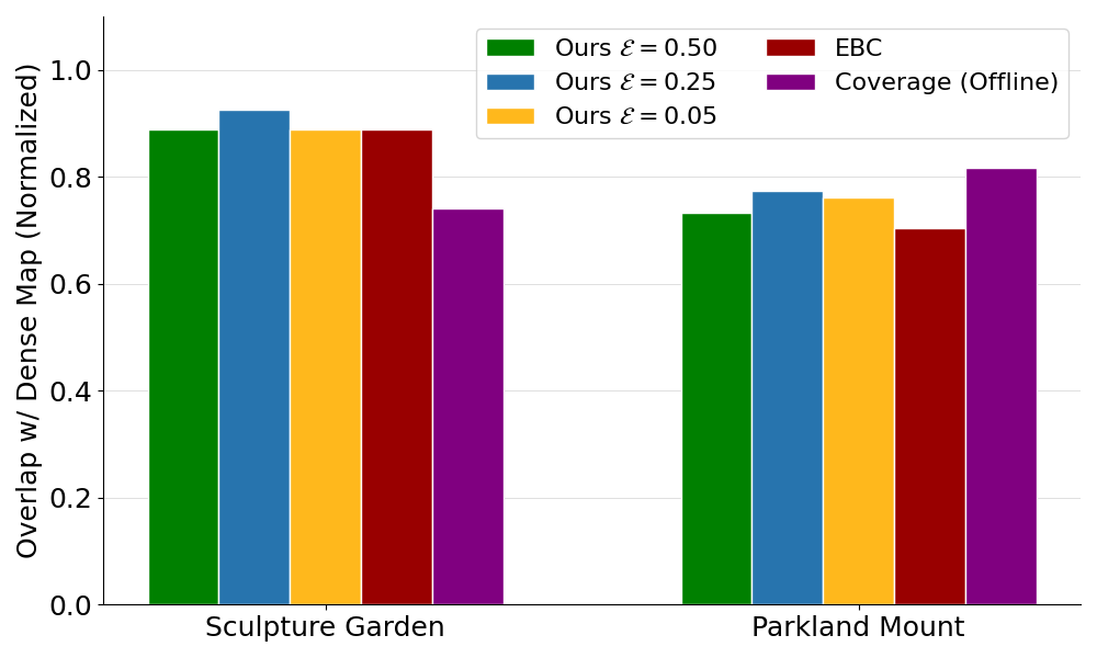
The first experiment seeks to find the best function for quantifying informativeness in geometric map distillation and studies the effects of the reduced set selection threshold parameter . We consider three possible variants: a direct implementation of descriptor coverage Equation 6, Exemplar-Based Clustering (EBC) Equation 8, and Continuous Exemplar-Based Clustering (CEBC, Ours) Equation 10. CEBC was further split into three variants with reduced set thresholds of , , and . Each function was optimized using the greedy algorithm to isolate results from any bias present in streaming submodular optimization. The datasets used were the semi-urban outdoor Sculpture Garden and Parkland Mount from [58]. To measure informativeness, the overlap between each function’s output map and a dense comparison map is used. The number of scans used in output maps was increased until any output exceeded 50% overlap. The overlap percent for each output was then normalized with an optimal result generated by greedily selecting scans that overlap with the dense map.
Results from the first experiment are seen in Fig. 8 where CEBC performs near the optimal across both datasets and with multiple reduced set thresholds, EBC performs well on Sculpture Garden, and coverage performs well on Parkland Mount. Normalized overlap percentages for Sculpture Garden were 89%, 93%, 89%, 89%, and 74% for CEBC with , , , EBC, and coverage respectively. Normalized overlap for Parkland Mount was 73%, 78%, 76%, 70%, and 82% for the five variants respectively. Increasing the reduced set threshold from to reduced overlap, suggesting that higher thresholds discard useful information. However, CEBC with all reduced set thresholds equaled or exceeded EBC, indicating that the continuous trajectory assumption helped quantify informativeness. CEBC also compares favorably with the coverage function which performed well on Parkland Mount but poorly on Sculpture Garden. This inconsistency arose because the coverage function only rewards self-dissimilar solutions, making it less robust. This resulted in lower overlap on the Sculpture Garden dataset which had more sequential descriptors further than 0.25 apart (48 vs. 32, Fig. 4).


scans, Courtyard maps made with twelve scans, and Lab maps made with eight scans.

CEBC also uses a reduced input set to reduce function evaluation time as shown in Fig. 9. For CEBC with , , and EBC the final input set size for the Sculpture Garden was 753, 1256, 3376, and 3575 scans respectively. The final average evaluation time for each variant was 0.0057, 0.0087, 0.0219, and 0.0228 milliseconds showing a strong correlation between input set size and function evaluation time. Compared to EBC, CEBC with the best threshold from Fig. 8, , saw an 84% reduction in average evaluation time and 65% reduction in input set size. Note that the greedy algorithm requires evaluations to find a solution, so a solution with 25 elements would require 2038 ms of optimization for EBC and 273 ms for CEBC with .
VII-B Dynamic Reordering Effectiveness Ablation Study


The second experiment highlights the benefits of dynamic reordering and compares the relative strengths and weaknesses of multiple approximation functions used to generate ordering scores. In addition to the approximations presented in Section V-C (the pairwise information descriptor approximation Equation 16 and heuristic pose approximation Equation 13), we also evaluate a third approximation, which takes the sum of both the pairwise information descriptor and pose approximations. An ablation study compares OptMap using these three approximation functions with the baseline Sieve-Streaming algorithm, random element selection, and the heuristic solution with even spacing described by Algorithm 6. Sieve-Streaming is OptMap with no dynamic reordering but has identical initial solution value bounds. All methods use input sets filtered by Algorithm 2.
Each optimization method generated ten distilled maps on KITTI 05 [7] and two custom datasets collected at UCLA with dense maps shown in Fig. 11. KITTI 05 is a medium length dataset (2736 scans) collected on a fast moving car with no significant bias caused by remapping. Courtyard (Fig. 11 left) introduces a bias to the input set by repeating a small loop fifteen times before making a single mapping pass away from the loop. The bias in the input set is the result of the loop being significantly overrepresented, with the loop accounting for 86% of collected scans but only 31% of the unique distance traveled. Finally, Lab (Fig. 11 right) introduces input set bias by mapping the inside south and north walls of a lab space with four passes each. Scans in the Lab dataset were collected on either side of a thin wall and garage door to stress the position-based CEBC approximation. The UCLA datasets are meant to show the value of dynamic reordering by biasing the input sets. Although this bias is uncommon in open-source datasets, it is not uncommon in practical applications where mapping sessions revisit the same location several times or remain stationary. The output map size for each dataset is hand-picked, with fifty scans used for KITTI 05, twelve scans used for Courtyard, and eight scans used for Lab.
The average overlap percent and its standard deviation for all three datasets are presented in Fig. 10. We normalized the results by the highest performing method for each dataset. All methods are expected to perform well on KITTI 05, but the fast moving car and relatively self-similar street environment stressed the descriptor-based approximation method. The descriptor, pose, and combined dynamic reordering methods have normalized average overlaps of 93.8%, 100%, and 99.0%, with normalized standard deviations of 3.2%, 2.4%, and 1.5% respectively. Sieve-Streaming, random, and the evenly spaced heuristic had normalized average overlaps of 89.3%, 89.1%, and 97.4% and standard deviations of 2.9% and 3.9% (the heuristic is deterministic and hence has no variance). We note that the -suboptimality bound is reached on the UCLA datasets using only 1-3 scans, so Sieve-Streaming performs similarly to random selection in all cases.
Courtyard is meant to demonstrate the strengths of dynamic reordering, which are emphasized by the visual results presented in Fig. 12. The first three panels of Fig. 12 are representative maps from the descriptor, pose, and combined dynamic reordering methods where multiple scans and sufficient coverage of the single pass are present for all three methods. The final three panels show representative maps from Sieve-Streaming, random, and the evenly spaced heuristic; each contain very few scans and minimal coverage from the single pass. The qualitative results match the overlap and standard deviations presented in Fig. 10. The average normalized overlaps are 97.1%, 97.6%, and 100% for the descriptor, pose, and combined approximation dynamic reordering, and the average normalized standard deviations are 2.5%, 2.4%, and 1.6%. In contrast, the average normalized overlaps for Sieve-Streaming, random, and the evenly spaced heuristic are 80.0%, 82.0%, and 87.0%. The average normalized standard deviations for Sieve-Streaming and random are 6.0% and 9.7%. Both Fig. 12 and Fig. 10 show that the value of dynamic reordering increases when an input set contains redundantly mapped areas. In the context of field operations, this is most apparent in providing summary maps when a robot has patrolled the same area many times, but then explores a new environment, i.e., a patrol task followed by a reconnaissance task.

The Lab dataset highlights the strengths of the pairwise information descriptor approximation for dynamic reordering, as it preserves scene context when scans from different environments are collected in close proximity. The average normalized overlap percents for the descriptor, pose, and combined methods are 100%, 88.0%, and 97.7% with standard deviations of 7.4%, 13.9%, and 5.3% respectively. The pose approximation had a significantly worse average and higher standard deviation because scans from either side of a thin wall will be scored similarly despite capturing significantly different environments, as shown in Fig. 13. This indicates that descriptors are best in structured environments where small pose differences can lead to large scene changes, and pose approximation is best in outdoor mapping where descriptors are less capable of learning unstructured environments. Sieve-Streaming and random had low average normalized overlap with 85.3% and 75.0% with particularly high standard deviation with 18.3% and 15.1%. The evenly spaced heuristic had a normalized overlap of 89.9%, which matches the trend of the evenly spaced heuristic outperforming Sieve-Streaming, Random, and either the descriptor or pose approximation in datasets that stress the approximation. Across all three datasets the combined approximation is best or near best, indicating that it preserves the relative strengths of the pose and descriptor approximation without suffering in edge cases where those particular approximations fail.
| Dataset | |||||||
| (Num. Scans) | Distilled Map Size | (1) Opt. [ms] | (1) Load [ms] | (1) Total [ms] | (2) Opt. [ms] | (2) Load [ms] | (2) Total [ms] |
| Oxford Spires Obs. Quarter Seq. 1 [60] (2,894 scans) | 25 | 2.2 | 65.2 | 67.4 | 14.0 | 68.0 | 82.0 |
| 50 | 4.1 | 123.6 | 127.7 | 28.9 | 131.1 | 160.0 | |
| 100 | 8.4 | 243.9 | 252.3 | 57.6 | 252.2 | 309.8 | |
| Oxford Spires Blenheim Palace Seq. 3 [60] (6,970 scans) | 25 | 3.8 | 66.8 | 70.6 | 23.0 | 67.7 | 90.7 |
| 50 | 7.0 | 126.4 | 133.4 | 46.5 | 132.6 | 179.1 | |
| 100 | 15.6 | 252.6 | 268.2 | 93.1 | 256.4 | 349.5 | |
| Semantic KITTI 10 [7] (1,224 scans) | 25 | 2.2 | 65.2 | 67.4 | 14.0 | 68.0 | 82.0 |
| 50 | 4.1 | 123.6 | 127.7 | 28.9 | 131.1 | 160.0 | |
| 100 | 8.4 | 243.9 | 252.3 | 57.6 | 252.2 | 309.8 | |
| Semantic KITTI 02 [7] (4,663 scans) | 100 | 26.9 | 405.7 | 432.6 | 67.1 | 411.5 | 478.6 |
| 250 | 229.8 | 859.4 | 1089.2 | 642.5 | 660.7 | 1303.2 | |
| 500 | 329.6 | 1854.9 | 2184.5 | 2224.0 | 803.1 | 3027.1 | |
| Newer College Long Experiment [58] (26,559 scans) | 100 | 80.5 | 363.6 | 444.1 | 493.8 | 354.4 | 848.2 |
| 250 | 186.5 | 896.5 | 1083.0 | 1248.8 | 917.5 | 2166.3 | |
| 500 | 366.7 | 1919.7 | 2286.4 | 2584.4 | 1956.8 | 4541.2 | |
| Forest Loop (34,158 scans) | 100 | 103.8 | 561.6 | 665.4 | 683.8 | 570.0 | 1253.8 |
| 250 | 275.4 | 1389.9 | 1665.3 | 1694.4 | 1405.4 | 3099.8 | |
| 500 | 531.0 | 2672.3 | 3203.3 | 3353.4 | 2712.4 | 6065.8 |


VII-C Real-Time Map Summarization Evaluation

The third experiment tests OptMap’s return time on large LiDAR datasets with and without a priori bounds. By presenting the time to find and return actionable maps, we also highlight OptMap’s online map distillation capability in the most challenging scenarios with large input set sizes. This experiment distills three small datasets using maps with 25, 50, and 100 scans: Oxford Spires Observatory Quarter Sequences 1 and 3 [60], and Semantic KITTI Sequence 10 [7]. Three larger datasets are distilled using 100, 250, and 500 scans: Semantic KITTI Sequence 02, the Newer College Dataset Long Experiment [58], and Forest Loop, a custom dataset collected in an unstructured forest environment. Load times are directly influenced by the number of points in each scan, which in turn is determined by the number of beams in the sensor. Oxford Spires used a 64-beam Hesai QT64, KITTI used a 64-beam Velodyne HDL-64E, Newer College used a 64-beam Ouster OS1, and Forest Loop used a 128-beam Ouster OS1. The two largest sessions are Newer College Dataset’s Long Experiment [58] and Forest Loop, which contain 26,559 and 34,158 scans representing 44 and 28.5 minutes (or 18.6 and 34 GB) of mapping respectively. OptMap was run five times for each configuration with negligible variation ( ms total max) in either the optimization or map loading time.
The optimization, map loading, and total times for all six datasets are presented in Table I. The third through fifth columns (labeled method 1) used a priori bounds and the sixth through eighth (labeled method 2) did not. The percent of total time saved by the a priori bounds across the three smaller datasets was between 19-24, but the average percent saved across the three larger was 18-49. The dramatic increase in time saved is due to the fact that tighter bounds reduce the number of solution sets that need to be maintained for larger input sets. The total time increases linearly with the distilled map size due to linear increases in both optimization and map loading times. Semantic KITTI is a challenging dataset for OptMap because it is collected on a relatively fast moving car. This stresses the assumption that sequential descriptors are similar and thus results in larger input sets.
Summarization is a key application for OptMap, with visual results presented in Figs. 15, 14 and 16. Figure 15 demonstrates generated summary maps with flexible size, where size-constrained summarization could be valuable for bandwidth-aware multi-robot map sharing or global place recognition. Figure 14 shows a high-fidelity and extremely detailed map of the Newer College Dataset Long Experiment generated by OptMap. The inset shows a detailed map that is not usually available from LiDAR SLAM due to the computation and memory load required for maintaining dense maps. Finally, Fig. 16 shows the largest OptMap distilled map by number of input scans. We separate optimization and map loading times in Table I to highlight the fact that a significant portion of OptMap’s total time comes from needing to load LiDAR scans. This demonstrates the need for indirect optimization (i.e., no point-to-point computations) in geometric map distillation, which is further highlighted in the following result.
VII-D Application: Geometric Change Detection
The final result highlights a practical application of OptMap for online change detection. We assume a human operator has identified a particular location that has been mapped multiple times to check for objects that have appeared, disappeared, or moved. Changes can be identified by comparing two point clouds from different times, where the distance from each point in the before (resp. after) map to its nearest neighbor in the after (resp. before) map is used to determine if the point is a change. Results are better when the two maps are dense (i.e., the average distance between points is small) and thus change detection is usually handled by offline algorithms such as [40]. However, for patrol or search-and-rescue missions, online change detection may be very pertinent for mission planning (e.g., a set of fresh footprints are detected). Although some geometric change detection algorithms are real-time [56, 62, 44, 43], they only compare a single sensor output to a map and therefore lack the density to detect subtle details. A full comparison is beyond the scope of this work, but to the best of our knowledge, there is no current online geometric change detection algorithm which utilizes dense before and after maps.
A dense before submap generated by OptMap from a junction in a dataset collected at the Army Research Laboratory is shown in Fig. 17 with the before, after, and difference map shown in Fig. 1(b). The operator defined the position and time bounds for the before and after map given knowledge of the mapping session. Points in either map are labeled as a potential change if the nearest point in the other map is at least 10 cm away. Potential changes are then pruned by a simple noise filter that discards points where the average distance to the nearest 50 potential change points is more than 5 cm away. This noise filter is meant to discard spurious incorrect changes that might result from mismatched scan lines or field of view differences. The results of change detection are shown on the right of Fig. 17, where two 60 cm tall cases were identified as negative changes, and a 20 cm tall backpack was identified as a positive change with no incorrect detections. The time to generate each OptMap output with 60 scans was just 196 ms.
This result is remarkable because the change detection maps cannot be generated using a simple downsampling method (i.e., voxelization). The left image in Fig. 17 shows the OptMap before map and center shows a voxelized dense map (with resolution 0.25 m). This resolution is selected such that the full map for a mapping session up to approximately 5 km could be stored in the available 16 GB of computer memory. The before and after submaps each contain approximately fifteen million points in twenty meters traveled. With approximately 40 bytes per point, the memory burden of saving a global map with equal density would be approximately 15 MB per meter traveled. Such a rate is not feasible as even short sessions that traverse 1 km would demand nearly 15 GB of memory. Current research indicates a push for lightweight, memory optimized SLAM algorithms that save fewer points [61, 24], so OptMap is positioned to supplement these algorithms by providing flexible, online, and application-specific maps such as those shown in Fig. 17.
VIII Conclusion
This work presented OptMap, an online geometric map distillation algorithm that can generate provably near-optimal representative distillation maps from large LiDAR mapping datasets. We propose multiple theoretical and algorithmic innovations which provide a means for quantifying informativeness in geometric maps, and allows for the efficient optimization of such maps. The novel submodular reward function Continuous Exemplar-Based Clustering (CEBC) effectively rewards informativeness with the added ability to significantly reduce the size of input sets and improve computation time via the elimination of sequentially redundant elements. Dynamic reordering is a novel addition to streaming submodular maximization algorithms which uses multiple approximation functions for CEBC to address input order bias. Tight a priori solution bounds further reduce computation time, and basic position and time constraints are introduced to make OptMap immediately useful to several applications including online change detection and multi-robot map sharing. The results demonstrate the efficacy of CEBC, dynamic reordering, and tight a priori bounds across a range of custom and open-source LiDAR datasets. We demonstrate a practical application for OptMap in online change detection and envision several other similar novel capabilities that could be derived from OptMap.
Future work on OptMap can incorporate higher quality learned descriptors and other similarity metrics for improved distillation results across a wider variety of environments. Although the descriptors in this work were shown to accurately describe a LiDAR scan, descriptors that better discriminate based on local features (i.e., groups of points from the same object) could enable more sophisticated submodular functions for selecting localization submaps or sharing relevant scans without knowing relative poses. Additional work in generalizing dynamic reordering could yield a novel generalized streaming submodular maximization algorithm that uses limited a priori information to address significant forms of input order bias in computationally efficient methods. Improved functionality could also be derived from general matroid constraints. For example, a knapsack constraint could enable input sets with multiple contributing sensor types, and set coverage constraints could allow for minimum size solutions which satisfy a defined coverage criterion. Such innovations can lead to a tighter, bidirectional integration between geometric mapping and the downstream autonomy algorithms or operators that rely on compact and informative geometric maps.
Appendix
Proof of Corollary 1.
For each outlier and its corresponding source set , , the difference in the distance to an arbitrary solution is because the maximum distance between points on a hypersphere is . Without loss of generality, assume that the outliers are the final elements of the reduced set, where elements of the full input set may still exist between these outliers. Restating the third line of Theorem 1 then separating the sum over the reduced set into inliers and outliers is then
where we can apply Lemma 1 to the first elements and to the final outliers. This results in
Using and , we get
as desired. ∎
References
- [1] (2022) An optimal streaming algorithm for submodular maximization with a cardinality constraint. Mathematics of Operations Research 47 (4), pp. 2667–2690. Cited by: §II-B.
- [2] (2023) Padloc: lidar-based deep loop closure detection and registration using panoptic attention. IEEE Robotics and Automation Letters 8 (3), pp. 1319–1326. Cited by: §I, §II-A.
- [3] (2014) Streaming submodular maximization: massive data summarization on the fly. In Proceedings of the 20th ACM SIGKDD International Conference on Knowledge Discovery and Data Mining, pp. 671–680. Cited by: §I, §II-B, §III-A, §III-A, §V-A, Proposition 1, Algorithm 1.
- [4] (2024) Multi-robot active graph exploration with reduced pose-slam uncertainty via submodular optimization. In 2024 IEEE/RSJ International Conference on Intelligent Robots and Systems (IROS), pp. 10229–10236. Cited by: §II-B.
- [5] (2023) Dynamic constrained submodular optimization with polylogarithmic update time. In International Conference on Machine Learning, pp. 1660–1691. Cited by: §II-B.
- [6] (2024) Dynamic algorithms for matroid submodular maximization. In Proceedings of the 2024 Annual ACM-SIAM Symposium on Discrete Algorithms (SODA), pp. 3485–3533. Cited by: §II-B.
- [7] (2019) SemanticKITTI: A Dataset for Semantic Scene Understanding of LiDAR Sequences. In Proc. of the IEEE/CVF International Conf. on Computer Vision (ICCV), Cited by: Figure 10, Figure 10, §VII-B, §VII-C, TABLE I, TABLE I, §VII.
- [8] (2017) Deep learning. Vol. 1, MIT press Cambridge, MA, USA. Cited by: §IV-C.
- [9] (2023) Occupancy grid mapping without ray-casting for high-resolution lidar sensors. IEEE Transactions on Robotics. Cited by: §II-A.
- [10] (2021) Ikd-tree: an incremental kd tree for robotic applications. arXiv preprint arXiv:2102.10808. Cited by: §II-A.
- [11] (2018) Attention and anticipation in fast visual-inertial navigation. IEEE Transactions on Robotics 35 (1), pp. 1–20. Cited by: §II-B.
- [12] L. Carlone, A. Kim, T. Barfoot, D. Cremers, and F. Dellaert (Eds.) (2025) SLAM Handbook. from localization and mapping to spatial intelligence. Cambridge University Press. Cited by: §II-A.
- [13] (2015) Submodular maximization meets streaming: matchings, matroids, and more. Mathematical Programming 154, pp. 225–247. Cited by: §II-B.
- [14] (2015) Streaming algorithms for submodular function maximization. In Automata, Languages, and Programming: 42nd International Colloquium, ICALP 2015, Kyoto, Japan, July 6-10, 2015, Proceedings, Part I 42, pp. 318–330. Cited by: §I, §II-B.
- [15] (2023) Direct lidar-inertial odometry: lightweight lio with continuous-time motion correction. In 2023 IEEE International Conference on Robotics and Automation (ICRA), pp. 3983–3989. Cited by: §I, §II-A, §VII, footnote 4.
- [16] (2022) On the complexity of dynamic submodular maximization. In Proceedings of the 54th Annual ACM SIGACT Symposium on Theory of Computing, pp. 1685–1698. Cited by: §II-B.
- [17] (2022) OverlapNet: a siamese network for computing lidar scan similarity with applications to loop closing and localization. Autonomous Robots, pp. 1–21. Cited by: §I, §II-A, §IV-A.
- [18] (2021) Anchor selection for slam based on graph topology and submodular optimization. IEEE Transactions on Robotics 38 (1), pp. 329–350. Cited by: §II-B.
- [19] (2018) Delight: an efficient descriptor for global localisation using lidar intensities. In 2018 IEEE International Conference on Robotics and Automation (ICRA), pp. 3653–3660. Cited by: §II-A.
- [20] (2019) Distributed matroid-constrained submodular maximization for multi-robot exploration: theory and practice. Autonomous Robots 43, pp. 485–501. Cited by: §II-B.
- [21] (2019) Communication-efficient planning and mapping for multi-robot exploration in large environments. IEEE Robotics and Automation Letters 4 (2), pp. 1715–1721. Cited by: §II-B.
- [22] (2011) Submodular meets spectral: greedy algorithms for subset selection, sparse approximation and dictionary selection. In Proceedings of the 28th International Conference on International Conference on Machine Learning, pp. 1057–1064. Cited by: §II-B.
- [23] (2013) Summarization through submodularity and dispersion. In Proceedings of the 51st Annual Meeting of the Association for Computational Linguistics (Volume 1: Long Papers), pp. 1014–1022. Cited by: §II-B.
- [24] (2025) LiDAR inertial odometry and mapping using learned registration-relevant features. In 2025 IEEE International Conference on Robotics and Automation (ICRA), pp. 359–366. Cited by: §II-A, §VII-D.
- [25] (2022) Submodular maximization with limited function access. IEEE Transactions on Automatic Control 68 (9), pp. 5522–5535. Cited by: §III, Definition 3.
- [26] (2007) Non-metric affinity propagation for unsupervised image categorization. In 2007 IEEE 11th International Conference on Computer Vision, pp. 1–8. Cited by: §II-B.
- [27] (2020) Fairness in streaming submodular maximization: algorithms and hardness. Advances in Neural Information Processing Systems 33, pp. 13609–13622. Cited by: §II-B.
- [28] (2011) Beyond keyword search: discovering relevant scientific literature. In Proceedings of the 17th ACM SIGKDD international conference on Knowledge discovery and data mining, pp. 439–447. Cited by: §II-B.
- [29] (2011) Maximizing non-monotone submodular functions. SIAM Journal on Computing 40 (4), pp. 1133–1153. Cited by: §II-B.
- [30] (2018) Do less, get more: streaming submodular maximization with subsampling. Advances in Neural Information Processing Systems 31. Cited by: §I, §II-B.
- [31] (2005) Submodular functions and optimization. Elsevier. Cited by: §I, §II-B.
- [32] (2020) Semantics for robotic mapping, perception and interaction: a survey. Foundations and Trends® in Robotics 8 (1–2), pp. 1–224. Cited by: §II-A.
- [33] (2017) Distributed submodular maximization with limited information. IEEE Transactions on Control of Network Systems 5 (4), pp. 1635–1645. Cited by: §II-B.
- [34] (2010) Constrained non-monotone submodular maximization: offline and secretary algorithms. In International Workshop on Internet and Network Economics, pp. 246–257. Cited by: §II-B.
- [35] (1989) Multilayer feedforward networks are universal approximators. Neural networks 2 (5), pp. 359–366. Cited by: §IV-C.
- [36] (2013) OctoMap: an efficient probabilistic 3D mapping framework based on octrees. Autonomous Robots. External Links: Link, Document Cited by: §II-A.
- [37] (2009) Finding groups in data: an introduction to cluster analysis. John Wiley & Sons. Cited by: §IV-B, §IV-B.
- [38] (2019) Submodular streaming in all its glory: tight approximation, minimum memory and low adaptive complexity. In International Conference on Machine Learning, pp. 3311–3320. Cited by: §I, §II-B.
- [39] (2019) Reliable graphs for slam. The International Journal of Robotics Research 38 (2-3), pp. 260–298. Cited by: §II-B.
- [40] (2022) Lt-mapper: a modular framework for lidar-based lifelong mapping. In 2022 International Conference on Robotics and Automation (ICRA), pp. 7995–8002. Cited by: §VII-D.
- [41] (2021) PLGRIM: hierarchical value learning for large-scale exploration in unknown environments. In Proceedings of the International Conference on Automated Planning and Scheduling, Vol. 31, pp. 652–662. Cited by: §II-A.
- [42] (2021) Minkloc3d: point cloud based large-scale place recognition. In Proceedings of the IEEE/CVF Winter Conference on Applications of Computer Vision, pp. 1790–1799. Cited by: §I, §II-A.
- [43] (2024) Change of scenery: unsupervised lidar change detection for mobile robots. In 2024 21st Conference on Robots and Vision (CRV), External Links: Document Cited by: §VII-D.
- [44] (2024) LaserSAM: zero-shot change detection using visual segmentation of spinning lidar. arXiv preprint arXiv:2402.10321. Cited by: §VII-D.
- [45] (2011) Efficient information-theoretic graph pruning for graph-based slam with laser range finders. In 2011 IEEE/RSJ International Conference on Intelligent Robots and Systems, pp. 865–871. Cited by: §II-B.
- [46] (2010) Concise formulas for the area and volume of a hyperspherical cap. Asian Journal of Mathematics & Statistics 4 (1), pp. 66–70. Cited by: §IV-B, §V-C.
- [47] (2024) Computation-aware multi-object search in 3d space using submodular tree. In 2024 IEEE International Conference on Robotics and Automation (ICRA), pp. 5956–5962. Cited by: §II-B.
- [48] (2011) A class of submodular functions for document summarization. In Proceedings of the 49th annual meeting of the association for computational linguistics: human language technologies, pp. 510–520. Cited by: §II-B, §IV-B, §IV.
- [49] (2022) Overlaptransformer: an efficient and yaw-angle-invariant transformer network for lidar-based place recognition. IEEE Robotics and Automation Letters 7 (3), pp. 6958–6965. Cited by: §I, §II-A.
- [50] (2005) Accelerated greedy algorithms for maximizing submodular set functions. In Optimization Techniques: Proceedings of the 8th IFIP Conference on Optimization Techniques Würzburg, September 5–9, 1977, pp. 234–243. Cited by: §II-B.
- [51] (2015) Lazier than lazy greedy. In Proceedings of the AAAI Conference on Artificial Intelligence, Vol. 29. Cited by: §II-B.
- [52] (2016) Fast constrained submodular maximization: personalized data summarization. In International Conference on Machine Learning, pp. 1358–1367. Cited by: §II-B.
- [53] (2020) Dynamic submodular maximization. Advances in Neural Information Processing Systems 33, pp. 9806–9817. Cited by: §II-B.
- [54] (1978) An analysis of approximations for maximizing submodular set functions—i. Mathematical programming 14, pp. 265–294. Cited by: §I, §II-B, §III.
- [55] (1978) Best algorithms for approximating the maximum of a submodular set function. Mathematics of operations research 3 (3), pp. 177–188. Cited by: §I, §II-B, §III.
- [56] (2022) POCD: probabilistic object-level change detection and volumetric mapping in semi-static scenes. In Robotics: Science and Systems (RSS), Cited by: §VII-D.
- [57] (2024) Approximate environment decompositions for robot coverage planning using submodular set cover. In 2024 IEEE 63rd Conference on Decision and Control (CDC), pp. 7528–7533. Cited by: §II-B, §IV-B.
- [58] (2020) The newer college dataset: handheld lidar, inertial and vision with ground truth. In 2020 IEEE/RSJ International Conference on Intelligent Robots and Systems (IROS), Vol. , pp. 4353–4360. External Links: Document Cited by: Figure 4, Figure 4, Figure 8, Figure 8, §VII-A, §VII-C, TABLE I, §VII.
- [59] (2020) Lio-sam: tightly-coupled lidar inertial odometry via smoothing and mapping. In 2020 IEEE/RSJ International Conference on Intelligent Robots and Systems (IROS), pp. 5135–5142. Cited by: §II-A.
- [60] (2025) The oxford spires dataset: benchmarking large-scale lidar-visual localisation, reconstruction and radiance field methods. International Journal of Robotics Research. Cited by: §VII-C, TABLE I, TABLE I, §VII.
- [61] (2025) Submodular optimization for keyframe selection & usage in slam. In 2025 IEEE International Conference on Robotics and Automation (ICRA), pp. 5033–5039. Cited by: §I, §II-A, §II-B, §VII-D.
- [62] (2017) Reliable real-time change detection and mapping for 3D lidars. In 2017 IEEE International Symposium on Safety, Security and Rescue Robotics (SSRR), pp. 81–87. External Links: Document Cited by: §VII-D.
- [63] (2022) Fast-lio2: fast direct lidar-inertial odometry. IEEE Transactions on Robotics 38 (4), pp. 2053–2073. Cited by: §II-A.
- [64] (2018) Hierarchical probabilistic fusion framework for matching and merging of 3-d occupancy maps. IEEE Sensors Journal 18 (21), pp. 8933–8949. Cited by: §II-A.
- [65] (2019) A multilevel fusion system for multirobot 3-d mapping using heterogeneous sensors. IEEE Systems Journal 14 (1), pp. 1341–1352. Cited by: §II-A.
- [66] (2016) Submodular optimization with routing constraints. In Proceedings of the AAAI conference on artificial intelligence, Vol. 30. Cited by: §II-B.
- [67] (2014) LOAM: lidar odometry and mapping in real-time.. In Robotics: Science and Systems, Vol. 2, pp. 1–9. Cited by: §II-A.