跳到论文正文
W Papers独立论文阅读器 arXiv:2512.07443 论文正文 计算阅读时间 · 0%
引用这篇论文根据当前论文元数据生成,正式投稿前建议核对。


A multivariate extension of Azadkia-Chatterjee’s rank coefficient

Wenjie Huang1, Zonghan Li1 and Yuhao Wang1,2

1 Institute for Interdisciplinary Information Sciences, Tsinghua University, Beijing, China
2 Shanghai Qi Zhi Institute, Shanghai, China
The authors are listed in alphabetical order, correspondence should be addressed to Yuhao Wang: yuhaow@tsinghua.edu.cn
Abstract

The Azadkia-Chatterjee coefficient is a rank-based measure of dependence between a random variable Y∈ℝY\in\mathbb{R} and a random vector 𝒁∈ℝdZ\boldsymbol{Z}\in\mathbb{R}^{d_{Z}}. This paper proposes a multivariate extension that measures the dependence between random vectors 𝒀∈ℝdY\boldsymbol{Y}\in\mathbb{R}^{d_{Y}} and 𝒁∈ℝdZ\boldsymbol{Z}\in\mathbb{R}^{d_{Z}}, based on nn i.i.d. samples. The proposed coefficient converges almost surely to a limit with the following properties: i) it lies in [0,1][0,1]; ii) it is equal to zero if and only if 𝒀\boldsymbol{Y} and 𝒁\boldsymbol{Z} are independent; and iii) it is equal to one if and only if 𝒀\boldsymbol{Y} is almost surely a function of 𝒁\boldsymbol{Z}. Remarkably, the only assumption required by this convergence is that 𝒀\boldsymbol{Y} is not almost surely a constant vector. We further prove that under the same mild condition and after a proper scaling, this coefficient converges in distribution to a standard normal random variable when 𝒀\boldsymbol{Y} and 𝒁\boldsymbol{Z} are independent. This asymptotic normality result allows us to construct a Wald-type hypothesis test of independence based on this coefficient. To compute this coefficient, we propose a merge sort based algorithm that runs in O​(n​(log⁡n)dY)O(n(\log n)^{d_{Y}}). Finally, we show that it can be used to measure the conditional dependence between 𝒀\boldsymbol{Y} and 𝒁\boldsymbol{Z} conditional on a third random vector 𝑿\boldsymbol{X}, and prove that the measure is monotonic with respect to the deviation from an independence distribution under certain model restrictions.

1 Introduction

Measuring the dependence (and conditional dependence) of random variables is a fundamental task in statistics. Classical coefficients include Pearson’s correlation coefficient, Spearman’s ρ\rho, and Kendall’s τ\tau. Recently, there has been growing interest in developing new dependence measures tailored to specific applications; see Chatterjee (2021); Josse and Holmes (2016) for surveys. However, as argued by Chatterjee (2021), most existing measures suffer from two drawbacks: they are built to test independence rather than quantify the strength of dependence, and they lack simple asymptotic null distributions, so computationally intensive procedures such as permutation or bootstrap tests are required to obtain p-values.

In light of these issues, Chatterjee (2021) recommended to propose a coefficient that is

“(a) as simple as the classical coefficients like Pearson’s correlation or Spearman’s correlation, and yet (b) consistently estimates some simple and interpretable measure of the degree of dependence between the variables, which is 0 if and only if the variables are independent and 1 if and only if one is a measurable function of the other, and (c) has a simple asymptotic theory under the hypothesis of independence, like the classical coefficients”

These criteria, especially (b), seem very natural. In fact, requirement similar to (b) was already discussed by Rényi (1959):

“It is natural to choose the range [0,1][0,1] and to make correspond the value 11 to strict dependence and thus 0 to independence.”

In the same paper, Chatterjee (2021) further showed that at least in the univariate case, a coefficient satisfying these criteria is possible. More specifically, they introduced a coefficient that converges almost surely to a measure of dependence between two random variables Y,Z∈ℝY,Z\in\mathbb{R} – a measure previously examined by Dette et al. (2013); Gamboa et al. (2018). Remarkably, this measure satisfies (b), and the convergence of the coefficient in Chatterjee (2021) requires only that YY is not almost surely a constant. Moreover, under the null hypothesis where Y⟂⟂ZY\mathchoice{\mathrel{\hbox to0.0pt{$\displaystyle\perp$\hss}\mkern 2.0mu{\displaystyle\perp}}}{\mathrel{\hbox to0.0pt{$\textstyle\perp$\hss}\mkern 2.0mu{\textstyle\perp}}}{\mathrel{\hbox to0.0pt{$\scriptstyle\perp$\hss}\mkern 2.0mu{\scriptstyle\perp}}}{\mathrel{\hbox to0.0pt{$\scriptscriptstyle\perp$\hss}\mkern 2.0mu{\scriptscriptstyle\perp}}}Z, they proved that this coefficient is asymptotically normal under the same mild condition. The proposed coefficient is a rank-based approach constructed using only the ranks of the i.i.d. samples of two random variables YY and ZZ. This rank-based nature also confers two key advantages: robustness to outliers and contamination; and invariant under certain data transformations, such as linear transformations (see e.g. Section 2).

As an extension, Azadkia and Chatterjee (2021) relaxed the dimensionality restriction of ZZ, allowing it to be a random vector 𝒁∈ℝdZ\boldsymbol{Z}\in\mathbb{R}^{d_{Z}}. Moreover, they showed that the asymptotic limit of the proposed coefficient, denoted as TAC​(Y,𝒁)T^{\textrm{AC}}(Y,\boldsymbol{Z}), has the property that, given a third vector 𝑿∈ℝdX\boldsymbol{X}\in\mathbb{R}^{d_{X}}, TAC​(Y,(𝒁,𝑿))T^{\textrm{AC}}(Y,(\boldsymbol{Z},\boldsymbol{X})) and TAC​(Y,𝑿)T^{\textrm{AC}}(Y,\boldsymbol{X}) satisfy

TAC​(Y,(𝒁,𝑿))≥TAC​(Y,𝑿)&TAC​(Y,(𝒁,𝑿))=TAC​(Y,𝑿)​if.f.​Y⟂⟂𝒁∣𝑿.T^{\textrm{AC}}(Y,(\boldsymbol{Z},\boldsymbol{X}))\geq T^{\textrm{AC}}(Y,\boldsymbol{X})\;\&\;T^{\textrm{AC}}(Y,(\boldsymbol{Z},\boldsymbol{X}))=T^{\textrm{AC}}(Y,\boldsymbol{X})\;\textrm{if.f.}\;Y\mathchoice{\mathrel{\hbox to0.0pt{$\displaystyle\perp$\hss}\mkern 2.0mu{\displaystyle\perp}}}{\mathrel{\hbox to0.0pt{$\textstyle\perp$\hss}\mkern 2.0mu{\textstyle\perp}}}{\mathrel{\hbox to0.0pt{$\scriptstyle\perp$\hss}\mkern 2.0mu{\scriptstyle\perp}}}{\mathrel{\hbox to0.0pt{$\scriptscriptstyle\perp$\hss}\mkern 2.0mu{\scriptscriptstyle\perp}}}\boldsymbol{Z}\mid\boldsymbol{X}. (1)

This allows us to use TACT^{\textrm{AC}} to measure not only dependence, but also conditional dependence of YY and 𝒁\boldsymbol{Z} given a third vector 𝑿∈ℝdX\boldsymbol{X}\in\mathbb{R}^{d_{X}}. This new coefficient is now widely called the “Azadkia–Chatterjee rank coefficient” (AC coefficient). In a follow up study, Shi et al. (2024) proved the asymptotic normality of the new coefficient when YY and 𝒁\boldsymbol{Z} are independent, under the additional assumption that YY is continuous and 𝒁\boldsymbol{Z} is absolutely continuous. In another follow up work (Lin and Han, 2022), the authors further analyzed the asymptotic normality of the AC coefficient when YY and 𝒁\boldsymbol{Z} are not independent. Ansari and Fuchs (2022) further extended AC coefficient to the case where 𝒀∈ℝdY\boldsymbol{Y}\in\mathbb{R}^{d_{Y}}, subject to that each component of 𝒀\boldsymbol{Y} is not almost surely a constant, as well as some additional regularity conditions of 𝒀\boldsymbol{Y}. While it represents an important extension, it remains unclear whether the estimation bias of their proposed coefficient is of order o​(1/n)o(1/\sqrt{n}) under the null hypothesis of independence. Consequently, their coefficient cannot be used directly to construct a valid Wald-type hypothesis test for independence, unlike classical correlation coefficients.

Alongside extensions of AC coefficients, another line of research has pursued an alternative strategy for developing rank-based multivariate dependence coefficients: leveraging optimal transport techniques. This strategy has been the subject of intensive research over the past decade. The common approach in this line of work first employs optimal transport-based techniques to construct a so-called “multivariate rank” (or “Monge-Kantorovich rank”) (Chernozhukov et al., 2017; Hallin et al., 2021), and then uses this rank to replace the traditional rank for coefficient construction. Famous applications of this idea include Deb and Sen (2023); Deb et al. (2020, 2024); Shi et al. (2022); Mordant and Segers (2022); see e.g. Han (2021); Chatterjee (2024) for recent surveys. Under the null hypothesis that 𝒀\boldsymbol{Y} and 𝒁\boldsymbol{Z} are independent, these rank-based coefficients are usually guaranteed to converge to an asymptotic distribution (not necessarily normal), so that one can construct asymptotically valid tests for testing independence based on these coefficients.

While this progress is encouraging, the asymptotic null distribution of these rank-based approaches are all derived under the extra assumption that both 𝒀\boldsymbol{Y} and 𝒁\boldsymbol{Z} are absolutely continuous with respect to the Lebesgue measure. Moreover, when 𝒀\boldsymbol{Y} and 𝒁\boldsymbol{Z} are dependent, these coefficients either require extra assumptions on the joint distribution of 𝒀\boldsymbol{Y} and 𝒁\boldsymbol{Z} in order to ensure its asymptotic convergence, or cannot satisfy all the desired properties in criterion (b). Finally, to the best of our knowledge, none of these coefficients satisfy (1), and thus cannot be easily extended to measure conditional dependence.

In light of these works, a natural question is: can we construct a rank-based multivariate dependence coefficient that satisfies all the criteria (a)–(c) advocated by Chatterjee (2021), as well as (1), without invoking any distributional assumption? In this paper, we propose a new multivariate extension of Azadkia-Chatterjee’s rank coefficient to overcome these barriers. We prove that it converges almost surely to a measure of dependence between 𝒀\boldsymbol{Y} and 𝒁\boldsymbol{Z} as long as 𝒀\boldsymbol{Y} is not almost surely a constant vector. Moreover, this measure inherits the criterion (b) advocated by Chatterjee (2021), as well as (1), so that it can be used to measure the conditional dependence of 𝒀\boldsymbol{Y} and 𝒁\boldsymbol{Z}, given a third random vector 𝑿\boldsymbol{X}. We also derive the asymptotic null distribution of this coefficient under the hypothesis of independence. Remarkably, our asymptotic null analysis requires only that 𝒀\boldsymbol{Y} is not almost surely a constant, allowing us to yield a valid test based on this coefficient even when 𝒀\boldsymbol{Y} and 𝒁\boldsymbol{Z} are not absolutely continuous. This sheds light on the asymptotic analysis of Shi et al. (2024) even in the univariate YY case. Finally, we further provide a merge sort based algorithm (Knuth, 1997) which can compute this coefficient in time complexity O​(n​(log⁡n)dY)O(n(\log n)^{d_{Y}}), and analyze the monotonicity properties of this dependence measure.

The rest of this article is organized as follows. In Section 2, we review previous results of Azadkia-Chatterjee coefficient in the univariate YY case. In Section 3, we provide a multivariate extension, and analyze its almost sure convergence property. In Section 4, we discuss its asymptotically normality under independence. In Section 5, we discuss how to compute this coefficient, and discuss the properties of this new coefficient. In Sections 6 and 7, we prove the key theoretical findings.

Notations. Given two vectors 𝒂,𝒃∈ℝd\boldsymbol{a},\boldsymbol{b}\in\mathbb{R}^{d}, we write 𝒂∧𝒃\boldsymbol{a}\wedge\boldsymbol{b} as their entrywise minimum (𝒂1∧𝒃1,…,𝒂d∧𝒃d)(\boldsymbol{a}_{1}\wedge\boldsymbol{b}_{1},\ldots,\boldsymbol{a}_{d}\wedge\boldsymbol{b}_{d}), and say that 𝒂≤𝒃\boldsymbol{a}\leq\boldsymbol{b} if 𝒂i≤𝒃i\boldsymbol{a}_{i}\leq\boldsymbol{b}_{i} holds for all i∈[d]i\in[d]. Write ∥⋅∥\|\cdot\| as the ℓ2\ell_{2}-norm. Given a sequence of random variables AnA_{n} and a random variable AA, we write An​→a.s.​AA_{n}\overset{\textrm{a.s.}}{\to}A if AnA_{n} converges to AA almost surely, and An​→𝑑​AA_{n}\overset{d}{\to}A if it converges in distribution.

2 Azadkia-Chatterjee coefficient: preliminaries and property discussions

Consider a random variable Y∈ℝY\in\mathbb{R} and a random vector 𝒁∈ℝdZ\boldsymbol{Z}\in\mathbb{R}^{d_{Z}}, both defined on the same probability space, Azadkia and Chatterjee (2021) proposed to measure the dependence between YY and 𝒁\boldsymbol{Z} via:

TAC​(Y,𝒁):=∫var​(ℙ​(Y≥y∣𝒁))​𝑑μY​(y)∫var​(𝟙​{Y≥y})​𝑑μY​(y),T^{\textrm{AC}}(Y,\boldsymbol{Z}):=\frac{\int\mathrm{var}(\mathbb{P}(Y\geq y\mid\boldsymbol{Z}))d\mu_{Y}(y)}{\int\mathrm{var}(\mathbbm{1}\{Y\geq y\})d\mu_{Y}(y)}, (2)

where μY\mu_{Y} denotes the measure of the marginal distribution of YY. In the rest of this paper, we will also simplify it as TACT^{\textrm{AC}} when the context is clear. Azadkia and Chatterjee (2021) claimed that, as long as YY is not almost surely a constant, TACT^{\textrm{AC}} satisfies the following two properties:

  1. (P1)

    0≤TAC​(Y,𝒁)≤10\leq T^{\textrm{AC}}(Y,\boldsymbol{Z})\leq 1; moreover, TAC​(Y,𝒁)T^{\textrm{AC}}(Y,\boldsymbol{Z}) is equal to 0 if and only if Y⟂⟂𝒁Y\mathchoice{\mathrel{\hbox to0.0pt{$\displaystyle\perp$\hss}\mkern 2.0mu{\displaystyle\perp}}}{\mathrel{\hbox to0.0pt{$\textstyle\perp$\hss}\mkern 2.0mu{\textstyle\perp}}}{\mathrel{\hbox to0.0pt{$\scriptstyle\perp$\hss}\mkern 2.0mu{\scriptstyle\perp}}}{\mathrel{\hbox to0.0pt{$\scriptscriptstyle\perp$\hss}\mkern 2.0mu{\scriptscriptstyle\perp}}}\boldsymbol{Z}; and is equal to 11 if and only if YY is almost surely a function of 𝒁\boldsymbol{Z};

  2. (P2)

    Consider in addition a random vector 𝑿∈ℝdX\boldsymbol{X}\in\mathbb{R}^{d_{X}} on the same probability space as (Y,𝒁)(Y,\boldsymbol{Z}), then TAC​(Y,(𝑿,𝒁))≥TAC​(Y,𝑿)T^{\textrm{AC}}(Y,(\boldsymbol{X},\boldsymbol{Z}))\geq T^{\textrm{AC}}(Y,\boldsymbol{X}), where the equality holds if and only if Y⟂⟂𝒁∣𝑿Y\mathchoice{\mathrel{\hbox to0.0pt{$\displaystyle\perp$\hss}\mkern 2.0mu{\displaystyle\perp}}}{\mathrel{\hbox to0.0pt{$\textstyle\perp$\hss}\mkern 2.0mu{\textstyle\perp}}}{\mathrel{\hbox to0.0pt{$\scriptstyle\perp$\hss}\mkern 2.0mu{\scriptstyle\perp}}}{\mathrel{\hbox to0.0pt{$\scriptscriptstyle\perp$\hss}\mkern 2.0mu{\scriptscriptstyle\perp}}}\boldsymbol{Z}\mid\boldsymbol{X}.

LABEL:p1 matches the criterion (b) mentioned in Chatterjee (2021); LABEL:p2 allows practitioners to use TACT^{\textrm{AC}} to construct a measure of conditional dependence of YY and 𝒁\boldsymbol{Z}, given a third random vector 𝑿\boldsymbol{X}. Moreover, since TACT^{\textrm{AC}} is constructed via the conditional CDF of YY, such structure further reveals the following property:

  1. (P3)

    For any strictly increasing function f​(⋅)f(\cdot) and any invertible h​(⋅)h(\cdot), TAC​(Y,𝒁)=TAC​(f​(Y),h​(𝒁))T^{\textrm{AC}}(Y,\boldsymbol{Z})=T^{\textrm{AC}}(f(Y),h(\boldsymbol{Z})).

LABEL:p3 implies, for example, that TAC​(Y,𝒁)=TAC​(α​Y+β,𝒁)T^{\textrm{AC}}(Y,\boldsymbol{Z})=T^{\textrm{AC}}(\alpha Y+\beta,\boldsymbol{Z}) for any α>0,β∈ℝ\alpha>0,\beta\in\mathbb{R}. Another classical example for strictly monotone function is the logarithmic transformation widely used in genetics studies. In light of LABEL:p2, Azadkia and Chatterjee (2021) proposed to measure the conditional dependence between YY and 𝒁\boldsymbol{Z}, conditional on 𝑿\boldsymbol{X}, via:

TAC, cond​(Y,𝒁∣𝑿):=TAC​(Y,(𝒁,𝑿))−TAC​(Y,𝑿)1−TAC​(Y,𝑿)≡∫𝔼​(var​(ℙ​(Y≥y∣𝒁,𝑿)∣𝑿))​𝑑μY​(y)∫𝔼​(var​(𝟙​{𝒀≥𝒚}∣𝑿))​𝑑μY​(y).T^{\textrm{AC, cond}}(Y,\boldsymbol{Z}\mid\boldsymbol{X}):=\frac{T^{\textrm{AC}}(Y,(\boldsymbol{Z},\boldsymbol{X}))-T^{\textrm{AC}}(Y,\boldsymbol{X})}{1-T^{\textrm{AC}}(Y,\boldsymbol{X})}\equiv\frac{\int\mathbb{E}(\mathrm{var}(\mathbb{P}(Y\geq y\mid\boldsymbol{Z},\boldsymbol{X})\mid\boldsymbol{X}))d\mu_{Y}(y)}{\int\mathbb{E}(\mathrm{var}(\mathbbm{1}\{\boldsymbol{Y}\geq\boldsymbol{y}\}\mid\boldsymbol{X}))d\mu_{Y}(y)}. (3)

Here the denominator 1−TAC​(Y,𝑿)1-T^{\textrm{AC}}(Y,\boldsymbol{X}) is used for normalization. Likewise, for simplicity we may write it as TAC, condT^{\textrm{AC, cond}} when the context is clear. Just like LABEL:p1, provided YY is not almost surely a function of 𝑿\boldsymbol{X}, we have TAC, cond∈[0,1]T^{\textrm{AC, cond}}\in[0,1]; TAC, condT^{\textrm{AC, cond}} is equal to 0 if and only if Y⟂⟂𝒁∣𝑿Y\mathchoice{\mathrel{\hbox to0.0pt{$\displaystyle\perp$\hss}\mkern 2.0mu{\displaystyle\perp}}}{\mathrel{\hbox to0.0pt{$\textstyle\perp$\hss}\mkern 2.0mu{\textstyle\perp}}}{\mathrel{\hbox to0.0pt{$\scriptstyle\perp$\hss}\mkern 2.0mu{\scriptstyle\perp}}}{\mathrel{\hbox to0.0pt{$\scriptscriptstyle\perp$\hss}\mkern 2.0mu{\scriptscriptstyle\perp}}}\boldsymbol{Z}\mid\boldsymbol{X}, and is equal to 11 if and only if YY is almost surely a function of (𝑿,𝒁)(\boldsymbol{X},\boldsymbol{Z}).

Equipped with the new measures, the next question is to estimate them from finite samples. Let {Yi,𝑿i,𝒁i}i=1n\{Y_{i},\boldsymbol{X}_{i},\boldsymbol{Z}_{i}\}_{i=1}^{n} be i.i.d. copies of the triple (Y,𝑿,𝒁)(Y,\boldsymbol{X},\boldsymbol{Z}), Azadkia and Chatterjee (2021) proposed to estimate TACT^{\textrm{AC}} and TAC, condT^{\textrm{AC, cond}} via the following two coefficients:

T^AC:=∑i=1n(n​min⁡{Ri,RM𝒁​(i)}−Li2)∑i=1nLi​(n−Li)&T^AC, cond:=∑i=1n(min⁡{Ri,RM(𝑿,𝒁)​(i)}−min⁡{Ri,RM𝑿​(i)})∑i=1n(Ri−min⁡{Ri,RM𝑿​(i)}).\hat{T}^{\textrm{AC}}:=\frac{\sum_{i=1}^{n}(n\min\{R_{i},R_{M_{\boldsymbol{Z}}(i)}\}-L_{i}^{2})}{\sum_{i=1}^{n}L_{i}(n-L_{i})}\;\&\;\hat{T}^{\textrm{AC, cond}}:=\frac{\sum_{i=1}^{n}(\min\{R_{i},R_{M_{(\boldsymbol{X},\boldsymbol{Z})}(i)}\}-\min\{R_{i},R_{M_{\boldsymbol{X}}(i)}\})}{\sum_{i=1}^{n}(R_{i}-\min\{R_{i},R_{M_{\boldsymbol{X}}(i)}\})}.

Here M(𝑿,𝒁)​(i)M_{(\boldsymbol{X},\boldsymbol{Z})}(i) stands for the index of the nearest neighbour of (𝑿i,𝒁i)(\boldsymbol{X}_{i},\boldsymbol{Z}_{i}) in the dataset {(𝑿j,𝒁j)}j≠i\{(\boldsymbol{X}_{j},\boldsymbol{Z}_{j})\}_{j\neq i} in Euclidean distance, with random tie-breaking, and M𝑿,M𝒁M_{\boldsymbol{X}},M_{\boldsymbol{Z}} are defined analogously. RiR_{i} is the number of YjY_{j}’s whose value is no greater than YiY_{i}, and LiL_{i} is the number of YjY_{j}’s whose value is no smaller than YiY_{i}.

Azadkia and Chatterjee (2021) also proved that they converge to TACT^{\textrm{AC}} and TAC, condT^{\textrm{AC, cond}} almost surely, under the mild condition that YY is not almost surely a constant (for convergence of TACT^{\textrm{AC}}) and YY is not almost surely a function of 𝑿\boldsymbol{X} (for TAC, condT^{\textrm{AC, cond}}). In a follow up study, Shi et al. (2024) further proved the asymptotic normality of TACT^{\textrm{AC}} when YY and 𝒁\boldsymbol{Z} are independent and are absolutely continuous with respect to the Lebesgue measure.

3 A multivariate extension

In this section, we present an extension to the multivariate 𝒀\boldsymbol{Y}. To motivate this extension, first consider the following reformulation of the AC coefficient in the univariate case:

T^AC:=∑i=1n(n​R​(Yi∧YM𝒁​(i))−Li2)∑i=1nLi​(n−Li)\hat{T}^{\textrm{AC}}:=\frac{\sum_{i=1}^{n}(nR(Y_{i}\wedge Y_{M_{\boldsymbol{Z}}(i)})-L_{i}^{2})}{\sum_{i=1}^{n}L_{i}(n-L_{i})} (4)

where given a deterministic quantity y∈ℝy\in\mathbb{R}, we write R​(y):=∑i=1n𝟙​{Yi≤y}R(y):=\sum_{i=1}^{n}\mathbbm{1}\{Y_{i}\leq y\}. Informally then, R​(y)R(y) denotes the rank of yy in the dataset {Yi}i=1n\{Y_{i}\}_{i=1}^{n}. Motivated by such reformulation, it is straightforward to define T^AC\hat{T}^{\textrm{AC}} for a general dYd_{Y} via replacing the R​(⋅)R(\cdot) and LiL_{i} used in (4) as

R​(𝒚):=∑i=1n𝟙​{𝒀i≤𝒚}&Li:=∑j=1n𝟙​{𝒀j≥𝒀i},R(\boldsymbol{y}):=\sum_{i=1}^{n}\mathbbm{1}\{\boldsymbol{Y}_{i}\leq\boldsymbol{y}\}\quad\&\quad L_{i}:=\sum_{j=1}^{n}\mathbbm{1}\{\boldsymbol{Y}_{j}\geq\boldsymbol{Y}_{i}\}, (5)

where recall that 𝟙​{𝒀i≤𝒚}\mathbbm{1}\{\boldsymbol{Y}_{i}\leq\boldsymbol{y}\} is equal to 11 when 𝒀i\boldsymbol{Y}_{i} is entry-wise no greater than 𝒚\boldsymbol{y}. The following result shows that such simple reformulation allows us to ensure the almost sure convergence of T^AC\hat{T}^{\textrm{AC}} to some dependence measure when dY>1d_{Y}>1:

Proposition 1.

Consider the T^AC\hat{T}^{\textrm{AC}} as in (4) with R​(⋅)R(\cdot) and LiL_{i} as in (5). We have that T^AC\hat{T}^{\textrm{AC}} converges almost surely to the coefficient

∫var​(ℙ​(𝒀≥𝒚∣𝒁))​𝑑μ𝒀​(𝒚)∫var​(𝟙​{𝒀≥𝒚})​𝑑μ𝒀​(𝒚)\frac{\int\mathrm{var}(\mathbb{P}(\boldsymbol{Y}\geq\boldsymbol{y}\mid\boldsymbol{Z}))d\mu_{\boldsymbol{Y}}(\boldsymbol{y})}{\int\mathrm{var}(\mathbbm{1}\{\boldsymbol{Y}\geq\boldsymbol{y}\})d\mu_{\boldsymbol{Y}}(\boldsymbol{y})} (6)

whenever ∫var​(𝟙​{𝒀≥𝒚})​𝑑μ𝒀​(𝒚)>0\int\mathrm{var}(\mathbbm{1}\{\boldsymbol{Y}\geq\boldsymbol{y}\})d\mu_{\boldsymbol{Y}}(\boldsymbol{y})>0.

Just like the univariate case, (6) is equal to zero when 𝒀⟂⟂𝒁\boldsymbol{Y}\mathchoice{\mathrel{\hbox to0.0pt{$\displaystyle\perp$\hss}\mkern 2.0mu{\displaystyle\perp}}}{\mathrel{\hbox to0.0pt{$\textstyle\perp$\hss}\mkern 2.0mu{\textstyle\perp}}}{\mathrel{\hbox to0.0pt{$\scriptstyle\perp$\hss}\mkern 2.0mu{\scriptstyle\perp}}}{\mathrel{\hbox to0.0pt{$\scriptscriptstyle\perp$\hss}\mkern 2.0mu{\scriptscriptstyle\perp}}}\boldsymbol{Z}. However, as we show in Example 1, such a relation is not “if and only if”.

y1y_{1}y2y_{2}011
Figure 1: Density of random vector 𝒀\boldsymbol{Y} in Example 1. The red area corresponds to the area where the distribution of 𝒀\boldsymbol{Y} varies between 𝒁=1\boldsymbol{Z}=1 and 𝒁=0\boldsymbol{Z}=0, the yellow area corresponds to the area where distribution of 𝒀\boldsymbol{Y} stays the same. The red and yellow area composites the support of 𝒀\boldsymbol{Y}. Apparently, for any 𝒚\boldsymbol{y} in the support of 𝒀\boldsymbol{Y} (even around the boundary), we have ℙ​(𝒀≥𝒚∣𝒁=0)=ℙ​(𝒀≥𝒚∣𝒁=1)\mathbb{P}(\boldsymbol{Y}\geq\boldsymbol{y}\mid\boldsymbol{Z}=0)=\mathbb{P}(\boldsymbol{Y}\geq\boldsymbol{y}\mid\boldsymbol{Z}=1).
Example 1.

Consider a 𝒀,𝒁\boldsymbol{Y},\boldsymbol{Z}, where 𝒁∈{0,1}\boldsymbol{Z}\in\{0,1\} is a uniform binary variable, 𝒀\boldsymbol{Y} is a two-dimensional random vector whose support conditional on both 𝒁=1\boldsymbol{Z}=1 and 𝒁=0\boldsymbol{Z}=0 is equal to the triangle {(y1,y2):0≤y1,y2≤1&y1+y2≥1}\{(y_{1},y_{2}):0\leq y_{1},y_{2}\leq 1\;\&\;y_{1}+y_{2}\geq 1\}. Moreover, we assume that for any set ℬ⊆{(y1,y2):0≤y1,y2≤1&y1+y2>1}\mathcal{B}\subseteq\{(y_{1},y_{2}):0\leq y_{1},y_{2}\leq 1\;\&\;y_{1}+y_{2}>1\},

ℙ​(𝒀∈ℬ∣𝒁=1)=ℙ​(𝒀∈ℬ∣𝒁=0).\mathbb{P}(\boldsymbol{Y}\in\mathcal{B}\mid\boldsymbol{Z}=1)=\mathbb{P}(\boldsymbol{Y}\in\mathcal{B}\mid\boldsymbol{Z}=0).

At the same time, we assume that

∀𝒚∈ℒ:={(y1,y2):0≤y1,y2≤1&y1+y2=1},ℙ​(𝒀=𝒚∣𝒁=1)=ℙ​(𝒀=𝒚∣𝒁=0)=0,\forall\boldsymbol{y}\in\mathcal{L}:=\{(y_{1},y_{2}):0\leq y_{1},y_{2}\leq 1\;\&\;y_{1}+y_{2}=1\},\mathbb{P}(\boldsymbol{Y}=\boldsymbol{y}\mid\boldsymbol{Z}=1)=\mathbb{P}(\boldsymbol{Y}=\boldsymbol{y}\mid\boldsymbol{Z}=0)=0,

i.e., there is no point mass on the line segment ℒ\mathcal{L}, and there exists at least one 𝒜⊆ℒ\mathcal{A}\subseteq\mathcal{L} such that ℙ​(𝒀∈𝒜∣𝒁=1)≠ℙ​(𝒀∈𝒜∣𝒁=0)\mathbb{P}(\boldsymbol{Y}\in\mathcal{A}\mid\boldsymbol{Z}=1)\neq\mathbb{P}(\boldsymbol{Y}\in\mathcal{A}\mid\boldsymbol{Z}=0). See Figure 1 for a illustration.

Under these requirements, apparently 𝒀\boldsymbol{Y} and 𝒁\boldsymbol{Z} are dependent. However, for any 𝒚\boldsymbol{y} in the support of μ𝒀\mu_{\boldsymbol{Y}}, we can always have

ℙ​(𝒀≥𝒚∣𝒁=1)=ℙ​(𝒀≥𝒚∣𝒁=0).\mathbb{P}(\boldsymbol{Y}\geq\boldsymbol{y}\mid\boldsymbol{Z}=1)=\mathbb{P}(\boldsymbol{Y}\geq\boldsymbol{y}\mid\boldsymbol{Z}=0).

Consequently, (6) is equal to zero. ■\blacksquare

This motivates us to consider a new coefficient that satisfies all the desirable properties in LABEL:p1. As shown in Example 1, the reason the original coefficient fails to satisfy the requirements in LABEL:p1 is that its integration in the numerator is only over the support of μ𝒀\mu_{\boldsymbol{Y}}. In Example 1, however, the two conditional CDFs ℙ​(𝒀≥𝒚∣𝒁=1)\mathbb{P}(\boldsymbol{Y}\geq\boldsymbol{y}\mid\boldsymbol{Z}=1) and ℙ​(𝒀≥𝒚∣𝒁=0)\mathbb{P}(\boldsymbol{Y}\geq\boldsymbol{y}\mid\boldsymbol{Z}=0) differ for some 𝒚\boldsymbol{y} outside the support of μ𝒀\mu_{\boldsymbol{Y}}. This encourages us to define a coefficient that replaces μ𝒀\mu_{\boldsymbol{Y}} with a different measure on ℝdY\mathbb{R}^{d_{Y}}.

In this paper, we replace it by μ~𝒀\tilde{\mu}_{\boldsymbol{Y}}, a probability measure on ℝdY\mathbb{R}^{d_{Y}} under which each component has the same marginal distribution as under μ𝒀\mu_{\boldsymbol{Y}}, but all components are independent. More specifically, we redefine TACT^{\textrm{AC}} as

TAC​(𝒀,𝒁):=∫var​(ℙ​(𝒀≥𝒚∣𝒁))​𝑑μ~𝒀​(𝒚)∫var​(𝟙​{𝒀≥𝒚})​𝑑μ~𝒀​(𝒚).T^{\textrm{AC}}(\boldsymbol{Y},\boldsymbol{Z}):=\frac{\int\mathrm{var}(\mathbb{P}(\boldsymbol{Y}\geq\boldsymbol{y}\mid\boldsymbol{Z}))d\tilde{\mu}_{\boldsymbol{Y}}(\boldsymbol{y})}{\int\mathrm{var}(\mathbbm{1}\{\boldsymbol{Y}\geq\boldsymbol{y}\})d\tilde{\mu}_{\boldsymbol{Y}}(\boldsymbol{y})}. (7)

The following result shows that this new definition overcomes the limitations of (6):

Theorem 1.

Suppose that 𝐘\boldsymbol{Y} is not almost surely a constant, then the TACT^{\textrm{AC}} in (7) satisfies: i) TAC∈[0,1]T^{\textrm{AC}}\in[0,1]; ii) TAC=0T^{\textrm{AC}}=0 if and only if 𝐘⟂⟂𝐙\boldsymbol{Y}\mathchoice{\mathrel{\hbox to0.0pt{$\displaystyle\perp$\hss}\mkern 2.0mu{\displaystyle\perp}}}{\mathrel{\hbox to0.0pt{$\textstyle\perp$\hss}\mkern 2.0mu{\textstyle\perp}}}{\mathrel{\hbox to0.0pt{$\scriptstyle\perp$\hss}\mkern 2.0mu{\scriptstyle\perp}}}{\mathrel{\hbox to0.0pt{$\scriptscriptstyle\perp$\hss}\mkern 2.0mu{\scriptscriptstyle\perp}}}\boldsymbol{Z}; and iii) TAC=1T^{\textrm{AC}}=1 if and only if 𝐘\boldsymbol{Y} is almost surely a function of 𝐙\boldsymbol{Z}.

Informally, Theorem 1 shows that the new TACT^{\textrm{AC}} satisfies the properties in LABEL:p1 for the multivariate 𝒀\boldsymbol{Y}. Using (7), we can analogously define the conditional coefficient TAC, condT^{\textrm{AC, cond}} as

TAC, cond:=∫𝔼​(var​(ℙ​(𝒀≥𝒚∣𝒁,𝑿)∣𝑿))​𝑑μ~𝒀​(𝒚)∫𝔼​(var​(𝟙​{𝒀≥𝒚}∣𝑿))​𝑑μ~𝒀​(𝒚).T^{\textrm{AC, cond}}:=\frac{\int\mathbb{E}(\mathrm{var}(\mathbb{P}(\boldsymbol{Y}\geq\boldsymbol{y}\mid\boldsymbol{Z},\boldsymbol{X})\mid\boldsymbol{X}))d\tilde{\mu}_{\boldsymbol{Y}}(\boldsymbol{y})}{\int\mathbb{E}(\mathrm{var}(\mathbbm{1}\{\boldsymbol{Y}\geq\boldsymbol{y}\}\mid\boldsymbol{X}))d\tilde{\mu}_{\boldsymbol{Y}}(\boldsymbol{y})}. (8)

In Theorem 2, we show that the TACT^{\textrm{AC}} in (7) satisfies LABEL:p2, so that we can use this new TAC, condT^{\textrm{AC, cond}} to measure conditional dependence:

Theorem 2.

Suppose that 𝐘\boldsymbol{Y} is not almost surely a function of 𝐗\boldsymbol{X}, then the TAC, condT^{\textrm{AC, cond}} in (8) satisfies: i) TAC, cond∈[0,1]T^{\textrm{AC, cond}}\in[0,1]; ii) TAC, cond=0T^{\textrm{AC, cond}}=0 if and only if 𝐘⟂⟂𝐙∣𝐗\boldsymbol{Y}\mathchoice{\mathrel{\hbox to0.0pt{$\displaystyle\perp$\hss}\mkern 2.0mu{\displaystyle\perp}}}{\mathrel{\hbox to0.0pt{$\textstyle\perp$\hss}\mkern 2.0mu{\textstyle\perp}}}{\mathrel{\hbox to0.0pt{$\scriptstyle\perp$\hss}\mkern 2.0mu{\scriptstyle\perp}}}{\mathrel{\hbox to0.0pt{$\scriptscriptstyle\perp$\hss}\mkern 2.0mu{\scriptscriptstyle\perp}}}\boldsymbol{Z}\mid\boldsymbol{X}; and iii) TAC, cond=1T^{\textrm{AC, cond}}=1 if and only if 𝐘\boldsymbol{Y} is almost surely a function of (𝐗,𝐙)(\boldsymbol{X},\boldsymbol{Z}).

Note that since TAC, condT^{\textrm{AC, cond}} defined in (8) can be equivalently expressed as TAC​(𝒀,(𝒁,𝑿))−TAC​(𝒀,𝑿)1−TAC​(𝒀,𝑿)\frac{T^{\textrm{AC}}(\boldsymbol{Y},(\boldsymbol{Z},\boldsymbol{X}))-T^{\textrm{AC}}(\boldsymbol{Y},\boldsymbol{X})}{1-T^{\textrm{AC}}(\boldsymbol{Y},\boldsymbol{X})}, Theorem 2 directly implies that TACT^{\textrm{AC}} satisfies LABEL:p2. In addition, since TACT^{\textrm{AC}} is a CDF based measure, one can easily verify that it still satisfies LABEL:p3 with a slight modification:

  1. (P3’)

    For any vector-valued function f:ℝdY→ℝdYf:\mathbb{R}^{d_{Y}}\to\mathbb{R}^{d_{Y}} of the form f​(𝒂)=(f1​(𝒂1),…,fdY​(𝒂dY))f(\boldsymbol{a})=(f_{1}(\boldsymbol{a}_{1}),\ldots,f_{d_{Y}}(\boldsymbol{a}_{d_{Y}})), where each fi:ℝ→ℝf_{i}:\mathbb{R}\to\mathbb{R} is a strictly increasing function, and any invertible h​(⋅)h(\cdot), TAC​(𝒀,𝒁)=TAC​(f​(𝒀),h​(𝒁))T^{\textrm{AC}}(\boldsymbol{Y},\boldsymbol{Z})=T^{\textrm{AC}}(f(\boldsymbol{Y}),h(\boldsymbol{Z})).

A direct consequence of LABEL:p3' is that TAC​(𝒀,𝒁)=TAC​(α​𝒀+𝜷,𝒁)T^{\textrm{AC}}(\boldsymbol{Y},\boldsymbol{Z})=T^{\textrm{AC}}(\alpha\boldsymbol{Y}+\boldsymbol{\beta},\boldsymbol{Z}) for any scalar α>0\alpha>0 and 𝜷∈ℝdY\boldsymbol{\beta}\in\mathbb{R}^{d_{Y}}, just like the univariate case.

To consistently estimate TACT^{\textrm{AC}} and TAC, condT^{\textrm{AC, cond}}, we propose the following estimators, which, with slight abuse of notations, are still denoted by T^AC,T^AC, cond\hat{T}^{\textrm{AC}},\hat{T}^{\textrm{AC, cond}}, respectively:

T^AC\displaystyle\hat{T}^{\textrm{AC}} :=∑i=1n(n​R~​(𝒀i∧𝒀M𝒁​(i))−Lˇi2)∑i=1n(n−Lˇi)​Lˇi\displaystyle=\frac{\sum_{i=1}^{n}(n\tilde{R}(\boldsymbol{Y}_{i}\wedge\boldsymbol{Y}_{M_{\boldsymbol{Z}}(i)})-\check{L}_{i}^{2})}{\sum_{i=1}^{n}(n-\check{L}_{i})\check{L}_{i}} (9)
T^AC, cond\displaystyle\hat{T}^{\textrm{AC, cond}} :=∑i=1n(R~​(𝒀i∧𝒀M(𝑿,𝒁)​(i))−R~​(𝒀i∧𝒀M𝑿​(i)))∑i=1n(R~​(𝒀i)−R~​(𝒀i∧𝒀M𝑿​(i))),\displaystyle=\frac{\sum_{i=1}^{n}(\tilde{R}(\boldsymbol{Y}_{i}\wedge\boldsymbol{Y}_{M_{(\boldsymbol{X},\boldsymbol{Z})}(i)})-\tilde{R}(\boldsymbol{Y}_{i}\wedge\boldsymbol{Y}_{M_{\boldsymbol{X}}(i)}))}{\sum_{i=1}^{n}(\tilde{R}(\boldsymbol{Y}_{i})-\tilde{R}(\boldsymbol{Y}_{i}\wedge\boldsymbol{Y}_{M_{\boldsymbol{X}}(i)}))},

where provided dYd_{Y} permutations π1,…,πdY:[n]→[n]\pi_{1},\ldots,\pi_{d_{Y}}:[n]\to[n] satisfying that for any ii and any 1≤d1<d2≤dY1\leq d_{1}<d_{2}\leq d_{Y}, πd1​(i)≠πd2​(i)\pi_{d_{1}}(i)\neq\pi_{d_{2}}(i), we write 𝒀~i:=(Yπ1​(i),1,,…,YπdY​(i),dY)\tilde{\boldsymbol{Y}}_{i}:=(Y_{\pi_{1}(i),1},,\ldots,Y_{\pi_{d_{Y}}(i),d_{Y}}) as a permuted vector and write R~​(⋅),Lˇi\tilde{R}(\cdot),\check{L}_{i} as:

R~​(𝒚):=∑i=1n𝟙​{𝒀~i≤𝒚}&Lˇi:=∑ℓ=1n𝟙​{𝒀ℓ≥𝒀~i}.\tilde{R}(\boldsymbol{y}):=\sum_{i=1}^{n}\mathbbm{1}\{\tilde{\boldsymbol{Y}}_{i}\leq\boldsymbol{y}\}\quad\&\quad\check{L}_{i}:=\sum_{\ell=1}^{n}\mathbbm{1}\{\boldsymbol{Y}_{\ell}\geq\tilde{\boldsymbol{Y}}_{i}\}.

In other words, we propose to first perform an entrywise permutation of the random vectors 𝒀i\boldsymbol{Y}_{i} to get {𝒀~i}i=1n\{\tilde{\boldsymbol{Y}}_{i}\}_{i=1}^{n}, and then construct estimators based on the comparisons between {𝒀i}i=1n\{\boldsymbol{Y}_{i}\}_{i=1}^{n} and the new data {𝒀~i}i=1n\{\tilde{\boldsymbol{Y}}_{i}\}_{i=1}^{n}. The following theorem shows the almost sure convergence of the two estimators.

Theorem 3.

Consider the TAC,TAC, cond,T^AC,T^AC, condT^{\textrm{AC}},T^{\textrm{AC, cond}},\hat{T}^{\textrm{AC}},\hat{T}^{\textrm{AC, cond}} defined in (7)–(9). Suppose that 𝐘\boldsymbol{Y} is not almost surely a constant, then T^AC​→a.s.​TAC\hat{T}^{\textrm{AC}}\overset{\textrm{a.s.}}{\to}T^{\textrm{AC}}; moreover, suppose that 𝐘\boldsymbol{Y} is not almost surely a function of 𝐗\boldsymbol{X}, then T^AC, cond​→a.s.​TAC, cond\hat{T}^{\textrm{AC, cond}}\overset{\textrm{a.s.}}{\to}T^{\textrm{AC, cond}}.

Remark 1 (rate of convergence).

Following the proof of Azadkia and Chatterjee (2021, Theorem 4.1), it is easy to prove that the rate of convergence of T^AC\hat{T}^{\textrm{AC}} to TACT^{\textrm{AC}} is of order n−1max⁡{dZ,2}n^{-\frac{1}{\max\{d_{Z},2\}}}, up to logarithmic factors. The dependence on dZd_{Z} is substantial as it relies on a nearest neighbor matching of 𝒁i\boldsymbol{Z}_{i}. This is faster than the n−1max⁡{dZ+dY−1,2}n^{-\frac{1}{\max\{d_{Z}+d_{Y}-1,2\}}} convergence rate for the estimators in Ansari and Fuchs (2022) when dY≥2d_{Y}\geq 2.

3.1 Some intuitions for the proofs of Theorems 1 and 2

In this subsection, we discuss some intuitions for the proofs of Theorems 1 and 2, more specifically, their ii) and iii). The “if” is straightforward, therefore, the “only if” constitutes the main challenge. The proofs rely repeatedly on the following lemma for the regular conditional probability111For details of regular conditional probability, see the beginning of Section 6 of 𝒀\boldsymbol{Y} given the other random vectors.

Lemma 4.

Let 𝐕1,…,𝐕m\boldsymbol{V}_{1},\ldots,\boldsymbol{V}_{m} be any random vectors defined on the same probability space as 𝐘\boldsymbol{Y}. Let B⊆ℝmB\subseteq\mathbb{R}^{m} be any closed set containing 𝟎∈ℝm\boldsymbol{0}\in\mathbb{R}^{m}. Suppose that there exists a set A⊆ℝdYA\subseteq\mathbb{R}^{d_{Y}} with μ~𝐘​(A)=1\tilde{\mu}_{\boldsymbol{Y}}(A)=1 such that for all 𝐲∈A\boldsymbol{y}\in A,

ℙ​((ℙ​(𝒀≥𝒚∣𝑽1),…,ℙ​(𝒀≥𝒚∣𝑽m))∈B)=1.\mathbb{P}((\mathbb{P}(\boldsymbol{Y}\geq\boldsymbol{y}\mid\boldsymbol{V}_{1}),\ldots,\mathbb{P}(\boldsymbol{Y}\geq\boldsymbol{y}\mid\boldsymbol{V}_{m}))\in B)=1.

Then, the above relation holds for all 𝐲∈ℝdY\boldsymbol{y}\in\mathbb{R}^{d_{Y}}.

To see how Lemma 4 can be used to prove the theoretical claims, we take the “only if” part of Theorem 2 ii) as an example. Based on some standard calculations, we can directly derive that TAC, cond=0T^{\textrm{AC, cond}}=0 implies

∫𝔼​[(ℙ​(𝒀≥𝒚∣𝑿)−ℙ​(𝒀≥𝒚∣𝑿,𝒁))2]​𝑑μ~𝒀​(𝒚)=0,\int\mathbb{E}[(\mathbb{P}(\boldsymbol{Y}\geq\boldsymbol{y}\mid\boldsymbol{X})-\mathbb{P}(\boldsymbol{Y}\geq\boldsymbol{y}\mid\boldsymbol{X},\boldsymbol{Z}))^{2}]d\tilde{\mu}_{\boldsymbol{Y}}(\boldsymbol{y})=0,

which means that there exists a set A⊆ℝdYA\subseteq\mathbb{R}^{d_{Y}} with μ~𝒀​(A)=1\tilde{\mu}_{\boldsymbol{Y}}(A)=1 such that for all 𝒚∈A\boldsymbol{y}\in A,

ℙ​(ℙ​(𝒀≥𝒚∣𝑿)−ℙ​(𝒀≥𝒚∣𝑿,𝒁)=0)=1.\mathbb{P}(\mathbb{P}(\boldsymbol{Y}\geq\boldsymbol{y}\mid\boldsymbol{X})-\mathbb{P}(\boldsymbol{Y}\geq\boldsymbol{y}\mid\boldsymbol{X},\boldsymbol{Z})=0)=1.

This allows us to apply Lemma 4 with m=2,𝑽1=𝑿,𝑽2=(𝑿,𝒁)m=2,\boldsymbol{V}_{1}=\boldsymbol{X},\boldsymbol{V}_{2}=(\boldsymbol{X},\boldsymbol{Z}) and B={(p1,p2):p1−p2=0}B=\{(p_{1},p_{2}):p_{1}-p_{2}=0\} to get that the above relation holds for all 𝒚∈ℝdY\boldsymbol{y}\in\mathbb{R}^{d_{Y}}, which further implies the conditional independence relation.

4 Asymptotic normality under independence

In this section, we discuss the asymptotic normality of T^AC\hat{T}^{\textrm{AC}} when 𝒀⟂⟂𝒁\boldsymbol{Y}\mathchoice{\mathrel{\hbox to0.0pt{$\displaystyle\perp$\hss}\mkern 2.0mu{\displaystyle\perp}}}{\mathrel{\hbox to0.0pt{$\textstyle\perp$\hss}\mkern 2.0mu{\textstyle\perp}}}{\mathrel{\hbox to0.0pt{$\scriptstyle\perp$\hss}\mkern 2.0mu{\scriptstyle\perp}}}{\mathrel{\hbox to0.0pt{$\scriptscriptstyle\perp$\hss}\mkern 2.0mu{\scriptscriptstyle\perp}}}\boldsymbol{Z}. We first show that our new T^AC\hat{T}^{\textrm{AC}} is asymptotically normal. In order to formally describe this result, it will be convenient to define the following quantities:

Γ1:=var​(F~​(𝒀1∧𝒀2))−2​Γ2,&Γ2:=𝔼​[F~​(𝒀1∧𝒀2)​F~​(𝒀1∧𝒀3)]−(𝔼​[F~​(𝒀1∧𝒀2)])2,\Gamma_{1}:=\mathrm{var}(\tilde{F}(\boldsymbol{Y}_{1}\wedge\boldsymbol{Y}_{2}))-2\Gamma_{2},\quad\&\quad\Gamma_{2}:=\mathbb{E}\left[\tilde{F}(\boldsymbol{Y}_{1}\wedge\boldsymbol{Y}_{2})\tilde{F}(\boldsymbol{Y}_{1}\wedge\boldsymbol{Y}_{3})\right]-\left(\mathbb{E}\left[\tilde{F}(\boldsymbol{Y}_{1}\wedge\boldsymbol{Y}_{2})\right]\right)^{2},

where for any 𝒚∈ℝdY\boldsymbol{y}\in\mathbb{R}^{d_{Y}}, F~​(𝒚):=∫𝟙​{𝒚′≤𝒚}​𝑑μ~​(𝒚′)\tilde{F}(\boldsymbol{y}):=\int\mathbbm{1}\{\boldsymbol{y}^{\prime}\leq\boldsymbol{y}\}d\tilde{\mu}(\boldsymbol{y}^{\prime}). Given these quantities, we define the asymptotic variance of n​T^AC\sqrt{n}\hat{T}^{\textrm{AC}} as

σn2:=Γ1​(1+(n−1)​ℙ​(M𝒁​(1)=2,M𝒁​(2)=1))+Γ2​(n−1)​ℙ​(M𝒁​(1)=M𝒁​(2))(∫var​(𝟙​{𝒀≥𝒚})​𝑑μ~𝒀​(𝒚))2.\sigma_{n}^{2}:=\frac{\Gamma_{1}(1+(n-1)\mathbb{P}(M_{\boldsymbol{Z}}(1)=2,M_{\boldsymbol{Z}}(2)=1))+\Gamma_{2}(n-1)\mathbb{P}(M_{\boldsymbol{Z}}(1)=M_{\boldsymbol{Z}}(2))}{\left(\int\mathrm{var}(\mathbbm{1}\{\boldsymbol{Y}\geq\boldsymbol{y}\})d\tilde{\mu}_{\boldsymbol{Y}}(\boldsymbol{y})\right)^{2}}. (10)

Armed with the above definitions, we have

Theorem 5.

Suppose that 𝐘\boldsymbol{Y} is not almost surely a constant, then σn>0\sigma_{n}>0 for all n≥1n\geq 1, and 0<lim infσn2≤lim supσn2<∞0<\liminf\sigma_{n}^{2}\leq\limsup\sigma_{n}^{2}<\infty. Suppose further that 𝐘\boldsymbol{Y} and 𝐙\boldsymbol{Z} are independent, then

n​T^ACσn​→𝑑​𝒩​(0,1).\frac{\sqrt{n}\hat{T}^{\textrm{AC}}}{\sigma_{n}}\overset{d}{\to}\mathcal{N}(0,1).

When 𝒀\boldsymbol{Y} is a scalar, Shi et al. (2024) proved asymptotic normality of T^AC\hat{T}^{\textrm{AC}} by requiring the joint distribution of 𝒀\boldsymbol{Y} and 𝒁\boldsymbol{Z} to be absolutely continuous with respect to the Lebesgue measure. Our work extends this result by allowing their joint distribution to follow arbitrary distribution, thereby shedding light on the asymptotic normality of T^AC\hat{T}^{\textrm{AC}} even in the univariate case. Note that σn2\sigma_{n}^{2} may not have a limit, since (n−1)​ℙ​(M𝒁​(1)=2,M𝒁​(2)=1)(n-1)\mathbb{P}(M_{\boldsymbol{Z}}(1)=2,M_{\boldsymbol{Z}}(2)=1) and (n−1)​ℙ​(M𝒁​(1)=M𝒁​(2))(n-1)\mathbb{P}(M_{\boldsymbol{Z}}(1)=M_{\boldsymbol{Z}}(2)) are quantities depending on nn. Instead, we can only prove that the two terms are of order O​(1)O(1), i.e., that T^AC\hat{T}^{\textrm{AC}}’s convergence rate is of order O​(1/n)O(1/\sqrt{n}). When 𝒁\boldsymbol{Z} is absolutely continuous with respect to the Lebesgue measure on ℝdZ\mathbb{R}^{d_{Z}}, σn2\sigma_{n}^{2} do have a finite positive limit, which is given by

σ2:=Γ1​(1+AdZ)+Γ2​BdZ(∫var​(𝟙​{𝒀≥𝒚})​𝑑μ~𝒀​(𝒚))2,\sigma^{2}:=\frac{\Gamma_{1}(1+A_{d_{Z}})+\Gamma_{2}B_{d_{Z}}}{\left(\int\mathrm{var}(\mathbbm{1}\{\boldsymbol{Y}\geq\boldsymbol{y}\})d\tilde{\mu}_{\boldsymbol{Y}}(\boldsymbol{y})\right)^{2}}, (11)

where by writing λ​(⋅)\lambda(\cdot) as the Lebesgue measure and B​(𝒘,r)B(\boldsymbol{w},r) as a Euclidean ball centered at 𝒘\boldsymbol{w} with radius rr,

Ad\displaystyle A_{d} :=(2−∫03/4t(d−1)/2​(1−t)−1/2​𝑑t∫01t(d−1)/2​(1−t)−1/2​𝑑t)−1,\displaystyle=\left(2-\frac{\int_{0}^{3/4}t^{(d-1)/2}(1-t)^{-1/2}dt}{\int_{0}^{1}t^{(d-1)/2}(1-t)^{-1/2}dt}\right)^{-1},
Bd\displaystyle B_{d} :=∬𝒘1,𝒘2∈ℝd:max⁡(‖𝒘1‖,‖𝒘2‖)≤‖𝒘1−𝒘2‖exp⁡(−λ​(B​(𝒘1,‖𝒘1‖)∪B​(𝒘2,‖𝒘2‖)))​𝑑𝒘1​𝑑𝒘2.\displaystyle=\iint_{\boldsymbol{w}_{1},\boldsymbol{w}_{2}\in\mathbb{R}^{d}:\max(\|\boldsymbol{w}_{1}\|,\|\boldsymbol{w}_{2}\|)\leq\|\boldsymbol{w}_{1}-\boldsymbol{w}_{2}\|}\exp(-\lambda(B(\boldsymbol{w}_{1},\|\boldsymbol{w}_{1}\|)\cup B(\boldsymbol{w}_{2},\|\boldsymbol{w}_{2}\|)))d\boldsymbol{w}_{1}d\boldsymbol{w}_{2}.

For more details, we refer the readers to  Shi et al. (2024, Theorem 3.6 and 3.7). In Theorem 6, we further prove that, when 𝒁\boldsymbol{Z} is a mix of absolutely continuous and discrete distributions, σn2\sigma_{n}^{2} is still convergent.

Theorem 6.

Suppose that 𝐘\boldsymbol{Y} is not almost surely a constant, and μ𝐙\mu_{\boldsymbol{Z}}, the distribution measure of 𝐙\boldsymbol{Z}, follows the decomposition μ𝐙=(1−η)​μ𝐙,a+η​μ𝐙,d\mu_{\boldsymbol{Z}}=(1-\eta)\mu_{\boldsymbol{Z},a}+\eta\mu_{\boldsymbol{Z},d}, where η∈[0,1]\eta\in[0,1], μ𝐙,a\mu_{\boldsymbol{Z},a} is absolutely continuous with respect to the Lebesgue measure on ℝdZ\mathbb{R}^{d_{Z}}, and μ𝐙,d\mu_{\boldsymbol{Z},d} is a discrete measure, then

limn→∞σn2=Γ1​(1+(1−η)​AdZ)+Γ2​(η+(1−η)​BdZ)(∫var​(𝟙​{𝒀≥𝒚})​𝑑μ~𝒀​(𝒚))2.\lim_{n\to\infty}\sigma_{n}^{2}=\frac{\Gamma_{1}(1+(1-\eta)A_{d_{Z}})+\Gamma_{2}(\eta+(1-\eta)B_{d_{Z}})}{\left(\int\mathrm{var}(\mathbbm{1}\{\boldsymbol{Y}\geq\boldsymbol{y}\})d\tilde{\mu}_{\boldsymbol{Y}}(\boldsymbol{y})\right)^{2}}.

Equipped with Theorem 6, one might ask if σn2\sigma_{n}^{2} converges without any assumption on 𝒁\boldsymbol{Z}. Theorem 7 provides a counterexample, showing that σn2\sigma_{n}^{2} can fail to converge.

Theorem 7.

Suppose that 𝐙\boldsymbol{Z} follows a Cantor distribution on ℝ\mathbb{R} and 𝐘\boldsymbol{Y} is not a constant almost surely, then σn2\sigma_{n}^{2} is not convergent as n→∞n\to\infty.

We now discuss the estimation of σn2\sigma_{n}^{2}. We define

Γ^1\displaystyle\hat{\Gamma}_{1} :=1n2​(n−1)​∑i=1n−1(R~​(𝒀i∧𝒀i+1))2−(1n​(n−1)​∑i=1n−1R~​(𝒀i∧𝒀i+1))2−2​Γ^2;\displaystyle=\frac{1}{n^{2}(n-1)}\sum_{i=1}^{n-1}\left(\tilde{R}(\boldsymbol{Y}_{i}\wedge\boldsymbol{Y}_{i+1})\right)^{2}-\left(\frac{1}{n(n-1)}\sum_{i=1}^{n-1}\tilde{R}(\boldsymbol{Y}_{i}\wedge\boldsymbol{Y}_{i+1})\right)^{2}-2\hat{\Gamma}_{2};
Γ^2\displaystyle\hat{\Gamma}_{2} :=1n2​(n−2)​∑i=1n−2R~​(𝒀i∧𝒀i+1)​R~​(𝒀i∧𝒀i+2)−(1n​(n−1)​∑i=1n−1R~​(𝒀i∧𝒀i+1))2.\displaystyle=\frac{1}{n^{2}(n-2)}\sum_{i=1}^{n-2}\tilde{R}(\boldsymbol{Y}_{i}\wedge\boldsymbol{Y}_{i+1})\tilde{R}(\boldsymbol{Y}_{i}\wedge\boldsymbol{Y}_{i+2})-\left(\frac{1}{n(n-1)}\sum_{i=1}^{n-1}\tilde{R}(\boldsymbol{Y}_{i}\wedge\boldsymbol{Y}_{i+1})\right)^{2}.

These are empirical estimates of Γ1\Gamma_{1} and Γ2\Gamma_{2}, respectively. Equipped with those estimates, we propose to estimate σn2\sigma_{n}^{2} via

σ^n2:=Γ^1​(1+1n​∑i=1n𝟙​{M𝒁​(M𝒁​(i))=i})+Γ^2n​∑i=1n|M𝒁−1​(i)|​(|M𝒁−1​(i)|−1)(1n3​∑i=1n(n−Lˇi)​Lˇi)2,\hat{\sigma}_{n}^{2}:=\frac{\hat{\Gamma}_{1}\left(1+\frac{1}{n}\sum_{i=1}^{n}\mathbbm{1}\{M_{\boldsymbol{Z}}(M_{\boldsymbol{Z}}(i))=i\}\right)+\frac{\hat{\Gamma}_{2}}{n}\sum_{i=1}^{n}|M_{\boldsymbol{Z}}^{-1}(i)|(|M_{\boldsymbol{Z}}^{-1}(i)|-1)}{\left(\frac{1}{n^{3}}\sum_{i=1}^{n}(n-\check{L}_{i})\check{L}_{i}\right)^{2}},

where M𝒁−1​(i):={j:M𝒁​(j)=i}M_{\boldsymbol{Z}}^{-1}(i):=\{j:M_{\boldsymbol{Z}}(j)=i\}, i.e., the set of jj whose nearest neighbour used in the coefficient construction is ii. Apparently, it is constructed via estimating each component of σn2\sigma_{n}^{2} separately. The following result shows that it is a consistent estimator of σn2\sigma_{n}^{2}.

Proposition 2.

Suppose that 𝒀\boldsymbol{Y} is not almost surely a constant, then

σ^n2/σn2​→a.s.​1.\hat{\sigma}_{n}^{2}/\sigma_{n}^{2}\overset{\textrm{a.s.}}{\to}1.
Table 1: (a): Averaged percentage of rejections under different simulation setups at nominal levels of α=5%\alpha=5\% and 10%10\%. Percentage signs (%\%) are omitted. (b): Same as (a), but with the oracle σ2\sigma^{2} in place of the estimate σ^n2\hat{\sigma}_{n}^{2} when building the test. Because the terms Γ1,Γ2\Gamma_{1},\Gamma_{2} and the denominator in (11) cannot be expressed in closed form, we compute them numerically using a sample of n=10000n=10000 i.i.d. observations.
(a) Results with σ^n2\hat{\sigma}_{n}^{2}
dYd_{Y} dYd_{Y} distribution type n=50n=50 n=200n=200 n=1000n=1000
5% 10% 5% 10% 5% 10%
2 2 Gaussian 15.68 20.81 7.34 12.45 5.14 10.51
2 2 t2t_{2} 16.01 21.51 7.55 12.91 5.21 10.44
2 2 t4t_{4} 15.64 20.87 7.64 12.90 5.49 10.41
2 5 Gaussian 13.04 18.10 6.45 11.58 5.47 10.05
2 5 t2t_{2} 12.92 18.09 6.68 12.39 5.19 10.07
2 5 t4t_{4} 12.64 17.95 6.37 11.75 4.95 10.26
5 2 Gaussian 19.38 24.13 10.18 15.30 6.55 11.73
5 2 t2t_{2} 18.46 24.01 10.21 16.78 6.33 11.67
5 2 t4t_{4} 19.01 23.99 9.85 15.93 6.15 11.30
5 5 Gaussian 17.82 23.67 9.33 14.88 5.94 11.49
5 5 t2t_{2} 17.81 22.24 9.20 15.53 6.34 11.83
5 5 t4t_{4} 17.89 23.06 9.21 15.63 6.26 11.32
(b) Results with σ2\sigma^{2}
dYd_{Y} dZd_{Z} Distribution type n=50n=50 n=200n=200 n=1000n=1000
5% 10% 5% 10% 5% 10%
2 2 Gaussian 5.09 10.50 4.88 9.61 4.83 10.07
2 2 t2t_{2} 4.77 9.84 4.52 9.29 4.50 9.34
2 2 t4t_{4} 5.47 10.99 5.44 10.57 5.15 10.15
2 5 Gaussian 6.18 11.93 6.09 11.52 5.66 11.02
2 5 t2t_{2} 5.67 11.22 5.33 10.57 5.62 10.94
2 5 t4t_{4} 5.91 11.56 5.40 10.31 5.11 10.39
5 2 Gaussian 13.37 20.49 7.36 12.85 5.60 10.78
5 2 t2t_{2} 13.39 20.66 7.20 12.78 5.82 10.81
5 2 t4t_{4} 13.32 20.51 7.04 12.37 5.51 10.32
5 5 Gaussian 12.88 20.08 7.01 12.53 4.99 9.85
5 5 t2t_{2} 12.85 19.43 6.91 12.01 5.30 10.32
5 5 t4t_{4} 13.42 20.21 7.14 12.62 5.44 10.46

To empirically understand the validity of testing the null hypothesis using T^AC\hat{T}^{\textrm{AC}} and σ^n\hat{\sigma}_{n}, we perform a numerical experiment. We vary (dY,dZ)=(2,2),(5,2),(2,5),(5,5)(d_{Y},d_{Z})=(2,2),(5,2),(2,5),(5,5). For each choice of dY,dZd_{Y},d_{Z}, we generate {(𝒀i,𝒁i)}i=1n\{(\boldsymbol{Y}_{i},\boldsymbol{Z}_{i})\}_{i=1}^{n} according to the model 𝒀=B𝒀​𝒀′\boldsymbol{Y}=B_{\boldsymbol{Y}}\boldsymbol{Y}^{\prime}, 𝒁=B𝒁​𝒁′\boldsymbol{Z}=B_{\boldsymbol{Z}}\boldsymbol{Z}^{\prime} where

  • •

    𝒀′∈ℝdY,𝒁′∈ℝdZ\boldsymbol{Y}^{\prime}\in\mathbb{R}^{d_{Y}},\boldsymbol{Z}^{\prime}\in\mathbb{R}^{d_{Z}} are generated with i.i.d. entries from 𝒩​(0,1)\mathcal{N}(0,1), t2t_{2} and t4t_{4} distributions;

  • •

    B𝒀∈ℝdY×dY,B𝒁∈ℝdZ×dZB_{\boldsymbol{Y}}\in\mathbb{R}^{d_{Y}\times d_{Y}},B_{\boldsymbol{Z}}\in\mathbb{R}^{d_{Z}\times d_{Z}} are generated by first generating each entry according to i.i.d. 𝒩​(0,1)\mathcal{N}(0,1), then normalizing each row such that its ℓ2\ell_{2}-norm is equal to 11.

For each configuration of dYd_{Y} and dZd_{Z}, we randomly generate 20 matrices B𝒀B_{\boldsymbol{Y}} and B𝒁B_{\boldsymbol{Z}}, respectively. For each combination of B𝒀B_{\boldsymbol{Y}}, B𝒁B_{\boldsymbol{Z}}, distribution type for 𝒀′\boldsymbol{Y}^{\prime} and 𝒁′\boldsymbol{Z}^{\prime}, and sample size nn (50, 200, or 1000), we perform 1000 Monte Carlo replications, each with nn i.i.d. samples, and then use these 1000 Monte Carlo replications to calculate the test’s rejection rate with nominal levels α=5%,10%\alpha=5\%,10\% under this combination. Since each specific simulation setting (defined by dYd_{Y}, dZd_{Z}, distribution type, and nn) is associated with 20 distinct (B𝒀,B𝒁)(B_{\boldsymbol{Y}},B_{\boldsymbol{Z}}) pairs, we take the average of the 20 corresponding rejection rates and report them in Table 1(a). To better understand the extent to which miscoverage is due to the convergence of T^AC\hat{T}^{\textrm{AC}} versus the estimation error from σ^n2\hat{\sigma}_{n}^{2}, we report in Table 1(b) the average rejection rates obtained using the oracle σ2\sigma^{2} in (11) instead of its estimate σ^n2\hat{\sigma}_{n}^{2}.

Table 1(b) shows that, when the test is constructed by the oracle σ2\sigma^{2}, for every setting, the rejection rate converges to the nominal level as nn becomes sufficiently large, confirming the asymptotic validity of T^AC\hat{T}^{\textrm{AC}}. For smaller nn (e.g., n=50n=50), the closeness of T^AC\hat{T}^{\textrm{AC}}’s distribution to Gaussianity can be sensitive to the dimensions, and in particular to dYd_{Y}. Finally, holding both dimension and sample size fixed, the rejection rates are remarkably similar across Gaussian, t2t_{2} and t4t_{4} distributions, indicating that T^AC\hat{T}^{\textrm{AC}} is strongly robust to the tail heaviness of the underlying distribution.

Table 1(a), on the other hand, reflects a practical scenario where the test is constructed by the estimated σ^n2\hat{\sigma}_{n}^{2}. The rejection rates are consistently worse than the results in Table 1(b), especially for small sample sizes (n=50,200n=50,200). When the sample size reaches n=1000n=1000, the test achieves relatively good performance, confirming the asymptotic validity of the proposed test. For n=50n=50, the rejection rates are severely inflated across all settings, and in particular the settings with large dYd_{Y}. Finally, the test maintains its robustness to the distribution type of 𝒀′,𝒁′\boldsymbol{Y}^{\prime},\boldsymbol{Z}^{\prime}.

5 Algorithmic implementation and additional discussions

In this section, we discuss the computation of T^AC,T^AC, cond\hat{T}^{\textrm{AC}},\hat{T}^{\textrm{AC, cond}} and σ^n2\hat{\sigma}_{n}^{2}. Taking T^AC\hat{T}^{\textrm{AC}} as an example, the main bottleneck is to calculate ∑i=1nR~​(𝒀i∧𝒀M𝒁​(i))\sum_{i=1}^{n}\tilde{R}(\boldsymbol{Y}_{i}\wedge\boldsymbol{Y}_{M_{\boldsymbol{Z}}(i)}) and ∑i=1nLˇi2\sum_{i=1}^{n}\check{L}_{i}^{2}. By simply using pairwise comparisons, they can be easily computed in O​(n2)O(n^{2}), which means that T^AC,T^AC, cond\hat{T}^{\textrm{AC}},\hat{T}^{\textrm{AC, cond}} and σ^n\hat{\sigma}_{n} can be computed with time complexity no greater than O​(n2)O(n^{2}). We now develop a faster algorithm which can reduce the time complexity to O​(n​(log⁡n)dY)O(n(\log n)^{d_{Y}}); this amounts to solving the following computational problem:

  • •

    Suppose we are given two data sets {𝒂i}i=1na\{\boldsymbol{a}_{i}\}_{i=1}^{n_{a}} and {𝒃i}i=1nb\{\boldsymbol{b}_{i}\}_{i=1}^{n_{b}}, where 𝒂i,𝒃i∈ℝd\boldsymbol{a}_{i},\boldsymbol{b}_{i}\in\mathbb{R}^{d}, how to calculate c1:=∑i=1na𝟙​{𝒂i≤𝒃1},…,cnb:=∑i=1na𝟙​{𝒂i≤𝒃nb}c_{1}:=\sum_{i=1}^{n_{a}}\mathbbm{1}\{\boldsymbol{a}_{i}\leq\boldsymbol{b}_{1}\},\ldots,c_{n_{b}}:=\sum_{i=1}^{n_{a}}\mathbbm{1}\{\boldsymbol{a}_{i}\leq\boldsymbol{b}_{n_{b}}\}.

Input: Two sets of 22-dimensional vectors {𝒂}i=1na,{𝒃}i=1nb\{\boldsymbol{a}\}_{i=1}^{n_{a}},\{\boldsymbol{b}\}_{i=1}^{n_{b}}.
Output: Multivariate ranks c1:=∑i=1na𝟙​{𝒂i≤𝒃1},…,cnb:=∑i=1na𝟙​{𝒂i≤𝒃nb}c_{1}:=\sum_{i=1}^{n_{a}}\mathbbm{1}\{\boldsymbol{a}_{i}\leq\boldsymbol{b}_{1}\},\ldots,c_{n_{b}}:=\sum_{i=1}^{n_{a}}\mathbbm{1}\{\boldsymbol{a}_{i}\leq\boldsymbol{b}_{n_{b}}\}.
1
2Sort {𝒂i}i=1na\{\boldsymbol{a}_{i}\}_{i=1}^{n_{a}} according to its first entry, such that 𝒂1,1≤⋯≤𝒂na,1\boldsymbol{a}_{1,1}\leq\cdots\leq\boldsymbol{a}_{n_{a},1}
3
4For each 𝒃i\boldsymbol{b}_{i}, associate it with a kik_{i}, which is the largest i′i^{\prime} satisfying 𝒂i′,1≤𝒃i,1\boldsymbol{a}_{i^{\prime},1}\leq\boldsymbol{b}_{i,1}; also, set cic_{i} as 11 if 𝒂ki≤𝒃i\boldsymbol{a}_{k_{i}}\leq\boldsymbol{b}_{i}, and 0 otherwise. If 𝒃i,1\boldsymbol{b}_{i,1} is smaller than all 𝒂i′,1\boldsymbol{a}_{i^{\prime},1}, set ki=0k_{i}=0 and ci=0c_{i}=0
5
6for j=1,…,J:=⌈log2⁡na⌉j=1,\ldots,J:=\lceil\log_{2}n_{a}\rceil do
7    Set Jj′:=⌈na/2j−1⌉J^{\prime}_{j}:=\lceil n_{a}/2^{j-1}\rceil; split second coordinates of 𝒂i\boldsymbol{a}_{i} into sequences 𝒆1j,…,𝒆Jj′j\boldsymbol{e}_{1}^{j},\ldots,\boldsymbol{e}_{J^{\prime}_{j}}^{j} and sort each 𝒆j′j\boldsymbol{e}_{j^{\prime}}^{j}; then 𝒆j′j\boldsymbol{e}_{j^{\prime}}^{j} becomes a sorted sequence containing the second coordinates of vectors
𝒂2j−1⋅(j′−1)+1,…,𝒂min⁡{2j−1⋅j′,na}\boldsymbol{a}_{2^{j-1}\cdot(j^{\prime}-1)+1},\ldots,\boldsymbol{a}_{\min\{2^{j-1}\cdot j^{\prime},\;n_{a}\}}\;
8   for i=1,…,nbi=1,\ldots,n_{b} do
9       If ki≤1k_{i}\leq 1, skip. Otherwise, if there exists an even integer ℓ\ell such that
2j−1⋅(ℓ−1)<ki≤2j−1⋅ℓ,2^{j-1}\cdot(\ell-1)<k_{i}\leq 2^{j-1}\cdot\ell,
update cic_{i} by adding ci′:=∑x∈𝒆ℓ−1j𝟙​{x≤𝒃i,2}c_{i}^{\prime}:=\sum_{x\in\boldsymbol{e}_{\ell-1}^{j}}\mathbbm{1}\{x\leq\boldsymbol{b}_{i,2}\}, which is obtained by computing the rank of 𝒃i,2\boldsymbol{b}_{i,2} in the sorted sequence 𝒆ℓ−1j\boldsymbol{e}_{\ell-1}^{j}; otherwise, leave cic_{i} unchanged
10      
11    end for
12   
13 end for
14
-0.05cm
Algorithm 1 22-dimensional multivariate rank construction

When d=1d=1, this problem can be solved by a standard ranking algorithm. In the higher dimensional regime, calculating cic_{i}’s becomes more challenging. In this paper, we propose Algorithms 1 and 2 to solve this problem under the regimes d=2d=2 and d≥3d\geq 3, respectively. Algorithm 1 begins by sorting the set {𝒂i}i=1na\{\boldsymbol{a}_{i}\}_{i=1}^{n_{a}} by its first coordinate (Step 1), so that 𝒂1,1≤⋯≤𝒂na,1\boldsymbol{a}_{1,1}\leq\cdots\leq\boldsymbol{a}_{n_{a},1}. Next, it computes the rank kik_{i} of each scalar 𝒃i,1\boldsymbol{b}_{i,1} within the sorted list of first coordinates 𝒂i′,1\boldsymbol{a}_{i^{\prime},1} (Step 2). Given these ranks kik_{i}, a naive approach to compute cic_{i} would be to sort the set {𝒂i′,2,i′≤ki}\{\boldsymbol{a}_{i^{\prime},2},i^{\prime}\leq k_{i}\} and then find the rank of 𝒃i,2\boldsymbol{b}_{i,2} within them. This naive approach, however, has a time complexity of O​(n2​log⁡n)O(n^{2}\log n), which is even worse than a simple pairwise comparison. To improve efficiency, in Steps 3-8, we propose a new method that simultaneously computes all cic_{i} values by embedding this computation within a merge sort (Knuth, 1997) of the second coordinates of 𝒂i\boldsymbol{a}_{i}. We prove in Theorem 8 that this algorithm achieves a time complexity of O​(n​(log⁡n)2)O(n(\log n)^{2}). Algorithm 2 is a divide-and-conquer procedure that computes the values cic_{i} by recursively reducing the dimension of the dataset until it becomes two-dimensional; and handles the final step by Algorithm 1. The following proposition shows the complexity and consistency of the two algorithms.

Input: Two sets of dd-dimensional vectors {𝒂i}i=1na,{𝒃i}i=1nb\{\boldsymbol{a}_{i}\}_{i=1}^{n_{a}},\{\boldsymbol{b}_{i}\}_{i=1}^{n_{b}} for some d≥3d\geq 3.
Output: Multivariate ranks c1:=∑i=1na𝟙​{𝒂i≤𝒃1},…,cnb:=∑i=1na𝟙​{𝒂i≤𝒃nb}c_{1}:=\sum_{i=1}^{n_{a}}\mathbbm{1}\{\boldsymbol{a}_{i}\leq\boldsymbol{b}_{1}\},\ldots,c_{n_{b}}:=\sum_{i=1}^{n_{a}}\mathbbm{1}\{\boldsymbol{a}_{i}\leq\boldsymbol{b}_{n_{b}}\}.
1
2Sort {𝒂i}i=1na\{\boldsymbol{a}_{i}\}_{i=1}^{n_{a}} according to its first entry, such that 𝒂1,1≤…,𝒂na,1\boldsymbol{a}_{1,1}\leq\ldots,\boldsymbol{a}_{n_{a},1}
3
4For each 𝒃i\boldsymbol{b}_{i}, associate it with a kik_{i}, which is the largest i′i^{\prime} satisfying 𝒂i′,1≤𝒃i,1\boldsymbol{a}_{i^{\prime},1}\leq\boldsymbol{b}_{i,1}; also, set cic_{i} as 11 if 𝒂ki≤𝒃i\boldsymbol{a}_{k_{i}}\leq\boldsymbol{b}_{i}, and 0 otherwise. If 𝒃i,1\boldsymbol{b}_{i,1} is smaller than all 𝒂i′,1\boldsymbol{a}_{i^{\prime},1}, set ki=0k_{i}=0 and ci=0c_{i}=0
5
6for j=1,…,J:=⌈log2⁡na⌉j=1,\ldots,J:=\lceil\log_{2}n_{a}\rceil do
7    Set Jj′:=⌈na/2j−1⌉J_{j}^{\prime}:=\lceil n_{a}/2^{j-1}\rceil; split subvectors {𝒂i,{2,…,d}}i=1na\{\boldsymbol{a}_{i,\{2,\ldots,d\}}\}_{i=1}^{n_{a}} into sets of vectors 𝒜1j,…,𝒜Jj′j\mathcal{A}_{1}^{j},\ldots,\mathcal{A}_{J_{j}^{\prime}}^{j}; here
𝒜j′j:={𝒂2j−1⋅(j′−1)+1,{2,…,d},…,𝒂min⁡{2j−1⋅j′,na},{2,…,d}}\mathcal{A}_{j^{\prime}}^{j}:=\left\{\boldsymbol{a}_{2^{j-1}\cdot(j^{\prime}-1)+1,\{2,\ldots,d\}},\ldots,\boldsymbol{a}_{\min\{2^{j-1}\cdot j^{\prime},\;n_{a}\},\;\{2,\ldots,d\}}\right\}
8   For each 𝒜j′j\mathcal{A}_{j^{\prime}}^{j}, associate it with two empty sets ℬj′j\mathcal{B}_{j^{\prime}}^{j}, 𝒞j′j\mathcal{C}_{j^{\prime}}^{j}
9   
10   for i=1,…,nbi=1,\ldots,n_{b} do
11       If ki≤1k_{i}\leq 1, skip. Otherwise, if there exists some even number ℓ\ell such that
2j−1⋅(ℓ−1)<ki≤2j−1⋅ℓ,2^{j-1}\cdot(\ell-1)<k_{i}\leq 2^{j-1}\cdot\ell,
add 𝒃i,{2,…,d}\boldsymbol{b}_{i,\{2,\ldots,d\}} to ℬℓ−1j\mathcal{B}_{\ell-1}^{j} and add ii to 𝒞ℓ−1j\mathcal{C}_{\ell-1}^{j}
12      
13    end for
14   For each pair (𝒜j′j,ℬj′j)(\mathcal{A}_{j^{\prime}}^{j},\mathcal{B}_{j^{\prime}}^{j}), if d=3d=3, apply Algorithm 1 to this pair; otherwise, apply Algorithm 2. This creates a set of ranks {ci′:i∈𝒞j′j}\{c_{i}^{\prime}:i\in\mathcal{C}_{j^{\prime}}^{j}\}; for each i∈𝒞j′ji\in\mathcal{C}_{j^{\prime}}^{j}, add cic_{i} by ci′c_{i}^{\prime}
15   
16 end for
Algorithm 2 dd-dimensional cumulative rank construction
Theorem 8.

Let n=max⁡{na,nb}n=\max\{n_{a},n_{b}\}. Algorithm 1 has time complexity O​(n​(log⁡n)2)O(n(\log n)^{2}); and Algorithm 2 has time complexity O​(n​(log⁡n)d)O(n(\log n)^{d}). Moreover, the two algorithms are correct, namely the values of cic_{i} obtained by these algorithms are equal to ∑i′=1na𝟙​{𝐚i′≤𝐛i}\sum_{i^{\prime}=1}^{n_{a}}\mathbbm{1}\{\boldsymbol{a}_{i^{\prime}}\leq\boldsymbol{b}_{i}\}.

Recall that the construction of nearest neighbor functions has time complexity O​(n​log⁡n)O(n\log n) (Friedman et al., 1977). Then Theorem 8 means that T^AC,T^AC, cond\hat{T}^{\textrm{AC}},\hat{T}^{\textrm{AC, cond}} and σ^n\hat{\sigma}_{n} can be computed with complexity O​(n​(log⁡n)dY)O(n(\log n)^{d_{Y}}). When dY=1d_{Y}=1, it has been shown in Azadkia and Chatterjee (2021) that the complexity of T^AC\hat{T}^{\textrm{AC}} and T^AC, cond\hat{T}^{\textrm{AC, cond}} are of order O​(n​log⁡n)O(n\log n), which is consistent with our results.

We next discuss some properties of TACT^{\textrm{AC}}. As we have shown in Section 3, in the multivariate case TACT^{\textrm{AC}} still satisfies LABEL:p1–LABEL:p3'. In the following two propositions, we show that TACT^{\textrm{AC}} has some additional monotonicity properties that were not discussed in previous literature. It should be noted that after the public release of this manuscript, we discovered that Proposition 4 was also proposed independently in a contemporaneous work (Ansari and Fuchs, 2025, Theorem 1.8).

Proposition 3 (Monotonicity under mixture models).

Consider two distributions ℙ0\mathbb{P}_{0} and ℙ1\mathbb{P}_{1} of (𝒀,𝒁)(\boldsymbol{Y},\boldsymbol{Z}) such that the marginal distribution of 𝒀\boldsymbol{Y} and 𝒁\boldsymbol{Z} are the same for ℙ0\mathbb{P}_{0} and ℙ1\mathbb{P}_{1}; and moreover, 𝒀\boldsymbol{Y} is almost surely a function of 𝒁\boldsymbol{Z} under ℙ1\mathbb{P}_{1}, but is independent of 𝒁\boldsymbol{Z} under ℙ0\mathbb{P}_{0}. Then if (𝒀,𝒁)(\boldsymbol{Y},\boldsymbol{Z}) follows the distribution (1−η)​ℙ0+η​ℙ1(1-\eta)\mathbb{P}_{0}+\eta\mathbb{P}_{1}, for some η∈[0,1]\eta\in[0,1], we have TAC=η2T^{\textrm{AC}}=\eta^{2}.

Proposition 4 (Monotonicity under additive models).

Consider Y=η​h​(𝒁)+εY=\eta h(\boldsymbol{Z})+\varepsilon, where ε,h​(𝒁)∈ℝ\varepsilon,h(\boldsymbol{Z})\in\mathbb{R} are independent, continuous random variables, and η≥0\eta\geq 0. We have that TACT^{\textrm{AC}} is monotonically increasing with η\eta.

Noteworthy, Proposition 4 shows that, when dY=1d_{Y}=1, TACT^{\textrm{AC}} is monotone with an additive model. When dY>1d_{Y}>1, the analysis becomes significantly more challenging. In the univariate case, the denominator is a universal constant, meaning we only need to analyze how the numerator changes with β\beta. When dY≥2d_{Y}\geq 2, both the numerator and denominator of TACT^{\textrm{AC}} depend on β\beta, making TACT^{\textrm{AC}} very difficult to analyze theoretically. To address this theoretical gap, we demonstrate the monotonicity of TACT^{\textrm{AC}} through a numerical analysis. We conduct an experiment following similar simulation setup as the one in Section 4. The result indicates that TACT^{\textrm{AC}} is still monotonically increasing with η\eta. For more details, we refer the readers to the Supplementary Material.

6 Oracle analysis

This section is devoted to studying the properties of TAC, cond,TAC,Γ1T^{\textrm{AC, cond}},T^{\textrm{AC}},\Gamma_{1} and Γ2\Gamma_{2}, all of which are defined under the oracle scenario in which the underlying distribution is known. More specifically, our goal is to prove Theorems 1 and 2, and the following proposition.

Proposition 5.

Consider the Γ1,Γ2\Gamma_{1},\Gamma_{2} defined in Theorem 5. We have that Γ1,Γ2≥0\Gamma_{1},\Gamma_{2}\geq 0. Moreover, if 𝒀\boldsymbol{Y} is not almost surely a constant, then Γ1>0\Gamma_{1}>0.

The proofs of Theorems 1 and 2 are direct consequences of Lemmas 12, 9 and 11 in Section 6.1. The proof of Proposition 5 is in Section 6.2.

Notations. Here we provide some notations that will be used only in this section. Given a random vector 𝑽∈ℝd\boldsymbol{V}\in\mathbb{R}^{d}, we write 𝑽d′\boldsymbol{V}_{d^{\prime}} as the d′d^{\prime}-th coordinate of 𝑽\boldsymbol{V}. Given a set of indices 𝒮⊆[d]\mathcal{S}\subseteq[d], we write 𝑽𝒮\boldsymbol{V}_{\mathcal{S}} as the random subvector taking only the coordinates in 𝒮\mathcal{S}. Analogously, given a fixed 𝒗∈ℝd\boldsymbol{v}\in\mathbb{R}^{d}, we write 𝒗d′\boldsymbol{v}_{d^{\prime}} and 𝒗𝒮\boldsymbol{v}_{\mathcal{S}} as its d′d^{\prime}-th coordindate or its subvector. Write μ𝒀j\mu_{\boldsymbol{Y}_{j}} as the marginal distribution measure of random variable 𝒀j\boldsymbol{Y}_{j}. We write μ𝒀∣𝑿,𝒁\mu_{\boldsymbol{Y}\mid\boldsymbol{X},\boldsymbol{Z}} as the regular conditional distribution of 𝒀\boldsymbol{Y} given (𝑿,𝒁)(\boldsymbol{X},\boldsymbol{Z}). We write μ𝒀∣𝑿\mu_{\boldsymbol{Y}\mid\boldsymbol{X}} and μ𝒀∣𝒁\mu_{\boldsymbol{Y}\mid\boldsymbol{Z}} as the corresponding marginals of μ𝒀∣𝑿,𝒁\mu_{\boldsymbol{Y}\mid\boldsymbol{X},\boldsymbol{Z}}. Given an index j∈[dY]j\in[d_{Y}], we write μ𝒀j∣𝑿,𝒁\mu_{\boldsymbol{Y}_{j}\mid\boldsymbol{X},\boldsymbol{Z}}, μ𝒀j∣𝑿\mu_{\boldsymbol{Y}_{j}\mid\boldsymbol{X}} and μ𝒀j∣𝒁\mu_{\boldsymbol{Y}_{j}\mid\boldsymbol{Z}} as the jj-th marginal of μ𝒀∣𝑿,𝒁\mu_{\boldsymbol{Y}\mid\boldsymbol{X},\boldsymbol{Z}}, μ𝒀∣𝑿\mu_{\boldsymbol{Y}\mid\boldsymbol{X}} and μ𝒀∣𝒁\mu_{\boldsymbol{Y}\mid\boldsymbol{Z}}, respectively. For the existence and the properties of regular conditional distributions, see the beginning of Chatterjee (2021, Supplementary Material). Note that the regular conditional distribution μ𝒀∣𝑿,𝒁\mu_{\boldsymbol{Y}\mid\boldsymbol{X},\boldsymbol{Z}} is a measure only almost surely, not for every realization. This, however, does not affect the correctness of the proofs in this section, as all the arguments therein hold up to a zero-measure set. Finally, provided μ𝒀∣𝑿,𝒁\mu_{\boldsymbol{Y}\mid\boldsymbol{X},\boldsymbol{Z}}, we define 𝑾:=(𝑿,𝒁)\boldsymbol{W}:=(\boldsymbol{X},\boldsymbol{Z}), and then define G​(𝒚):=ℙ​(𝒀≥𝒚)G(\boldsymbol{y}):=\mathbb{P}(\boldsymbol{Y}\geq\boldsymbol{y}), G𝒁​(𝒚):=ℙ​(𝒀≥𝒚∣𝒁)G_{\boldsymbol{Z}}(\boldsymbol{y}):=\mathbb{P}(\boldsymbol{Y}\geq\boldsymbol{y}\mid\boldsymbol{Z}), G𝑿​(𝒚):=ℙ​(𝒀≥𝒚∣𝑿)G_{\boldsymbol{X}}(\boldsymbol{y}):=\mathbb{P}(\boldsymbol{Y}\geq\boldsymbol{y}\mid\boldsymbol{X}) and G𝑾​(𝒚):=ℙ​(𝒀≥𝒚∣𝑿,𝒁)G_{\boldsymbol{W}}(\boldsymbol{y}):=\mathbb{P}(\boldsymbol{Y}\geq\boldsymbol{y}\mid\boldsymbol{X},\boldsymbol{Z}).

6.1 Preliminary lemmas

We start by proving Lemma 4, which will be repeatedly used in this section.

Proof of Lemma 4.

We start by introducing some notations. We write μ𝒀∣𝑽1,…,𝑽m\mu_{\boldsymbol{Y}\mid\boldsymbol{V}_{1},\ldots,\boldsymbol{V}_{m}} as the regular conditional distribution of 𝒀\boldsymbol{Y} given 𝑽1,…,𝑽m\boldsymbol{V}_{1},\ldots,\boldsymbol{V}_{m}, write μ𝒀∣𝑽i\mu_{\boldsymbol{Y}\mid\boldsymbol{V}_{i}} as its corresponding ii-th marginal, and define G𝑽i​(𝒚):=ℙ​(𝒀≥𝒚∣𝑽i)G_{\boldsymbol{V}_{i}}(\boldsymbol{y}):=\mathbb{P}(\boldsymbol{Y}\geq\boldsymbol{y}\mid\boldsymbol{V}_{i}), with the understanding that this conditional probability is computed using the measure μ𝒀∣𝑽i\mu_{\boldsymbol{Y}\mid\boldsymbol{V}_{i}}. Armed with these notations, then the problem becomes proving that if for all 𝒚∈A\boldsymbol{y}\in A,

ℙ​((G𝑽1​(𝒚),…,G𝑽m​(𝒚))∈B)=1,\mathbb{P}((G_{\boldsymbol{V}_{1}}(\boldsymbol{y}),\ldots,G_{\boldsymbol{V}_{m}}(\boldsymbol{y}))\in B)=1,

then the above relation holds for all 𝒚∈ℝdY\boldsymbol{y}\in\mathbb{R}^{d_{Y}}.

Consider arbitrary 𝒚∈ℝdY\boldsymbol{y}\in\mathbb{R}^{d_{Y}}. If μ~𝒀​({𝒚})>0\tilde{\mu}_{\boldsymbol{Y}}(\{\boldsymbol{y}\})>0, then obviously 𝒚∈A\boldsymbol{y}\in A, so that this relation holds. Otherwise, we consider two cases.

In the first case, for any 𝒚′>𝒚\boldsymbol{y}^{\prime}>\boldsymbol{y}, i.e., 𝒚′\boldsymbol{y}^{\prime} is entry-wise strictly larger than 𝒚\boldsymbol{y}, μ~𝒀​({𝒚~:𝒚≤𝒚~<𝒚′})>0\tilde{\mu}_{\boldsymbol{Y}}(\{\tilde{\boldsymbol{y}}:\boldsymbol{y}\leq\tilde{\boldsymbol{y}}<\boldsymbol{y}^{\prime}\})>0. Define 𝒮:={j∈[dY]:μ𝒀j​({𝒚j})>0}\mathcal{S}:=\{j\in[d_{Y}]:\mu_{\boldsymbol{Y}_{j}}(\{\boldsymbol{y}_{j}\})>0\} and H:={𝒚′:𝒚𝒮′=𝒚𝒮,𝒚𝒮c′>𝒚𝒮c}H:=\{\boldsymbol{y}^{\prime}:\boldsymbol{y}_{\mathcal{S}}^{\prime}=\boldsymbol{y}_{\mathcal{S}},\boldsymbol{y}_{\mathcal{S}^{c}}^{\prime}>\boldsymbol{y}_{\mathcal{S}^{c}}\}. Then, for each 𝒚′∈H\boldsymbol{y}^{\prime}\in H, by defining A𝒚,𝒚′:={𝒚~:𝒚~𝒮=𝒚𝒮,𝒚𝒮c<𝒚~𝒮c<𝒚𝒮c′}A_{\boldsymbol{y},\boldsymbol{y}^{\prime}}:=\{\tilde{\boldsymbol{y}}:\tilde{\boldsymbol{y}}_{\mathcal{S}}=\boldsymbol{y}_{\mathcal{S}},\boldsymbol{y}_{\mathcal{S}^{c}}<\tilde{\boldsymbol{y}}_{\mathcal{S}^{c}}<\boldsymbol{y}_{\mathcal{S}^{c}}^{\prime}\}, we have μ~𝒀​(A𝒚,𝒚′)>0\tilde{\mu}_{\boldsymbol{Y}}(A_{\boldsymbol{y},\boldsymbol{y}^{\prime}})>0. This means that A𝒚,𝒚′A_{\boldsymbol{y},\boldsymbol{y}^{\prime}} must intersect with AA. Now, we choose a sequence 𝒚n′∈H\boldsymbol{y}_{n}^{\prime}\in H approaching 𝒚\boldsymbol{y}, and pick 𝒓n∈A𝒚,𝒚n′∩A\boldsymbol{r}_{n}\in A_{\boldsymbol{y},\boldsymbol{y}_{n}^{\prime}}\cap A for each nn. This gives a sequence 𝒓n∈H∩A\boldsymbol{r}_{n}\in H\cap A such that 𝒓n→𝒚\boldsymbol{r}_{n}\to\boldsymbol{y}. Then, for each i∈[m]i\in[m], we must have almost surely,

0≤G𝑽i​(𝒚)−G𝑽i​(𝒓n)≤∑j∈𝒮cμ𝒀j∣𝑽i​([𝒚j,𝒓n,j))→∑j∈𝒮cμ𝒀j∣𝑽i​({𝒚j})=0,0\leq G_{\boldsymbol{V}_{i}}(\boldsymbol{y})-G_{\boldsymbol{V}_{i}}(\boldsymbol{r}_{n})\leq\sum_{j\in\mathcal{S}^{c}}\mu_{\boldsymbol{Y}_{j}\mid\boldsymbol{V}_{i}}([\boldsymbol{y}_{j},\boldsymbol{r}_{n,j}))\to\sum_{j\in\mathcal{S}^{c}}\mu_{\boldsymbol{Y}_{j}\mid\boldsymbol{V}_{i}}(\{\boldsymbol{y}_{j}\})=0,

where the last step is because for each j∈𝒮cj\in\mathcal{S}^{c} we have 𝔼​μ𝒀j∣𝑽i​({𝒚j})=μ𝒀j​({𝒚j})=0\mathbb{E}\mu_{\boldsymbol{Y}_{j}\mid\boldsymbol{V}_{i}}(\{\boldsymbol{y}_{j}\})=\mu_{\boldsymbol{Y}_{j}}(\{\boldsymbol{y}_{j}\})=0, which gives μ𝒀j∣𝑽i​({𝒚j})=0\mu_{\boldsymbol{Y}_{j}\mid\boldsymbol{V}_{i}}(\{\boldsymbol{y}_{j}\})=0 almost surely. Now, the formula above gives for each i∈[m]i\in[m], G𝑽i​(𝒓n)G_{\boldsymbol{V}_{i}}(\boldsymbol{r}_{n}) converges to G𝑽i​(𝒚)G_{\boldsymbol{V}_{i}}(\boldsymbol{y}) a.s. Since we also have 𝒓n∈A\boldsymbol{r}_{n}\in A, this means for each 𝒓n\boldsymbol{r}_{n}, almost surely (G𝑽1​(𝒓n),…,G𝑽m​(𝒓n))∈B(G_{\boldsymbol{V}_{1}}(\boldsymbol{r}_{n}),\ldots,G_{\boldsymbol{V}_{m}}(\boldsymbol{r}_{n}))\in B. By the closedness of BB, we obtain that (G𝑽1​(𝒚),…,G𝑽m​(𝒚))∈B(G_{\boldsymbol{V}_{1}}(\boldsymbol{y}),\ldots,G_{\boldsymbol{V}_{m}}(\boldsymbol{y}))\in B almost surely.

In the second case, given that all the 𝒀j\boldsymbol{Y}_{j}’s are independent under the measure μ~𝒀\tilde{\mu}_{\boldsymbol{Y}}, we must have that there exists at least one jj such that for 𝒚ˇj>𝒚j\check{\boldsymbol{y}}_{j}>\boldsymbol{y}_{j} sufficiently close, μ𝒀j​([𝒚j,𝒚ˇj))=0\mu_{\boldsymbol{Y}_{j}}([\boldsymbol{y}_{j},\check{\boldsymbol{y}}_{j}))=0. We now redefine 𝒮\mathcal{S} as the collection of such indices. Then for each j∈𝒮j\in\mathcal{S}, we seek for the largest 𝒚ˇj\check{\boldsymbol{y}}_{j} such that μ𝒀j​([𝒚j,𝒚ˇj))=0\mu_{\boldsymbol{Y}_{j}}([\boldsymbol{y}_{j},\check{\boldsymbol{y}}_{j}))=0. If one of such 𝒚ˇj=∞\check{\boldsymbol{y}}_{j}=\infty, then we can prove that G​(𝒚)=0G(\boldsymbol{y})=0, such that for each i∈[m]i\in[m], 𝔼​G𝑽i​(𝒚)=G​(𝒚)=0\mathbb{E}G_{\boldsymbol{V}_{i}}(\boldsymbol{y})=G(\boldsymbol{y})=0. This further means that G𝑽i​(𝒚)=0G_{\boldsymbol{V}_{i}}(\boldsymbol{y})=0 almost surely, implying that (G𝑽1​(𝒚),…,G𝑽m​(𝒚))=𝟎∈B(G_{\boldsymbol{V}_{1}}(\boldsymbol{y}),\ldots,G_{\boldsymbol{V}_{m}}(\boldsymbol{y}))=\boldsymbol{0}\in B almost surely.

Otherwise, let 𝒚ˇ\check{\boldsymbol{y}} be such that for any j∈𝒮cj\in\mathcal{S}^{c}, 𝒚ˇj\check{\boldsymbol{y}}_{j} is equal to 𝒚j\boldsymbol{y}_{j}; for any j∈𝒮j\in\mathcal{S}, 𝒚ˇj\check{\boldsymbol{y}}_{j} is equal to the largest qq such that μ𝒀j​([𝒚j,q))=0\mu_{\boldsymbol{Y}_{j}}([\boldsymbol{y}_{j},q))=0. Then 𝒚ˇ\check{\boldsymbol{y}} satisfies the requirement of 𝒚\boldsymbol{y} in Case 1 and we know from there that (G𝑽1​(𝒚ˇ),…,G𝑽m​(𝒚ˇ))∈B(G_{\boldsymbol{V}_{1}}(\check{\boldsymbol{y}}),\ldots,G_{\boldsymbol{V}_{m}}(\check{\boldsymbol{y}}))\in B almost surely. Now it remains to prove that almost surely, for each i∈[m]i\in[m], G𝑽i​(𝒚)=G𝑽i​(𝒚ˇ)G_{\boldsymbol{V}_{i}}(\boldsymbol{y})=G_{\boldsymbol{V}_{i}}(\check{\boldsymbol{y}}). To prove this, for each i∈[m]i\in[m] and j∈𝒮j\in\mathcal{S}, we have 𝔼​μ𝒀j∣𝑽i​([𝒚j,𝒚ˇj))=μ𝒀j​([𝒚j,𝒚ˇj))=0\mathbb{E}\mu_{\boldsymbol{Y}_{j}\mid\boldsymbol{V}_{i}}([\boldsymbol{y}_{j},\check{\boldsymbol{y}}_{j}))=\mu_{\boldsymbol{Y}_{j}}([\boldsymbol{y}_{j},\check{\boldsymbol{y}}_{j}))=0, so almost surely μ𝒀j∣𝑽i​([𝒚j,𝒚ˇj))=0\mu_{\boldsymbol{Y}_{j}\mid\boldsymbol{V}_{i}}([\boldsymbol{y}_{j},\check{\boldsymbol{y}}_{j}))=0, which gives almost surely,

0≤G𝑽i​(𝒚)−G𝑽i​(𝒚ˇ)≤∑j∈𝒮μ𝒀j∣𝑽i​([𝒚j,𝒚ˇj))=0.0\leq G_{\boldsymbol{V}_{i}}(\boldsymbol{y})-G_{\boldsymbol{V}_{i}}(\check{\boldsymbol{y}})\leq\sum_{j\in\mathcal{S}}\mu_{\boldsymbol{Y}_{j}\mid\boldsymbol{V}_{i}}([\boldsymbol{y}_{j},\check{\boldsymbol{y}}_{j}))=0.

In light of our control of all cases, we prove the desired result. ∎

Lemma 9.

We have that

  • (i)

    ∫var​(ℙ​(𝒀≥𝒚∣𝒁))​𝑑μ~𝒀​(𝒚)=0\int\mathrm{var}(\mathbb{P}(\boldsymbol{Y}\geq\boldsymbol{y}\mid\boldsymbol{Z}))d\tilde{\mu}_{\boldsymbol{Y}}(\boldsymbol{y})=0 if and only if 𝒀\boldsymbol{Y} and 𝒁\boldsymbol{Z} are independent;

  • (ii)

    ∫𝔼​(var​(ℙ​(𝒀≥𝒚∣𝑿,𝒁)∣𝑿))​𝑑μ~𝒀​(𝒚)=0\int\mathbb{E}(\mathrm{var}(\mathbb{P}(\boldsymbol{Y}\geq\boldsymbol{y}\mid\boldsymbol{X},\boldsymbol{Z})\mid\boldsymbol{X}))d\tilde{\mu}_{\boldsymbol{Y}}(\boldsymbol{y})=0 if and only if 𝒀\boldsymbol{Y} and 𝒁\boldsymbol{Z} are conditionally independent given 𝑿\boldsymbol{X}.

Proof.

Without loss of generality, we just need to prove (ii), and (i) follows immediately from taking 𝑿≡𝟎\boldsymbol{X}\equiv\boldsymbol{0}. The “if” is easy, since conditional independence implies that for any 𝒚∈ℝdY\boldsymbol{y}\in\mathbb{R}^{d_{Y}}, almost surely, ℙ​(𝒀≥𝒚∣𝑿,𝒁)=ℙ​(𝒀≥𝒚∣𝑿)\mathbb{P}(\boldsymbol{Y}\geq\boldsymbol{y}\mid\boldsymbol{X},\boldsymbol{Z})=\mathbb{P}(\boldsymbol{Y}\geq\boldsymbol{y}\mid\boldsymbol{X}). We focus on the “only if”. Write 𝑾:=(𝑿,𝒁)\boldsymbol{W}:=(\boldsymbol{X},\boldsymbol{Z}). Then we directly have that

∫𝔼​[(G𝑾​(𝒚)−G𝑿​(𝒚))2]​𝑑μ~𝒀​(𝒚)=0,\int\mathbb{E}[(G_{\boldsymbol{W}}(\boldsymbol{y})-G_{\boldsymbol{X}}(\boldsymbol{y}))^{2}]d\tilde{\mu}_{\boldsymbol{Y}}(\boldsymbol{y})=0,

so that there exists a A⊆ℝdYA\subseteq\mathbb{R}^{d_{Y}} with μ~𝒀​(A)=1\tilde{\mu}_{\boldsymbol{Y}}(A)=1 such that for any 𝒚∈A\boldsymbol{y}\in A,

ℙ​(G𝑾​(𝒚)−G𝑿​(𝒚)=0)=1.\mathbb{P}(G_{\boldsymbol{W}}(\boldsymbol{y})-G_{\boldsymbol{X}}(\boldsymbol{y})=0)=1.

Then we can apply Lemma 4 with m=2m=2, 𝑽1=𝑾,𝑽2=𝑿\boldsymbol{V}_{1}=\boldsymbol{W},\boldsymbol{V}_{2}=\boldsymbol{X}, and B={(p1,p2)∈ℝ2:p1−p2=0}B=\{(p_{1},p_{2})\in\mathbb{R}^{2}:p_{1}-p_{2}=0\} to get that the above relation holds for all 𝒚∈ℝdY\boldsymbol{y}\in\mathbb{R}^{d_{Y}}.

In light of the above, and write ℚ\mathbb{Q} as a measure satisfying 𝒀⟂⟂𝒁∣𝑿\boldsymbol{Y}\mathchoice{\mathrel{\hbox to0.0pt{$\displaystyle\perp$\hss}\mkern 2.0mu{\displaystyle\perp}}}{\mathrel{\hbox to0.0pt{$\textstyle\perp$\hss}\mkern 2.0mu{\textstyle\perp}}}{\mathrel{\hbox to0.0pt{$\scriptstyle\perp$\hss}\mkern 2.0mu{\scriptstyle\perp}}}{\mathrel{\hbox to0.0pt{$\scriptscriptstyle\perp$\hss}\mkern 2.0mu{\scriptscriptstyle\perp}}}\boldsymbol{Z}\mid\boldsymbol{X} and sharing the same distribution as ℙ\mathbb{P} on 𝒀\boldsymbol{Y} given 𝑿\boldsymbol{X} and 𝒁\boldsymbol{Z} given 𝑿\boldsymbol{X}, we have that for each fixed 𝒙∈ℝdX,𝒚∈ℝdY\boldsymbol{x}\in\mathbb{R}^{d_{X}},\boldsymbol{y}\in\mathbb{R}^{d_{Y}} and 𝒛∈ℝdZ\boldsymbol{z}\in\mathbb{R}^{d_{Z}},

ℙ​(𝒀≥𝒚,𝑿≥𝒙,𝒁≥𝒛)=∫𝒙′≥𝒙,𝒛′≥𝒛G𝑾=(𝒙′,𝒛′)​(𝒚)​𝑑μ𝑿,𝒁​((𝒙′,𝒛′))\displaystyle\mathbb{P}(\boldsymbol{Y}\geq\boldsymbol{y},\boldsymbol{X}\geq\boldsymbol{x},\boldsymbol{Z}\geq\boldsymbol{z})=\int_{\boldsymbol{x}^{\prime}\geq\boldsymbol{x},\boldsymbol{z}^{\prime}\geq\boldsymbol{z}}G_{\boldsymbol{W}=(\boldsymbol{x}^{\prime},\boldsymbol{z}^{\prime})}(\boldsymbol{y})d\mu_{\boldsymbol{X},\boldsymbol{Z}}((\boldsymbol{x}^{\prime},\boldsymbol{z}^{\prime}))
=∫𝒙′≥𝒙,𝒛′≥𝒛G𝑿=𝒙′​(𝒚)​𝑑μ𝑿,𝒁​((𝒙′,𝒛′))=∫𝒙′≥𝒙G𝑿=𝒙′​(𝒚)​∫𝒛′≥𝒛1⋅𝑑μ𝒁∣𝑿=𝒙′​(𝒛′)​𝑑μ𝑿​(𝒙′)\displaystyle=\int_{\boldsymbol{x}^{\prime}\geq\boldsymbol{x},\boldsymbol{z}^{\prime}\geq\boldsymbol{z}}G_{\boldsymbol{X}=\boldsymbol{x}^{\prime}}(\boldsymbol{y})d\mu_{\boldsymbol{X},\boldsymbol{Z}}((\boldsymbol{x}^{\prime},\boldsymbol{z}^{\prime}))=\int_{\boldsymbol{x}^{\prime}\geq\boldsymbol{x}}G_{\boldsymbol{X}=\boldsymbol{x}^{\prime}}(\boldsymbol{y})\int_{\boldsymbol{z}^{\prime}\geq\boldsymbol{z}}1\cdot d\mu_{\boldsymbol{Z}\mid\boldsymbol{X}=\boldsymbol{x}^{\prime}}(\boldsymbol{z}^{\prime})d\mu_{\boldsymbol{X}}(\boldsymbol{x}^{\prime})
=∫𝒙′≥𝒙ℙ​(𝒀≥𝒚∣𝑿=𝒙′)​ℙ​(𝒁≥𝒛∣𝑿=𝒙′)​𝑑μ𝑿​(𝒙′)=ℚ​(𝒀≥𝒚,𝑿≥𝒙,𝒁≥𝒛),\displaystyle=\int_{\boldsymbol{x}^{\prime}\geq\boldsymbol{x}}\mathbb{P}(\boldsymbol{Y}\geq\boldsymbol{y}\mid\boldsymbol{X}=\boldsymbol{x}^{\prime})\mathbb{P}(\boldsymbol{Z}\geq\boldsymbol{z}\mid\boldsymbol{X}=\boldsymbol{x}^{\prime})d\mu_{\boldsymbol{X}}(\boldsymbol{x}^{\prime})=\mathbb{Q}(\boldsymbol{Y}\geq\boldsymbol{y},\boldsymbol{X}\geq\boldsymbol{x},\boldsymbol{Z}\geq\boldsymbol{z}),

thereby proving the conditional independence. ∎

Lemma 10.

If for any 𝐲∈ℝdY\boldsymbol{y}\in\mathbb{R}^{d_{Y}}, ℙ​(G𝐙​(𝐲)∈{0,1})=1\mathbb{P}(G_{\boldsymbol{Z}}(\boldsymbol{y})\in\{0,1\})=1, then 𝐘\boldsymbol{Y} is almost surely a function of 𝐙\boldsymbol{Z}.

Proof.

Using the countability of ℚdY\mathbb{Q}^{d_{Y}}, we easily have from the condition that

ℙ​(∀𝒚∈ℚdY,G𝒁​(𝒚)∈{0,1})=1.\mathbb{P}(\forall\boldsymbol{y}\in\mathbb{Q}^{d_{Y}},G_{\boldsymbol{Z}}(\boldsymbol{y})\in\{0,1\})=1.

This, together with the standard definition of regular conditional probability, means that there exists a B⊆ℝdZB\subseteq\mathbb{R}^{d_{Z}} with μ𝒁​(B)=1\mu_{\boldsymbol{Z}}(B)=1 such that for any 𝒛∈B\boldsymbol{z}\in B and 𝒚∈ℚdY\boldsymbol{y}\in\mathbb{Q}^{d_{Y}}, G𝒁=𝒛​(𝒚)∈{0,1}G_{\boldsymbol{Z}=\boldsymbol{z}}(\boldsymbol{y})\in\{0,1\}; moreover, μ𝒀∣𝒁=𝒛\mu_{\boldsymbol{Y}\mid\boldsymbol{Z}=\boldsymbol{z}}, the measure upon which G𝒁=𝒛​(𝒚)G_{\boldsymbol{Z}=\boldsymbol{z}}(\boldsymbol{y}) is constructed, is a valid distribution measure. Now for each j∈[dY]j\in[d_{Y}], we construct a sequence 𝒚1′,𝒚2′,…∈ℚdY\boldsymbol{y}_{1}^{\prime},\boldsymbol{y}_{2}^{\prime},\ldots\in\mathbb{Q}^{d_{Y}} such that 𝒚n,j′=q∈ℚ\boldsymbol{y}_{n,j}^{\prime}=q\in\mathbb{Q} and for any k≠jk\neq j, 𝒚n,k′↓−∞\boldsymbol{y}_{n,k}^{\prime}\downarrow-\infty. Then apparently for any 𝒛∈B\boldsymbol{z}\in B,

ℙ​(𝒀j≥q∣𝒁=𝒛)=limn→∞G𝒁=𝒛​(𝒚n′)∈{0,1}.\mathbb{P}(\boldsymbol{Y}_{j}\geq q\mid\boldsymbol{Z}=\boldsymbol{z})=\lim_{n\to\infty}G_{\boldsymbol{Z}=\boldsymbol{z}}(\boldsymbol{y}_{n}^{\prime})\in\{0,1\}.

Now for any b∈ℝb\in\mathbb{R}, we construct q1,q2,…∈ℚq_{1},q_{2},\ldots\in\mathbb{Q} such that qn↑bq_{n}\uparrow b. Then for any 𝒛∈B\boldsymbol{z}\in B,

ℙ​(𝒀j≥b∣𝒁=𝒛)=limn→∞ℙ​(𝒀j≥qn∣𝒁=𝒛)∈{0,1}.\mathbb{P}(\boldsymbol{Y}_{j}\geq b\mid\boldsymbol{Z}=\boldsymbol{z})=\lim_{n\to\infty}\mathbb{P}(\boldsymbol{Y}_{j}\geq q_{n}\mid\boldsymbol{Z}=\boldsymbol{z})\in\{0,1\}.

In light of this, it follows from the same analysis as the proof of Azadkia and Chatterjee (2021, Theorem 9.2) that there exists a function fj​(⋅)f_{j}(\cdot) such that 𝒀j=fj​(𝒁)\boldsymbol{Y}_{j}=f_{j}(\boldsymbol{Z}) almost surely. This proves the desired result. ∎

Lemma 11.

We have that

  • (i)

    ∫var​(ℙ​(𝒀≥𝒚∣𝒁))​𝑑μ~𝒀​(𝒚)≤∫var​(𝟙​{𝒀≥𝒚})​𝑑μ~𝒀​(𝒚)\int\mathrm{var}(\mathbb{P}(\boldsymbol{Y}\geq\boldsymbol{y}\mid\boldsymbol{Z}))d\tilde{\mu}_{\boldsymbol{Y}}(\boldsymbol{y})\leq\int\mathrm{var}(\mathbbm{1}\{\boldsymbol{Y}\geq\boldsymbol{y}\})d\tilde{\mu}_{\boldsymbol{Y}}(\boldsymbol{y}), where the equality holds if and only if 𝒀\boldsymbol{Y} is almost surely a function of 𝒁\boldsymbol{Z};

  • (ii)

    ∫𝔼​(var​(ℙ​(𝒀≥𝒚∣𝑿,𝒁)∣𝑿))​𝑑μ~𝒀​(𝒚)≤∫𝔼​(var​(𝟙​{𝒀≥𝒚}∣𝑿))​𝑑μ~𝒀​(𝒚)\int\mathbb{E}(\mathrm{var}(\mathbb{P}(\boldsymbol{Y}\geq\boldsymbol{y}\mid\boldsymbol{X},\boldsymbol{Z})\mid\boldsymbol{X}))d\tilde{\mu}_{\boldsymbol{Y}}(\boldsymbol{y})\leq\int\mathbb{E}(\mathrm{var}(\mathbbm{1}\{\boldsymbol{Y}\geq\boldsymbol{y}\}\mid\boldsymbol{X}))d\tilde{\mu}_{\boldsymbol{Y}}(\boldsymbol{y}), where the equality holds if and only if 𝒀\boldsymbol{Y} is almost surely a function of (𝑿,𝒁)(\boldsymbol{X},\boldsymbol{Z}).

Proof.

We start by proving (i). The first result directly follows from the total variance decomposition

var​(𝟙​{𝒀≥𝒚})=𝔼​[var​(𝟙​{𝒀≥𝒚}∣𝒁)]+var​(ℙ​(𝒀≥𝒚∣𝒁)).\mathrm{var}(\mathbbm{1}\{\boldsymbol{Y}\geq\boldsymbol{y}\})=\mathbb{E}[\mathrm{var}(\mathbbm{1}\{\boldsymbol{Y}\geq\boldsymbol{y}\}\mid\boldsymbol{Z})]+\mathrm{var}(\mathbb{P}(\boldsymbol{Y}\geq\boldsymbol{y}\mid\boldsymbol{Z})). (12)

For the second result, “if” is easy, since by given 𝒁\boldsymbol{Z}, 𝟙​{𝒀≥𝒚}\mathbbm{1}\{\boldsymbol{Y}\geq\boldsymbol{y}\} becomes deterministic, which gives

var​(ℙ​(𝒀≥𝒚∣𝒁))=var​(𝔼​[𝟙​{𝒀≥𝒚}∣𝒁])=var​(𝟙​{𝒀≥𝒚}).\mathrm{var}(\mathbb{P}(\boldsymbol{Y}\geq\boldsymbol{y}\mid\boldsymbol{Z}))=\mathrm{var}(\mathbb{E}[\mathbbm{1}\{\boldsymbol{Y}\geq\boldsymbol{y}\}\mid\boldsymbol{Z}])=\mathrm{var}(\mathbbm{1}\{\boldsymbol{Y}\geq\boldsymbol{y}\}).

We now consider the “only if”. From the total variance decomposition, the equality holds directly implies that

∫𝔼​[var​(𝟙​{𝒀≥𝒚}∣𝒁)]​𝑑μ~𝒀​(𝒚)=∫𝔼​[G𝒁​(𝒚)​(1−G𝒁​(𝒚))]​𝑑μ~𝒀​(𝒚)=0.\int\mathbb{E}[\mathrm{var}(\mathbbm{1}\{\boldsymbol{Y}\geq\boldsymbol{y}\}\mid\boldsymbol{Z})]d\tilde{\mu}_{\boldsymbol{Y}}(\boldsymbol{y})=\int\mathbb{E}[G_{\boldsymbol{Z}}(\boldsymbol{y})(1-G_{\boldsymbol{Z}}(\boldsymbol{y}))]d\tilde{\mu}_{\boldsymbol{Y}}(\boldsymbol{y})=0. (13)

This further means there exists a A⊆ℝdYA\subseteq\mathbb{R}^{d_{Y}} with μ~𝒀​(A)=1\tilde{\mu}_{\boldsymbol{Y}}(A)=1 such that for any fixed 𝒚∈A\boldsymbol{y}\in A, almost surely, G𝒁​(𝒚)∈{0,1}G_{\boldsymbol{Z}}(\boldsymbol{y})\in\{0,1\}. Applying Lemma 4 with m=1,𝑽1=𝒁m=1,\boldsymbol{V}_{1}=\boldsymbol{Z} and B={0,1}B=\{0,1\}, we have for all 𝒚∈ℝdY\boldsymbol{y}\in\mathbb{R}^{d_{Y}}, almost surely, G𝒁​(𝒚)∈{0,1}G_{\boldsymbol{Z}}(\boldsymbol{y})\in\{0,1\}. This, together with Lemma 10, implies that almost surely, 𝒀\boldsymbol{Y} is deterministic provided 𝒁\boldsymbol{Z}, thereby proving the desired result.

We now consider (ii). Again, “if” is straightforward. For “only if”, following again the total variance decomposition, we have that the equality directly implies that

∫𝔼​(𝔼​[var​(𝟙​{𝒀≥𝒚}∣𝑿,𝒁)∣𝑿])​𝑑μ~𝒀​(𝒚)=∫𝔼​(var​(𝟙​{𝒀≥𝒚}∣𝑿,𝒁))​𝑑μ~𝒀​(𝒚)=0,\int\mathbb{E}(\mathbb{E}[\mathrm{var}(\mathbbm{1}\{\boldsymbol{Y}\geq\boldsymbol{y}\}\mid\boldsymbol{X},\boldsymbol{Z})\mid\boldsymbol{X}])d\tilde{\mu}_{\boldsymbol{Y}}(\boldsymbol{y})=\int\mathbb{E}(\mathrm{var}(\mathbbm{1}\{\boldsymbol{Y}\geq\boldsymbol{y}\}\mid\boldsymbol{X},\boldsymbol{Z}))d\tilde{\mu}_{\boldsymbol{Y}}(\boldsymbol{y})=0,

and the proof follows from (i), except that we have replaced 𝒁\boldsymbol{Z} by 𝑾:=(𝑿,𝒁)\boldsymbol{W}:=(\boldsymbol{X},\boldsymbol{Z}). ∎

Lemma 12.

We have that

  • (i)

    If 𝒀\boldsymbol{Y} is not almost surely a constant, then ∫var​(𝟙​{𝒀≥𝒚})​𝑑μ~𝒀​(𝒚)>0\int\mathrm{var}(\mathbbm{1}\{\boldsymbol{Y}\geq\boldsymbol{y}\})d\tilde{\mu}_{\boldsymbol{Y}}(\boldsymbol{y})>0;

  • (ii)

    If 𝒀\boldsymbol{Y} is not almost surely a function of 𝑿\boldsymbol{X}, then ∫𝔼​[var​(𝟙​{𝒀≥𝒚}∣𝑿)]​𝑑μ~𝒀​(𝒚)>0\int\mathbb{E}[\mathrm{var}(\mathbbm{1}\{\boldsymbol{Y}\geq\boldsymbol{y}\}\mid\boldsymbol{X})]d\tilde{\mu}_{\boldsymbol{Y}}(\boldsymbol{y})>0.

Proof.

Without loss of generality we just need to prove (ii), and (i) follows by taking 𝑿\boldsymbol{X} as a fixed constant. Using total variance decomposition (see e.g. (12)), it is straightforward that ∫𝔼​[var​(𝟙​{𝒀≥𝒚}∣𝑿)]​𝑑μ~𝒀​(𝒚)=0\int\mathbb{E}[\mathrm{var}(\mathbbm{1}\{\boldsymbol{Y}\geq\boldsymbol{y}\}\mid\boldsymbol{X})]d\tilde{\mu}_{\boldsymbol{Y}}(\boldsymbol{y})=0 if and only if ∫var​(ℙ​(𝒀≥𝒚∣𝑿))​𝑑μ~𝒀​(𝒚)=∫var​(𝟙​{𝒀≥𝒚})​𝑑μ~𝒀​(𝒚)\int\mathrm{var}(\mathbb{P}(\boldsymbol{Y}\geq\boldsymbol{y}\mid\boldsymbol{X}))d\tilde{\mu}_{\boldsymbol{Y}}(\boldsymbol{y})=\int\mathrm{var}(\mathbbm{1}\{\boldsymbol{Y}\geq\boldsymbol{y}\})d\tilde{\mu}_{\boldsymbol{Y}}(\boldsymbol{y}). Therefore the desired result directly follows from Lemma 11(i). ∎

Lemma 13 (Parthasarathy (2005, Chapter 2, Section 2), see also Cohn (2013, Section 7.4)).

Consider a random vector 𝐔∈ℝd\boldsymbol{U}\in\mathbb{R}^{d} with measure μ\mu. Then there exists a unique closed set CμC_{\mu} satisfying (i) μ​(Cμ)=1\mu(C_{\mu})=1; (ii) if DD is any closed set such that μ​(D)=1\mu(D)=1, then Cμ⊆DC_{\mu}\subseteq D; (iii) 𝐮∈Cμ\boldsymbol{u}\in C_{\mu} if and only if for each open set UU containing 𝐮\boldsymbol{u}, μ​(U)>0\mu(U)>0. We call CμC_{\mu} as the support of μ\mu.

Lemma 14.

Consider 𝐘′,𝐘¯,𝐘¯′\boldsymbol{Y}^{\prime},\bar{\boldsymbol{Y}},\bar{\boldsymbol{Y}}^{\prime} as i.i.d. replications of 𝐘\boldsymbol{Y}, then

F~​(𝒀∧𝒀¯)+F~​(𝒀′∧𝒀¯′)=F~​(𝒀∧𝒀′)+F~​(𝒀¯∧𝒀¯′)\tilde{F}(\boldsymbol{Y}\wedge\bar{\boldsymbol{Y}})+\tilde{F}(\boldsymbol{Y}^{\prime}\wedge\bar{\boldsymbol{Y}}^{\prime})=\tilde{F}(\boldsymbol{Y}\wedge\boldsymbol{Y}^{\prime})+\tilde{F}(\bar{\boldsymbol{Y}}\wedge\bar{\boldsymbol{Y}}^{\prime})

almost surely implies that 𝐘\boldsymbol{Y} is almost surely a constant vector.

Proof.

When dY=1d_{Y}=1, the argument has already been discussed in  Chatterjee (2021, Lemma 10.4). We now consider this on dY≥2d_{Y}\geq 2. For simplicity we write dY,μ𝒀,μ~𝒀,μ𝒀id_{Y},\mu_{\boldsymbol{Y}},\tilde{\mu}_{\boldsymbol{Y}},\mu_{\boldsymbol{Y}_{i}} as d,μ,μ~,μid,\mu,\tilde{\mu},\mu_{i}, and write the CDF of μi\mu_{i} as FiF_{i}. Also, we define R​(𝒚,ε)R(\boldsymbol{y},\varepsilon) as the set of points whose coordinate-wise distance to 𝒚\boldsymbol{y} is smaller than ε\varepsilon.

Define H0:=ℝdH_{0}:=\mathbb{R}^{d}, and for each 1≤d′≤d1\leq d^{\prime}\leq d,

Hd′:={𝒚∈ℝd:∃ distinct ​i1​…,id′∈[d]​ s.t. ​μi1​({𝒚i1})>0,…,μid′​({𝒚id′})>0}.H_{d^{\prime}}:=\{\boldsymbol{y}\in\mathbb{R}^{d}:\exists\text{ distinct }i_{1}\ldots,i_{d^{\prime}}\in[d]\text{ s.t. }\mu_{i_{1}}(\{\boldsymbol{y}_{i_{1}}\})>0,\ldots,\mu_{i_{d^{\prime}}}(\{\boldsymbol{y}_{i_{d^{\prime}}}\})>0\}.

Note that following this definition, HdH_{d} is a countable set, and

Hd⊆Hd−1⊆⋯⊆H1⊆H0=ℝd.H_{d}\subseteq H_{d-1}\subseteq\cdots\subseteq H_{1}\subseteq H_{0}=\mathbb{R}^{d}.

We now want to prove our main result in three steps. First, we show that μ​(H1)=1\mu(H_{1})=1. Second, we apply an analogous argument to show that for each 2≤d′≤d2\leq d^{\prime}\leq d, μ​(Hd′−1)=1\mu(H_{d^{\prime}-1})=1 implies μ​(Hd′)=1\mu(H_{d^{\prime}})=1. Finally, we show that 𝒀\boldsymbol{Y} is almost surely a constant vector.

First, we show that μ​(H1)=1\mu(H_{1})=1. From the definition, H1H_{1} is a (finite or infinite) countable union of (d−1)(d-1)-dimensional hyperspaces. Suppose in contradiction that μ​(H1)<1\mu(H_{1})<1, then, none of the 𝒀i\boldsymbol{Y}_{i} is discrete random variable (they may have discrete fractions). Moreover, by setting F¯1​(x):=μ​({𝒚∈ℝd:𝒚1≤x}∖H1)\bar{F}_{1}(x):=\mu(\{\boldsymbol{y}\in\mathbb{R}^{d}:\boldsymbol{y}_{1}\leq x\}\setminus H_{1}), we have that F¯1​(x)\bar{F}_{1}(x) is continuous and non-decreasing, and limx→−∞F¯1​(x)=0\lim_{x\to-\infty}\bar{F}_{1}(x)=0, limx→∞F¯1​(x)=μ​(H0∖H1)>0\lim_{x\to\infty}\bar{F}_{1}(x)=\mu(H_{0}\setminus H_{1})>0. Using the continuity of F¯1​(x)\bar{F}_{1}(x), we have that there must exist a<ba<b, such that 0<F¯1​(a)<F¯1​(b)<limx→∞F¯1​(x)0<\bar{F}_{1}(a)<\bar{F}_{1}(b)<\lim_{x\to\infty}\bar{F}_{1}(x).

Define S:={𝒚:∃i​s.t.Fi​(𝒚i)=0}S:=\{\boldsymbol{y}:\exists i\;\mathrm{s.t.}\;F_{i}(\boldsymbol{y}_{i})=0\}; then apparently μ​(S)=0\mu(S)=0. We now consider two sets A:={𝒚∈ℝd:𝒚1<a}∖(H1∪S)A:=\{\boldsymbol{y}\in\mathbb{R}^{d}:\boldsymbol{y}_{1}<a\}\setminus(H_{1}\cup S), B:={𝒚∈ℝd:𝒚1>b}∖(H1∪S)B:=\{\boldsymbol{y}\in\mathbb{R}^{d}:\boldsymbol{y}_{1}>b\}\setminus(H_{1}\cup S). Apparently

μ​(A)=F¯1​(a)>0&μ​(B)=limx→∞F¯1​(x)−F¯1​(b)>0,\mu(A)=\bar{F}_{1}(a)>0\quad\&\quad\mu(B)=\lim_{x\to\infty}\bar{F}_{1}(x)-\bar{F}_{1}(b)>0,

i.e., both AA and BB have non-zero measures. In light of this and Lemma 13, we have that there exist 𝒚A∈A,𝒚B∈B\boldsymbol{y}_{A}\in A,\boldsymbol{y}_{B}\in B such that for any ε>0\varepsilon>0, μ​(R​(𝒚A,ε)),μ​(R​(𝒚B,ε))>0\mu(R(\boldsymbol{y}_{A},\varepsilon)),\mu(R(\boldsymbol{y}_{B},\varepsilon))>0. Moreover, since 𝒚A,𝒚B∉S\boldsymbol{y}_{A},\boldsymbol{y}_{B}\not\in S, we have

∀i∈[d],min⁡{Fi​(𝒚A,i),Fi​(𝒚B,i)}>0.\forall i\in[d],\min\{F_{i}(\boldsymbol{y}_{A,i}),F_{i}(\boldsymbol{y}_{B,i})\}>0. (14)

Now consider a positive sequence εn→0\varepsilon_{n}\to 0, then for each εn\varepsilon_{n} in the sequence, the event 𝒀,𝒀¯∈R​(𝒚A,εn),𝒀′,𝒀¯′∈R​(𝒚B,εn)\boldsymbol{Y},\bar{\boldsymbol{Y}}\in R(\boldsymbol{y}_{A},\varepsilon_{n}),\boldsymbol{Y}^{\prime},\bar{\boldsymbol{Y}}^{\prime}\in R(\boldsymbol{y}_{B},\varepsilon_{n}) occurs with non-zero probability, so that there must exist a 𝒚n,𝒚¯n∈R​(𝒚A,εn)\boldsymbol{y}_{n},\bar{\boldsymbol{y}}_{n}\in R(\boldsymbol{y}_{A},\varepsilon_{n}), 𝒚n′,𝒚¯n′∈R​(𝒚B,εn)\boldsymbol{y}_{n}^{\prime},\bar{\boldsymbol{y}}_{n}^{\prime}\in R(\boldsymbol{y}_{B},\varepsilon_{n}) such that

F~​(𝒚n∧𝒚¯n)+F~​(𝒚n′∧𝒚¯n′)=F~​(𝒚n∧𝒚n′)+F~​(𝒚¯n∧𝒚¯n′).\tilde{F}(\boldsymbol{y}_{n}\wedge\bar{\boldsymbol{y}}_{n})+\tilde{F}(\boldsymbol{y}_{n}^{\prime}\wedge\bar{\boldsymbol{y}}_{n}^{\prime})=\tilde{F}(\boldsymbol{y}_{n}\wedge\boldsymbol{y}_{n}^{\prime})+\tilde{F}(\bar{\boldsymbol{y}}_{n}\wedge\bar{\boldsymbol{y}}_{n}^{\prime}).

Since 𝒚A,𝒚B∉H1\boldsymbol{y}_{A},\boldsymbol{y}_{B}\not\in H_{1}, F~\tilde{F} is coordinate-wise continuous at 𝒚A\boldsymbol{y}_{A} and 𝒚B\boldsymbol{y}_{B}. Using further decomposability of F~\tilde{F}, we have that F~\tilde{F} is continuous at 𝒚A,𝒚B\boldsymbol{y}_{A},\boldsymbol{y}_{B} and 𝒚A∧𝒚B\boldsymbol{y}_{A}\wedge\boldsymbol{y}_{B}. So, as n→∞n\to\infty, the left hand side and the right hand side of the above equation converge to

F~​(𝒚A)+F~​(𝒚B)&2​F~​(𝒚A∧𝒚B)\tilde{F}(\boldsymbol{y}_{A})+\tilde{F}(\boldsymbol{y}_{B})\quad\&\quad 2\tilde{F}(\boldsymbol{y}_{A}\wedge\boldsymbol{y}_{B})

respectively. This raises a contradiction since

F~​(𝒚A)+F~​(𝒚B)−2​F~​(𝒚A∧𝒚B)\displaystyle\tilde{F}(\boldsymbol{y}_{A})+\tilde{F}(\boldsymbol{y}_{B})-2\tilde{F}(\boldsymbol{y}_{A}\wedge\boldsymbol{y}_{B}) ≥F~​(𝒚B)−F~​(𝒚A∧𝒚B)\displaystyle\geq\tilde{F}(\boldsymbol{y}_{B})-\tilde{F}(\boldsymbol{y}_{A}\wedge\boldsymbol{y}_{B})
≥(F1​(𝒚B,1)−F1​(𝒚A,1))​∏i=2dmin⁡{Fi​(𝒚A,i),Fi​(𝒚B,i)}>0,\displaystyle\geq(F_{1}(\boldsymbol{y}_{B,1})-F_{1}(\boldsymbol{y}_{A,1}))\prod_{i=2}^{d}\min\{F_{i}(\boldsymbol{y}_{A,i}),F_{i}(\boldsymbol{y}_{B,i})\}>0,

where for the last inequality we apply

F1​(𝒚B,1)−F1​(𝒚A,1)≥F¯1​(𝒚B,1)−F¯1​(𝒚A,1)≥F¯1​(b)−F¯1​(a)>0F_{1}(\boldsymbol{y}_{B,1})-F_{1}(\boldsymbol{y}_{A,1})\geq\bar{F}_{1}(\boldsymbol{y}_{B,1})-\bar{F}_{1}(\boldsymbol{y}_{A,1})\geq\bar{F}_{1}(b)-\bar{F}_{1}(a)>0

and (14).

We now prove the second claim, that is, for each 2≤d′≤d2\leq d^{\prime}\leq d, μ​(Hd′−1)=1\mu(H_{d^{\prime}-1})=1 implies μ​(Hd′)=1\mu(H_{d^{\prime}})=1. We prove this via an argument analogous to the proof of μ​(H1)=1\mu(H_{1})=1. From the definition, Hd′−1H_{d^{\prime}-1} can be expressed as a (finite or infinite) countable union of (d−d′+1)(d-d^{\prime}+1)-dimensional hyperspaces W1,W2,…W_{1},W_{2},\ldots. Suppose in contradiction that μ​(Hd′−1)=1\mu(H_{d^{\prime}-1})=1 but μ​(Hd′)<1\mu(H_{d^{\prime}})<1. Then, by the union bound, we have

0<μ​(Hd′−1∖Hd′)=μ​((∪kWk)∖Hd′)=μ​(∪k(Wk∖Hd′))≤∑kμ​(Wk∖Hd′).0<\mu(H_{d^{\prime}-1}\setminus H_{d^{\prime}})=\mu((\cup_{k}W_{k})\setminus H_{d^{\prime}})=\mu(\cup_{k}(W_{k}\setminus H_{d^{\prime}}))\leq\sum_{k}\mu(W_{k}\setminus H_{d^{\prime}}).

So, there must exist a (d−d′+1)(d-d^{\prime}+1)-dimensional hyperspace WkW_{k} such that μ​(Wk∖Hd′)>0\mu(W_{k}\setminus H_{d^{\prime}})>0. For simplity we redenote WkW_{k} as WW, and write W={𝒚∈ℝd:𝒚𝒯=𝒚𝒯∗}W=\{\boldsymbol{y}\in\mathbb{R}^{d}:\boldsymbol{y}_{\mathcal{T}}=\boldsymbol{y}_{\mathcal{T}}^{*}\} for some 𝒯⊆[d]\mathcal{T}\subseteq[d] with |𝒯|=d′−1|\mathcal{T}|=d^{\prime}-1 and some 𝒚∗∈ℝd\boldsymbol{y}^{*}\in\mathbb{R}^{d} with μi​({𝒚i∗})>0,∀i∈𝒯\mu_{i}(\{\boldsymbol{y}_{i}^{*}\})>0,\forall i\in\mathcal{T}. By reordering axes, we can w.l.o.g. assume 1∉𝒯1\not\in\mathcal{T}. Now, we apply analogous argument on space WW with measure μW​(E):=μ​(E∩W)\mu_{W}(E):=\mu(E\cap W).

We reset F¯1​(x):=μ​({𝒚∈W:𝒚1≤x}∖Hd′)\bar{F}_{1}(x):=\mu(\{\boldsymbol{y}\in W:\boldsymbol{y}_{1}\leq x\}\setminus H_{d^{\prime}}), then we have that F¯1​(x)\bar{F}_{1}(x) is continuous and non-decreasing, limx→−∞F¯1​(x)=0,limx→∞F¯1​(x)=μ​(W∖Hd′)>0\lim_{x\to-\infty}\bar{F}_{1}(x)=0,\lim_{x\to\infty}\bar{F}_{1}(x)=\mu(W\setminus H_{d^{\prime}})>0, and there exists a<ba<b such that 0<F¯1​(a)<F¯1​(b)<limx→+∞F¯1​(x)0<\bar{F}_{1}(a)<\bar{F}_{1}(b)<\lim_{x\to+\infty}\bar{F}_{1}(x). Recall the set S:={𝒚:∃i∈[d]​ s.t. ​Fi​(𝒚i)=0}S:=\{\boldsymbol{y}:\exists i\in[d]\text{ s.t. }F_{i}(\boldsymbol{y}_{i})=0\} and its property μ​(S)=0\mu(S)=0. We consider two sets A:={𝒚∈W:𝒚1<a}∖(Hd′∪S),B:={𝒚∈W:𝒚1>b}∖(Hd′∪S)A:=\{\boldsymbol{y}\in W:\boldsymbol{y}_{1}<a\}\setminus(H_{d^{\prime}}\cup S),B:=\{\boldsymbol{y}\in W:\boldsymbol{y}_{1}>b\}\setminus(H_{d^{\prime}}\cup S); then analogously μW​(A),μW​(B)>0\mu_{W}(A),\mu_{W}(B)>0. So, applying again Lemma 13 on space WW and measure μW\mu_{W}, following exactly the same argument, we get 𝒚A∈A,𝒚B∈B\boldsymbol{y}_{A}\in A,\boldsymbol{y}_{B}\in B such that μW​(R​(𝒚A,ε)),μW​(R​(𝒚B,ε))>0,∀ε>0\mu_{W}(R(\boldsymbol{y}_{A},\varepsilon)),\mu_{W}(R(\boldsymbol{y}_{B},\varepsilon))>0,\forall\varepsilon>0, and that min⁡{Fi​(𝒚A,i),Fi​(𝒚B,i)}>0,∀i∈[d]\min\{F_{i}(\boldsymbol{y}_{A,i}),F_{i}(\boldsymbol{y}_{B,i})\}>0,\forall i\in[d]. Then, analogously, for any positive sequence εn→0\varepsilon_{n}\to 0, we can find sequences 𝒚n,𝒚¯n∈R​(𝒚A,εn)∩W\boldsymbol{y}_{n},\bar{\boldsymbol{y}}_{n}\in R(\boldsymbol{y}_{A},\varepsilon_{n})\cap W, 𝒚n′,𝒚¯n′∈R​(𝒚B,εn)∩W\boldsymbol{y}_{n}^{\prime},\bar{\boldsymbol{y}}_{n}^{\prime}\in R(\boldsymbol{y}_{B},\varepsilon_{n})\cap W such that

F~​(𝒚n∧𝒚¯n)+F~​(𝒚n′∧𝒚¯n′)=F~​(𝒚n∧𝒚n′)+F~​(𝒚¯n∧𝒚¯n′).\tilde{F}(\boldsymbol{y}_{n}\wedge\bar{\boldsymbol{y}}_{n})+\tilde{F}(\boldsymbol{y}_{n}^{\prime}\wedge\bar{\boldsymbol{y}}_{n}^{\prime})=\tilde{F}(\boldsymbol{y}_{n}\wedge\boldsymbol{y}_{n}^{\prime})+\tilde{F}(\bar{\boldsymbol{y}}_{n}\wedge\bar{\boldsymbol{y}}_{n}^{\prime}).

Now we argue that F~\tilde{F} restricted on WW is continuous at 𝒚A\boldsymbol{y}_{A}, 𝒚B\boldsymbol{y}_{B} and 𝒚A∧𝒚B\boldsymbol{y}_{A}\wedge\boldsymbol{y}_{B}. Since 𝒚A∈W\boldsymbol{y}_{A}\in W but 𝒚A∉Hd′\boldsymbol{y}_{A}\not\in H_{d^{\prime}}, we have that for any i∈𝒯i\in\mathcal{T}, μi​({𝒚A,i})>0\mu_{i}(\{\boldsymbol{y}_{A,i}\})>0, but for any distinct i1,…,id′∈[d]i_{1},\ldots,i_{d^{\prime}}\in[d], one of μi1​({𝒚A,i1}),…,μid′​({𝒚A,id′})\mu_{i_{1}}(\{\boldsymbol{y}_{A,i_{1}}\}),\ldots,\mu_{i_{d^{\prime}}}(\{\boldsymbol{y}_{A,i_{d^{\prime}}}\}) must be 0. But recall that |𝒯|=d′−1|\mathcal{T}|=d^{\prime}-1, so for any i∉𝒯i\not\in\mathcal{T}, we must have μi​({𝒚A,i})=0\mu_{i}(\{\boldsymbol{y}_{A,i}\})=0. This means that FiF_{i} is continuous at 𝒚A,i\boldsymbol{y}_{A,i} for any i∉𝒯i\not\in\mathcal{T}. Analogously, we can prove that FiF_{i} is continuous at 𝒚B,i\boldsymbol{y}_{B,i} for any i∉𝒯i\not\in\mathcal{T}. So, using the decomposability of F~\tilde{F}, we know that F~\tilde{F} restricted on WW is continuous at 𝒚A\boldsymbol{y}_{A}, 𝒚B\boldsymbol{y}_{B} and 𝒚A∧𝒚B\boldsymbol{y}_{A}\wedge\boldsymbol{y}_{B}, i.e., for any sequence 𝒚n∈W\boldsymbol{y}_{n}\in W that converges to 𝒚A\boldsymbol{y}_{A}, 𝒚B\boldsymbol{y}_{B} or 𝒚A∧𝒚B\boldsymbol{y}_{A}\wedge\boldsymbol{y}_{B}, F~​(𝒚n)\tilde{F}(\boldsymbol{y}_{n}) will converge to F~​(𝒚A)\tilde{F}(\boldsymbol{y}_{A}), F~​(𝒚B)\tilde{F}(\boldsymbol{y}_{B}) or F~​(𝒚A∧𝒚B)\tilde{F}(\boldsymbol{y}_{A}\wedge\boldsymbol{y}_{B}), respectively.

According to this continuity and the fact that 𝒚n,𝒚¯n,𝒚n′,𝒚¯n′∈W\boldsymbol{y}_{n},\bar{\boldsymbol{y}}_{n},\boldsymbol{y}_{n}^{\prime},\bar{\boldsymbol{y}}_{n}^{\prime}\in W, we have that as n→∞n\to\infty, the left hand side and the right hand side of the previous equation converge to

F~​(𝒚A)+F~​(𝒚B)&2​F~​(𝒚A∧𝒚B)\tilde{F}(\boldsymbol{y}_{A})+\tilde{F}(\boldsymbol{y}_{B})\quad\&\quad 2\tilde{F}(\boldsymbol{y}_{A}\wedge\boldsymbol{y}_{B})

respectively. This raises a contradiction since

F~​(𝒚A)+F~​(𝒚B)−2​F~​(𝒚A∧𝒚B)\displaystyle\tilde{F}(\boldsymbol{y}_{A})+\tilde{F}(\boldsymbol{y}_{B})-2\tilde{F}(\boldsymbol{y}_{A}\wedge\boldsymbol{y}_{B}) ≥F~​(𝒚B)−F~​(𝒚A∧𝒚B)\displaystyle\geq\tilde{F}(\boldsymbol{y}_{B})-\tilde{F}(\boldsymbol{y}_{A}\wedge\boldsymbol{y}_{B})
≥(F1​(𝒚B,1)−F1​(𝒚A,1))​∏i≠1:i∈𝒯Fi​(𝒚i∗)​∏i≠1:i∉𝒯Fi​(𝒚A,i∧𝒚B,i)\displaystyle\geq(F_{1}(\boldsymbol{y}_{B,1})-F_{1}(\boldsymbol{y}_{A,1}))\prod_{i\neq 1:i\in\mathcal{T}}F_{i}(\boldsymbol{y}_{i}^{*})\prod_{i\neq 1:i\not\in\mathcal{T}}F_{i}(\boldsymbol{y}_{A,i}\wedge\boldsymbol{y}_{B,i})
≥(F¯1​(b)−F¯1​(a))​∏i≠1:i∈𝒯μi​({𝒚i∗})​∏i≠1:i∉𝒯min⁡{Fi​(𝒚A,i),Fi​(𝒚B,i)}>0.\displaystyle\geq(\bar{F}_{1}(b)-\bar{F}_{1}(a))\prod_{i\neq 1:i\in\mathcal{T}}\mu_{i}(\{\boldsymbol{y}_{i}^{*}\})\prod_{i\neq 1:i\not\in\mathcal{T}}\min\{F_{i}(\boldsymbol{y}_{A,i}),F_{i}(\boldsymbol{y}_{B,i})\}>0.

Note that in d′=dd^{\prime}=d case, the last product ∏i≠1:i∉𝒯min⁡{Fi​(𝒚A,i),Fi​(𝒚B,i)}\prod_{i\neq 1:i\not\in\mathcal{T}}\min\{F_{i}(\boldsymbol{y}_{A,i}),F_{i}(\boldsymbol{y}_{B,i})\} just disappears, while other parts are not affected, so the proof is still valid.

Finally, we show that 𝒀\boldsymbol{Y} is almost surely a constant vector. The previous arguments have already shown μ​(Hd)=1\mu(H_{d})=1. By definition HdH_{d} is a countable set, so 𝒀\boldsymbol{Y} is a discrete random vector. Suppose by contradiction that 𝒀\boldsymbol{Y} is not almost surely a constant, then there must exists 𝒚A≠𝒚B\boldsymbol{y}_{A}\neq\boldsymbol{y}_{B} such that ℙ​(𝒀=𝒚A),ℙ​(𝒀=𝒚B)>0\mathbb{P}(\boldsymbol{Y}=\boldsymbol{y}_{A}),\mathbb{P}(\boldsymbol{Y}=\boldsymbol{y}_{B})>0. By reordering axes and exchanging 𝒚A,𝒚B\boldsymbol{y}_{A},\boldsymbol{y}_{B}, we can w.l.o.g. assume 𝒚A,1<𝒚B,1\boldsymbol{y}_{A,1}<\boldsymbol{y}_{B,1}. Then again, since the event 𝒀=𝒀¯=𝒚A,𝒀′=𝒀¯′=𝒚B\boldsymbol{Y}=\bar{\boldsymbol{Y}}=\boldsymbol{y}_{A},\boldsymbol{Y}^{\prime}=\bar{\boldsymbol{Y}}^{\prime}=\boldsymbol{y}_{B} happens with non-zero probability, we have that

F~​(𝒚A)+F~​(𝒚B)=2​F~​(𝒚A∧𝒚B),\tilde{F}(\boldsymbol{y}_{A})+\tilde{F}(\boldsymbol{y}_{B})=2\tilde{F}(\boldsymbol{y}_{A}\wedge\boldsymbol{y}_{B}),

which raises a contradiction since

F~​(𝒚A)+F~​(𝒚B)−2​F~​(𝒚A∧𝒚B)\displaystyle\tilde{F}(\boldsymbol{y}_{A})+\tilde{F}(\boldsymbol{y}_{B})-2\tilde{F}(\boldsymbol{y}_{A}\wedge\boldsymbol{y}_{B}) ≥F~​(𝒚B)−F~​(𝒚A∧𝒚B)\displaystyle\geq\tilde{F}(\boldsymbol{y}_{B})-\tilde{F}(\boldsymbol{y}_{A}\wedge\boldsymbol{y}_{B})
≥μ1​({𝒚B,1})​∏i=2dmin⁡{μi​({𝒚A,i}),μi​({𝒚B,i})}\displaystyle\geq\mu_{1}(\{\boldsymbol{y}_{B,1}\})\prod_{i=2}^{d}\min\{\mu_{i}(\{\boldsymbol{y}_{A,i}\}),\mu_{i}(\{\boldsymbol{y}_{B,i}\})\}
≥ℙ​(𝒀=𝒚B)​∏i=2dmin⁡{ℙ​(𝒀=𝒚A),ℙ​(𝒀=𝒚B)}>0.\displaystyle\geq\mathbb{P}(\boldsymbol{Y}=\boldsymbol{y}_{B})\prod_{i=2}^{d}\min\{\mathbb{P}(\boldsymbol{Y}=\boldsymbol{y}_{A}),\mathbb{P}(\boldsymbol{Y}=\boldsymbol{y}_{B})\}>0.

Therefore, 𝒀\boldsymbol{Y} is almost surely a constant. ∎

6.2 Proof of Proposition 5

Write 𝒀′\boldsymbol{Y}^{\prime} as an i.i.d. replication of 𝒀\boldsymbol{Y}. Define h​(𝒚):=𝔼​F~​(𝒀∧𝒚),θ:=𝔼​F~​(𝒀∧𝒀′)=𝔼​[h​(𝒀)]h(\boldsymbol{y}):=\mathbb{E}\tilde{F}(\boldsymbol{Y}\wedge\boldsymbol{y}),\theta:=\mathbb{E}\tilde{F}(\boldsymbol{Y}\wedge\boldsymbol{Y}^{\prime})=\mathbb{E}[h(\boldsymbol{Y})]. Then apparently Γ2=𝔼​[h​(𝒀)2]−(𝔼​[h​(𝒀)])2=var​(h​(𝒀))≥0\Gamma_{2}=\mathbb{E}[h(\boldsymbol{Y})^{2}]-(\mathbb{E}[h(\boldsymbol{Y})])^{2}=\mathrm{var}(h(\boldsymbol{Y}))\geq 0.

For Γ1\Gamma_{1}, we have

Γ1\displaystyle\Gamma_{1} =𝔼​[(F~​(𝒀∧𝒀′)−θ)2]−𝔼​[(h​(𝒀)−θ)2]−𝔼​[(h​(𝒀′)−θ)2]\displaystyle=\mathbb{E}[(\tilde{F}(\boldsymbol{Y}\wedge\boldsymbol{Y}^{\prime})-\theta)^{2}]-\mathbb{E}[(h(\boldsymbol{Y})-\theta)^{2}]-\mathbb{E}[(h(\boldsymbol{Y}^{\prime})-\theta)^{2}]
=𝔼​[(F~​(𝒀∧𝒀′)−θ)2]−𝔼​[(h​(𝒀)+h​(𝒀′)−2​θ)2].\displaystyle=\mathbb{E}[(\tilde{F}(\boldsymbol{Y}\wedge\boldsymbol{Y}^{\prime})-\theta)^{2}]-\mathbb{E}[(h(\boldsymbol{Y})+h(\boldsymbol{Y}^{\prime})-2\theta)^{2}].

Since

𝔼​[(F~​(𝒀∧𝒀′)−θ)​(h​(𝒀)−θ)]=𝔼​[𝔼​[(F~​(𝒀∧𝒀′)−θ)​(h​(𝒀)−θ)∣𝒀]]\displaystyle\mathbb{E}[(\tilde{F}(\boldsymbol{Y}\wedge\boldsymbol{Y}^{\prime})-\theta)(h(\boldsymbol{Y})-\theta)]=\mathbb{E}[\mathbb{E}[(\tilde{F}(\boldsymbol{Y}\wedge\boldsymbol{Y}^{\prime})-\theta)(h(\boldsymbol{Y})-\theta)\mid\boldsymbol{Y}]]
=𝔼​[𝔼​[(F~​(𝒀∧𝒀′)−θ)∣𝒀]​𝔼​[(h​(𝒀)−θ)∣𝒀]]=𝔼​[𝔼​[(h​(𝒀)−θ)2∣𝒀]]=𝔼​[(h​(𝒀)−θ)2],\displaystyle=\mathbb{E}[\mathbb{E}[(\tilde{F}(\boldsymbol{Y}\wedge\boldsymbol{Y}^{\prime})-\theta)\mid\boldsymbol{Y}]\mathbb{E}[(h(\boldsymbol{Y})-\theta)\mid\boldsymbol{Y}]]=\mathbb{E}[\mathbb{E}[(h(\boldsymbol{Y})-\theta)^{2}\mid\boldsymbol{Y}]]=\mathbb{E}[(h(\boldsymbol{Y})-\theta)^{2}],

and we can deal with 𝔼​[(F~​(𝒀∧𝒀′)−θ)​(h​(𝒀′)−θ)]\mathbb{E}[(\tilde{F}(\boldsymbol{Y}\wedge\boldsymbol{Y}^{\prime})-\theta)(h(\boldsymbol{Y}^{\prime})-\theta)] analogously, we further have

Γ1\displaystyle\Gamma_{1} =𝔼​[(F~​(𝒀∧𝒀′)−θ)2]−2​𝔼​[(F~​(𝒀∧𝒀′)−θ)​(h​(𝒀)+h​(𝒀′)−2​θ)]+𝔼​[(h​(𝒀)+h​(𝒀′)−2​θ)2]\displaystyle=\mathbb{E}[(\tilde{F}(\boldsymbol{Y}\wedge\boldsymbol{Y}^{\prime})-\theta)^{2}]-2\mathbb{E}[(\tilde{F}(\boldsymbol{Y}\wedge\boldsymbol{Y}^{\prime})-\theta)(h(\boldsymbol{Y})+h(\boldsymbol{Y}^{\prime})-2\theta)]+\mathbb{E}[(h(\boldsymbol{Y})+h(\boldsymbol{Y}^{\prime})-2\theta)^{2}]
=𝔼​[(F~​(𝒀∧𝒀′)−h​(𝒀)−h​(𝒀′)+θ)2]≥0.\displaystyle=\mathbb{E}[(\tilde{F}(\boldsymbol{Y}\wedge\boldsymbol{Y}^{\prime})-h(\boldsymbol{Y})-h(\boldsymbol{Y}^{\prime})+\theta)^{2}]\geq 0.

Now our only remaining job is to prove that

𝔼​[(F~​(𝒀∧𝒀′)−h​(𝒀)−h​(𝒀′)+θ)2]=0\mathbb{E}[(\tilde{F}(\boldsymbol{Y}\wedge\boldsymbol{Y}^{\prime})-h(\boldsymbol{Y})-h(\boldsymbol{Y}^{\prime})+\theta)^{2}]=0 (15)

implies 𝒀\boldsymbol{Y} is equal to a constant almost surely. Write 𝒀¯,𝒀¯′\bar{\boldsymbol{Y}},\bar{\boldsymbol{Y}}^{\prime} as another two i.i.d. replications of 𝒀\boldsymbol{Y}, then (15) implies that almost surely,

F~​(𝒀∧𝒀¯)=h​(𝒀)+h​(𝒀¯)−θ,\displaystyle\tilde{F}(\boldsymbol{Y}\wedge\bar{\boldsymbol{Y}})=h(\boldsymbol{Y})+h(\bar{\boldsymbol{Y}})-\theta, F~​(𝒀′∧𝒀¯′)=h​(𝒀′)+h​(𝒀¯′)−θ;\displaystyle\;\tilde{F}(\boldsymbol{Y}^{\prime}\wedge\bar{\boldsymbol{Y}}^{\prime})=h(\boldsymbol{Y}^{\prime})+h(\bar{\boldsymbol{Y}}^{\prime})-\theta;
F~​(𝒀∧𝒀′)=h​(𝒀)+h​(𝒀′)−θ,\displaystyle\tilde{F}(\boldsymbol{Y}\wedge\boldsymbol{Y}^{\prime})=h(\boldsymbol{Y})+h(\boldsymbol{Y}^{\prime})-\theta, F~​(𝒀¯∧𝒀¯′)=h​(𝒀¯)+h​(𝒀¯′)−θ.\displaystyle\;\tilde{F}(\bar{\boldsymbol{Y}}\wedge\bar{\boldsymbol{Y}}^{\prime})=h(\bar{\boldsymbol{Y}})+h(\bar{\boldsymbol{Y}}^{\prime})-\theta.

This further implies that almost surely,

F~​(𝒀∧𝒀¯)+F~​(𝒀′∧𝒀¯′)=F~​(𝒀∧𝒀′)+F~​(𝒀¯∧𝒀¯′).\tilde{F}(\boldsymbol{Y}\wedge\bar{\boldsymbol{Y}})+\tilde{F}(\boldsymbol{Y}^{\prime}\wedge\bar{\boldsymbol{Y}}^{\prime})=\tilde{F}(\boldsymbol{Y}\wedge\boldsymbol{Y}^{\prime})+\tilde{F}(\bar{\boldsymbol{Y}}\wedge\bar{\boldsymbol{Y}}^{\prime}).

In light of the above, we may finish the proof by applying Lemma 14.

7 Convergence analysis

7.1 Proofs of Theorem 3 and Proposition 1

In this subsection, we prove the almost sure convergence results in Theorem 3 and Proposition 1. Let

F~n​(𝒚):=1n​∑i=1n𝟙​{𝒀~i≤𝒚}&F~​(𝒚):=∫𝟙​{𝒚′≤𝒚}​𝑑μ~𝒀​(𝒚′);\tilde{F}_{n}(\boldsymbol{y}):=\frac{1}{n}\sum_{i=1}^{n}\mathbbm{1}\{\tilde{\boldsymbol{Y}}_{i}\leq\boldsymbol{y}\}\quad\&\quad\tilde{F}(\boldsymbol{y}):=\int\mathbbm{1}\{\boldsymbol{y}^{\prime}\leq\boldsymbol{y}\}d\tilde{\mu}_{\boldsymbol{Y}}(\boldsymbol{y}^{\prime}); (16)

and

Gn​(𝒚):=1n​∑i=1n𝟙​{𝒀i≥𝒚}&G​(𝒚):=∫𝟙​{𝒚′≥𝒚}​𝑑μ𝒀​(𝒚′).G_{n}(\boldsymbol{y}):=\frac{1}{n}\sum_{i=1}^{n}\mathbbm{1}\{\boldsymbol{Y}_{i}\geq\boldsymbol{y}\}\quad\&\quad G(\boldsymbol{y}):=\int\mathbbm{1}\{\boldsymbol{y}^{\prime}\geq\boldsymbol{y}\}d\mu_{\boldsymbol{Y}}(\boldsymbol{y}^{\prime}). (17)
Lemma 15.

We have that

sup𝒚∈ℝdY|F~n​(𝒚)−F~​(𝒚)|​→a.s.​0.\sup_{\boldsymbol{y}\in\mathbb{R}^{d_{Y}}}|\tilde{F}_{n}(\boldsymbol{y})-\tilde{F}(\boldsymbol{y})|\overset{\textrm{a.s.}}{\to}0.
Proof.

Given a function f:ℝd→ℝf:\mathbb{R}^{d}\to\mathbb{R}, we denote its entry-wise left limit as

f​(𝒚−):=lim𝒚′↑𝒚f​(𝒚′):=lim𝒚j′↑𝒚jj∈[d]f​(𝒚′).f(\boldsymbol{y}^{-}):=\lim_{\boldsymbol{y}^{\prime}\uparrow\boldsymbol{y}}f(\boldsymbol{y}^{\prime}):=\lim_{\begin{subarray}{c}\boldsymbol{y}_{j}^{\prime}\uparrow\boldsymbol{y}_{j}\\ j\in[d]\end{subarray}}f(\boldsymbol{y}^{\prime}).

We will focus on these four functions:

F~n​(𝒚)=1n​∑i=1n𝟙​{𝒀~i≤𝒚}\displaystyle\tilde{F}_{n}(\boldsymbol{y})=\frac{1}{n}\sum_{i=1}^{n}\mathbbm{1}\{\tilde{\boldsymbol{Y}}_{i}\leq\boldsymbol{y}\} &F~​(𝒚)=∫𝟙​{𝒚′≤𝒚}​𝑑μ~𝒀​(𝒚′)\displaystyle\&\quad\tilde{F}(\boldsymbol{y})=\int\mathbbm{1}\{\boldsymbol{y}^{\prime}\leq\boldsymbol{y}\}d\tilde{\mu}_{\boldsymbol{Y}}(\boldsymbol{y}^{\prime})
F~n​(𝒚−)=1n​∑i=1n𝟙​{𝒀~i<𝒚}\displaystyle\tilde{F}_{n}(\boldsymbol{y}^{-})=\frac{1}{n}\sum_{i=1}^{n}\mathbbm{1}\{\tilde{\boldsymbol{Y}}_{i}<\boldsymbol{y}\} &F~​(𝒚−)=∫𝟙​{𝒚′<𝒚}​𝑑μ~𝒀​(𝒚′),\displaystyle\&\quad\tilde{F}(\boldsymbol{y}^{-})=\int\mathbbm{1}\{\boldsymbol{y}^{\prime}<\boldsymbol{y}\}d\tilde{\mu}_{\boldsymbol{Y}}(\boldsymbol{y}^{\prime}),

where “𝒚′<𝒚\boldsymbol{y}^{\prime}<\boldsymbol{y}” means that 𝒚′\boldsymbol{y}^{\prime} is entry-wise strictly smaller than 𝒚\boldsymbol{y}.

We first show that for any fixed 𝒚\boldsymbol{y},

F~n​(𝒚)​→a.s.​F~​(𝒚)&F~n​(𝒚−)​→a.s.​F~​(𝒚−).\tilde{F}_{n}(\boldsymbol{y})\overset{\textrm{a.s.}}{\to}\tilde{F}(\boldsymbol{y})\quad\&\quad\tilde{F}_{n}(\boldsymbol{y}^{-})\overset{\textrm{a.s.}}{\to}\tilde{F}(\boldsymbol{y}^{-}). (18)

To begin with, we have

𝔼​[F~n​(𝒚)]\displaystyle\mathbb{E}[\tilde{F}_{n}(\boldsymbol{y})] =𝔼​[𝟙​{𝒀~1≤𝒚}]=∫𝟙​{𝒚′≤𝒚}​𝑑μ~𝒀​(𝒚′)=F~​(𝒚)\displaystyle=\mathbb{E}[\mathbbm{1}\{\tilde{\boldsymbol{Y}}_{1}\leq\boldsymbol{y}\}]=\int\mathbbm{1}\{\boldsymbol{y}^{\prime}\leq\boldsymbol{y}\}d\tilde{\mu}_{\boldsymbol{Y}}(\boldsymbol{y}^{\prime})=\tilde{F}(\boldsymbol{y})
𝔼​[F~n​(𝒚−)]\displaystyle\mathbb{E}[\tilde{F}_{n}(\boldsymbol{y}^{-})] =𝔼​[𝟙​{𝒀~1<𝒚}]=∫𝟙​{𝒚′<𝒚}​𝑑μ~𝒀​(𝒚′)=F~​(𝒚−),\displaystyle=\mathbb{E}[\mathbbm{1}\{\tilde{\boldsymbol{Y}}_{1}<\boldsymbol{y}\}]=\int\mathbbm{1}\{\boldsymbol{y}^{\prime}<\boldsymbol{y}\}d\tilde{\mu}_{\boldsymbol{Y}}(\boldsymbol{y}^{\prime})=\tilde{F}(\boldsymbol{y}^{-}),

where the second equality of each line uses the fact that all the πd​(i)\pi_{d}(i)’s, d=1,…,dYd=1,\ldots,d_{Y} are nonidentical. Moreover, if we change one 𝒀i\boldsymbol{Y}_{i} into 𝒀i′\boldsymbol{Y}_{i}^{\prime} then both F~n​(𝒚)\tilde{F}_{n}(\boldsymbol{y}) and F~n​(𝒚−)\tilde{F}_{n}(\boldsymbol{y}^{-}) would be altered by at most dY/nd_{Y}/n, so the bounded difference inequality gives

F~n​(𝒚)−𝔼​[F~n​(𝒚)]​→a.s.​0&F~n​(𝒚−)−𝔼​[F~n​(𝒚−)]​→a.s.​0.\tilde{F}_{n}(\boldsymbol{y})-\mathbb{E}[\tilde{F}_{n}(\boldsymbol{y})]\overset{\textrm{a.s.}}{\to}0\quad\&\quad\tilde{F}_{n}(\boldsymbol{y}^{-})-\mathbb{E}[\tilde{F}_{n}(\boldsymbol{y}^{-})]\overset{\textrm{a.s.}}{\to}0.

Putting together yields (18) for each fixed 𝒚\boldsymbol{y}.

Now for any fixed ε>0\varepsilon>0, we need to construct a grid S={𝒚1,…,𝒚L}⊆(ℝ∪{±∞})dYS=\{\boldsymbol{y}_{1},\ldots,\boldsymbol{y}_{L}\}\subseteq(\mathbb{R}\cup\{\pm\infty\})^{d_{Y}} such that:

∀𝒚∈ℝdY,∃ℓ,ℓ′∈[L]​s.t.𝒚ℓ≤𝒚<𝒚ℓ′&F~​(𝒚ℓ′−)−F~​(𝒚ℓ)≤ε.\forall\boldsymbol{y}\in\mathbb{R}^{d_{Y}},\quad\exists\ell,\ell^{\prime}\in[L]\;\textit{s.t.}\quad\boldsymbol{y}_{\ell}\leq\boldsymbol{y}<\boldsymbol{y}_{\ell^{\prime}}\quad\&\quad\tilde{F}(\boldsymbol{y}_{\ell^{\prime}}^{-})-\tilde{F}(\boldsymbol{y}_{\ell})\leq\varepsilon. (19)

We first show how to construct such grid in dY=1d_{Y}=1 case. Starting at 𝒚1:=−∞\boldsymbol{y}_{1}:=-\infty, we recursively define 𝒚ℓ+1:=sup{𝒚≥𝒚ℓ:μ~𝒀​((𝒚ℓ,𝒚))<ε}\boldsymbol{y}_{\ell+1}:=\sup\{\boldsymbol{y}\geq\boldsymbol{y}_{\ell}:\tilde{\mu}_{\boldsymbol{Y}}((\boldsymbol{y}_{\ell},\boldsymbol{y}))<\varepsilon\}. This definition immediately gives

μ~𝒀​((𝒚ℓ,𝒚ℓ+1))≤ε&(μ~𝒀​((𝒚ℓ,𝒚ℓ+1])≥εif𝒚ℓ+1<+∞).\tilde{\mu}_{\boldsymbol{Y}}((\boldsymbol{y}_{\ell},\boldsymbol{y}_{\ell+1}))\leq\varepsilon\quad\&\quad(\tilde{\mu}_{\boldsymbol{Y}}((\boldsymbol{y}_{\ell},\boldsymbol{y}_{\ell+1}])\geq\varepsilon\quad\text{if}\quad\boldsymbol{y}_{\ell+1}<+\infty).

The second property tells us that, after L≤⌊1/ε⌋+2L\leq\lfloor 1/\varepsilon\rfloor+2 steps, this procedure must end at 𝒚L=+∞\boldsymbol{y}_{L}=+\infty, and produce a grid SS containing −∞=𝒚1<⋯<𝒚L=+∞-\infty=\boldsymbol{y}_{1}<\cdots<\boldsymbol{y}_{L}=+\infty. And, the first property ensures that SS satisfies the grid condition (19).

We then extend our construction to dY>1d_{Y}>1 case. For each coordinate j∈[dY]j\in[d_{Y}], we use the previous procedure for dY=1d_{Y}=1 case to construct a grid Sj={𝒚1,j,…,𝒚Lj,j}⊆ℝ∪{±∞}S_{j}=\{\boldsymbol{y}_{1,j},\ldots,\boldsymbol{y}_{L_{j},j}\}\subseteq\mathbb{R}\cup\{\pm\infty\} such that

∀a∈ℝ,∃ℓj,ℓj′∈[Lj]​s.t.𝒚ℓj,j≤a<𝒚ℓj′,j&Fj​(𝒚ℓj′,j−)−Fj​(𝒚ℓj,j)≤ε/dY,\forall a\in\mathbb{R},\quad\exists\ell_{j},\ell_{j}^{\prime}\in[L_{j}]\;\textit{s.t.}\quad\boldsymbol{y}_{\ell_{j},j}\leq a<\boldsymbol{y}_{\ell_{j}^{\prime},j}\quad\&\quad F_{j}(\boldsymbol{y}_{\ell_{j}^{\prime},j}^{-})-F_{j}(\boldsymbol{y}_{\ell_{j},j})\leq\varepsilon/d_{Y},

where FjF_{j} represents the marginal CDF of the jj-th coordinate of the random vector 𝒀\boldsymbol{Y}. Now, our multi-dimensional grid is S:=S1×⋯×SdY⊆(ℝ∪{±∞})dYS:=S_{1}\times\cdots\times S_{d_{Y}}\subseteq(\mathbb{R}\cup\{\pm\infty\})^{d_{Y}}. For any 𝒚∈ℝdY\boldsymbol{y}\in\mathbb{R}^{d_{Y}}, use the above condition to collect ℓj\ell_{j} and ℓj′\ell_{j}^{\prime} for each j∈[dY]j\in[d_{Y}], such that the jj-th coordinate of 𝒚\boldsymbol{y} is within the interval [𝒚ℓj,j,𝒚ℓj′,j)[\boldsymbol{y}_{\ell_{j},j},\boldsymbol{y}_{\ell_{j}^{\prime},j}). Then consider (𝒚ℓ1,1,…,𝒚ℓdY,dY)∈S(\boldsymbol{y}_{\ell_{1},1},\ldots,\boldsymbol{y}_{\ell_{d_{Y}},d_{Y}})\in S and (𝒚ℓ1′,1,…,𝒚ℓdY′,dY)∈S(\boldsymbol{y}_{\ell_{1}^{\prime},1},\ldots,\boldsymbol{y}_{\ell_{d_{Y}}^{\prime},d_{Y}})\in S, which we denote by 𝒚ℓ,𝒚ℓ′\boldsymbol{y}_{\ell},\boldsymbol{y}_{\ell^{\prime}}, we can have that the grid condition (19) holds for this 𝒚\boldsymbol{y}:

𝒚ℓ≤𝒚<𝒚ℓ′&F~​(𝒚ℓ′−)−F~​(𝒚ℓ)=∏j=1dYFj​(𝒚ℓj′,j−)−∏j=1dYFj​(𝒚ℓj,j)≤∑j=1dY(Fj​(𝒚ℓj′,j−)−Fj​(𝒚ℓj,j))≤∑j=1dYεdY=ε.\boldsymbol{y}_{\ell}\leq\boldsymbol{y}<\boldsymbol{y}_{\ell^{\prime}}\;\&\;\tilde{F}(\boldsymbol{y}_{\ell^{\prime}}^{-})-\tilde{F}(\boldsymbol{y}_{\ell})=\prod_{j=1}^{d_{Y}}F_{j}(\boldsymbol{y}_{\ell_{j}^{\prime},j}^{-})-\prod_{j=1}^{d_{Y}}F_{j}(\boldsymbol{y}_{\ell_{j},j})\leq\sum_{j=1}^{d_{Y}}(F_{j}(\boldsymbol{y}_{\ell_{j}^{\prime},j}^{-})-F_{j}(\boldsymbol{y}_{\ell_{j},j}))\leq\sum_{j=1}^{d_{Y}}\frac{\varepsilon}{d_{Y}}=\varepsilon.

So, SS is a valid grid.

With such a grid SS in hand, the main statement is easy to prove. For any 𝒚∈ℝdY\boldsymbol{y}\in\mathbb{R}^{d_{Y}}, by (19), we have ∃𝒚ℓ,𝒚ℓ′∈S\exists\boldsymbol{y}_{\ell},\boldsymbol{y}_{\ell^{\prime}}\in S such that

F~n​(𝒚ℓ)−F~​(𝒚ℓ)−ε≤F~n​(𝒚)−F~​(𝒚)≤F~n​(𝒚ℓ′−)−F~​(𝒚ℓ′−)+ε.\tilde{F}_{n}(\boldsymbol{y}_{\ell})-\tilde{F}(\boldsymbol{y}_{\ell})-\varepsilon\leq\tilde{F}_{n}(\boldsymbol{y})-\tilde{F}(\boldsymbol{y})\leq\tilde{F}_{n}(\boldsymbol{y}_{\ell^{\prime}}^{-})-\tilde{F}(\boldsymbol{y}_{\ell^{\prime}}^{-})+\varepsilon.

So, using the point-wise convergence (18) and the finiteness of SS, we have that

sup𝒚∈ℝdY|F~n​(𝒚)−F~​(𝒚)|≤max𝒚∈S⁡|F~n​(𝒚)−F~​(𝒚)|+max𝒚∈S⁡|F~n​(𝒚−)−F~​(𝒚−)|+ε​→a.s.​ε.\sup_{\boldsymbol{y}\in\mathbb{R}^{d_{Y}}}\left|\tilde{F}_{n}(\boldsymbol{y})-\tilde{F}(\boldsymbol{y})\right|\leq\max_{\boldsymbol{y}\in S}\left|\tilde{F}_{n}(\boldsymbol{y})-\tilde{F}(\boldsymbol{y})\right|+\max_{\boldsymbol{y}\in S}\left|\tilde{F}_{n}(\boldsymbol{y}^{-})-\tilde{F}(\boldsymbol{y}^{-})\right|+\varepsilon\overset{\textrm{a.s.}}{\to}\varepsilon.

Since this holds for arbitrary ε>0\varepsilon>0, we prove the desired result. ∎

Proof of Theorem 3.

Without loss of generality, we just need to prove 1/n31/n^{3} times the numerator of T^AC\hat{T}^{\textrm{AC}}:

Qn:=1n3​∑i=1n(n​R~​(Yi∧YM𝒁​(i))−Lˇi2)Q_{n}:=\frac{1}{n^{3}}\sum_{i=1}^{n}(n\tilde{R}(Y_{i}\wedge Y_{M_{\boldsymbol{Z}}(i)})-\check{L}_{i}^{2})

converges almost surely to Q:=∫var​(ℙ​(𝒀≥𝒚∣𝒁))​𝑑μ~𝒀​(𝒚)Q:=\int\mathrm{var}(\mathbb{P}(\boldsymbol{Y}\geq\boldsymbol{y}\mid\boldsymbol{Z}))d\tilde{\mu}_{\boldsymbol{Y}}(\boldsymbol{y}), and the rest follows from analogous arguments. With the new notations (16), (17), we rewrite QnQ_{n} as

Qn:=1n​∑i=1n(F~n​(𝒀i∧𝒀M𝒁​(i))−Gn​(𝒀~i)2).Q_{n}:=\frac{1}{n}\sum_{i=1}^{n}(\tilde{F}_{n}(\boldsymbol{Y}_{i}\wedge\boldsymbol{Y}_{M_{\boldsymbol{Z}}(i)})-G_{n}(\tilde{\boldsymbol{Y}}_{i})^{2}).

Using exactly the same argument as Azadkia and Chatterjee (2021, Lemma 11.9), we have Qn−𝔼​[Qn]​→a.s.​0Q_{n}-\mathbb{E}[Q_{n}]\overset{\textrm{a.s.}}{\to}0. Thus, the only remaining question is to prove 𝔼​[Qn]→Q\mathbb{E}[Q_{n}]\to Q. Let

Qn′:=1n​∑i=1n(F~​(𝒀i∧𝒀M𝒁​(i))−G​(𝒀~i)2).Q_{n}^{\prime}:=\frac{1}{n}\sum_{i=1}^{n}(\tilde{F}(\boldsymbol{Y}_{i}\wedge\boldsymbol{Y}_{M_{\boldsymbol{Z}}(i)})-G(\tilde{\boldsymbol{Y}}_{i})^{2}).

Then

|Qn′−Qn|≤sup𝒚∈ℝdY|F~n​(𝒚)−F~​(𝒚)|+2​sup𝒚∈ℝdY|Gn​(𝒚)−G​(𝒚)|.|Q_{n}^{\prime}-Q_{n}|\leq\sup_{\boldsymbol{y}\in\mathbb{R}^{d_{Y}}}|\tilde{F}_{n}(\boldsymbol{y})-\tilde{F}(\boldsymbol{y})|+2\sup_{\boldsymbol{y}\in\mathbb{R}^{d_{Y}}}|G_{n}(\boldsymbol{y})-G(\boldsymbol{y})|.

Applying Lemma 15 and treating GnG_{n} by analogous arguments, we have |Qn′−Qn|​→a.s.​0|Q_{n}^{\prime}-Q_{n}|\overset{\textrm{a.s.}}{\to}0.

We now focus on Qn′Q_{n}^{\prime}. Notice that Qn′Q_{n}^{\prime} can be equivalently written as

Qn′=∫1n​∑i=1n𝟙​{𝒚≤𝒀i}​𝟙​{𝒚≤𝒀M𝒁​(i)}​d​μ~𝒀​(𝒚)−1n​∑i=1nG​(𝒀~i)2.Q_{n}^{\prime}=\int\frac{1}{n}\sum_{i=1}^{n}\mathbbm{1}\{\boldsymbol{y}\leq\boldsymbol{Y}_{i}\}\mathbbm{1}\{\boldsymbol{y}\leq\boldsymbol{Y}_{M_{\boldsymbol{Z}}(i)}\}d\tilde{\mu}_{\boldsymbol{Y}}(\boldsymbol{y})-\frac{1}{n}\sum_{i=1}^{n}G(\tilde{\boldsymbol{Y}}_{i})^{2}.

The expectation of the second term is apparently equal to ∫G​(𝒚)2​𝑑μ~𝒀​(𝒚)\int G(\boldsymbol{y})^{2}d\tilde{\mu}_{\boldsymbol{Y}}(\boldsymbol{y}). For the first term, let ℱ\mathcal{F} be the σ\sigma-field generated by (𝒁1,…,𝒁n)(\boldsymbol{Z}_{1},\ldots,\boldsymbol{Z}_{n}) and the random variables used for breaking ties in the selection of nearest neighbors, then we have

𝔼​[𝟙​{𝒚≤𝒀1}​𝟙​{𝒚≤𝒀M𝒁​(1)}∣ℱ]=G𝒁1​(𝒚)​G𝒁M𝒁​(1)​(𝒚),\mathbb{E}[\mathbbm{1}\{\boldsymbol{y}\leq\boldsymbol{Y}_{1}\}\mathbbm{1}\{\boldsymbol{y}\leq\boldsymbol{Y}_{M_{\boldsymbol{Z}}(1)}\}\mid\mathcal{F}]=G_{\boldsymbol{Z}_{1}}(\boldsymbol{y})G_{\boldsymbol{Z}_{M_{\boldsymbol{Z}}(1)}}(\boldsymbol{y}),

where G𝒁​(𝒚):=ℙ​(𝒀≥𝒚∣𝒁)G_{\boldsymbol{Z}}(\boldsymbol{y}):=\mathbb{P}(\boldsymbol{Y}\geq\boldsymbol{y}\mid\boldsymbol{Z}). In light of the above, following exactly the same proof as Azadkia and Chatterjee (2021, Lemma 11.8), we have 𝔼​[Qn′]→Q\mathbb{E}[Q_{n}^{\prime}]\to Q. Putting together yields the desired result. ∎

Proof of Proposition 1.

This follows from exactly the same argument as the proof of Theorem 3, except that we have replaced F~n,F~\tilde{F}_{n},\tilde{F} by

Fn​(𝒚):=1n​∑i=1n𝟙​{𝒀i≤𝒚}&F​(𝒚):=𝔼​[𝟙​{𝒀1≤𝒚}].F_{n}(\boldsymbol{y}):=\frac{1}{n}\sum_{i=1}^{n}\mathbbm{1}\{\boldsymbol{Y}_{i}\leq\boldsymbol{y}\}\quad\&\quad F(\boldsymbol{y}):=\mathbb{E}\left[\mathbbm{1}\{\boldsymbol{Y}_{1}\leq\boldsymbol{y}\}\right].

∎

7.2 Proof of Theorem 5

As a direct consequence of Proposition 5 and Lemma 17 that will be proved later, σn2\sigma_{n}^{2} is always positive. Moreover, 0<lim infσn2≤lim supσn2<∞0<\liminf\sigma_{n}^{2}\leq\limsup\sigma_{n}^{2}<\infty. We now focus on the rest results.

Recall the definitions of F~n​(⋅),F~​(⋅),Gn​(⋅)\tilde{F}_{n}(\cdot),\tilde{F}(\cdot),G_{n}(\cdot) introduced in (16) and (17). Also, write h​(𝒚):=𝔼​[F~​(𝒀∧𝒚)],θ:=𝔼​[h​(𝒀)]h(\boldsymbol{y}):=\mathbb{E}[\tilde{F}(\boldsymbol{Y}\wedge\boldsymbol{y})],\theta:=\mathbb{E}[h(\boldsymbol{Y})]. Armed with these definitions, we may decompose 1/n31/n^{3} times the numerator of T^AC\hat{T}^{\textrm{AC}} as (Sn+Δn(1)+Δn(2)+Δn(3))/n(S_{n}+\Delta_{n}^{(1)}+\Delta_{n}^{(2)}+\Delta_{n}^{(3)})/\sqrt{n}, where

Δn(1)\displaystyle\Delta_{n}^{(1)} :=1n​∑i=1n(F~n−F~)​(𝒀i∧𝒀M​(i))−1n​(n−1)​∑i≠j(F~n−F~)​(𝒀i∧𝒀j)\displaystyle=\frac{1}{\sqrt{n}}\sum_{i=1}^{n}(\tilde{F}_{n}-\tilde{F})(\boldsymbol{Y}_{i}\wedge\boldsymbol{Y}_{M(i)})-\frac{1}{\sqrt{n}(n-1)}\sum_{i\neq j}(\tilde{F}_{n}-\tilde{F})(\boldsymbol{Y}_{i}\wedge\boldsymbol{Y}_{j})
Δn(2)\displaystyle\Delta_{n}^{(2)} :=1n​(n−1)​∑i≠jF~n​(𝒀i∧𝒀j)−1n​∑i=1nGn​(𝒀~i)2\displaystyle=\frac{1}{\sqrt{n}(n-1)}\sum_{i\neq j}\tilde{F}_{n}(\boldsymbol{Y}_{i}\wedge\boldsymbol{Y}_{j})-\frac{1}{\sqrt{n}}\sum_{i=1}^{n}G_{n}(\tilde{\boldsymbol{Y}}_{i})^{2}
Δn(3)\displaystyle\Delta_{n}^{(3)} :=1n​∑i=1n(2​h​(𝒀i)−θ)−1n​(n−1)​∑i≠jF~​(𝒀i∧𝒀j)\displaystyle=\frac{1}{\sqrt{n}}\sum_{i=1}^{n}(2h(\boldsymbol{Y}_{i})-\theta)-\frac{1}{\sqrt{n}(n-1)}\sum_{i\neq j}\tilde{F}(\boldsymbol{Y}_{i}\wedge\boldsymbol{Y}_{j})
Sn\displaystyle S_{n} :=1n​∑i=1n(F~​(𝒀i∧𝒀M​(i))−2​h​(𝒀i)+θ).\displaystyle=\frac{1}{\sqrt{n}}\sum_{i=1}^{n}(\tilde{F}(\boldsymbol{Y}_{i}\wedge\boldsymbol{Y}_{M(i)})-2h(\boldsymbol{Y}_{i})+\theta).

(From here and below, we abbreviate M:=M𝒁M:=M_{\boldsymbol{Z}} and (F~n−F~)​(𝒚):=F~n​(𝒚)−F~​(𝒚)(\tilde{F}_{n}-\tilde{F})(\boldsymbol{y}):=\tilde{F}_{n}(\boldsymbol{y})-\tilde{F}(\boldsymbol{y}).)

Then if we can prove that Δn(t)​→ℙ​0\Delta_{n}^{(t)}\overset{\mathbb{P}}{\to}0 for t∈{1,2,3}t\in\{1,2,3\} and Sn/σ~n​→𝑑​𝒩​(0,1)S_{n}/\tilde{\sigma}_{n}\overset{d}{\to}\mathcal{N}(0,1), where σ~n2\tilde{\sigma}_{n}^{2} corresponds to the numerator of the σn2\sigma^{2}_{n} defined in Theorem 5, the desired result follows directly from Slutsky’s theorem. The rest of this section is organized as follows. First, we introduce some preliminary lemmas and provide proof of these lemmas; second, we use these lemmas to analyze the convergence of Δn(t)\Delta_{n}^{(t)} and SnS_{n}.

Notations. For any vector 𝒖∈ℝd\boldsymbol{u}\in\mathbb{R}^{d}, we write ‖𝒖‖\|\boldsymbol{u}\| as its ℓ2\ell_{2}-norm. We define Binom​(n,p)\mathrm{Binom}(n,p) as a binomial distribution with parameters n≥1n\geq 1 and p∈[0,1]p\in[0,1]. Finally, for simplicity of exposition, we rewrite M𝒁​(⋅)M_{\boldsymbol{Z}}(\cdot) as M​(⋅)M(\cdot), and write M−1​(i):={j:M​(j)=i}M^{-1}(i):=\{j:M(j)=i\}, write

dmax​(M):=max1≤k≤n​∑j:j≠k𝟙​{M​(j)=k}d_{\max}(M):=\underset{1\leq k\leq n}{\max}\sum_{j:j\neq k}\mathbbm{1}\{M(j)=k\}
Lemma 16.

For any constants δ,K>0\delta,K>0,

𝔼​[dmax​(M)K]/nδ→0.\mathbb{E}[d_{\text{max}}(M)^{K}]/n^{\delta}\to 0.
Proof.

First, by definition, dmax​(M)≤nd_{\text{max}}(M)\leq n. Once we further have the equation that for some constant C>0C>0,

ℙ​[dmax​(M)>(log⁡n)2]≤C​e−(log⁡n)2/2,\mathbb{P}[d_{\text{max}}(M)>(\log n)^{2}]\leq Ce^{-(\log n)^{2}/2}, (20)

the desired result can be derived:

𝔼​dmax​(M)K\displaystyle\mathbb{E}d_{\text{max}}(M)^{K} =𝔼​[dmax​(M)K​𝟙​{dmax​(M)≤(log⁡n)2}]+𝔼​[dmax​(M)K​𝟙​{dmax​(M)>(log⁡n)2}]\displaystyle=\mathbb{E}[d_{\text{max}}(M)^{K}\mathbbm{1}\{d_{\text{max}}(M)\leq(\log n)^{2}\}]+\mathbb{E}[d_{\text{max}}(M)^{K}\mathbbm{1}\{d_{\text{max}}(M)>(\log n)^{2}\}]
≤(log⁡n)2​K+nK​ℙ​[dmax​(M)>log2⁡n]≤(log⁡n)2​K+C​nK​e−(log⁡n)2/2.\displaystyle\leq(\log n)^{2K}+n^{K}\mathbb{P}[d_{\text{max}}(M)>\log^{2}n]\leq(\log n)^{2K}+Cn^{K}e^{-(\log n)^{2}/2}.

Now our focus is to prove (20). To prove this, first, as a direct consequence of Azadkia and Chatterjee (2021, Lemma 11.4), there exists a deterministic constant C​(dZ)C(d_{Z}) depending only on dZd_{Z} such that

∑j≠1:𝒁j≠𝒁1𝟙​{M​(j)=1}≤C​(dZ).\sum_{j\neq 1:\boldsymbol{Z}_{j}\neq\boldsymbol{Z}_{1}}\mathbbm{1}\{M(j)=1\}\leq C(d_{Z}). (21)

Second, we prove that for a random variable X∼Binom​(n,1/n),X\sim\mathrm{Binom}(n,1/n),

ℙ​[X>k]≤1/k!,∀k>0.\mathbb{P}[X>k]\leq 1/k\,!,\;\forall k>0. (22)

To prove this, observe that ∀j≥1\forall j\geq 1,

ℙ​(X=j)\displaystyle\mathbb{P}(X=j) =(nj)​(1n)j​(1−1n)n−j=1j!​(1−1n)n−j​n!(n−j)!​(1n)j\displaystyle=\binom{n}{j}\left(\frac{1}{n}\right)^{j}\left(1-\frac{1}{n}\right)^{n-j}=\frac{1}{j!}\left(1-\frac{1}{n}\right)^{n-j}\frac{n!}{(n-j)!}\left(\frac{1}{n}\right)^{j}
=1j!​(1−1n)n−j​∏i=0j−1(1−in)≤1j!​exp⁡(−(1−jn))​exp⁡(−∑i=0j−1in)\displaystyle=\frac{1}{j!}\left(1-\frac{1}{n}\right)^{n-j}\prod_{i=0}^{j-1}\left(1-\frac{i}{n}\right)\leq\frac{1}{j!}\exp\left(-\left(1-\frac{j}{n}\right)\right)\exp\left(-\sum_{i=0}^{j-1}\frac{i}{n}\right)
=1e⋅j!​exp⁡(32​j−12​j2n)≤1j!,\displaystyle=\frac{1}{e\cdot j!}\exp\left(\frac{\frac{3}{2}j-\frac{1}{2}j^{2}}{n}\right)\leq\frac{1}{j!},

where the first inequality comes from the basic inequality: (1+x)a≤ea​x,∀x>−1,a>0(1+x)^{a}\leq e^{ax},\forall x>-1,a>0.

Then for j≥2j\geq 2, we can have

ℙ​(X=j)≤1j!≤j−1j!=1(j−1)!−1j!.\mathbb{P}(X=j)\leq\frac{1}{j!}\leq\frac{j-1}{j!}=\frac{1}{(j-1)!}-\frac{1}{j!}.

Hence ∀k≥1\forall k\geq 1,

ℙ​(X>k)=∑k<j≤nℙ​(X=j)≤∑k<j≤n(1(j−1)!−1j!)≤1k!.\mathbb{P}(X>k)=\sum_{k<j\leq n}\mathbb{P}(X=j)\leq\sum_{k<j\leq n}\left(\frac{1}{(j-1)!}-\frac{1}{j!}\right)\leq\frac{1}{k!}.

In light of (21) and (22), using a union bound,

ℙ​(dmax​(M)>(log⁡n)2)=ℙ​(⋃k=1n{∑j:j≠k𝟙​{M​(j)=k}>(log⁡n)2})\displaystyle\mathbb{P}(d_{\text{max}}(M)>(\log n)^{2})=\mathbb{P}\left(\bigcup_{k=1}^{n}\left\{\sum_{j:j\neq k}\mathbbm{1}\{M(j)=k\}>(\log n)^{2}\right\}\right)
≤∑k=1nℙ​(∑j:j≠k𝟙​{M​(j)=k}>(log⁡n)2)=n​ℙ​(∑j=2n𝟙​{M​(j)=1}>(log⁡n)2),\displaystyle\qquad\leq\sum_{k=1}^{n}\mathbb{P}\left(\sum_{j:j\neq k}\mathbbm{1}\{M(j)=k\}>(\log n)^{2}\right)=n\mathbb{P}\left(\sum_{j=2}^{n}\mathbbm{1}\{M(j)=1\}>(\log n)^{2}\right),

where to get the last equality we apply that 𝒁i\boldsymbol{Z}_{i}’s are i.i.d. To control the right hand side of the above derivation, we split the sum ∑j=2n𝟙​{M​(j)=1}\sum_{j=2}^{n}\mathbbm{1}\{M(j)=1\} into two parts:

∑j=2n𝟙​{M​(j)=1}=∑j=2n𝟙​{M​(j)=1}​𝟙​{𝒁j=𝒁1}+∑j=2n𝟙​{M​(j)=1}​𝟙​{𝒁j≠𝒁1}.\sum_{j=2}^{n}\mathbbm{1}\{M(j)=1\}=\sum_{j=2}^{n}\mathbbm{1}\{M(j)=1\}\mathbbm{1}\{\boldsymbol{Z}_{j}=\boldsymbol{Z}_{1}\}+\sum_{j=2}^{n}\mathbbm{1}\{M(j)=1\}\mathbbm{1}\{\boldsymbol{Z}_{j}\neq\boldsymbol{Z}_{1}\}.

The second part can be directly controlled by (21). For the first part, conditional on 𝒁1,⋯,𝒁n\boldsymbol{Z}_{1},\cdots,\boldsymbol{Z}_{n}, if ∀j≠1\forall j\neq 1, 𝒁j≠𝒁1\boldsymbol{Z}_{j}\neq\boldsymbol{Z}_{1}, then the first part is equal to zero. Otherwise, write NnN_{n} as the number of 𝒁j\boldsymbol{Z}_{j} that are equal to 𝒁1\boldsymbol{Z}_{1}, then the first part follows Binomial distribution with parameters (Nn,1/Nn)(N_{n},1/N_{n}). Now in light of (22), we can bound that, ∀k>0\forall k>0,

ℙ​(∑j=2n𝟙​{M​(j)=1}​𝟙​{𝒁j=𝒁1}>k)\displaystyle\mathbb{P}\left(\sum_{j=2}^{n}\mathbbm{1}\{M(j)=1\}\mathbbm{1}\{\boldsymbol{Z}_{j}=\boldsymbol{Z}_{1}\}>k\right)
=𝔼​[ℙ​(∑j=2n𝟙​{M​(j)=1}​𝟙​{𝒁j=𝒁1}>k∣𝒁1,⋯,𝒁n)]≤1k!.\displaystyle\qquad=\mathbb{E}\left[\mathbb{P}\left(\sum_{j=2}^{n}\mathbbm{1}\{M(j)=1\}\mathbbm{1}\{\boldsymbol{Z}_{j}=\boldsymbol{Z}_{1}\}>k\mid\boldsymbol{Z}_{1},\cdots,\boldsymbol{Z}_{n}\right)\right]\leq\frac{1}{k!}.

Putting together, we obtain that

ℙ​[dmax​(M)>(log⁡n)2]≤n​ℙ​(∑j≠1:𝒁j=𝒁1𝟙​{M​(j)=1}>(log⁡n)2−C​(dZ))≤n(⌊(log⁡n)2⌋−C​(dZ))!\mathbb{P}[d_{\max}(M)>(\log n)^{2}]\leq n\mathbb{P}\left(\sum_{j\neq 1:\boldsymbol{Z}_{j}=\boldsymbol{Z}_{1}}\mathbbm{1}\{M(j)=1\}>(\log n)^{2}-C(d_{Z})\right)\leq\frac{n}{(\lfloor(\log n)^{2}\rfloor-C(d_{Z}))!}

From above, (20) is a direct consequence of Stirling’s approximation. ∎

Lemma 17.

We have that

an:=ℙ​(M​(1)=2,M​(2)=1)≤1n−1&bn:=ℙ​(M​(1)=M​(2))≤C​(dZ)n−1,a_{n}:=\mathbb{P}(M(1)=2,M(2)=1)\leq\frac{1}{n-1}\quad\&\quad b_{n}:=\mathbb{P}(M(1)=M(2))\leq\frac{C(d_{Z})}{n-1},

where C​(dZ)C(d_{Z}) is a positive constant depending only on dZd_{Z}.

Proof.

For ana_{n}:

an≤ℙ​(M​(1)=2)=1n−1.a_{n}\leq\mathbb{P}(M(1)=2)=\frac{1}{n-1}.

For bnb_{n}, using the i.i.d. property of the 𝒁i\boldsymbol{Z}_{i}’s, we have

bnn−2\displaystyle\frac{b_{n}}{n-2} =1n−2​ℙ​(M​(1)=M​(2))=1n−2​∑j=3nℙ​(M​(1)=M​(2)=j)\displaystyle=\frac{1}{n-2}\mathbb{P}(M(1)=M(2))=\frac{1}{n-2}\sum_{j=3}^{n}\mathbb{P}(M(1)=M(2)=j) (23)
=ℙ​(M​(1)=M​(2)=3)=1(n−1)​(n−2)​∑i≠j&i,j≠3ℙ​(M​(i)=M​(j)=3),\displaystyle=\mathbb{P}(M(1)=M(2)=3)=\frac{1}{(n-1)(n-2)}\sum_{i\neq j\;\&\;i,j\neq 3}\mathbb{P}(M(i)=M(j)=3),

where

∑i≠j&i,j≠3ℙ​(M​(i)=M​(j)=3)=𝔼​[∑i≠j&i,j≠3𝟙​{M​(i)=M​(j)=3}]≤𝔼​[|M−1​(3)|2].\sum_{i\neq j\;\&\;i,j\neq 3}\mathbb{P}(M(i)=M(j)=3)=\mathbb{E}\left[\sum_{i\neq j\;\&\;i,j\neq 3}\mathbbm{1}\{M(i)=M(j)=3\}\right]\leq\mathbb{E}\left[|M^{-1}(3)|^{2}\right].

Now observe that

|M−1​(3)|2≤2​|{j:M​(j)=3&𝒁j=𝒁3}|2+2​|{j:M​(j)=3&𝒁j≠𝒁3}|2.|M^{-1}(3)|^{2}\leq 2|\{j:M(j)=3\;\&\;\boldsymbol{Z}_{j}=\boldsymbol{Z}_{3}\}|^{2}+2|\{j:M(j)=3\;\&\;\boldsymbol{Z}_{j}\neq\boldsymbol{Z}_{3}\}|^{2}.

As a direct consequence of Azadkia and Chatterjee (2021, Lemma 11.4), the second term can be bounded by a C​(dZ)C(d_{Z}), i.e., a constant depending only on dZd_{Z}. For the first term, let N:=∑i≠3𝟙​{𝒁i=𝒁3}N:=\sum_{i\neq 3}\mathbbm{1}\{\boldsymbol{Z}_{i}=\boldsymbol{Z}_{3}\}. Then conditioning on a N≥1N\geq 1, |{j:M​(j)=3&𝒁j=𝒁3}||\{j:M(j)=3\;\&\;\boldsymbol{Z}_{j}=\boldsymbol{Z}_{3}\}| follows a binomial distribution with parameters (N,1/N)(N,1/N), so that

𝔼​[|{j:M​(j)=3&𝒁j=𝒁3}|2∣N]=2−1/N.\mathbb{E}[|\{j:M(j)=3\;\&\;\boldsymbol{Z}_{j}=\boldsymbol{Z}_{3}\}|^{2}\mid N]=2-1/N.

Putting together, we have that 𝔼​[|M−1​(3)|2]\mathbb{E}[|M^{-1}(3)|^{2}] is bounded above by 2​C​(dZ)+42C(d_{Z})+4. In light of this and (23), we prove the desired result. ∎

Lemma 18.

We have that

ℙ(M(1)=i,M(2)=j)={bnn−2,i=jan,i=2,j=11−an​(n−1)(n−1)​(n−2),i=2,j≥3​or​j=1,i≥31+an−bn(n−2)​(n−3)−2(n−1)​(n−2)​(n−3),i≠j&i,j≥3\mathbb{P}(M(1)=i,M(2)=j)=\left\{\begin{aligned} &\frac{b_{n}}{n-2},&&i=j\\ &a_{n},&&i=2,j=1\\ &\frac{1-a_{n}(n-1)}{(n-1)(n-2)},&&i=2,j\geq 3\;\mathrm{or}\;j=1,i\geq 3\\ &\frac{1+a_{n}-b_{n}}{(n-2)(n-3)}-\frac{2}{(n-1)(n-2)(n-3)},&&i\neq j\;\&\;i,j\geq 3\end{aligned}\right.
Proof.

The proof of the case i=ji=j and i=2,j=1i=2,j=1 follows directly from the definition and the i.i.d. property of all 𝒁i\boldsymbol{Z}_{i}’s. We now focus on the third case. Without loss of generality, we just need to prove this holds for i=2,j≥3i=2,j\geq 3, and the other case follows from an analogous argument. First,

ℙ(M(1)=2,M(2)=j)=ℙ(M(1)=2,M(2)≠1)ℙ(M(2)=j|M(1)=2,M(2)≠1).\mathbb{P}(M(1)=2,M(2)=j)=\mathbb{P}(M(1)=2,M(2)\neq 1)\mathbb{P}(M(2)=j|M(1)=2,M(2)\neq 1).

Apparently, using the i.i.d. property of all the 𝒁i\boldsymbol{Z}_{i}’s, by conditioning on the event M​(1)=2,M​(2)≠1M(1)=2,M(2)\neq 1, all the 𝒁3,…,𝒁n\boldsymbol{Z}_{3},\ldots,\boldsymbol{Z}_{n} are still exchangeable, so that they are equally likely to be selected as M​(2)M(2). Then

ℙ(M(2)=j|M(1)=2,M(2)≠1)=1n−2∑j′=3nℙ(M(2)=j′|M(1)=2,M(2)≠1)=1n−2.\mathbb{P}(M(2)=j|M(1)=2,M(2)\neq 1)=\frac{1}{n-2}\sum_{j^{\prime}=3}^{n}\mathbb{P}(M(2)=j^{\prime}|M(1)=2,M(2)\neq 1)=\frac{1}{n-2}.

Putting back, we have

ℙ​(M​(1)=2,M​(2)=j)\displaystyle\mathbb{P}(M(1)=2,M(2)=j) =ℙ​(M​(1)=2,M​(2)≠1)​1n−2\displaystyle=\mathbb{P}(M(1)=2,M(2)\neq 1)\frac{1}{n-2}
=(ℙ​(M​(1)=2)−ℙ​(M​(1)=2,M​(2)=1))​1n−2=(1n−1−an)​1n−2.\displaystyle=(\mathbb{P}(M(1)=2)-\mathbb{P}(M(1)=2,M(2)=1))\frac{1}{n-2}=\left(\frac{1}{n-1}-a_{n}\right)\frac{1}{n-2}.

For the case i≠j&i,j≥3i\neq j\;\&\;i,j\geq 3, using again the i.i.d. property, the result is a direct consequence of the following equation.

(n−2)​(n−3)​ℙ​(M​(1)=i,M​(2)=j)=1−ℙ​(M​(1)=M​(2))−ℙ​(M​(1)=2,M​(2)=1)\displaystyle(n-2)(n-3)\mathbb{P}(M(1)=i,M(2)=j)=1-\mathbb{P}(M(1)=M(2))-\mathbb{P}(M(1)=2,M(2)=1)
−ℙ(M(1)=2,M(2)≥3)−ℙ(M(1)≥3,M(2)=1)).\displaystyle\qquad-\mathbb{P}(M(1)=2,M(2)\geq 3)-\mathbb{P}(M(1)\geq 3,M(2)=1)).

∎

Armed with these lemmas, we are now in a position to prove Theorem 5. As also mentioned at the beginning of this section, the only remaining job is to understand the asymptotic properties of Δn(t),t∈{1,2,3}\Delta_{n}^{(t)},t\in\{1,2,3\} and SnS_{n}.

Analysis of Δn(1)\Delta_{n}^{(1)}

We first show that there exists some universal constant C>0C>0 such that

𝔼​|F~n​(𝒀1∧𝒀2)−F~​(𝒀1∧𝒀2)|2≤C​dY2/n.\mathbb{E}|\tilde{F}_{n}(\boldsymbol{Y}_{1}\wedge\boldsymbol{Y}_{2})-\tilde{F}(\boldsymbol{Y}_{1}\wedge\boldsymbol{Y}_{2})|^{2}\leq Cd_{Y}^{2}/n. (24)

First, as a direct consequence of bounded difference inequality, there exists some universal constant C′>0C^{\prime}>0 such that almost surely,

𝔼​[(F~n​(𝒀1∧𝒀2)−𝔼​[F~n​(𝒀1∧𝒀2)∣𝒀1,𝒀2])2|𝒀1,𝒀2]≤C′​dY2n.\mathbb{E}\left[\left(\tilde{F}_{n}(\boldsymbol{Y}_{1}\wedge\boldsymbol{Y}_{2})-\mathbb{E}[\tilde{F}_{n}(\boldsymbol{Y}_{1}\wedge\boldsymbol{Y}_{2})\mid\boldsymbol{Y}_{1},\boldsymbol{Y}_{2}]\right)^{2}\;\Big|\;\boldsymbol{Y}_{1},\boldsymbol{Y}_{2}\right]\leq C^{\prime}\frac{d_{Y}^{2}}{n}.

Writing 𝒮\mathcal{S} as the set of indices ii such that πd′​(i)\pi_{d^{\prime}}(i) is equal to 11 or 22 for some 1≤d′≤dY1\leq d^{\prime}\leq d_{Y}, then

𝔼​[F~n​(𝒀1∧𝒀2)∣𝒀1,𝒀2]\displaystyle\mathbb{E}[\tilde{F}_{n}(\boldsymbol{Y}_{1}\wedge\boldsymbol{Y}_{2})\mid\boldsymbol{Y}_{1},\boldsymbol{Y}_{2}] =1n​∑i∈𝒮𝔼​[𝟙​{𝒀~i≤𝒀1∧𝒀2}∣𝒀1,𝒀2]+1n​∑i∉𝒮𝔼​[𝟙​{𝒀~i≤𝒀1∧𝒀2}∣𝒀1,𝒀2]\displaystyle=\frac{1}{n}\sum_{i\in\mathcal{S}}\mathbb{E}[\mathbbm{1}\{\tilde{\boldsymbol{Y}}_{i}\leq\boldsymbol{Y}_{1}\wedge\boldsymbol{Y}_{2}\}\mid\boldsymbol{Y}_{1},\boldsymbol{Y}_{2}]+\frac{1}{n}\sum_{i\not\in\mathcal{S}}\mathbb{E}[\mathbbm{1}\{\tilde{\boldsymbol{Y}}_{i}\leq\boldsymbol{Y}_{1}\wedge\boldsymbol{Y}_{2}\}\mid\boldsymbol{Y}_{1},\boldsymbol{Y}_{2}]
=1n​∑i∈𝒮𝔼​[𝟙​{𝒀~i≤𝒀1∧𝒀2}∣𝒀1,𝒀2]+n−|𝒮|n​F~​(𝒀1∧𝒀2).\displaystyle=\frac{1}{n}\sum_{i\in\mathcal{S}}\mathbb{E}[\mathbbm{1}\{\tilde{\boldsymbol{Y}}_{i}\leq\boldsymbol{Y}_{1}\wedge\boldsymbol{Y}_{2}\}\mid\boldsymbol{Y}_{1},\boldsymbol{Y}_{2}]+\frac{n-|\mathcal{S}|}{n}\tilde{F}(\boldsymbol{Y}_{1}\wedge\boldsymbol{Y}_{2}).

Putting together and using |𝒮|≤2​dY|\mathcal{S}|\leq 2d_{Y}, we have almost surely,

𝔼[|F~n(𝒀1∧𝒀2)−F~(𝒀1∧𝒀2)|2∣𝒀1,𝒀2]=𝔼[|F~n(𝒀1∧𝒀2)−𝔼[F~n(𝒀1∧𝒀2)∣𝒀1,𝒀2]|2∣𝒀1,𝒀2]\displaystyle\mathbb{E}[|\tilde{F}_{n}(\boldsymbol{Y}_{1}\wedge\boldsymbol{Y}_{2})-\tilde{F}(\boldsymbol{Y}_{1}\wedge\boldsymbol{Y}_{2})|^{2}\mid\boldsymbol{Y}_{1},\boldsymbol{Y}_{2}]=\mathbb{E}[|\tilde{F}_{n}(\boldsymbol{Y}_{1}\wedge\boldsymbol{Y}_{2})-\mathbb{E}[\tilde{F}_{n}(\boldsymbol{Y}_{1}\wedge\boldsymbol{Y}_{2})\mid\boldsymbol{Y}_{1},\boldsymbol{Y}_{2}]|^{2}\mid\boldsymbol{Y}_{1},\boldsymbol{Y}_{2}]
+𝔼[|𝔼[F~n(𝒀1∧𝒀2)∣𝒀1,𝒀2]−F~(𝒀1∧𝒀2)|2∣𝒀1,𝒀2]≤(C′+4)dY2/n,\displaystyle\qquad+\mathbb{E}[|\mathbb{E}[\tilde{F}_{n}(\boldsymbol{Y}_{1}\wedge\boldsymbol{Y}_{2})\mid\boldsymbol{Y}_{1},\boldsymbol{Y}_{2}]-\tilde{F}(\boldsymbol{Y}_{1}\wedge\boldsymbol{Y}_{2})|^{2}\mid\boldsymbol{Y}_{1},\boldsymbol{Y}_{2}]\leq(C^{\prime}+4)d_{Y}^{2}/n,

thereby proving the desired result.

We next turn to the analysis of 𝔼​(Δn(1))2\mathbb{E}(\Delta_{n}^{(1)})^{2}. For simplicity, we define Ai,j:=F~n​(𝒀i∧𝒀j)−F~​(𝒀i∧𝒀j)A_{i,j}:=\tilde{F}_{n}(\boldsymbol{Y}_{i}\wedge\boldsymbol{Y}_{j})-\tilde{F}(\boldsymbol{Y}_{i}\wedge\boldsymbol{Y}_{j}), then we can express Δn(1)\Delta_{n}^{(1)} as

Δn(1)=1n​∑i=1nAi,M​(i)−1n​(n−1)​∑i≠jAi,j.\Delta_{n}^{(1)}=\frac{1}{\sqrt{n}}\sum_{i=1}^{n}A_{i,M(i)}-\frac{1}{\sqrt{n}(n-1)}\sum_{i\neq j}A_{i,j}.

We expand (Δn(1))2(\Delta_{n}^{(1)})^{2} into three parts,

(Δn(1))2=T2−2​T1+T0,(\Delta_{n}^{(1)})^{2}=T_{2}-2T_{1}+T_{0},

where

T2:=1n​(∑i=1nAi,M​(i))2,T1:=1n​(n−1)​(∑iAi,M​(i))​(∑i≠jAi,j),T0:=1n​(n−1)2​(∑i≠jAi,j)2.\displaystyle T_{2}=\frac{1}{n}\left(\sum_{i=1}^{n}A_{i,M(i)}\right)^{2},\,\,T_{1}=\frac{1}{n(n-1)}\left(\sum_{i}A_{i,M(i)}\right)\left(\sum_{i\neq j}A_{i,j}\right),\,\,T_{0}=\frac{1}{n(n-1)^{2}}\left(\sum_{i\neq j}A_{i,j}\right)^{2}.

Using the i.i.d. property of the 𝒁i\boldsymbol{Z}_{i}’s and the independence between 𝒀i\boldsymbol{Y}_{i} and 𝒁i\boldsymbol{Z}_{i},

𝔼​[T1∣𝒀1,…,𝒀n]\displaystyle\mathbb{E}[T_{1}\mid\boldsymbol{Y}_{1},\ldots,\boldsymbol{Y}_{n}] =1n​(n−1)​(𝔼​[∑iAi,M​(i)∣𝒀1,…,𝒀n])​(∑i≠jAi,j)\displaystyle=\frac{1}{n(n-1)}\left(\mathbb{E}\left[\sum_{i}A_{i,M(i)}\mid\boldsymbol{Y}_{1},\ldots,\boldsymbol{Y}_{n}\right]\right)\left(\sum_{i\neq j}A_{i,j}\right)
=1n​(n−1)​(1n−1​∑i≠jAi,j)​(∑i≠jAi,j)=T0,\displaystyle=\frac{1}{n(n-1)}\left(\frac{1}{n-1}\sum_{i\neq j}A_{i,j}\right)\left(\sum_{i\neq j}A_{i,j}\right)=T_{0},

which yields 𝔼​[(Δn(1))2]=𝔼​[T2]−𝔼​[T0]\mathbb{E}[(\Delta_{n}^{(1)})^{2}]=\mathbb{E}[T_{2}]-\mathbb{E}[T_{0}]. We first consider 𝔼​T0\mathbb{E}T_{0}:

T0\displaystyle T_{0} =1n​(n−1)2​(∑i≠jAi,j)​(∑i′≠j′Ai′,j′)\displaystyle=\frac{1}{n(n-1)^{2}}\left(\sum_{i\neq j}A_{i,j}\right)\left(\sum_{i^{\prime}\neq j^{\prime}}A_{i^{\prime},j^{\prime}}\right)
=1n​(n−1)2∑i≠jAi,j(Ai,j+Aj,i+∑j′∉{i,j}Ai,j′+∑j′∉{i,j}Aj,j′\displaystyle=\frac{1}{n(n-1)^{2}}\sum_{i\neq j}A_{i,j}\Big(A_{i,j}+A_{j,i}+\sum_{j^{\prime}\not\in\{i,j\}}A_{i,j^{\prime}}+\sum_{j^{\prime}\not\in\{i,j\}}A_{j,j^{\prime}}
+∑i′∉{i,j}Ai′,i+∑i′∉{i,j}Ai′,j+∑i′,j′∉{i,j};i′≠j′Ai′,j′)\displaystyle\qquad\qquad\qquad\qquad\qquad\qquad\qquad+\sum_{i^{\prime}\not\in\{i,j\}}A_{i^{\prime},i}+\sum_{i^{\prime}\not\in\{i,j\}}A_{i^{\prime},j}+\sum_{i^{\prime},j^{\prime}\not\in\{i,j\};i^{\prime}\neq j^{\prime}}A_{i^{\prime},j^{\prime}}\Big)
=1n​(n−1)2​(2​∑i≠jAi,j2+4​∑i≠j(∑k∉{i,j}Ai,j​Ai,k)+∑i≠j(∑k,l∉{i,j};k≠lAi,j​Ak,l)),\displaystyle=\frac{1}{n(n-1)^{2}}\left(2\sum_{i\neq j}A_{i,j}^{2}+4\sum_{i\neq j}\left(\sum_{k\not\in\{i,j\}}A_{i,j}A_{i,k}\right)+\sum_{i\neq j}\left(\sum_{k,l\not\in\{i,j\};k\neq l}A_{i,j}A_{k,l}\right)\right),

where for the last inequality we apply Ai,j=Aj,iA_{i,j}=A_{j,i}. Now for convenience, we write

S0:=1n​(n−1)​(n−2)​(n−3)​𝔼​∑i≠j(∑k,l∉{i,j};k≠lAi,j​Ak,l),\displaystyle S_{0}=\frac{1}{n(n-1)(n-2)(n-3)}\mathbb{E}\sum_{i\neq j}\left(\sum_{k,l\not\in\{i,j\};k\neq l}A_{i,j}A_{k,l}\right),
S1:=1n​(n−1)​(n−2)​𝔼​∑i≠j(∑k∉{i,j}Ai,j​Ai,k),S2:=1n​(n−1)​𝔼​∑i≠jAi,j2.\displaystyle S_{1}=\frac{1}{n(n-1)(n-2)}\mathbb{E}\sum_{i\neq j}\left(\sum_{k\not\in\{i,j\}}A_{i,j}A_{i,k}\right),\qquad S_{2}=\frac{1}{n(n-1)}\mathbb{E}\sum_{i\neq j}A^{2}_{i,j}.

Then,

𝔼​T0\displaystyle\mathbb{E}T_{0} =1n​(n−1)2​(2​n​(n−1)​S2+4​n​(n−1)​(n−2)​S1+n​(n−1)​(n−2)​(n−3)​S0)\displaystyle=\frac{1}{n(n-1)^{2}}(2n(n-1)S_{2}+4n(n-1)(n-2)S_{1}+n(n-1)(n-2)(n-3)S_{0})
=2n−1​S2+4​(n−2)n−1​S1+(n−2)​(n−3)n−1​S0.\displaystyle=\frac{2}{n-1}S_{2}+\frac{4(n-2)}{n-1}S_{1}+\frac{(n-2)(n-3)}{n-1}S_{0}.

For 𝔼​T2\mathbb{E}T_{2}, by definition,

T2\displaystyle T_{2} =1n​(∑i=1nAi,M​(i))​(∑i′=1nAi′,M​(i′))=1n​(∑i=1nAi,M​(i)2+∑i≠jAi,M​(i)​Aj,M​(j)).\displaystyle=\frac{1}{n}\left(\sum_{i=1}^{n}A_{i,M(i)}\right)\left(\sum_{i^{\prime}=1}^{n}A_{i^{\prime},M(i^{\prime})}\right)=\frac{1}{n}\left(\sum_{i=1}^{n}A_{i,M(i)}^{2}+\sum_{i\neq j}A_{i,M(i)}A_{j,M(j)}\right).

Then applying Lemma 18, we get that

𝔼[T2∣\displaystyle\mathbb{E}[T_{2}\mid 𝒀1,…,𝒀n]\displaystyle\;\boldsymbol{Y}_{1},\ldots,\boldsymbol{Y}_{n}]
=1n​(n−1)∑i≠jAi,j2+1n∑i≠j(anAi,jAj,i+bnn−2∑k≠i,jAi,kAj,k\displaystyle=\frac{1}{n(n-1)}\sum_{i\neq j}A_{i,j}^{2}+\frac{1}{n}\sum_{i\neq j}\Bigg(a_{n}A_{i,j}A_{j,i}+\frac{b_{n}}{n-2}\sum_{k\neq i,j}A_{i,k}A_{j,k}
+(1n−1−an)​1n−2​∑k≠i,jAi,j​Aj,k+(1n−1−an)​1n−2​∑k≠i,jAi,k​Aj,i\displaystyle\qquad\qquad+\left(\frac{1}{n-1}-a_{n}\right)\frac{1}{n-2}\sum_{k\neq i,j}A_{i,j}A_{j,k}+\left(\frac{1}{n-1}-a_{n}\right)\frac{1}{n-2}\sum_{k\neq i,j}A_{i,k}A_{j,i}
+(1+an−bn(n−2)​(n−3)−2(n−1)​(n−2)​(n−3))∑k,l∉{i,j};k≠lAi,kAj,l)\displaystyle\qquad\qquad+\left(\frac{1+a_{n}-b_{n}}{(n-2)(n-3)}-\frac{2}{(n-1)(n-2)(n-3)}\right)\sum_{k,l\not\in\{i,j\};k\neq l}A_{i,k}A_{j,l}\Bigg)
=1n((1n−1+an)∑i≠jAi,j2+(bn+2n−1−2an)1n−2∑i≠j(∑k≠i,jAi,jAi,k)\displaystyle=\frac{1}{n}\left(\left(\frac{1}{n-1}+a_{n}\right)\sum_{i\neq j}A_{i,j}^{2}+\left(b_{n}+\frac{2}{n-1}-2a_{n}\right)\frac{1}{n-2}\sum_{i\neq j}\left(\sum_{k\neq i,j}A_{i,j}A_{i,k}\right)\right.
+(1−2n−1+an−bn)1(n−2)​(n−3)∑i≠j(∑k,l∉{i,j};k≠lAi,jAk,l)),\displaystyle\qquad\qquad+\left.\left(1-\frac{2}{n-1}+a_{n}-b_{n}\right)\frac{1}{(n-2)(n-3)}\sum_{i\neq j}\left(\sum_{k,l\not\in\{i,j\};k\neq l}A_{i,j}A_{k,l}\right)\right),

where the second equality holds because Ai,j=Aj,iA_{i,j}=A_{j,i}. Then, we take expectation on both side to get

𝔼​T2\displaystyle\mathbb{E}T_{2} =(n−1)​((1n−1+an)​S2+(bn+2n−1−2​an)​S1+(1−2n−1+an−bn)​S0)\displaystyle=(n-1)\left(\left(\frac{1}{n-1}+a_{n}\right)S_{2}+\left(b_{n}+\frac{2}{n-1}-2a_{n}\right)S_{1}+\left(1-\frac{2}{n-1}+a_{n}-b_{n}\right)S_{0}\right)
=(1+(n−1)​an)​S2+(2+(n−1)​bn−2​(n−1)​an)​S1+(n−3+(n−1)​an−(n−1)​bn)​S0.\displaystyle=(1+(n-1)a_{n})S_{2}+(2+(n-1)b_{n}-2(n-1)a_{n})S_{1}+(n-3+(n-1)a_{n}-(n-1)b_{n})S_{0}.

Combining our analysis of 𝔼​T0\mathbb{E}T_{0} and 𝔼​T2\mathbb{E}T_{2}, we obtain

𝔼​(Δn(1))2\displaystyle\mathbb{E}(\Delta_{n}^{(1)})^{2} =𝔼​T2−𝔼​T0=(1+(n−1)​an−2n−1)​S2+(4n−1−2+(n−1)​bn−2​(n−1)​an)​S1\displaystyle=\mathbb{E}T_{2}-\mathbb{E}T_{0}=\left(1+(n-1)a_{n}-\frac{2}{n-1}\right)S_{2}+\left(\frac{4}{n-1}-2+(n-1)b_{n}-2(n-1)a_{n}\right)S_{1}
+(1−2n−1+(n−1)​an−(n−1)​bn)​S0.\displaystyle\qquad+\left(1-\frac{2}{n-1}+(n-1)a_{n}-(n-1)b_{n}\right)S_{0}.

From the definitions of Ai,j,S0,S1,S2A_{i,j},S_{0},S_{1},S_{2}, (24), and the basic inequality that |Ai,j​Ak,l|≤(Ai,j2+Ak,l2)/2|A_{i,j}A_{k,l}|\leq(A_{i,j}^{2}+A_{k,l}^{2})/2, we know |S0|,|S1|,|S2|≤C​(dY)/n|S_{0}|,|S_{1}|,|S_{2}|\leq C(d_{Y})/n for some constant C​(dY)C(d_{Y}) depending only on dYd_{Y}. Combining this with the above equality and Lemma 17, we obtain 𝔼​(Δn(1))2→0\mathbb{E}(\Delta_{n}^{(1)})^{2}\to 0, thus proving the desired result.

Analysis of Δn(2)\Delta_{n}^{(2)} and Δn(3)\Delta_{n}^{(3)}

For Δn(2)\Delta_{n}^{(2)}, expanding Gn​(𝒀~i)G_{n}(\tilde{\boldsymbol{Y}}_{i}), we have

1n​∑i=1nGn​(𝒀~i)2\displaystyle\frac{1}{\sqrt{n}}\sum_{i=1}^{n}G_{n}(\tilde{\boldsymbol{Y}}_{i})^{2} =1n​∑i=1n1n2​∑j,k𝟙​{𝒀j≥𝒀~i}​𝟙​{𝒀k≥𝒀~i}=1n​∑i=1n1n2​∑j,k𝟙​{𝒀~i≤𝒀j∧𝒀k}\displaystyle=\frac{1}{\sqrt{n}}\sum_{i=1}^{n}\frac{1}{n^{2}}\sum_{j,k}\mathbbm{1}\{\boldsymbol{Y}_{j}\geq\tilde{\boldsymbol{Y}}_{i}\}\mathbbm{1}\{\boldsymbol{Y}_{k}\geq\tilde{\boldsymbol{Y}}_{i}\}=\frac{1}{\sqrt{n}}\sum_{i=1}^{n}\frac{1}{n^{2}}\sum_{j,k}\mathbbm{1}\{\tilde{\boldsymbol{Y}}_{i}\leq\boldsymbol{Y}_{j}\wedge\boldsymbol{Y}_{k}\}
=1n3/2​∑j,kF~n​(𝒀j∧𝒀k).\displaystyle=\frac{1}{n^{3/2}}\sum_{j,k}\tilde{F}_{n}(\boldsymbol{Y}_{j}\wedge\boldsymbol{Y}_{k}).

So

Δn(2)\displaystyle\Delta_{n}^{(2)} =1n​(n−1)​∑i≠jF~n​(𝒀i∧𝒀j)−1n3/2​∑i,jF~n​(𝒀i∧𝒀j)\displaystyle=\frac{1}{\sqrt{n}(n-1)}\sum_{i\neq j}\tilde{F}_{n}(\boldsymbol{Y}_{i}\wedge\boldsymbol{Y}_{j})-\frac{1}{n^{3/2}}\sum_{i,j}\tilde{F}_{n}(\boldsymbol{Y}_{i}\wedge\boldsymbol{Y}_{j})
=1n​(n−1)​∑i≠jF~n​(𝒀i∧𝒀j)−1n3/2​∑jF~n​(𝒀j)−1n3/2​∑i≠jF~n​(𝒀i∧𝒀j)\displaystyle=\frac{1}{\sqrt{n}(n-1)}\sum_{i\neq j}\tilde{F}_{n}(\boldsymbol{Y}_{i}\wedge\boldsymbol{Y}_{j})-\frac{1}{n^{3/2}}\sum_{j}\tilde{F}_{n}(\boldsymbol{Y}_{j})-\frac{1}{n^{3/2}}\sum_{i\neq j}\tilde{F}_{n}(\boldsymbol{Y}_{i}\wedge\boldsymbol{Y}_{j})
=1n3/2​(n−1)​∑i≠jF~n​(𝒀i∧𝒀j)−1n3/2​∑jF~n​(𝒀j),\displaystyle=\frac{1}{n^{3/2}(n-1)}\sum_{i\neq j}\tilde{F}_{n}(\boldsymbol{Y}_{i}\wedge\boldsymbol{Y}_{j})-\frac{1}{n^{3/2}}\sum_{j}\tilde{F}_{n}(\boldsymbol{Y}_{j}),

which implies that almost surely,

|Δn(2)|≤max⁡(1n3/2​(n−1)⋅n​(n−1),1n3/2⋅n)=1n.|\Delta_{n}^{(2)}|\leq\max\left(\frac{1}{n^{3/2}(n-1)}\cdot n(n-1),\;\frac{1}{n^{3/2}}\cdot n\right)=\frac{1}{\sqrt{n}}.

This proves the desired result.

For Δn(3)\Delta_{n}^{(3)}, as a direct consequence of Deb et al. (2020, Lemma D.4), we have that for some universal constant C>0C>0, 𝔼​|Δn(3)|2≤C​(𝔼​[F~​(𝒀1∧𝒀2)2]+θ2)/n\mathbb{E}|\Delta_{n}^{(3)}|^{2}\leq C(\mathbb{E}[\tilde{F}(\boldsymbol{Y}_{1}\wedge\boldsymbol{Y}_{2})^{2}]+\theta^{2})/n, which proves the desired result.

Analysis of SnS_{n}

We first show that almost surely, with n≥5n\geq 5,

var​(Sn∣M)≥Γ1/2,&var​(Sn∣M)−σ~n2→0.\mathrm{var}(S_{n}\mid M)\geq\Gamma_{1}/2,\quad\&\quad\mathrm{var}(S_{n}\mid M)-\tilde{\sigma}_{n}^{2}\to 0. (25)

To show the first result, we write

Sn′=Sn+Δn(3),S_{n}^{\prime}=S_{n}+\Delta_{n}^{(3)},

then it suffices to show var​[Sn′|M]≥Γ1/2\mathrm{var}[S_{n}^{\prime}|M]\geq\Gamma_{1}/2 a.s., since we already have var​[Sn|M]=var​[Sn′|M]+var​[Δn(3)]\mathrm{var}[S_{n}|M]=\mathrm{var}[S_{n}^{\prime}|M]+\mathrm{var}[\Delta_{n}^{(3)}] from Deb et al. (2020, Equation (C.21)). Just as our analysis of Δn(1)\Delta_{n}^{(1)}, we redefine Ai,j:=F~​(𝒀i∧𝒀j)−θA_{i,j}:=\tilde{F}(\boldsymbol{Y}_{i}\wedge\boldsymbol{Y}_{j})-\theta and define T0,T1,T2,S0,S1,S2T_{0},T_{1},T_{2},S_{0},S_{1},S_{2} as our analysis of Δn(1)\Delta_{n}^{(1)}, but with the new Ai,jA_{i,j}. Then we have

(Sn′)2=T2−2​T1+T0.(S_{n}^{\prime})^{2}=T_{2}-2T_{1}+T_{0}. (26)

For S0,S1,S2S_{0},S_{1},S_{2}, it is straightforward that

S0=0,S1=var​[h​(𝒀1)],S2=var​[F~​(𝒀1∧𝒀2)].S_{0}=0,S_{1}=\mathrm{var}[h(\boldsymbol{Y}_{1})],S_{2}=\mathrm{var}[\tilde{F}(\boldsymbol{Y}_{1}\wedge\boldsymbol{Y}_{2})]. (27)

We next consider 𝔼​[T0|M]\mathbb{E}[T_{0}|M]. Apparently we still have

𝔼​[T0|M]=2n−1​S2+4​(n−2)n−1​S1+(n−2)​(n−3)n−1​S0,\mathbb{E}[T_{0}|M]=\frac{2}{n-1}S_{2}+\frac{4(n-2)}{n-1}S_{1}+\frac{(n-2)(n-3)}{n-1}S_{0},

since T0⟂⟂MT_{0}\mathchoice{\mathrel{\hbox to0.0pt{$\displaystyle\perp$\hss}\mkern 2.0mu{\displaystyle\perp}}}{\mathrel{\hbox to0.0pt{$\textstyle\perp$\hss}\mkern 2.0mu{\textstyle\perp}}}{\mathrel{\hbox to0.0pt{$\scriptstyle\perp$\hss}\mkern 2.0mu{\scriptstyle\perp}}}{\mathrel{\hbox to0.0pt{$\scriptscriptstyle\perp$\hss}\mkern 2.0mu{\scriptscriptstyle\perp}}}M. For 𝔼​[T1|M]\mathbb{E}[T_{1}|M], using again that 𝒀i\boldsymbol{Y}_{i}’s and MM are independent, and all the 𝒀i\boldsymbol{Y}_{i}’s are i.i.d.,

𝔼​[T1|M]=𝔼​[1(n−1)​A1,2​(∑i≠jAi,j)]=𝔼​[T0|M].\mathbb{E}[T_{1}|M]=\mathbb{E}\left[\frac{1}{(n-1)}A_{1,2}\left(\sum_{i\neq j}A_{i,j}\right)\right]=\mathbb{E}[T_{0}|M].

Thus, the only challenge is to understand 𝔼​[T2|M]\mathbb{E}[T_{2}|M]. Let ρ:=[n]→[n]\rho:=[n]\to[n] be a completely random permutation that is independent of other randomness, and let M′:=ρ∘M∘ρ−1M^{\prime}:=\rho\circ M\circ\rho^{-1}. This means that if MM is a mapping that takes 𝒀j\boldsymbol{Y}_{j} as the nearest neighbor of 𝒀i\boldsymbol{Y}_{i}, then M′M^{\prime} takes 𝒀ρ​(j)\boldsymbol{Y}_{\rho(j)} as the nearest neighbor of 𝒀ρ​(i)\boldsymbol{Y}_{\rho(i)}. Also, we define T~2\tilde{T}_{2} in the same way as before, but with MM replaced by M′M^{\prime}. Then using the exchangeability of 𝒀i\boldsymbol{Y}_{i}’s,

𝔼​[T2|M]=𝔼​[T~2|M].\mathbb{E}[T_{2}|M]=\mathbb{E}[\tilde{T}_{2}|M].

We now investigate the distribution of M′M^{\prime} given MM. Using the completely at random property of ρ\rho, we have for any i≠j≠k≠li\neq j\neq k\neq l, by defining

b^n\displaystyle\hat{b}_{n} :=1n​(n−1)​∑i≠j𝟙​{M​(i)=M​(j)};\displaystyle=\frac{1}{n(n-1)}\sum_{i\neq j}\mathbbm{1}\{M(i)=M(j)\}; (28)
a^n\displaystyle\hat{a}_{n} :=1n​(n−1)​∑i≠j𝟙​{M​(i)=j,M​(j)=i},\displaystyle=\frac{1}{n(n-1)}\sum_{i\neq j}\mathbbm{1}\{M(i)=j,M(j)=i\},

it follows from the proof of Lemma 18 that

ℙ​(M′​(i)=k,M′​(j)=k∣M)\displaystyle\mathbb{P}(M^{\prime}(i)=k,M^{\prime}(j)=k\mid M) =b^nn−2;\displaystyle=\frac{\hat{b}_{n}}{n-2};
ℙ​(M′​(i)=j,M′​(j)=i∣M)\displaystyle\mathbb{P}(M^{\prime}(i)=j,M^{\prime}(j)=i\mid M) =a^n;\displaystyle=\hat{a}_{n};
ℙ​(M′​(i)=j,M′​(j)=k∣M)\displaystyle\mathbb{P}(M^{\prime}(i)=j,M^{\prime}(j)=k\mid M) =ℙ​(M′​(i)=k,M′​(j)=i∣M)=1−a^n​(n−1)(n−1)​(n−2);\displaystyle=\mathbb{P}(M^{\prime}(i)=k,M^{\prime}(j)=i\mid M)=\frac{1-\hat{a}_{n}(n-1)}{(n-1)(n-2)};
ℙ​(M′​(i)=k,M′​(j)=l∣M)\displaystyle\mathbb{P}(M^{\prime}(i)=k,M^{\prime}(j)=l\mid M) =1+a^n−b^n(n−2)​(n−3)−2(n−1)​(n−2)​(n−3).\displaystyle=\frac{1+\hat{a}_{n}-\hat{b}_{n}}{(n-2)(n-3)}-\frac{2}{(n-1)(n-2)(n-3)}.

Then it follows from the same analysis as our calculation of the term “𝔼​[T2]\mathbb{E}[T_{2}]” in the analysis of Δn(1)\Delta_{n}^{(1)} that

𝔼​[T2∣M]=𝔼​[T~2∣M]=\displaystyle\mathbb{E}[T_{2}\mid M]=\mathbb{E}[\tilde{T}_{2}\mid M]= (1+(n−1)​a^n)​S2+(2+(n−1)​b^n−2​(n−1)​a^n)​S1\displaystyle(1+(n-1)\hat{a}_{n})S_{2}+(2+(n-1)\hat{b}_{n}-2(n-1)\hat{a}_{n})S_{1}
+(n−3+(n−1)​a^n−(n−1)​b^n)​S0.\displaystyle\qquad+(n-3+(n-1)\hat{a}_{n}-(n-1)\hat{b}_{n})S_{0}.

Putting together, noticing 𝔼​[Sn′∣M]=0\mathbb{E}[S_{n}^{\prime}\mid M]=0 and recalling (26), (27), we obtain

var​(Sn′∣M)\displaystyle\mathrm{var}(S_{n}^{\prime}\mid M) =(1+(n−1)​a^n−2n−1)​var​(F~​(𝒀1∧𝒀2))\displaystyle=\left(1+(n-1)\hat{a}_{n}-\frac{2}{n-1}\right)\mathrm{var}(\tilde{F}(\boldsymbol{Y}_{1}\wedge\boldsymbol{Y}_{2}))
+(4n−1−2+(n−1)​b^n−2​(n−1)​a^n)​var​(h​(𝒀1))\displaystyle\qquad+\left(\frac{4}{n-1}-2+(n-1)\hat{b}_{n}-2(n-1)\hat{a}_{n}\right)\mathrm{var}(h(\boldsymbol{Y}_{1}))
=(1+(n−1)​a^n−2n−1)​Γ1+(n−1)​b^n​Γ2,\displaystyle=\left(1+(n-1)\hat{a}_{n}-\frac{2}{n-1}\right)\Gamma_{1}+(n-1)\hat{b}_{n}\Gamma_{2},

which is at least Γ1/2\Gamma_{1}/2 for n≥5n\geq 5.

Now for the second result in (25), since we have already shown var​[Δn(3)]→0\mathrm{var}[\Delta_{n}^{(3)}]\to 0, we only need to show (n−1)​a^n−(n−1)​b^n(n-1)\hat{a}_{n}-(n-1)\hat{b}_{n} and (n−1)​an−(n−1)​bn(n-1)a_{n}-(n-1)b_{n} converge to zero almost surely.

We first consider an equivalent characterization of the generating process of MM. For each ii, we associate it with a ρi\rho_{i}, which is a uniformly at random permutation of the sequence (1,…,n)(1,\ldots,n). By denoting 𝒩​(i)\mathcal{N}(i) as the set of nearest neighbors of 𝒁i\boldsymbol{Z}_{i}, i.e.,

𝒩​(i):={j≠i:‖𝒁j−𝒁i‖=mink≠i⁡‖𝒁k−𝒁i‖},\mathcal{N}(i):=\{j\neq i:\|\boldsymbol{Z}_{j}-\boldsymbol{Z}_{i}\|=\min_{k\neq i}\|\boldsymbol{Z}_{k}-\boldsymbol{Z}_{i}\|\},

we can express

M​(i):=arg⁡minj∈𝒩​(i)​ρi​(j).M(i):=\underset{j\in\mathcal{N}(i)}{{\arg\hskip-1.42262pt\min}}\rho_{i}(j).

In other words, a^n\hat{a}_{n} and b^n\hat{b}_{n} can be expressed as deterministic functions of 𝒁i\boldsymbol{Z}_{i}’s and ρi\rho_{i}’s. We now discuss the change of the two terms when there is a single 𝒁i\boldsymbol{Z}_{i} or ρi\rho_{i} replaced by a 𝒁i′\boldsymbol{Z}_{i}^{\prime} or a ρi′\rho_{i}^{\prime}. Below with a slight abuse of notation, we redefine M′M^{\prime} as the MM after this replacement.

  1. 1.

    Change of n​(n−1)​a^nn(n-1)\hat{a}_{n} and n​(n−1)​b^nn(n-1)\hat{b}_{n} if ρi\rho_{i} is replaced by a ρi′\rho_{i}^{\prime}: Apparently, only M​(i)M(i) is affected through this replacement. For n​(n−1)​a^nn(n-1)\hat{a}_{n}, we apply the decomposition

    n​(n−1)​a^n=\displaystyle n(n-1)\hat{a}_{n}= ∑j:j≠i𝟙​{M​(i)=j,M​(j)=i}+∑j:j≠i𝟙​{M​(j)=i,M​(i)=j}\displaystyle\sum_{j:j\neq i}\mathbbm{1}\{M(i)=j,M(j)=i\}+\sum_{j:j\neq i}\mathbbm{1}\{M(j)=i,M(i)=j\}
    +∑j,ℓ:j,ℓ≠i&j≠ℓ𝟙​{M​(j)=ℓ,M​(ℓ)=j}.\displaystyle\quad+\sum_{j,\ell:\;j,\ell\neq i\;\&\;j\neq\ell}\mathbbm{1}\{M(j)=\ell,M(\ell)=j\}.

    Apparently, the replacement of ρi\rho_{i} only affects the first two terms, whose magnitudes are not larger than 11. So in total, the replacement of ρi\rho_{i} alters n​(n−1)​a^nn(n-1)\hat{a}_{n} by at most 22. For n​(n−1)​b^nn(n-1)\hat{b}_{n}, analogously,

    n​(n−1)​b^n=∑j:j≠i𝟙​{M​(i)=M​(j)}+∑j:j≠i𝟙​{M​(j)=M​(i)}+∑j,ℓ:j,ℓ≠i&j≠ℓ𝟙​{M​(j)=M​(ℓ)}.n(n-1)\hat{b}_{n}=\sum_{j:j\neq i}\mathbbm{1}\{M(i)=M(j)\}+\sum_{j:j\neq i}\mathbbm{1}\{M(j)=M(i)\}+\sum_{j,\ell:\;j,\ell\neq i\;\&\;j\neq\ell}\mathbbm{1}\{M(j)=M(\ell)\}.

    Again, the replacement of ρi\rho_{i} only affects the first two terms. Since now the magnitudes of the two terms are no greater than dmax​(M)d_{\max}(M), we easily have that this replacement alters n​(n−1)​b^nn(n-1)\hat{b}_{n} by at most 2​(dmax​(M)+dmax​(M′))2(d_{\max}(M)+d_{\max}(M^{\prime})).

  2. 2.

    Change of n​(n−1)​a^nn(n-1)\hat{a}_{n} if 𝒁i\boldsymbol{Z}_{i} is replaced by a 𝒁i′\boldsymbol{Z}_{i}^{\prime}: first, we prove the claim:

    ∀k≠i,M​(k)≠M′​(k)⇒M​(k)=i​or​M′​(k)=i.\forall k\neq i,M(k)\neq M^{\prime}(k)\Rightarrow M(k)=i\;\mathrm{or}\;M^{\prime}(k)=i. (29)

    Suppose in contradiction they are both not equal to ii. Recall that 𝒩​(k)\mathcal{N}(k) can be re-expressed as

    𝒩​(k):={j≠k:‖𝒁j−𝒁k‖=D​(k)}whereD​(k):=minj≠k⁡‖𝒁j−𝒁k‖.\mathcal{N}(k):=\{j\neq k:\|\boldsymbol{Z}_{j}-\boldsymbol{Z}_{k}\|=D(k)\}\quad\mathrm{where}\quad D(k):=\min_{j\neq k}\|\boldsymbol{Z}_{j}-\boldsymbol{Z}_{k}\|.

    Write 𝒩′,D′\mathcal{N}^{\prime},D^{\prime} as the corresponding terms when 𝒁i\boldsymbol{Z}_{i} is replaced by a 𝒁i′\boldsymbol{Z}_{i}^{\prime}. If ‖𝒁i′−𝒁k‖<D​(k)\|\boldsymbol{Z}_{i}^{\prime}-\boldsymbol{Z}_{k}\|<D(k), then 𝒩′​(k)={i}\mathcal{N}^{\prime}(k)=\{i\}, which further implies M′​(k)=iM^{\prime}(k)=i, contradicting with our assumption. So ‖𝒁i′−𝒁k‖≥D​(k)\|\boldsymbol{Z}_{i}^{\prime}-\boldsymbol{Z}_{k}\|\geq D(k). The definitions of D,D′D,D^{\prime} give D′​(k)≥D​(k)D^{\prime}(k)\geq D(k). Analogously, we also get D​(k)≥D′​(k)D(k)\geq D^{\prime}(k). Hence, D​(k)=D′​(k)D(k)=D^{\prime}(k). Now, for all j≠i,kj\neq i,k, we know ‖𝒁j−𝒁k‖=D​(k)\|\boldsymbol{Z}_{j}-\boldsymbol{Z}_{k}\|=D(k) if and only if ‖𝒁j−𝒁k‖=D′​(k)\|\boldsymbol{Z}_{j}-\boldsymbol{Z}_{k}\|=D^{\prime}(k), i.e. j∈𝒩​(k)j\in\mathcal{N}(k) if and only if j∈𝒩′​(k)j\in\mathcal{N}^{\prime}(k). Hence we have that either 𝒩​(k)\mathcal{N}(k) and 𝒩′​(k)\mathcal{N}^{\prime}(k) are equal, or they differ only by an element ii. Apparently they cannot be equal, as otherwise M​(k)=M′​(k)M(k)=M^{\prime}(k). For the other case, we assume with loss of generality i∈𝒩​(k)i\in\mathcal{N}(k) while i∉𝒩′​(k)i\not\in\mathcal{N}^{\prime}(k). Writing ℓ:=M​(k)\ell:=M(k), then apparently ℓ∈𝒩′​(k)\ell\in\mathcal{N}^{\prime}(k); moreover, ρk​(ℓ)\rho_{k}(\ell) is the smallest among all the ρk​(ℓ′)\rho_{k}(\ell^{\prime})’s for ℓ′∈𝒩′​(k)\ell^{\prime}\in\mathcal{N}^{\prime}(k). This means M′​(k)=ℓM^{\prime}(k)=\ell, which raises a contradiction. This proves (29).

    Through (29), the number kk’s with M​(k)≠M′​(k)M(k)\neq M^{\prime}(k) is at most dmax​(M)+dmax​(M′)+1d_{\max}(M)+d_{\max}(M^{\prime})+1. Then by our analysis of n​(n−1)​a^nn(n-1)\hat{a}_{n} in Point 1, the change of 𝒁i\boldsymbol{Z}_{i} alters n​(n−1)​a^nn(n-1)\hat{a}_{n} by at most 2​(dmax​(M)+dmax​(M′)+1)≤4​(dmax​(M)+dmax​(M′))2(d_{\max}(M)+d_{\max}(M^{\prime})+1)\leq 4(d_{\max}(M)+d_{\max}(M^{\prime})).

  3. 3.

    Change of n​(n−1)​b^nn(n-1)\hat{b}_{n} if 𝒁i\boldsymbol{Z}_{i} is replaced by a 𝒁i′\boldsymbol{Z}_{i}^{\prime}: as discussed in Point 2, this replacement causes at most 4​(dmax​(M)+dmax​(M′))4(d_{\max}(M)+d_{\max}(M^{\prime})) switches of MM’s output. By our analysis of n​(n−1)​b^nn(n-1)\hat{b}_{n} in Point 1, each such change alters n​(n−1)​b^nn(n-1)\hat{b}_{n} by at most 2​(dmax​(M)+dmax​(M′))2(d_{\max}(M)+d_{\max}(M^{\prime})). Putting together, the total change is bounded by 8​(dmax​(M)+dmax​(M′))28(d_{\max}(M)+d_{\max}(M^{\prime}))^{2}.

Write 𝒁1′,…,𝒁n′\boldsymbol{Z}_{1}^{\prime},\ldots,\boldsymbol{Z}_{n}^{\prime} as an i.i.d. copy of 𝒁1,…,𝒁n\boldsymbol{Z}_{1},\ldots,\boldsymbol{Z}_{n} and ρ1′,…,ρn′\rho_{1}^{\prime},\ldots,\rho_{n}^{\prime} as an i.i.d. copy ρ1,…,ρn\rho_{1},\ldots,\rho_{n}. Write a^n,i′,b^n,i′\hat{a}_{n,i}^{\prime},\hat{b}_{n,i}^{\prime} as the a^n,b^n\hat{a}_{n},\hat{b}_{n} if we replace 𝒁i\boldsymbol{Z}_{i} with 𝒁i′\boldsymbol{Z}_{i}^{\prime} and define a^n,i′′,b^n,i′′\hat{a}_{n,i}^{\prime\prime},\hat{b}_{n,i}^{\prime\prime} analogously when we replace ρi\rho_{i} with ρi′\rho_{i}^{\prime}. Then using a Generalized Efron-Stein Inequality established by Boucheron et al. (2005, Theorem 2), we have for some universal constant CC that varies from line to line,

𝔼​|(n−1)​a^n−(n−1)​𝔼​[a^n]|4\displaystyle\mathbb{E}|(n-1)\hat{a}_{n}-(n-1)\mathbb{E}[\hat{a}_{n}]|^{4}
≤C​𝔼​(∑i=1n𝔼​[((n−1)​a^n,i′−(n−1)​a^n)2+((n−1)​a^n,i′′−(n−1)​a^n)2∣𝒁1,…,𝒁n,ρ1,…,ρn])2.\displaystyle\quad\leq C\mathbb{E}\left(\sum_{i=1}^{n}\mathbb{E}[((n-1)\hat{a}_{n,i}^{\prime}-(n-1)\hat{a}_{n})^{2}+((n-1)\hat{a}_{n,i}^{\prime\prime}-(n-1)\hat{a}_{n})^{2}\mid\boldsymbol{Z}_{1},\ldots,\boldsymbol{Z}_{n},\rho_{1},\ldots,\rho_{n}]\right)^{2}.

Using Points 1-3 discussed above and a Jensen’s inequality, we further have

𝔼​|(n−1)​a^n−(n−1)​𝔼​[a^n]|4\displaystyle\mathbb{E}|(n-1)\hat{a}_{n}-(n-1)\mathbb{E}[\hat{a}_{n}]|^{4} ≤C​𝔼​(𝔼​[dmax​(M)2+dmax​(M′)2n∣𝒁1,…,𝒁n,ρ1,…,ρn])2\displaystyle\leq C\mathbb{E}\left(\mathbb{E}\left[\frac{d_{\max}(M)^{2}+d_{\max}(M^{\prime})^{2}}{n}\mid\boldsymbol{Z}_{1},\ldots,\boldsymbol{Z}_{n},\rho_{1},\ldots,\rho_{n}\right]\right)^{2}
≤C​𝔼​(dmax​(M)2+dmax​(M′)2n)2.\displaystyle\leq C\mathbb{E}\left(\frac{d_{\max}(M)^{2}+d_{\max}(M^{\prime})^{2}}{n}\right)^{2}.

Applying Lemma 16, and the fact that MM and M′M^{\prime} are equal in distribution, we have

n3/2​𝔼​|(n−1)​a^n−(n−1)​𝔼​[a^n]|4→0.n^{3/2}\mathbb{E}|(n-1)\hat{a}_{n}-(n-1)\mathbb{E}[\hat{a}_{n}]|^{4}\to 0.

With this, the Borel-Cantelli lemma, and that (n−1)​𝔼​[a^n]=(n−1)​an(n-1)\mathbb{E}[\hat{a}_{n}]=(n-1)a_{n}, we have

(n−1)​a^n−(n−1)​an​→a.s.​0.(n-1)\hat{a}_{n}-(n-1)a_{n}\overset{\textrm{a.s.}}{\to}0. (30)

Applying again above Points 1-3, using an analogous argument, we may prove that

(n−1)​b^n−(n−1)​bn​→a.s.​0.(n-1)\hat{b}_{n}-(n-1)b_{n}\overset{\textrm{a.s.}}{\to}0. (31)

In light of our analysis of (n−1)​a^n(n-1)\hat{a}_{n}, (n−1)​b^n(n-1)\hat{b}_{n}, we finish our proof of the second result in (25).

Armed with the first result of (25), we are now in a position to prove:

𝔼supz|ℙ(Snvar​(Sn∣M)≤z∣M)−Φ(z)|→0\mathbb{E}\sup_{z}\left|\mathbb{P}\left(\frac{S_{n}}{\sqrt{\mathrm{var}(S_{n}\mid M)}}\leq z\mid M\right)-\Phi(z)\right|\to 0 (32)

To prove (32), we first recall Chen and Shao (2004, Theorem 2.7): Consider nn random variables U1,…,UnU_{1},\ldots,U_{n} whose dependency structure can be described by a dependency graph G:=([n],ℰ)G:=([n],\mathcal{E}). Namely, for any disjoints sets 𝒱1,𝒱2⊆[n]\mathcal{V}_{1},\mathcal{V}_{2}\subseteq[n], if for any i∈𝒱1,j∈𝒱2i\in\mathcal{V}_{1},j\in\mathcal{V}_{2}, the undirected edge (i,j)∉ℰ(i,j)\notin\mathcal{E}, then the two sets of random variables {Ui,i∈𝒱1}\{U_{i},i\in\mathcal{V}_{1}\} and {Ui,i∈𝒱2}\{U_{i},i\in\mathcal{V}_{2}\} are independent. Assuming further that 𝔼​[Ui]=0\mathbb{E}[U_{i}]=0, 𝔼​|Ui|p≤θp\mathbb{E}|U_{i}|^{p}\leq\theta^{p} for some p∈(2,3]p\in(2,3], and writing W:=∑i=1nUiW:=\sum_{i=1}^{n}U_{i}, 𝔼​[W2]=1\mathbb{E}[W^{2}]=1, we have

supz|ℙ​(W≤z)−Φ​(z)|≤75​d​(ℰ)5​(p−1)​n​θp,\sup_{z}|\mathbb{P}(W\leq z)-\Phi(z)|\leq 75d(\mathcal{E})^{5(p-1)}n\theta^{p},

where d​(ℰ)d(\mathcal{E}) is the maximal degree of ℰ\mathcal{E}.

Back to the proof of (32). We may set p=3p=3,

Ui:=1n​(F~​(𝒀i∧𝒀M​(i))−2​h​(𝒀i)+θ)var​(Sn|M),U_{i}:=\frac{\frac{1}{\sqrt{n}}(\tilde{F}(\boldsymbol{Y}_{i}\wedge\boldsymbol{Y}_{M(i)})-2h(\boldsymbol{Y}_{i})+\theta)}{\sqrt{\mathrm{var}(S_{n}|M)}},

and the edge set

ℰ:={{i,M​(i)}:i∈[n]}∪{{j,k}:M​(j)=M​(k),j,k∈[n]}.\mathcal{E}:=\{\{i,M(i)\}:i\in[n]\}\cup\{\{j,k\}:M(j)=M(k),j,k\in[n]\}.

Then one can verify that 𝔼​[Ui∣M]=0\mathbb{E}[U_{i}\mid M]=0, 𝔼​[W2∣M]=1\mathbb{E}[W^{2}\mid M]=1, and from the first result of (25), almost surely, 𝔼​[|Ui|3∣M]≤(2/Γ1/(2​n))3\mathbb{E}[|U_{i}|^{3}\mid M]\leq(2/\sqrt{\Gamma_{1}/(2n)})^{3}. In addition, ℰ\mathcal{E} is consistent with the dependency structure of UiU_{i}’s conditional on MM. This allows us to apply Chen and Shao (2004, Theorem 2.7) to get that for some universal constant C>0C>0 that varies from line to line, almost surely,

supz|ℙ[Snvar​[Sn|M]≤z∣M]−Φ(z)|≤Cd(ℰ)10n(2Γ12​n)3≤C​dmax​(M)10Γ13/2​n.\sup_{z}\left|\mathbb{P}\left[\frac{S_{n}}{\sqrt{\mathrm{var}[S_{n}|M]}}\leq z\mid M\right]-\Phi(z)\right|\leq Cd(\mathcal{E})^{10}n\left(\frac{2}{\sqrt{\frac{\Gamma_{1}}{2}n}}\right)^{3}\leq\frac{Cd_{\max}(M)^{10}}{\Gamma_{1}^{3/2}\sqrt{n}}.

Here the last inequality follows from

d​(ℰ)≤maxk⁡{∑j≠k𝟙​{M​(j)=k}+∑j≠k𝟙​{M​(j)=M​(k)}+1}≤2​dmax​(M)+1≤3​dmax​(M).d(\mathcal{E})\leq\max_{k}\left\{\sum_{j\neq k}\mathbbm{1}\{M(j)=k\}+\sum_{j\neq k}\mathbbm{1}\{M(j)=M(k)\}+1\right\}\leq 2d_{\max}(M)+1\leq 3d_{\max}(M).

Taking expectation on both sides and using Lemma 16, we obtain

𝔼supz|ℙ(Snvar​[Sn|M]≤z∣M)−Φ(z)|≤CΓ13/2​n𝔼dmax(M)10→0,\mathbb{E}\sup_{z}\left|\mathbb{P}\left(\frac{S_{n}}{\sqrt{\mathrm{var}[S_{n}|M]}}\leq z\mid M\right)-\Phi(z)\right|\leq\frac{C}{\Gamma_{1}^{3/2}\sqrt{n}}\mathbb{E}d_{\max}(M)^{10}\to 0,

which finishes the proof of (32).

In light of (32), we can show that

supz|ℙ(Snvar​(Sn∣M)≤z)−Φ(z)|=supz|𝔼[ℙ(Snvar​(Sn∣M)≤z∣M)]−Φ(z)|\displaystyle\sup_{z}\left|\mathbb{P}\left(\frac{S_{n}}{\sqrt{\mathrm{var}(S_{n}\mid M)}}\leq z\right)-\Phi(z)\right|=\sup_{z}\left|\mathbb{E}\left[\mathbb{P}\left(\frac{S_{n}}{\sqrt{\mathrm{var}(S_{n}\mid M)}}\leq z\mid M\right)\right]-\Phi(z)\right|
≤𝔼supz|ℙ(Snvar​(Sn∣M)≤z∣M)−Φ(z)|→0,\displaystyle\qquad\leq\mathbb{E}\sup_{z}\left|\mathbb{P}\left(\frac{S_{n}}{\sqrt{\mathrm{var}(S_{n}\mid M)}}\leq z\mid M\right)-\Phi(z)\right|\to 0,

which proves that Snvar​(Sn∣M)\frac{S_{n}}{\sqrt{\mathrm{var}(S_{n}\mid M)}} converges in distribution to a standard normal random variable. Then as a direct consequence of the second result of (25) (which, together with lim infσ~n>0\liminf\tilde{\sigma}_{n}>0, yields var​(Sn∣M)/σ~n→1\sqrt{\mathrm{var}(S_{n}\mid M)}/\tilde{\sigma}_{n}\to 1 a.s.) and Slutsky’s theorem, we obtain the desired result.

7.3 Proof of Proposition 2

In this subsection, we prove Proposition 2. First, recall F~n​(𝒚)\tilde{F}_{n}(\boldsymbol{y}) and Gn​(𝒚)G_{n}(\boldsymbol{y}) defined in (16) and (17), and a^n\hat{a}_{n} and b^n\hat{b}_{n} defined in (28). We may use these terms to reformulate Γ^1,Γ^2,σ^n2\hat{\Gamma}_{1},\hat{\Gamma}_{2},\hat{\sigma}_{n}^{2} as

Γ^1\displaystyle\hat{\Gamma}_{1} :=1n−1​∑i=1n−1(F~n​(𝒀i∧𝒀i+1))2−(1n−1​∑i=1n−1F~n​(𝒀i∧𝒀i+1))2−2​Γ^2;\displaystyle=\frac{1}{n-1}\sum_{i=1}^{n-1}\left(\tilde{F}_{n}(\boldsymbol{Y}_{i}\wedge\boldsymbol{Y}_{i+1})\right)^{2}-\left(\frac{1}{n-1}\sum_{i=1}^{n-1}\tilde{F}_{n}(\boldsymbol{Y}_{i}\wedge\boldsymbol{Y}_{i+1})\right)^{2}-2\hat{\Gamma}_{2};
Γ^2\displaystyle\hat{\Gamma}_{2} :=1n−2​∑i=1n−2F~n​(𝒀i∧𝒀i+1)​F~n​(𝒀i∧𝒀i+2)−(1n−1​∑i=1n−1F~n​(𝒀i∧𝒀i+1))2,\displaystyle=\frac{1}{n-2}\sum_{i=1}^{n-2}\tilde{F}_{n}(\boldsymbol{Y}_{i}\wedge\boldsymbol{Y}_{i+1})\tilde{F}_{n}(\boldsymbol{Y}_{i}\wedge\boldsymbol{Y}_{i+2})-\left(\frac{1}{n-1}\sum_{i=1}^{n-1}\tilde{F}_{n}(\boldsymbol{Y}_{i}\wedge\boldsymbol{Y}_{i+1})\right)^{2},

and

σ^n2:=Γ^1​(1+(n−1)​a^n)+Γ^2​(n−1)​b^n(1n​∑k=1n(Gn​(𝒀~k))​(1−Gn​(𝒀~k)))2.\hat{\sigma}_{n}^{2}:=\frac{\hat{\Gamma}_{1}(1+(n-1)\hat{a}_{n})+\hat{\Gamma}_{2}(n-1)\hat{b}_{n}}{\left(\frac{1}{n}\sum_{k=1}^{n}(G_{n}(\tilde{\boldsymbol{Y}}_{k}))(1-G_{n}(\tilde{\boldsymbol{Y}}_{k}))\right)^{2}}.

The other reformulations are straightforward. For terms concerning b^n\hat{b}_{n}, this is because

(n−1)​n​b^n\displaystyle(n-1)n\hat{b}_{n} =∑k=1n∑i≠j𝟙​{M​(i)=M​(j)=k}=∑k=1n|{(i,j):i≠j&i,j∈M−1​(k)}|\displaystyle=\sum_{k=1}^{n}\sum_{i\neq j}\mathbbm{1}\{M(i)=M(j)=k\}=\sum_{k=1}^{n}|\{(i,j):i\neq j\;\&\;i,j\in M^{-1}(k)\}|
=∑k=1n|M−1​(k)|​(|M−1​(k)|−1).\displaystyle=\sum_{k=1}^{n}|M^{-1}(k)|(|M^{-1}(k)|-1).

Our proof is based on these reformulations:

Proof.

According to the proof of Theorem 3, (30) and (31), we only need to prove that Γ^1,Γ^2\hat{\Gamma}_{1},\hat{\Gamma}_{2} converge to Γ1,Γ2\Gamma_{1},\Gamma_{2} almost surely. To prove this, we only need to prove the following three convergence results:

1n−1​∑i=1n−1(F~n​(𝒀i∧𝒀i+1))2​→a.s.​𝔼​[F~​(𝒀1∧𝒀2)2],1n−1​∑i=1n−1F~n​(𝒀i∧𝒀i+1)​→a.s.​𝔼​[F~​(𝒀1∧𝒀2)],\displaystyle\frac{1}{n-1}\sum_{i=1}^{n-1}\left(\tilde{F}_{n}(\boldsymbol{Y}_{i}\wedge\boldsymbol{Y}_{i+1})\right)^{2}\overset{\textrm{a.s.}}{\to}\mathbb{E}[\tilde{F}(\boldsymbol{Y}_{1}\wedge\boldsymbol{Y}_{2})^{2}],\;\frac{1}{n-1}\sum_{i=1}^{n-1}\tilde{F}_{n}(\boldsymbol{Y}_{i}\wedge\boldsymbol{Y}_{i+1})\overset{\textrm{a.s.}}{\to}\mathbb{E}[\tilde{F}(\boldsymbol{Y}_{1}\wedge\boldsymbol{Y}_{2})],
1n−2​∑i=1n−2F~n​(𝒀i∧𝒀i+1)​F~n​(𝒀i∧𝒀i+2)​→a.s.​𝔼​[F~​(𝒀1∧𝒀2)​F~​(𝒀1∧𝒀3)].\displaystyle\frac{1}{n-2}\sum_{i=1}^{n-2}\tilde{F}_{n}(\boldsymbol{Y}_{i}\wedge\boldsymbol{Y}_{i+1})\tilde{F}_{n}(\boldsymbol{Y}_{i}\wedge\boldsymbol{Y}_{i+2})\overset{\textrm{a.s.}}{\to}\mathbb{E}[\tilde{F}(\boldsymbol{Y}_{1}\wedge\boldsymbol{Y}_{2})\tilde{F}(\boldsymbol{Y}_{1}\wedge\boldsymbol{Y}_{3})].

Without loss of generality, we just prove the first one, and the other two can be derived via analogous arguments. Applying Lemma 15, we have

1n−1​∑i=1n−1(F~n​(𝒀i∧𝒀i+1))2−1n−1​∑i=1n−1(F~​(𝒀i∧𝒀i+1))2​→a.s.​0.\frac{1}{n-1}\sum_{i=1}^{n-1}\left(\tilde{F}_{n}(\boldsymbol{Y}_{i}\wedge\boldsymbol{Y}_{i+1})\right)^{2}-\frac{1}{n-1}\sum_{i=1}^{n-1}\left(\tilde{F}(\boldsymbol{Y}_{i}\wedge\boldsymbol{Y}_{i+1})\right)^{2}\overset{\textrm{a.s.}}{\to}0.

Then as a direct consequence of bounded difference inequality and Borel-Cantelli Lemma, we have

1n−1​∑i=1n−1(F~​(𝒀i∧𝒀i+1))2​→a.s.​𝔼​F~​(𝒀1∧𝒀2)2,\frac{1}{n-1}\sum_{i=1}^{n-1}\left(\tilde{F}(\boldsymbol{Y}_{i}\wedge\boldsymbol{Y}_{i+1})\right)^{2}\overset{\textrm{a.s.}}{\to}\mathbb{E}\tilde{F}(\boldsymbol{Y}_{1}\wedge\boldsymbol{Y}_{2})^{2},

which proves the desired result. ∎

References

  • Andrews et al. [1999] George Eyre Andrews, Richard Askey, and Ranjan Roy. Special Functions. Encyclopedia of Mathematics and its Applications. Cambridge University Press, 1999.
  • Ansari and Fuchs [2022] Jonathan Ansari and Sebastian Fuchs. A simple extension of azadkia & chatterjee’s rank correlation to multi-response vectors. arXiv preprint arXiv:2212.01621, 2022.
  • Ansari and Fuchs [2025] Jonathan Ansari and Sebastian Fuchs. An ordering for the strength of functional dependence. arXiv preprint arXiv:2511.06498, 2025.
  • Azadkia and Chatterjee [2021] Mona Azadkia and Sourav Chatterjee. A simple measure of conditional dependence. The Annals of Statistics, 49(6):3070–3102, 2021.
  • Boucheron et al. [2005] Stéphane Boucheron, Olivier Bousquet, Gábor Lugosi, and Pascal Massart. Moment inequalities for functions of independent random variables. 2005.
  • Chatterjee [2021] Sourav Chatterjee. A new coefficient of correlation. Journal of the American Statistical Association, 116(536):2009–2022, 2021.
  • Chatterjee [2024] Sourav Chatterjee. A survey of some recent developments in measures of association. Probability and stochastic processes: a volume in Honour of Rajeeva L. Karandikar, pages 109–128, 2024.
  • Chen and Shao [2004] Louis HY Chen and Qi-Man Shao. Normal approximation under local dependence. Annals of probability, 32(3A):1985–2028, 2004.
  • Chernozhukov et al. [2017] Victor Chernozhukov, Alfred Galichon, Marc Hallin, and Marc Henry. Monge–kantorovich depth, quantiles, ranks and signs. The Annals of Statistics, 45(1), February 2017. ISSN 0090-5364. doi: 10.1214/16-aos1450. URL http://dx.doi.org/10.1214/16-AOS1450.
  • Cohn [2013] Donald L Cohn. Measure theory, volume 2. Springer, 2013.
  • Deb and Sen [2023] Nabarun Deb and Bodhisattva Sen. Multivariate rank-based distribution-free nonparametric testing using measure transportation. Journal of the American Statistical Association, 118(541):192–207, 2023.
  • Deb et al. [2020] Nabarun Deb, Promit Ghosal, and Bodhisattva Sen. Measuring association on topological spaces using kernels and geometric graphs. arXiv preprint arXiv:2010.01768, 2020.
  • Deb et al. [2024] Nabarun Deb, Promit Ghosal, and Bodhisattva Sen. Distribution-free measures of association based on optimal transport. arXiv preprint arXiv:2411.13080, 2024.
  • Dette et al. [2013] Holger Dette, Karl F Siburg, and Pavel A Stoimenov. A copula-based non-parametric measure of regression dependence. Scandinavian Journal of Statistics, 40(1):21–41, 2013.
  • Friedman et al. [1977] Jerome H Friedman, Jon Louis Bentley, and Raphael Ari Finkel. An algorithm for finding best matches in logarithmic expected time. ACM Transactions on Mathematical Software (TOMS), 3(3):209–226, 1977.
  • Gamboa et al. [2018] Fabrice Gamboa, Thierry Klein, and Agnès Lagnoux. Sensitivity analysis based on cramér–von mises distance. SIAM/ASA Journal on Uncertainty Quantification, 6(2):522–548, 2018.
  • Hallin et al. [2021] Marc Hallin, Eustasio Del Barrio, Juan Cuesta-Albertos, and Carlos Matrán. Distribution and quantile functions, ranks and signs in dimension d: A measure transportation approach. 2021.
  • Han [2021] Fang Han. On extensions of rank correlation coefficients to multivariate spaces. Bernoulli News, 28(2):7–11, 2021.
  • Hardy and Wright [2008] Godfrey Harold Hardy and Edward Maitland Wright. An introduction to the theory of numbers. The People’s Posts and Telecommunications Press, 2008.
  • Josse and Holmes [2016] Julie Josse and Susan Holmes. Measuring multivariate association and beyond. Statistics surveys, 10:132, 2016.
  • Knuth [1997] Donald Ervin Knuth. The art of computer programming, volume 3. Pearson Education, 1997.
  • Lin and Han [2022] Zhexiao Lin and Fang Han. Limit theorems of chatterjee’s rank correlation. arXiv preprint arXiv:2204.08031, 2022.
  • Mordant and Segers [2022] Gilles Mordant and Johan Segers. Measuring dependence between random vectors via optimal transport. Journal of Multivariate Analysis, 189:104912, 2022.
  • Parthasarathy [2005] Kalyanapuram Rangachari Parthasarathy. Probability measures on metric spaces, volume 352. American Mathematical Soc., 2005.
  • Rényi [1959] Alfréd Rényi. On measures of dependence. Acta mathematica hungarica, 10(3-4):441–451, 1959.
  • Shi et al. [2022] Hongjian Shi, Marc Hallin, Mathias Drton, and Fang Han. On universally consistent and fully distribution-free rank tests of vector independence. The Annals of Statistics, 50(4):1933–1959, 2022.
  • Shi et al. [2024] Hongjian Shi, Mathias Drton, and Fang Han. On azadkia–chatterjee’s conditional dependence coefficient. Bernoulli, 30(2):851–877, 2024.

Supplementary material for “A multivariate extension of Azadkia-Chatterjee’s rank coefficient”

Appendix A Proof of additional results in Section 4

A.1 Proof of Theorem 6

Theorem 6 is a direct consequence of Lemma 20. In this proof, we write C​(dZ)C(d_{Z}) as a constant depending only on dZd_{Z} that may vary from line to line, and write M−1​(i):={j:M​(j)=i}M^{-1}(i):=\{j:M(j)=i\}.

Lemma 19.

Consider a 𝐙\boldsymbol{Z} with distribution μ𝐙\mu_{\boldsymbol{Z}}. Let SD:={𝐳∈ℝdZ:μ𝐙​({𝐳})>0},η:=μ𝐙​(SD)S_{D}:=\{\boldsymbol{z}\in\mathbb{R}^{d_{Z}}:\mu_{\boldsymbol{Z}}(\{\boldsymbol{z}\})>0\},\eta:=\mu_{\boldsymbol{Z}}(S_{D}) and N:=∑j=2n𝟙​{𝐙j=𝐙1}N:=\sum_{j=2}^{n}\mathbbm{1}\{\boldsymbol{Z}_{j}=\boldsymbol{Z}_{1}\}. Then, we have the following results:

ℙ​(𝒁1∈SD,N=0)→0&𝔼​[1N​𝟙​{𝒁1∈SD,N≥1}]→0,\displaystyle\mathbb{P}(\boldsymbol{Z}_{1}\in S_{D},N=0)\to 0\quad\&\quad\mathbb{E}\left[\frac{1}{N}\mathbbm{1}\{\boldsymbol{Z}_{1}\in S_{D},N\geq 1\}\right]\to 0, (33)
𝔼​[|M−1​(1)|​𝟙​{𝒁1∈SD}]→η&𝔼​(|M−1​(1)|2​𝟙​{𝒁1∈SD})→2​η,\displaystyle\mathbb{E}[|M^{-1}(1)|\mathbbm{1}\{\boldsymbol{Z}_{1}\in S_{D}\}]\to\eta\quad\&\quad\mathbb{E}(|M^{-1}(1)|^{2}\mathbbm{1}\{\boldsymbol{Z}_{1}\in S_{D}\})\to 2\eta, (34)
ℙ​(𝒁1∈SD,𝒁M​(1)∈SDc)→0&ℙ​(𝒁1∈SDc,𝒁M​(1)∈SD)→0.\displaystyle\mathbb{P}(\boldsymbol{Z}_{1}\in S_{D},\boldsymbol{Z}_{M(1)}\in S_{D}^{c})\to 0\quad\&\quad\mathbb{P}(\boldsymbol{Z}_{1}\in S_{D}^{c},\boldsymbol{Z}_{M(1)}\in S_{D})\to 0. (35)
Proof.

We first prove (33). Fix any 𝒛∈SD\boldsymbol{z}\in S_{D}, by definition μ𝒁​({𝒛})>0\mu_{\boldsymbol{Z}}(\{\boldsymbol{z}\})>0. Conditioning on 𝒁1=𝒛\boldsymbol{Z}_{1}=\boldsymbol{z}, the random variables 𝟙​{𝒁j=𝒛},j=2,…,n\mathbbm{1}\{\boldsymbol{Z}_{j}=\boldsymbol{z}\},j=2,\ldots,n follow i.i.d. Bernoulli​(μ𝒁​({𝒛}))\mathrm{Bernoulli}(\mu_{\boldsymbol{Z}}(\{\boldsymbol{z}\})), so from the strong law of large numbers we know 1n−1​N=1n−1​∑j=2n𝟙​{𝒁j=𝒛}​→a.s.​μ𝒁​({𝒛})>0\frac{1}{n-1}N=\frac{1}{n-1}\sum_{j=2}^{n}\mathbbm{1}\{\boldsymbol{Z}_{j}=\boldsymbol{z}\}\overset{\textrm{a.s.}}{\to}\mu_{\boldsymbol{Z}}(\{\boldsymbol{z}\})>0. This implies N​→a.s.​∞N\overset{\textrm{a.s.}}{\to}\infty and hence gives 𝟙​{N=0}​→a.s.​0\mathbbm{1}\{N=0\}\overset{\textrm{a.s.}}{\to}0, 𝟙​{N≥1}/N​→a.s.​0\mathbbm{1}\{N\geq 1\}/N\overset{\textrm{a.s.}}{\to}0, conditioned on 𝒁1=𝒛\boldsymbol{Z}_{1}=\boldsymbol{z}. Notice that we also have 𝟙​{N=0},𝟙​{N≥1}/N≤1\mathbbm{1}\{N=0\},\mathbbm{1}\{N\geq 1\}/N\leq 1 conditioned on 𝒁1=𝒛\boldsymbol{Z}_{1}=\boldsymbol{z}, so by the dominated convergence theorem,

ℙ​(N=0∣𝒁1=𝒛)=𝔼​(𝟙​{N=0}∣𝒁1=𝒛)→0,\displaystyle\mathbb{P}(N=0\mid\boldsymbol{Z}_{1}=\boldsymbol{z})=\mathbb{E}(\mathbbm{1}\{N=0\}\mid\boldsymbol{Z}_{1}=\boldsymbol{z})\to 0,
𝔼​(𝟙​{N≥1}/N∣𝒁1=𝒛)=𝔼​(𝟙​{N≥1}/N∣𝒁1=𝒛)→0.\displaystyle\mathbb{E}(\mathbbm{1}\{N\geq 1\}/N\mid\boldsymbol{Z}_{1}=\boldsymbol{z})=\mathbb{E}(\mathbbm{1}\{N\geq 1\}/N\mid\boldsymbol{Z}_{1}=\boldsymbol{z})\to 0.

Moreover, since ℙ​(N=0∣𝒁1=𝒛),𝔼​(𝟙​{N≥1}/N∣𝒁1=𝒛)≤1\mathbb{P}(N=0\mid\boldsymbol{Z}_{1}=\boldsymbol{z}),\mathbb{E}(\mathbbm{1}\{N\geq 1\}/N\mid\boldsymbol{Z}_{1}=\boldsymbol{z})\leq 1 for any 𝒛∈SD\boldsymbol{z}\in S_{D}, applying again the dominated convergence theorem yields

ℙ​(N=0,𝒁1∈SD)=∫𝒛∈SDℙ​(N=0∣𝒁1=𝒛)​𝑑μ𝒁​(𝒛)→0,\displaystyle\mathbb{P}(N=0,\boldsymbol{Z}_{1}\in S_{D})=\int_{\boldsymbol{z}\in S_{D}}\mathbb{P}(N=0\mid\boldsymbol{Z}_{1}=\boldsymbol{z})d\mu_{\boldsymbol{Z}}(\boldsymbol{z})\to 0,
𝔼​(𝟙​{N≥1,𝒁1∈SD}/N)=∫𝒛∈SD𝔼​(𝟙​{N≥1}/N∣𝒁1=𝒛)​𝑑μ𝒁​(𝒛)→0,\displaystyle\mathbb{E}(\mathbbm{1}\{N\geq 1,\boldsymbol{Z}_{1}\in S_{D}\}/N)=\int_{\boldsymbol{z}\in S_{D}}\mathbb{E}(\mathbbm{1}\{N\geq 1\}/N\mid\boldsymbol{Z}_{1}=\boldsymbol{z})d\mu_{\boldsymbol{Z}}(\boldsymbol{z})\to 0,

which proves the desired result.

Next, we prove (34). We apply the decomposition

M−1​(1)={i:𝒁i≠𝒁1&M​(i)=1}⏟=:ℐ1∪{i:𝒁i=𝒁1&M​(i)=1}⏟=:ℐ2,M^{-1}(1)=\underset{=:\mathcal{I}_{1}}{\underbrace{\{i:\boldsymbol{Z}_{i}\neq\boldsymbol{Z}_{1}\;\&\;M(i)\ =1\}}}\cup\underset{=:\mathcal{I}_{2}}{\underbrace{\{i:\boldsymbol{Z}_{i}=\boldsymbol{Z}_{1}\;\&\;M(i)\ =1\}}},

where the two sets ℐ1\mathcal{I}_{1} and ℐ2\mathcal{I}_{2} are disjoint. For ℐ1\mathcal{I}_{1}, we have

𝔼​[|ℐ1|​𝟙​{𝒁1∈SD}]=𝔼​[|ℐ1|​𝟙​{𝒁1∈SD,N=0}]+𝔼​[|ℐ1|​𝟙​{𝒁1∈SD,N≥1}].\mathbb{E}[|\mathcal{I}_{1}|\mathbbm{1}\{\boldsymbol{Z}_{1}\in S_{D}\}]=\mathbb{E}[|\mathcal{I}_{1}|\mathbbm{1}\{\boldsymbol{Z}_{1}\in S_{D},N=0\}]+\mathbb{E}[|\mathcal{I}_{1}|\mathbbm{1}\{\boldsymbol{Z}_{1}\in S_{D},N\geq 1\}].

From Azadkia and Chatterjee [2021, Lemma 11.4], |ℐ1|≤C​(dZ)|\mathcal{I}_{1}|\leq C(d_{Z}). Then using the first part of (33), the first term can be controlled by C​(dZ)​ℙ​(𝒁1∈SD,N=0)→0C(d_{Z})\mathbb{P}(\boldsymbol{Z}_{1}\in S_{D},N=0)\to 0, so we just need to focus on the second term. Following the random tie-breaking mechanism, we have that by conditioning on a {𝒁i}i=1n\{\boldsymbol{Z}_{i}\}_{i=1}^{n} satisfying that N≥1N\geq 1, if there exists a 𝒁j≠𝒁1\boldsymbol{Z}_{j}\neq\boldsymbol{Z}_{1} while 1∈{i:‖𝒁i−𝒁j‖=mini′≠j⁡‖𝒁i′−𝒁j‖}1\in\{i:\|\boldsymbol{Z}_{i}-\boldsymbol{Z}_{j}\|=\min_{i^{\prime}\neq j}\|\boldsymbol{Z}_{i^{\prime}}-\boldsymbol{Z}_{j}\|\}, then the probability that M​(j)=1M(j)=1 is at most 1/(N+1)1/(N+1). From Azadkia and Chatterjee [2021, Lemma 11.4] we have that there are at most C​(dZ)C(d_{Z}) such 𝒁j\boldsymbol{Z}_{j}. In light of both, and the second part of (33), we have

𝔼​[|ℐ1|​𝟙​{𝒁1∈SD,N≥1}]≤𝔼​[C​(dZ)N​𝟙​{𝒁1∈SD,N≥1}]→0.\mathbb{E}[|\mathcal{I}_{1}|\mathbbm{1}\{\boldsymbol{Z}_{1}\in S_{D},N\geq 1\}]\leq\mathbb{E}\left[\frac{C(d_{Z})}{N}\mathbbm{1}\{\boldsymbol{Z}_{1}\in S_{D},N\geq 1\}\right]\to 0.

Putting together yields 𝔼​[|ℐ1|​𝟙​{𝒁1∈SD}]→0\mathbb{E}[|\mathcal{I}_{1}|\mathbbm{1}\{\boldsymbol{Z}_{1}\in S_{D}\}]\to 0. Moreover, since |ℐ1|≤C​(dZ)|\mathcal{I}_{1}|\leq C(d_{Z}), we also have

𝔼​[|ℐ1|2​𝟙​{𝒁1∈SD}]≤C​(dZ)​𝔼​[|ℐ1|​𝟙​{𝒁1∈SD}]→0.\mathbb{E}[|\mathcal{I}_{1}|^{2}\mathbbm{1}\{\boldsymbol{Z}_{1}\in S_{D}\}]\leq C(d_{Z})\mathbb{E}[|\mathcal{I}_{1}|\mathbbm{1}\{\boldsymbol{Z}_{1}\in S_{D}\}]\to 0. (36)

For ℐ2\mathcal{I}_{2}, conditioning on a {𝒁i}i=1n\{\boldsymbol{Z}_{i}\}_{i=1}^{n} satisfying that 𝒁1∈SD\boldsymbol{Z}_{1}\in S_{D} and N≥1N\geq 1, |ℐ2||\mathcal{I}_{2}| follows a Binomial distribution with parameters (N,1/N)(N,1/N). Then we have 𝔼​[|ℐ2|∣{𝒁i}i=1n]=1\mathbb{E}[|\mathcal{I}_{2}|\mid\{\boldsymbol{Z}_{i}\}_{i=1}^{n}]=1 and 𝔼​[|ℐ2|2∣{𝒁i}i=1n]=2−1/N\mathbb{E}[|\mathcal{I}_{2}|^{2}\mid\{\boldsymbol{Z}_{i}\}_{i=1}^{n}]=2-1/N. If N=0N=0, then ℐ2\mathcal{I}_{2} must be an empty set. Therefore, using (33) we have

𝔼​[|ℐ2|​𝟙​{𝒁1∈SD}]\displaystyle\mathbb{E}[|\mathcal{I}_{2}|\mathbbm{1}\{\boldsymbol{Z}_{1}\in S_{D}\}] =𝔼​[|ℐ2|​𝟙​{𝒁1∈SD,N≥1}]=ℙ​(𝒁1∈SD,N≥1)→ℙ​(𝒁1∈SD)=η,\displaystyle=\mathbb{E}[|\mathcal{I}_{2}|\mathbbm{1}\{\boldsymbol{Z}_{1}\in S_{D},N\geq 1\}]=\mathbb{P}(\boldsymbol{Z}_{1}\in S_{D},N\geq 1)\to\mathbb{P}(\boldsymbol{Z}_{1}\in S_{D})=\eta,
𝔼​[|ℐ2|2​𝟙​{𝒁1∈SD}]\displaystyle\mathbb{E}[|\mathcal{I}_{2}|^{2}\mathbbm{1}\{\boldsymbol{Z}_{1}\in S_{D}\}] =𝔼​[|ℐ2|2​𝟙​{𝒁1∈SD,N≥1}]=2​ℙ​(𝒁1∈SD,N≥1)−𝔼​[1N​𝟙​{𝒁1∈SD,N≥1}]\displaystyle=\mathbb{E}[|\mathcal{I}_{2}|^{2}\mathbbm{1}\{\boldsymbol{Z}_{1}\in S_{D},N\geq 1\}]=2\mathbb{P}(\boldsymbol{Z}_{1}\in S_{D},N\geq 1)-\mathbb{E}\left[\frac{1}{N}\mathbbm{1}\{\boldsymbol{Z}_{1}\in S_{D},N\geq 1\}\right]
→2​ℙ​(𝒁1∈SD)=2​η.\displaystyle\to 2\mathbb{P}(\boldsymbol{Z}_{1}\in S_{D})=2\eta.

Moreover, using Cauchy-Schwartz inequality with (36) and the above limit, we have

𝔼​[|ℐ1|⋅|ℐ2|​𝟙​{𝒁1∈SD}]≤𝔼​[|ℐ1|2​𝟙​{𝒁1∈SD}]​𝔼​[|ℐ2|2​𝟙​{𝒁1∈SD}]→0.\mathbb{E}[|\mathcal{I}_{1}|\cdot|\mathcal{I}_{2}|\mathbbm{1}\{\boldsymbol{Z}_{1}\in S_{D}\}]\leq\sqrt{\mathbb{E}[|\mathcal{I}_{1}|^{2}\mathbbm{1}\{\boldsymbol{Z}_{1}\in S_{D}\}]}\sqrt{\mathbb{E}[|\mathcal{I}_{2}|^{2}\mathbbm{1}\{\boldsymbol{Z}_{1}\in S_{D}\}]}\to 0.

In light of our control of |ℐ1||\mathcal{I}_{1}| and |ℐ2||\mathcal{I}_{2}|, we prove (34).

Finally, we prove (35). For the first part of (35), notice that (𝒁1∈SD,𝒁M​(1)∈SDc)(\boldsymbol{Z}_{1}\in S_{D},\boldsymbol{Z}_{M(1)}\in S_{D}^{c}) implies 𝒁M​(1)≠𝒁1\boldsymbol{Z}_{M(1)}\neq\boldsymbol{Z}_{1}, which further implies N=0N=0. So, the first part of (35) directly follows from the first part of (33):

ℙ​(𝒁1∈SD,𝒁M​(1)∈SDc)≤ℙ​(𝒁1∈SD,N=0)→0.\mathbb{P}(\boldsymbol{Z}_{1}\in S_{D},\boldsymbol{Z}_{M(1)}\in S_{D}^{c})\leq\mathbb{P}(\boldsymbol{Z}_{1}\in S_{D},N=0)\to 0.

For the second part of (35), rewrite the probability:

ℙ​(𝒁1∈SDc,𝒁M​(1)∈SD)=ℙ​(𝒁M​(1)∈SD)−ℙ​(𝒁1∈SD,𝒁M​(1)∈SD)\mathbb{P}(\boldsymbol{Z}_{1}\in S_{D}^{c},\boldsymbol{Z}_{M(1)}\in S_{D})=\mathbb{P}(\boldsymbol{Z}_{M(1)}\in S_{D})-\mathbb{P}(\boldsymbol{Z}_{1}\in S_{D},\boldsymbol{Z}_{M(1)}\in S_{D})

The first term can be analyzed using the i.i.d. property and the first part of (34):

ℙ​(𝒁M​(1)∈SD)\displaystyle\mathbb{P}(\boldsymbol{Z}_{M(1)}\in S_{D}) =∑k≠1ℙ​(M​(1)=k,𝒁k∈SD)=(n−1)​ℙ​(M​(1)=2,𝒁2∈SD)\displaystyle=\sum_{k\neq 1}\mathbb{P}(M(1)=k,\boldsymbol{Z}_{k}\in S_{D})=(n-1)\mathbb{P}(M(1)=2,\boldsymbol{Z}_{2}\in S_{D})
=𝔼​[∑j≠2𝟙​{M​(j)=2}​𝟙​{𝒁2∈SD}]=𝔼​[|M−1​(2)|​𝟙​{𝒁2∈SD}]→η.\displaystyle=\mathbb{E}\left[\sum_{j\neq 2}\mathbbm{1}\{M(j)=2\}\mathbbm{1}\{\boldsymbol{Z}_{2}\in S_{D}\}\right]=\mathbb{E}\left[|M^{-1}(2)|\mathbbm{1}\{\boldsymbol{Z}_{2}\in S_{D}\}\right]\to\eta.

The second term can be analyzed using the first part of (35), which we have just proved before:

ℙ​(𝒁1∈SD,𝒁M​(1)∈SD)=ℙ​(𝒁1∈SD)−ℙ​(𝒁1∈SD,𝒁M​(1)∈SDc)→ℙ​(𝒁1∈SD)=η.\mathbb{P}(\boldsymbol{Z}_{1}\in S_{D},\boldsymbol{Z}_{M(1)}\in S_{D})=\mathbb{P}(\boldsymbol{Z}_{1}\in S_{D})-\mathbb{P}(\boldsymbol{Z}_{1}\in S_{D},\boldsymbol{Z}_{M(1)}\in S_{D}^{c})\to\mathbb{P}(\boldsymbol{Z}_{1}\in S_{D})=\eta.

Putting together proves the second part of (35). ∎

Lemma 20.

Consider the set up of Theorem 6 and recall the an,bna_{n},b_{n} defined in Lemma 17. We have

limn→∞(n−1)​an=(1−η)​AdZ&limn→∞(n−1)​bn=(1−η)​BdZ+η.\lim_{n\to\infty}(n-1)a_{n}=(1-\eta)A_{d_{Z}}\quad\&\quad\lim_{n\to\infty}(n-1)b_{n}=(1-\eta)B_{d_{Z}}+\eta.
Proof.

In this proof, we adopt the notations introduced in Lemma 19. In addition, we define

Na:=∑j𝟙​{𝒁j∈SDc}&Ma​(k):=arg⁡minj:j≠k,𝒁j∈SDc⁡‖𝒁j−𝒁k‖N_{a}:=\sum_{j}\mathbbm{1}\{\boldsymbol{Z}_{j}\in S_{D}^{c}\}\quad\&\quad M_{a}(k):={\arg\hskip-1.42262pt\min}_{j:j\neq k,\boldsymbol{Z}_{j}\in S_{D}^{c}}\|\boldsymbol{Z}_{j}-\boldsymbol{Z}_{k}\|

Notice that in MaM_{a} there are almost surely no ties, so Ma​(k)M_{a}(k) is well-defined as long as {j:j≠k,𝒁j∈SDc}\{j:j\neq k,\boldsymbol{Z}_{j}\in S_{D}^{c}\} is non-empty. If it is empty, define Ma​(k):=0M_{a}(k):=0. The definition of MaM_{a} immediately gives us a useful relation:

Ma​(1)=M​(1)⇔𝒁M​(1)∈SDca.s.M_{a}(1)=M(1)\Leftrightarrow\boldsymbol{Z}_{M(1)}\in S_{D}^{c}\qquad\text{a.s.} (37)

Proof of the ana_{n}-part

Write (n−1)​an=In(1)+In(2)(n-1)a_{n}=I_{n}^{(1)}+I_{n}^{(2)}, where

In(1)\displaystyle I_{n}^{(1)} :=(n−1)​ℙ​(M​(1)=2,M​(2)=1;𝒁1∈SD​ or ​𝒁2∈SD)\displaystyle=(n-1)\mathbb{P}(M(1)=2,M(2)=1;\boldsymbol{Z}_{1}\in S_{D}\text{ or }\boldsymbol{Z}_{2}\in S_{D})
In(2)\displaystyle I_{n}^{(2)} :=(n−1)​ℙ​(M​(1)=2,M​(2)=1;𝒁1,𝒁2∈SDc).\displaystyle=(n-1)\mathbb{P}(M(1)=2,M(2)=1;\boldsymbol{Z}_{1},\boldsymbol{Z}_{2}\in S_{D}^{c}).

To control In(1)I_{n}^{(1)}, we easily have

In(1)\displaystyle I_{n}^{(1)} ≤2​(n−1)​ℙ​(M​(1)=2,M​(2)=1,𝒁1∈SD)=2​(n−1)​ℙ​(M​(1)=2,M​(M​(1))=1,𝒁1∈SD)\displaystyle\leq 2(n-1)\mathbb{P}(M(1)=2,M(2)=1,\boldsymbol{Z}_{1}\in S_{D})=2(n-1)\mathbb{P}(M(1)=2,M(M(1))=1,\boldsymbol{Z}_{1}\in S_{D})
=2​∑j≠1ℙ​(M​(1)=j,M​(M​(1))=1,𝒁1∈SD)=2​ℙ​(M​(M​(1))=1,𝒁1∈SD).\displaystyle=2\sum_{j\neq 1}\mathbb{P}(M(1)=j,M(M(1))=1,\boldsymbol{Z}_{1}\in S_{D})=2\mathbb{P}(M(M(1))=1,\boldsymbol{Z}_{1}\in S_{D}).

Notice that when N≥1N\geq 1, conditioning on NN, the event {M​(M​(1))=1}\{M(M(1))=1\} happens with probability 1/N1/N; with this, and (33), we have

In(1)≤\displaystyle I_{n}^{(1)}\leq  2​ℙ​(M​(M​(1))=1,𝒁1∈SD,N=0)+2​ℙ​(M​(M​(1))=1,𝒁1∈SD,N≥1)\displaystyle 2\mathbb{P}(M(M(1))=1,\boldsymbol{Z}_{1}\in S_{D},N=0)+2\mathbb{P}(M(M(1))=1,\boldsymbol{Z}_{1}\in S_{D},N\geq 1)
≤\displaystyle\leq  2​ℙ​(𝒁1∈SD,N=0)+2​𝔼​(𝟙​{𝒁1∈SD,N≥1}/N)→0.\displaystyle 2\mathbb{P}(\boldsymbol{Z}_{1}\in S_{D},N=0)+2\mathbb{E}(\mathbbm{1}\{\boldsymbol{Z}_{1}\in S_{D},N\geq 1\}/N)\to 0.

For In(2)I_{n}^{(2)}, we first approximate it by

In′:=(n−1)​ℙ​(Ma​(1)=2,Ma​(2)=1;𝒁1,𝒁2∈SDc).I_{n}^{\prime}:=(n-1)\mathbb{P}(M_{a}(1)=2,M_{a}(2)=1;\boldsymbol{Z}_{1},\boldsymbol{Z}_{2}\in S_{D}^{c}).

On one hand, (37) gives In(2)≤In′I_{n}^{(2)}\leq I_{n}^{\prime}. On the other hand, the union bound, the i.i.d. property, the (37), and the second part of (35), give

In′−In(2)\displaystyle I_{n}^{\prime}-I_{n}^{(2)} =(n−1)ℙ(Ma(1)=2,Ma(2)=1;M(1)≠2orM(2)≠1;𝒁1,𝒁2∈SDc)\displaystyle=(n-1)\mathbb{P}(M_{a}(1)=2,M_{a}(2)=1;M(1)\neq 2\;\mathrm{or}\;M(2)\neq 1;\boldsymbol{Z}_{1},\boldsymbol{Z}_{2}\in S_{D}^{c})
≤2​(n−1)​ℙ​(Ma​(1)=2,Ma​(2)=1;M​(1)≠2;𝒁1,𝒁2∈SDc)\displaystyle\leq 2(n-1)\mathbb{P}(M_{a}(1)=2,M_{a}(2)=1;M(1)\neq 2;\boldsymbol{Z}_{1},\boldsymbol{Z}_{2}\in S_{D}^{c})
≤2​(n−1)​ℙ​(Ma​(1)=2,Ma​(1)≠M​(1),𝒁1∈SDc)\displaystyle\leq 2(n-1)\mathbb{P}(M_{a}(1)=2,M_{a}(1)\neq M(1),\boldsymbol{Z}_{1}\in S_{D}^{c})
=2​∑j=2nℙ​(Ma​(1)=j,Ma​(1)≠M​(1),𝒁1∈SDc)\displaystyle=2\sum_{j=2}^{n}\mathbb{P}(M_{a}(1)=j,M_{a}(1)\neq M(1),\boldsymbol{Z}_{1}\in S_{D}^{c})
≤2​ℙ​(Ma​(1)≠M​(1),𝒁1∈SDc)=2​ℙ​(𝒁M​(1)∈SD,𝒁1∈SDc)→0.\displaystyle\leq 2\mathbb{P}(M_{a}(1)\neq M(1),\boldsymbol{Z}_{1}\in S_{D}^{c})=2\mathbb{P}(\boldsymbol{Z}_{M(1)}\in S_{D},\boldsymbol{Z}_{1}\in S_{D}^{c})\to 0.

Now we only need to focus on In′I_{n}^{\prime}. Conditioning on an Na≥2N_{a}\geq 2 and {𝒁1,𝒁2∈SDc}\{\boldsymbol{Z}_{1},\boldsymbol{Z}_{2}\in S_{D}^{c}\}, the probability of {Ma​(1)=2,Ma​(2)=1}\{M_{a}(1)=2,M_{a}(2)=1\} is exactly aNa(a)a_{N_{a}}^{(a)}: here an(a)a_{n}^{(a)} stands for the ana_{n} with the underlying distribution replaced by μ𝒁,a\mu_{\boldsymbol{Z},a}. And, conditioning on NaN_{a}, the probability of {𝒁1,𝒁2∈SDc}\{\boldsymbol{Z}_{1},\boldsymbol{Z}_{2}\in S_{D}^{c}\} is Na​(Na−1)n​(n−1)\frac{N_{a}(N_{a}-1)}{n(n-1)}. So we have

In′=(n−1)​𝔼​[ℙ​(Ma​(1)=2,Ma​(2)=1;𝒁1,𝒁2∈SDc∣Na)​𝟙​{Na≥2}]=𝔼​[Nan​(Na−1)​aNa(a)].I_{n}^{\prime}=(n-1)\mathbb{E}[\mathbb{P}(M_{a}(1)=2,M_{a}(2)=1;\boldsymbol{Z}_{1},\boldsymbol{Z}_{2}\in S_{D}^{c}\mid N_{a})\mathbbm{1}\{N_{a}\geq 2\}]=\mathbb{E}\left[\frac{N_{a}}{n}(N_{a}-1)a_{N_{a}}^{(a)}\right].

Now Lemma 17 gives Nan​(Na−1)​aNa(a)≤1\frac{N_{a}}{n}(N_{a}-1)a_{N_{a}}^{(a)}\leq 1; and the strong law of large number gives Na/n​→a.s.​1−ηN_{a}/n\overset{\textrm{a.s.}}{\to}1-\eta. Now if η<1\eta<1, then Na​→a.s.​∞N_{a}\overset{\textrm{a.s.}}{\to}\infty , so Shi et al. [2024, Lemma 3.6] gives (Na−1)​aNa(a)​→a.s.​AdZ(N_{a}-1)a_{N_{a}}^{(a)}\overset{\textrm{a.s.}}{\to}A_{d_{Z}}, which means Nan​(Na−1)​aNa(a)​→a.s.​(1−η)​AdZ\frac{N_{a}}{n}(N_{a}-1)a_{N_{a}}^{(a)}\overset{\textrm{a.s.}}{\to}(1-\eta)A_{d_{Z}}; so by the dominated convergence theorem, In′→(1−η)​AdZI_{n}^{\prime}\to(1-\eta)A_{d_{Z}}. Otherwise, we have Na=0N_{a}=0 almost surely, so we still have In′=0=(1−η)​AdZI_{n}^{\prime}=0=(1-\eta)A_{d_{Z}}.

In light of our control of In(1),(In′−In(2))I_{n}^{(1)},(I_{n}^{\prime}-I_{n}^{(2)}) and In′I_{n}^{\prime}, we prove the desired result.

Proof of the bnb_{n}-part

By the i.i.d. property,

(n−1)​bn=(n−1)​∑k≠1,2ℙ​(M​(1)=M​(2)=k)=(n−1)​(n−2)​ℙ​(M​(1)=M​(2)=3).(n-1)b_{n}=(n-1)\sum_{k\neq 1,2}\mathbb{P}(M(1)=M(2)=k)=(n-1)(n-2)\mathbb{P}(M(1)=M(2)=3).

Write (n−1)​bn=Jn(1)+Jn(2)+Jn(3)(n-1)b_{n}=J_{n}^{(1)}+J_{n}^{(2)}+J_{n}^{(3)}, where

Jn(1)\displaystyle J_{n}^{(1)} :=(n−1)(n−2)ℙ(M(1)=M(2)=3,𝒁3∈SD)\displaystyle=(n-1)(n-2)\mathbb{P}(M(1)=M(2)=3,\boldsymbol{Z}_{3}\in S_{D})
Jn(2)\displaystyle J_{n}^{(2)} :=(n−1)(n−2)ℙ(M(1)=M(2)=3;𝒁1∈SDor𝒁2∈SD;𝒁3∈SDc)\displaystyle=(n-1)(n-2)\mathbb{P}(M(1)=M(2)=3;\boldsymbol{Z}_{1}\in S_{D}\;\mathrm{or}\;\boldsymbol{Z}_{2}\in S_{D};\boldsymbol{Z}_{3}\in S_{D}^{c})
Jn(3)\displaystyle J_{n}^{(3)} :=(n−1)(n−2)ℙ(M(1)=M(2)=3;𝒁1,𝒁2,𝒁3∈SDc).\displaystyle=(n-1)(n-2)\mathbb{P}(M(1)=M(2)=3;\boldsymbol{Z}_{1},\boldsymbol{Z}_{2},\boldsymbol{Z}_{3}\in S_{D}^{c}).

We analyze Jn(1)J_{n}^{(1)}, Jn(2)J_{n}^{(2)} and Jn(3)J_{n}^{(3)}, respectively.

For Jn(1)J_{n}^{(1)}, (34) yields

Jn(1)=𝔼[∑i≠j;i,j≠3𝟙{M(i)=M(j)=3,𝒁3∈SD}]=𝔼(|M−1(3)|(|M−1(3)|−1)𝟙{𝒁3∈SD})→η.J_{n}^{(1)}=\mathbb{E}\left[\sum_{i\neq j;i,j\neq 3}\mathbbm{1}\{M(i)=M(j)=3,\boldsymbol{Z}_{3}\in S_{D}\}\right]=\mathbb{E}(|M^{-1}(3)|(|M^{-1}(3)|-1)\mathbbm{1}\{\boldsymbol{Z}_{3}\in S_{D}\})\to\eta.

For Jn(2)J_{n}^{(2)}, we have

Jn(2)\displaystyle J_{n}^{(2)} ≤2(n−1)(n−2)ℙ(M(1)=M(2)=3;𝒁1∈SD,𝒁3∈SDc)\displaystyle\leq 2(n-1)(n-2)\mathbb{P}(M(1)=M(2)=3;\boldsymbol{Z}_{1}\in S_{D},\boldsymbol{Z}_{3}\in S_{D}^{c})
=2(n−1)(n−2)ℙ(M(1)=M(2)=3;𝒁1∈SD,𝒁M​(1)∈SDc)\displaystyle=2(n-1)(n-2)\mathbb{P}(M(1)=M(2)=3;\boldsymbol{Z}_{1}\in S_{D},\boldsymbol{Z}_{M(1)}\in S_{D}^{c})
=2𝔼[∑j≠k;j,k≠1𝟙{M(1)=M(j)=k,𝒁1∈SD,𝒁M​(1)∈SDc}]\displaystyle=2\mathbb{E}\left[\sum_{j\neq k;j,k\neq 1}\mathbbm{1}\{M(1)=M(j)=k,\boldsymbol{Z}_{1}\in S_{D},\boldsymbol{Z}_{M(1)}\in S_{D}^{c}\}\right]
≤2​𝔼​(|M−1​(M​(1))|​𝟙​{𝒁1∈SD,𝒁M​(1)∈SDc}).\displaystyle\leq 2\mathbb{E}(|M^{-1}(M(1))|\mathbbm{1}\{\boldsymbol{Z}_{1}\in S_{D},\boldsymbol{Z}_{M(1)}\in S_{D}^{c}\}).

Under the event 𝒁M​(1)∈SDc\boldsymbol{Z}_{M(1)}\in S_{D}^{c}, almost surely, 𝒁M​(1)\boldsymbol{Z}_{M(1)} is not equal to any other 𝒁i\boldsymbol{Z}_{i}, which, together with Azadkia and Chatterjee [2021, Lemma 11.4], implies that almost surely, |M−1​(M​(1))|≤C​(dZ)|M^{-1}(M(1))|\leq C(d_{Z}). This, together with the first part of (35), allows us to further get

Jn(2)≤2​C​(dZ)​ℙ​(𝒁1∈SD,𝒁M​(1)∈SDc)→0.J_{n}^{(2)}\leq 2C(d_{Z})\mathbb{P}(\boldsymbol{Z}_{1}\in S_{D},\boldsymbol{Z}_{M(1)}\in S_{D}^{c})\to 0.

For Jn(3)J_{n}^{(3)}, we approximate it by

Jn′:=(n−1)(n−2)ℙ(Ma(1)=Ma(2)=3;𝒁1,𝒁2,𝒁3∈SDc).J_{n}^{\prime}:=(n-1)(n-2)\mathbb{P}(M_{a}(1)=M_{a}(2)=3;\boldsymbol{Z}_{1},\boldsymbol{Z}_{2},\boldsymbol{Z}_{3}\in S_{D}^{c}).

On one hand, (37) gives Jn(3)≤Jn′J_{n}^{(3)}\leq J_{n}^{\prime}. On the other hand, the union bound, the (37), the i.i.d. property, give

Jn′−Jn(3)\displaystyle J_{n}^{\prime}-J_{n}^{(3)} =(n−1)(n−2)ℙ(Ma(1)=Ma(2)=3;M(1)≠3 or M(2)≠3;𝒁1,𝒁2,𝒁3∈SDc)\displaystyle=(n-1)(n-2)\mathbb{P}(M_{a}(1)=M_{a}(2)=3;M(1)\neq 3\text{ or }M(2)\neq 3;\boldsymbol{Z}_{1},\boldsymbol{Z}_{2},\boldsymbol{Z}_{3}\in S_{D}^{c})
≤2(n−1)(n−2)ℙ(Ma(1)=Ma(2)=3;M(1)≠3;𝒁1,𝒁2,𝒁3∈SDc)\displaystyle\leq 2(n-1)(n-2)\mathbb{P}(M_{a}(1)=M_{a}(2)=3;M(1)\neq 3;\boldsymbol{Z}_{1},\boldsymbol{Z}_{2},\boldsymbol{Z}_{3}\in S_{D}^{c})
≤2(n−1)(n−2)ℙ(Ma(1)=Ma(2)=3;𝒁M​(1)∈SD;𝒁1,𝒁2∈SDc)\displaystyle\leq 2(n-1)(n-2)\mathbb{P}(M_{a}(1)=M_{a}(2)=3;\boldsymbol{Z}_{M(1)}\in S_{D};\boldsymbol{Z}_{1},\boldsymbol{Z}_{2}\in S_{D}^{c})
=2𝔼[∑j≠1∑k∉{0,1,j}𝟙{Ma(1)=Ma(j)=k;𝒁M​(1)∈SD;𝒁1,𝒁j∈SDc}]\displaystyle=2\mathbb{E}\left[\sum_{j\neq 1}\sum_{k\not\in\{0,1,j\}}\mathbbm{1}\{M_{a}(1)=M_{a}(j)=k;\boldsymbol{Z}_{M(1)}\in S_{D};\boldsymbol{Z}_{1},\boldsymbol{Z}_{j}\in S_{D}^{c}\}\right]
=2𝔼[∑j≠1𝟙{Ma(j)=Ma(1)≠0,𝒁j∈SDc}𝟙{𝒁M​(1)∈SD;𝒁1∈SDc}].\displaystyle=2\mathbb{E}\left[\sum_{j\neq 1}\mathbbm{1}\{M_{a}(j)=M_{a}(1)\neq 0,\boldsymbol{Z}_{j}\in S_{D}^{c}\}\mathbbm{1}\{\boldsymbol{Z}_{M(1)}\in S_{D};\boldsymbol{Z}_{1}\in S_{D}^{c}\}\right].

Applying Azadkia and Chatterjee [2021, Lemma 11.4], we have on the event {𝒁1∈SDc}\{\boldsymbol{Z}_{1}\in S_{D}^{c}\}, almost surely, ∑j≠1𝟙{Ma(j)=Ma(1)≠0,𝒁j∈SDc}≤C(dZ)\sum_{j\neq 1}\mathbbm{1}\{M_{a}(j)=M_{a}(1)\neq 0,\boldsymbol{Z}_{j}\in S_{D}^{c}\}\leq C(d_{Z}). So we get

Jn′−Jn(3)≤2​C​(dZ)​ℙ​(𝒁M​(1)∈SD,𝒁1∈SDc)→0,J_{n}^{\prime}-J_{n}^{(3)}\leq 2C(d_{Z})\mathbb{P}(\boldsymbol{Z}_{M(1)}\in S_{D},\boldsymbol{Z}_{1}\in S_{D}^{c})\to 0,

where the last step comes from the second part of (35).

So now we only need to focus on Jn′J_{n}^{\prime}. First, by the i.i.d. property,

Jn′=(n−1)∑j=3nℙ(Ma(1)=Ma(2)=j;𝒁1,𝒁2∈SDc)=(n−1)ℙ(Ma(1)=Ma(2)≠0;𝒁1,𝒁2∈SDc).J_{n}^{\prime}=(n-1)\sum_{j=3}^{n}\mathbb{P}(M_{a}(1)=M_{a}(2)=j;\boldsymbol{Z}_{1},\boldsymbol{Z}_{2}\in S_{D}^{c})=(n-1)\mathbb{P}(M_{a}(1)=M_{a}(2)\neq 0;\boldsymbol{Z}_{1},\boldsymbol{Z}_{2}\in S_{D}^{c}).

Now, observe that, conditioning on a Na≥2N_{a}\geq 2 and {𝒁1,𝒁2∈SDc}\{\boldsymbol{Z}_{1},\boldsymbol{Z}_{2}\in S_{D}^{c}\}, the probability of {Ma​(1)=Ma​(2)≠0}\{M_{a}(1)=M_{a}(2)\neq 0\} is exactly bNa(a)b_{N_{a}}^{(a)} – here bn(a)b_{n}^{(a)} stands for the bnb_{n} with the underlying distribution replaced by μ𝒁,a\mu_{\boldsymbol{Z},a}. And, conditioning on NaN_{a}, the probability of {𝒁1,𝒁2∈SDc}\{\boldsymbol{Z}_{1},\boldsymbol{Z}_{2}\in S_{D}^{c}\} is Na​(Na−1)n​(n−1)\frac{N_{a}(N_{a}-1)}{n(n-1)}. So, we have

Jn′=(n−1)​𝔼​[ℙ​(Ma​(1)=Ma​(2);𝒁1,𝒁2∈SDc∣Na)​𝟙​{Na≥2}]=𝔼​[Na​(Na−1)n​bNa(a)].J_{n}^{\prime}=(n-1)\mathbb{E}[\mathbb{P}(M_{a}(1)=M_{a}(2);\boldsymbol{Z}_{1},\boldsymbol{Z}_{2}\in S_{D}^{c}\mid N_{a})\mathbbm{1}\{N_{a}\geq 2\}]=\mathbb{E}\left[\frac{N_{a}(N_{a}-1)}{n}b_{N_{a}}^{(a)}\right].

Now Lemma 17 gives Na​(Na−1)n​bNa(a)≤C​(dZ)\frac{N_{a}(N_{a}-1)}{n}b_{N_{a}}^{(a)}\leq C(d_{Z}). Following exactly the same analysis as our control of In′I_{n}^{\prime}, we have Jn′→(1−η)​BdZJ_{n}^{\prime}\to(1-\eta)B_{d_{Z}}.

Combining our analysis of Jn(1),Jn(2),(Jn′−Jn(3))J_{n}^{(1)},J_{n}^{(2)},(J_{n}^{\prime}-J_{n}^{(3)}) and Jn′J_{n}^{\prime}, the desired result is proved. ∎

A.2 Proof of Theorem 7

Notations. First introduce some notations that will be used only in this subsection. Here dZ=1d_{Z}=1, so we write 𝒛,𝒁,∥⋅∥\boldsymbol{z},\boldsymbol{Z},\|\cdot\| as z,Z,|⋅|z,Z,|\cdot|, respectively. When aa is a complex number, |a||a| represents the modulus of aa. For c∈ℝc\in\mathbb{R} and r>0r>0, define B​(c,r):={x∈ℝ:|x−c|<r}B(c,r):=\{x\in\mathbb{R}:|x-c|<r\} as the open ball centered at cc with radius rr. For any z∈[0,1)z\in[0,1), write its ternary expansion as (0.z(1)z(2)⋯)3(0.z^{(1)}z^{(2)}\cdots)_{3}, where z(j):=⌊3j​z⌋mod3z^{(j)}:=\lfloor 3^{j}z\rfloor\bmod 3. So zz can be written as z=∑j=1∞3−j​z(j)z=\sum_{j=1}^{\infty}3^{-j}z^{(j)}. Under the notation of the ternary expansion, the Cantor ternary set is given as 𝒞:={z∈[0,1):∀j,z(j)∈{0,2}}\mathcal{C}:=\{z\in[0,1):\forall j,z^{(j)}\in\{0,2\}\}, and our random variable ZZ that follows the Cantor distribution can be expressed as Z=(0.Z(1)Z(2)⋯)3Z=(0.Z^{(1)}Z^{(2)}\cdots)_{3} where {Z(j)}j=1∞\{Z^{(j)}\}_{j=1}^{\infty} follow i.i.d. 𝒰​({0,2})\mathcal{U}(\{0,2\}).

Let FZF_{Z} denote the CDF of ZZ. Notice that ∀z∈[0,1):ℙ​(Z=z)=∏j=1∞ℙ​(Z(j)=z(j))≤∏j=1∞12=0\forall z\in[0,1):\mathbb{P}(Z=z)=\prod_{j=1}^{\infty}\mathbb{P}(Z^{(j)}=z^{(j)})\leq\prod_{j=1}^{\infty}\frac{1}{2}=0, so FZF_{Z} is continuous. Also, given a positive sequence a1,a2,…a_{1},a_{2},\ldots, we write O​(an)O(a_{n}) to represent a sequence bnb_{n} such that lim sup|bn|/an<∞\limsup|b_{n}|/a_{n}<\infty, and write o​(an)o(a_{n}) when instead lim|bn|/an=0\lim|b_{n}|/a_{n}=0. Given a set A⊆ℝA\subseteq\mathbb{R}, which can be either finite or with positive and finite Lebesgue measure, we write V∼𝒰​(A)V\sim\mathcal{U}(A) if VV is a random variable following uniform distribution on AA.

Lemma 21.

Consider a random variable X∈[0,1]X\in[0,1], an event 𝒬\mathcal{Q}, and a constant c∈ℝc\in\mathbb{R}. We have as n→∞n\to\infty,

𝔼​((1−X)n+c​𝟙​{𝒬})=(1+O​((ln⁡n)4/n))​𝔼​(e−n​X​𝟙​{𝒬})+O​(e−(ln⁡n)2).\mathbb{E}((1-X)^{n+c}\mathbbm{1}\{\mathcal{Q}\})=(1+O((\ln n)^{4}/n))\mathbb{E}(e^{-nX}\mathbbm{1}\{\mathcal{Q}\})+O(e^{-(\ln n)^{2}}).
Proof.

We first study the function fn​(x):=(1−x)n+c−e−n​x,x∈[0,1]f_{n}(x):=(1-x)^{n+c}-e^{-nx},x\in[0,1]. When x≤(ln⁡n)2/nx\leq(\ln n)^{2}/n, we have

(1−x)n+c=e(n+c)​ln⁡(1−x)=e(n+c)​(−x+O​(x2))=e−n​x+O​(ln4⁡n/n)=eO​(ln4⁡n/n)​e−n​x,(1-x)^{n+c}=e^{(n+c)\ln(1-x)}=e^{(n+c)(-x+O(x^{2}))}=e^{-nx+O(\ln^{4}n/n)}=e^{O(\ln^{4}n/n)}e^{-nx},

where “ln4⁡n\ln^{4}n” means (ln⁡n)4(\ln n)^{4}. So |fn​(x)|=|eO​(ln4⁡n/n)−1|​e−n​x=O​(ln4⁡n/n)​e−n​x|f_{n}(x)|=|e^{O(\ln^{4}n/n)}-1|e^{-nx}=O(\ln^{4}n/n)e^{-nx}. When x>ln2⁡n/nx>\ln^{2}n/n, we have

(1−x)n+c≤(1−ln2⁡nn)n+c=e(n+c)​ln⁡(1−ln2⁡nn)≤e(n+c)​(−ln2⁡nn)=O​(e−ln2⁡n),(1-x)^{n+c}\leq\left(1-\frac{\ln^{2}n}{n}\right)^{n+c}=e^{(n+c)\ln\left(1-\frac{\ln^{2}n}{n}\right)}\leq e^{(n+c)\left(-\frac{\ln^{2}n}{n}\right)}=O(e^{-\ln^{2}n}),

so |fn​(x)|≤(1−x)n+c+e−n​x=O​(e−ln2⁡n)|f_{n}(x)|\leq(1-x)^{n+c}+e^{-nx}=O(e^{-\ln^{2}n}). Combining two parts, we get

|𝔼​((1−X)n+c​𝟙​{𝒬})−𝔼​(e−n​X​𝟙​{𝒬})|=|𝔼​(fn​(X)​𝟙​{𝒬})|≤𝔼​(|fn​(X)|​𝟙​{𝒬})\displaystyle\;|\mathbb{E}((1-X)^{n+c}\mathbbm{1}\{\mathcal{Q}\})-\mathbb{E}(e^{-nX}\mathbbm{1}\{\mathcal{Q}\})|=|\mathbb{E}(f_{n}(X)\mathbbm{1}\{\mathcal{Q}\})|\leq\mathbb{E}(|f_{n}(X)|\mathbbm{1}\{\mathcal{Q}\})
=\displaystyle= 𝔼​(|fn​(X)|​𝟙​{𝒬,X≤ln2⁡n/n})+𝔼​(|fn​(X)|​𝟙​{𝒬,X>ln2⁡n/n})≤O​(ln4⁡n/n)​𝔼​(e−n​X​𝟙​{𝒬})+O​(e−ln2⁡n),\displaystyle\;\mathbb{E}(|f_{n}(X)|\mathbbm{1}\{\mathcal{Q},X\leq\ln^{2}n/n\})+\mathbb{E}(|f_{n}(X)|\mathbbm{1}\{\mathcal{Q},X>\ln^{2}n/n\})\leq O(\ln^{4}n/n)\mathbb{E}(e^{-nX}\mathbbm{1}\{\mathcal{Q}\})+O(e^{-\ln^{2}n}),

which provides the desired result. ∎

Lemma 22.

Given a sequence {xn}n≥1∈ℝ\{x_{n}\}_{n\geq 1}\in\mathbb{R} and a point x∈ℝx\in\mathbb{R}, we call xx a subsequential limit of the sequence {xn}n≥1\{x_{n}\}_{n\geq 1} if there exists a subsequence xnk→xx_{n_{k}}\to x. We have the following results.

  • (i)

    Let θ\theta be any irrational number. Then, 0 is a subsequential limit of {(n​θ)−⌊n​θ⌋}n≥1\{(n\theta)-\lfloor n\theta\rfloor\}_{n\geq 1}.

  • (ii)

    Every point in [1,2)[1,2) is a subsequential limit of {n/2⌊log2⁡n⌋}n≥1\{n/2^{\lfloor\log_{2}n\rfloor}\}_{n\geq 1}.

Proof.

First, we prove (i). By taking α=ϵ<1/2\alpha=\epsilon<1/2 in Hardy and Wright [2008, Theorem 438, Chapter 23], we get that ∀ϵ∈(0,1/2),N>0\forall\epsilon\in(0,1/2),N>0, there exists an n>Nn>N such that n​θ∈∪p∈ℤ(p,p+2​ϵ)n\theta\in\cup_{p\in\mathbb{Z}}(p,p+2\epsilon), so xn:=(n​θ)−⌊n​θ⌋∈(0,2​ϵ)x_{n}:=(n\theta)-\lfloor n\theta\rfloor\in(0,2\epsilon). So, we can recursively find nk>nk−1n_{k}>n_{k-1} such that xnk∈(0,2/k)x_{n_{k}}\in(0,2/k), hence providing a subsequence xnk→0x_{n_{k}}\to 0. Therefore, 0 is a subsequential limit of {(n​θ)−⌊n​θ⌋}n≥1\{(n\theta)-\lfloor n\theta\rfloor\}_{n\geq 1}.

Second, we prove (ii). Fix arbitrary x∈[1,2)x\in[1,2), and consider an nk:=⌊2k​x⌋n_{k}:=\lfloor 2^{k}x\rfloor. We have

2k−1≤2k​x−1<nk≤2k​x<2k+1,2^{k}-1\leq 2^{k}x-1<n_{k}\leq 2^{k}x<2^{k+1},

so ⌊log2⁡nk⌋=k\lfloor\log_{2}n_{k}\rfloor=k. Now, we have

nk2⌊log2⁡nk⌋=⌊2k​x⌋2k∈(x−2−k,x],\frac{n_{k}}{2^{\lfloor\log_{2}n_{k}\rfloor}}=\frac{\lfloor 2^{k}x\rfloor}{2^{k}}\in(x-2^{-k},x],

hence nk/2⌊log2⁡nk⌋→xn_{k}/2^{\lfloor\log_{2}n_{k}\rfloor}\to x. Therefore, every point x∈[1,2)x\in[1,2) is a subsequential limit of {n/2⌊log2⁡n⌋}n≥1\{n/2^{\lfloor\log_{2}n\rfloor}\}_{n\geq 1}. ∎

Lemma 23.

FZ​(⋅)F_{Z}(\cdot) satisfies the following properties:

  • (i)

    for any z∈[0,1)z\in[0,1), FZ​(z)F_{Z}(z) can be expressed as

    FZ​(z)=∑j=1rz(j)/22j+12r+1,F_{Z}(z)=\sum_{j=1}^{r}\frac{z^{(j)}/2}{2^{j}}+\frac{1}{2^{r+1}},

    where r:=min⁡{j≥1:z(j)=1}−1r:=\min\{j\geq 1:z^{(j)}=1\}-1 if z∉𝒞z\not\in\mathcal{C}, and r:=∞r:=\infty otherwise;

  • (ii)

    for any r≥0r\geq 0 and z∈𝒞z\in\mathcal{C} satisfying 3r​z∈ℤ3^{r}z\in\mathbb{Z}, we have

    FZ​(z−3−r)=FZ​(z)&FZ​(z+3−r)=FZ​(z+2⋅3−r)=FZ​(z)+2−r;F_{Z}(z-3^{-r})=F_{Z}(z)\quad\&\quad F_{Z}(z+3^{-r})=F_{Z}(z+2\cdot 3^{-r})=F_{Z}(z)+2^{-r};
  • (iii)

    for any x,y∈𝒞x,y\in\mathcal{C} such that x<yx<y,

    FZ​(2​x−y)=FZ​(z)&FZ​(2​y−x)=FZ​(z)+2−r,F_{Z}(2x-y)=F_{Z}(z)\quad\&\quad F_{Z}(2y-x)=F_{Z}(z)+2^{-r},

where r:=min⁡{j≥1:x(j)≠y(j)}−1r:=\min\{j\geq 1:x^{(j)}\neq y^{(j)}\}-1 and z:=(0.x(1)⋯x(r)00⋯)3z:=(0.x^{(1)}\cdots x^{(r)}00\cdots)_{3}.

Proof of Lemma 23(i).

We consider z∈𝒞z\in\mathcal{C}, and z∈[0,1)∖𝒞z\in[0,1)\setminus\mathcal{C}, respectively. For z∈𝒞z\in\mathcal{C}, consider the mapping ϕ​(z):=∑j=1∞2−j​z(j)/2\phi(z):=\sum_{j=1}^{\infty}2^{-j}z^{(j)}/2. Then apparently ϕ\phi is strictly increasing. Also, the random variable U:=ϕ​(Z)∈[0,1]U:=\phi(Z)\in[0,1] satisfies U∼𝒰​([0,1])U\sim\mathcal{U}([0,1]). In light of this, we have

FZ​(z)=ℙ​(Z≤z)=ℙ​(ϕ​(Z)≤ϕ​(z))=ℙ​(U≤ϕ​(z))=ϕ​(z)=∑j=1∞z(j)/22j.F_{Z}(z)=\mathbb{P}(Z\leq z)=\mathbb{P}(\phi(Z)\leq\phi(z))=\mathbb{P}(U\leq\phi(z))=\phi(z)=\sum_{j=1}^{\infty}\frac{z^{(j)}/2}{2^{j}}. (38)

For z∈[0,1)∖𝒞z\in[0,1)\setminus\mathcal{C}, apparently z(r+1)=1z^{(r+1)}=1 and all z(1),…,z(r)∈{0,2}z^{(1)},\ldots,z^{(r)}\in\{0,2\}. Consider the number z′∈𝒞z^{\prime}\in\mathcal{C} obtained from zz by replacing z(r+1)z^{(r+1)} with 22 and z(r+2),z(r+3),⋯z^{(r+2)},z^{(r+3)},\cdots with 0 in its ternary expansion. This means that

z\displaystyle z =(0.z(1)⋯z(r) 1z(r+2)z(r+3)⋯)3,\displaystyle=(0\;.\;z^{(1)}\;\cdots\;z^{(r)}1\;z^{(r+2)}\;z^{(r+3)}\;\cdots)_{3},
z′\displaystyle z^{\prime} =(0.z(1)⋯z(r) 2 0 0⋯)3,\displaystyle=(0\;.\;z^{(1)}\;\cdots\;z^{(r)}200\;\cdots)_{3},

where z(1),⋯,z(r)∈{0,2}z^{(1)},\cdots,z^{(r)}\in\{0,2\}. We have that z≤z′z\leq z^{\prime} and that z<Z<z′z<Z<z^{\prime} implies Z(r+1)=1Z^{(r+1)}=1. So,

0≤FZ​(z′)−FZ​(z)=ℙ​(z<Z<z′)≤ℙ​(Z(r+1)=1)≤ℙ​(Z∉𝒞)=0.0\leq F_{Z}(z^{\prime})-F_{Z}(z)=\mathbb{P}(z<Z<z^{\prime})\leq\mathbb{P}(Z^{(r+1)}=1)\leq\mathbb{P}(Z\not\in\mathcal{C})=0.

Therefore, it follows from (38) that

FZ​(z)=FZ​(z′)=∑j=1rz(j)/22j+12r+1F_{Z}(z)=F_{Z}(z^{\prime})=\sum_{j=1}^{r}\frac{z^{(j)}/2}{2^{j}}+\frac{1}{2^{r+1}}

where r=min⁡{j≥1:z(j)=1}−1r=\min\{j\geq 1:z^{(j)}=1\}-1. ∎

Proof of Lemma 23(ii).

The ternary expansion of every number we will meet at this part has zeros starting from the (r+1)(r+1)-th digit, so we only list the first rr digits. To prove the first equation, suppose the last 22 in the ternary expansion of zz appears at the (s+1)(s+1)-th digit, then

z\displaystyle z =(0.z(1)⋯z(s) 2 0⋯ 0)3,\displaystyle=(0\;.\;z^{(1)}\;\cdots\;z^{(s)}20\;\cdots 0)_{3},
z−3−r\displaystyle z-3^{-r} =(0.z(1)⋯z(s) 1 2⋯ 2)3.\displaystyle=(0\;.\;z^{(1)}\;\cdots\;z^{(s)}12\;\cdots 2)_{3}.

Applying Lemma 23(i) to FZ​(z)F_{Z}(z) and FZ​(z−3−r)F_{Z}(z-3^{-r}), we obtain

FZ​(z)\displaystyle F_{Z}(z) =∑j=1sz(j)/22j+12s+1,\displaystyle=\sum_{j=1}^{s}\frac{z^{(j)}/2}{2^{j}}+\frac{1}{2^{s+1}},
FZ​(z−3−r)\displaystyle F_{Z}(z-3^{-r}) =∑j=1sz(j)/22j+12s+1.\displaystyle=\sum_{j=1}^{s}\frac{z^{(j)}/2}{2^{j}}+\frac{1}{2^{s+1}}.

Hence FZ​(z−3−r)=FZ​(z)F_{Z}(z-3^{-r})=F_{Z}(z). If such ss does not exist, then all the first rr digits of the ternary expansion of zz are 0, so z=0z=0, then we also have FZ​(z−3−r)=FZ​(z)F_{Z}(z-3^{-r})=F_{Z}(z) because they are both equal to 0. Putting together we prove the first equation.

To prove the second equation, suppose the last 0 in the ternary expansion of zz appears at the (s+1)(s+1)-th digit. Then,

z\displaystyle z =(0.z(1)⋯z(s) 0 2⋯ 2)3,\displaystyle=(0\;.\;z^{(1)}\;\cdots\;z^{(s)}02\;\cdots 2)_{3},
z+3−r\displaystyle z+3^{-r} =(0.z(1)⋯z(s) 1 0⋯ 0)3,\displaystyle=(0\;.\;z^{(1)}\;\cdots\;z^{(s)}10\;\cdots 0)_{3},
z+2⋅3−r\displaystyle z+2\cdot 3^{-r} =(0.z(1)⋯z(s) 1 0⋯ 1)3.\displaystyle=(0\;.\;z^{(1)}\;\cdots\;z^{(s)}10\;\cdots 1)_{3}.

Again, applying Lemma 23(i), we obtain

FZ​(z)\displaystyle F_{Z}(z) =∑j=1sz(j)/22j+∑j=s+2r12j,\displaystyle=\sum_{j=1}^{s}\frac{z^{(j)}/2}{2^{j}}+\sum_{j=s+2}^{r}\frac{1}{2^{j}},
FZ​(z+3−r)\displaystyle F_{Z}(z+3^{-r}) =∑j=1sz(j)/22j+12s+1,\displaystyle=\sum_{j=1}^{s}\frac{z^{(j)}/2}{2^{j}}+\frac{1}{2^{s+1}},
FZ​(z+2⋅3−r)\displaystyle F_{Z}(z+2\cdot 3^{-r}) =∑j=1sz(j)/22j+12s+1.\displaystyle=\sum_{j=1}^{s}\frac{z^{(j)}/2}{2^{j}}+\frac{1}{2^{s+1}}.

Hence FZ​(z)+2−r=FZ​(z+3−r)=FZ​(z+2⋅3−r)F_{Z}(z)+2^{-r}=F_{Z}(z+3^{-r})=F_{Z}(z+2\cdot 3^{-r}). If such ss does not exist, then all the first rr digits of the ternary expansion of zz are 22, so z=1−3−rz=1-3^{-r} and Lemma 23(i) gives FZ​(z)=1−2−rF_{Z}(z)=1-2^{-r}, then we also have FZ​(z)+2−r=FZ​(z+3−r)=FZ​(z+2⋅3−r)F_{Z}(z)+2^{-r}=F_{Z}(z+3^{-r})=F_{Z}(z+2\cdot 3^{-r}) because they are all equal to 11. Putting together, we prove the second equation. ∎

Proof of Lemma 23(iii).

The definitions of r,zr,z and the condition x<yx<y immediately imply the ternary expansions

x\displaystyle x =(0.z(1)⋯z(r) 0x(r+1)⋯)3,\displaystyle=(0\;.\;z^{(1)}\;\cdots\;z^{(r)}0\;x^{(r+1)}\;\cdots)_{3},
y\displaystyle y =(0.z(1)⋯z(r) 2y(r+1)⋯)3,\displaystyle=(0\;.\;z^{(1)}\;\cdots\;z^{(r)}2\;y^{(r+1)}\;\cdots)_{3},
z\displaystyle z =(0.z(1)⋯z(r) 0 0⋯)3.\displaystyle=(0\;.\;z^{(1)}\;\cdots\;z^{(r)}00\;\cdots)_{3}.

So we have

z≤x≤z+3−r−1≤z+2⋅3−r−1≤y≤z+3−r,z\leq x\leq z+3^{-r-1}\leq z+2\cdot 3^{-r-1}\leq y\leq z+3^{-r},

which implies

z−3−r≤2​x−y≤z&z+3−r≤2​y−x≤z+2⋅3−r.z-3^{-r}\leq 2x-y\leq z\quad\&\quad z+3^{-r}\leq 2y-x\leq z+2\cdot 3^{-r}.

Therefore,

FZ​(z−3−r)≤FZ​(2​x−y)≤FZ​(z)&FZ​(z+3−r)≤FZ​(2​y−x)≤FZ​(z+2⋅3−r).F_{Z}(z-3^{-r})\leq F_{Z}(2x-y)\leq F_{Z}(z)\quad\&\quad F_{Z}(z+3^{-r})\leq F_{Z}(2y-x)\leq F_{Z}(z+2\cdot 3^{-r}).

Since 3r​z∈ℤ3^{r}z\in\mathbb{Z}, using Lemma 23(ii), we get

FZ​(z)≤FZ​(2​x−y)≤FZ​(z)&FZ​(z)+2−r≤FZ​(2​y−x)≤FZ​(z)+2−r,F_{Z}(z)\leq F_{Z}(2x-y)\leq F_{Z}(z)\quad\&\quad F_{Z}(z)+2^{-r}\leq F_{Z}(2y-x)\leq F_{Z}(z)+2^{-r},

which proves the desired result. ∎

Armed with the above lemmas, we are ready to prove Theorem 7. We first analyze the convergence behavior of (n−1)​an(n-1)a_{n} and (n−1)​bn(n-1)b_{n} defined in Lemma 17 when ZZ follows the Cantor distribution.

Analysis of ana_{n} Since FZF_{Z} is continuous, there are almost surely no ties. Then, ana_{n} can be simplified:

an\displaystyle a_{n} =ℙ[∀j∈{3,…,n}:Zj∉B(Z1,|Z2−Z1|)∪B(Z2,|Z1−Z2|)]\displaystyle=\mathbb{P}[\forall j\in\{3,\ldots,n\}:Z_{j}\not\in B(Z_{1},|Z_{2}-Z_{1}|)\cup B(Z_{2},|Z_{1}-Z_{2}|)]
=𝔼[ℙ[∀j∈{3,…,n}:Zj∉B(Z1,|Z2−Z1|)∪B(Z2,|Z1−Z2|)∣Z1,Z2]]\displaystyle=\mathbb{E}[\mathbb{P}[\forall j\in\{3,\ldots,n\}:Z_{j}\not\in B(Z_{1},|Z_{2}-Z_{1}|)\cup B(Z_{2},|Z_{1}-Z_{2}|)\mid Z_{1},Z_{2}]]
=𝔼​[(1−μZ​(B​(Z1,|Z2−Z1|)∪B​(Z2,|Z1−Z2|)))n−2].\displaystyle=\mathbb{E}[(1-\mu_{Z}(B(Z_{1},|Z_{2}-Z_{1}|)\cup B(Z_{2},|Z_{1}-Z_{2}|)))^{n-2}].

Using Lemma 21, we have that

an\displaystyle a_{n} =(1+O​(ln4⁡n/n))​In+O​(e−ln2⁡n)\displaystyle=(1+O(\ln^{4}n/n))I_{n}+O(e^{-\ln^{2}n})
whereIn\displaystyle\quad\text{where}\quad I_{n} :=𝔼​exp⁡(−n​μZ​(B​(Z1,|Z2−Z1|)∪B​(Z2,|Z1−Z2|))).\displaystyle=\mathbb{E}\exp(-n\mu_{Z}(B(Z_{1},|Z_{2}-Z_{1}|)\cup B(Z_{2},|Z_{1}-Z_{2}|))).

Now we use Lemma 23(iii) to analyze the term μZ​(B​(Z1,|Z2−Z1|)∪B​(Z2,|Z1−Z2|))\mu_{Z}(B(Z_{1},|Z_{2}-Z_{1}|)\cup B(Z_{2},|Z_{1}-Z_{2}|)). Define R:=min⁡{j≥1:Z1(j)≠Z2(j)}−1R:=\min\{j\geq 1:Z_{1}^{(j)}\neq Z_{2}^{(j)}\}-1; when Z1<Z2Z_{1}<Z_{2}, we have

μZ​(B​(Z1,|Z2−Z1|)∪B​(Z2,|Z1−Z2|))=μZ​((2​Z1−Z2,2​Z2−Z1))\displaystyle\;\mu_{Z}(B(Z_{1},|Z_{2}-Z_{1}|)\cup B(Z_{2},|Z_{1}-Z_{2}|))=\mu_{Z}((2Z_{1}-Z_{2},2Z_{2}-Z_{1}))
=\displaystyle= FZ​(2​Z2−Z1)−FZ​(2​Z1−Z2)=2−R.\displaystyle\;F_{Z}(2Z_{2}-Z_{1})-F_{Z}(2Z_{1}-Z_{2})=2^{-R}.

When Z1>Z2Z_{1}>Z_{2}, by the i.i.d. property, we also have

μZ​(B​(Z1,|Z2−Z1|)∪B​(Z2,|Z1−Z2|))=2−R.\mu_{Z}(B(Z_{1},|Z_{2}-Z_{1}|)\cup B(Z_{2},|Z_{1}-Z_{2}|))=2^{-R}.

Since Z1≠Z2Z_{1}\neq Z_{2} almost surely, the above equality almost surely holds. Substituting it back, we obtain

In=𝔼​exp⁡(−n⋅2−R).I_{n}=\mathbb{E}\exp(-n\cdot 2^{-R}).

By definition, (R+1)(R+1) follows the Geometry distribution with success probability 1/21/2, which means that ℙ​(R=k)=2−k−1,k≥0\mathbb{P}(R=k)=2^{-k-1},k\geq 0. So we get

In=∑k≥02−k−1​e−2−k​n.I_{n}=\sum_{k\geq 0}2^{-k-1}e^{-2^{-k}n}.

Notice also that

∑k<02−k−1​e−2−k​n=12​∑k≥12k​e−2k​n≤12​∑k≥12k​e−2k−n+1=(e2​∑k≥12k​e−2k)​e−n=O​(e−n),\sum_{k<0}2^{-k-1}e^{-2^{-k}n}=\frac{1}{2}\sum_{k\geq 1}2^{k}e^{-2^{k}n}\leq\frac{1}{2}\sum_{k\geq 1}2^{k}e^{-2^{k}-n+1}=\left(\frac{e}{2}\sum_{k\geq 1}2^{k}e^{-2^{k}}\right)e^{-n}=O(e^{-n}),

where the second step uses the inequality a​b≥a+b−1ab\geq a+b-1 for a,b≥1a,b\geq 1, which can be derived from the fact (a−1)​(b−1)≥0(a-1)(b-1)\geq 0.

In light of both formulas, we can write

In=∑k∈ℤ2−k−1​e−2−k​n+O​(e−n).I_{n}=\sum_{k\in\mathbb{Z}}2^{-k-1}e^{-2^{-k}n}+O(e^{-n}).

Now, putting together, we get

an=(1+O​(ln4⁡n/n))​(∑k∈ℤ2−k−1​e−2−k​n+O​(e−n))+O​(e−ln2⁡n).a_{n}=(1+O(\ln^{4}n/n))\left(\sum_{k\in\mathbb{Z}}2^{-k-1}e^{-2^{-k}n}+O(e^{-n})\right)+O(e^{-\ln^{2}n}).

In other words,

n​an\displaystyle na_{n} =(1+O​(ln4⁡n/n))⋅12​A​(n)+O​(n​e−ln2⁡n)\displaystyle=(1+O(\ln^{4}n/n))\cdot\frac{1}{2}A(n)+O(ne^{-\ln^{2}n}) (39)
whereA​(x)\displaystyle\text{where}\quad A(x) :=∑k∈ℤ2−kxe−2−k​x,x∈(0,+∞).\displaystyle:=\sum_{k\in\mathbb{Z}}2^{-k}xe^{-2^{-k}x}\quad,\quad x\in(0,+\infty). (40)

We observe some basic properties of A​(x)A(x):

  • (A1)

    For any fixed x∈(0,+∞)x\in(0,+\infty), the summation ∑k=−nn2−k​x​e−2−k​x\sum_{k=-n}^{n}2^{-k}xe^{-2^{-k}x} converges as n→∞n\to\infty. So A:(0,+∞)→ℝA:(0,+\infty)\to\mathbb{R} is well-defined.

  • (A2)

    By replacing kk with (k+1)(k+1), we have that A​(2​x)=A​(x)A(2x)=A(x) for any x∈(0,+∞)x\in(0,+\infty).

  • (A3)

    For any x∈[1,2]x\in[1,2], we have 2−k​x​e−2−k​x≤21−k​e−2−k2^{-k}xe^{-2^{-k}x}\leq 2^{1-k}e^{-2^{-k}} and ∑k∈ℤ21−k​e−2−k<∞\sum_{k\in\mathbb{Z}}2^{1-k}e^{-2^{-k}}<\infty. So it follows from dominated convergence theorem that A​(x)A(x) is continuous on x∈[1,2]x\in[1,2]; moreover, A​(x)A(x) is uniformly bounded on x∈[1,2]x\in[1,2].

From (A3) we know that AA is uniformly bounded on x∈[1,2]x\in[1,2]. Combining this with (A2), we know that AA is uniformly bounded on the full domain x∈(0,+∞)x\in(0,+\infty). Therefore, our result (39) can be further simplified as

(n−1)​an=12​A​(n)+o​(1).(n-1)a_{n}=\frac{1}{2}A(n)+o(1). (41)

Analysis of bnb_{n}. The analysis of bnb_{n} is similar to that of ana_{n}. Since FZF_{Z} is continuous, there are almost surely no ties. Using this fact, together with the i.i.d. property, we have

bnn−2\displaystyle\frac{b_{n}}{n-2} =1n−2​∑j=3nℙ​(MZ​(1)=MZ​(2)=j)=ℙ​(MZ​(1)=MZ​(2)=3)\displaystyle=\frac{1}{n-2}\sum_{j=3}^{n}\mathbb{P}(M_{Z}(1)=M_{Z}(2)=j)=\mathbb{P}(M_{Z}(1)=M_{Z}(2)=3)
=ℙ[∀j∈{4,…,n}:Zj∉B(Z1,|Z3−Z1|)∪B(Z2,|Z3−Z2|);|Z1−Z3|,|Z2−Z3|<|Z1−Z2|]\displaystyle=\mathbb{P}[\forall j\in\{4,\ldots,n\}:Z_{j}\not\in B(Z_{1},|Z_{3}-Z_{1}|)\cup B(Z_{2},|Z_{3}-Z_{2}|);|Z_{1}-Z_{3}|,|Z_{2}-Z_{3}|<|Z_{1}-Z_{2}|]
=𝔼​[(1−μZ​(B​(Z1,|Z3−Z1|)∪B​(Z2,|Z3−Z2|)))n−3​𝟙​{|Z1−Z3|,|Z2−Z3|<|Z1−Z2|}]\displaystyle=\mathbb{E}[(1-\mu_{Z}(B(Z_{1},|Z_{3}-Z_{1}|)\cup B(Z_{2},|Z_{3}-Z_{2}|)))^{n-3}\mathbbm{1}\{|Z_{1}-Z_{3}|,|Z_{2}-Z_{3}|<|Z_{1}-Z_{2}|\}]
=𝔼​[(1−μZ​(B​(Z1,|Z3−Z1|)∪B​(Z2,|Z3−Z2|)))n−3​𝟙​{Z1<Z3<Z2​ or ​Z2<Z3<Z1}]\displaystyle=\mathbb{E}[(1-\mu_{Z}(B(Z_{1},|Z_{3}-Z_{1}|)\cup B(Z_{2},|Z_{3}-Z_{2}|)))^{n-3}\mathbbm{1}\{Z_{1}<Z_{3}<Z_{2}\text{ or }Z_{2}<Z_{3}<Z_{1}\}]
=2​𝔼​[(1−μZ​(B​(Z1,|Z3−Z1|)∪B​(Z2,|Z3−Z2|)))n−3​𝟙​{Z1<Z3<Z2}]\displaystyle=2\mathbb{E}[(1-\mu_{Z}(B(Z_{1},|Z_{3}-Z_{1}|)\cup B(Z_{2},|Z_{3}-Z_{2}|)))^{n-3}\mathbbm{1}\{Z_{1}<Z_{3}<Z_{2}\}]
=2​𝔼​[(1−μZ​((2​Z1−Z3,2​Z2−Z3)))n−3​𝟙​{Z1<Z3<Z2}].\displaystyle=2\mathbb{E}[(1-\mu_{Z}((2Z_{1}-Z_{3},2Z_{2}-Z_{3})))^{n-3}\mathbbm{1}\{Z_{1}<Z_{3}<Z_{2}\}].

Using Lemma 21, we have that

bn2​(n−2)\displaystyle\frac{b_{n}}{2(n-2)} =(1+O​(ln4⁡n/n))​Jn+O​(e−ln2⁡n)\displaystyle=(1+O(\ln^{4}n/n))J_{n}+O(e^{-\ln^{2}n})
whereJn\displaystyle\text{where}\quad J_{n} :=𝔼​[e−n​μZ​((2​Z1−Z3,2​Z2−Z3))​𝟙​{Z1<Z3<Z2}].\displaystyle=\mathbb{E}[e^{-n\mu_{Z}((2Z_{1}-Z_{3},2Z_{2}-Z_{3}))}\mathbbm{1}\{Z_{1}<Z_{3}<Z_{2}\}].

Now we use Lemma 23(iii) to analyze the term μZ​((2​Z1−Z3,2​Z2−Z3))\mu_{Z}((2Z_{1}-Z_{3},2Z_{2}-Z_{3})). Define corresponding terms

R1:=min⁡{j≥1:Z1(j)≠Z3(j)}−1\displaystyle R_{1}=\min\{j\geq 1:Z_{1}^{(j)}\neq Z_{3}^{(j)}\}-1 &Z¯1:=(0.Z3(1)⋯Z3(R1)00⋯)3,\displaystyle\&\quad\bar{Z}_{1}=(0.Z_{3}^{(1)}\cdots Z_{3}^{(R_{1})}0\cdots)_{3},
R2:=min⁡{j≥1:Z2(j)≠Z3(j)}−1\displaystyle R_{2}=\min\{j\geq 1:Z_{2}^{(j)}\neq Z_{3}^{(j)}\}-1 &Z¯2:=(0.Z3(1)⋯Z3(R2)00⋯)3.\displaystyle\&\quad\bar{Z}_{2}=(0.Z_{3}^{(1)}\cdots Z_{3}^{(R_{2})}0\cdots)_{3}.

Different from the analysis of ana_{n} previously, here we first study the symmetry. Rewrite R1=r​(Z1,Z3)R_{1}=r(Z_{1},Z_{3}) and R2=r​(Z2,Z3)R_{2}=r(Z_{2},Z_{3}), where r​(x,y):=min⁡{j≥1:x(j)≠y(j)}−1r(x,y):=\min\{j\geq 1:x^{(j)}\neq y^{(j)}\}-1. Notice that almost surely, there does not exist an n>0n>0 satisfying that ∀j>n,Z(j)=0\forall j>n,Z^{(j)}=0, which gives that the ternary expansion of (1−Z)(1-Z) can be obtained from the ternary expansion of ZZ by interchanging the digits 0 and 22. So, by the definition of r​(⋅,⋅)r(\cdot,\cdot), we have r​(Z1,Z3)=r​(1−Z1,1−Z3),r​(Z2,Z3)=r​(1−Z2,1−Z3)r(Z_{1},Z_{3})=r(1-Z_{1},1-Z_{3}),r(Z_{2},Z_{3})=r(1-Z_{2},1-Z_{3}) almost surely. Now, according to the fact that ZZ and (1−Z)(1-Z) are identically distributed, we have

𝔼[e−n​μZ​((2​Z1−Z3,2​Z2−Z3))𝟙{Z1<Z3<Z2,r(Z1,Z3)<r(Z2,Z3)}]\displaystyle\;\mathbb{E}[e^{-n\mu_{Z}((2Z_{1}-Z_{3},2Z_{2}-Z_{3}))}\mathbbm{1}\{Z_{1}<Z_{3}<Z_{2},r(Z_{1},Z_{3})<r(Z_{2},Z_{3})\}]
=\displaystyle= 𝔼[e−n​μZ​((1−2​Z1+Z3,1−2​Z2+Z3))𝟙{1−Z1<1−Z3<1−Z2,r(1−Z1,1−Z3)<r(1−Z2,1−Z3)}]\displaystyle\;\mathbb{E}[e^{-n\mu_{Z}((1-2Z_{1}+Z_{3},1-2Z_{2}+Z_{3}))}\mathbbm{1}\{1-Z_{1}<1-Z_{3}<1-Z_{2},r(1-Z_{1},1-Z_{3})<r(1-Z_{2},1-Z_{3})\}]
=\displaystyle= 𝔼[e−n​μZ​((2​Z2−Z3,2​Z1−Z3))𝟙{Z2<Z3<Z1,r(Z1,Z3)<r(Z2,Z3)}]\displaystyle\;\mathbb{E}[e^{-n\mu_{Z}((2Z_{2}-Z_{3},2Z_{1}-Z_{3}))}\mathbbm{1}\{Z_{2}<Z_{3}<Z_{1},r(Z_{1},Z_{3})<r(Z_{2},Z_{3})\}]
=\displaystyle= 𝔼[e−n​μZ​((2​Z1−Z3,2​Z2−Z3))𝟙{Z1<Z3<Z2,r(Z2,Z3)<r(Z1,Z3)}].\displaystyle\;\mathbb{E}[e^{-n\mu_{Z}((2Z_{1}-Z_{3},2Z_{2}-Z_{3}))}\mathbbm{1}\{Z_{1}<Z_{3}<Z_{2},r(Z_{2},Z_{3})<r(Z_{1},Z_{3})\}].

Moreover, notice that under Z1<Z3<Z2Z_{1}<Z_{3}<Z_{2}, the definitions of R1,R2R_{1},R_{2} imply that Z3(R1+1)=2,Z3(R2+1)=0Z_{3}^{(R_{1}+1)}=2,Z_{3}^{(R_{2}+1)}=0, so R1≠R2R_{1}\neq R_{2}. Therefore, we have that

Jn\displaystyle J_{n} =𝔼​[e−n​μZ​((2​Z1−Z3,2​Z2−Z3))​𝟙​{Z1<Z3<Z2}​𝟙​{R1<R2​ or ​R2<R1}]\displaystyle=\mathbb{E}[e^{-n\mu_{Z}((2Z_{1}-Z_{3},2Z_{2}-Z_{3}))}\mathbbm{1}\{Z_{1}<Z_{3}<Z_{2}\}\mathbbm{1}\{R_{1}<R_{2}\text{ or }R_{2}<R_{1}\}]
=2𝔼[e−n​μZ​((2​Z1−Z3,2​Z2−Z3))𝟙{Z1<Z3<Z2,R1<R2}].\displaystyle=2\mathbb{E}[e^{-n\mu_{Z}((2Z_{1}-Z_{3},2Z_{2}-Z_{3}))}\mathbbm{1}\{Z_{1}<Z_{3}<Z_{2},R_{1}<R_{2}\}].

Then, we use Lemma 23(iii) under the event {Z1<Z3<Z2,R1<R2}\{Z_{1}<Z_{3}<Z_{2},R_{1}<R_{2}\}:

μZ​((2​Z1−Z3,2​Z2−Z3))\displaystyle\mu_{Z}((2Z_{1}-Z_{3},2Z_{2}-Z_{3})) =FZ​(2​Z2−Z3)−FZ​(2​Z1−Z3)=FZ​(Z¯2)+2−R2−FZ​(Z¯1)\displaystyle=F_{Z}(2Z_{2}-Z_{3})-F_{Z}(2Z_{1}-Z_{3})=F_{Z}(\bar{Z}_{2})+2^{-R_{2}}-F_{Z}(\bar{Z}_{1})
=∑j=1R2Z3(j)/22j+2−R2−∑j=1R1Z3(j)/22j=2−R2+∑j=R1+1R22−j−1​Z3(j).\displaystyle=\sum_{j=1}^{R_{2}}\frac{Z_{3}^{(j)}/2}{2^{j}}+2^{-R_{2}}-\sum_{j=1}^{R_{1}}\frac{Z_{3}^{(j)}/2}{2^{j}}=2^{-R_{2}}+\sum_{j=R_{1}+1}^{R_{2}}2^{-j-1}Z_{3}^{(j)}.

Substituting it back, we obtain

12Jn=𝔼[exp(−n(2−R2+∑j=R1+1R22−j−1Z3(j)))𝟙{Z1<Z3<Z2,R1<R2}].\frac{1}{2}J_{n}=\mathbb{E}\left[\exp\left(-n\left(2^{-R_{2}}+\sum_{j=R_{1}+1}^{R_{2}}2^{-j-1}Z_{3}^{(j)}\right)\right)\mathbbm{1}\{Z_{1}<Z_{3}<Z_{2},R_{1}<R_{2}\}\right].

Now, we calculate the value of Jn/2J_{n}/2. First, we may reexpress Jn/2J_{n}/2 as:

12Jn=∑0≤i<k𝔼[exp(−n(2−k+∑j=i+1k2−j−1Z3(j)))𝟙{Z1<Z3<Z2,R1=i,R2=k}].\frac{1}{2}J_{n}=\sum_{0\leq i<k}\mathbb{E}\left[\exp\left(-n\left(2^{-k}+\sum_{j=i+1}^{k}2^{-j-1}Z_{3}^{(j)}\right)\right)\mathbbm{1}\{Z_{1}<Z_{3}<Z_{2},R_{1}=i,R_{2}=k\}\right].

For any 0≤i<k0\leq i<k, the event {Z1<Z3<Z2,R1=i,R2=k}\{Z_{1}<Z_{3}<Z_{2},R_{1}=i,R_{2}=k\} is equivalent to the event

{(Z1(j))1≤j≤i=(Z3(j))1≤j≤i,Z1(i+1)=0,Z3(i+1)=2,(Z3(j))1≤j≤k=(Z2(j))1≤j≤k,Z3(k+1)=0,Z2(k+1)=2},\{(Z_{1}^{(j)})_{1\leq j\leq i}=(Z_{3}^{(j)})_{1\leq j\leq i},Z_{1}^{(i+1)}=0,Z_{3}^{(i+1)}=2,(Z_{3}^{(j)})_{1\leq j\leq k}=(Z_{2}^{(j)})_{1\leq j\leq k},Z_{3}^{(k+1)}=0,Z_{2}^{(k+1)}=2\},

so conditioning on Z3Z_{3}, it happens with probability 2−i−k−2​𝟙​{Z3(i+1)=2,Z3(k+1)=0}2^{-i-k-2}\mathbbm{1}\{Z_{3}^{(i+1)}=2,Z_{3}^{(k+1)}=0\}. So, we get

12​Jn\displaystyle\frac{1}{2}J_{n} =∑0≤i<k𝔼​[exp⁡(−n​(2−k+∑j=i+1k2−j−1​Z3(j)))​ℙ​[Z1<Z3​<Z2,R1=i,R2=k∣​Z3]]\displaystyle=\sum_{0\leq i<k}\mathbb{E}\left[\exp\left(-n\left(2^{-k}+\sum_{j=i+1}^{k}2^{-j-1}Z_{3}^{(j)}\right)\right)\mathbb{P}[Z_{1}<Z_{3}<Z_{2},R_{1}=i,R_{2}=k\mid Z_{3}]\right]
=∑0≤i<k2−i−k−2​𝔼​[exp⁡(−n​(2−k+∑j=i+1k2−j−1​Z3(j)))​𝟙​{Z3(i+1)=2,Z3(k+1)=0}]\displaystyle=\sum_{0\leq i<k}2^{-i-k-2}\mathbb{E}\left[\exp\left(-n\left(2^{-k}+\sum_{j=i+1}^{k}2^{-j-1}Z_{3}^{(j)}\right)\right)\mathbbm{1}\{Z_{3}^{(i+1)}=2,Z_{3}^{(k+1)}=0\}\right]
=∑0≤i<k2−i−k−4​𝔼​[exp⁡(−n​(2−k+2−i−1+∑j=i+2k2−j−1​Z3(j)))].\displaystyle=\sum_{0\leq i<k}2^{-i-k-4}\mathbb{E}\left[\exp\left(-n\left(2^{-k}+2^{-i-1}+\sum_{j=i+2}^{k}2^{-j-1}Z_{3}^{(j)}\right)\right)\right].

We calculate the expectation:

𝔼​[exp⁡(−n​(2−k+2−i−1+∑j=i+2k2−j−1​Z3(j)))]=e−2−k​n−2−i−1​n​𝔼​[∏j=i+2ke−2−j−1​Z3(j)​n]\displaystyle\;\mathbb{E}\left[\exp\left(-n\left(2^{-k}+2^{-i-1}+\sum_{j=i+2}^{k}2^{-j-1}Z_{3}^{(j)}\right)\right)\right]=e^{-2^{-k}n-2^{-i-1}n}\mathbb{E}\left[\prod_{j=i+2}^{k}e^{-2^{-j-1}Z_{3}^{(j)}n}\right]
=\displaystyle= e−2−k​n−2−i−1​n​∏j=i+2k12​(1+e−2−j​n)=2i+1−k​e−2−k​n−2−i−1​n​∏j=i+2k(1+e−2−j​n).\displaystyle\;e^{-2^{-k}n-2^{-i-1}n}\prod_{j=i+2}^{k}\frac{1}{2}(1+e^{-2^{-j}n})=2^{i+1-k}e^{-2^{-k}n-2^{-i-1}n}\prod_{j=i+2}^{k}(1+e^{-2^{-j}n}).

Substituting it back, we get

12​Jn=∑0≤i<k2−2​k−3​e−2−k​n−2−i−1​n​∏j=i+2k(1+e−2−j​n)=∑k=1∞2−2​k−3​e−2−k​n​∑i=0k−1e−2−i−1​n​∏j=i+2k(1+e−2−j​n).\frac{1}{2}J_{n}=\sum_{0\leq i<k}2^{-2k-3}e^{-2^{-k}n-2^{-i-1}n}\prod_{j=i+2}^{k}(1+e^{-2^{-j}n})=\sum_{k=1}^{\infty}2^{-2k-3}e^{-2^{-k}n}\sum_{i=0}^{k-1}e^{-2^{-i-1}n}\prod_{j=i+2}^{k}(1+e^{-2^{-j}n}).

We calculate the inner summation, denoted as SkS_{k}. Notice that we can do telescoping:

Sk=∑i=0k−1(∏j=i+1k(1+e−2−j​n)−∏j=i+2k(1+e−2−j​n))=∏j=1k(1+e−2−j​n)−1.S_{k}=\sum_{i=0}^{k-1}\left(\prod_{j=i+1}^{k}(1+e^{-2^{-j}n})-\prod_{j=i+2}^{k}(1+e^{-2^{-j}n})\right)=\prod_{j=1}^{k}(1+e^{-2^{-j}n})-1.

Then, since

∏j=0k−1(1+x2j)=(1−x)​(1+x)​(1+x2)​⋯​(1+x2k−1)1−x=1−x2k1−x\prod_{j=0}^{k-1}(1+x^{2^{j}})=\frac{(1-x)(1+x)(1+x^{2})\cdots(1+x^{2^{k-1}})}{1-x}=\frac{1-x^{2^{k}}}{1-x}

from repeated application of a2−b2=(a−b)​(a+b)a^{2}-b^{2}=(a-b)(a+b), we have by plugging x=e−2−k​nx=e^{-2^{-k}n} that

Sk=∏j=0k−1(1+e−2−k​n⋅2j)−1=1−e−n1−e−2−k​n−1=e−2−k​n−e−n1−e−2−k​n.S_{k}=\prod_{j=0}^{k-1}(1+e^{-2^{-k}n\cdot 2^{j}})-1=\frac{1-e^{-n}}{1-e^{-2^{-k}n}}-1=\frac{e^{-2^{-k}n}-e^{-n}}{1-e^{-2^{-k}n}}.

Substituting back and using a similar extension of summation range as that in the analysis of ana_{n}:

12​Jn=∑k≥12−2​k−3​e−2−k​n−e−ne2−k​n−1=∑k∈ℤ2−2​k−3e2−k​n​(e2−k​n−1)−∑k≤02−2​k−3e2−k​n​(e2−k​n−1)−∑k≥12−2​k−3​e−ne2−k​n−1.\frac{1}{2}J_{n}=\sum_{k\geq 1}2^{-2k-3}\frac{e^{-2^{-k}n}-e^{-n}}{e^{2^{-k}n}-1}=\sum_{k\in\mathbb{Z}}\frac{2^{-2k-3}}{e^{2^{-k}n}(e^{2^{-k}n}-1)}-\sum_{k\leq 0}\frac{2^{-2k-3}}{e^{2^{-k}n}(e^{2^{-k}n}-1)}-\sum_{k\geq 1}\frac{2^{-2k-3}e^{-n}}{e^{2^{-k}n}-1}.

The second summation and the third summation can be bounded:

∑k≤02−2​k−3e2−k​n​(e2−k​n−1)\displaystyle\sum_{k\leq 0}\frac{2^{-2k-3}}{e^{2^{-k}n}(e^{2^{-k}n}-1)} =∑k≥022​k−3e2k​n​(e2k​n−1)≤∑k≥022​k−3​e−2k−n+1en−1=(e8​∑k≥022​k​e−2k)​e−nen−1=O​(e−2​n),\displaystyle=\sum_{k\geq 0}\frac{2^{2k-3}}{e^{2^{k}n}(e^{2^{k}n}-1)}\leq\sum_{k\geq 0}\frac{2^{2k-3}e^{-2^{k}-n+1}}{e^{n}-1}=\left(\frac{e}{8}\sum_{k\geq 0}2^{2k}e^{-2^{k}}\right)\frac{e^{-n}}{e^{n}-1}=O(e^{-2n}),
∑k≥12−2​k−3​e−ne2−k​n−1\displaystyle\sum_{k\geq 1}\frac{2^{-2k-3}e^{-n}}{e^{2^{-k}n}-1} ≤∑k≥12−2​k−3​e−n2−k​n=e−n8​n=O​(e−n),\displaystyle\leq\sum_{k\geq 1}\frac{2^{-2k-3}e^{-n}}{2^{-k}n}=\frac{e^{-n}}{8n}=O(e^{-n}),

where the second step in the first line again uses the inequality a​b≥a+b−1ab\geq a+b-1 for a,b≥1a,b\geq 1. So, we obtain

12​Jn=∑k∈ℤ2−2​k−3e2−k​n​(e2−k​n−1)+O​(e−n).\frac{1}{2}J_{n}=\sum_{k\in\mathbb{Z}}\frac{2^{-2k-3}}{e^{2^{-k}n}(e^{2^{-k}n}-1)}+O(e^{-n}).

Now, putting together, we get

bn4​(n−2)=(1+O​(ln4⁡n/n))​(∑k∈ℤ2−2​k−3e2−k​n​(e2−k​n−1)+O​(e−n))+O​(e−ln2⁡n).\frac{b_{n}}{4(n-2)}=(1+O(\ln^{4}n/n))\left(\sum_{k\in\mathbb{Z}}\frac{2^{-2k-3}}{e^{2^{-k}n}(e^{2^{-k}n}-1)}+O(e^{-n})\right)+O(e^{-\ln^{2}n}).

Using the fact that (1−2/n)​(1+O​(ln4⁡n/n))=1+O​(ln4⁡n/n)(1-2/n)(1+O(\ln^{4}n/n))=1+O(\ln^{4}n/n), we can simplify the result as

n​bn\displaystyle nb_{n} =(1+O​(ln4⁡n/n))⋅12​B​(n)+O​(n2​e−ln2⁡n)\displaystyle=(1+O(\ln^{4}n/n))\cdot\frac{1}{2}B(n)+O(n^{2}e^{-\ln^{2}n}) (42)
whereB​(x)\displaystyle\text{where}\quad B(x) :=∑k∈ℤ2−2​k​x2e2−k​x​(e2−k​x−1),x∈(0,+∞).\displaystyle:=\sum_{k\in\mathbb{Z}}\frac{2^{-2k}x^{2}}{e^{2^{-k}x}(e^{2^{-k}x}-1)}\quad,\quad x\in(0,+\infty). (43)

We observe some basic properties of B​(x)B(x):

  • (B1)

    For any fixed x∈(0,+∞)x\in(0,+\infty), the summation ∑k=−mn2−2​k​x2e2−k​x​(e2−k​x−1)\sum_{k=-m}^{n}\frac{2^{-2k}x^{2}}{e^{2^{-k}x}(e^{2^{-k}x}-1)} converges as m,n→∞m,n\to\infty. So B:(0,+∞)→ℝB:(0,+\infty)\to\mathbb{R} is well-defined.

  • (B2)

    By replacing kk with (k+1)(k+1), we have that B​(2​x)=B​(x)B(2x)=B(x) for any x∈(0,+∞)x\in(0,+\infty).

  • (B3)

    For any x∈[1,2]x\in[1,2], we have 2−2​k​x2e2−k​x​(e2−k​x−1)≤22−2​ke2−k​(e2−k−1)\frac{2^{-2k}x^{2}}{e^{2^{-k}x}(e^{2^{-k}x}-1)}\leq\frac{2^{2-2k}}{e^{2^{-k}}(e^{2^{-k}}-1)} and ∑k∈ℤ22−2​ke2−k​(e2−k−1)<∞\sum_{k\in\mathbb{Z}}\frac{2^{2-2k}}{e^{2^{-k}}(e^{2^{-k}}-1)}<\infty. So it follows from dominated convergence theorem that B​(x)B(x) is continuous on x∈[1,2]x\in[1,2]; moreover, B​(x)B(x) is uniformly bounded on x∈[1,2]x\in[1,2].

From (B3) we know that BB is uniformly bounded on x∈[1,2]x\in[1,2]. Combining this with (B2), we know that BB is uniformly bounded on the full domain (0,+∞)(0,+\infty). Therefore, our result (42) can be further simplified as

(n−1)​bn=12​B​(n)+o​(1).(n-1)b_{n}=\frac{1}{2}B(n)+o(1). (44)

Proof of the main result

We prove by contradiction. Suppose there exist coefficients (Ca,Cb)≠(0,0)(C_{a},C_{b})\neq(0,0) and a constant CC such that

Ca​(n−1)​an+Cb​(n−1)​bn→C,as​n→∞.C_{a}(n-1)a_{n}+C_{b}(n-1)b_{n}\to C,\quad\mathrm{as}\;n\to\infty.

Then, (41) and (44) give

Ca​A​(n)+Cb​B​(n)→2​C.C_{a}A(n)+C_{b}B(n)\to 2C.

Using the log-periodicity A​(2​x)=A​(x),B​(2​x)=B​(x)A(2x)=A(x),B(2x)=B(x) established in (A2) and (B2) before, we have that

Ca​A​(n/2⌊log2⁡n⌋)+Cb​B​(n/2⌊log2⁡n⌋)→2​C.C_{a}A(n/2^{\lfloor\log_{2}n\rfloor})+C_{b}B(n/2^{\lfloor\log_{2}n\rfloor})\to 2C.

According to part (ii) of Lemma 22, for any x∈[1,2)x\in[1,2), there exists a subsequence nk/2⌊log2⁡nk⌋→xn_{k}/2^{\lfloor\log_{2}n_{k}\rfloor}\to x. Substituting n=nkn=n_{k} in the above formula, taking the limit k→∞k\to\infty, and using the continuity of A,BA,B on [1,2][1,2] established in (A3) and (B3) before, we get

Ca​A​(x)+Cb​B​(x)=2​C,∀x∈[1,2).C_{a}A(x)+C_{b}B(x)=2C,\quad\forall x\in[1,2).

Now we consider the “Fourier transform” of the above equation w.r.t. log⁡x\log x. Formally speaking, for any integer m≥1m\geq 1, we multiply x2​π​i​m/ln⁡2/xx^{2\pi im/\ln 2}/x in the above equation and take integral over x∈[1,2)x\in[1,2):

Ca​∫12A​(x)​x2​π​i​m/ln⁡2x​𝑑x+Cb​∫12B​(x)​x2​π​i​m/ln⁡2x​𝑑x=2​C​∫12x2​π​i​m/ln⁡2x​𝑑x.C_{a}\int_{1}^{2}A(x)\frac{x^{2\pi im/\ln 2}}{x}dx+C_{b}\int_{1}^{2}B(x)\frac{x^{2\pi im/\ln 2}}{x}dx=2C\int_{1}^{2}\frac{x^{2\pi im/\ln 2}}{x}dx. (45)

We calculate the three integrals respectively. The last one is easy:

∫12x2​π​i​m/ln⁡2x​𝑑x=x2​π​i​m/ln⁡22​π​i​m/ln⁡2|12=0.\int_{1}^{2}\frac{x^{2\pi im/\ln 2}}{x}dx=\left.\frac{x^{2\pi im/\ln 2}}{2\pi im/\ln 2}\right|_{1}^{2}=0.

Denote the first two integrals as A^m,B^m\hat{A}_{m},\hat{B}_{m}, respectively. For A^m\hat{A}_{m}, using the definition of A​(x)A(x) given in (40), we have that

A^m\displaystyle\hat{A}_{m} =∫12∑k∈ℤ2−k​e−2−k​x​x2​π​i​mln⁡2​d​x=∑k∈ℤ∫122−k​e−2−k​x​x2​π​i​mln⁡2​𝑑x\displaystyle=\int_{1}^{2}\sum_{k\in\mathbb{Z}}2^{-k}e^{-2^{-k}x}x^{\frac{2\pi im}{\ln 2}}dx=\sum_{k\in\mathbb{Z}}\int_{1}^{2}2^{-k}e^{-2^{-k}x}x^{\frac{2\pi im}{\ln 2}}dx
=∑k∈ℤ∫2−k21−kt2​π​i​mln⁡2​e−t​𝑑t=∫0+∞t2​π​i​mln⁡2​e−t​𝑑t=Γ​(1+2​π​i​mln⁡2).\displaystyle=\sum_{k\in\mathbb{Z}}\int_{2^{-k}}^{2^{1-k}}t^{\frac{2\pi im}{\ln 2}}e^{-t}dt=\int_{0}^{+\infty}t^{\frac{2\pi im}{\ln 2}}e^{-t}dt=\Gamma\left(1+\frac{2\pi im}{\ln 2}\right).

Here, the Γ\Gamma represents Euler’s Gamma function; the second step uses the Fubini theorem; and the third step uses a change of variable t:=2−k​xt:=2^{-k}x together with the log-periodicity (2​x)2​π​i​m/ln⁡2=x2​π​i​m/ln⁡2(2x)^{2\pi im/\ln 2}=x^{2\pi im/\ln 2}. The condition for the Fubini theorem applied in the second step holds because for any m≥1m\geq 1,

∫12∑k∈ℤ|2−k​e−2−k​x​x2​π​i​mln⁡2|​d​x=∫12∑k∈ℤ|2−k​e−2−k​x​e2​π​i​m​ln⁡xln⁡2|​d​x=∫12∑k∈ℤ2−k​e−2−k​x​d​x<∞.\int_{1}^{2}\sum_{k\in\mathbb{Z}}\left|2^{-k}e^{-2^{-k}x}x^{\frac{2\pi im}{\ln 2}}\right|dx=\int_{1}^{2}\sum_{k\in\mathbb{Z}}\left|2^{-k}e^{-2^{-k}x}e^{\frac{2\pi im\ln x}{\ln 2}}\right|dx=\int_{1}^{2}\sum_{k\in\mathbb{Z}}2^{-k}e^{-2^{-k}x}dx<\infty.

For B^m\hat{B}_{m}, using the definition of B​(x)B(x) given in (43), we calculate it with an analogous method:

B^m\displaystyle\hat{B}_{m} =∫12∑k2−2​k​xe2−k​x​(e2−k​x−1)​x2​π​i​mln⁡2​d​x=∑k∫122−2​k​xe2−k​x​(e2−k​x−1)​x2​π​i​mln⁡2​𝑑x\displaystyle=\int_{1}^{2}\sum_{k}\frac{2^{-2k}x}{e^{2^{-k}x}(e^{2^{-k}x}-1)}x^{\frac{2\pi im}{\ln 2}}dx=\sum_{k}\int_{1}^{2}\frac{2^{-2k}x}{e^{2^{-k}x}(e^{2^{-k}x}-1)}x^{\frac{2\pi im}{\ln 2}}dx
=∑k∫2−k21−ktet​(et−1)​t2​π​i​mln⁡2​𝑑t=∫0+∞tet​(et−1)​t2​π​i​mln⁡2​𝑑t.\displaystyle=\sum_{k}\int_{2^{-k}}^{2^{1-k}}\frac{t}{e^{t}(e^{t}-1)}t^{\frac{2\pi im}{\ln 2}}dt=\int_{0}^{+\infty}\frac{t}{e^{t}(e^{t}-1)}t^{\frac{2\pi im}{\ln 2}}dt.

Here similarly, the second step uses the Fubini theorem, the condition of which follows from an analogous argument; and the third step uses the change of variable t:=2−k​xt:=2^{-k}x together with the log-periodicity (2​x)2​π​i​m/ln⁡2=x2​π​i​m/ln⁡2(2x)^{2\pi im/\ln 2}=x^{2\pi im/\ln 2}. Now we further calculate the integral on the far right of the above equation:

B^m\displaystyle\hat{B}_{m} =∫0+∞t1+2​π​i​m/ln⁡2​d​te2​t​(1−e−t)=∫0+∞e−2​t​(∑n≥0e−n​t)​t1+2​π​i​mln⁡2​𝑑t=∫0+∞∑n≥2t1+2​π​i​mln⁡2​e−n​t​d​t\displaystyle=\int_{0}^{+\infty}\frac{t^{1+2\pi im/\ln 2}dt}{e^{2t}(1-e^{-t})}=\int_{0}^{+\infty}e^{-2t}\left(\sum_{n\geq 0}e^{-nt}\right)t^{1+\frac{2\pi im}{\ln 2}}dt=\int_{0}^{+\infty}\sum_{n\geq 2}t^{1+\frac{2\pi im}{\ln 2}}e^{-nt}dt
=∑n≥2∫0+∞t1+2​π​i​mln⁡2​e−n​t​𝑑t=∑n≥2∫0+∞n−2−2​π​i​mln⁡2​u1+2​π​i​mln⁡2​e−u​𝑑u=∑n≥2n−2−2​π​i​mln⁡2​Γ​(2+2​π​i​mln⁡2)\displaystyle=\sum_{n\geq 2}\int_{0}^{+\infty}t^{1+\frac{2\pi im}{\ln 2}}e^{-nt}dt=\sum_{n\geq 2}\int_{0}^{+\infty}n^{-2-\frac{2\pi im}{\ln 2}}u^{1+\frac{2\pi im}{\ln 2}}e^{-u}du=\sum_{n\geq 2}n^{-2-\frac{2\pi im}{\ln 2}}\Gamma\left(2+\frac{2\pi im}{\ln 2}\right)
=(ζ​(2+2​π​i​mln⁡2)−1)​Γ​(2+2​π​i​mln⁡2).\displaystyle=\left(\zeta\left(2+\frac{2\pi im}{\ln 2}\right)-1\right)\Gamma\left(2+\frac{2\pi im}{\ln 2}\right).

Here, the ζ\zeta represents Riemann’s zeta function; the fourth step uses the Fubini theorem, the condition of which follows from similar arguments; and the fifth step uses a change of variable u:=n​tu:=nt.

Substituting the three integrals into (45), we get

Ca​Γ​(1+2​π​i​mln⁡2)+Cb​(ζ​(2+2​π​i​mln⁡2)−1)​Γ​(2+2​π​i​mln⁡2)=0,∀m≥1.C_{a}\Gamma\left(1+\frac{2\pi im}{\ln 2}\right)+C_{b}\left(\zeta\left(2+\frac{2\pi im}{\ln 2}\right)-1\right)\Gamma\left(2+\frac{2\pi im}{\ln 2}\right)=0,\quad\forall m\geq 1.

It is well known that Γ​(z+1)=z​Γ​(z)\Gamma(z+1)=z\Gamma(z) and Γ\Gamma has no zeros (see Andrews et al. [1999, Definition 1.1.1 and Theorem 1.1.2]). So we can eliminate a Γ​(1+2​π​i​m/ln⁡2)\Gamma(1+2\pi im/\ln 2) in the above equation to get

Ca+Cb​(ζ​(2+2​π​i​mln⁡2)−1)​(1+2​π​i​mln⁡2)=0.C_{a}+C_{b}\left(\zeta\left(2+\frac{2\pi im}{\ln 2}\right)-1\right)\left(1+\frac{2\pi im}{\ln 2}\right)=0.

From the equation we know Cb≠0C_{b}\neq 0, otherwise CaC_{a} will also be 0, contradicting with our requirement (Ca,Cb)≠(0,0)(C_{a},C_{b})\neq(0,0). So divide CbC_{b} and solve ζ​(2+2​π​i​m/ln⁡2)\zeta(2+2\pi im/\ln 2):

ζ​(2+2​π​i​mln⁡2)=1−Ca/Cb1+2​π​i​mln⁡2.\zeta\left(2+\frac{2\pi im}{\ln 2}\right)=1-\frac{C_{a}/C_{b}}{1+\frac{2\pi im}{\ln 2}}.

Using the definition ζ​(s):=∑n≥1n−s\zeta(s):=\sum_{n\geq 1}n^{-s}, we have that

14+19​e−2​π​i​m​log2⁡3=−Ca/Cb1+2​π​i​mln⁡2−∑n≥41n2+2​π​i​m/ln⁡2.\frac{1}{4}+\frac{1}{9}e^{-2\pi im\log_{2}3}=-\frac{C_{a}/C_{b}}{1+\frac{2\pi im}{\ln 2}}-\sum_{n\geq 4}\frac{1}{n^{2+2\pi im/\ln 2}}.

Using the periodicity e2​π​i​m​(x+1)=e2​π​i​m​xe^{2\pi im(x+1)}=e^{2\pi imx} and the triangle inequality, we have that

|14+19e−2​π​i​((m​log2⁡3)−⌊m​log2⁡3⌋)|≤|Ca/Cb1+2​π​i​mln⁡2|+∑n≥41n2,∀m≥0.\left|\frac{1}{4}+\frac{1}{9}e^{-2\pi i((m\log_{2}3)-\lfloor m\log_{2}3\rfloor)}\right|\leq\left|\frac{C_{a}/C_{b}}{1+\frac{2\pi im}{\ln 2}}\right|+\sum_{n\geq 4}\frac{1}{n^{2}}\quad,\quad\forall m\geq 0.

Apparently log2⁡3\log_{2}3 is an irrational number, so using part (i) of Lemma 22, we obtain a strictly increasing sequence {mℓ}ℓ=1∞∈ℤ+\{m_{\ell}\}_{\ell=1}^{\infty}\in\mathbb{Z}^{+} such that (mℓ​log2⁡3)−⌊mℓ​log2⁡3⌋→0,ℓ→∞(m_{\ell}\log_{2}3)-\lfloor m_{\ell}\log_{2}3\rfloor\to 0,\;\ell\to\infty. Substituting m=mℓm=m_{\ell} in the above inequality and taking the limit ℓ→∞\ell\to\infty, we get

14+19≤∑n≥41n2,\frac{1}{4}+\frac{1}{9}\leq\sum_{n\geq 4}\frac{1}{n^{2}},

which is a contradiction since ∑n≥41n2≤∑n≥41(n−1)​n=13<14+19\sum_{n\geq 4}\frac{1}{n^{2}}\leq\sum_{n\geq 4}\frac{1}{(n-1)n}=\frac{1}{3}<\frac{1}{4}+\frac{1}{9}.

Appendix B Proof of results in Section 5

B.1 Proof of Theorem 8

Proof of time complexity.

We first discuss time complexity. For Algorithm 1, Step 1 has time complexity O​(na​log⁡na)O(n_{a}\log n_{a}). For Step 2, the computation of each kik_{i} has time complexity at most O​(log⁡na)O(\log n_{a}), so in total it is O​(nb​log⁡na)O(n_{b}\log n_{a}). For Step 4, in the jj-th round, the construction of each 𝒆j′j\boldsymbol{e}_{j^{\prime}}^{j} has time complexity O​(2j−1​log⁡2j−1)O(2^{j-1}\log 2^{j-1}), so this step has time complexity O​(Jj′⋅2j−1​log⁡2j−1)=O​(na​log⁡na)O(J_{j}^{\prime}\cdot 2^{j-1}\log 2^{j-1})=O(n_{a}\log n_{a}). Similarly, the time complexity for Steps 5 - 7 is O​(nb​log⁡2j−1)=O​(nb​log⁡na)O(n_{b}\log 2^{j-1})=O(n_{b}\log n_{a}). Since Steps 4 - 7 are repeated JJ times, its total time complexity is O​(n​(log⁡n)2)O(n(\log n)^{2}). Putting together, we have that the time complexity of Algorithm 1 is O​(n​(log⁡n)2)O(n(\log n)^{2}).

For Algorithm 2, we prove it by induction. When d=3d=3, following analogous analysis we can prove that Steps 1-2 and Steps 4-8 have time complexity at most O​(n​log⁡n)O(n\log n). Then the complexity depends only on Step 9. For each (𝒜j′,ℬj′)(\mathcal{A}_{j^{\prime}},\mathcal{B}_{j^{\prime}}), the time complexity to run Algorithm 1 is O​((|𝒜j′|+|ℬj′|)​(log⁡n)2)O((|\mathcal{A}_{j^{\prime}}|+|\mathcal{B}_{j^{\prime}}|)(\log n)^{2}). So the total complexity for Step 9 is O​((na+nb)​(log⁡n)2)O((n_{a}+n_{b})(\log n)^{2}). This means that Algorithm 2 has complexity O​(n​(log⁡n)3)O(n(\log n)^{3}).

For the higher-dimensional case, suppose in the (d−1)(d-1)-dimensional regime the complexity is O​(n​(log⁡n)d−1)O(n(\log n)^{d-1}), then applying an analogous argument, we have that for the dd-dimensional regime, Step 9 has complexity O​((na+nb)​(log⁡n)d−1)O((n_{a}+n_{b})(\log n)^{d-1}), so that the entire algorithm has complexity O​(n​(log⁡n)d)O(n(\log n)^{d}), thereby proving the desired result. ∎

We second discuss the correctness. We start by introducing the following lemma:

Lemma 24.

Consider a k≥2k\geq 2. For any 1≤k′<k1\leq k^{\prime}<k, there exists a unique even number ℓ≥2\ell\geq 2 and a unique integer j≥1j\geq 1 such that

2j−1​(ℓ−2)<k′≤2j−1⋅(ℓ−1)<k≤2j−1⋅ℓ.2^{j-1}(\ell-2)<k^{\prime}\leq 2^{j-1}\cdot(\ell-1)<k\leq 2^{j-1}\cdot\ell. (46)
Proof.

Intuitively, (46) means that if we divide integers {1,2,…}\{1,2,\ldots\} into blocks of size 2j−12^{j-1} (i.e., the first block contains quantities {1,…,2j−1}\{1,\ldots,2^{j-1}\}, the second block contains {2j−1+1,…,2j}\{2^{j-1}+1,\ldots,2^{j}\}, …), then kk and k′k^{\prime} would belong to the ℓ\ell-th and (ℓ−1)(\ell-1)-th blocks, respectively, and ℓ\ell must be an even number.

We first prove such jj and ℓ\ell exist. Consider the binary representations of k−1k-1 and k′−1k^{\prime}-1:

k−1=∑i=1m2i−1​ai,k′−1=∑i=1m2i−1​ai′,where​ai,ai′∈{0,1}.k-1=\sum_{i=1}^{m}2^{i-1}a_{i},\quad k^{\prime}-1=\sum_{i=1}^{m}2^{i-1}a_{i}^{\prime},\quad\textrm{where}\;a_{i},a_{i}^{\prime}\in\{0,1\}.

Let i⋆i^{\star} be the largest ii such that ai≠ai′a_{i}\neq a_{i}^{\prime}. Obviously, we have ai⋆=1a_{i^{\star}}=1 and ai⋆′=0a_{i^{\star}}^{\prime}=0 since k>k′k>k^{\prime}. Then by setting j=i⋆j=i^{\star}, ℓ=∑i=i⋆m2i−i⋆​ai+1\ell=\sum_{i=i^{\star}}^{m}2^{i-i^{\star}}a_{i}+1 and ℓ′=∑i=i⋆m2i−i⋆​ai′+1\ell^{\prime}=\sum_{i=i^{\star}}^{m}2^{i-i^{\star}}a_{i}^{\prime}+1, it is easy to discover that by dividing {1,2,…}\{1,2,\ldots\} into blocks of size 2j−12^{j-1}, kk and k′k^{\prime} would belong to the ℓ\ell-th and the ℓ′\ell^{\prime}-th block, respectively. Since ai⋆=1a_{i^{\star}}=1, ℓ\ell is an even number. Since for all i>i⋆,ai=ai′i>i^{\star},a_{i}=a_{i}^{\prime}, we have ℓ′=ℓ−1\ell^{\prime}=\ell-1. This finishes our construction.

We second show uniqueness. Notice that (46) is equivalent to

2j−1​(ℓ−2)≤k′−1<2j−1​(ℓ−1)≤k−1<2j−1​ℓ,2^{j-1}(\ell-2)\leq k^{\prime}-1<2^{j-1}(\ell-1)\leq k-1<2^{j-1}\ell,

which is further equivalent to

ℓ−2=⌊k′−12j−1⌋=∑i=jm2i−j​ai′&ℓ−1=⌊k−12j−1⌋=∑i=jm2i−j​ai.\ell-2=\left\lfloor\frac{k^{\prime}-1}{2^{j-1}}\right\rfloor=\sum_{i=j}^{m}2^{i-j}a_{i}^{\prime}\quad\&\quad\ell-1=\left\lfloor\frac{k-1}{2^{j-1}}\right\rfloor=\sum_{i=j}^{m}2^{i-j}a_{i}. (47)

Then in order to prove uniqueness, we only need to prove that for any j≠i⋆j\neq i^{\star}, we cannot find an even ℓ\ell satisfying (47). We prove it by contradiction.

Suppose there exists some j>i⋆j>i^{\star} such that we can find an ℓ\ell satisfying (47). The definition of i⋆i^{\star} tells that ∀i>i⋆:ai′=ai\forall i>i^{\star}:a_{i}^{\prime}=a_{i}. So, here we have

ℓ−2=∑i=jm2i−j​ai′=∑i=jm2i−j​ai=ℓ−1,\ell-2=\sum_{i=j}^{m}2^{i-j}a_{i}^{\prime}=\sum_{i=j}^{m}2^{i-j}a_{i}=\ell-1,

which is a contradiction.

Suppose there exists some j<i⋆j<i^{\star} such that we can find an even ℓ\ell satisfying (47). Recall that ∀i>i⋆,ai′=ai\forall i>i^{\star},a_{i}^{\prime}=a_{i} and the fact ai⋆′=0,ai⋆=1a_{i^{\star}}^{\prime}=0,a_{i^{\star}}=1 deduced in the proof of the existence previously. Then in order to make ∑i=jm2i−j​ai′\sum_{i=j}^{m}2^{i-j}a_{i}^{\prime} and ∑i=jm2i−j​ai\sum_{i=j}^{m}2^{i-j}a_{i} to differ only by 11, we must require ai⋆−1′=⋯=aj′=1a_{i^{\star}-1}^{\prime}=\cdots=a_{j}^{\prime}=1 and ai⋆−1=⋯=aj=0a_{i^{\star}-1}=\cdots=a_{j}=0. Then, ℓ−1\ell-1 must be an even number, which contradicts with our requirement that ℓ\ell must be even.

Putting together, we prove uniqueness. ∎

Proof of correctness.

We first prove correctness of Algorithm 1. For each ii, if ki≤1k_{i}\leq 1, cic_{i} is apparently correct. Otherwise, let 𝒥i\mathcal{J}_{i} be the set of jj where kik_{i} satisfies the criterion in Step 6. We denote the corresponding even integer by ℓj,i\ell_{j,i}. Then we may express cic_{i} constructed by the algorithm as

ci=∑j∈𝒥i∑x∈𝒆ℓj,i−1j𝟙​{x≤𝒃i,2}+𝟙​{𝒂ki,2≤𝒃i,2}.c_{i}=\sum_{j\in\mathcal{J}_{i}}\sum_{x\in\boldsymbol{e}_{\ell_{j,i}-1}^{j}}\mathbbm{1}\{x\leq\boldsymbol{b}_{i,2}\}+\mathbbm{1}\{\boldsymbol{a}_{k_{i},2}\leq\boldsymbol{b}_{i,2}\}.

Then in order to prove correctness, i.e., it is equal to ∑k=1ki𝟙​{𝒂k,2≤𝒃i,2}\sum_{k=1}^{k_{i}}\mathbbm{1}\{\boldsymbol{a}_{k,2}\leq\boldsymbol{b}_{i,2}\}, it suffices to show: i) for any k<kik<k_{i}, there exists a unique j∈𝒥ij\in\mathcal{J}_{i} such that 𝒂k,2∈𝒆ℓj,i−1j\boldsymbol{a}_{k,2}\in\boldsymbol{e}_{\ell_{j,i}-1}^{j}; ii) for any k≥kik\geq k_{i}, such jj does not exist. The first point is a direct consequence of Lemma 24. The second point is based on the fact that, for all 𝒆ℓj,i−1j\boldsymbol{e}_{\ell_{j,i}-1}^{j}, their corresponding kk must be strictly smaller than kik_{i}.

We second prove correctness of Algorithm 2. If ki≤1k_{i}\leq 1, the result is straightforward. Otherwise, we first prove its correctness for d=3d=3. Using 𝒥i,ℓj,i\mathcal{J}_{i},\ell_{j,i} defined before, we may express cic_{i} as

ci=∑j∈𝒥i∑𝒙∈𝒜ℓj,i−1j𝟙​{𝒙≤𝒃i,{2,…,d}}+𝟙​{𝒂ki,{2,…,d}≤𝒃i,{2,…,d}}.c_{i}=\sum_{j\in\mathcal{J}_{i}}\sum_{\boldsymbol{x}\in\mathcal{A}_{\ell_{j,i}-1}^{j}}\mathbbm{1}\{\boldsymbol{x}\leq\boldsymbol{b}_{i,\{2,\ldots,d\}}\}+\mathbbm{1}\{\boldsymbol{a}_{k_{i},\{2,\ldots,d\}}\leq\boldsymbol{b}_{i,\{2,\ldots,d\}}\}.

Then following exactly the same argument as for Algorithm 1 and the fact that Algorithm 1 is correct, we prove the correctness for d=3d=3. Using exactly the same argument, we may also prove that when the algorithm is correct for d−1d-1 (d≥4d\geq 4), the algorithm is also correct for dd. Putting together, the desired result follows by induction. ∎

B.2 Proof of Proposition 3

Consider two random variables 𝒀′,𝒀′′\boldsymbol{Y}^{\prime},\boldsymbol{Y}^{\prime\prime} such that (𝒀′,𝒁)∼ℙ0(\boldsymbol{Y}^{\prime},\boldsymbol{Z})\sim\mathbb{P}_{0} and (𝒀′′,𝒁)∼ℙ1(\boldsymbol{Y}^{\prime\prime},\boldsymbol{Z})\sim\mathbb{P}_{1}. Let Λ∼Bernoulli​(η)\Lambda\sim\mathrm{Bernoulli}(\eta) and is independent from other randomness. Finally, let 𝒀=(1−Λ)​𝒀′+Λ​𝒀′′\boldsymbol{Y}=(1-\Lambda)\boldsymbol{Y}^{\prime}+\Lambda\boldsymbol{Y}^{\prime\prime}. Then it is straightforward that (𝒀,𝒁)∼(1−η)​ℙ0+η​ℙ1(\boldsymbol{Y},\boldsymbol{Z})\sim(1-\eta)\mathbb{P}_{0}+\eta\mathbb{P}_{1}. Moreover, the marginal distributions of 𝒀,𝒀′,𝒀′′\boldsymbol{Y},\boldsymbol{Y}^{\prime},\boldsymbol{Y}^{\prime\prime} are all the same.

We now have

TAC=∫var​(ℙ​(𝒀≥𝒚∣𝒁))​𝑑μ~𝒀​(𝒚)∫var​(𝟙​{𝒀≥𝒚})​𝑑μ~𝒀​(𝒚)=∫var​(𝔼​(Λ​𝟙​{𝒀′′≥𝒚}+(1−Λ)​𝟙​{𝒀′≥𝒚}∣𝒁))​𝑑μ~𝒀​(𝒚)∫var​(𝟙​{𝒀≥𝒚})​𝑑μ~𝒀​(𝒚).T^{\textrm{AC}}=\frac{\int\mathrm{var}(\mathbb{P}(\boldsymbol{Y}\geq\boldsymbol{y}\mid\boldsymbol{Z}))d\tilde{\mu}_{\boldsymbol{Y}}(\boldsymbol{y})}{\int\mathrm{var}(\mathbbm{1}\{\boldsymbol{Y}\geq\boldsymbol{y}\})d\tilde{\mu}_{\boldsymbol{Y}}(\boldsymbol{y})}=\frac{\int\mathrm{var}(\mathbb{E}(\Lambda\mathbbm{1}\{\boldsymbol{Y}^{\prime\prime}\geq\boldsymbol{y}\}+(1-\Lambda)\mathbbm{1}\{\boldsymbol{Y}^{\prime}\geq\boldsymbol{y}\}\mid\boldsymbol{Z}))d\tilde{\mu}_{\boldsymbol{Y}}(\boldsymbol{y})}{\int\mathrm{var}(\mathbbm{1}\{\boldsymbol{Y}\geq\boldsymbol{y}\})d\tilde{\mu}_{\boldsymbol{Y}}(\boldsymbol{y})}.

Using the independence between 𝒀′\boldsymbol{Y}^{\prime} and 𝒁\boldsymbol{Z}, we further have

TAC=∫var​(η​𝔼​(𝟙​{𝒀′′≥𝒚}∣𝒁))​𝑑μ~𝒀​(𝒚)∫var​(𝟙​{𝒀≥𝒚})​𝑑μ~𝒀​(𝒚)=η2​∫var​(ℙ​(𝒀′′≥𝒚∣𝒁))​𝑑μ~𝒀′′​(𝒚)∫var​(𝟙​{𝒀′′≥𝒚})​𝑑μ~𝒀′′​(𝒚).T^{\textrm{AC}}=\frac{\int\mathrm{var}(\eta\mathbb{E}(\mathbbm{1}\{\boldsymbol{Y}^{\prime\prime}\geq\boldsymbol{y}\}\mid\boldsymbol{Z}))d\tilde{\mu}_{\boldsymbol{Y}}(\boldsymbol{y})}{\int\mathrm{var}(\mathbbm{1}\{\boldsymbol{Y}\geq\boldsymbol{y}\})d\tilde{\mu}_{\boldsymbol{Y}}(\boldsymbol{y})}=\frac{\eta^{2}\int\mathrm{var}(\mathbb{P}(\boldsymbol{Y}^{\prime\prime}\geq\boldsymbol{y}\mid\boldsymbol{Z}))d\tilde{\mu}_{\boldsymbol{Y}^{\prime\prime}}(\boldsymbol{y})}{\int\mathrm{var}(\mathbbm{1}\{\boldsymbol{Y}^{\prime\prime}\geq\boldsymbol{y}\})d\tilde{\mu}_{\boldsymbol{Y}^{\prime\prime}}(\boldsymbol{y})}.

where for the last equality we apply that the marginal distribution of 𝒀\boldsymbol{Y} and 𝒀′′\boldsymbol{Y}^{\prime\prime} are the same. Since 𝒀′′\boldsymbol{Y}^{\prime\prime} is a function of 𝒁\boldsymbol{Z}, we further have TAC=η2T^{\textrm{AC}}=\eta^{2}, which proves the desired result.

B.3 Proof of Proposition 4

Consider (𝒁1,ε1),…,(𝒁3,ε3)(\boldsymbol{Z}_{1},\varepsilon_{1}),\ldots,(\boldsymbol{Z}_{3},\varepsilon_{3}) as three i.i.d. copies of (𝒁,ε)(\boldsymbol{Z},\varepsilon) and write Yi:=η​h​(𝒁i)+εiY_{i}:=\eta h(\boldsymbol{Z}_{i})+\varepsilon_{i} for i∈{1,2,3}i\in\{1,2,3\}. Write U:=h​(𝒁1)−h​(𝒁)U:=h(\boldsymbol{Z}_{1})-h(\boldsymbol{Z}) and V:=ε2∧ε3−ε1V:=\varepsilon_{2}\wedge\varepsilon_{3}-\varepsilon_{1}.

First, for any measurable set S⊆(0,∞)S\subseteq(0,\infty), it is obvious that the event {ε2∧ε3−ε1∈S&ε2≤ε3}\{\varepsilon_{2}\wedge\varepsilon_{3}-\varepsilon_{1}\in S\;\&\;\varepsilon_{2}\leq\varepsilon_{3}\} must be a subset of the event {ε2−ε1∧ε3∈S&ε1≤ε3}\{\varepsilon_{2}-\varepsilon_{1}\wedge\varepsilon_{3}\in S\;\&\;\varepsilon_{1}\leq\varepsilon_{3}\}. This means

ℙ​(ε2∧ε3−ε1∈S&ε2≤ε3)≤ℙ​(ε2−ε1∧ε3∈S&ε1≤ε3).\mathbb{P}(\varepsilon_{2}\wedge\varepsilon_{3}-\varepsilon_{1}\in S\;\&\;\varepsilon_{2}\leq\varepsilon_{3})\leq\mathbb{P}(\varepsilon_{2}-\varepsilon_{1}\wedge\varepsilon_{3}\in S\;\&\;\varepsilon_{1}\leq\varepsilon_{3}).

Using the i.i.d. property of the εi\varepsilon_{i}’s and their continuity, we have that the left hand side and right hand side are equal to 12​ℙ​(ε2∧ε3−ε1∈S)\frac{1}{2}\mathbb{P}(\varepsilon_{2}\wedge\varepsilon_{3}-\varepsilon_{1}\in S) and 12​ℙ​(ε2−ε1∧ε3∈S)\frac{1}{2}\mathbb{P}(\varepsilon_{2}-\varepsilon_{1}\wedge\varepsilon_{3}\in S), respectively, which further implies that

ℙ​(V∈S)≤ℙ​(−V∈S).\mathbb{P}(V\in S)\leq\mathbb{P}(-V\in S). (48)

Second, define the function p​(η):=ℙ​(V≥η​U)p(\eta):=\mathbb{P}(V\geq\eta U), then for any 0≤η1<η20\leq\eta_{1}<\eta_{2},

p​(η2)−p​(η1)=ℙ​(−η1​U<−V<−η2​U&U<0)−ℙ​(η1​U<V​<η2​U&U>​0).p(\eta_{2})-p(\eta_{1})=\mathbb{P}(-\eta_{1}U<-V<-\eta_{2}U\;\&\;U<0)-\mathbb{P}(\eta_{1}U<V<\eta_{2}U\;\&\;U>0).

Using further V⟂⟂UV\mathchoice{\mathrel{\hbox to0.0pt{$\displaystyle\perp$\hss}\mkern 2.0mu{\displaystyle\perp}}}{\mathrel{\hbox to0.0pt{$\textstyle\perp$\hss}\mkern 2.0mu{\textstyle\perp}}}{\mathrel{\hbox to0.0pt{$\scriptstyle\perp$\hss}\mkern 2.0mu{\scriptstyle\perp}}}{\mathrel{\hbox to0.0pt{$\scriptscriptstyle\perp$\hss}\mkern 2.0mu{\scriptscriptstyle\perp}}}U and that UU is symmetrically distributed around zero, we have

p​(η2)−p​(η1)=ℙ​(η1​U<−V​<η2​U&U>​0)−ℙ​(η1​U<V​<η2​U&U>​0)≥0,p(\eta_{2})-p(\eta_{1})=\mathbb{P}(\eta_{1}U<-V<\eta_{2}U\;\&\;U>0)-\mathbb{P}(\eta_{1}U<V<\eta_{2}U\;\&\;U>0)\geq 0, (49)

where for the last inequality we apply (48).

Armed with (48), (49), we are now ready to prove the desired result. First, write

TAC=∫(𝔼​[ℙ​(Y≥y∣𝒁)2]−ℙ​(Y≥y)2)​𝑑μY​(y)∫(ℙ​(Y≥y)−ℙ​(Y≥y)2)​𝑑μY​(y)=∫𝔼​[ℙ​(Y≥y∣𝒁)2]​𝑑μY​(y)−1316.T^{\textrm{AC}}=\frac{\int(\mathbb{E}[\mathbb{P}(Y\geq y\mid\boldsymbol{Z})^{2}]-\mathbb{P}(Y\geq y)^{2})d\mu_{Y}(y)}{\int(\mathbb{P}(Y\geq y)-\mathbb{P}(Y\geq y)^{2})d\mu_{Y}(y)}=\frac{\int\mathbb{E}[\mathbb{P}(Y\geq y\mid\boldsymbol{Z})^{2}]d\mu_{Y}(y)-\frac{1}{3}}{\frac{1}{6}}.

Expanding YY, we have

∫𝔼​[ℙ​(Y≥y∣𝒁)2]​𝑑μY​(y)=∫𝔼​[ℙ​(η​h​(𝒁)+ε≥y∣𝒁)2]​𝑑μY​(y)\displaystyle\int\mathbb{E}[\mathbb{P}(Y\geq y\mid\boldsymbol{Z})^{2}]d\mu_{Y}(y)=\int\mathbb{E}[\mathbb{P}(\eta h(\boldsymbol{Z})+\varepsilon\geq y\mid\boldsymbol{Z})^{2}]d\mu_{Y}(y)
=∫𝔼​[ℙ​(ε≥y−η​h​(𝒁)∣𝒁)2]​𝑑μY​(y).\displaystyle\qquad=\int\mathbb{E}[\mathbb{P}(\varepsilon\geq y-\eta h(\boldsymbol{Z})\mid\boldsymbol{Z})^{2}]d\mu_{Y}(y).

Writing G​(t):=ℙ​(ε≥t)G(t):=\mathbb{P}(\varepsilon\geq t) and using ε⟂⟂𝒁\varepsilon\mathchoice{\mathrel{\hbox to0.0pt{$\displaystyle\perp$\hss}\mkern 2.0mu{\displaystyle\perp}}}{\mathrel{\hbox to0.0pt{$\textstyle\perp$\hss}\mkern 2.0mu{\textstyle\perp}}}{\mathrel{\hbox to0.0pt{$\scriptstyle\perp$\hss}\mkern 2.0mu{\scriptstyle\perp}}}{\mathrel{\hbox to0.0pt{$\scriptscriptstyle\perp$\hss}\mkern 2.0mu{\scriptscriptstyle\perp}}}\boldsymbol{Z}, we have

∫𝔼​[ℙ​(Y≥y∣𝒁)2]​𝑑μY​(y)=∫𝔼​[G​(y−η​h​(𝒁))2]​𝑑μY​(y)=𝔼​[G​(Y1−η​h​(𝒁))2]\displaystyle\int\mathbb{E}[\mathbb{P}(Y\geq y\mid\boldsymbol{Z})^{2}]d\mu_{Y}(y)=\int\mathbb{E}[G(y-\eta h(\boldsymbol{Z}))^{2}]d\mu_{Y}(y)=\mathbb{E}[G(Y_{1}-\eta h(\boldsymbol{Z}))^{2}]
=ℙ​(ε2,ε3≥Y1−η​h​(𝒁))=ℙ​(ε2∧ε3−ε1≥η​(h​(𝒁1)−h​(𝒁)))=p​(η).\displaystyle\qquad=\mathbb{P}(\varepsilon_{2},\varepsilon_{3}\geq Y_{1}-\eta h(\boldsymbol{Z}))=\mathbb{P}(\varepsilon_{2}\wedge\varepsilon_{3}-\varepsilon_{1}\geq\eta(h(\boldsymbol{Z}_{1})-h(\boldsymbol{Z})))=p(\eta).

The desired result is a direct consequence of the monotonicity property of p​(η)p(\eta) as displayed in (49).

Appendix C Additional simulation analysis

This section examines the monotonicity of TACT^{\textrm{AC}} under the additive model 𝒀=η​𝒁+(1−η)​𝜺\boldsymbol{Y}=\eta\boldsymbol{Z}+(1-\eta)\boldsymbol{\varepsilon} as η\eta increases from 0 to 11. We consider dY=dZ=dd_{Y}=d_{Z}=d for d=2,5d=2,5. The variables 𝒁\boldsymbol{Z} and 𝜺\boldsymbol{\varepsilon} are generated as 𝒁=B𝒁​𝒁′\boldsymbol{Z}=B_{\boldsymbol{Z}}\boldsymbol{Z}^{\prime} and 𝜺=B𝜺​𝜺′\boldsymbol{\varepsilon}=B_{\boldsymbol{\varepsilon}}\boldsymbol{\varepsilon}^{\prime}, respectively, using the same data-generating process described in Section 4. The only modification is that for each dd, we generate only 5 independent matrix pairs (B𝒁,B𝜺)(B_{\boldsymbol{Z}},B_{\boldsymbol{\varepsilon}}). Since the true TACT^{\textrm{AC}} lacks a closed-form expression, we approximate it via an empirical estimate using n=1000000n=1000000 samples.

Figure 2 presents the approximated TACT^{\textrm{AC}} values for η=0.1,0.2,…,0.9\eta=0.1,0.2,\ldots,0.9 across various simulation settings. The results indicate that TACT^{\textrm{AC}} increases monotonically under all tested conditions, regardless of the choices for (B𝒁,B𝜺)(B_{\boldsymbol{Z}},B_{\boldsymbol{\varepsilon}}), or the distribution types of 𝒁′\boldsymbol{Z}^{\prime} and 𝜺′\boldsymbol{\varepsilon}^{\prime}. In general, the rate of increase is slow for small η\eta and accelerates as η\eta grows. This suggests that the coefficient is more effective at distinguishing moderate and strong dependence than distinguishing independence and weak dependence, an effect that is magnified with increasing dimensionality.
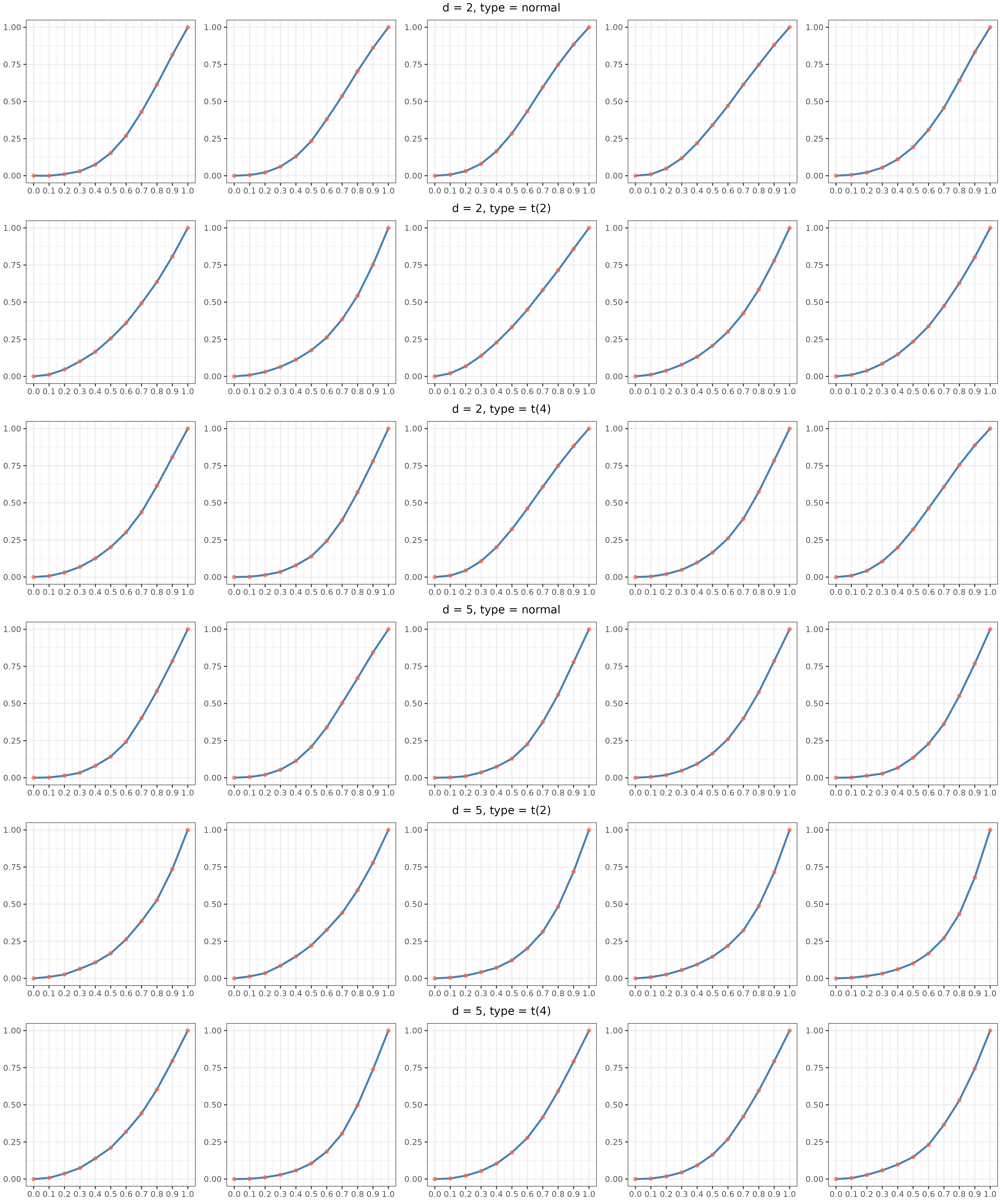
Refer to caption
Figure 2: Values of TACT^{\textrm{AC}} for η\eta between 0 and 11. Here, 𝒁,𝜺\boldsymbol{Z},\boldsymbol{\varepsilon} are generated under various dimensions and distribution types prescribed at the top of each figure. The x-axis of each figure is the value of η\eta; the y-axis is an approximation of TACT^{\textrm{AC}} constructed via 10000001000000 samples. For each specific dimension and distribution type, we plot results for five different randomly generated matrix pairs (B𝒁,B𝜺)(B_{\boldsymbol{Z}},B_{\boldsymbol{\varepsilon}}).