This manuscript was compiled on November 30, 2025\leadauthorSemre et al. \smalltitleQudit Simon’s Algorithm \institutionTechnion \thedayNov 30, 2025
Virtual Qudits for Simon’s Problem: Dimension Lifted Algorithms on Qubit Hardware
Abstract
We study Simon’s problem over the module for arbitrary and show how to explore qudit style advantages using only qubit based hardware and qubit level oracles. Starting from a standard binary () instance with promise oracle , we construct a dimension lifted oracle for by a simple layer wise pack/unpack encoding of qubits into one virtual qudit, and illustrating how qudit style formulations can be studied and exploited on standard qubit devices without access to native multilevel hardware. For a hidden shift of full order , one query to placed between two layers of layer yields measurement outcomes that are exactly uniform on
recovering the original qubit algorithm when . From this structure we derive non-asymptotic bounds on the probability of obtaining independent constraints and obtain explicit repetition budgets as functions of the effective local dimension , showing that the expected number of oracle calls remains while the required repetitions decrease with . Using QuTiP, we simulate these dimension lifted instances (for ), confirming uniform sampling on .
keywords:
Simon’s algorithm, qudits, hidden shift, QFT over , qudit circuits, QuTiP simulation1 Background and Motivation
1.1 From Qubits to Qudits
Quantum computation is most commonly described in terms of qubits, i.e., two level systems with computational basis . At the hardware level, however, many platforms (e.g., trapped ions [Bruzewicz_2019], photonics [Flamini_2018]) naturally exhibit more than two accessible energy levels per physical site. This motivates working with an explicitly multilevel qudit-based based formalism, in which the local Hilbert space is with basis .
Qudits can increase information density [Wang_2020], reduce the depth of certain circuits [Gokhale_2019], and better exploit hardware native transitions [Bruzewicz_2019]. These potential advantages have motivated qudit generalizations of several canonical quantum primitives, including Fourier transforms over [NielsenChuang], multivalued oracles [Muthukrishnan_2000], and other interference based routines [Wang_2020] for dimensions .
In this work, the term “qudit” is used in a slightly broader, algorithmic sense. We allow level systems to be either (i) native multilevel hardware, when available, or (ii) virtual qudits obtained by encoding qubits into one effective level system via a simple pack/unpack map. All of our concrete constructions can be implemented using only qubit level operations and a standard binary Simon oracle; the qudit viewpoint is used to reveal how increasing the effective local dimension impacts the behavior of the algorithm.
Notation and assumptions.
Unless stated otherwise we work over the ring with the standard inner product
Vectors in label computational basis states , which may be realized either as native qudit registers or as encoded blocks of qubits.
1.2 Why Generalize Simon’s Algorithm?
Simon’s algorithm [Simon_1994] is one of the earliest examples of an exponential separation between quantum and classical query complexity. Given a function that is -to- with promise for some unknown , the quantum algorithm recovers using oracle queries, whereas any classical randomized algorithm requires exponentially many queries in [Simon_1994].
While multilevel generalizations exist for other algorithms (such as Deutsch–Jozsa [DeutschJozsa_1992] and Grover search [Grover_1997]), a careful qudit formulation of Simon’s algorithm is particularly attractive for two reasons: (i) it makes explicit how higher dimensional interference structures control sampling uniformity over orthogonal subspaces and the number of repetitions needed to obtain independent constraints; and (ii) it offers a clean setting in which to ask whether qudit style advantages (e.g., fewer repetitions for a fixed failure probability) can be explored and quantified even when only qubit hardware and a binary oracle are available.
The present work uses Simon’s problem as a testbed: we first formulate the algorithm over , and then show how such a -ary instance can be implemented and simulated on qubit based devices by encoding groups of qubits into effective qudits.
1.3 Goals and Contributions of This Work
At a high level, our goal is to highlight how increasing the (effective) local dimension affects the behavior of Simon’s algorithm, and to show that these qudit style effects can already be studied on qubit only platforms by a simple encoding construction. More concretely, this work provides:
-
•
A precise formulation of the -to-one promise over with hidden shift and the associated qudit version of Simon’s algorithm, including the characterization of the measurement outcomes as uniform samples from
-
•
A qubit-native construction of a -to-one oracle for using only the original binary Simon oracle . The construction is based on a layerwise pack/unpack encoding of qubits into one effective qudit, and preserves the hidden shift structure in a dimension lifted instance.
-
•
A complexity analysis that bounds the probability of collecting independent samples from and derives explicit repetition counts as a function of the local dimension . The resulting bounds show that the expected number of oracle calls remains , while the number of repetitions required to achieve a target failure probability decreases as grows.
-
•
Numerical case studies and QuTiP simulations for representative dimensions (e.g., ). These simulations empirically confirm uniform sampling on and illustrate the predicted dimension repetition tradeoff.
2 Quantum Gates and Operations for Qudit Based Algorithms
2.1 States
A qudit lives in [NielsenChuang, Wang_2020] with orthonormal basis , . Any pure state has the form
| (1) |
which we identify with a vector in .
2.2 Gates
2.2.1 X gate
For qubits, flips . For qudits, the generalized shift acts by modular addition:
| (2) |
with modulo . In matrix form, is the cyclic permutation matrix:
For ,
Such multi-valued increment operations are standard primitives in qudit logic and appear in the construction of multi-valued controlled gates and oracles [Muthukrishnan_2000].
2.2.2 H gate
The qudit analogue of the Hadamard is the QFT over :
| (3) |
with matrix
For ,
3 Generalized Simon’s Problem over Qudits
Let be -to-one with hidden shift such that
where denotes addition .
3.1 Complexity
3.1.1 Classical complexity
Any classical randomized algorithm requires exponentially many queries in . In particular, observing a collision (which reveals a multiple of ) needs queries by a birthday paradox argument, and fully identifying remains exponential in .
3.1.2 Coset decomposition
Partition into cosets (orbits) of : choose representatives and set , so that all collide under .
3.2 Quantum algorithm
Given the oracle , the algorithm is:
-
1.
Create superposition. Start with and apply to the first register:
-
2.
Apply the oracle:
-
3.
Apply again:
-
4.
Exploit the promise. Group by orbits with representatives and write :
(4) The inner geometric sum equals if and otherwise; thus only survive, giving
-
5.
Measurement. Measuring the first register yields and a linear constraint . Repeating yields independent equations in expected samples.
Remark.
Setting recovers Simon’s original qubit algorithm.
Probability distribution over .
For any fixed ,
confirming uniformity over .
4 Complexity and Dimension Dependence
Let . After independent samples, the span contains at most elements; hence the probability that the next sample is independent satisfies
Therefore
which is exact when is prime (vector space case), and a valid lower bound otherwise. Consequently, for one full run
and after independent runs,
To ensure ,
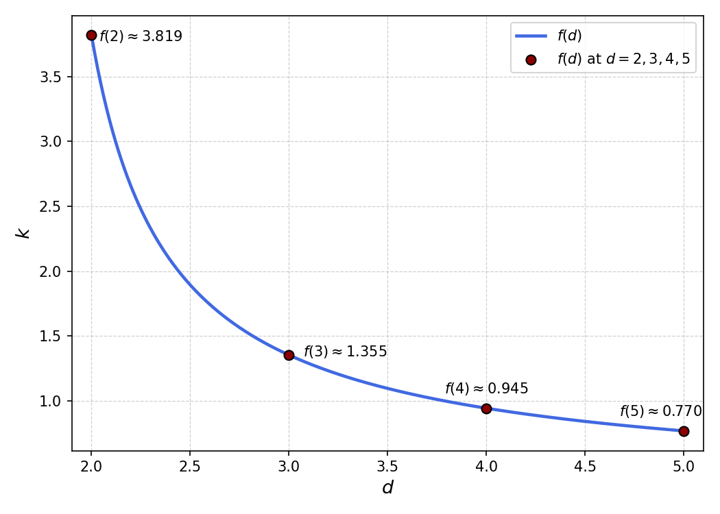
With target failure and large , the base decreases with for , so is monotonically decreasing in . A single shot condition requires, asymptotically,
Illustrative computations for reveal how the admissible region of values shrinks as the error tolerance tightens. Figure 2 summarizes the behavior of across representative levels.


Illustrative thresholds.
Table 1 summarizes the tradeoff between dimension and repetitions for several target failure probabilities. As decreases, the required number of repetitions for qubits grows only logarithmically, while the single shot threshold dimension increases by roughly one order of magnitude for each additional digit of precision.
| Target failure | (i.e., ) | Repetitions |
4.1 Dimensional Lifting via Function Multiplicity Expansion
Beyond the hardware’s native dimension , one may embed a -to-one promise function into a higher dimensional -to-one instance, thereby tightening the single shot failure bound . The resulting bound satisfies
Selecting the smallest integer such that
guarantees one-shot success probability exceeding . Rearranging yields the quadratic condition
This expression quantifies how much the effective dimension must be increased to achieve a given error tolerance. For instance, with and , the bound gives , so suffices, corresponding to and .
5 Simulation of the Qudit Simon Algorithm
We validate the measurement statistics predicted by the qudit variant of Simon’s algorithm by simulating the full unitary circuit in QuTiP. Given local dimension , register size , and hidden shift , the simulation performs: (i) state preparation on two qudit registers, (ii) a generalized Hadamard (QFT) on the first register, (iii) a black box call to for a -to-one promise function with orbits , (iv) projective measurement of the second register to a value in , and (v) a second QFT on the first register followed by measurement.
Minimal pseudocode.
