Generalized discrete Markov spectra

Yasuaki Gyoda Institute for Advanced Research, Nagoya University Furo-cho, Chikusa-ku, Nagoya-shi, 464-8601, Japan ygyoda@math.nagoya-u.ac.jp

Abstract.

We develop a generalized Markov theory for the Markov–Lagrange and Markov spectra. The classical discrete Markov spectrum is governed by Markov numbers, the positive integers occurring in solutions of the Markov equation. We show that this relation admits a cluster-combinatorial extension governed by generalized Markov numbers. Replacing the Christoffel-word formalism by snake graphs, we construct generalized discrete Markov spectra attached to the generalized Markov equations

x^{2}+y^{2}+z^{2}+k_{1}yz+k_{2}zx+k_{3}xy=(3+k_{1}+k_{2}+k_{3})xyz.

Every element of these spectra is realized simultaneously as a Lagrange constant of a quadratic irrational and as a Markov constant of a real indefinite binary quadratic form. We also prove structural results for these spectra, determine their contribution in the transition interval below Freiman’s constant, and identify the boundary value obtained from regular lines of irrational slope, again realizing it both as a Lagrange constant and as a Markov constant.

Key words and phrases:

Markov spectrum, Markov number, Cohn matrix, snake graph

2020 Mathematics Subject Classification:

11J06,11K60,11J70

1. Introduction and Main Results

1.1. Background

The starting point of this paper is the classical link between Diophantine spectra and Markov numbers. We recall it first in a form that will later be generalized by a cluster-combinatorial construction. The Markov spectrum is the set

\mathcal{M}:=\left\{\sup_{(x,y)\in\mathbb{Z}^{2}\setminus\{0\}}\frac{\sqrt{D}}{|Q(x,y)|}\;\middle|\;Q(x,y)=ax^{2}+bxy+cy^{2},\;a,b,c\in\mathbb{R},\;D=b^{2}-4ac>0\right\},

which was studied by Markov around 1880. The Markov constant

\mathcal{M}(Q):=\sup_{(x,y)\in\mathbb{Z}^{2}\setminus\{0\}}\frac{\sqrt{D}}{|Q(x,y)|}

measures, in this setting, how closely the lines defined by the zeros of the quadratic form $Q(x,y)$ approach lattice points. Markov identified the part of the spectrum below $3$ in terms of the integer solutions of a single cubic equation. More precisely, a Markov number is a positive integer that appears in a solution $(x,y,z)\in\mathbb{Z}_{>0}^{3}$ of

x^{2}+y^{2}+z^{2}=3xyz.

Markov proved the following theorem.

Theorem 1.1 (Markov’s theorem [26, 27]).

Let

	$\displaystyle\mathcal{M}_{d}$	$\displaystyle:=\left\{\frac{\sqrt{9n^{2}-4}}{n}\;\middle\|\;n\text{ is a Markov number}\right\}$
	$\displaystyle\mathcal{M}_{<3}$	$\displaystyle:=\{\mathcal{M}(Q)\mid Q:\text{real indefinite quadratic form and }\mathcal{M}(Q)<3\}\subset\mathcal{M}.$

Then $\mathcal{M}_{d}=\mathcal{M}_{<3}$ .

In this paper, we call the set $\mathcal{M}_{d}$ the discrete Markov spectrum. The same set also occurs on the approximation-theoretic side. The Markov–Lagrange spectrum is

\mathcal{L}:=\left\{\limsup_{q\to\infty}\frac{1}{q\|q\alpha\|}\;\middle|\;\alpha\in\mathbb{R}\setminus\mathbb{Q}\right\},

where $\|q\alpha\|$ denotes the distance from $q\alpha$ to the nearest integer. The Lagrange constant

\mathcal{L}(\alpha):=\limsup_{q\to\infty}\frac{1}{q\|q\alpha\|}

is the supremum of those $L$ for which there exist infinitely many rationals $\frac{p}{q}$ satisfying

\left|\alpha-\frac{p}{q}\right|<\frac{1}{Lq^{2}}.

Thus the Markov–Lagrange spectrum records the best quadratic-order rational approximations to irrational numbers. Hurwitz [23] observed that the part of this spectrum below $3$ coincides with the discrete Markov spectrum, namely

\mathcal{L}_{<3}=\mathcal{M}_{<3}=\mathcal{M}_{d}.

This coincidence is the classical bridge between Markov numbers, binary quadratic forms, and Diophantine approximation.

The regions of $\mathcal{L}$ and $\mathcal{M}$ above $3$ are also central objects in the classical theory. Both spectra decompose into three regions: the discrete region below $3$ , governed by Markov numbers; the transition interval $[3,c_{F})$ ; and the continuous region above Freiman’s constant $c_{F}$ , called Hall’s ray, where

c_{F}:=\dfrac{2221564096+283748\sqrt{462}}{491993569}\approx 4.5278295661\dots.

Hall first proved that the spectra contain a half-line, and Freiman later determined the precise beginning of Hall’s ray, namely the above value $c_{F}$ [25, 16, 17]. Outside the transition interval the Markov–Lagrange spectrum and the Markov spectrum coincide completely. Freiman also proved that the two spectra are not equal by constructing Markov constants that are not Lagrange constants [15]. Since the spectra coincide outside the transition interval, this gives the strict inclusion

\mathcal{L}\cap[3,c_{F})\subsetneq\mathcal{M}\cap[3,c_{F}).

For further historical background, see [1, 13, 31].

1.2. Main Results

The aim of this paper is to show that the classical bridge just recalled is not an isolated phenomenon. We develop a generalized Markov theory in which generalized Markov numbers produce explicit Lagrange constants and Markov constants. The construction is governed by the $(k_{1},k_{2},k_{3})$ -generalized Markov (GM) equation

x^{2}+y^{2}+z^{2}+k_{1}yz+k_{2}zx+k_{3}xy=(3+k_{1}+k_{2}+k_{3})xyz,

where $k_{1},k_{2},k_{3}$ are nonnegative integers. A positive integer that appears in a solution to this equation is called a $(k_{1},k_{2},k_{3})$ -generalized Markov number, or $(k_{1},k_{2},k_{3})$ -GM number for short. This equation was introduced by [22, 4] for the case $k_{1}=k_{2}=k_{3}=1$ and by [21] for the general case in the context of generalized cluster algebras. It has since been studied from several perspectives as a Markov-type Diophantine equation (for example, [5, 3, 2, 12, 14, 19, 11, 6, 10]).

Our first main result is a spectral realization theorem. It is the generalized counterpart of the inclusion $\mathcal{M}_{d}\subset\mathcal{M}_{<3}(\subset\mathcal{L})$ in Markov’s theorem and is the basic mechanism from which the generalized discrete Markov spectra are defined.

Theorem 1.2 (Theorem 6.1, Corollaries 6.3, 6.6).

Fix $(k_{1},k_{2},k_{3})\in\mathbb{Z}_{\geq 0}^{3}$ . Let $n$ be a $(k_{1},k_{2},k_{3})$ -GM number, and let $i\in\{1,2,3\}$ be the position of $n$ in a positive integer solution to the $(k_{1},k_{2},k_{3})$ -GM equation. Set

\Delta(n,i):=((3+k_{1}+k_{2}+k_{3})n-k_{i})^{2}-4.

Then there exists a quadratic irrational $\alpha\in\mathbb{Q}(\sqrt{\Delta(n,i)})$ and the corresponding quadratic form $Q=(x-\alpha y)(x-\alpha^{\prime}y)$ , where $\alpha^{\prime}$ is the quadratic conjugate of $\alpha$ , such that

\mathcal{L}(\alpha)=\mathcal{M}(Q)=\dfrac{\sqrt{\Delta(n,i)}}{n}.

In particular, for any $(k_{1},k_{2},k_{3})\in\mathbb{Z}_{\geq 0}^{3}$ ,

\mathcal{M}_{k_{1},k_{2},k_{3}}=\left\{\frac{\sqrt{\Delta(n,i)}}{n}\;\middle|\;\begin{aligned} &\text{the number $n$ is a $(k_{1},k_{2},k_{3})$-GM number, and}\\ &i\text{ is the position of $n$ in a positive integer solution to}\\ &\text{the $(k_{1},k_{2},k_{3})$-GM equation}\end{aligned}\right\}

is contained in both $\mathcal{L}$ and $\mathcal{M}$ .

For $(k_{1},k_{2},k_{3})=(0,0,0)$ this recovers $\mathcal{M}_{d}$ , that is, $\mathcal{M}_{d}=\mathcal{M}_{0,0,0}$ . We therefore call $\mathcal{M}_{k_{1},k_{2},k_{3}}$ the $(k_{1},k_{2},k_{3})$ -generalized discrete Markov spectrum.

The proof is constructive. We attach sign rules to rational-slope lines in the plane; the resulting triangle-crossing and edge-crossing data produce a periodic sequence of positive integers, and the corresponding periodic continued fraction gives the quadratic irrational $\alpha$ in Theorem 1.2. The generalized Markov numbers are realized, at the same time, as numbers of perfect matchings of snake graphs. This planar model is the central combinatorial object of the paper and is also the bridge to the irrational-slope boundary theorem below.

This construction is essential for the generalization. Classical treatments of Markov’s theorem often use Christoffel words (also called Cohn words); see, for instance, [1], [7], and [31]. In that setting, Cohn matrices and strongly admissible sequences can both be read from Christoffel words, and this gives an efficient one-dimensional coding of the classical theory.

The generalized setting requires more information. The generalized Cohn matrices and the generalized strongly admissible sequences do not arise from Christoffel words by the classical construction. The snake-graph model supplies the missing planar data. In this sense, the replacement of Christoffel words by snake graphs is not merely a change of language; it is the mechanism that allows the Markov-number/Diophantine-spectrum correspondence to extend beyond the classical equation. It also gives a new proof-theoretic viewpoint on the classical case.

Markov’s theorem characterizes the classical discrete Markov spectrum as the part of the Markov spectrum below $3$ . The generalized spectra constructed here therefore lead naturally to the following problem.

Question 1.3 (Question 6.12).

Is there a characterization of $\mathcal{M}_{k_{1},k_{2},k_{3}}$ , or of their union, that generalizes Markov’s theorem?

The next results show that these generalized spectra have their own internal structure and are not simply formal shadows of the classical spectrum. The first result relates the classical discrete Markov spectrum to the $(2,2,2)$ -generalized discrete Markov spectrum. It was shown in [21] that classical Markov numbers and $(2,2,2)$ -GM numbers are connected through a remarkable relation involving squaring and taking square roots. We prove the corresponding relation at the spectral level.

Theorem 1.4 (Theorem 6.9).

If $r\in\mathcal{M}_{0,0,0}$ , then $3r\in\mathcal{M}_{2,2,2}$ . Conversely, if $R\in\mathcal{M}_{2,2,2}$ , then $\frac{R}{3}\in\mathcal{M}_{0,0,0}$ .

We also determine exactly which generalized discrete Markov constants lie in the classical transition interval below Freiman’s constant.

Theorem 1.5 (Theorem 6.10).

Set

\mathcal{M}^{\prime}:=\bigcup_{(k_{1},k_{2},k_{3})\in\mathbb{Z}_{\geq 0}^{3}}\mathcal{M}_{k_{1},k_{2},k_{3}}.

Then we have

\mathcal{M}^{\prime}\cap[3,c_{F})=(\mathcal{M}_{0,0,1}\setminus\{\sqrt{5}\})\cup\{2\sqrt{5}\}.

The realization of the numbers in $(\mathcal{M}_{0,0,1}\setminus\{\sqrt{5}\})\cup\{2\sqrt{5}\}$ , especially those with large numbers, both as Lagrange constants and as Markov constants appears to be new. At the same time, other Lagrange constants occur in the transition interval; in particular,

\mathcal{M}^{\prime}\cap[3,c_{F})\subsetneq\mathcal{L}\cap[3,c_{F}).

See Remark 6.11.

The final main result passes from rational slopes to irrational slopes. It identifies the boundary value approached by the rational-slope construction and realizes this value simultaneously on the Lagrange and Markov sides. For a bi-infinite positive integer sequence $\mathbf{a}$ , let $L(\mathbf{a})$ denote the two-sided continued-fraction value defined in Section 2.

Theorem 1.6 (Theorem 6.14, Lemma 6.18, Corollaries 6.20, 6.21).

Fix $(k_{1},k_{2},k_{3})\in\mathbb{Z}_{\geq 0}^{3}$ and $\sigma\in\mathfrak{S}_{3}$ , and put

K=3+k_{1}+k_{2}+k_{3}.

Let $l$ be a regular line of positive irrational slope. Applying the triangle-crossing and edge-crossing sign rules along $l$ , and then recording the lengths of consecutive runs of equal signs, we obtain a bi-infinite positive integer sequence

\mathbf{b}(l)=(b_{n})_{n\in\mathbb{Z}},

where the origin of the index is chosen arbitrarily. For every $r\in\mathbb{Z}$ , set

\alpha_{r}=[b_{r};b_{r+1},b_{r+2},\ldots],\qquad\beta_{r}=-[0;b_{r-1},b_{r-2},\ldots],

and define the real indefinite quadratic form

Q_{r}(x,y)=(x-\alpha_{r}y)(x-\beta_{r}y).

Then for every $r\in\mathbb{Z}$ , we have

L(\mathbf{b}(l))=\mathcal{L}(\alpha_{r})=\mathcal{M}(Q_{r})=K.

In particular, $K\in\mathcal{L}\cap\mathcal{M}$ .

We end by formulating a uniqueness problem suggested by the spectral construction. The classical starting point is Frobenius’s uniqueness conjecture.

Conjecture 1.7 (Conjecture 7.1).

For any Markov number $c$ , there exists a unique Markov triple $(a,b,c)$ such that $a\leq b\leq c$ .

A direct extension to GM numbers leads to the following question.

Question 1.8 (Question 7.3).

For any $(k_{1},k_{2},k_{3})$ -GM number $c$ , is there a unique $(k_{1},k_{2},k_{3})$ -GM triple $(a,b,c)$ such that $a\leq b\leq c$ ?

However, this direct question has already been answered in the negative by [21]. Motivated by the spectral realization theorem above, we instead formulate a generalized version of an equivalent form of the uniqueness conjecture; no counterexample to this formulation is currently known (Conjecture 7.6).

1.3. Organization

Section 2 reviews the classical discrete Markov spectrum and isolates the role played by admissible sequences and Cohn matrices. It also compares the usual Christoffel-word construction with the planar construction used in this paper. Section 3 introduces the generalized Markov equation and generalized Markov numbers. Section 4 constructs generalized Cohn matrices and their matrix factorizations. Section 5 develops generalized Markov length and generalized Markov distance, the main tools in the proof of Theorem 1.2. Section 6 proves the spectral realization theorem, establishes the structural results above, and treats the irrational-slope boundary value and its realizations as Lagrange constants and Markov constants. Section 7 proposes a generalized form of the uniqueness conjecture.

Acknowledgements

The author is deeply grateful to Esther Banaian for communicating Theorem 5.7 and many valuable comments. The author would like to thank the participants of the Markov’s Theorem Seminar at the University of Tsukuba from January 27 to 31, 2025: Kota Saito, Hajime Kaneko, Tadahisa Hamada, Katsuki Ito, Satoru Oshima, and Takafumi Tsurumaki. Special thanks are due to Toshiki Matsusaka and Shigeki Akiyama for their valuable comments. This work was supported by JSPS KAKENHI Grant Number JP25K17224.

2. Classical Discrete Markov Spectrum

This section recalls several well-known facts about the classical Markov spectrum and reformulates them in a way that is compatible with the generalized theory developed later.

2.1. Markov Numbers and Markov Tree

We consider the Markov equation

x^{2}+y^{2}+z^{2}=3xyz.

A positive integer solution of the Markov equation is called a Markov triple, and a positive integer that appears in a Markov triple is a Markov number. We consider the following binary tree $\mathrm{M}\mathbb{T}$ :

(1)

The root vertex is $(1,2,1)$ .
(2)

For a vertex $(a,b,c)$ , its two children are defined as

This tree is called the Markov tree. The first few vertices in $\mathrm{M}\mathbb{T}$ are as follows:

The Markov tree has the following standard properties.

Proposition 2.1 ([19]*Proposition 3.2).

The following statements hold:

(1)

Each vertex $(a,b,c)$ in $\mathrm{M}\mathbb{T}$ is a Markov triple with $b>\max\{a,c\}$ .
(2)

Every Markov triple $(a,b,c)$ with $b>\max\{a,c\}$ appears exactly once in $\mathrm{M}\mathbb{T}$ .

Markov triples also satisfy the following coprimality property.

Proposition 2.2 ([1]*Corollary 3.4).

For any Markov triple $(a,b,c)$ , every pair among $a,b,c$ is relatively prime.

We next introduce the fraction labeling of Markov numbers. For this purpose, we recall Farey triples and the Farey tree, beginning with irreducible fractions in $\mathbb{Q}_{\geq 0}\cup\{\infty\}$ .

Definition 2.3.

Let $q\in\mathbb{Q}_{\geq 0}\cup\{\infty\}$ and $n$ and $d\in\mathbb{Z}_{\geq 0}$ . The symbol $\frac{n}{d}$ is called the reduced expression of $q$ if $n$ and $d$ are relatively prime and $q=\frac{n}{d}$ , where $\frac{n}{d}$ is regarded as $\infty$ when $d=0$ and $n>0$ . A fraction $\frac{n}{d}$ is called irreducible if it is the reduced expression of some $q\in\mathbb{Q}_{\geq 0}\cup\{\infty\}$ .

Definition 2.4.

For $\frac{a}{b}$ and $\frac{c}{d}$ , we denote $ad-bc$ by $\det\!\left(\frac{a}{b},\frac{c}{d}\right)$ . A triple $\left(\frac{a}{b},\frac{c}{d},\frac{e}{f}\right)$ is called a Farey triple if

(1)

$\frac{a}{b},\frac{c}{d},\frac{e}{f}$ are irreducible fractions, and
(2)

$\left|\det\!\left(\frac{a}{b},\frac{c}{d}\right)\right|=\left|\det\!\left(\frac{c}{d},\frac{e}{f}\right)\right|=\left|\det\!\left(\frac{e}{f},\frac{a}{b}\right)\right|=1$ .

We define the Farey tree $\mathrm{F}\mathbb{T}$ as follows:

(1)

The root vertex is $\left(\frac{0}{1},\frac{1}{1},\frac{1}{0}\right)$ .

(2)

Each vertex $\left(\frac{a}{b},\frac{c}{d},\frac{e}{f}\right)$ has the following two children:

where $\frac{a}{b}\oplus\frac{c}{d}=\frac{a+c}{b+d}$ .

The first few vertices of $\mathrm{F}\mathbb{T}$ are as follows:

Proposition 2.5 ([1]*Section 3.2).

The following hold:

(1)

If $\left(r,t,s\right)$ is a Farey triple, then so are $\left(r,r\oplus t,t\right)$ and $\left(t,t\oplus s,s\right)$ . In particular, every vertex in $\mathrm{F}\mathbb{T}$ is a Farey triple.
(2)

For every irreducible fraction $t\in(0,\infty)$ , there exists a unique Farey triple $F$ in $\mathrm{F}\mathbb{T}$ such that $t$ is the second entry of $F$ .
(3)

For $\left(r,t,s\right)$ in $\mathrm{F}\mathbb{T}$ , the inequalities $r<t<s$ hold.

We define $n_{t}$ to be the Markov number in $\mathrm{M}\mathbb{T}$ that corresponds to the irreducible fraction $t\in[0,\infty]$ at the corresponding position in $\mathrm{F}\mathbb{T}$ .

For any Markov triple $(n_{r},n_{t},n_{s})$ in $\mathrm{M}\mathbb{T}$ , we consider an integer $u_{t}$ satisfying the following conditions:

\begin{cases}n_{r}u_{t}\equiv n_{s}\pmod{n_{t}},\\ 0<u_{t}<n_{t}.\end{cases}

The integer $u_{t}$ is uniquely determined because $n_{r}$ , $n_{t}$ , and $n_{s}$ are pairwise relatively prime (Proposition 2.2). Moreover, $u_{t}$ depends only on $t$ , since $(r,t,s)$ is uniquely determined by $t$ according to Proposition 2.5 (2). In this way, $u_{t}$ is defined for $t\in(0,\infty)$ . We set $u_{\frac{0}{1}}=0$ and $u_{\frac{1}{0}}=1$ . We call $u_{t}$ the characteristic number of $t$ .

Lemma 2.6.

For any irreducible fraction $t\in[0,\infty]$ ,

u_{\frac{1}{t}}=n_{t}-u_{t}.

Lemma 2.6 is essentially proved in [19]*Proposition 7.22 (2) (the case $k=0$ ). Indeed, if $(r,t,s)\in\mathrm{F}\mathbb{T}$ , then $(\frac{1}{s},\frac{1}{t},\frac{1}{r})$ appears in $\mathrm{F}\mathbb{T}$ at the position symmetric to $(r,t,s)$ with respect to the central axis of the tree. Moreover, since $(n_{\frac{1}{s}},n_{\frac{1}{t}},n_{\frac{1}{r}})=(n_{s},n_{t},n_{r})$ , the element $v_{t}^{+}$ in [19] coincides with $u_{\frac{1}{t}}$ .

2.2. Cohn Words, Cohn Matrices, and Cohn Tree

Let $\mathfrak{M}_{3}$ be the free (non-commutative) monoid of rank $3$ generated by $\{p,q,r\}$ . We consider the following tree, whose vertices are $\mathfrak{M}_{3}^{3}$ :

(1)

The root vertex is $(p,q,r)\in\mathfrak{M}_{3}^{3}$ .
(2)

For a vertex $(a,b,c)$ , its two children are defined as

This tree is called the Cohn word tree, and we denote it by $\mathrm{CoW}\mathbb{T}$ . We call the word of an element in $\mathfrak{M}_{3}$ appearing in $\mathrm{CoW}\mathbb{T}$ a Cohn word.

The first few Cohn words in $\mathrm{CoW}\mathbb{T}$ are as follows:

\displaystyle\lx@xy@svg{\hbox{\raise 2.5pt\hbox{\kern 18.65508pt\hbox{{\hbox{\kern-18.65508pt\raise 0.0pt\hbox{\hbox{\kern 3.0pt\raise-2.5pt\hbox{$\textstyle{(p,q,r)}$}}}}}{\hbox{\kern 36.23741pt\raise 42.67891pt\hbox{\hbox{\kern 3.0pt\raise-2.5pt\hbox{$\textstyle{\left(q,qr,r\right)}$}}}}}{\hbox{\kern 35.71774pt\raise-42.67891pt\hbox{\hbox{\kern 3.0pt\raise-2.5pt\hbox{$\textstyle{\left(p,pq,q\right)}$}}}}}{\hbox{\kern 102.73117pt\raise 64.01836pt\hbox{\hbox{\kern 3.0pt\raise-2.82002pt\hbox{$\textstyle{\left(qr,qr^{2},r\right)}$}}}}}{\hbox{\kern 102.7144pt\raise 21.33945pt\hbox{\hbox{\kern 3.0pt\raise-2.82002pt\hbox{$\textstyle{\left(q,q^{2}r,qr\right)}$}}}}}{\hbox{\kern 102.19475pt\raise-21.33945pt\hbox{\hbox{\kern 3.0pt\raise-2.82002pt\hbox{$\textstyle{\left(pq,pq^{2},q\right)}$}}}}}{\hbox{\kern 102.09058pt\raise-64.01836pt\hbox{\hbox{\kern 3.0pt\raise-2.82002pt\hbox{$\textstyle{\left(p,p^{2}q,pq\right)}$}}}}}{\hbox{\kern 199.79445pt\raise 74.68808pt\hbox{\hbox{\kern 3.0pt\raise-2.82002pt\hbox{$\textstyle{\left(qr^{2},qr^{3},r\right)}$}}}}}{\hbox{\kern 192.85464pt\raise 53.34863pt\hbox{\hbox{\kern 3.0pt\raise-2.82002pt\hbox{$\textstyle{\left(qr,qrqr^{2},qr^{2}\right)}$}}}}}{\hbox{\kern 193.13242pt\raise 32.00917pt\hbox{\hbox{\kern 3.0pt\raise-2.82002pt\hbox{$\textstyle{\left(q^{2}r,q^{2}rqr,qr\right)}$}}}}}{\hbox{\kern 200.05547pt\raise 10.66972pt\hbox{\hbox{\kern 3.0pt\raise-2.82002pt\hbox{$\textstyle{\left(q,q^{3}r,q^{2}r\right)}$}}}}}{\hbox{\kern 199.5358pt\raise-10.66972pt\hbox{\hbox{\kern 3.0pt\raise-2.82002pt\hbox{$\textstyle{\left(pq^{2},pq^{3},q\right)}$}}}}}{\hbox{\kern 192.0931pt\raise-32.00917pt\hbox{\hbox{\kern 3.0pt\raise-2.82002pt\hbox{$\textstyle{\left(pq,pqpq^{2},pq^{2}\right)}$}}}}}{\hbox{\kern 192.0931pt\raise-53.34863pt\hbox{\hbox{\kern 3.0pt\raise-2.82002pt\hbox{$\textstyle{\left(p^{2}q,p^{2}qpq,pq\right)}$}}}}}{\hbox{\kern 199.43163pt\raise-74.68808pt\hbox{\hbox{\kern 3.0pt\raise-2.82002pt\hbox{$\textstyle{\left(p,p^{3}q,p^{2}q\right)}$}}}}}\ignorespaces\ignorespaces\ignorespaces\ignorespaces{}\ignorespaces\ignorespaces\ignorespaces{\hbox{\lx@xy@drawline@}}\ignorespaces{}\ignorespaces\ignorespaces\ignorespaces{\hbox{\lx@xy@drawline@}}\ignorespaces{\hbox{\lx@xy@drawline@}}\ignorespaces\ignorespaces\ignorespaces\ignorespaces\ignorespaces{}\ignorespaces\ignorespaces\ignorespaces{\hbox{\lx@xy@drawline@}}\ignorespaces{}\ignorespaces\ignorespaces\ignorespaces{\hbox{\lx@xy@drawline@}}\ignorespaces{\hbox{\lx@xy@drawline@}}\ignorespaces\ignorespaces\ignorespaces\ignorespaces\ignorespaces{}\ignorespaces\ignorespaces\ignorespaces{\hbox{\lx@xy@drawline@}}\ignorespaces{}\ignorespaces\ignorespaces\ignorespaces{\hbox{\lx@xy@drawline@}}\ignorespaces{\hbox{\lx@xy@drawline@}}\ignorespaces\ignorespaces\ignorespaces\ignorespaces\ignorespaces{}\ignorespaces\ignorespaces\ignorespaces{\hbox{\lx@xy@drawline@}}\ignorespaces{}\ignorespaces\ignorespaces\ignorespaces{\hbox{\lx@xy@drawline@}}\ignorespaces{\hbox{\lx@xy@drawline@}}\ignorespaces\ignorespaces\ignorespaces\ignorespaces\ignorespaces{}\ignorespaces\ignorespaces\ignorespaces{\hbox{\lx@xy@drawline@}}\ignorespaces{}\ignorespaces\ignorespaces\ignorespaces{\hbox{\lx@xy@drawline@}}\ignorespaces{\hbox{\lx@xy@drawline@}}\ignorespaces\ignorespaces\ignorespaces\ignorespaces\ignorespaces{}\ignorespaces\ignorespaces\ignorespaces{\hbox{\lx@xy@drawline@}}\ignorespaces{}\ignorespaces\ignorespaces\ignorespaces{\hbox{\lx@xy@drawline@}}\ignorespaces{\hbox{\lx@xy@drawline@}}\ignorespaces\ignorespaces\ignorespaces\ignorespaces\ignorespaces{}\ignorespaces\ignorespaces\ignorespaces\ignorespaces{}\ignorespaces\ignorespaces\ignorespaces{\hbox{\lx@xy@drawline@}}\ignorespaces\ignorespaces\ignorespaces\ignorespaces\ignorespaces\ignorespaces{}\ignorespaces\ignorespaces\ignorespaces{\hbox{\lx@xy@drawline@}}\ignorespaces{}\ignorespaces\ignorespaces\ignorespaces{\hbox{\lx@xy@drawline@}}\ignorespaces{\hbox{\lx@xy@drawline@}}\ignorespaces\ignorespaces\ignorespaces\ignorespaces\ignorespaces{}\ignorespaces\ignorespaces\ignorespaces\ignorespaces{}\ignorespaces\ignorespaces\ignorespaces{\hbox{\lx@xy@drawline@}}\ignorespaces\ignorespaces\ignorespaces\ignorespaces\ignorespaces\ignorespaces{}\ignorespaces\ignorespaces\ignorespaces{\hbox{\lx@xy@drawline@}}\ignorespaces{}\ignorespaces\ignorespaces\ignorespaces{\hbox{\lx@xy@drawline@}}\ignorespaces{\hbox{\lx@xy@drawline@}}\ignorespaces\ignorespaces\ignorespaces\ignorespaces\ignorespaces{}\ignorespaces\ignorespaces\ignorespaces\ignorespaces{}\ignorespaces\ignorespaces\ignorespaces{\hbox{\lx@xy@drawline@}}\ignorespaces\ignorespaces\ignorespaces\ignorespaces\ignorespaces\ignorespaces{}\ignorespaces\ignorespaces\ignorespaces{\hbox{\lx@xy@drawline@}}\ignorespaces{}\ignorespaces\ignorespaces\ignorespaces{\hbox{\lx@xy@drawline@}}\ignorespaces{\hbox{\lx@xy@drawline@}}\ignorespaces\ignorespaces\ignorespaces\ignorespaces\ignorespaces{}\ignorespaces\ignorespaces\ignorespaces\ignorespaces{}\ignorespaces\ignorespaces\ignorespaces{\hbox{\lx@xy@drawline@}}\ignorespaces\ignorespaces\ignorespaces\ignorespaces\ignorespaces\ignorespaces{}\ignorespaces\ignorespaces\ignorespaces{\hbox{\lx@xy@drawline@}}\ignorespaces{}\ignorespaces\ignorespaces\ignorespaces{\hbox{\lx@xy@drawline@}}\ignorespaces{\hbox{\lx@xy@drawline@}}\ignorespaces}}}}.

We now recall the geometric realization of Cohn words. For each irreducible fraction $t\in[0,\infty]$ , let $c(t)$ denote the element of $\mathfrak{M}_{3}$ in $\mathrm{CoW}\mathbb{T}$ that corresponds to the position of $t$ in $\mathrm{F}\mathbb{T}$ . In what follows, we shall introduce a geometric construction of $c(t)$ .

We define a word $c_{t}$ associated with a positive irreducible fraction $t$ as follows. Let $t=\frac{a}{b}\in[0,\infty]$ be an irreducible fraction. Consider the line segment in $\mathbb{R}^{2}$ from $(0,0)$ to $(b,a)$ , and denote it by $L_{t}$ . We give $L_{t}$ the orientation from $(0,0)$ to $(b,a)$ . Each time $L_{t}$ intersects a line of the integer lattice, we take the lattice point lying immediately to the right of the intersection point (with respect to the orientation of $L_{t}$ ), and record these in order as $p_{1},p_{2},\dots,p_{n}$ . Here we set $p_{1}=(0,0)$ and $p_{n}=(b,a)$ . If the same lattice point appears more than once, we discard duplicates so that all $p_{i}$ are distinct. Connecting the points $p_{1},p_{2},\dots,p_{n}$ in order by line segments, we assign to each segment a letter according to its slope: - if the slope is $0$ , we assign $p$ ; - if the slope is $1$ , we assign $q$ ; - if the slope is $\infty$ , we assign $r$ .

The sequence of these letters, taken in order, is defined to be $c_{t}$ .

Example 2.7.

The word $c_{\frac{2}{5}}$ is $p^{2}qpq$ , and $c_{\frac{5}{2}}$ is $qrqr^{2}$ . See Figure 1.

Figure 1. The word

c_{\frac{2}{5}}

and

c_{\frac{5}{2}}

Remark 2.8.

The word $c_{t}$ is also known as a Christoffel word.

We use the following standard description of Cohn words.

Theorem 2.9 ([1]*Theorem 7.6).

For any irreducible fraction $t\in[0,\infty]$ , $c_{t}=c(t)$ holds.

Let

P=\begin{bmatrix}3&-1\\ 1&0\end{bmatrix},\quad Q=\begin{bmatrix}5&2\\ 2&1\end{bmatrix},\quad R=\begin{bmatrix}2&1\\ 1&1\end{bmatrix}.

For any irreducible fraction $t\in[0,\infty]$ , we define a matrix $C_{t}$ by

C_{t}:=c_{t}\big|_{p\mapsto P,\ q\mapsto Q,\ r\mapsto R},

and call it a Cohn matrix. We define the Cohn tree $\mathrm{Co}\mathbb{T}$ by

\mathrm{Co}\mathbb{T}:=\mathrm{CoW}\mathbb{T}\big|_{(c_{r},c_{t},c_{s})\mapsto(C_{r},C_{t},C_{s})}.

Remark 2.10.

The Cohn matrix defined here differs from that in [1] in the arrangement of its entries. More precisely, the present definition is obtained from the one in [1] by swapping the diagonal entries.

The first few vertices in $\mathrm{Co}\mathbb{T}$ are as follows:

Theorem 2.11.

For any irreducible fraction $t\in[0,\infty]$ , we have

C_{t}=\begin{bmatrix}3n_{t}-u_{t}&\dfrac{3u_{t}n_{t}-u_{t}^{2}-1}{n_{t}}\\[6.0pt] n_{t}&u_{t}\end{bmatrix}.

In particular, we have $\det(C_{t})=1$ and $\mathrm{tr}(C_{t})=3n_{t}$ .

A proof of Theorem 2.11 can be found in [1]*Theorem 4.13. In [1], only the case $t\in[0,1]$ is treated, but the same argument applies to $t\in(1,\infty]$ as well.

2.3. Continued Fraction Matrix Decompositions of Cohn Matrices

In this subsection, we decompose a Cohn matrix into a product of fundamental matrices using geometric information. We consider the square lattice in $\mathbb{R}^{2}$ (including its grid lines), subdivided by lines of slope $-1$ that pass through lattice points. We denote this modified lattice by $\widetilde{\mathbb{R}^{2}}$ .

For a given irreducible fraction $t=\frac{a}{b}\in(0,\infty)$ , consider again the line segment in $\widetilde{\mathbb{R}^{2}}$ from $(0,0)$ to $(b,a)$ , denoted $L_{t}$ .

Refer to caption — Figure 2. The line segment $L_{t}$ for $t=\frac{2}{5}$

We now define $\overline{L_{t}}$ to be the line segment obtained by shifting $L_{t}$ slightly to the left. We regard that the left endpoint passes through the lower-left edge, whereas the right endpoint remains within the upper-right edge (although the subtle difference in how we treat the two endpoints is not very important in this section, it becomes significant in Section 4 when we assign signs to edges in $\widetilde{\mathbb{R}^{2}}$ ). In Figure 3, the situation described above is illustrated in a deformed manner for better visual clarity. The same type of deformation is used in all subsequent figures.

Remark 2.12.

One can also obtain $\overline{L_{t}}$ using a once-punctured torus: project $L_{t}$ onto an arc on the triangulated once-punctured torus, slightly push the arc upward to obtain a loop, and view $\overline{L_{t}}$ as the embedding of that loop back into $\widetilde{\mathbb{R}^{2}}$ . Figure 4 shows the case where $t=\frac{1}{1}$ .

We use $\overline{L_{t}}$ to construct an integer sequence for any irreducible fraction $t\in(0,\infty)$ . For this purpose, we introduce the sign rule of triangles in $\widetilde{\mathbb{R}^{2}}$ associated with a curve segment.

Let $\gamma$ be a curve segment on $\widetilde{\mathbb{R}^{2}}$ . Here a curve segment $\gamma$ is assumed to satisfy the following conditions:

•

the interior of $\gamma$ does not intersect any lattice point of $\widetilde{\mathbb{R}^{2}}$ ;
•

whenever $\gamma$ meets an edge of $\widetilde{\mathbb{R}^{2}}$ , it intersects the edge transversely;
•

$\gamma$ has only finitely many self-intersections.

Definition 2.13.

Let $\gamma$ be an oriented curve segment on $\widetilde{\mathbb{R}^{2}}$ . For each triangle in $\widetilde{\mathbb{R}^{2}}$ that intersects $\gamma$ , assign a sign in $\{+,-\}$ as follows:

(i)

Assign a sign $(-)$ to each triangle whose left-hand piece, obtained by cutting it with $\gamma$ , is a quadrilateral (see Figure 5):

Figure 5. Right-angled triangles with $-$
(ii)

Assign a sign $(+)$ to all other triangles (see Figure 6):

Figure 6. Right-angled triangles with $+$

This rule is called the triangle-crossing rule of $\gamma$ .

Next, we define the strongly admissible sequence $s(t)$ ¹¹1In [1], the term “strongly admissible sequence” is used for the bi-infinite sequence ${}^{\infty}s(t)^{\infty}$ in the sense of this paper, whereas here we use this name for its single block $s(t)$ . . For $t=\frac{0}{1}$ or $t=\frac{1}{0}$ , set $s(\frac{0}{1})=s(\frac{1}{0})=(1,1)$ . For $t\in(0,\infty)$ , we define $s(t)$ as follows:

(1)

Set the orientation of $\overline{L_{t}}$ from left to right, and arrange the signs assigned to triangles by the triangle-crossing rule in the order in which $\overline{L_{t}}$ intersects them.
(2)

Construct a sequence of integers $(a_{1},\dots,a_{\ell})$ from the counts of consecutive occurrences of the same sign in the sequence from (1). This sequence is called the strongly admissible sequence associated with $t$ , denoted $s(t)$ .

Example 2.14.

Let $t=\frac{2}{5}$ . From Figure 7, the sign sequence is

(-,-,+,-,+,-,+,+,-,-,+,-,+,+),

and therefore

s(\tfrac{2}{5})=(2,1,1,1,1,2,2,1,1,2).

Similarly, for $t=\frac{3}{2}$ , Figure 8 shows the sign sequence

(-,-,+,+,-,-,+,+,-,+),

so that

s(\tfrac{3}{2})=(2,2,2,2,1,1).

Remark 2.15.

We note the following facts.

(1)

If $t\in[1,\infty]$ , then $c_{t}$ consists of letters $q$ and $r$ , and $s(t)$ is obtained from $c_{t}$ by replacing each $q$ with “ $2,2$ ” and each $r$ with “ $1,1$ ”. In [1, 7], $s(t)$ is constructed from $c_{t}$ using this replacement.
(2)

If $t\in(1,\infty)$ , $s(t)$ has the form $(2,2,a_{3},\dots,a_{n-3},1,1)$ . Moreover, in this case,

$s\left(\tfrac{1}{t}\right)=(2,1,1,a_{3},\dots,a_{n-3},2).$

For $a\in\mathbb{Z}_{\geq 1}$ , the matrix $\begin{bmatrix}a&1\\ 1&0\end{bmatrix}$ is called a continued fraction matrix. For any finite integer sequence $S$ , define $CF_{S}$ as the matrix product obtained by substituting each $a\in S$ with the corresponding continued fraction matrix. The following theorem shows that each Cohn matrix decomposes into continued fraction matrices.

Theorem 2.16.

For any irreducible fraction $t\in(0,\infty]$ , we have

C_{t}=CF_{s(t)}.

Proof of Theorem 2.16 for $t\in[1,\infty]$ .

Since

Q=\begin{bmatrix}5&2\\ 2&1\end{bmatrix}=\begin{bmatrix}2&1\\ 1&0\end{bmatrix}^{2},\quad R=\begin{bmatrix}2&1\\ 1&1\end{bmatrix}=\begin{bmatrix}1&1\\ 1&0\end{bmatrix}^{2},

and using Remark 2.15 (1), the theorem follows. ∎

We now consider the case $t\in(0,1)$ .

Lemma 2.17.

For any irreducible fraction $t\in(1,\infty)$ ,

CF_{s(\frac{1}{t})}=\begin{bmatrix}2n_{t}+u_{t}&\dfrac{2n_{t}^{2}-n_{t}u_{t}-u_{t}^{2}-1}{n_{t}}\\ n_{t}&n_{t}-u_{t}\end{bmatrix}.

Proof.

By Remark 2.15 (2), $s(\frac{1}{t})$ is obtained from $s(t)$ by replacing the initial $2,2$ with $2,1,1$ and the final $1,1$ with $2$ . The lemma follows from direct matrix computation (see also [8]*Corollary 24). ∎

Proof of Theorem 2.16 for $t\in(0,1)$ .

By Theorem 2.11 and Lemmas 2.17 and 2.6, the $(2,1)$ - and $(2,2)$ -entries of $C_{t}$ and $CF_{s(t)}$ coincide. Since $\det(C_{t})=\det(CF_{s(t)})=1$ and $\mathrm{tr}(C_{t})=\mathrm{tr}(CF_{s(t)})=3n_{t}$ , the claim follows. ∎

Remark 2.18.

The proof of Theorem 2.16 uses the correspondence between the Cohn (Christoffel) word $c_{t}$ and the strongly admissible sequence $s(t)$ . In Section 4, we give another proof in a more general framework.

2.4. Markov–Lagrange Spectrum and Markov Spectrum

This section recalls the parts of the Markov–Lagrange spectrum and the Markov spectrum needed later. We first recall the Lagrange constant of an irrational number.

Definition 2.19.

For $\alpha\in\mathbb{R}\setminus\mathbb{Q}$ , define the Lagrange constant of $\alpha$ by

\mathcal{L}(\alpha):=\limsup_{q\to\infty}\frac{1}{q\|q\alpha\|}\in\mathbb{R}\cup\{+\infty\},

where $\|q\alpha\|$ denotes the distance from $q\alpha$ to the nearest integer. Equivalently, $\mathcal{L}(\alpha)$ is the supremum of the real numbers $L$ for which

\left|\alpha-\frac{p}{q}\right|<\frac{1}{Lq^{2}}

holds for infinitely many rational numbers $p/q$ . We define

\mathcal{L}:=\{\mathcal{L}(\alpha)\mid\alpha\,\in\,\mathbb{R}\setminus\mathbb{Q}\},

and call it the Markov–Lagrange spectrum.

We recall the Perron identity in a form suited to two-sided continued-fraction sequences. Let $\mathbf{a}=(a_{n})_{n\in\mathbb{Z}}$ be a bi-infinite positive integer sequence. For each $r\in\mathbb{Z}$ , put

\ell_{r}(\mathbf{a}):=[a_{r};a_{r+1},a_{r+2},\ldots]+[0;a_{r-1},a_{r-2},\ldots].

We then set

L(\mathbf{a}):=\sup_{r\in\mathbb{Z}}\ell_{r}(\mathbf{a}).

It is often convenient to specify the cut without referring to an index. If $P=(p_{1},p_{2},\ldots)$ and $Q=(q_{0},q_{1},q_{2},\ldots)$ are right-infinite positive integer sequences, we write $P^{\ast}$ for the sequence $P$ placed to the left of a cut, in the order

P^{\ast}=(\ldots,p_{2},p_{1}),

and define

\ell(P^{\ast}|Q):=[q_{0};q_{1},q_{2},\ldots]+[0;p_{1},p_{2},\ldots].

Thus $\ell(P^{\ast}|Q)$ is the index-free notation for $\ell_{r}(\mathbf{a})$ : when $P=(a_{r-1},a_{r-2},\ldots)$ and $Q=(a_{r},a_{r+1},\ldots)$ , we have

\ell_{r}(\mathbf{a})=\ell(P^{\ast}|Q).

Finally, let $T=(t_{1},\ldots,t_{m})$ be a finite positive integer sequence. We write

T^{\ast}=(t_{m},\ldots,t_{1})

for the reversed sequence, and we use

{}^{\infty}T^{\infty}=\cdots TTT\cdots,\qquad{}^{\infty}T=\cdots TT,\qquad T^{\infty}=TT\cdots

for the periodic extensions. The value $L({}^{\infty}T^{\infty})$ is the maximum of $\ell(P^{\ast}|Q)$ over all cyclic cuts $P^{\ast}|Q$ of the bi-infinite periodic sequence ${}^{\infty}T^{\infty}$ .

The following theorem is the Perron identity for the Markov–Lagrange spectrum.

Theorem 2.20 (Perron identity [29, 30]).

Let $\alpha\in\mathbb{R}\setminus\mathbb{Q}$ , and write its regular continued fraction expansion as

\alpha=[a_{0};a_{1},a_{2},a_{3},\dots],

where $a_{0}\in\mathbb{Z}$ and $a_{i}\in\mathbb{Z}_{>0}$ for $i\geq 1$ . Then

\mathcal{L}(\alpha)=\limsup_{n\to\infty}\left([a_{n+1};a_{n+2},a_{n+3},\dots]+[0;a_{n},a_{n-1},\dots,a_{1}]\right).

In particular, for any finite positive integer sequence $T$ , if $\alpha:=[T^{\infty}]$ , then

\mathcal{L}(\alpha)=L({}^{\infty}T^{\infty}).

Thus, for a periodic continued fraction, the Lagrange constant is obtained by taking the largest cut value of the corresponding bi-infinite periodic sequence.

Next, we introduce the Markov spectrum.

Definition 2.21.

Let $Q(x,y)=ax^{2}+bxy+cy^{2}$ be a real indefinite binary quadratic form, and set $D=b^{2}-4ac$ . We define the Markov constant of $Q$ by

\mathcal{M}(Q):=\sup_{(x,y)\in\mathbb{Z}^{2}\setminus\{0\}}\frac{\sqrt{D}}{|Q(x,y)|}\in\mathbb{R}\cup\{+\infty\},

where this Markov constant is understood to be $+\infty$ if the denominator vanishes for some nonzero lattice point. We define

\mathcal{M}:=\{\mathcal{M}(Q)\mid Q\colon\text{real indefinite binary quadratic form}\},

and call it the Markov spectrum.

The same two-sided continued-fraction notation also gives the quadratic forms appearing in the Perron identity for the Markov spectrum. For a bi-infinite positive integer sequence $\mathbf{a}=(a_{n})_{n\in\mathbb{Z}}$ and $r\in\mathbb{Z}$ , set

\alpha_{r}(\mathbf{a}):=[a_{r};a_{r+1},a_{r+2},\ldots],\qquad\beta_{r}(\mathbf{a}):=-[0;a_{r-1},a_{r-2},\ldots],

and define

Q_{\mathbf{a},r}(x,y):=(x-\alpha_{r}(\mathbf{a})y)(x-\beta_{r}(\mathbf{a})y).

Then

\ell_{r}(\mathbf{a})=\alpha_{r}(\mathbf{a})-\beta_{r}(\mathbf{a}).

For a finite positive integer sequence $T$ , set

\alpha_{T}:=[T^{\infty}],\qquad\beta_{T}:=-[0;(T^{\ast})^{\infty}],\qquad Q_{T}(x,y):=(x-\alpha_{T}y)(x-\beta_{T}y).

Here $\beta_{T}$ is the quadratic conjugate of $\alpha_{T}$ , and hence $Q_{T}$ has rational coefficients.

The following theorem is the Perron identity for the Markov spectrum.

Theorem 2.22 (Perron identity for the Markov spectrum [29, 30]).

Let $\mathbf{a}=(a_{n})_{n\in\mathbb{Z}}\in(\mathbb{Z}_{>0})^{\mathbb{Z}}$ . For every $r\in\mathbb{Z}$ , the Markov constant of the quadratic form $Q_{\mathbf{a},r}$ is

\mathcal{M}(Q_{\mathbf{a},r})=L(\mathbf{a})=\sup_{j\in\mathbb{Z}}\ell_{j}(\mathbf{a}),

where this Markov constant may be $+\infty$ . In particular, for any finite positive integer sequence $T$ , we have

\mathcal{M}(Q_{T})=L({}^{\infty}T^{\infty}).

Thus $\mathcal{L}([T^{\infty}])=\mathcal{M}(Q_{T})=L({}^{\infty}T^{\infty})$ .

When $T$ is a strongly admissible sequence $s(t)$ , the next theorem indicates that this maximizing partition can be explicitly determined.

Theorem 2.23 ([26, 27]).

For any irreducible fraction $t\in[0,\infty]$ ,

(1)

$[s(t)^{\infty}]\in\mathbb{Q}[\sqrt{9n_{t}^{2}-4}]$ , and

(2)

we have

L({}^{\infty}s(t)^{\infty})=\ell(^{\infty}s(t)|s(t)^{\infty})=\ell\left({}^{\infty}s\left(\tfrac{1}{t}\right)\,\middle|\,s\left(\tfrac{1}{t}\right)^{\infty}\right),

and this value is

\frac{\sqrt{9n_{t}^{2}-4}}{n_{t}}.

Here, the value $9n_{t}^{2}=(3n_{t})^{2}$ is determined by the trace of $C_{t}$ . Theorem 2.23 is proved within a more general framework in Section 6. Theorems 2.20, 2.22, and 2.23 immediately imply the following corollary.

Corollary 2.24.

For any strongly admissible sequence $s(t)$ , we have

\mathcal{L}([s(t)^{\infty}])=\mathcal{M}(Q_{s(t)})=\frac{\sqrt{9n_{t}^{2}-4}}{n_{t}}.

We set

\mathcal{M}_{d}:=\left\{\frac{\sqrt{9n^{2}-4}}{n}\ \middle|\ n:\text{Markov number}\right\},

called the discrete Markov spectrum.

There is an important characterization of $\mathcal{M}_{d}$ . Let

	$\displaystyle\mathcal{L}_{<3}$	$\displaystyle:=\{\mathcal{L}(\alpha)\mid\alpha\in\mathbb{R}\setminus\mathbb{Q}\text{ and }\mathcal{L}(\alpha)<3\},$
	$\displaystyle\mathcal{M}_{<3}$	$\displaystyle:=\{\mathcal{M}(Q)\mid Q:\text{real indefinite quadratic form and }\mathcal{M}(Q)<3\}.$

Then by Corollary 2.24 and the fact that $\frac{\sqrt{9n^{2}-4}}{n}<3$ , we have $\mathcal{M}_{d}\subset\mathcal{L}_{<3}$ and $\mathcal{M}_{d}\subset\mathcal{M}_{<3}$ . The converse inclusions also hold.

Theorem 2.25 ([26, 27, 23]).

We have $\mathcal{M}_{d}=\mathcal{L}_{<3}=\mathcal{M}_{<3}$ .

3. Generalized Markov Equation and Generalized Markov Numbers

From this point on, we work with a generalized Markov equation. More precisely, we consider the $(k_{1},k_{2},k_{3})$ -generalized Markov equation

x^{2}+y^{2}+z^{2}+k_{1}yz+k_{2}zx+k_{3}xy=(3+k_{1}+k_{2}+k_{3})xyz,

where $k_{1},k_{2},k_{3}\in\mathbb{Z}_{\geq 0}$ . We abbreviate this equation as the $(k_{1},k_{2},k_{3})$ -GM equation.

A permutation of a positive integer solution to this equation is called a $(k_{1},k_{2},k_{3})$ -GM triple, and a positive integer that appears in some $(k_{1},k_{2},k_{3})$ -GM triple is called a $(k_{1},k_{2},k_{3})$ -GM number. Note that the definition of Markov triples includes all permutations of a solution.

We introduce the $(k_{1},k_{2},k_{3},\sigma)$ -generalized Markov tree (abbreviated $(k_{1},k_{2},k_{3},\sigma)$ -GM tree). Let $\mathfrak{S}_{3}$ be the symmetric group on 3 elements, acting on $\{1,2,3\}$ from the left.

Define the $(k_{1},k_{2},k_{3},\sigma)$ -GM tree $\mathrm{M}\mathbb{T}(k_{1},k_{2},k_{3},\sigma)$ for $\sigma\in\mathfrak{S}_{3}$ as follows:

(1)

The root vertex is

$\big((1,\sigma(1)),(k_{\sigma(2)}+2,\sigma(2)),(1,\sigma(3))\big).$

(2)

Every vertex $((a,h),(b,i),(c,j))$ has the following two children:

Example 3.1.

The first few vertices of $\mathrm{M}\mathbb{T}(1,2,0,\mathrm{id})$ are as follows:

For any $\tau\in\mathfrak{S}_{3}$ , set $\tau(x_{1},x_{2},x_{3}):=(x_{\tau(1)},x_{\tau(2)},x_{\tau(3)})$ . For any $\sigma\in\mathfrak{S}_{3}$ , we denote by $\sigma^{\ast}\in\mathfrak{S}_{3}$ an element satisfying $\sigma(2)=\sigma^{\ast}(2)$ . The following theorem describes all GM triples obtained in this way.

Theorem 3.2.

Let $(a,b,c)$ be a $(k_{1},k_{2},k_{3})$ -GM triple with $b>\max\{a,c\}$ , and assume $\tau(a,b,c)$ is a solution to the $(k_{1},k_{2},k_{3})$ -GM equation for $\tau\in\mathfrak{S}_{3}$ . Then there exists a unique pair $\{\sigma,\sigma^{*}\}\subset\mathfrak{S}_{3}$ and a unique pair $(v,v^{\ast})$ such that $v\in\mathrm{M}\mathbb{T}(k_{1},k_{2},k_{3},\sigma)$ and $v^{\ast}\in\mathrm{M}\mathbb{T}(k_{1},k_{2},k_{3},\sigma^{\ast})$ , and $v$ and $v^{\ast}$ are permutations of $((a,\tau^{-1}(1)),(b,\tau^{-1}(2)),(c,\tau^{-1}(3)))$ . Furthermore, the position of $v^{\ast}$ in $\mathrm{M}\mathbb{T}(k_{1},k_{2},k_{3},\sigma^{\ast})$ is symmetric, with respect to the center, to the position of $v$ in $\mathrm{M}\mathbb{T}(k_{1},k_{2},k_{3},\sigma)$ .

Proof.

It follows from [2]*Proposition 3.8 and [21]*Theorem 1. ∎

In each pair appearing in a vertex of $\mathrm{M}\mathbb{T}(k_{1},k_{2},k_{3},\sigma)$ , the first component is a $(k_{1},k_{2},k_{3})$ -GM number. Moreover, for each triple, the three numbers given by the first components form a solution to the $(k_{1},k_{2},k_{3})$ -GM equation when placed in the positions indicated by the second components of the corresponding pairs. These pairs are called $(k_{1},k_{2},k_{3},\sigma)$ -GM-number-position pairs.

Remark 3.3.

We record the following two facts.

(1)

If $k_{1}=k_{2}=k_{3}$ , then the $(k_{1},k_{2},k_{3},\sigma)$ -GM tree is independent of $\sigma$ up to the position labels. We often omit $\sigma$ in this case.
(2)

If $b=\max\{a,c\}$ , then $(a,b,c)=(1,1,1)$ ([21]*Lemma 4), and therefore the set

$\{v\in\mathrm{M}\mathbb{T}(k_{1},k_{2},k_{3},\sigma)\mid\sigma\in\mathfrak{S}_{3}\}$

contains essentially all $(k_{1},k_{2},k_{3})$ -GM triples except $(1,1,1)$ .

The following proposition generalizes Proposition 2.2.

Proposition 3.4 ([21]*Corollary 8).

For any $(k_{1},k_{2},k_{3})$ -GM triple $(a,b,c)$ , any two of $a,b,c$ are relatively prime.

Now, fix $(k_{1},k_{2},k_{3})\in\mathbb{Z}_{\geq 0}^{3}$ and $\sigma\in\mathfrak{S}_{3}$ .

Abusing notation as in the previous section, we denote by $(n_{t},i_{t})$ the $(k_{1},k_{2},k_{3},\sigma)$ -GM-number-position pair in $\mathrm{M}\mathbb{T}(k_{1},k_{2},k_{3},\sigma)$ located at the position of the irreducible fraction $t\in[0,\infty]$ in $\mathrm{F}\mathbb{T}$ .

For any $(k_{1},k_{2},k_{3})$ -GM triple $(n_{r},n_{t},n_{s})$ in $\mathrm{M}\mathbb{T}(k_{1},k_{2},k_{3},\sigma)$ , consider an integer $u_{t}$ satisfying:

\begin{cases}n_{r}u_{t}\equiv n_{s}\pmod{n_{t}},\\ 0<u_{t}<n_{t}.\end{cases}

The integer $u_{t}$ is uniquely determined since $n_{r},n_{t},n_{s}$ are pairwise relatively prime. Moreover, $u_{t}$ depends only on $t$ , since $(r,t,s)$ is determined by $t$ from Proposition 2.5 (2).

For $t\in(0,\infty)$ , we define $u_{t}$ as above, and set

u_{\frac{0}{1}}=-k_{\sigma(1)},\quad u_{\frac{1}{0}}=1.

The number $u_{t}$ is called the characteristic number of $t$ .

Remark 3.5.

Let $(n^{\ast}_{\frac{1}{t}},i^{*}_{\frac{1}{t}})$ be a $(k_{1},k_{2},k_{3},\sigma^{\ast})$ -GM number-position pair associated with $\frac{1}{t}$ . Then by Theorem 3.2, we have

(n_{t},i_{t})=(n_{\frac{1}{t}}^{\ast},i^{\ast}_{\frac{1}{t}}).

We abbreviate $k_{i_{t}}$ as $k_{t}$ . The following lemma generalizes Lemma 2.6.

Lemma 3.6.

For any irreducible fraction $t\in(0,\infty)$ ,

u^{\ast}_{\frac{1}{t}}=n_{t}-u_{t}-k_{t}.

For $k_{1}=k_{2}=k_{3}$ , Lemma 3.6 is proved in [19]*Proposition 7.22 (2). The general case is proved in the same way. As in the case of Lemma 2.6, replace $v_{t}^{+}$ in [19] with $u^{*}_{\frac{1}{t}}$ .

4. Generalized Cohn Matrices and Their Decompositions

This section introduces analogues of Cohn matrices corresponding to GM numbers and derives their continued-fraction matrix decompositions.

4.1. Generalized Cohn Matrices

Fix $k_{1},k_{2},k_{3}\in\mathbb{Z}_{\geq 0}$ and $\sigma\in\mathfrak{S}_{3}$ . We set

	$\displaystyle C_{\frac{0}{1}}$	$\displaystyle=\begin{bmatrix}3+k_{1}+k_{2}+k_{3}&-(3+k_{1}+k_{2}+k_{3})k_{\sigma(1)}-1\\ 1&-k_{\sigma(1)}\end{bmatrix},$
	$\displaystyle C_{\frac{1}{1}}$	$\displaystyle=\begin{bmatrix}(3+k_{1}+k_{2}+k_{3})(k_{\sigma(2)}+2)-k_{\sigma(2)}-1&2+k_{1}+k_{2}+k_{3}\\ k_{\sigma(2)}+2&1\end{bmatrix},$
	$\displaystyle C_{\frac{1}{0}}$	$\displaystyle=\begin{bmatrix}2+k_{1}+k_{2}+k_{3}-k_{\sigma(3)}&1+k_{1}+k_{2}+k_{3}-k_{\sigma(3)}\\ 1&1\end{bmatrix}.$

For any $(r,t,s)\in\mathrm{F}\mathbb{T}$ , we set inductively

C_{r\oplus t}:=C_{r}C_{t}-D_{s},\quad C_{t\oplus s}=C_{t}C_{s}-D_{r},

where

D_{r}=\begin{bmatrix}k_{r}&k_{r}(3+k_{1}+k_{2}+k_{3})\\ 0&k_{r}\end{bmatrix}.

These matrices coincide with ordinary Cohn matrices when $k_{1}=k_{2}=k_{3}=0$ . The matrix $C_{t}$ is called a $(k_{1},k_{2},k_{3},\sigma)$ -generalized Cohn matrix. Define the $(k_{1},k_{2},k_{3},\sigma)$ -generalized Cohn tree:

\mathrm{Co}\mathbb{T}(k_{1},k_{2},k_{3},\sigma):=\mathrm{F}\mathbb{T}\big|_{(r,t,s)\mapsto(C_{r},C_{t},C_{s})}.

Example 4.1.

The first few vertices in $\mathrm{Co}\mathbb{T}(1,2,0,\mathrm{id})$ are:

Theorem 4.2.

For any irreducible fraction $t\in[0,\infty]$ , we have

C_{t}=\begin{bmatrix}(3+k_{1}+k_{2}+k_{3})n_{t}-k_{t}-u_{t}&\dfrac{(3+k_{1}+k_{2}+k_{3})n_{t}u_{t}-k_{t}u_{t}-u_{t}^{2}-1}{n_{t}}\\ n_{t}&u_{t}\end{bmatrix}.

In particular, we have $\det(C_{t})=1$ and $\mathrm{tr}(C_{t})=(3+k_{1}+k_{2}+k_{3})n_{t}-k_{t}$ .

The case $k_{1}=k_{2}=k_{3}$ and $t\in[0,1]$ is treated in [20]*Lemma 4.5; the same argument proves the general case.

4.2. Continued Fraction Matrix Decompositions of Generalized Cohn Matrices

As in Section 2, we use geometric information to decompose $C_{t}$ into a product of fundamental matrices. For any irreducible fraction $t\in[0,\infty]$ , we construct a generalized strongly admissible sequence $s(t)$ by the triangle-crossing rule introduced in Section 2 and the following edge-crossing rule.

Definition 4.3.

We fix $(k_{1},k_{2},k_{3})\in\mathbb{Z}_{\geq 0}^{3}$ and $\sigma\in\mathfrak{S}_{3}$ . Let $\gamma$ be an oriented curve segment on $\widetilde{\mathbb{R}^{2}}$ . For each edge in a triangle intersecting the interior of $\gamma$ , assign signs as follows:

(i)

Assign $k_{\sigma(1)}$ (resp., $k_{\sigma(2)}$ , $k_{\sigma(3)}$ ) minus signs ( $-$ ) to each horizontal (resp., diagonal, vertical) edge whose midpoint is not strictly on the right side of $\gamma$ (see Figure 9).

Figure 9. Edges with $-$
(ii)

Assign $k_{\sigma(1)}$ (resp., $k_{\sigma(2)}$ , $k_{\sigma(3)}$ ) plus signs ( $+$ ) to each horizontal (resp., diagonal, vertical) edge whose midpoint is on the right side of $\gamma$ (see Figure 10).

Figure 10. Edges with $+$

This rule is called the edge-crossing rule of $\gamma$ for $(k_{1},k_{2},k_{3},\sigma)$ .

Thus, for any such curve segment $\gamma$ , the triangle-crossing and edge-crossing rules assign a finite sequence of signs to $\gamma$ , read in the order in which $\gamma$ passes through the corresponding triangles and edges. For the rational-slope segment $\overline{L_{t}}$ , the generalized strongly admissible sequence $s(t)$ is obtained by recording the lengths of maximal consecutive runs of equal signs.

We define a $(k_{1},k_{2},k_{3},\sigma)$ -generalized strongly admissible sequence $s(t)$ . First, set

s(\tfrac{0}{1})=(1+k_{\sigma(2)}+k_{\sigma(3)},1),\quad s(\tfrac{1}{0})=(1+k_{\sigma(1)}+k_{\sigma(2)},1).

For any irreducible fraction $t\in(0,\infty)$ , we define $s(t)$ as follows:

(1)

Orient $\overline{L_{t}}$ from left to right, and arrange the signs assigned by the triangle-crossing and edge-crossing rules in the order in which $\overline{L}_{t}$ passes through them.
(2)

Construct the integer sequence $(a_{1},\dots,a_{\ell})$ from the lengths of the maximal consecutive runs of equal signs in (1). This sequence is called the generalized strongly admissible sequence associated with $t$ , denoted $s(t)$ .

Example 4.4.

Let $(k_{1},k_{2},k_{3},\sigma)=(1,2,0,\textrm{id})$ and $t=\frac{2}{5}$ . Figure 11 shows the signs along $\overline{L}_{t}$ , giving

s(\tfrac{2}{5})=(5,1,3,3,1,5,4,1,3,4).

The right endpoint of $\overline{L_{t}}$ lies within the upper-rightmost edge in $\widetilde{\mathbb{R}^{2}}$ ; therefore no sign is assigned to this edge. Although the unique horizontal edge intersecting $\overline{L_{t}}$ appears to meet it at its midpoint, in fact, since $\overline{L_{t}}$ is defined by shifting $L_{t}$ slightly to the left, the intersection point lies slightly to the left of the midpoint. Thus the corresponding sign is $+$ .

Remark 4.5.

For $s(t)=(a_{1},\dots,a_{n})$ :

(1)

$a_{1}=2+k_{1}+k_{2}+k_{3}$ .
(2)

If $t=\frac{1}{1}$ , then $s(t)=(2+k_{1}+k_{2}+k_{3},2+k_{\sigma(2)}).$
(3)

If $t\in(0,1)$ , then $a_{2}=1$ , and $a_{n}\neq 1$ . If $t\in(1,\infty)$ , then $a_{2}\neq 1$ , and $a_{n}=1$ .
(4)

If $t=\frac{1}{2}$ , then $n=4$ and $a_{4}=a_{3}+1+k_{t}$ . If $t=\frac{2}{1}$ , then $n=4$ and $a_{2}=a_{3}+1+k_{t}$ .
(5)

If $t\in(0,\frac{1}{2})\cup(\frac{1}{2},1)$ , then $a_{3}+1=a_{n}$ , $a_{3+i}=a_{n-i}$ for $i=1,2,\dots,\frac{n}{2}-3$ . Moreover, we have $a_{\frac{n}{2}+1}=a_{\frac{n}{2}+2}+(-1)^{\frac{n}{2}+1}k_{t}$ .
(6)

If $t\in(1,\frac{2}{1})\cup(\frac{2}{1},\infty)$ , then $a_{2}=a_{n-1}+1$ , $a_{2+i}=a_{n-i-1}$ for $i=1,2,\dots,\frac{n}{2}-3$ . Moreover, we have $a_{\frac{n}{2}}=a_{\frac{n}{2}+1}+(-1)^{\frac{n}{2}}k_{t}$ .
(7)

For $t\in(0,\infty)$ , denote by $s^{\ast}(\frac{1}{t})$ the $(k_{1},k_{2},k_{3},\sigma^{\ast})$ -generalized strongly admissible sequence, expressed as $(a_{1},a_{n},a_{n-1},\dots,a_{2})$ . The bi-infinite sequence ${}^{\infty}(s^{*}(\tfrac{1}{t}))^{\infty}$ is the reverse of ${}^{\infty}s(t)^{\infty}$ . The same statement also holds for $t=\frac{0}{1}$ and $\frac{1}{0}$ .

We prove the following theorem.

Theorem 4.6.

For any irreducible fraction $t\in(0,\infty]$ , we have $C_{t}=CF_{s(t)}$ .

To prove Theorem 4.6, we introduce the snake graph. Assume $a_{i}\in\mathbb{Z}_{\geq 1}$ . First, recall the snake graph associated with a continued fraction $[a_{1},\dots,a_{\ell}]$ according to [9]:

For a continued fraction $[a_{1},\dots,a_{\ell}]$ with $(\ell,a_{1})\neq(1,1)$ :

(1)

Arrange $(a_{1}+\cdots+a_{\ell})$ signs: the first $a_{1}$ are $-$ , the next $a_{2}$ are $+$ , alternating between $-$ and $+$ .
(2)

Remove the first and last signs to obtain a tuple $S$ of length $(a_{1}+\cdots+a_{\ell}-2)$ .
(3)
Using $S$ , place tiles as in Figure 12, satisfying:
- •
  
  The first (leftmost) tile is the left one in Figure 12.
- •
  
  Each new tile is placed to the right or above the preceding tile.
- •
  
  Signs on adjoining edges coincide.
- •
  
  $S$ coincides with the sequence of signs on adjoining parts from left to right.

This graph is the snake graph, denoted $\mathcal{G}[a_{1},\dots,a_{\ell}]$ . For the empty continued fraction $[\ ]$ , set $\mathcal{G}[\ ]=\emptyset$ . For $[1]$ , set $\mathcal{G}[1]$ as a line segment. $\mathcal{G}[2]$ is a single tile.

Example 4.7.

For $[2,4,2,1]$ , the snake graph is shown in Figure 13. Indeed, the signs located inside the connected tiles are arranged from the leftmost to the rightmost as follows: there are ( $2-1$ ) consecutive “ $-$ ” signs, followed by 4 “ $+$ ” signs, then 2 “ $-$ ” signs, and finally $(1-1)$ (therefore, no) consecutive “ $+$ ” signs.

Remark 4.8.

The sign on the right edge in each tile is different from one on the upper edge. Therefore, for a continued fraction $[a_{1},\dots,a_{\ell}]$ , there is a unique snake graph associated with $[a_{1},\dots,a_{\ell}]$ .

Let $G$ be an undirected graph. We recall that a subset $P$ of the edge set of $G$ is called a perfect matching of $G$ if each vertex of $G$ is incident to exactly one edge in $P$ . We denote by $m(\mathcal{G}[a_{1},\dots,a_{\ell}])$ the number of perfect matchings of $\mathcal{G}[a_{1},\dots,a_{\ell}]$ . We set $m(\mathcal{G}[\ ])=1$ .

Example 4.9.

By an induction argument, we have $m(\mathcal{G}[n])=n$ . Figure 14 is the list of perfect matchings of $\mathcal{G}[5]$ .

Figure 14. List of perfect matchings of

\mathcal{G}[5]

The following proposition follows from the fact that the number of perfect matchings of a snake graph is invariant under congruent transformations of the graph.

Proposition 4.10.

For any integer sequence $(a_{1},\dots,a_{n})$ , we have

m(\mathcal{G}[a_{1},\dots,a_{n}])=m(\mathcal{G}[a_{n},\dots,a_{1}]).

In [9], the authors establish the following relation between a continued fraction and its associated snake graph:

Theorem 4.11 ([9]*Theorem 3.4).

The following equality holds:

[a_{1},\dots,a_{n}]=\frac{m(\mathcal{G}[a_{1},\dots,a_{n}])}{m(\mathcal{G}[a_{2},\dots,a_{n}])}.

We note that Theorem 4.11 also covers the case in which the denominator on the right-hand side is $m(\mathcal{G}[\ ])$ .

If $[a_{1},\dots,a_{n}]=\frac{p_{n}}{q_{n}}$ , then the corresponding product of continued fraction matrices is given by (see [7]*Section 2.1):

\begin{bmatrix}a_{1}&1\\ 1&0\end{bmatrix}\begin{bmatrix}a_{2}&1\\ 1&0\end{bmatrix}\cdots\begin{bmatrix}a_{n}&1\\ 1&0\end{bmatrix}=\begin{bmatrix}p_{n}&p_{n-1}\\ q_{n}&q_{n-1}\end{bmatrix}.

By Theorem 4.11, this can be restated as

(4.1)

\displaystyle\begin{bmatrix}a_{1}&1\\ 1&0\end{bmatrix}\begin{bmatrix}a_{2}&1\\ 1&0\end{bmatrix}\cdots\begin{bmatrix}a_{n}&1\\ 1&0\end{bmatrix}=\begin{bmatrix}m(\mathcal{G}[a_{1},\dots,a_{n}])&m(\mathcal{G}[a_{1},\dots,a_{n-1}])\\ m(\mathcal{G}[a_{2},\dots,a_{n}])&m(\mathcal{G}[a_{2},\dots,a_{n-1}])\end{bmatrix}.

Hence, to prove Theorem 4.6, it suffices to show that for $s(t)=(a_{1},\dots,a_{n})$ ,

(4.2)

\displaystyle C_{t}=\begin{bmatrix}m(\mathcal{G}[a_{1},\dots,a_{n}])&m(\mathcal{G}[a_{1},\dots,a_{n-1}])\\ m(\mathcal{G}[a_{2},\dots,a_{n}])&m(\mathcal{G}[a_{2},\dots,a_{n-1}])\end{bmatrix}

for any $t\in(0,\infty]$ .

On the other hand, [19]*Theorem 7.10 provides an expression for $C_{t}$ for $t\in(0,1)$ . In the notation of the present paper, it gives the following theorem.

Theorem 4.12.

Let $t\in(0,1)$ be an irreducible fraction. For $s(t)=(a_{1},\dots,a_{n})$ , we have

(4.3)

\displaystyle C_{t}=\scalebox{0.85}{$\begin{bmatrix}\hskip-28.45274pt(3+k_{1}+k_{2}+k_{3})m(\mathcal{G}[a_{n},\dots,a_{3}+1])&(3+k_{1}+k_{2}+k_{3})m(\mathcal{G}[a_{n-1},\dots,a_{3}+1])\\ \hskip 142.26378pt-m(\mathcal{G}[a_{n},\dots,a_{4}])&\hskip 142.26378pt-m(\mathcal{G}[a_{n-1},\dots,a_{4}])\\ m(\mathcal{G}[a_{n},\dots,a_{3}+1])&m(\mathcal{G}[a_{n-1},\dots,a_{3}+1])\end{bmatrix}$},

Remark 4.13.

Note that when comparing Theorem 4.12 with [19]*Theorem 7.10 (2), the positions of the matrix entries differ due to the difference in the convention of Cohn matrices described in Remark 2.10.

Theorem 4.12 gives the following description of $C_{t}$ for $t\in(1,\infty)$ .

Theorem 4.14.

Let $t\in(1,\infty)$ be an irreducible fraction. For $s(t)=(a_{1},\dots,a_{n})$ , we have

(4.4)

\displaystyle C_{t}=\scalebox{1.0}{$\begin{bmatrix}\hskip-28.45274pt(2+k_{1}+k_{2}+k_{3})m(\mathcal{G}[a_{n},\dots,a_{2}])&\ast\\ \hskip 142.26378pt+m(\mathcal{G}[a_{n},\dots,a_{3}])&\\ m(\mathcal{G}[a_{n},\dots,a_{2}])&m(\mathcal{G}[a_{n-1},\dots,a_{2}])\end{bmatrix}$}

Remark 4.15.

The $(1,2)$ entry in (4.4) is omitted since it does not need to be proved, but it is actually

(2+k_{1}+k_{2}+k_{3})\,m(\mathcal{G}[a_{n-1},\dots,a_{2}])+m(\mathcal{G}[a_{n-1},\dots,a_{3}]).

To prove Theorem 4.14, we need the snake graph calculus. The following two lemmas are essentially proved by [3]. In this paper, the statement is formulated in terms of the numerators of continued fractions, but by applying Theorem 4.11 it can be rephrased as a statement about the number of perfect matchings.

Lemma 4.16 ([3]*Lemma 3).

Let $n\geq 2$ . For any integer sequence $(a_{1},\dots,a_{n})$ , the following equality holds:

m(\mathcal{G}[a_{1},\dots,a_{n}])=a_{n}m(\mathcal{G}[a_{1},\dots,a_{n-1}])+m(\mathcal{G}[a_{1},\dots,a_{n-2}]),

where $m(\mathcal{G}[a_{1},a_{0}])=1$ .

We call a sequence of the form $(a_{1},\dots,a_{\ell-1},\,a_{\ell}+k,\,a_{\ell},\,a_{\ell-1},\dots,a_{1})$ a semi-palindromic sequence, where $k\in\mathbb{Z}$ .

Lemma 4.17.

For any semi-palindromic integer sequence $(a_{1},\dots,a_{\ell-1},a_{\ell}+k,a_{\ell},a_{\ell-1},\dots,a_{1})$ , the following identity holds:

m(\mathcal{G}[a_{2},\dots,a_{\ell-1},a_{\ell}+k,a_{\ell},a_{\ell-1},\dots,a_{1}])=m(\mathcal{G}[a_{1},\dots,a_{\ell-1},a_{\ell}+k,a_{\ell},a_{\ell-1},\dots,a_{2}])+(-1)^{\ell}k.

Moreover, this identity is equivalent to

m(\mathcal{G}[a_{2},\dots,a_{\ell-1},a_{\ell},a_{\ell}+k,a_{\ell-1},\dots,a_{1}])=m(\mathcal{G}[a_{1},\dots,a_{\ell-1},a_{\ell},a_{\ell}+k,a_{\ell-1},\dots,a_{2}])+(-1)^{\ell+1}k.

Proof.

For the first statement of Lemma 4.17, the case $k=1$ is proved in [3]*Lemma 5. The other cases are proved by the same argument. The second statement follows from Proposition 4.10. ∎

We now prove Theorem 4.14.

Proof of Theorem 4.14.

Let $s^{\ast}(\tfrac{1}{t})=(b_{1},\dots,b_{\ell})$ . Since $b_{2}=1$ by Remark 4.5 (3), we have

m(\mathcal{G}[b_{\ell},\dots,b_{3}+1])=m(\mathcal{G}[b_{\ell},\dots,b_{2}]).

By Theorem 4.2 and Theorem 4.12, it follows that

n^{\ast}_{\frac{1}{t}}=m(\mathcal{G}[b_{\ell},\dots,b_{2}]),\quad u^{\ast}_{\frac{1}{t}}=m(\mathcal{G}[b_{\ell-1},\dots,b_{2}]).

Moreover, by Remark 4.5 (7), we have $\ell=n$ , $b_{1}=a_{1}$ , and $b_{i}=a_{n-i+2}$ for $2\leq i\leq n$ . We recall Remark 3.5 and Lemma 3.6, that is,

n_{t}=n^{\ast}_{\frac{1}{t}},\qquad u_{t}=n_{t}-u^{\ast}_{\frac{1}{t}}-k_{t}.

Thus, we have

(4.5)		$\displaystyle n_{t}$	$\displaystyle=m(\mathcal{G}[a_{2},\dots,a_{n}]),$
(4.6)		$\displaystyle u_{t}$	$\displaystyle=m(\mathcal{G}[a_{2},\dots,a_{n}])-m(\mathcal{G}[a_{3},\dots,a_{n}])-k_{t}.$

Since $a_{n}=1$ by Remark 4.5 (3), we obtain

(4.7)

\displaystyle m(\mathcal{G}[a_{3},\dots,a_{n}])=m(\mathcal{G}[a_{3},\dots,a_{n-1}+1]).

Furthermore, since $(a_{2},\dots,a_{n-1}+1)$ is a semi-palindrome by Remark 4.5 (4) and (6), we obtain

(4.8)

\displaystyle m(\mathcal{G}[a_{2},\dots,a_{n-2}])=m(\mathcal{G}[a_{3},\dots,a_{n-1}+1])+k_{t}\stackrel{{\scriptstyle\eqref{eq:a_n=a_n-1+1}}}{{=}}m(\mathcal{G}[a_{3},\dots,a_{n}])+k_{t},

from Lemma 4.17. Therefore, substituting (4.8) into (4.6), we have

u_{t}=m(\mathcal{G}[a_{2},\dots,a_{n}])-m(\mathcal{G}[a_{2},\dots,a_{n-2}]).

Since $a_{n}=1$ again, Lemma 4.16 yields

m(\mathcal{G}[a_{2},\dots,a_{n}])=m(\mathcal{G}[a_{2},\dots,a_{n-1}])+m(\mathcal{G}[a_{2},\dots,a_{n-2}]).

Hence, we conclude that

u_{t}=m(\mathcal{G}[a_{n-1},\dots,a_{2}]).

By Theorem 4.2, it follows that

C_{t}=\begin{bmatrix}\ast&\ast\\ m(\mathcal{G}[a_{n},\dots,a_{2}])&m(\mathcal{G}[a_{n-1},\dots,a_{2}])\end{bmatrix}.

Since $\mathrm{tr}(C_{t})=(3+k_{1}+k_{2}+k_{3})n_{t}-k_{t}$ , using (4.8), the $(1,1)$ -entry is

(2+k_{1}+k_{2}+k_{3})\,m(\mathcal{G}[a_{n},\dots,a_{2}])+m(\mathcal{G}[a_{n},\dots,a_{3}]).

∎

To prove Theorem 4.6, we use one more relation between snake graphs.

Lemma 4.18.

Let $n\geq 4$ . For any sequence $(a_{1},1,a_{3},\dots,a_{n})$ , we have

m(\mathcal{G}[a_{1},1,a_{3},\dots,a_{n}])=(a_{1}+1)m(\mathcal{G}[a_{3}+1,\dots,a_{n}])-m(\mathcal{G}[a_{4},\dots,a_{n}]).

The special case needed in [19] is proved there in equation (7.2), and Lemma 4.18 follows by the same argument.

Proof of Theorem 4.6.

The cases $t=\frac{1}{1}$ and $t=\frac{1}{0}$ can be checked directly. We focus on $t\in(0,1)$ . Comparing (4.2) and (4.3), it suffices to show

(4.9)	$\displaystyle m(\mathcal{G}[a_{1},\dots,a_{n}])$	$\displaystyle=(3+k_{1}+k_{2}+k_{3})m(\mathcal{G}[a_{n},\dots,a_{3}+1])-m(\mathcal{G}[a_{n},\dots,a_{4}]),$
(4.10)	$\displaystyle m(\mathcal{G}[a_{1},\dots,a_{n-1}])$	$\displaystyle=(3+k_{1}+k_{2}+k_{3})m(\mathcal{G}[a_{n-1},\dots,a_{3}+1])-m(\mathcal{G}[a_{n-1},\dots,a_{4}]),$
(4.11)	$\displaystyle m(\mathcal{G}[a_{2},\dots,a_{n}])$	$\displaystyle=m(\mathcal{G}[a_{n},\dots,a_{3}+1]),$
(4.12)	$\displaystyle m(\mathcal{G}[a_{2},\dots,a_{n-1}])$	$\displaystyle=m(\mathcal{G}[a_{n-1},\dots,a_{3}+1]).$

Since $a_{2}=1$ , we have

m(\mathcal{G}[a_{n},\dots,a_{3}+1])=m(\mathcal{G}[a_{n},\dots,a_{2}]),\quad m(\mathcal{G}[a_{n-1},\dots,a_{3}+1])=m(\mathcal{G}[a_{n-1},\dots,a_{2}]).

Since $\mathcal{G}[a_{n},\dots,a_{2}]$ and $\mathcal{G}[a_{2},\dots,a_{n}]$ are mirror images of each other as graphs, the values $m(\mathcal{G}[a_{n},\dots,a_{2}])$ and $m(\mathcal{G}[a_{2},\dots,a_{n}])$ are equal. Therefore, (4.11) and (4.12) hold.

By Remark 4.5 (1), Equation (4.9) can be rewritten as

m(\mathcal{G}[2+k_{1}+k_{2}+k_{3},1,a_{3},\dots,a_{n}])=(3+k_{1}+k_{2}+k_{3})m(\mathcal{G}[a_{n},\dots,a_{3}+1])-m(\mathcal{G}[a_{n},\dots,a_{4}]).

This is the special case $a_{1}=2+k_{1}+k_{2}+k_{3}$ of Lemma 4.18. The proof of (4.10) is identical. It remains to prove the statement for $t\in(1,\infty)$ . Since $\det(CF_{s(t)})=1$ and $\det C_{t}=1$ by Theorem 4.2, it suffices to show the equality of the $(1,1)$ -, $(2,1)$ -, and $(2,2)$ -entries. Comparing (4.2) and (4.4), it suffices to show

(4.13)	$\displaystyle m(\mathcal{G}[a_{1},\dots,a_{n}])$	$\displaystyle=(2+k_{1}+k_{2}+k_{3})m(\mathcal{G}[a_{n},\dots,a_{2}])+m(\mathcal{G}[a_{n},\dots,a_{3}]),$
(4.14)	$\displaystyle m(\mathcal{G}[a_{2},\dots,a_{n}])$	$\displaystyle=m(\mathcal{G}[a_{n},\dots,a_{2}]),$
(4.15)	$\displaystyle m(\mathcal{G}[a_{2},\dots,a_{n-1}])$	$\displaystyle=m(\mathcal{G}[a_{n-1},\dots,a_{2}]).$

The equation (4.13) follows from Lemma 4.16, and (4.14) and (4.15) are trivial. ∎

Remark 4.19.

By definition, $C_{\frac{0}{1}}\neq CF_{s(\frac{0}{1})}$ . However, the main theorem, Theorem 6.1, remains true for $t=\frac{0}{1}$ . We prove this theorem by direct computation only in the case $t=\frac{0}{1}$ .

5. Generalized Markov Length and Generalized Markov Distance

This section introduces the key tool for generalizing the discrete Markov spectrum, namely Theorem 5.7. We begin with generalized arcs.

Definition 5.1.

Let $\gamma$ be a curve segment in $\widetilde{\mathbb{R}^{2}}$ . If both endpoints of $\gamma$ are lattice points and $\gamma$ does not intersect the same edge of $\widetilde{\mathbb{R}^{2}}$ twice in succession, then $\gamma$ is called a generalized arc.

To define the generalized Markov length (GM length for short), we introduce a sign rule for generalized arcs.

Definition 5.2.

Let $\gamma$ be an oriented generalized arc on $\widetilde{\mathbb{R}^{2}}$ . We assign a sign $(-)$ or $(+)$ to the triangle one of whose angles coincides with the endpoint of $\gamma$ , provided that $\gamma$ intersects the opposite edge to this angle (see Figure 15).

Figure 15. Right-angled triangles with

-

+

signs assigned according to the endpoint rule.

This procedure for assigning signs to triangles is called the endpoint rule of $\gamma$ .

Remark 5.3.

The signs assigned by the endpoint rule do not affect the shape of the snake graph constructed from the entire sign sequence. From this viewpoint, we regard the signs $+$ and $-$ assigned by the endpoint rule as interchangeable.

We fix $(k_{1},k_{2},k_{3})\in\mathbb{Z}_{\geq 0}^{3}$ and $\sigma\in\mathfrak{S}_{3}$ . Assume that $\gamma$ is a generalized arc. We define a sign sequence $s(\gamma)$ according to the following procedure:

(1)

Arrange the signs assigned to triangles by the triangle-crossing, edge-crossing, and endpoint rules of $\gamma$ in the order that $\gamma$ passes through them.
(2)

Construct a sequence of integers $(a_{1},\dots,a_{\ell})$ from the numbers of consecutive occurrences of the same sign in the sequence obtained in (1). This sequence is called the sign sequence associated with $\gamma$ and is denoted by $s(\gamma)$ .

If $s(\gamma)=(a_{1},\dots,a_{n})$ , then the number of perfect matchings $m(\mathcal{G}[a_{1},\dots,a_{n}])$ is called the $(k_{1},k_{2},k_{3},\sigma)$ -generalized Markov (GM) length of $\gamma$ , denoted by $|\gamma|$ . Note that $|\gamma|$ is independent of the orientation of $\gamma$ .

Example 5.4.

Set $(k_{1},k_{2},k_{3},\sigma)=(1,2,0,\mathrm{id})$ . Let $\gamma$ be the red oriented generalized arc shown in Figure 16. Then

s(\gamma)=(1,7,1,8,1,1,2,2,6,5),

and

|\gamma|=33848.

For any two lattice points $A=(a,b),B=(c,d)\in\mathbb{Z}^{2}$ in $\widetilde{\mathbb{R}^{2}}$ , we define the $(k_{1},k_{2},k_{3},\sigma)$ -generalized Markov distance. If $a-c$ and $b-d$ are relatively prime, let $\gamma_{AB}$ denote the straight line segment from $A$ to $B$ . Otherwise, $\gamma_{AB}$ is defined as a curve obtained by slightly shifting the interior of the line segment from $A$ to $B$ uniformly to the right (or left) to avoid any lattice points lying on the segment. Note that for any edge of $\widetilde{\mathbb{R}^{2}}$ whose midpoint lies on the line segment from $A$ to $B$ , $\gamma_{AB}$ intersects that edge at a point shifted in the same direction as the chosen displacement. We define

d(A,B):=\begin{cases}|\gamma_{AB}|&\text{if $A\neq B$},\\ 0&\text{if $A=B$,}\end{cases}

which is called the $(k_{1},k_{2},k_{3},\sigma)$ -generalized Markov (GM) distance between $A$ and $B$ .

Remark 5.5.

Although the curve $\gamma_{AB}$ depends on whether the interior of the line segment from $A$ to $B$ is shifted to the left or right, the value of $d(A,B)$ is independent of this choice. This fact is proved by [5]*Lemma 8 for $k_{1}=k_{2}=k_{3}$ , and the same argument applies in the general case.

Example 5.6.

Set $(k_{1},k_{2},k_{3},\sigma)=(1,2,0,\mathrm{id})$ .

(1)

Let $A=(0,0)$ and $B=(3,2)$ . Then $\gamma_{AB}$ is the red curve segment shown in Figure 17. Then we have

$s(\gamma_{AB})=(4,4,5,4)$

and

$d(A,B)=373.$

Figure 17. $(1,2,0,\mathrm{id})$ -GM distance between $(0,0)$ and $(3,2)$ .
(2)

Let $A=(0,0)$ and $B=(6,4)$ . Then $\gamma_{AB}$ is the red curve segment shown in Figure 18. Then we have

$s(\gamma_{AB})=(4,5,4,4,5,1,3,5,4,4)$

and

$d(A,B)=834774.$

Note that the intersection point of the horizontal edge in $\widetilde{\mathbb{R}^{2}}$ and $\gamma_{AB}$ is slightly to the left of the midpoint of the horizontal edge, as in Example 4.4.

Figure 18. $(1,2,0,\mathrm{id})$ -GM distance between $(0,0)$ and $(6,4)$ .

The distance $d(A,B)$ gives the minimal GM length among all generalized arcs connecting $A$ and $B$ , as formalized in the following theorem.

Theorem 5.7 ([5]*Proposition 2 and Lemma 9).

Let $\gamma$ be a generalized arc connecting lattice points $A$ and $B$ in $\widetilde{\mathbb{R}^{2}}$ . Then

|\gamma|\geq d(A,B).

In [5]*Lemma 8, only the case $k_{1}=k_{2}=k_{3}$ is treated, but the theorem applies in the same way even when these three values are distinct. In the case $k_{1}=k_{2}=k_{3}=0$ , Theorem 5.7 is proved by [24]*Theorem 3.5.

Remark 5.8.

In this paper, Theorem 5.7 is used only when $\gamma_{AB}$ is a simple line segment, i.e., the differences of the first and second components of $A$ and $B$ are relatively prime.

6. Generalized Discrete Markov Spectra

This section generalizes Theorem 2.23 to GM numbers and establishes several properties of the resulting spectra.

6.1. Main theorems and their Proofs

The main theorem of this paper is the following.

Theorem 6.1.

Fix $(k_{1},k_{2},k_{3})\in\mathbb{Z}_{\geq 0}^{3}$ and $\sigma\in\mathfrak{S}_{3}$ . For any irreducible fraction $t\in[0,\infty]$ , let $(n_{t},i_{t})$ denote the corresponding $(k_{1},k_{2},k_{3},\sigma)$ -GM number-position pair, and let $s(t)$ be the corresponding generalized strongly admissible sequence. Then we have

L({}^{\infty}s(t)^{\infty})=\ell(^{\infty}s(t)|s(t)^{\infty})=\ell(^{\infty}s^{\ast}(\tfrac{1}{t})|s^{\ast}(\tfrac{1}{t})^{\infty})=L({}^{\infty}s^{\ast}(\tfrac{1}{t})^{\infty}),

and this value is given by

\frac{\sqrt{((3+k_{1}+k_{2}+k_{3})n_{t}-k_{t})^{2}-4}}{n_{t}}.

To prove Theorem 6.1, we recall the following lemma.

Lemma 6.2 (See [8]*Lemma 17).

For any finite integer sequence $S=(a_{1},\dots,a_{n})$ , we have

\ell(^{\infty}S|S^{\infty})=\frac{\sqrt{(\mathrm{tr}(CF_{S}))^{2}-(-1)^{n}4}}{(CF_{S})_{21}},

where $(CF_{S})_{21}$ denotes the $(2,1)$ -entry of $CF_{S}$ .

Proof of Theorem 6.1.

When $t=\frac{0}{1}$ or $\frac{1}{0}$ , the conclusion follows directly from Lemma 6.2. We assume that $t\in(0,\infty)$ . By Theorems 4.2 and 4.6, and Lemma 6.2, we obtain

\ell(^{\infty}s(t)|s(t)^{\infty})=\frac{\sqrt{((3+k_{1}+k_{2}+k_{3})n_{t}-k_{t})^{2}-4}}{n_{t}}.

Combining this fact with Remark 3.5 and Theorem 4.2, we deduce that

\ell(^{\infty}s(t)|s(t)^{\infty})=\ell(^{\infty}s^{\ast}(\tfrac{1}{t})|s^{\ast}(\tfrac{1}{t})^{\infty}).

Thus it remains to prove that

L({}^{\infty}s(t)^{\infty})=\ell(^{\infty}s(t)|s(t)^{\infty}),

that is, $\ell(^{\infty}s(t)|s(t)^{\infty})$ is maximal among all values $\ell(P^{\ast}|Q)$ for cuts $P^{\ast}|Q$ of ${}^{\infty}s(t)^{\infty}$ . We set $s(t)=(a_{1},a_{2},\dots,a_{n})$ . The possible cuts of ${}^{\infty}s(t)^{\infty}$ are given by

	$\displaystyle\dots a_{1},a_{2}\dots a_{n-1},a_{n}$	$\displaystyle\;\|\;a_{1},a_{2},\dots,a_{n-1},a_{n}\dots,$
	$\displaystyle\dots a_{2},a_{3}\dots a_{n},a_{1}$	$\displaystyle\;\|\;a_{2},a_{3},\dots,a_{n},a_{1}\dots,$
		$\displaystyle\vdots$
	$\displaystyle\dots a_{n},a_{1}\dots a_{n-2},a_{n-1}$	$\displaystyle\;\|\;a_{n},a_{1},\dots,a_{n-2},a_{n-1}\dots,$

therefore there are $n$ such cuts. By Lemma 6.2, it suffices to show that $\ell(^{\infty}s(t)|s(t)^{\infty})$ is the maximum value in

F_{t}=\left\{\frac{\sqrt{(\mathrm{tr}(CF_{S}))^{2}-4}}{(CF_{S})_{21}}\ \middle|\ S=(a_{k}\dots,a_{k+n-1})\text{ for some $k$ }\right\},

where indices of $a_{i}$ are taken modulo $n$ . The matrices $CF_{(a_{i},a_{i+1},\dots,a_{i-1})}$ are related by conjugation, hence all have the same trace. Therefore, the maximum value in $F_{t}$ has the minimal denominator $(CF_{(a_{i},a_{i+1},\dots,a_{i-1})})_{21}$ . By (4.1), we have

(CF_{(a_{i},a_{i+1},\dots,a_{i+n-1})})_{21}=m(\mathcal{G}[a_{i+1},\dots,a_{i+n-1}]).

Therefore, to prove the claim, it suffices to show that $m(\mathcal{G}[a_{2},\dots,a_{n}])$ is the minimal element in

N_{t}=\{m(\mathcal{G}[w])\mid w=(a_{k+1},a_{k+2},\dots,a_{k+n-1})\ \text{for some $k$}\ \}.

By projecting $\widetilde{\mathbb{R}^{2}}$ to a triangulation of the once-punctured torus, $\overline{L_{t}}$ goes to a loop on the torus (see also Remark 2.12). Viewing $\overline{L_{t}}$ as a loop on this torus, for each $w=(a_{k+1},\dots,a_{k+n-1})$ , let $\overline{L_{t}}(w)$ denote the segment of $\overline{L_{t}}$ producing the sign sequence $w$ by the triangle-crossing and edge-crossing rules. By modifying the endpoints of $\overline{L_{t}}(w)$ as in Table 1, we obtain an arc, which is denoted by $\widetilde{L_{t}}(w)$ , such that $w$ is its sign sequence according to the triangle-crossing, edge-crossing, and endpoint rules.

Endpoint of $\overline{L_{t}}(w)$	$\widetilde{L_{t}}(w)$ -Modification

Endpoint of $\overline{L_{t}}(w)$	$\widetilde{L_{t}}(w)$ -Modification

Table 1. Endpoint modification

We note that the two endpoints of $\overline{L_{t}}(w)$ are connected by modification without any detour up to homotopy on the punctured torus (see Figure 19).

Enumerating all patterns of endpoint modifications verifies this fact. Therefore, if $t=\frac{p}{q}$ , the curve $\widetilde{L_{t}}(w)$ can be represented by a curve segment from $(0,0)$ to $(q,p)$ . If this curve touches the same edge twice in succession, first at an endpoint and then by passing through it (or in the reverse order), then it is not a generalized arc. In that case, we modify one endpoint of $\widetilde{L_{t}}(w)$ by deleting the initial or final passage and connecting it directly to the endpoint (see Figure 20).

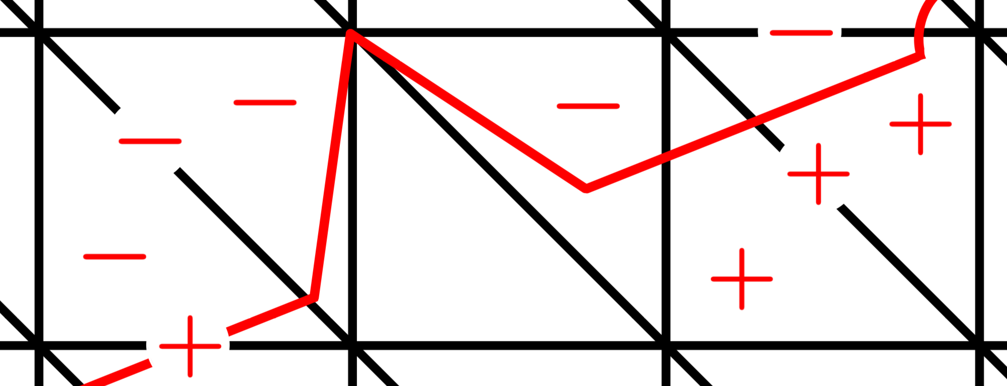
We denote the resulting generalized arc by $\widetilde{L_{t}}(w)_{-}$ . Construct the sequence associated to $\widetilde{L_{t}}(w)_{-}$ by applying the crossing rules and the endpoint rule in the same way as constructing $s(t)$ . Then the resulting sequence agrees with the sequence $w=(a_{k+1},a_{k+2},\dots,a_{k+n-1})$ corresponding to $\widetilde{L_{t}}(w)$ , except that its first (or last) entry is strictly smaller than $a_{k+1}$ (or $a_{k+n-1}$ ). We denote this sequence by

(b_{k+1},a_{k+2},\dots,a_{k+n-2},b_{k+n-1}),

where if $b_{k+1}=0$ , then $b_{k+1}$ is removed from the beginning of the sequence; the same convention applies to $b_{k+n-1}$ . In this situation,

m(\mathcal{G}[b_{k+1},a_{k+2},\dots,a_{k+n-2},b_{k+n-1}])<m(\mathcal{G}[w])

holds. Now $\widetilde{L_{t}}(a_{2},\dots,a_{n})$ corresponds to the line segment $L_{t}$ (defined in Section 2) with endpoints $A=(0,0)$ and $B=(q,p)$ ; this is precisely $\gamma_{AB}$ . Therefore, for any $w=(a_{k+1},a_{k+2},\dots,a_{k+n-2},a_{k+n-1})$ , if $\widetilde{L_{t}}(w)$ is a generalized arc, then $m(\mathcal{G}[w])$ coincides with the GM length of this arc, and hence

m(\mathcal{G}[a_{2},\dots,a_{n}])\leq m(\mathcal{G}[w]),

and if $\widetilde{L_{t}}(w)$ is not a generalized arc, then $m(\mathcal{G}[b_{k+1},a_{k+2},\dots,a_{k+n-2},b_{k+n-1}])$ coincides with the GM length of $\widetilde{L_{t}}(w)_{-}$ , and thus we have

m(\mathcal{G}[a_{2},\dots,a_{n}])\leq m(\mathcal{G}[b_{k+1},a_{k+2},\dots,a_{k+n-2},b_{k+n-1}])<m(\mathcal{G}[w])

by Theorem 5.7. Hence $m(\mathcal{G}[a_{2},\dots,a_{n}])$ attains the minimal value in $N_{t}$ , which completes the proof. ∎

This gives the following corollary, which identifies the corresponding Lagrange constant and Markov constant.

Corollary 6.3.

[s(t)^{\infty}]\in\mathbb{Q}[\sqrt{((3+k_{1}+k_{2}+k_{3})n_{t}-k_{t})^{2}-4}]

and

\mathcal{L}([s(t)^{\infty}])=\mathcal{M}(Q_{s(t)})=\frac{\sqrt{((3+k_{1}+k_{2}+k_{3})n_{t}-k_{t})^{2}-4}}{n_{t}}.

Proof.

We prove the former statement. Let $\alpha=[s(t)^{\infty}]$ . Then

\alpha=[s(t),\alpha].

By the general theory of continued-fraction matrices (see [8]*Appendix A), we have

\alpha=CF_{s(t)}(\alpha):=\dfrac{a\alpha+b}{c\alpha+d},

where $CF_{s(t)}=\begin{bmatrix}a&b\\ c&d\end{bmatrix}$ , and thus

c\alpha^{2}-(a-d)\alpha-b=0.

Therefore, we have

\alpha=\dfrac{a-d\pm\sqrt{(a-d)^{2}+4bc}}{2c}=\dfrac{a-d\pm\sqrt{(a+d)^{2}-4(ad-bc)}}{2c}.

Since $\alpha>0$ , we have

\alpha=\dfrac{a-d+\sqrt{(a+d)^{2}-4(ad-bc)}}{2c}.

When $t=\frac{0}{1}$ , the conclusion can be checked directly. We assume that $t\in(0,\infty].$ By Theorems 4.2 and 4.6, we have

\alpha=\dfrac{((3+k_{1}+k_{2}+k_{3})n_{t}-k_{t}-2u_{t}+\sqrt{((3+k_{1}+k_{2}+k_{3})n_{t}-k_{t})^{2}-4}}{2n_{t}}.

Therefore, we have

\alpha\in\mathbb{Q}[\sqrt{((3+k_{1}+k_{2}+k_{3})n_{t}-k_{t})^{2}-4}].

The asserted equality of the Lagrange constant and the Markov constant follows from Theorems 6.1, 2.20 and 2.22. ∎

Example 6.4.

Set $(k_{1},k_{2},k_{3},\sigma)=(1,2,0,\textrm{id})$ and $t=\tfrac{2}{5}$ . Then $i_{\frac{2}{5}}=1$ and

s\!\left(\tfrac{2}{5}\right)=(5,1,3,3,1,5,4,1,3,4).

Thus the sequences $w$ that contribute to $m(\mathcal{G}[w])\in N_{\frac{2}{5}}$ are

	$\displaystyle(1,3,3,1,5,4,1,3,4),\ (3,3,1,5,4,1,3,4,5),\ (3,1,5,4,1,3,4,5,1),\ (1,5,4,1,3,4,5,1,3),$
	$\displaystyle(5,4,1,3,4,5,1,3,3),\ (4,1,3,4,5,1,3,3,1),\ (1,3,4,5,1,3,3,1,5),\ (3,4,5,1,3,3,1,5,4),$
	$\displaystyle(4,5,1,3,3,1,5,4,1),\ (5,1,3,3,1,5,4,1,3).$

The corresponding values $m(\mathcal{G}[w])$ are

8227,\ 32957,\ 12039,\ 12041,\ 32937,\ 8261,\ 9997,\ 31881,\ 12199,\ 11127,

and the minimal number in $N_{\frac{2}{5}}$ is $8227$ . The corresponding arcs $\overline{L_{t}}(w)$ and $\widetilde{L_{t}}(w)$ are as in Table 2. Since

CF_{s(\frac{2}{5})}=\begin{bmatrix}m(\mathcal{G}[5,1,3,3,1,5,4,1,3,4])&m(\mathcal{G}[5,1,3,3,1,5,4,1,3])\\ m(\mathcal{G}[1,3,3,1,5,4,1,3,4])&m(\mathcal{G}[1,3,3,1,5,4,1,3])\end{bmatrix}=\begin{bmatrix}47431&11127\\ 8227&1930\end{bmatrix},

we have

[s(\tfrac{2}{5})^{\infty}]=\dfrac{\sqrt{2436508317}+45501}{16454},\quad L({}^{\infty}s(\tfrac{2}{5})^{\infty})=\dfrac{\sqrt{2436508317}}{8227}.

Moreover, we have

Q_{s(\frac{2}{5})}=x^{2}-\frac{45501}{8227}xy-\frac{11127}{8227}y^{2},

and thus

\mathcal{L}\left(\frac{\sqrt{2436508317}+45501}{16454}\right)=\mathcal{M}\left(x^{2}-\frac{45501}{8227}xy-\frac{11127}{8227}y^{2}\right)=\dfrac{\sqrt{2436508317}}{8227}.

[Uncaptioned image] — Table 2. $\overline{L_{t}}(w)$ and $\widetilde{L_{t}}(w)$

Remark 6.5.

Here are some tips for carrying out concrete example calculations:

(1)

For given $(k_{1},k_{2},k_{3})\in\mathbb{Z}_{\geq 0}^{3}$ and $\sigma\in\mathfrak{S}_{3}$ , the position $i_{t}$ corresponds to the edge of $\widetilde{\mathbb{R}^{2}}$ through which $L_{t}$ passes exactly at its midpoint. Namely, if this edge is horizontal, then $i_{t}=\sigma(1)$ ; if it is diagonal, then $i_{t}=\sigma(2)$ ; and if it is vertical, then $i_{t}=\sigma(3)$ . Moreover, $k_{t}$ coincides with the number of signs associated with this edge.
(2)

For an integer sequence $w=(b_{1},\dots,b_{n})$ , $m(\mathcal{G}[w])$ corresponds to the denominator of $[b_{1},\dots,b_{n}]$ and the numerator of $[b_{2},\dots,b_{n}]$ by Theorem 4.11.

6.2. Properties of Generalized Discrete Markov Spectra

Fix $(k_{1},k_{2},k_{3})\in\mathbb{Z}_{\geq 0}^{3}$ . For any $n\in\mathbb{Z}_{\geq 1}$ and $i\in\{1,2,3\}$ , we define

\Delta(n,i):=((3+k_{1}+k_{2}+k_{3})n-k_{i})^{2}-4.

We denote

\mathcal{M}_{k_{1},k_{2},k_{3},\sigma}:=\left\{\frac{\sqrt{\Delta(n_{t},i_{t})}}{n_{t}}\ \middle|\ \begin{aligned} (n_{t},i_{t})\text{ is a $(k_{1},k_{2},k_{3},\sigma)$-GM number-position pair}\end{aligned}\right\}

and consider

\mathcal{M}_{k_{1},k_{2},k_{3}}:=\bigcup_{\sigma\in\mathfrak{S}_{3}}\mathcal{M}_{k_{1},k_{2},k_{3},\sigma}.

We call the set $\mathcal{M}_{k_{1},k_{2},k_{3}}$ the $(k_{1},k_{2},k_{3})$ -generalized discrete Markov spectrum. For any $\sigma\in\mathfrak{S}_{3}$ , one has $\mathcal{M}_{k_{1},k_{2},k_{3}}=\mathcal{M}_{k_{\sigma(1)},k_{\sigma(2)},k_{\sigma(3)}}.$ Moreover, if $k_{1}=k_{2}=k_{3}=0$ , then $\mathcal{M}_{0,0,0}$ coincides with the ordinary discrete Markov spectrum $\mathcal{M}_{d}$ .

Corollary 6.3 immediately gives the following consequence.

Corollary 6.6.

For any $k_{1},k_{2},k_{3}\in\mathbb{Z}_{\geq 0}$ , $\mathcal{M}_{k_{1},k_{2},k_{3}}\subset\mathcal{L}$ and $\mathcal{M}_{k_{1},k_{2},k_{3}}\subset\mathcal{M}$ hold.

By the duality $(n_{t},i_{t})=(n^{\ast}_{\frac{1}{t}},i^{\ast}_{\frac{1}{t}})$ , even if $\sigma$ is restricted to the alternating group $\mathfrak{A}_{3}$ , the set $\mathcal{M}_{k_{1},k_{2},k_{3}}$ remains unchanged. Furthermore, even if we do not impose any restriction on $\sigma$ but instead restrict $t$ to the interval $[0,1]$ , the set $\mathcal{M}_{k_{1},k_{2},k_{3}}$ remains unchanged. Moreover, if two among $k_{1},k_{2},k_{3}$ are equal, then restricting $\sigma$ to $\mathfrak{A}_{3}$ and $t$ to $[0,1]$ does not alter $\mathcal{M}_{k_{1},k_{2},k_{3}}$ .

For any $(k_{1},k_{2},k_{3})\in\mathbb{Z}_{\geq 0}^{3}$ , the minimal $(k_{1},k_{2},k_{3})$ -GM number is $1$ . Therefore,

\mathcal{M}_{k_{1},k_{2},k_{3}}\subset[2+k_{i}+k_{j},3+k_{1}+k_{2}+k_{3}],

where $k_{i},k_{j}$ are the two smallest elements among $\{k_{1},k_{2},k_{3}\}$ .

Example 6.7.

We list some quadratic irrational numbers $\alpha$ and the corresponding Lagrange constants $\mathcal{L}(\alpha)$ obtained from Corollary 6.3. Table 3 shows the case $(k_{1},k_{2},k_{3})=(0,0,0)$ , Tables 4, 5, and 6 show the case $(k_{1},k_{2},k_{3})=(0,0,1)$ , Tables 7, 8, and 9 show the case $(k_{1},k_{2},k_{3})=(0,1,1)$ . Table 10 shows the case $(k_{1},k_{2},k_{3})=(1,1,1)$ , and Table 11 shows the case $(k_{1},k_{2},k_{3})=(2,2,2)$ . Table 12 shows the case $(k_{1},k_{2},k_{3},\sigma)=(1,2,0,\mathrm{id})$ . For each list, the elements are arranged in ascending order of the corresponding GM numbers.

$t$	$s(t)$	$\alpha=[s(t)^{\infty}]$	$n_{t}$	$\mathcal{L}(\alpha)$

$\dfrac{0}{1}$	$(1,1)$	$\dfrac{\sqrt{5}+1}{2}$	$1$	$\sqrt{5}$

$\dfrac{1}{1}$	$(2,2)$	${\sqrt{2}+1}$	$2$	$2\sqrt{2}$

$\dfrac{1}{2}$	$(2,1,1,2)$	$\dfrac{\sqrt{221}+11}{10}$	$5$	$\dfrac{\sqrt{221}}{5}$

$\dfrac{1}{3}$	$(2,1,1,1,1,2)$	$\dfrac{\sqrt{1517}+29}{26}$	$13$	$\dfrac{\sqrt{1517}}{13}$

$\dfrac{2}{3}$	$(2,1,1,2,2,2)$	$\dfrac{\sqrt{7565}+63}{58}$	$29$	$\dfrac{\sqrt{7565}}{29}$

$\dfrac{1}{4}$	$(2,1,1,1,1,1,1,2)$	$\dfrac{5\sqrt{26}+19}{17}$	$34$	$\dfrac{10\sqrt{26}}{17}$

$\dfrac{1}{5}$	$(2,1,1,1,1,1,1,1,1,2)$	$\dfrac{\sqrt{71285}+199}{178}$	$89$	$\dfrac{\sqrt{71285}}{89}$

$\dfrac{3}{4}$	$(2,1,1,2,2,2,2,2)$	$\dfrac{\sqrt{257045}+367}{338}$	$169$	$\dfrac{\sqrt{257045}}{169}$

Table 3. Case

(k_{1},k_{2},k_{3})=(0,0,0)

$t$	$s(t)$	$\alpha=[s(t)^{\infty}]$	$n_{t}$	$\mathcal{L}(\alpha)$

$\dfrac{0}{1}$	$(2,1)$	$\sqrt{3}+1$	$1$	$2\sqrt{3}$

$\dfrac{1}{1}$	$(3,2)$	$\dfrac{\sqrt{15}+3}{2}$	$2$	$\sqrt{15}$

$\dfrac{1}{2}$	$(3,1,1,3)$	$\dfrac{5\sqrt{29}+23}{14}$	$7$	$\dfrac{5\sqrt{29}}{7}$

$\dfrac{1}{3}$	$(3,1,2,1,1,3)$	$\dfrac{7\sqrt{51}+43}{25}$	$25$	$\dfrac{14\sqrt{51}}{25}$

$\dfrac{2}{3}$	$(3,1,1,3,3,2)$	$\dfrac{\sqrt{11235}+83}{53}$	$53$	$\dfrac{2\sqrt{11235}}{53}$

$\dfrac{1}{4}$	$(3,1,2,1,1,2,1,3)$	$\dfrac{\sqrt{15293}+107}{62}$	$93$	$\dfrac{\sqrt{15293}}{31}$

$\dfrac{1}{5}$	$(3,1,2,1,2,1,1,2,1,3)$	$\dfrac{3\sqrt{53207}+599}{346}$	$346$	$\dfrac{3\sqrt{53207}}{173}$

$\dfrac{3}{4}$	$(3,1,1,3,2,3,3,2)$	$\dfrac{\sqrt{308765}+435}{278}$	$417$	$\dfrac{2\sqrt{308765}}{278}$

Table 4. Case

(k_{1},k_{2},k_{3},\sigma)=(0,0,1,\mathrm{id})

$t$	$s(t)$	$\alpha=[s(t)^{\infty}]$	$n_{t}$	$\mathcal{L}(\alpha)$

$\dfrac{0}{1}$	$(2,1)$	$\sqrt{3}+1$	$1$	$2\sqrt{3}$

$\dfrac{1}{1}$	$(3,3)$	$\dfrac{\sqrt{13}+3}{2}$	3	$\sqrt{13}$

$\dfrac{1}{2}$	$(3,1,2,3)$	$\dfrac{\sqrt{399}+17}{10}$	$10$	$\dfrac{\sqrt{399}}{5}$

$\dfrac{1}{3}$	$(3,1,2,2,1,3)$	$\dfrac{\sqrt{21605}+127}{74}$	$37$	$\dfrac{\sqrt{21605}}{37}$

$\dfrac{2}{3}$	$(3,1,2,3,3,3)$	$\dfrac{\sqrt{47523}+185}{109}$	$109$	$\dfrac{2\sqrt{47523}}{109}$

$\dfrac{1}{4}$	$(3,1,2,1,2,2,1,3)$	$\dfrac{5\sqrt{3003}+237}{137}$	$137$	$\dfrac{10\sqrt{3003}}{137}$

$\dfrac{1}{5}$	$(3,1,2,1,2,2,1,2,1,3)$	$\dfrac{\sqrt{4173845}+1769}{1022}$	$511$	$\dfrac{\sqrt{4173845}}{511}$

$\dfrac{3}{4}$	$(3,1,2,3,3,3,3,3)$	$\dfrac{\sqrt{5654883}+2018}{1189}$	$1189$	$\dfrac{2\sqrt{5654883}}{1189}$

Table 5. Case

(k_{1},k_{2},k_{3},\sigma)=(0,0,1,(1\ 2\ 3))

$t$	$s(t)$	$\alpha=[s(t)^{\infty}]$	$n_{t}$	$\mathcal{L}(\alpha)$

$\dfrac{0}{1}$	$(1,1)$	$\dfrac{\sqrt{5}+1}{2}$	$1$	$\sqrt{5}$

$\dfrac{1}{1}$	$(3,2)$	$\dfrac{\sqrt{15}+3}{2}$	$2$	$\sqrt{15}$

$\dfrac{1}{2}$	$(3,1,1,2)$	$\dfrac{3\sqrt{11}+8}{5}$	$5$	$\dfrac{6\sqrt{11}}{5}$

$\dfrac{1}{3}$	$(3,1,1,1,1,2)$	$\dfrac{15\sqrt{3}+21}{13}$	$13$	$\dfrac{30\sqrt{3}}{13}$

$\dfrac{1}{4}$	$(3,1,1,1,1,1,1,2)$	$\dfrac{\sqrt{4623}+55}{34}$	$34$	$\dfrac{\sqrt{4623}}{17}$

$\dfrac{2}{3}$	$(3,1,1,3,2,2)$	$\dfrac{\sqrt{2669}+41}{26}$	$39$	$\dfrac{\sqrt{2669}}{13}$

$\dfrac{1}{5}$	$(3,1,1,1,1,1,1,1,1,2)$	$\dfrac{\sqrt{31683}+144}{89}$	$89$	$\dfrac{2\sqrt{31683}}{89}$

$\dfrac{1}{6}$	$(3,1,1,1,1,1,1,1,1,1,1,2)$	$\dfrac{\sqrt{217155}+377}{233}$	$233$	$\dfrac{2\sqrt{217155}}{233}$

Table 6. Case

(k_{1},k_{2},k_{3},\sigma)=(0,0,1,(1\ 3\ 2))

$t$	$s(t)$	$\alpha=[s(t)^{\infty}]$	$n_{t}$	$\mathcal{L}(\alpha)$

$\dfrac{0}{1}$	$(3,1)$	$\dfrac{\sqrt{21}+3}{2}$	$1$	$\sqrt{21}$

$\dfrac{1}{1}$	$(4,3)$	$\dfrac{4\sqrt{3}+6}{3}$	$3$	$\dfrac{8\sqrt{3}}{3}$

$\dfrac{1}{2}$	$(4,1,2,4)$	$\dfrac{\sqrt{1023}+29}{13}$	$13$	$\dfrac{2\sqrt{1023}}{13}$

$\dfrac{1}{3}$	$(4,1,3,2,1,4)$	$\dfrac{3\sqrt{2567}+139}{61}$	$61$	$\dfrac{6\sqrt{2567}}{61}$

$\dfrac{2}{3}$	$(4,1,2,4,4,3)$	$\dfrac{\sqrt{49506}+195}{89}$	$178$	$\dfrac{2\sqrt{49506}}{89}$

$\dfrac{1}{4}$	$(4,1,3,1,2,3,1,4)$	$\dfrac{44\sqrt{273}+666}{291}$	$291$	$\dfrac{88\sqrt{273}}{291}$

$\dfrac{1}{5}$	$(4,1,3,1,3,2,1,3,1,4)$	$\dfrac{531\sqrt{43}+3191}{1393}$	$1393$	$\dfrac{1062\sqrt{43}}{1393}$

$\dfrac{3}{4}$	$(4,1,2,4,3,4,4,3)$	$\dfrac{2\sqrt{9600702}+5431}{2479}$	$2479$	$\dfrac{4\sqrt{9600702}}{2479}$

Table 7. Case

(k_{1},k_{2},k_{3},\sigma)=(0,1,1,\mathrm{id})

$t$	$s(t)$	$\alpha=[s(t)^{\infty}]$	$n_{t}$	$\mathcal{L}(\alpha)$

$\dfrac{0}{1}$	$(2,1)$	$\sqrt{3}+1$	$1$	$2\sqrt{3}$

$\dfrac{1}{1}$	$(4,3)$	$\dfrac{4\sqrt{3}+6}{3}$	$3$	$\dfrac{8\sqrt{3}}{3}$

$\dfrac{1}{2}$	$(4,1,2,3)$	$\dfrac{2\sqrt{39}+11}{5}$	$10$	$\dfrac{4\sqrt{39}}{5}$

$\dfrac{1}{3}$	$(4,1,2,2,1,3)$	$\dfrac{\sqrt{8463}+82}{37}$	$37$	$\dfrac{2\sqrt{8463}}{37}$

$\dfrac{1}{4}$	$(4,1,2,1,2,2,1,3)$	$\dfrac{\sqrt{469221}+611}{274}$	$137$	$\dfrac{\sqrt{469221}}{137}$

$\dfrac{2}{3}$	$(4,1,2,4,3,3)$	$\dfrac{2\sqrt{30102}+305}{139}$	$139$	$\dfrac{4\sqrt{30102}}{139}$

$\dfrac{1}{5}$	$(4,1,2,1,2,2,1,2,1,3)$	$\dfrac{6\sqrt{45298}+1140}{511}$	$511$	$\dfrac{12\sqrt{45298}}{511}$

$\dfrac{2}{5}$	$(4,1,2,2,1,4,3,1,2,3)$	$\dfrac{22\sqrt{43662}+4050}{1839}$	$1839$	$\dfrac{44\sqrt{43662}}{1839}$

Table 8. Case

(k_{1},k_{2},k_{3},\sigma)=(0,1,1,(1\ 2\ 3))

$t$	$s(t)$	$\alpha=[s(t)^{\infty}]$	$n_{t}$	$\mathcal{L}(\alpha)$

$\dfrac{0}{1}$	$(2,1)$	$\sqrt{3}+1$	$1$	$2\sqrt{3}$

$\dfrac{1}{1}$	$(4,2)$	$\sqrt{6}+2$	$2$	$2\sqrt{6}$

$\dfrac{1}{2}$	$(4,1,1,3)$	$\dfrac{12\sqrt{2}+15}{7}$	$7$	$\dfrac{24\sqrt{2}}{7}$

$\dfrac{1}{3}$	$(4,1,2,1,1,3)$	$\dfrac{\sqrt{15621}+111}{50}$	$25$	$\dfrac{\sqrt{15621}}{25}$

$\dfrac{2}{3}$	$(4,1,1,4,3,2)$	$\dfrac{4\sqrt{1743}+138}{67}$	$67$	$\dfrac{8\sqrt{1743}}{67}$

$\dfrac{1}{4}$	$(4,1,2,1,1,2,1,3)$	$\dfrac{\sqrt{53823}+207}{93}$	$93$	$\dfrac{2\sqrt{53823}}{93}$

$\dfrac{1}{5}$	$(4,1,2,1,2,1,1,2,1,3)$	$\dfrac{12\sqrt{1299}+386}{173}$	$346$	$\dfrac{24\sqrt{1299}}{173}$

$\dfrac{3}{4}$	$(4,1,1,4,2,3,4,2)$	$\dfrac{\sqrt{2729103}+1356}{661}$	$661$	$\dfrac{2\sqrt{2729103}}{661}$

Table 9. Case

(k_{1},k_{2},k_{3},\sigma)=(0,1,1,(1\ 3\ 2))

$t$	$s(t)$	$\alpha=[s(t)^{\infty}]$	$n_{t}$	$\mathcal{L}(\alpha)$

$\dfrac{0}{1}$	$(3,1)$	$\dfrac{\sqrt{21}+3}{2}$	$1$	$\sqrt{21}$

$\dfrac{1}{1}$	$(5,3)$	$\dfrac{\sqrt{285}+15}{6}$	$3$	$\dfrac{\sqrt{285}}{3}$

$\dfrac{1}{2}$	$(5,1,2,4)$	$\dfrac{5\sqrt{237}+71}{26}$	$13$	$\dfrac{5\sqrt{237}}{13}$

$\dfrac{1}{3}$	$(5,1,3,2,1,4)$	$\dfrac{11\sqrt{1101}+339}{122}$	$61$	$\dfrac{11\sqrt{1101}}{61}$

$\dfrac{2}{3}$	$(5,1,2,5,4,3)$	$\dfrac{\sqrt{1692597}+1167}{434}$	$217$	$\dfrac{\sqrt{1692597}}{217}$

$\dfrac{1}{4}$	$(5,1,3,1,2,3,1,4)$	$\dfrac{\sqrt{3045021}+1623}{582}$	$291$	$\dfrac{\sqrt{3045021}}{291}$

$\dfrac{1}{5}$	$(5,1,3,1,3,2,1,3,1,4)$	$\dfrac{\sqrt{69839445}+7775}{2786}$	$1393$	$\dfrac{\sqrt{69839445}}{1393}$

$\dfrac{3}{4}$	$(5,1,2,5,3,4,5,3)$	$\dfrac{\sqrt{485629365}+19735}{7346}$	$3673$	$\dfrac{\sqrt{485629365}}{3673}$

Table 10. Case

(k_{1},k_{2},k_{3})=(1,1,1)

$t$	$s(t)$	$\alpha=[s(t)^{\infty}]$	$n_{t}$	$\mathcal{L}(\alpha)$

$\dfrac{0}{1}$	$(5,1)$	$\dfrac{3\sqrt{5}+5}{2}$	$1$	$3\sqrt{5}$

$\dfrac{1}{1}$	$(8,4)$	$3\sqrt{2}+4$	$4$	$6\sqrt{2}$

$\dfrac{1}{2}$	$(8,1,3,6)$	$\dfrac{3\sqrt{221}+43}{10}$	$25$	$\dfrac{3\sqrt{221}}{5}$

$\dfrac{1}{3}$	$(8,1,5,3,1,6)$	$\dfrac{3\sqrt{1517}+113}{26}$	$169$	$\dfrac{3\sqrt{1517}}{13}$

$\dfrac{2}{3}$	$(8,1,3,8,6,4)$	$\dfrac{3\sqrt{7565}+247}{58}$	$841$	$\dfrac{3\sqrt{7565}}{29}$

$\dfrac{1}{4}$	$(8,1,5,1,3,5,1,6)$	$\dfrac{15\sqrt{26}+74}{17}$	$1156$	$\dfrac{30\sqrt{26}}{17}$

$\dfrac{1}{5}$	$(8,1,5,1,5,3,1,5,1,6)$	$\dfrac{3\sqrt{71285}+775}{178}$	$7921$	$\dfrac{3\sqrt{71285}}{89}$

$\dfrac{3}{4}$	$(8,1,3,8,4,6,8,4)$	$\dfrac{3\sqrt{257045}+1439}{338}$	$28561$	$\dfrac{3\sqrt{257045}}{169}$

Table 11. Case

(k_{1},k_{2},k_{3})=(2,2,2)

$t$	$s(t)$	$\alpha=[s(t)^{\infty}]$	$n_{t}$	$\mathcal{L}(\alpha)$

$\dfrac{0}{1}$	$(3,1)$	$\dfrac{\sqrt{2}1+3}{2}$	$1$	$\sqrt{21}$

$\dfrac{1}{1}$	$(5,4)$	$\dfrac{{\sqrt{30}+5}}{2}$	$4$	$\sqrt{30}$

$\dfrac{1}{2}$	$(5,1,3,4)$	$\dfrac{10\sqrt{26}+47}{17}$	$17$	$\dfrac{20\sqrt{26}}{17}$

$\dfrac{1}{3}$	$(5,1,3,3,1,4)$	$\dfrac{\sqrt{723}+25}{9}$	$81$	$\dfrac{2\sqrt{723}}{9}$

$\dfrac{2}{3}$	$(5,1,3,5,4,4)$	$\dfrac{\sqrt{5004165}+2061}{746}$	$373$	$\dfrac{\sqrt{5004165}}{373}$

$\dfrac{1}{4}$	$(5,1,3,1,3,3,1,4)$	$\dfrac{\sqrt{1340963}+1077}{386}$	$386$	$\dfrac{\sqrt{1340963}}{193}$

$\dfrac{1}{5}$	$(5,1,3,1,3,3,1,3,1,4)$	$\dfrac{\sqrt{16635}+120}{43}$	$1849$	$\dfrac{2\sqrt{16635}}{43}$

$\dfrac{3}{4}$	$(5,1,3,5,4,4,5,4)$	$\dfrac{2\sqrt{150737006}+22602}{8185}$	$8185$	$\dfrac{4\sqrt{150737006}}{8185}$

Table 12. Case

(k_{1},k_{2},k_{3},\sigma)=(1,2,0,\mathrm{id})

We now describe a special relation between $\mathcal{M}_{0,0,0}$ and $\mathcal{M}_{2,2,2}$ . The following relation is known.

Proposition 6.8 ([21]*Theorem 11).

If $(a,b,c)$ is a $(0,0,0)$ -GM triple, then $(a^{2},b^{2},c^{2})$ is a $(2,2,2)$ -GM triple. Conversely, if $(A,B,C)$ is a $(2,2,2)$ -GM triple, then $(\sqrt{A},\sqrt{B},\sqrt{C})$ is a $(0,0,0)$ -GM triple.

Proposition 6.8 gives the following relation between the two spectra.

Theorem 6.9.

If $r\in\mathcal{M}_{0,0,0}$ , then $3r\in\mathcal{M}_{2,2,2}$ . Conversely, if $R\in\mathcal{M}_{2,2,2}$ , then $\frac{R}{3}\in\mathcal{M}_{0,0,0}$ .

Proof.

We first prove the forward implication. Since $r\in\mathcal{M}_{0,0,0}$ , there exists a $(0,0,0)$ -GM number $n$ such that

r=\frac{\sqrt{9n^{2}-4}}{n}.

Thus

3r=\frac{3\sqrt{9n^{2}-4}}{n}=\frac{\sqrt{81n^{4}-36n^{2}}}{n^{2}}=\frac{\sqrt{(9n^{2}-2)^{2}-4}}{n^{2}}.

By Proposition 6.8, $n^{2}$ is a $(2,2,2)$ -GM number, and hence $3r\in\mathcal{M}_{2,2,2}$ . The reverse implication follows by reversing the above computation. ∎

We next characterize generalized discrete Markov spectra in the transition interval.

Theorem 6.10.

Set

\mathcal{M}^{\prime}=\bigcup_{(k_{1},k_{2},k_{3})\in\mathbb{Z}_{\geq 0}^{3}}\mathcal{M}_{k_{1},k_{2},k_{3}}.

Then we have

\mathcal{M}^{\prime}\cap[3,c_{F})=(\mathcal{M}_{0,0,1}\setminus\{\sqrt{5}\})\cup\{2\sqrt{5}\},

where $c_{F}$ is the Freiman constant, i.e.,

c_{F}:=\dfrac{2221564096+283748\sqrt{462}}{491993569}\approx 4.5278295661\dots.

Proof.

Without loss of generality, assume $k_{1}\leq k_{2}\leq k_{3}$ . We first prove $\mathcal{M}^{\prime}\cap[3,c_{F})\supset(\mathcal{M}_{0,0,1}\setminus\{\sqrt{5}\})\cup\{2\sqrt{5}\}$ . The inclusion $\mathcal{M}_{0,0,1}\setminus\{\sqrt{5}\}\subset\mathcal{M}^{\prime}$ is immediate. Moreover, we have $2\sqrt{5}\in\mathcal{M}_{0,0,2}\subset\mathcal{M}^{\prime}$ . Indeed, $(4,3)$ is a $(0,0,2,\mathrm{(1\ 2\ 3)})$ -GM number-position pair, and the corresponding element of $\mathcal{M}_{0,0,2}$ is

\frac{\sqrt{(5\cdot 4-2)^{2}-4}}{4}=\frac{\sqrt{320}}{4}=2\sqrt{5}.

We prove $(\mathcal{M}_{0,0,1}\setminus\{\sqrt{5}\})\cup\{2\sqrt{5}\}\subset[3,c_{F})$ . The element $2\sqrt{5}$ lies in $[3,c_{F})$ . The functions

f(x)=\frac{\sqrt{(4x)^{2}-4}}{x},\quad g(x)=\frac{\sqrt{(4x-1)^{2}-4}}{x}

are both increasing monotonically on $x\geq 1$ , and

\lim_{x\to\infty}f(x)=\lim_{x\to\infty}g(x)=4.

Therefore, we have $\mathcal{M}_{0,0,1}\subset[0,c_{F}]$ . The minimal element of $\mathcal{M}_{0,0,1}\setminus\{\sqrt{5}\}$ is $2\sqrt{3}$ by Tables 4, 5, 6, therefore we have $\mathcal{M}_{0,0,1}\setminus\{\sqrt{5}\}\subset[3,c_{F})$ .

We next prove $\mathcal{M}^{\prime}\cap[3,c_{F})\subset(\mathcal{M}_{0,0,1}\setminus\{\sqrt{5}\})\cup\{2\sqrt{5}\}$ . It is enough to observe that

\mathcal{M}_{0,0,0}\cap[3,c_{F})=\emptyset,\text{ and }\mathcal{M}_{0,0,1}\cap[3,c_{F})=\mathcal{M}_{0,0,1}\setminus\{\sqrt{5}\}.

We assume $k_{1}=k_{2}=0$ and $k_{3}=k\in\mathbb{Z}_{\geq 2}$ . We determine the order of the small elements of $\mathcal{M}_{0,0,k}$ . In this case, all $(0,0,k)$ -GM number-position pairs are in

\left\{(n_{t},i_{t})\in v\ \middle|\ v\in\bigcup_{\sigma\in\mathfrak{A}_{3}}\mathrm{M}\mathbb{T}(0,0,k,\sigma),t\in[0,1]\right\}.

First, we assume that $k_{t}=0$ for $t\in[0,1]$ . Then the minimum element and the second minimum element are as follows:

$\sigma$	Minimum $n_{t}$	Second minimum $n_{t}$

$\mathrm{id}$	$n_{\frac{0}{1}}=1$	$n_{\frac{1}{1}}=2$

$(1\ 2\ 3)$	$n_{\frac{0}{1}}=1$	$n_{\frac{1}{2}}=k^{2}+4k+5$

$(1\ 3\ 2)$	$n_{\frac{1}{1}}=2$	$n_{\frac{1}{2}}=5$

Hence, in this range, the $(0,0,k)$ -GM numbers are arranged in ascending order as $1,2,5$ . The corresponding elements of $\mathcal{M}_{0,0,k}$ to $n=1,2,5$ are

\sqrt{k^{2}+6k+5},\sqrt{k^{2}+6k+8},\sqrt{k^{2}+6k+\dfrac{221}{25}}

Next, we assume that $k_{t}=k$ for $t\in[0,1]$ . Then the minimum element and the second minimum element are as follows:

$\sigma$	Minimum $n_{t}$	Second minimum $n_{t}$

$\mathrm{id}$	$n_{\frac{1}{2}}=2k+5$	$n_{\frac{1}{4}}=2k^{3}+16k^{2}+41k+34$

$(1\ 2\ 3)$	$n_{\frac{1}{1}}=k+2$	$n_{\frac{1}{3}}=2k^{2}+10k+13$

$(1\ 3\ 2)$	$n_{\frac{0}{1}}=1$	$n_{\frac{2}{3}}=10k+29$

Hence, in this range, the $(0,0,k)$ -GM numbers are arranged in ascending order as $1,k+2,2k+5$ . The corresponding elements of $\mathcal{M}_{0,0,k}$ to $n=1,k+2,2k+5$ are

\sqrt{5},\sqrt{k^{2}+4k+8},\sqrt{k^{2}+5k+\dfrac{35}{4}+\dfrac{9}{4(2k+5)^{2}}}.

Therefore, first two minimum elements of $\mathcal{M}_{0,0,k}$ are

\sqrt{5},\sqrt{k^{2}+4k+8}.

if $k\geq 2$ . The third minimum element is

\begin{cases}\sqrt{k^{2}+6k+5}\quad&\text{if }k=2,3,\vskip 8.53581pt\\ \sqrt{k^{2}+5k+\dfrac{35}{4}+\dfrac{9}{4(2k+5)^{2}}}\quad&\text{otherwise.}\end{cases}

Among these values, the only one lying in $[3,c_{F})$ is $\sqrt{k^{2}+4k+8}=2\sqrt{5}$ , which occurs when $k=2$ . Therefore, we have

\mathcal{M}_{0,0,2}\cap[3,c_{F})=\{2\sqrt{5}\},

and for any $k\geq 3$ ,

\mathcal{M}_{0,0,k}\cap[3,c_{F})=\emptyset.

Next, we assume that $k_{1}=0$ and $k_{2}=k_{3}=1$ . By Tables 7, 8, 9, we have

\mathcal{M}_{0,1,1}\cap[3,c_{F})=\{2\sqrt{3}\},

and $2\sqrt{3}\in\mathcal{M}_{0,0,1}$ .

Let us prove the remaining cases. We set $K:=3+k_{1}+k_{2}+k_{3}$ . The remaining cases all satisfy $K\geq 6$ and the condition that $k_{i}\leq K-4$ for every $i$ . Hence, from now on we shall assume these conditions. If the following inequality holds

\dfrac{\sqrt{(Kn_{t}-k_{t})^{2}-4}}{n_{t}}<5,

then by assumption we have

\dfrac{\sqrt{(Kn_{t}-K+4)^{2}-4}}{n_{t}}\leq\dfrac{\sqrt{(Kn_{t}-k_{t})^{2}-4}}{n_{t}}<5.

From the two sides of this inequality we obtain the following inequality:

(K^{2}-25)n_{t}^{2}+(-2K^{2}+8K)n_{t}+(K^{2}-8K+12)<0.

Since $K\geq 6$ , we have $K^{2}-25>0$ and thus

\dfrac{K(K-4)-\sqrt{29K^{2}-200K+300}}{K^{2}-25}<n_{t}<\dfrac{K(K-4)+\sqrt{29K^{2}-200K+300}}{K^{2}-25}.

Now, the function $F(x)=\dfrac{x(x-4)+\sqrt{29x^{2}-200x+300}}{x^{2}-25}$ is monotonically decreasing on $x\geq 6$ , as one checks from $F^{\prime}(x)<0$ . Therefore, we have

n_{t}<\dfrac{6(6-4)+\sqrt{29\cdot 36-200\cdot 6+300}}{36-25}=\frac{8}{3}.

Therefore, if

\dfrac{\sqrt{((3+k_{1}+k_{2}+k_{3})n_{t}-k_{t})^{2}-4}}{n_{t}}\in[3,c_{F}),

then $n_{t}$ must be $1$ or $2$ . First, we assume $n_{t}=1$ . If $\sqrt{(3+k_{1}+k_{2}+k_{3}-k_{t})^{2}-4}\in[3,c_{F})$ , then $k_{1}+k_{2}+k_{3}-k_{t}=1$ . We have thus $k_{1}=0$ , $k_{2}=1$ , $k_{t}=k_{3}$ and

\sqrt{(3+k_{1}+k_{2}+k_{3}-k_{t})^{2}-4}=2\sqrt{3}\in\mathcal{M}_{0,0,1}.

Second, we assume that $n_{t}=2$ . Now, $k_{t}$ must be $0$ and thus $k_{1}=0$ . Then we have

\dfrac{\sqrt{((3+k_{1}+k_{2}+k_{3})n_{t}-k_{i})^{2}-4}}{n_{t}}=\dfrac{\sqrt{(2\cdot(3+k_{2}+k_{3}))^{2}-4}}{2}

From the assumption, $k_{2}+k_{3}$ must be at least $3$ , but then

\dfrac{\sqrt{(2\cdot(3+k_{2}+k_{3}))^{2}-4}}{2}\notin[3,c_{F}).

The preceding argument shows that, if $k\geq 2$ , then

\mathcal{M}_{0,1,k}\cap[3,c_{F})=\{2\sqrt{3}\}\subset\mathcal{M}_{0,0,1},

and if $(k_{1},k_{2},k_{3})$ does not have the form $(0,0,0),(0,0,k)$ or $(0,1,k)$ , then we have

\mathcal{M}_{k_{1},k_{2},k_{3}}\cap[3,c_{F})=\emptyset.

This finishes the proof. ∎

Remark 6.11.

The set $\mathcal{M}^{\prime}\cap[3,c_{F})$ does not cover all Lagrange constants contained in the transition interval. In other words, the strict inclusion

\mathcal{M}^{\prime}\cap[3,c_{F})\subsetneq\mathcal{L}\cap[3,c_{F})

holds. To prove this, set $s=(1,1,1,2,2,2)$ , and

\alpha=[(1,1,1,2,2,2)^{\infty}]=\frac{2\sqrt{210}+17}{29}.

Using Theorem 2.20 and Lemma 6.2, we have

\mathcal{L}(\alpha)=\frac{4\sqrt{210}}{19}\approx 3.05081615709...,

and $\mathcal{L}(\alpha)\in\mathcal{L}\cap[3,c_{F})$ . On the other hand, the minimal element of $\mathcal{M}^{\prime}\cap[3,c_{F})$ is

2\sqrt{3}\approx 3.46410161514\dots,

and $\mathcal{L}(\alpha)\notin\mathcal{M}^{\prime}\cap[3,c_{F})$ .

Theorem 2.25 states that the discrete Markov spectrum coincides with the part of the Markov spectrum below $3$ . A corresponding theorem for GM numbers is not yet known.

Question 6.12.

Is there a characterization of $\mathcal{M}_{k_{1},k_{2},k_{3}}$ , or of their union, that generalizes Markov’s theorem?

6.3. Boundary Values from Irrational Slopes

In this subsection, we keep $(k_{1},k_{2},k_{3})\in\mathbb{Z}_{\geq 0}^{3}$ and $\sigma\in\mathfrak{S}_{3}$ fixed, and put

K:=3+k_{1}+k_{2}+k_{3}.

We consider only positive slopes, in accordance with the definition of the generalized strongly admissible sequence $s(t)$ for $t\in[0,\infty]\cap\mathbb{Q}$ . A line of positive slope is oriented in the direction in which the $x$ -coordinate increases. Reversing this orientation only reverses the resulting integer sequence and hence does not change the two-sided continued-fraction quantity defined below.

Let $\mathcal{P}$ denote the set consisting of all lattice points and all midpoints of edges in $\widetilde{\mathbb{R}^{2}}$ . We call a line regular if it does not pass through any point of $\mathcal{P}$ .

Definition 6.13.

Let $l$ be an oriented regular line of positive irrational slope. Apply the triangle-crossing and edge-crossing rules to $l$ , and arrange the resulting signs in the order in which $l$ passes through them. By recording the lengths of consecutive runs of equal signs, we obtain a two-sided infinite sequence of positive integers, denoted by

\mathbf{b}(l)=(b_{n})_{n\in\mathbb{Z}}.

The origin of the index is chosen arbitrarily, so $\mathbf{b}(l)$ is determined only up to shift.

We use the functions $\ell_{r}(\mathbf{a})$ and $L(\mathbf{a})$ for bi-infinite positive integer sequences as defined in Section 2. Since $L(\mathbf{a})$ is invariant under shifts, the arbitrary choice of the index origin in the definition of $\mathbf{b}(l)$ is harmless.

The goal of this subsection is the following theorem.

Theorem 6.14.

Let $(k_{1},k_{2},k_{3})\in\mathbb{Z}_{\geq 0}^{3}$ and $\sigma\in\mathfrak{S}_{3}$ be fixed, and put $K=3+k_{1}+k_{2}+k_{3}$ . If $l$ is a regular line of positive irrational slope in $\widetilde{\mathbb{R}^{2}}$ , then

L(\mathbf{b}(l))=K.

We prepare several elementary lemmas.

Lemma 6.15.

For every $\varepsilon>0$ , there exists $N\geq 1$ such that, if two bi-infinite positive integer sequences $\mathbf{a}=(a_{n})_{n\in\mathbb{Z}}$ and $\mathbf{c}=(c_{n})_{n\in\mathbb{Z}}$ satisfy

a_{i}=c_{i}\qquad(-N\leq i\leq N),

then

|\ell_{0}(\mathbf{a})-\ell_{0}(\mathbf{c})|<\varepsilon.

Proof.

The value $\ell_{0}(\mathbf{a})$ is defined as

[a_{0};a_{1},a_{2},\ldots]+[0;a_{-1},a_{-2},\ldots].

For the right infinite continued fraction $[a_{0};a_{1},a_{2},\ldots]$ , all values whose first $N+1$ partial quotients coincide lie in the same continued-fraction cylinder. If $q_{N}$ denotes the corresponding denominator, then the length of this cylinder is at most $1/(q_{N}(q_{N}+q_{N-1}))$ . Since all partial quotients are at least $1$ , the denominator $q_{N}$ is bounded from below by the denominator obtained when the first $N+1$ partial quotients are all $1$ . Hence this cylinder length is bounded above by a quantity independent of the sequence and tending to $0$ as $N\to\infty$ . The same argument applies to the left infinite continued fraction $[0;a_{-1},a_{-2},\ldots]$ . Taking $N$ sufficiently large makes the sum of the two errors smaller than $\varepsilon$ . ∎

Lemma 6.16.

Let $l$ be a regular line of positive irrational slope. Then every finite block appearing in $\mathbf{b}(l)$ also appears in the periodic sequence

{}^{\infty}s(t)^{\infty}=(\ldots,s(t),s(t),s(t),\ldots)

for some irreducible fraction $t\in(0,\infty)\cap\mathbb{Q}$ with sufficiently large denominator.

Proof.

Fix a finite block of $\mathbf{b}(l)$ . This block is determined by a finite segment of $l$ , namely by the order in which that segment crosses triangles and edges of $\widetilde{\mathbb{R}^{2}}$ and by the signs assigned to them. Since $l$ is regular, this finite segment has positive distance from the finite set of relevant exceptional points in $\mathcal{P}$ . Thus the crossing order and the assigned signs in this finite region are unchanged if the slope and intercept of the line are changed sufficiently slightly.

Write the slope and intercept of $l$ as $\tau$ and $\theta$ , respectively. Choose an irreducible rational number $t=p/q$ sufficiently close to $\tau$ . If $q$ is sufficiently large, then integer translates of the line of slope $t$ used to define $s(t)$ have intercepts that approximate $\theta$ arbitrarily well: translating by an integer vector $(m,n)$ changes the intercept by $n-tm$ , and, since $t=p/q$ with $(p,q)=1$ , these values run through a translate of $q^{-1}\mathbb{Z}$ . Hence one can choose an integer translate whose intercept is sufficiently close to $\theta$ .

For this translated rational-slope line, the fixed finite region yields the same sign pattern, and hence the same integer block. Integer translations preserve the triangle-crossing and edge-crossing rules, so the two-sided sequence obtained from this line is a shift of ${}^{\infty}s(t)^{\infty}$ . Therefore the fixed finite block also appears in ${}^{\infty}s(t)^{\infty}$ . ∎

Lemma 6.17.

Let $l$ and $l^{\prime}$ be regular lines with the same positive irrational slope. Then the set of finite blocks appearing in $\mathbf{b}(l)$ coincides with the set of finite blocks appearing in $\mathbf{b}(l^{\prime})$ .

Proof.

Let the common slope be $\tau\notin\mathbb{Q}$ . Translating $l$ by an integer vector $(m,n)$ changes its intercept by $n-\tau m$ . By the density of irrational rotations, these changes are dense modulo $1$ .

Fix a finite block appearing in $\mathbf{b}(l)$ . Because $l$ is regular, the finite segment producing this block is stable under sufficiently small parallel translations. By the density above, some integer translate of $l$ can be made sufficiently close to $l^{\prime}$ in the relevant finite region. The translated segment then gives the same sign pattern and hence the same integer block. Since integer translations preserve the sign rules, this block appears in $\mathbf{b}(l^{\prime})$ . The reverse inclusion is proved in the same way. ∎

Lemma 6.18.

For every positive irreducible fraction $t\in(0,\infty)\cap\mathbb{Q}$ , one has

L({}^{\infty}s(t)^{\infty})<K.

Moreover, if $(t_{j})_{j\geq 0}$ is a sequence of distinct positive irreducible fractions converging to an irrational number $\tau$ , then

\lim_{j\to\infty}L({}^{\infty}s(t_{j})^{\infty})=K.

Proof.

By Theorem 6.1, if $(n_{t},i_{t})$ is the $(k_{1},k_{2},k_{3},\sigma)$ -GM number-position pair corresponding to $t$ , then

L({}^{\infty}s(t)^{\infty})=\frac{\sqrt{(Kn_{t}-k_{t})^{2}-4}}{n_{t}}.

The right-hand side is strictly smaller than $K$ .

Now suppose that $t_{j}\to\tau\notin\mathbb{Q}$ and that the $t_{j}$ are distinct. Writing $t_{j}=p_{j}/q_{j}$ in lowest terms, we have $p_{j}+q_{j}\to\infty$ . Hence the number of triangles and edges crossed by $L_{t_{j}}$ tends to infinity, so the length of the generalized strongly admissible sequence $s(t_{j})$ tends to infinity. By Theorem 4.6, $n_{t_{j}}$ is the $(2,1)$ -entry of $CF_{s(t_{j})}$ . Since the entries of $s(t_{j})$ are positive and its length tends to infinity, we have $n_{t_{j}}\to\infty$ . As $k_{t_{j}}$ belongs to the fixed finite set $\{k_{1},k_{2},k_{3}\}$ , it follows that

\frac{\sqrt{(Kn_{t_{j}}-k_{t_{j}})^{2}-4}}{n_{t_{j}}}=\sqrt{\left(K-\frac{k_{t_{j}}}{n_{t_{j}}}\right)^{2}-\frac{4}{n_{t_{j}}^{2}}}\longrightarrow K.

∎

Proof of Theorem 6.14.

We first prove $L(\mathbf{b}(l))\leq K$ . Fix $r\in\mathbb{Z}$ . It suffices to prove $\ell_{r}(\mathbf{b}(l))\leq K$ .

Let $\varepsilon>0$ . By Lemma 6.15, if $N$ is sufficiently large, then the value of $\ell_{r}$ is determined up to an error less than $\varepsilon$ by the central finite block

b_{r-N},\ldots,b_{r},\ldots,b_{r+N}.

By Lemma 6.16, this finite block also appears in ${}^{\infty}s(t)^{\infty}$ for some rational slope $t$ . Hence, for some position $j$ ,

\ell_{r}(\mathbf{b}(l))\leq\ell_{j}({}^{\infty}s(t)^{\infty})+\varepsilon.

By Lemma 6.18, we obtain

\ell_{r}(\mathbf{b}(l))\leq L({}^{\infty}s(t)^{\infty})+\varepsilon<K+\varepsilon.

Since $\varepsilon>0$ was arbitrary, $\ell_{r}(\mathbf{b}(l))\leq K$ . Since $r$ was arbitrary, $L(\mathbf{b}(l))\leq K$ .

We next prove $L(\mathbf{b}(l))\geq K$ . Let $\tau$ be the slope of $l$ , and choose a sequence of distinct positive irreducible fractions $t_{j}\in(0,\infty)\cap\mathbb{Q}$ converging to $\tau$ . By Lemma 6.18,

L({}^{\infty}s(t_{j})^{\infty})\longrightarrow K.

For each $j$ , choose a position in the periodic sequence ${}^{\infty}s(t_{j})^{\infty}$ at which the value $L({}^{\infty}s(t_{j})^{\infty})$ is attained, and shift the sequence so that this position becomes $0$ . Denote the shifted sequence by $\mathbf{c}^{(j)}$ . Thus

\ell_{0}(\mathbf{c}^{(j)})=L({}^{\infty}s(t_{j})^{\infty}).

We first observe that the entries of all $\mathbf{c}^{(j)}$ are uniformly bounded. For every $n\in\mathbb{Z}$ ,

c^{(j)}_{n}<\ell_{n}(\mathbf{c}^{(j)})\leq L(\mathbf{c}^{(j)})<K.

Since $K$ is an integer and $c^{(j)}_{n}$ is a positive integer, we have

c^{(j)}_{n}\in\{1,2,\ldots,K-1\}

for all $j$ and $n$ .

Order the integers as $0,1,-1,2,-2,\ldots$ . By repeatedly passing to subsequences and then taking the diagonal subsequence, we may assume that, for every fixed $n\in\mathbb{Z}$ , the value $c^{(j)}_{n}$ is eventually constant. Define

c_{n}:=\lim_{j\to\infty}c^{(j)}_{n},\qquad\mathbf{c}=(c_{n})_{n\in\mathbb{Z}}.

We claim that $\ell_{0}(\mathbf{c}^{(j)})\to\ell_{0}(\mathbf{c})$ . Indeed, given $\varepsilon>0$ , choose $N$ by Lemma 6.15. For all sufficiently large $j$ , the two sequences $\mathbf{c}^{(j)}$ and $\mathbf{c}$ agree on $[-N,N]$ , and hence $|\ell_{0}(\mathbf{c}^{(j)})-\ell_{0}(\mathbf{c})|<\varepsilon$ . Therefore $\ell_{0}(\mathbf{c}^{(j)})\to\ell_{0}(\mathbf{c})$ . Since the left-hand side also tends to $K$ , we get

\ell_{0}(\mathbf{c})=K.

We now show that every finite block of $\mathbf{c}$ also appears in $\mathbf{b}(l)$ . Fix a central block

W=(c_{-N},c_{-N+1},\ldots,c_{N}).

By construction of the diagonal subsequence, for all sufficiently large $j$ this block appears as

(c^{(j)}_{-N},c^{(j)}_{-N+1},\ldots,c^{(j)}_{N})=W.

The sequence $\mathbf{c}^{(j)}$ is a shift of the periodic sequence obtained from a rational-slope line of slope $t_{j}$ , and $t_{j}\to\tau$ . Let $\gamma_{j}$ be a finite line segment of slope $t_{j}$ that reads the block $W$ . Since the triangular decomposition and the sign rules are periodic under integer translations, we may translate $\gamma_{j}$ by an integer vector without changing the block it reads. We do this so that the midpoint of $\gamma_{j}$ lies in the fundamental square $[0,1]^{2}$ .

By compactness of $[0,1]^{2}$ , after passing to a subsequence we may assume that these midpoints converge to some point $P\in[0,1]^{2}$ . Since the slopes satisfy $t_{j}\to\tau$ , the finite line segments $\gamma_{j}$ converge to a finite line segment $\gamma$ of slope $\tau$ passing through $P$ .

If $\gamma$ does not pass through any point of $\mathcal{P}$ , then the sign rules are locally constant near $\gamma$ , and hence $\gamma$ reads the same finite block $W$ . Suppose instead that $\gamma$ passes through a point of $\mathcal{P}$ . Since $\tau$ is irrational, a line of slope $\tau$ can pass through at most one point of $\mathcal{P}$ : if it passed through two such points, the coordinate difference of these two points would lie in $(\frac{1}{2}\mathbb{Z})^{2}$ , forcing the slope to be rational. Passing to a further subsequence if necessary, we may assume that the segments $\gamma_{j}$ pass on the same side of this exceptional point. Keeping the slope $\tau$ fixed, translate $\gamma$ by a sufficiently small amount toward that side. This removes the singularity in the same way as for the approximating segments, so the translated segment still reads the block $W$ . The translation can also be chosen to avoid the countable set of intercepts for which a point of $\mathcal{P}$ lies on the line. Thus $W$ is realized by a regular line of slope $\tau$ .

By Lemma 6.17, the set of finite blocks produced by regular lines of slope $\tau$ is independent of the intercept. Hence every finite block of $\mathbf{c}$ appears in the original sequence $\mathbf{b}(l)$ .

Finally let $\varepsilon>0$ . Choose $N$ by Lemma 6.15. The central block $W$ appears in $\mathbf{b}(l)$ , so for some position $q$ we have

\ell_{q}(\mathbf{b}(l))>\ell_{0}(\mathbf{c})-\varepsilon=K-\varepsilon.

Therefore $L(\mathbf{b}(l))\geq K-\varepsilon$ . Since $\varepsilon>0$ was arbitrary, $L(\mathbf{b}(l))\geq K$ . Combining the two inequalities gives $L(\mathbf{b}(l))=K$ . ∎

Remark 6.19.

For $(k_{1},k_{2},k_{3})=(0,0,0)$ , this theorem corresponds to the fact that the two-sided sequences obtained by substituting $X\mapsto(2,2)$ and $Y\mapsto(1,1)$ into mechanical words of irrational slope have the boundary value $3$ . Thus Theorem 6.14 can be viewed as a sign-rule formulation of the fact that the discrete constants produced by generalized strongly admissible sequences of rational slope accumulate at $3+k_{1}+k_{2}+k_{3}$ .

We now show that the same boundary value is realized as a Lagrange constant.

Corollary 6.20.

Let $(k_{1},k_{2},k_{3})\in\mathbb{Z}_{\geq 0}^{3}$ and $\sigma\in\mathfrak{S}_{3}$ be fixed, and put $K=3+k_{1}+k_{2}+k_{3}$ . Let $l$ be a regular line of positive irrational slope, and let

\mathbf{b}(l)=(b_{n})_{n\in\mathbb{Z}}

be the bi-infinite sequence of positive integers obtained from $l$ by the triangle-crossing and edge-crossing rules. For any $r\in\mathbb{Z}$ , put

\alpha_{r}:=[b_{r};b_{r+1},b_{r+2},\ldots].

Then

\mathcal{L}(\alpha_{r})=K.

In particular, $K\in\mathcal{L}$ .

Proof.

It is enough to prove the case $r=0$ , since the other cases are obtained by shifting the indices of $\mathbf{b}(l)$ . Put

\alpha:=[b_{0};b_{1},b_{2},\ldots].

By the Perron identity (Theorem 2.20), we have

\mathcal{L}(\alpha)=\limsup_{n\to\infty}\left([b_{n+1};b_{n+2},b_{n+3},\ldots]+[0;b_{n},b_{n-1},\ldots,b_{1}]\right).

On the other hand, for the bi-infinite sequence $\mathbf{b}(l)$ we have

\ell_{n+1}(\mathbf{b}(l))=[b_{n+1};b_{n+2},b_{n+3},\ldots]+[0;b_{n},b_{n-1},\ldots].

The two continued fractions

[0;b_{n},b_{n-1},\ldots,b_{1}]\quad\text{and}\quad[0;b_{n},b_{n-1},\ldots]

have the same first $n$ partial quotients. Hence the usual cylinder estimate for regular continued fractions gives

\left|[0;b_{n},b_{n-1},\ldots,b_{1}]-[0;b_{n},b_{n-1},\ldots]\right|\longrightarrow 0\qquad(n\to\infty).

Therefore

\mathcal{L}(\alpha)=\limsup_{n\to\infty}\ell_{n+1}(\mathbf{b}(l)).

By Theorem 6.14, $L(\mathbf{b}(l))=K$ . Hence $\ell_{n}(\mathbf{b}(l))\leq K$ for all $n\in\mathbb{Z}$ , and so

\mathcal{L}(\alpha)=\limsup_{n\to\infty}\ell_{n+1}(\mathbf{b}(l))\leq K.

We prove the reverse inequality. Let $\varepsilon>0$ . Since $L(\mathbf{b}(l))=K$ , there exists $r_{0}\in\mathbb{Z}$ such that

\ell_{r_{0}}(\mathbf{b}(l))>K-\varepsilon.

By Lemma 6.15, if $N\geq 1$ is sufficiently large, then any bi-infinite positive integer sequence whose central block agrees with

W:=(b_{r_{0}-N},b_{r_{0}-N+1},\ldots,b_{r_{0}+N})

has, at the corresponding central position, an $\ell$ -value which differs from $\ell_{r_{0}}(\mathbf{b}(l))$ by less than $\varepsilon$ .

We now show that the finite block $W$ appears in the positive direction in $\mathbf{b}(l)$ infinitely many times. Only finitely many crossings in a finite segment of the line $l$ are needed to read $W$ . Since $l$ is regular, this finite part has positive distance from the relevant exceptional points in $\mathcal{P}$ . Thus sufficiently small parallel translations of $l$ do not change the crossing order or the signs in this finite part. Equivalently, the set of positions of lines of slope $\tau$ which read the same finite block $W$ contains a nonempty open subset $U$ of $\mathbb{R}^{2}/\mathbb{Z}^{2}$ , where $\tau$ is the slope of $l$ .

Moving along the line $l$ in the positive direction corresponds, on $\mathbb{R}^{2}/\mathbb{Z}^{2}$ , to moving along the positive orbit of a line of slope $\tau$ . Since $\tau$ is irrational, this positive orbit is dense in $\mathbb{R}^{2}/\mathbb{Z}^{2}$ . Therefore it enters $U$ infinitely many times. This means that the finite block $W$ occurs in the positive direction in $\mathbf{b}(l)$ infinitely often. Hence there are positions

q_{1}<q_{2}<q_{3}<\cdots

at which $W$ occurs as the central block. For every $i$ , the choice of $N$ gives

\ell_{q_{i}}(\mathbf{b}(l))>K-2\varepsilon.

Consequently,

\limsup_{n\to\infty}\ell_{n+1}(\mathbf{b}(l))\geq K-2\varepsilon.

Since $\varepsilon>0$ was arbitrary, we obtain

\limsup_{n\to\infty}\ell_{n+1}(\mathbf{b}(l))\geq K.

Together with the opposite inequality, this proves

\mathcal{L}(\alpha)=\limsup_{n\to\infty}\ell_{n+1}(\mathbf{b}(l))=K.

∎

The same boundary value is also realized as a Markov constant of explicit real indefinite quadratic forms.

Corollary 6.21.

Let $(k_{1},k_{2},k_{3})\in\mathbb{Z}_{\geq 0}^{3}$ and $\sigma\in\mathfrak{S}_{3}$ be fixed, and put $K=3+k_{1}+k_{2}+k_{3}$ . Let $l$ be a regular line of positive irrational slope, and let

\mathbf{b}(l)=(b_{n})_{n\in\mathbb{Z}}

be the bi-infinite sequence of positive integers obtained from $l$ by the triangle-crossing and edge-crossing rules. For any $r\in\mathbb{Z}$ , set

\alpha_{r}=[b_{r};b_{r+1},b_{r+2},\ldots],\qquad\beta_{r}=-[0;b_{r-1},b_{r-2},\ldots],

and

Q_{r}(x,y)=(x-\alpha_{r}y)(x-\beta_{r}y).

Then

\mathcal{M}(Q_{r})=K.

In particular, $K\in\mathcal{M}$ .

Proof.

By Theorem 2.22, the Markov constant of $Q_{r}$ is $L(\mathbf{b}(l))$ . Theorem 6.14 gives $L(\mathbf{b}(l))=K$ . ∎

7. Formulation of Generalized Uniqueness Conjecture

Building on the preceding results, this section discusses a natural generalization of Frobenius’s uniqueness conjecture. The original conjecture is as follows.

Conjecture 7.1 ([18]).

For any Markov number $c$ , there exists a unique Markov triple $(a,b,c)$ such that $a\leq b\leq c$ .

This conjecture is equivalent to the following (see [1]*Corollary 9.30):

Conjecture 7.2.

For any element $L\in\mathcal{M}_{0,0,0}$ , if $L=\mathcal{L}(\alpha)=\mathcal{L}(\beta)$ , $\alpha$ and $\beta$ are $GL(2,\mathbb{Z})$ -equivalent. That is, there exists

\begin{bmatrix}a&b\\ c&d\end{bmatrix}\in GL(2,\mathbb{Z})\quad\text{such that}\quad\alpha=\frac{a\beta+b}{c\beta+d}.

As a generalization of Conjecture 7.1, the author and Matsushita [21] posed the following question:

Question 7.3.

For any $(k_{1},k_{2},k_{3})$ -GM number $c$ , is there a unique $(k_{1},k_{2},k_{3})$ -GM triple $(a,b,c)$ such that $a\leq b\leq c$ ?

One may also consider the following question as a generalization of Conjecture 7.2.

Question 7.4.

For any element $L\in\mathcal{M}_{k_{1},k_{2},k_{3}}$ , if $L=\mathcal{L}(\alpha)=\mathcal{L}(\beta)$ , are $\alpha$ and $\beta$ $GL(2,\mathbb{Z})$ -equivalent?

Note that Question 7.3 and Question 7.4 are not equivalent statements.

A counterexample of Question 7.3 arises when $k_{1},k_{2},k_{3}$ are distinct ([21]*Remark 10). In fact, both $(1,81,17)$ and $(7,81,2)$ are $(1,2,0)$ -GM triples (and moreover positive integer solutions of the $(1,2,0)$ -GM equation).

According to [23], Question 7.4 has a negative answer for $\mathcal{M}\setminus\mathcal{M}_{0,0,0}$ . Here we shall introduce a concrete example of this phenomenon. One sees that when $k_{1},k_{2},k_{3}$ are not all zero, there is an obvious counterexample coming from Theorem 6.1. For a generalized strongly admissible sequence $s(t)$ , set $\alpha=[s(t)^{\infty}]$ and $\beta=[s^{*}(\frac{1}{t})^{\infty}]$ . By Theorems 2.20 and 6.1, we have $\mathcal{L}(\alpha)=\mathcal{L}(\beta)$ . By Remark 4.5 (7), the periodic parts of $s(t)^{\infty}$ and $s^{*}(\frac{1}{t})^{\infty}$ are reverse-ordered with respect to each other, and in general they do not coincide unless $k_{1}=k_{2}=k_{3}=0$ . By Serret’s theorem, two irrationals are $GL(2,\mathbb{Z})$ -equivalent if and only if their periodic parts coincide, so $\alpha$ and $\beta$ need not be $GL(2,\mathbb{Z})$ -equivalent. Moreover, there exist counterexamples that do not fall into this case. Such a counterexample can be constructed using the counterexample of Question 7.3. To see this, set

L=\frac{\sqrt{((3+0+1+2)81-2)^{2}-4}}{81}=\frac{2\sqrt{723}}{9}.

Here, there exist at least two distinct quadratic irrationals $\alpha,\beta$ such that $L=\mathcal{L}(\alpha)=\mathcal{L}(\beta)$ : one arising from the $(1,2,0)$ -GM triple $(1,81,17)$ , and another from the triple $(7,81,2)$ . The triple $(1,81,17)$ corresponds to a vertex in $\mathrm{M}\mathbb{T}(1,2,0,\mathrm{id})$ , where the fraction labeling of $81$ is $\tfrac{1}{3}$ . The associated quadratic irrational is

\alpha:=[(5,1,3,3,1,4)^{\infty}]=\frac{\sqrt{723}+25}{9}.

On the other hand, the triple $(7,81,2)$ corresponds to a vertex in $\mathrm{M}\mathbb{T}(1,2,0,(1\ 2\ 3))$ , where the fraction labeling of $81$ is $\tfrac{2}{3}$ . The associated quadratic irrational is

\beta:=[(5,1,1,5,3,2)^{\infty}]=\frac{\sqrt{723}+23}{9}.

These periodic parts of their regular continued fraction expansions neither coincide nor are reversals of one another.

Each triple in the pair $(1,81,17)$ and $(7,81,2)$ that gives a counterexample arises from distinct GM trees. This suggests that it is more appropriate to generalize the injectivity conjecture. The original injectivity conjecture is as follows:

Conjecture 7.5 ([1]*Uniqueness conjecture IV).

Fix $\sigma\in\mathfrak{S}_{3}$ and consider $\mathrm{M}\mathbb{T}(0,0,0,\sigma)$ . For any irreducible fractions $t,s\in[0,1]$ , let $n_{t}$ and $n_{s}$ be Markov numbers with fraction labelings $t$ and $s$ . If $n_{t}=n_{s}$ , then $t=s$ .

This conjecture is equivalent to Conjecture 7.1. The generalized version of this conjecture is as follows:

Conjecture 7.6.

Fix $\sigma\in\mathfrak{S}_{3}$ and consider $\mathrm{M}\mathbb{T}(k_{1},k_{2},k_{3},\sigma)$ . For any irreducible fractions $t,s\in[0,1]$ , let $n_{t}$ and $n_{s}$ be $(k_{1},k_{2},k_{3})$ -GM numbers with fraction labelings $t$ and $s$ . If $n_{t}=n_{s}$ , then $t=s$ .

When $k_{1}=k_{2}=k_{3}$ , the tree $\mathrm{M}\mathbb{T}(k_{1},k_{2},k_{3},\sigma)$ is essentially independent of the permutation $\sigma$ . In this case, the conjecture is equivalent to the statement that Question 7.3 for $k_{1}=k_{2}=k_{3}$ has a positive answer. By contrast, when $k_{1},k_{2},k_{3}$ are distinct, the tree $\mathrm{M}\mathbb{T}(k_{1},k_{2},k_{3},\sigma)$ does depend on $\sigma$ , and the conjecture is no longer equivalent to Question 7.3. At present, no counterexamples to Conjecture 7.6 are known.

There is a weaker version of this conjecture, known as the (generalized) Aigner conjecture, which has already been resolved when $k_{1}=k_{2}=k_{3}$ .

Theorem 7.7 ([28, 24, 5, 3]).

Fix $\sigma\in\mathfrak{S}_{3}$ and $k\in\mathbb{Z}_{\geq 0}$ , and consider $\mathrm{M}\mathbb{T}(k,k,k,\sigma)$ . For any irreducible fractions $t,s\in[0,1]$ , let $n_{t}$ and $n_{s}$ be $(k,k,k)$ -GM numbers with fraction labelings $t$ and $s$ . Then the following statements hold.

(1)

if $t$ and $s$ have the same numerator and $t<s$ , then we have $n_{t}>n_{s}$ ,
(2)

if $t$ and $s$ have the same denominator and $t<s$ , then we have $n_{t}<n_{s}$ ,
(3)

if $t$ and $s$ have the same sum of numerator and denominator and $t<s$ , we have $n_{t}>n_{s}$ .

However, when $k_{1},k_{2},k_{3}$ are not all equal, a counterexample can be found. For example, when $(k_{1},k_{2},k_{3},\sigma)=$ $(0,0,1,(1\ 3\ 2))$ , Table 6 shows that $n_{\frac{1}{4}}=34$ and $n_{\frac{2}{3}}=39$ , which indicates that Theorem 7.7 (3) is not satisfied.

References

[1] M. Aigner (2013) Markov’s theorem and 100 years of the uniqueness conjecture. Springer Undergraduate Mathematics Series, Springer, Cham. External Links: Document Cited by: §1.1, §1.2, item (1), §2.2, Remark 2.10, Proposition 2.2, Proposition 2.5, Theorem 2.9, Conjecture 7.5, §7, footnote 1.
[2] E. Banaian and Y. Gyoda (2025) Cluster algebraic interpretation of generalized Markov numbers and their matrixizations. Note: preprint, arXiv:2507.06900 Cited by: §1.2, §3.
[3] E. Banaian and A. Sen (2024) A generalization of Markov numbers. Ramanujan J. 63 (4), pp. 1021–1055. External Links: Document Cited by: §1.2, §4.2, §4.2, Lemma 4.16, Theorem 7.7.
[4] E. Banaian (2021) Generalizations of Cluster Algebras from Triangulated Surfaces. Ph.D. Thesis, University of Minnesota. Cited by: §1.2.
[5] E. Banaian (2025) Orderings on $k$ -markov numbers. Note: preprint, arXiv:2512.04026 Cited by: §1.2, Remark 5.5, Theorem 5.7, §5, Theorem 7.7.
[6] L. Bao and F. Li (2025) The approach of cluster symmetry to diophantine equations. Note: preprint, arXiv:2508.02005 Cited by: §1.2.
[7] E. Bombieri and A.J. van der Poorten (1995) Continued fractions of algebraic numbers in: computational algebra and number theory. Kluwer Academic Publishers. Cited by: §1.2, item (1), §4.2.
[8] E. Bombieri (2007) Continued fractions and the markoff tree. Expo. Math. 25, pp. 187–213. Cited by: §2.3, §6.1, Lemma 6.2.
[9] Í. Çanakçı and R. Schiffler (2018) Cluster algebras and continued fractions. Compos. Math. 154 (3), pp. 565–593. External Links: Document Cited by: §4.2, §4.2, Theorem 4.11.
[10] Z. Chen and Z. Jia (2025) Tropicalization and cluster asymptotic phenomenon of generalized Markov equations. Note: preprint, arXiv:2511.03428 Cited by: §1.2.
[11] Z. Chen and Z. Li (2025) A cluster theory approach from mutation invariants to diophantine equations. Note: preprint, arXiv:2501.09435 Cited by: §1.2.
[12] Z. Chen and Z. Li (2025) Sign-equivalence in cluster algebras: classification and applications to Markov-type equations. J. Pure Appl. Algebra 229 (10), pp. 108058. External Links: Document Cited by: §1.2.
[13] T. W. Cusick and M. E. Flahive (1989) The Markoff and Lagrange spectra. Mathematical Surveys and Monographs, Vol. 30, American Mathematical Society, Providence, RI. External Links: Document Cited by: §1.1.
[14] M. de Courcy-Ireland, M. Litman, and Y. Mizuno (2025) Divisibility by $p$ for Markoff-like surfaces. Note: preprint, arXiv:2509.02187 Cited by: §1.2.
[15] G. A. Freiman (1968) Noncoincidence of the Markov and Lagrange spectra. Math. Notes Acad. Sci. USSR 3 (2), pp. 125–128. Note: English translation of Mat. Zametki 3 (1968), 195–200 External Links: Document Cited by: §1.1.
[16] G. A. Freiman (1973) The initial point of Hall’s ray. In Number-theoretic studies in the Markov spectrum and in the structural theory of set addition, pp. 87–120. Note: Russian Cited by: §1.1.
[17] G. A. Freiman (1975) Diophantine approximation and geometry of numbers (the Markoff spectrum). Kalininskii Gos. Univ., Moscow. Note: Russian, 144 pp. Cited by: §1.1.
[18] G. Frobenius (1913) Über die Markovschen Zahlen. Sitzungsber. Kgl. Preuss. Akad. Wiss., pp. 458–487. Cited by: Conjecture 7.1.
[19] Y. Gyoda, S. Maruyama, and Y. Sato (2024) $SL(2,\mathbb{Z})$ -Matrixizations of generalized Markov numbers. Note: preprint, arXiv:2407.08203 Cited by: §1.2, §2.1, Proposition 2.1, §3, §4.2, §4.2, Remark 4.13.
[20] Y. Gyoda and S. Maruyama (2023) Uniqueness theorem of generalized Markov numbers that are prime powers. Note: preprint, arXiv:2312.07329 Cited by: §4.1.
[21] Y. Gyoda and K. Matsushita (2023) Generalization of Markov Diophantine equation via generalized cluster algebra. Electron. J. Combin. 30 (4), pp. P4.10. External Links: Document Cited by: §1.2, §1.2, §1.2, §3, item (2), Proposition 3.4, Proposition 6.8, §7, §7.
[22] Y. Gyoda (2021) Positive integer solutions to $(x+y)^{2}+(y+z)^{2}+(z+x)^{2}=12xyz$ . Note: preprint, arXiv:2109.09639 Cited by: §1.2.
[23] A. Hurwitz (1891) Ueber die angenäherte Darstellung der Irrationalzahlen durch rationale Brüche. Math. Ann. 39, pp. 279–284. Cited by: §1.1, Theorem 2.25, §7.
[24] K. Lee, L. Li, M. Rabideau, and R. Schiffler (2023) On the ordering of the Markov numbers. Adv. Appl. Math. 143, pp. 102453. External Links: Document Cited by: §5, Theorem 7.7.
[25] Jr. M. Hall (1947) On the sum and product of continued fractions. Ann. of Math. (2) 48 (4), pp. 966–993. External Links: Document Cited by: §1.1.
[26] A. Markoff (1879) Sur les formes quadratiques binaires indéfinies. Math. Ann. 15, pp. 381–406. Cited by: Theorem 1.1, Theorem 2.23, Theorem 2.25.
[27] A. Markoff (1880) Sur les formes quadratiques binaires indéfinies (Second Memoir). Math. Ann. 17, pp. 379–399. Cited by: Theorem 1.1, Theorem 2.23, Theorem 2.25.
[28] G. McShane (2021) Convexity and Aigner’s conjectures. Note: preprint, arXiv:2101.03316 [math.NT] Cited by: Theorem 7.7.
[29] O. Perron (1921) Uber die approximation irrationaler Zahlen durch rationale I. S.-B. Heidelberg Akad. Wiss. 4, pp. 17 pp.. Cited by: Theorem 2.20, Theorem 2.22.
[30] O. Perron (1921) Uber die approximation irrationaler Zahlen durch rationale II. S.-B. Heidelberg Akad. Wiss. 8, pp. 12 pp.. Cited by: Theorem 2.20, Theorem 2.22.
[31] C. Reutenauer (2019) From Christoffel words to Markoff numbers. Oxford University Press. Cited by: §1.1, §1.2.

$w$	$\overline{L_{t}}(w)$	$\widetilde{L_{t}}(w)$	$m(\mathcal{G}[w])$

$(1,3,3,1,5,4,1,3,4)$			$8227$

$(3,3,1,5,4,1,3,4,5)$			$32957$

$(3,1,5,4,1,3,4,5,1)$			$12039$

$(1,5,4,1,3,4,5,1,3)$			$12041$

$(5,4,1,3,4,5,1,3,3)$			$32937$

$(4,1,3,4,5,1,3,3,1)$			8261

$(1,3,4,5,1,3,3,1,5)$			$9997$

$(3,4,5,1,3,3,1,5,4)$			$31881$

$(4,5,1,3,3,1,5,4,1)$			$12199$

$(5,1,3,3,1,5,4,1,3)$			$11127$

Generalized discrete Markov spectra

Abstract.

Key words and phrases:

2020 Mathematics Subject Classification:

1. Introduction and Main Results

1.1. Background

Theorem 1.1 (Markov’s theorem [26, 27]).

1.2. Main Results

Theorem 1.2 (Theorem 6.1, Corollaries 6.3, 6.6).

Question 1.3 (Question 6.12).

Theorem 1.4 (Theorem 6.9).

Theorem 1.5 (Theorem 6.10).

Theorem 1.6 (Theorem 6.14, Lemma 6.18, Corollaries 6.20, 6.21).

Conjecture 1.7 (Conjecture 7.1).

Question 1.8 (Question 7.3).

1.3. Organization

Acknowledgements

2. Classical Discrete Markov Spectrum

2.1. Markov Numbers and Markov Tree

Proposition 2.1 ([19]*Proposition 3.2).

Proposition 2.2 ([1]*Corollary 3.4).

Definition 2.3.

Definition 2.4.

Proposition 2.5 ([1]*Section 3.2).

Lemma 2.6.

2.2. Cohn Words, Cohn Matrices, and Cohn Tree

Example 2.7.

Remark 2.8.

Theorem 2.9 ([1]*Theorem 7.6).

Remark 2.10.

Theorem 2.11.

2.3. Continued Fraction Matrix Decompositions of Cohn Matrices

Remark 2.12.

Definition 2.13.

Example 2.14.

Remark 2.15.

Theorem 2.16.

Proof of Theorem 2.16 for t∈[1,∞]t\in[1,\infty].

Lemma 2.17.

Proof.

Proof of Theorem 2.16 for t∈(0,1)t\in(0,1).

Remark 2.18.

2.4. Markov–Lagrange Spectrum and Markov Spectrum

Definition 2.19.

Theorem 2.20 (Perron identity [29, 30]).

Definition 2.21.

Theorem 2.22 (Perron identity for the Markov spectrum [29, 30]).

Theorem 2.23 ([26, 27]).

Corollary 2.24.

Theorem 2.25 ([26, 27, 23]).

3. Generalized Markov Equation and Generalized Markov Numbers

Example 3.1.

Theorem 3.2.

Proof.

Remark 3.3.

Proposition 3.4 ([21]*Corollary 8).

Remark 3.5.

Lemma 3.6.

4. Generalized Cohn Matrices and Their Decompositions

4.1. Generalized Cohn Matrices

Example 4.1.

Theorem 4.2.

4.2. Continued Fraction Matrix Decompositions of Generalized Cohn Matrices

Definition 4.3.

Example 4.4.

Remark 4.5.

Theorem 4.6.

Example 4.7.

Remark 4.8.

Example 4.9.

Proposition 4.10.

Theorem 4.11 ([9]*Theorem 3.4).

Theorem 4.12.

Remark 4.13.

Theorem 4.14.

Remark 4.15.

Lemma 4.16 ([3]*Lemma 3).

Lemma 4.17.

Proof.

Proof of Theorem 4.14.

Proof of Theorem 2.16 for $t\in[1,\infty]$ .

Proof of Theorem 2.16 for $t\in(0,1)$ .