Heavy Long-lived Dark Vector Via a Gluonic Portal

We start with the decay width of $Z^{\prime}$, as its value is crucial for determining the experimental signatures. For the parameter region studied in this work, $Z^{\prime}$ dominantly decays into three gluons, with its decay width determined by the operators $\mathcal{O}_{5}$ and $\mathcal{O}_{6}$ in Eq. (2):

In turn, the proper decay length is given by

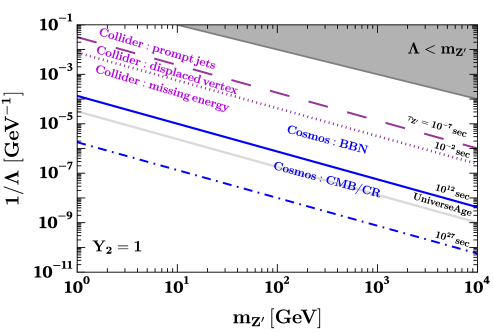
where the at-rest lifetime $\tau_{Z^{\prime}}=1/\Gamma_{Z^{\prime}}$. Fig. 1 illustrates the representative benchmark values relevant for collider phenomenology (in purple) and cosmology (in blue). In the shaded gray region of the figure there exists $\Lambda<m_{Z^{\prime}}$, where the EFT approach does not apply.

At the parton level, the three-gluon decay channel is dominant for a $Z^{\prime}$ boson with mass above 1 GeV, yielding the signatures studied below. Other potentially detectable decay channels are subject to additional suppression. For instance, $Z^{\prime}\to gg\gamma$ only happens through even higher-dimensional EFT operators within our setup, and thus is much less likely. Channels like $Z^{\prime}\to h\gamma$ and $Z^{\prime}\to\bar{f}f$ are further suppressed, as there is no intermediate beyond the SM (BSM) particles connecting $Z^{\prime}$ to electroweak interactions at tree level Bernreuther et al. (1989). At last, $Z^{\prime}\to\gamma\gamma$ is forbidden by the Landau-Yang theorem Landau (1948); Yang (1950); Chang et al. (1988); Keung et al. (2008).

As is shown by Eq. (4) and Fig. 1, the gluonic $Z^{\prime}$ boson can have a macroscopic decay length in colliders for TeV-scale $\Lambda$, leading to detectable signatures, such as missing energy and displace vertex events. This section studies such signatures at the Large Hadron Collider (LHC).

As a potentially long-lived particle, the presence of $Z^{\prime}$ at early Universe may leave imprints on cosmological observables. The most relevant constraints for our analysis are based on Big Bang Nucleosynthesis (BBN), the Cosmic Microwave Background (CMB), and the Late Universe observations; the last combines limits from low-redshift cosmic rays (CR) and the precisely-measured energy budget of the current Universe. These cosmological and astrophysical constraints will be studied and summarized in this subsection. Apparently, they could only constrain the parameter regions where $\tau_{Z^{\prime}}$ is above $10^{-2}$ sec, as the early Universe well before the BBN time cannot be reliably measured at this moment.

To quantify the effects of the $Z^{\prime}$ population on high-redshift Universe, we calculate its abundance via the associated Boltzmann equation:

where $H$ is the Hubble expansion rate, and the other three terms on the R.H.S. stand for the decay/annihilation channels of the $Z^{\prime}$ particles, together with their inverse processes. Here, $n_{i}$ and $n_{i}^{\mathrm{eq}}$ denote the actual number density and thermal equilibrium number density of the particle $i$, with respect to the photon temperature $T$. The $\sigma$ and $v_{\mathrm{Møl}}$ denote the annihilation cross section and Møller velocity, respectively, while $\langle...\rangle$ indicates thermal averaging. Note that for the third process, a factor of 2, due to the fact that each process annihilate two $Z^{\prime}$ particles, has canceled with a factor of 1/2, from double-counting of events by using $n^{2}_{Z^{\prime}}$; see Appendix C for more details. Explicit expressions of the cross sections for the processes $gZ^{\prime}\to gg$ and $Z^{\prime}Z^{\prime}\to gg$ are shown in Appendix B. The decay rate that enters the Boltzmann equation is the thermally averaged $\langle\Gamma_{Z^{\prime}}\rangle=\Gamma_{Z^{\prime}}\,K_{1}(m_{Z^{\prime}}/T)/K_{2}(m_{Z^{\prime}}/T)$, where $K_{i}$ are the modified Bessel functions of the second kind Chu et al. (2012b).

We then solve the Boltzmann equation above for $X_{1}=Y_{1}=1$ with all other operators absent. To be conservative, we take ${n}^{\text{initial}}_{Z^{\prime}}=0$ for the initial condition at the reheating temperature, $T_{\text{RH}}$. Larger values of ${n}^{\text{initial}}_{Z^{\prime}}$ would result in stronger constraints if thermalization never happens. To simplify the calculation, we neglect the $Z^{\prime}$ (semi-)annihilations into two gluons if both sectors are never thermalized with each other, and fix $T_{Z^{\prime}}$ same as the photon temperature once both sectors thermalize at some point. The two approximations are known to be reliable for such studies Chu et al. (2012b). Our numerical calculation is then performed from the reheating temperature down to $T=m_{Z^{\prime}}/100$, where the $Z^{\prime}$ production/annihilation processes necessarily decouple, and freeze-in/out should already end. For DM masses above $\mathcal{O}(1)$ GeV, the age of the Universe is still within $10^{-2}\,\text{sec}$ at this moment, and $Z^{\prime}$ becomes highly non-relativistic. That is, the $Z^{\prime}\to ggg$ decay channel can be neglected so far. In addition, we expect that annihilation via $Z^{\prime}g\to gg$ dominates over that via $Z^{\prime}Z^{\prime}\to gg$ at $T\lesssim m_{Z^{\prime}}$, where $n_{g}\gg n_{Z^{\prime}}$

The abundance $\Omega_{Z^{\prime}}$ evaluated at $T=m_{Z^{\prime}}/100$ in the $(m_{Z^{\prime}},1/\Lambda)$ plane is presented in Fig. 4 for reheating temperatures of $T_{\mathrm{RH}}=10^{5}\,\mathrm{GeV}$ (left panel) and $T_{\mathrm{RH}}=10^{7}\,\mathrm{GeV}$ (right panel). Here we ensure the EFT validity by always restricting $\Lambda>T_{\text{RH}}$. We also do not include the parameter space where $\tau_{Z^{\prime}}<10^{-2}\,\mathrm{sec}$, which is irrelevant for the cosmological probes considered in this work. This appears as the dark gray shaded region in left panel. As is well known, for portals that are described by EFT operators, the $Z^{\prime}$ population is predominantly produced around $T\simeq T_{\mathrm{RH}}\gg m_{Z^{\prime}}$, as the production processes are UV-dominated Mambrini et al. (2013). Additionally, its interaction strength with thermal bath increases with $T_{\mathrm{RH}}$. Therefore one can estimate the minimal coupling needed for two-sector thermalization by comparing the interaction rate with the Hubble rate:

at $T\simeq T_{\mathrm{RH}}$, where $M_{\mathrm{Pl}}$ is the Planck mass. Recall that at relativistic limit, there exist $\sigma_{Z^{\prime}g\rightarrow gg}v_{\mathrm{Møl}}\simeq{T^{6}/\Lambda^{8}}$ and $n_{g}^{\mathrm{eq}}(T)\simeq T^{3}$, the critical value of $\Lambda$ scales as $T_{\mathrm{RH}}^{7/8}M_{\mathrm{Pl}}^{1/8}$, being independent of the DM mass. This is shown as the horizontal solid green lines in both panels of Fig. 4, labeled as “thermalization threshold”.

Below the thermalization threshold, the $Z^{\prime}$ population never reaches thermal equilibrium with the SM sector, and thus its abundance at $T=m_{Z^{\prime}}/100$ only increases with larger couplings. Consequently, its frozen-in mass density, $Y_{Z^{\prime}}m_{Z^{\prime}}|_{T=m_{Z^{\prime}}/100}$, scales as $\propto T_{\mathrm{RH}}^{7}m_{Z^{\prime}}M_{\mathrm{Pl}}/\Lambda^{8}$, linearly dependent of mass $m_{Z^{\prime}}$. For illustration, Fig. 4 shows the three black dashed lines which correspond to $\Omega_{Z^{\prime}}=[1,10^{-10},10^{-20}]\,\Omega_{\mathrm{DM}}$, respectively. Based on the gray line in Fig. 1, we find that the $Z^{\prime}$ boson is sufficiently long-lived and, through freeze-in production, can achieve the observed relic abundance, making it a viable dark matter candidate.

For portal couplings above the thermalization threshold, the $Z^{\prime}$ particles become able to thermalize with the gluon bath around $T=T_{\text{RH}}$. Note that the interaction rate, given by the L.H.S. of Eq. (8), decreases much faster than the Hubble rate, on the R.H.S. of the equation, when the temperature drops. As a result, for the parameter regions we show in Fig. 4 the decoupling of both sectors usually happens when the $Z^{\prime}$ is still relativistic. That is, the $Z^{\prime}$ particle freezes out while being still relativistic. For such relativistic freeze-out, the frozen abundance $Y_{Z^{\prime}}$ is approximately an order-one constant, and thus the resulting mass density only depends on the the mass, as $\Omega_{Z^{\prime}}\propto m_{Z^{\prime}}$. This explains that for parameter regions above the threshold line in Fig. 4, the value of $\Omega_{Z^{\prime}}$ becomes independent of $\Lambda$. In fact, order-one values of $Y_{Z^{\prime}}$ with $\tau_{Z^{\prime}}\geq 10^{-2}\,$sec are experimentally excluded, as will be discussed shortly below.

For larger portal couplings well above the thermalization threshold, which are not fully included in Eq. (8) but are shown in Fig. 1, the $Z^{\prime}$ particle has a lifetime shorter than $10^{-2}\,$sec. Consequently, these parameter regions are safe from existing cosmological/astrophysical probes. At last, for even larger portal couplings, with $m_{Z^{\prime}}/\Lambda\gtrsim 10^{-2}$, non-relativistic freeze-out can occur and strongly suppress the frozen $Z^{\prime}$ abundance. This possibility, together with details of the freeze-in/out mechanisms, will be investigated in the next section, where the $Z^{\prime}$ particle is set to be stable.

Now we can study the observable consequences of an unstable $Z^{\prime}$ population at $T={m_{Z^{\prime}}/100}$, as given by Fig. 4, before considering a stable $Z^{\prime}$ particle in the next section. Generally speaking, its subsequent decay ejects visible energy into the thermal bath, modifying cosmological and astrophysical observables that have been measured quite precisely. In Fig. 1, blue iso-lifetime contours demonstrate the regions of cosmological and astrophysical sensitivity: BBN ($10^{-2}\,\mathrm{sec}\lesssim\tau_{Z^{\prime}}\lesssim 10^{12}\,\mathrm{sec}$) and CMB/CR ($10^{11}\,\mathrm{sec}\lesssim\tau_{Z^{\prime}}\lesssim 10^{27}\,\mathrm{sec}$). Additionally, the gray line indicates the age of the Universe, $\tau_{U}\simeq 4.3\times 10^{17}\,\mathrm{sec}$, which serves as the criterion for whether the $Z^{\prime}$ is effectively stable as a DM candidate. Since the sensitivity of each probe depends on the $Z^{\prime}$ lifetime, we use complementary experimental and cosmological observations to constrain the combination of $(m_{Z^{\prime}},1/\Lambda)$ parameters. In what follows, we describe in detail how each of these probes constrains the parameter plane.

BBN. The BBN theory successfully predicts the primordial abundances of light elements, while late-decaying $Z^{\prime}$ particles may disrupt these predictions through hadronic energy injections that alter the $n/p$ ratio or induce hadro-dissociation of light nuclei. Recent searches use primordial abundance measurements of deuterium, helium-3/4, and lithium-7 to place strong constraints on the primordial abundance of BSM particles decaying into the SM bath, with lifetimes between $\tau=10^{-2}\,\mathrm{sec}$ and $10^{12}\,\mathrm{sec}$ Kawasaki et al. (2005); Angel et al. (2025). Therefore, we adopt their results to constrain the $(m_{Z^{\prime}},1/\Lambda)$ plane by requiring the primordial $Z^{\prime}$ abundance calculated above to lie below the observational upper bounds.

CMB. The injection of high–energy electromagnetic particles around recombination modifies the recombination history and hence the CMB anisotropy power spectra. Accounting for delayed energy deposition, there are many studies that place stringent limits on the abundance of late–decaying BSM particles with lifetimes $\tau\sim 10^{11}\text{–}10^{24}\,\mathrm{sec}$. In our setup, $Z^{\prime}$ decays predominantly via $Z^{\prime}\!\to ggg$; the ensuing hadronization rapidly yields photons and charged leptons (e.g., via $\pi^{0}\!\to\gamma\gamma$). Accordingly, we assume that most of the energy injected by $Z^{\prime}$ decay is electromagnetic and, for each $\tau_{Z^{\prime}}$, require the $Z^{\prime}$ relic abundance to satisfy the corresponding CMB bounds in Ref. Acharya and Khatri (2019), thereby constraining the $(m_{Z^{\prime}},\,1/\Lambda)$ plane.

Late Universe (CR + relic abundance). For lifetimes exceeding the age of the Universe ($\tau_{Z^{\prime}}>\tau_{U}$), the $Z^{\prime}$ is effectively stable on cosmological timescales and can constitute a DM component. In this case, CR data constrain the injected hadronic power from dark–matter decay. Under the conservative assumption of purely hadronic decays, CR observations imply an approximately mass–independent lower bound on the lifetime for single–component DM, $\tau_{\rm DM}\gtrsim 10^{27}\,\mathrm{sec}$, over the mass range relevant this work Paopiamsap et al. (2024); Ackermann and others (2012). Since the constrained quantity is the injected power $P_{\rm inj}\propto\Omega_{Z^{\prime}}/\tau_{Z^{\prime}}$ in the limit of $\tau_{Z^{\prime}}\gg\tau_{U}$, such observations can also be re-scaled to constrain a sub-leading component of the DM abundance via

In addition, we impose the relic-density bound $\Omega_{Z^{\prime}}h^{2}\leq\Omega_{\rm DM}h^{2}\simeq 0.12$, as measured by Planck Aghanim and others (2020). We refer to the CR and relic abundance bounds collectively as the late–Universe constraint.

The resulting exclusion limits are displayed as distinct blue shaded regions, corresponding to the BBN, CMB and late-Universe probes, in the left (right) panel of Fig. 5 for $T_{\mathrm{RH}}=10^{5}\,\mathrm{GeV}$ ($T_{\mathrm{RH}}=10^{7}\,\mathrm{GeV}$), respectively. Note that, in deriving the cosmological constraints, we discard the part of the cosmologically relevant parameter space where the EFT condition $\Lambda\gtrsim T_{\mathrm{RH}}$ is violated, since our EFT approach does not provide reliable predictions there. However, the collider bounds obtained in Sec. 3.2 remain reliable, as they probe much lower energy scales where the EFT description can be mostly considered as valid.

In both panels of Fig. 5, the dashed orange line denotes the single–component DM condition, $\Omega_{Z^{\prime}}=\Omega_{\mathrm{DM}}$. Its physical meaning is clarified in Fig. 4, where this line separates the region with $\Omega_{Z^{\prime}}>\Omega_{\mathrm{DM}}$ (above the line) from that with $\Omega_{Z^{\prime}}<\Omega_{\mathrm{DM}}$ (below the line) at the time where $T=m_{Z^{\prime}}/100$. In the left panel of Fig. 5 with $T_{\text{RH}}=10^{5}\,$GeV, we infer that the $Z^{\prime}$ can account for the entirety of the DM abundance only for $m_{Z^{\prime}}\lesssim 200\,\mathrm{GeV}$. Above this mass, indirect searches Paopiamsap et al. (2024); Ackermann and others (2012) require $\Omega_{Z^{\prime}}<\Omega_{\mathrm{DM}}$, implying that the $Z^{\prime}$ can only constitute a subdominant fraction of the DM abundance, otherwise its decay would lead to gamma-ray excess beyond the current experimental limit. Similarly, CMB data Acharya and Khatri (2019) imposes upper limits on the primordial $Z^{\prime}$ abundance that intersects the single–component DM contour at $\tau_{Z^{\prime}}\sim 10^{24}\,\mathrm{sec}$. For shorter lifetimes, these constraints become increasingly stringent, forcing $\Omega_{Z^{\prime}}<\Omega_{\mathrm{DM}}$ until $\tau_{Z^{\prime}}\simeq 10^{12}\,\mathrm{sec}$. Complementarily, BBN data Kawasaki et al. (2005); Angel et al. (2025) provide the leading constraints for $Z^{\prime}$ particles with lifetime between $10^{-2}$ and $10^{12}$ sec, requiring $\Omega_{Z^{\prime}}<\Omega_{\mathrm{DM}}$ in this region. This is the reason why, above the dotted orange line of $\Omega_{Z^{\prime}}=\Omega_{\mathrm{DM}}$ line, the combination of BBN and CMB exclude all the parameter regions for lifetime $10^{-2}\,\mathrm{sec}\lesssim\tau_{Z^{\prime}}\lesssim 10^{12}\,\mathrm{sec}$ and $10^{12}\,\mathrm{sec}\lesssim\tau_{Z^{\prime}}\lesssim 10^{24}\,\mathrm{sec}$, as indicated in Fig. 1.

At last, we emphasize that for the line of $\Omega_{Z^{\prime}}=\Omega_{\mathrm{DM}}$ in Fig. 5, the observed DM relic abundance can be produced via pair annihilation of SM gluons. Its location relies on the reheating temperature. For the left panel with $T_{\text{RH}}=10^{5}\,$GeV, the lifetime of $Z^{\prime}$ is too short to satisfy the current CMB and CR bounds if $m_{Z^{\prime}}>200$ GeV, but the region for lighter $Z^{\prime}$ is not constrained by observations, except for the argument that its current density should not exceed the observed DM density. That is, $Z^{\prime}$ can play the role of the dominant DM candidate, and a successful production via the freeze-in mechanism is allowed. It happens for $m_{Z^{\prime}}\leq 200\,$GeV in the case of $T_{\text{RH}}=10^{5}\,$GeV, and applies to the whole ${Z^{\prime}}$ mass region considered here if $T_{\text{RH}}=10^{7}\,$GeV, as shown in the right panel of Fig. 5. This is because, in the freeze-in mechanism, higher reheating temperatures correspond to smaller couplings, which result in longer-lived $Z^{\prime}$ particles. These longer lifetimes help alleviate the CMB and CR bounds, thereby allowing for a wider ${Z^{\prime}}$ mass range to account for the whole observed DM abundance.

In the freeze-in mechanism McDonald (2002); Choi and Roszkowski (2005); Kusenko (2006); Petraki and Kusenko (2008); Hall et al. (2010), SM particles are produced directly from the inflaton decay and form a thermal bath first, while the DM particles, the $Z^{\prime}$ bosons in our model, reside in a dark sector and are initially absent at the end of the inflation. Through feeble portal interactions induced by the operators $\mathcal{O}_{1-4}$, the population of $Z^{\prime}$ particles are later generated via out-of-equilibrium processes from the SM bath, such as gluon fusion

eventually yielding the observed relic abundance. As a special case of Eq. (3.3), the corresponding Boltzmann equation that describes the freeze-in evolution of $n_{Z^{\prime}}$ can be obtained by omitting contributions of $\mathcal{O}_{5,6}$ and inverse processes as follows:

where $R(T)$ denotes the $Z^{\prime}$ production rate. More explicit expressions for these quantities are provided in Appendix D. In contrast to IR-dominated freeze-in scenario, where the DM production proceeds through renormalizable operators and is insensitive to the reheating temperature $T_{\text{RH}}$, our setup involves $Z^{\prime}$ production via non-renormalizable dimension-8 operators, corresponding to a UV-dominated freeze-in mechanism; see Bernal et al. (2017) and references therein. In this case, DM particles are predominantly produced just after reheating, rendering the final abundance highly sensitive to $T_{\text{RH}}$. In order to make the EFT description valid, we always require that $T_{RH}$ is much smaller than the cut-off energy scale $\Lambda$. The present-day frozen-in yield, defined as $Y_{Z^{\prime},0}\equiv n_{Z^{\prime},0}/s_{0}$, where $n_{Z^{\prime},0}$ is the present-day number density of $Z^{\prime}$ and $s_{0}$ is the present-day entropy density, thus admits an analytical expression:

where $g_{*}^{S}(T)$ and $g_{*}^{\rho}(T)$ denote the effective numbers of relativistic degrees of freedom for entropy and energy densities, respectively. The dimensionless function $F_{1}(\{X_{j}\})$ encodes the dependence on the Wilson coefficients $X_{j}$. The derivation of Eq. (12) and the explicit form of $F_{1}(\{X_{j}\})$ are provided in Appendix D. For numerical results, the yield can be approximated as

The left panel of Fig. 6 illustrates the evolution of $Y_{Z^{\prime}}$ during the freeze-in process for a benchmark scenario in which only $X_{1}=1$ contributes (i.e., $F_{1}(\{X_{j}\})=64$), with $\Lambda=1.26\times 10^{10}~\mathrm{GeV}$, $m_{Z^{\prime}}=10^{4}~\mathrm{GeV}$, and $T_{\mathrm{RH}}=10^{7}~\mathrm{GeV}$. The expected yield, $Y_{Z^{\prime},0}=4.1\times 10^{-14}$, for this benchmark scenario, computed according to Eq. (13), is indicated by the horizontal blue line. For comparison, the gray dashed line indicates the corresponding thermal equilibrium abundance, $Y_{Z^{\prime}}^{\rm EQ}$. The evolution obtained from numerical integration and from the analytical approximation is represented by the black dashed and red solid lines, respectively. The excellent agreement between these two results confirms the validity of the analytical expression, and the final yield is consistent with the observed DM relic abundance.

Then, by requiring that the $Z^{\prime}$ population saturates the observed DM relic abundance, $\Omega_{Z^{\prime},0}h^{2}\simeq 0.12$, corresponding to $m_{Z^{\prime}}\,Y_{Z^{\prime},0}\simeq 4.1\times 10^{-10}\,\text{GeV}$, as measured by the Planck Collaboration Aghanim and others (2020), we derive the corresponding values of $1/\Lambda$ as a function of the mediator mass $m_{Z^{\prime}}$. For illustration, we consider two benchmark reheating temperatures, $T_{\mathrm{RH}}=10^{5}~\mathrm{GeV}$ and $10^{7}~\mathrm{GeV}$, and assume that only the Wilson coefficient $X_{1}=1$ contributes (i.e., $F_{1}(\{X_{j}\})=64$). These are shown in right panel of Fig. 7 by solid (dashed) orange lines for $T_{\mathrm{RH}}=10^{5}$ ($10^{7}$) GeV. In both cases, the resulting $1/\Lambda$ values remain within the regime of EFT validity, i.e., $\Lambda>T_{\mathrm{RH}}$.

The freeze-out mechanism is a widely studied framework for explaining the DM relic abundance; see e.g.  Scherrer and Turner (1986); Kolb and Turner (2019); Gondolo and Gelmini (1991). Unlike the freeze-in mechanism above, where the observed DM abundance is produced out-of-equilibrium, the freeze-out mechanism assumes that DM was initially in equilibrium. As the Universe expanded and cooled, DM particles eventually decoupled from the thermal bath, freezing their comoving number density. With a residual $\mathcal{Z}_{2}$ symmetry, the number density of $Z^{\prime}$ is governed by the Boltzmann equation (Eq. 3.3) through the $Z^{\prime}Z^{\prime}\leftrightarrow gg$ channel:

where the thermally-averaged cross section $\langle\sigma v_{\mathrm{Møl}}\rangle_{Z^{\prime}Z^{\prime}\to gg}$ can be calculated from Gondolo and Gelmini (1991):

where $T$ is the photon temperature and $K_{1,2}$ are modified Bessel functions of the second kind. The explicit form of $\sigma_{Z^{\prime}Z^{\prime}\to gg}$ is given in Appendix B.

We numerically compute the thermal evolution of the $Z^{\prime}$ relic abundance and require that its present value matches the observed DM abundance $\Omega_{Z^{\prime},0}h^{2}\simeq 0.12$, within the benchmark scenario where only $X_{1}=1$ contributes. The result is shown in right panel of Fig. 6 for $m_{Z^{\prime}}=10^{4}\,\mathrm{GeV}$ and $\Lambda=1.51\times 10^{4}\,\mathrm{GeV}$. In the plot, the red solid line represents the time-evolved relic abundance $Y_{Z^{\prime}}$, the red dashed line corresponds to its thermal equilibrium abundance $Y_{Z\prime}^{EQ}(T)$, and the horizontal blue solid line indicates the observed DM abundance $Y_{Z^{\prime},0}$. The general freeze-out annihilation cross section, $\langle\sigma v_{\mathrm{M\o l}}\rangle_{Z^{\prime}Z^{\prime}\to gg}$, required to reproduce the observed DM relic abundance, as a function of $m_{Z^{\prime}}$ is illustrated as the dotted red line in the left panel of Fig. 7. The obtained values are close to the typically canonical one, $10^{-36}\,\mathrm{cm}^{2}$. In turn, the couplings needed to generate the observed DM relic abundance, as a function of the DM mass $m_{Z^{\prime}}$, is shown as the solid red line in the right panel of Fig. 7.

Direct detection of DM relies on observing stable nuclear (electron) recoils resulting from elastic DM–nucleus (electron) scattering processes. Thus the null results from recent direct detection experiments Aalbers and others (2024); Li and others (2023); Acerbi and others (2024) place upper limits on the spin-independent DM–nucleon scattering cross-section. For $Z^{\prime}$ with $m_{Z^{\prime}}\gtrsim 1\,\mathrm{GeV}$ and a typical Galactic speed $v\sim 10^{-3}c$, $Z^{\prime}$–nucleon scattering is non-relativistic, with the maximal momentum transfer, $q=2\,\mu_{Z^{\prime}n}\,v$, set by the reduced mass,

where $m_{n}\simeq 0.94~\mathrm{GeV}$ denotes the nucleon mass, and the factor of 2 corresponds to backward scattering (maximal nucleon recoil).

Since $q\ll\Lambda_{\rm QCD}$, the interaction must be described in terms of nucleon matrix elements rather than partonic perturbation theory. Accordingly, computing the spin-independent cross section $\sigma^{\rm SI}_{Z^{\prime}N}$ requires matching the partonic operators $\mathcal{O}_{1\text{--}4}$ onto nucleon-level operators. Recent studies on such matching procedures can be found in Refs. Fitzpatrick et al. (2013); Bishara et al. (2017a, b), though only the matching of the partonic operator $\mathcal{O}_{1}$ has been thoroughly studied in these works. Generally, according to power counting, the other operators contribute to the same order of magnitude as $\mathcal{O}_{1}$. So we first consider the case with $X_{1}=1$ and all other Wilson coefficients set to zero, as illustration. In the non-relativistic limit, the spin-independent $Z^{\prime}$–nucleon scattering cross-section is

where $m_{G}\simeq 848~\mathrm{MeV}$ denotes the gluonic contribution to the nucleon mass in the isospin-symmetric limit and $\alpha_{s}\simeq 0.118$ is the QCD coupling constant Bishara et al. (2017b). The detailed derivation of $\sigma_{Z^{\prime}n}^{\rm SI}$ can be found in Appendix B. We combine the latest results from LZ Aalbers and others (2024), PandaX-4T Li and others (2023), and DarkSide-50 Acerbi and others (2024) to obtain upper bounds on $\sigma_{Z^{\prime}n}^{\rm SI}$, as demonstrated by the purple solid line in the left panel of Fig. 7. The corresponding direct-detection constraints on $1/\Lambda$, obtained by requiring $\sigma_{Z^{\prime}n}^{\mathrm{SI}}$ to lie below this bound, are shown as purple regions in the right panel of Fig. 7. These results exclude the thermal freeze-out mechanism for $m_{Z^{\prime}}\lesssim 1~\text{TeV}$.

Recasting precisely the constraints for the other operators is non-trivial. Instead, we compute the relevant partonic-level cross sections (mostly importantly, $Z^{\prime}g\to Z^{\prime}g$) induced by the operators $\mathcal{O}_{2-4}$, and find that their contributions are of the same order as that from $\mathcal{O}_{1}$ at non-relativistic limit. For simplicity, we therefore assume that the $Z^{\prime}N\to Z^{\prime}N$ scattering cross sections induced by $\mathcal{O}_{2-4}$ are of the same order as that by $\mathcal{O}_{1}$. Based on this, we believe that direct detection bounds on $\Lambda$ for $\mathcal{O}_{2-4}$ are comparable, due to the high exponent on $\Lambda$ in the scattering cross sections.

While $Z^{\prime}$ pair annihilation becomes highly suppressed with the expansion of the Universe, and has a negligible impact on the relic density, its annihilation at high-redshifts and local dense regions can still product a lot of gluons, or neutral/charged pions after hadronization. This would potentially lead to excesses of gamma-ray, anti-proton, and high-energy neutrinos, beyond the predictions of standard astrophysics; see e.g. Bertone et al. (2005); Cirelli et al. (2011); Chu et al. (2012a); Abbasi and others (2023). Therefore, observational data from gamma-ray and cosmic-ray observatories, such as the High Energy Stereoscopic System (H.E.S.S.) Hinton (2004), Alpha Magnetic Spectrometer (AMS-02) Aguilar and others (2016), and the Fermi-LAT telescope Atwood and others (2009), can be used to place upper limits on the DM annihilation cross section at various masses.

For illustration, we again adopt the parameter choice where $X_{1}=1$, while setting all other Wilson coefficients to vanish. In this case the DM annihilation cross section at the non-relativistic limit can be written as

We combine the latest bounds on the upper bounds on $\left\langle\sigma_{Z^{\prime}Z^{\prime}\rightarrow gg}v_{\mathrm{M\o l}}\right\rangle$ from the H.E.S.S. Abdalla and others (2022) and Fermi-LAT Paopiamsap et al. (2024) collaborations, as given by the green solid line in the left panel of Fig. 7. The corresponding exclusions on our $1/\Lambda$ are then given as the green regions at the top-right corner of the right panel of Fig. 7. For DM annihilation dominantly into gluons, thermal freeze-out is only experimentally allowed for the $Z^{\prime}$ mass above tens of GeV, in agreement with previous studies Elor et al. (2016); Bartlett et al. (2022).

In the DM scenario, the $Z^{\prime}$ can be produced at the LHC but gives rise only to missing–energy signatures through the $2\to 3$ process $pp\to Z^{\prime}Z^{\prime}j$. In contrast to the general case discussed in Sec. 3.2.1, we here omit the probability factor $\mathcal{P}_{D}(L_{1},L_{2})$, and impose the DM $Z^{\prime}$ does not decay inside the detector. That is, the relevant signal cross section is simply

whose numerical values has already been given in the left panel of Fig. 3 as a function of $m_{Z^{\prime}}$. Considering the case $X_{1}=1$, we impose the same requirement $\sigma_{\rm sig}<0.3~\mathrm{fb}$ Aad and others (2021) as before, and obtain the missing–energy constraints as the light gray shaded regions in the right panel of Fig. 7.

Before ending this section, we briefly comment on other potential probes of such a DM abundance, such as its capture in stars and consequent effects. For instance, in a DM-dense environment, the processes $Z^{\prime}Z^{\prime}\to gg$ and $Z^{\prime}g\to Z^{\prime}g$ in a neutron–star core could in principle modify the stellar evolution. For the small effective couplings (large $\Lambda$) considered here , the corresponding rates are parametrically suppressed due to the low centre-of-mass energy, and are not expected to yield competitive constraints, so we do not further consider them here.