Vanishing for Hurwitz spaces of fully-marked admissible covers of degree 3
Abstract.
We show that the first cohomology group of the Hurwitz space of fully-marked admissible covers vanishes for covers of degree and deduce the same result for the classical Hurwitz space of simply-branched covers. In degree 4, we compute examples where is nonzero, which implies that is nonvanishing for . We describe the stratification of the boundary of by lower-dimensional , and set up an inductive framework which may be used for future arguments involving the odd cohomology of .
2020 Mathematics Subject Classification:
14H10, 14H30, 14C171. Introduction
The Hurwitz space parametrizes simply-branched degree- covers from smooth connected genus- curves to smooth genus- curves, marked at branch points. Harris and Mumford introduced the “admissible covers” compactification of , in which the target and source curves of a cover degenerate to nodal curves as branch points come together and the target curve is stable [HM82]. Although this space is singular, its normalization is the smooth moduli space of twisted stable maps [ACV03], which we denote by . We refer to the normalization whenever we mention the admissible covers compactification. The Picard Rank Conjecture [DE96] predicts that the rational Picard group vanishes in all degrees for both and its variant . Recent work on the geometry of confirms this conjecture for [DP15] and for [MUL23]. Furthermore, the homology of stabilizes, implying that the Picard Rank Conjecture holds asymptotically when [LL25].
The Hurwitz space of degree-2 admissible covers is isomorphic to the quotient . It follows that . For admissible covers of degree 3, we develop tools for an inductive argument inspired by [AC98] to show that vanishes for the Hurwitz space of fully-marked admissible covers , a generalization of . This Hurwitz space parametrizes possibly disconnected admissible covers with fully-marked fibers of prescribed (not necessarily simple) ramification (see 2.1).
Theorem 1.1.
The first cohomology group for every partition of , every partition of , and any set of ramification profiles partitioning .
We give examples of 1-dimensional Hurwitz spaces in degree 4 and degree 5 of fully-marked admissible covers with positive genus (see Section 6.3). It follows that does not vanish for .
The spaces and are finite group quotients of , where the source curve is connected and all marked fibers have simple ramification (see Section 2.1). We immediately obtain the following corollary.
Corollary 1.2.
The first cohomology groups .
Our proof of Theorem 1.1 is inspired by the inductive argument introduced by Arbarello and Cornalba to study the low degree odd cohomology of moduli spaces of stable curves [AC98]. Arbarello and Cornalba used the stratification of the boundary of by the images of gluing maps from products of lower-dimensional moduli spaces of curves to show that vanishes for and . They conjectured that inductive arguments could be used to show vanishing for higher odd , once the requisite base cases were proven. Indeed, Bergström, Faber, and Payne showed that vanishes for and [BFP24], thereby proving the conjecture for all odd . This bound is optimal, since the cohomology group is nonzero once .
Adapting these strategies to Hurwitz spaces requires new tools. First, we must find a Hurwitz space with the correct boundary structure. Like , the boundaries of the simply-branched Hurwitz spaces and are stratified by the images of gluing maps from products of lower-dimensional Hurwitz spaces. The Hurwitz spaces appearing in the domains of these gluing maps, however, parametrize admissible covers with arbitrary (not necessarily simple) ramification, since a simply-branched admissible cover in the boundary may have arbitrary ramification over the nodes. Thus, even if we are primarily interested in the low degree odd cohomology of and , in order to argue inductively we are inevitably led to study the low degree odd cohomology of the more general Hurwitz spaces .
In Proposition 5.2, we show that when is odd, the vanishing of the -th cohomology group of low-dimensional implies the vanishing of the -th cohomology group for all . Thus, for and , we must compute for every possible choice of ramification profile . To solve this technical challenge, we take advantage of the natural target map from these 1-dimensional Hurwitz spaces to , which is a covering map. For each base case, it suffices to compute the monodromy of this target map, thereby computing that each Hurwitz space is genus-0. Theorem 1.1 follows.
In principle, Proposition 5.2 could be used to prove vanishing for higher odd , analogously to the argument in [AC98]; see Remark 5.3.
1.1. Outline of the paper
In Section 2, we define Hurwitz spaces of fully-marked admissible covers and describe their relationships to other Hurwitz spaces in the literature. In Section 3, we recast the geometric data of an admissible cover as the combinatorial data of monodromy representations, allowing us to combinatorially describe the target map . In Section 4, we show that the boundary divisors of are finite quotients of products of lower-dimensional Hurwitz spaces, setting the stage for the inductive proof of vanishing in Section 5. Finally, in Section 6, we record the data of the base cases necessary to prove that vanishes for admissible covers in degrees 3. We also provide examples of 1-dimensional Hurwitz spaces of fully-marked admissible covers in degrees 4 and 5 which have positive genus.
Acknowledgements
The author would like to thank Chiara Damiolini, Darragh Glynn, Rok Gregoric, Rohini Ramadas, Kenny Schefers, and Sara Torelli for helpful conversations related to this project. Special thanks to Hannah Larson for valuable discussions about computing the 1-dimensional base cases, as well as helpful comments on an earlier version of this paper. Finally, the author would like to thank their advisor, Sam Payne, for guiding them to an interesting problem and for many productive conversations. The author was supported in part by NSF DMS–2542134.
2. Fully-marked admissible covers
Here, we define the Hurwitz spaces in this paper and describe their relationships to other Hurwitz spaces in the literature.
Definition 2.1 (Fully-marked admissible covers).
Let be a partition of an integer . Let be a tuple of nonnegative integers. Let be a tuple of partitions of where each . A fully-marked admissible cover of type is a finite morphism satisfying the following:
-
•
The target curve is an -marked stable curve of genus 0.
-
•
The source curve is a disjoint union of stable curves of genus , marked at each point in the inverse image of the marked locus of . The map has degree .
-
•
The fibers over the marked points of satisfy the ramification profiles given by the . Precisely, if is a marked point on with ramification profile , then . Consequently, points in with the same ramification profile are distinguished by the marking.
-
•
The nodes of are the inverse image of the nodes of . At a node, the cover is locally given by on both branches of the node for some (known as the kissing condition).
-
•
The map is étale outside of the marked locus and nodes of .
We define families of fully-marked admissible covers as follows.
Definition 2.2.
A family of fully-marked admissible covers of type over a scheme is a commutative diagram
where:
-
•
The target curve is a genus- curve over with sections .
-
•
The source curve is a disjoint union of stable genus- curves over , with sections satisfying . The map has degree .
-
•
is étale outside of the image of the and the nodes of .
Definition 2.3 (Morphisms of fully-marked admissible covers).
A morphism of families of fully-marked admissible covers of type from to over is a pair of morphisms such that the diagram below commutes:
Definition 2.4 (Hurwitz space of fully-marked admissible covers).
Let be a partition of an integer . Let be a tuple of nonnegative integers. Let be a tuple of partitions of where each .
The Hurwitz space is the moduli stack of isomorphism classes of fully-marked admissible covers of type . There is an open dense substack parametrizing such admissible covers where and are smooth. When and , corresponding to connected covers, we simply write .
Remark 2.5.
The Hurwitz space defined in Definition 2.4 is a generalization of the admissible covers compactification of . The geometric picture to have in mind is that when marked fibers approach each other, they “bubble off” onto another component (simultaneously on the source and target curves). A helpful discussion of this appears at the end of Chapter 3, Section 3 in [HM06].
2.1. Relation to other Hurwitz spaces
The Hurwitz space of fully-marked admissible covers is the same as the Hurwitz space treated in [CMR14], except that here we fix the target curve to be genus-0.
In [ACV03], Abramovich, Corti, and Vistoli introduced the space parametrizing arbitrarily branched covers from possibly disconnected source curves with marked points on the target genus-0 curve, and showed that it is a smooth stack. Here, we use (slightly differing from the notation of [ACV03]) to denote the degree of the cover from the different components of the source curve. The space has a covering map from given by quotienting by where is the product of symmetric groups corresponding to repeated ramification indices in . For example, the ramification profile corresponds to the product . Quotienting by corresponds to forgetting the ordering in each marked fiber on the source curve. In particular, this covering map is étale, since its fibers have constant cardinality. Therefore is also smooth (as a stack).
We denote the Hurwitz space of connected, fully-marked, simply-branched covers by
where . When , only the branched fibers are marked. The Harris-Mumford Hurwitz space introduced in [HM82] is the quotient , which we denote by . Finally, the Hurwitz space specified in the Picard Rank Conjecture (see [DP15, MUL23]) is the quotient , which we denote by .
The Hurwitz spaces are the ones discussed in [Sv20] and [FP05]. We denote the connected admissible covers of [ACV03] by . As varies, the collection of stratifies the Hurwitz spaces discussed in [CL22] and in [ZHE22]. In those papers, they work with unmarked, arbitrarily branched covers, so branch points are allowed to collide.
3. Fully-Marked Monodromy representations
The geometric data of a degree- admissible cover can be recast as the combinatorial data of monodromy representations. This provides an alternative perspective on Hurwitz spaces relying only on combinatorial data, making explicit computations easier.
First, we define families of labeled admissible covers.
Definition 3.1.
(Labeled admissible covers). A family of labeled admissible covers of type over a scheme is the data of a fully-marked admissible cover as in Definition 2.1, along with a diagram
where:
-
•
The section lies in the smooth locus of and is disjoint from all marked points on .
-
•
The sections on satisfy .
We call these sections the labeling of , and the tuple a labeled admissible cover.
To construct a monodromy representation associated to a labeled admissible cover, we fix the following:
-
•
Let be a closed point, and consider a labeled admissible cover over .
-
•
Fix an isomorphism such that the first three marked points of the marked locus are sent to and .
-
•
Fix a generating set for where is a loop based at winding around once in the clockwise direction.
For any in the generating set for , consider its lift to a path in starting at , i.e. . The other endpoint of this lift must also lie in . Define by where . Observe that the cycle type of is exactly the ramification profile of at . For each , we can associate such a permutation , producing a homomorphism . We package the data of this homomorphism by the ordered tuple . Finally, we keep track of the marking on by marking the cycles in each of the . For example, in Figure 1, the ramification point has profile . Given the labeling on , the associated permutation to is , where is marked as , is marked as and is marked as .

Then the fully-marked monodromy representation of the labeled admissible cover consists of
-
(1)
a monodromy representation , and
-
(2)
a marking on the cycles in each permutation .
Two labeled admissible covers and are isomorphic if there is an isomorphism between the fully-marked admissible covers and (see Definition 2.3) such that . Isomorphic labeled admissible covers have identical monodromy representations, by the following argument. Let be any generator of . Let and be the permutations associated to lifting via and , respectively. Then, for any , we have that is defined by and is defined by . Applying to the first equation, we find that:
This last step follows since is an isomorphism and the lifts and are continuous. Therefore . For this reason, if two labelings of differ by an automorphism of , then they have identical monodromy representations.
In general, given any two labelings and for , the pairs and have “simultaneously conjugate” monodromy representations. This means that if and have the monodromy representations and respectively, then there exists some such that for every . In this case, we have . Furthermore, the markings on and have the following relationship: the marking on the cycle of is equal to the marking on the cycle of . For example, in Figure 1, the fiber over is associated to the permutation in terms of the labeling , with markings respectively.
Let the simultaneous conjugacy class be the set of all tuples which are simultaneously conjugate to . Due to the relation in , the set must satisfy . If the admissible cover is connected, then acts transitively on . By the previous discussion, the isomorphism class in the Hurwitz space can be associated to .
Conversely, given a tuple of permutations from which multiply to the identity and a marking on the cycles in each , one can construct a fully-marked admissible cover of . We give an idea of the construction here. Pick some representative . Consider the polygon resulting from choosing and cutting along simple paths from to each of the branch points in . Take copies of and denote them by . Denote the sides of polygon corresponding to the path from to by . We glue these polygons together using via the following rule: the side on should be glued to the side on . This results in a (possibly disconnected) punctured surface which smoothly covers with degree . The Riemann existence theorem guarantees the existence of a unique map of Riemann surfaces which extends this covering over the punctures (see Proposition 1.2 of [FUL69]). We then add markings in the natural way: over a (filled-in) point in the target curve, we have as many points as there are cycles in . Each point corresponds to a cycle, so it inherits the cycle’s marking . As discussed previously, any simultaneous conjugate of results in the same cover of Riemann surfaces, since it corresponds to choosing a different labeling.
3.1. The target map
There is a natural target map sending an admissible cover to the target curve marked at points. This is a covering map, ramified over the boundary, whose generic fiber at a point is the set of isomorphism classes of fully-marked admissible covers which have marked locus . Once we fix generators for , we have a bijection between the points in this fiber and the set of simultaneous conjugacy classes of fully-marked monodromy representations whose permutations have cycle type equal to the prescribed ramification profiles and multiply to the identity. Consequently, the sheets of the Hurwitz space above can be identified with these fully-marked monodromy representations. This helps us calculate the monodromy of the target map, which we carry out in Section 5.3.2.
4. The boundary divisors of
In this section, we explain why the boundary divisors of are finite group quotients of products of lower-dimensional .
First, we relate the boundary of the Hurwitz space with the boundary of . The target map sends boundary divisors of to the boundary divisors of . The divisor parametrizes genus-0 curves consisting of two components connected by a single node, with marked points on one component and marked points on the other component (see the lower graph in Figure 2 for the dual graph of ). There are multiple isomorphic components in , corresponding to the different labelings of the marked points. Above , the boundary divisors of parametrize admissible covers of where the fibers over the marked points have the ramification profiles . On each component of , the permutations associated to the marked points and the node must multiply to the identity. Therefore, the ramification profile over the node is constrained by the ramification profiles of the fibers over the marked points on either component. We can associate a dual graph to an admissible cover by taking the usual dual graph construction of a marked curve for both the source and target curves (see details in Section 3.2 of [CMR14]). Additionally, we label the edges and half-edges in the source graph with the ramification index. In this way, every boundary divisor in the Hurwitz space has a dual graph of admissible covers , and we refer to such a boundary divisor by . There may be multiple above each component of , as in Figure 2.

There are natural gluing maps
| (1) |
associated to each such that are partitions of and , where is the length of . The gluing map is given by specifying that marked points should be identified if they correspond to an edge in the dual graph. Then is the quotient of the image of by the group of graph automorphisms . For example, the divisor in Figure 2 is the quotient of the image of the gluing map by , since there are -many ways to choose the labelings on the preimage of the glued fiber.
Remark 4.1.
Examining the analogous gluing maps to the boundary of illustrates how is not stratified by lower-dimensional , but rather by Hurwitz spaces of possibly disconnected, arbitrarily-branched admissible covers with some number of marked fibers. For example, the Hurwitz spaces in the domain of the gluing maps to the boundary divisors of parametrize covers with one marked fiber. As the codimension of the boundary stratum increases, more marked fibers are necessary to define the gluing maps. Consequently, any inductive proof of odd cohomology vanishing for in the style of Theorem 1.1 necessarily involves studying the more general spaces .
5. Vanishing of
In this section, we prove that the cohomology of injects into the cohomology of the normalization of the boundary whenever it injects into the cohomology of the boundary (Lemma 5.1). We use this result to prove that the odd cohomology of vanishes for all and if certain base cases have this property (Proposition 5.2). We apply this argument for and explain how to compute the base cases.
5.1. Injectivity of pullback map on cohomology
Recall that the target map is a finite cover (see Section 3.1). As is affine of dimension , it follows that is also affine of dimension . Therefore the homology groups vanish for , and by Poincaré duality, the compactly supported cohomology vanishes for . The long exact sequence for compactly supported cohomology is as follows:
Hence the map is injective when . Now we show that also injects into the cohomology of the normalization of the boundary in this range.
Lemma 5.1 (Injectivity lemma).
Let be the gluing map associated to the boundary divisor parametrizing admissible covers with dual graph , where each is a product . If is injective, then the map is injective, where the direct sum is taken over all boundary divisors.
Proof.
Let be the disjoint union of the gluing maps . It is a proper and surjective map. Similarly to the discussion for in [AC98, Prop. 2.7], the weight quotient
is the image of under . Therefore we can factor as in the following diagram:
To show that is injective, it suffices to show that is injective on the image of . As is a restriction map, it is a morphism of mixed Hodge structures and must respect the weight filtration. Furthermore, the cohomology is pure weight , since is smooth. Hence the intersection is zero. ∎
5.2. Inductive vanishing of odd cohomology
Proposition 5.2.
Let be an odd integer. Suppose that for all odd and parameters such that . Then for all odd and all parameters .
Proof.
We induct on . Assume the claim is true for all and all parameters . We need to show that for all with .
Lemma 5.1 holds in this range, so is injective. Each space is a product where are partitions of and . Crucially, the number of marked fibers on each factor of the domain is strictly less than . By the Künneth formula, the cohomology groups decompose as
As is odd, there must be a factor with odd cohomological degree in each summand. These factors with odd degree strictly less than vanish via the induction hypothesis, and therefore is a direct sum of tensor products where and are either or 0.
If , then . Otherwise and one applies the previous argument again to get an injection into a direct sum of tensor products of and , with . The same reasoning holds for . By iterating this argument, eventually becomes larger than etc., and then . Therefore . ∎
Remark 5.3.
We use Proposition 5.2 to prove vanishing for in this paper. As the analogous proposition for was used to prove vanishing of odd cohomology in higher degree, it may be possible to do the same for . Since the number of base cases grows with the cohomological degree, a successful proof would likely involve calculating Euler characteristics and a robust understanding of the combinatorics of the boundary strata of .
5.3. Computing for degree- covers
As discussed in Section 5.1, the map is injective for all . In particular, is injective whenever , i.e. whenever the target curve has or more marked points. To show that using Proposition 5.2 for , we must show that for every Hurwitz space of admissible covers with or marked fibers. As Hurwitz spaces with marked fibers are 0-dimensional, we are left with the 1-dimensional spaces. In this section, we describe how to compute the genera of these 1-dimensional Hurwitz spaces using the monodromy of the covering map to and the Riemann-Hurwitz formula. In Section 6, we record that the base cases for degree- and degree- covers all have genus 0.
5.3.1. Hurwitz spaces are themselves branched covers
The target map is a finite covering map ramified over the boundary. In the case where the Hurwitz space is 1-dimensional, the Riemann-Hurwitz formula applied to determines the genus of the Hurwitz space.
There are two steps in this Riemann-Hurwitz calculation: first, determine the sheets of the Hurwitz space lying over ; second, calculate the monodromy of over the boundary . To do this, we recast the geometric data of a point in Hurwitz space into the algebraic data of fully-marked monodromy representations, as described in Section 3. A word of caution: the word “monodromy” is used in two situations in this paper, since each point of Hurwitz space is an admissible cover with monodromy (and has a fully-marked monodromy representation), and the target map itself has monodromy. We will endeavor to make it clear to which situation we refer.
5.3.2. Monodromy of the target map
Although it is possible to have the following discussion for arbitrary , we restrict to as we need only perform these monodromy calculations for the -dimensional Hurwitz spaces. To compute the monodromy of , we must analyze the sheets of lying over and how they come together over .
For any point , we identify and . Let and fix a generating set for consisting of four simple loops and based at that wind once counterclockwise around and respectively in . We refer to this generating set as the “standard” generating set, depicted in Figure 3.

Having fixed the standard generating set for , the sheets of are identified with the equivalence classes of fully-marked monodromy representations whose permutations have marked cycles, satisfy the specified ramification profiles, and multiply to the identity. Furthermore, identifying with allows us to identify with in the usual manner:
To disambiguate these two copies of , we consistently use the names and , respectively.
To determine how the sheets of the Hurwitz space come together over , we analyze what happens when we lift a loop in winding around any of the points in the boundary. Consider a small open neighborhood of and let lie inside this neighborhood. Let be a loop based at which wraps once around (see Figure 4).

The sheets of lying above correspond to the fiber of , and therefore are given by all simultaneous conjugacy classes of permutations multiplying to the identity which have cycle types and marked cycles for every (see Figure 5).

Consider a point in such a sheet, given by the fully-marked monodromy representation in the preimage , and lift to a path in starting at . The path corresponds to the point moving around , which perturbs the loops to and to as in Figure 4. The endpoint is the monodromy representation with respect to this new generating set , where and . To see on which sheet lies, we calculate the monodromy representation of with respect to the standard generating set.
Suppose is the monodromy representation of with respect to the standard generating set and is the monodromy representation of with respect to the new generating set. These two monodromy representations correspond to the same admissible cover, so and are the same group homomorphism (refer to Section 3 for details about this homomorphism). The new generating set can be written in terms of the standard generating set as:
Therefore the monodromy representation with respect to the standard generating set must be:
| (2) | ||||
Observe that each has the form . The marking on the cycle of must be equal to the marking on the cycle . Hence lies on the sheet of given by the monodromy representation and marking specified by the previous statement.

A similar calculation can be done for a loop based at and winding once around (see Figure 6). The resulting monodromy representation with respect to the standard generating set is:
| (3) | ||||
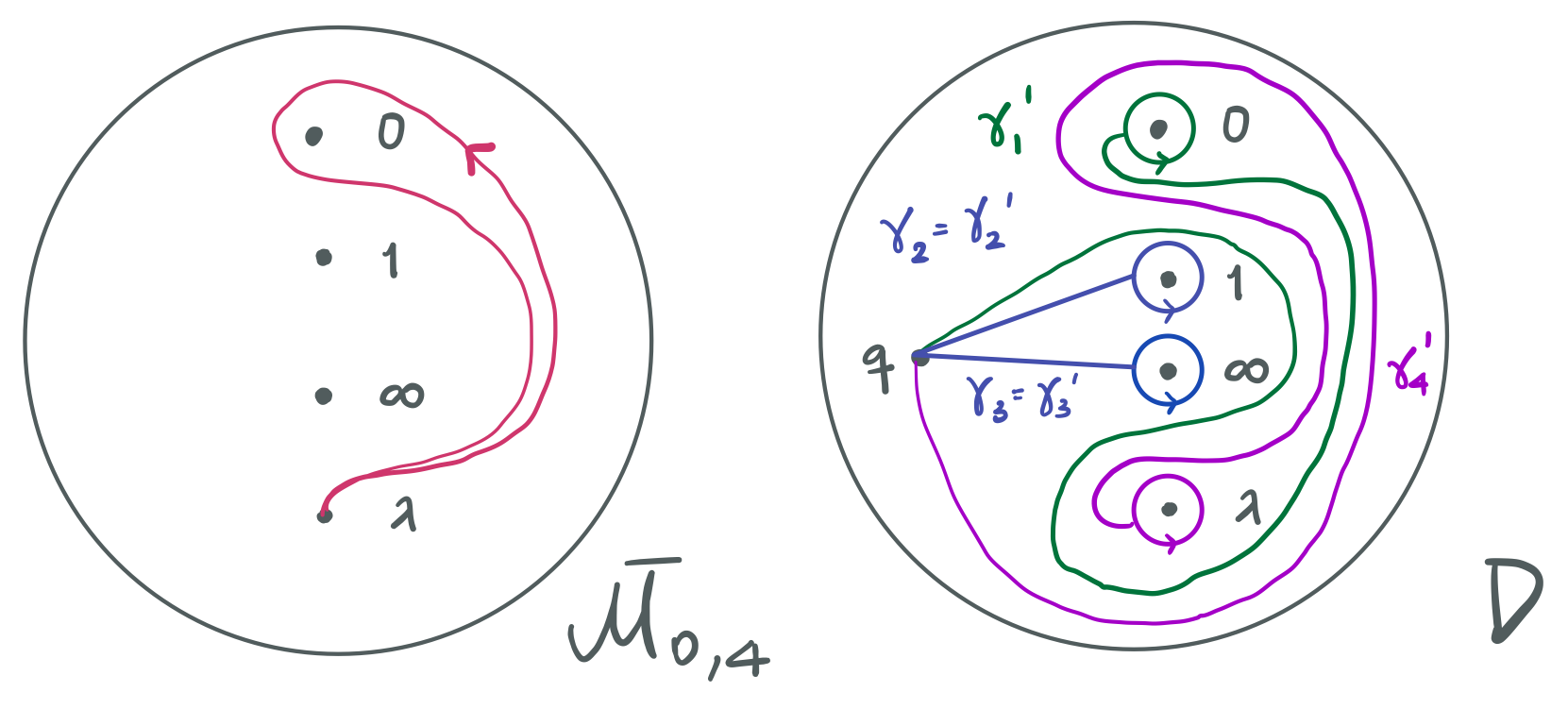
Finally, for a loop based at and winding once around (see Figure 7), the resulting monodromy representation with respect to the standard generating set is:
| (4) | ||||
5.3.3. Python program for computing monodromy of target map.
By calculating the endpoints of lifts of loops to , we can compute the monodromy of . We implemented this calculation in Python. The code (with examples) for this program is provided at https://github.com/amyqhli/1dim-hurwitz-space-monodromy-calculator. We briefly describe the algorithm here.
Given a Hurwitz space , we first set degree equal to and produce a list of tuples candidates where has ramification profile . Second, we multiply (the order of multiplication matters) to check if each tuple of permutations multiplies to the identity using the function CheckIdentity(degree, candidates). This function outputs a list called successes. We add all the possible markings to each monodromy representation in successes, and then filter out tuples which are simultaneous conjugates of other tuples using the function marked_sc_eqclass(degree, marked_successes). We are left with a list equivs of simultaneous conjugacy classes of fully-marked monodromy representations. We create a dictionary HurwSpace which enumerates each tuple in equivs as "Sheet{i}" to keep track of the sheets in this Hurwitz space.
Next, for each tuple in this list, we apply the monodromy formulae in Equations 2, 3 and 4 and check its simultaneous conjugacy class using the function sheet_connections_with_markings(degree, HurwSpace). This data corresponds to sheets in the Hurwitz space coming together over and in (we call such sheets “connected by an edge”). We keep track of this information in a dictionary called combined_edges. Using this dictionary, we can calculate the connected components of the Hurwitz space via find_connected_components which searches for sheets connected to each other by an edge in combined_edges. We make a dictionary component_groups of the components and the sheets in each component. For each component in component_groups, the function ram_of_target_map calculates the degree and ramification of the target map over in . Finally, we output the genus of the Hurwitz space using the Riemann-Hurwitz formula. The permutations associated to the ramification of the target map are also provided.
6. Calculations of for
Here, we record the genus and degree of the target map on the components of for , calculated via the program described in Section 5.3.3. For , all the base cases have genus 0, proving Theorem 1.1. As is a finite group quotient of when the source curve is connected and all , this proves that and recovers the fact that .
In degree 4, we have three base cases with positive genus, which we list in Section 6.3. This implies that is nonvanishing when . In Section 6.4, we include an example of a postive genus Hurwitz space in degree 5.
In the notation for the Hurwitz spaces, exponential notation indicates repeated ramification profiles. For example, the ramification profiles is denoted .
6.1. Degree-2 admissible covers
| Space | # components of genus 0 and degree of the target map | |
|---|---|---|
| 1 | 1 w/ deg 1 | |
| 2 | 1 w/ deg 2 | |
| 3 | 8 w/ deg 1 |
6.2. Degree-3 admissible covers
| Space | # components of genus 0 and degree of the target map | |
|---|---|---|
| 1 | 3 w/ deg 1 | |
| 2 | 2 w/ deg 1 | |
| 3 | 1 w/ deg 2 | |
| 4 | 4 w/ deg 3 | |
| 5 | 1 w/ deg 6 | |
| 6 | 1 w/ deg 4 | |
| 7 | 1 w/ deg 1 | |
| 8 | 9 w/ deg 2 | |
| 9 | 216 w/ deg 1 |
6.3. Degree-4 admissible covers.
| Space | # components of genus 0 with degree of the target map | |
|---|---|---|
| 1 | 4 w/ deg 1, 1 w/ deg 4 | |
| 2 | 3 w/ deg 2 | |
| 3 | 3 w/ deg 2 | |
| 4 | 6 w/ deg 1 | |
| 5 | 1 w/ deg 6 | |
| 6 | 2 w/ deg 4 | |
| 7 | 1 w/ deg 12 | |
| 8 | 2 w/ deg 4 | |
| 9 | 1 w/ deg 2, 1 w/ deg 6 | |
| 10 | 1 component of genus 3 mapping with degree 24 | |
| 11 | 2 w/ deg 8, 2 w/ deg 2 | |
| 12 | 36 w/ deg 4 | |
| 13 | 6 w/ deg 2 | |
| 14 | 2 w/ deg 8 | |
| 15 | 2 w/ deg 24 | |
| 16 | 2 w/ deg 16 | |
| 17 | 6 w/ deg 8 | |
| 18 | 3 w/ deg 2, 3 w/ deg 3 | |
| 19 | 12 w/ deg 4 | |
| 20 | 2 w/ deg 6 | |
| 21 | 2 w/ deg 4 | |
| 22 | 4 w/ degree 2 | |
| 23 | 2 w/ deg 8 | |
| 24 | 144 w/ deg 2 | |
| 25 | 1 component of genus 1, mapping with degree 24 | |
| 26 | 4 w/ deg 12 | |
| 27 | 12 w/ deg 4 | |
| 28 | 3 w/ deg 1 | |
| 29 | 2 components of genus 1, each mapping with degree 12 | |
| 30 | 8 w/ deg 1 | |
| 31 | 2 w/ deg 12 | |
| 32 | 4 w/ deg 2 | |
| 33 | 64 w/ deg 3 | |
| 34 | 16 w/ deg 6 | |
| 35 | 16 w/ deg 4 | |
| 36 | 6 w/ deg 2 | |
| 37 | 8 w/ deg 1 | |
| 38 | 288 w/ deg 2 | |
| 39 | 13824 w/ deg 1 |
6.4. Degree-5 admissible covers.
Example 6.1.
The Hurwitz space has 3 components of genus 0, 1 component of genus 1, and 1 component of genus 3.
References
- [ACV03] (2003) Twisted bundles and admissible covers. Comm. Algebra 31 (8), pp. 3547–3618. Note: Special issue in honor of Steven L. Kleiman External Links: ISSN 0092-7872,1532-4125, Document, Link, MathReview (Andrew Kresch) Cited by: §1, §2.1, §2.1.
- [AC98] (1998) Calculating cohomology groups of moduli spaces of curves via algebraic geometry. Publications Mathématiques de l’IHÉS 88, pp. 97–127. Cited by: §1, §1, §1, §5.1.
- [BFP24] (2024) Polynomial point counts and odd cohomology vanishing on moduli spaces of stable curves. Annals of Mathematics 199 (3), pp. 1323–1365. Cited by: §1.
- [CL22] (2022) Chow rings of low-degree Hurwitz spaces. Journal für die reine und angewandte Mathematik (Crelles Journal) 2022 (789), pp. 103–152. Cited by: §2.1.
- [CMR14] (2014-01) Tropicalizing the space of admissible covers. Mathematische Annalen 364, pp. . External Links: Document Cited by: §2.1, §4.
- [DP15] (2015) The Picard rank conjecture for the Hurwitz spaces of degree up to five. Algebra & Number Theory 9 (2), pp. 459 – 492. External Links: Document, Link Cited by: §1, §2.1.
- [DE96] (1996) Towards the homology of hurwitz spaces. Journal of Differential Geometry 43, pp. 66–98. External Links: Link Cited by: §1.
- [FP05] (2005) Relative maps and tautological classes. J. Eur. Math. Soc. 7 (1), pp. 13–49. External Links: ISBN , Document, Link Cited by: §2.1.
- [FUL69] (1969) Hurwitz schemes and irreducibility of moduli of algebraic curves. Annals of Mathematics 90 (3), pp. 542–575. External Links: ISSN 0003486X, 19398980, Link Cited by: §3.
- [HM06] (2006) Moduli of curves. Vol. 187, Springer Science & Business Media. Cited by: Remark 2.5.
- [HM82] (1982) On the Kodaira dimension of the moduli space of curves. Inventiones mathematicae. Cited by: §1, §2.1.
- [LL25] (2025) Homological stability for hurwitz spaces and applications. arXiv:2503.03861. Cited by: §1.
- [MUL23] (2023) The Hurwitz space Picard rank conjecture for . Adv. Math. 430, pp. Paper No. 109211, 27. External Links: ISSN 0001-8708,1090-2082, Document, Link, MathReview Entry Cited by: §1, §2.1.
- [Sv20] (2020) Intersections of loci of admissible covers with tautological classes. Selecta Math. (N.S.) 26 (5), pp. Paper No. 79, 69. External Links: ISSN 1022-1824,1420-9020, Document, Link, MathReview (Hülya Argüz) Cited by: §2.1.
- [ZHE22] (2022) Rational cohomology of the moduli space of trigonal curves of genus 5. manuscripta mathematica 169 (3), pp. 603–631. Cited by: §2.1.