A signature-based spatial scan statistic for functional data

Camille Frévent Corresponding author: camille.frevent@univ-lille.fr Univ. Lille, CHU Lille, ULR 2694 - METRICS: Évaluation des technologies de santé et des pratiques médicales, F-59000 Lille, France

Abstract

We have developed a new signature-based spatial scan statistic for functional data (SigFSS). This scan statistic can be applied to both univariate and multivariate functional data. In a simulation study, SigFSS almost always performed better than the literature approaches and yielded more precise clusters in geographic terms. Lastly, we used SigFSS to search for spatial clusters of abnormally high or abnormally low mortality rates in mainland France.
Keywords: Cluster detection, Functional data, Signature, Spatial scan statistics

1 Introduction

In many applications, researchers seek to determine the presence or absence of aggregations of spatial units (namely spatial clusters) that behave unusually. Various categories of spatial cluster detection tests have been developed. For example, non-focused cluster detection tests can usefully detect statistically significant spatial clusters without the a priori need for information about the latter’s location. Within this category, spatial scan statistics use a scanning window to detect statistically significant spatial clusters of various sizes and shapes without pre-selection bias.
Accordingly, spatial scan statistics have been applied to many fields of applied research, such as epidemiology (Costa-Nobre et al., 2024; Jiao et al., 2024; Wang et al., 2025), environmental sciences (Chong et al., 2013; Duncan et al., 2016), and criminology (Saravag and B, 2024; de Paula Alves and de Oliveira Batista, 2024).

These methods were initially introduced by Kulldorff and Nagarwalla (1995) and Kulldorff (1997) for Bernoulli and Poisson data distributions but have since been extended to many other spatial data distributions, such as Gaussian (Kulldorff et al., 2009), ordinal (Jung et al., 2007) and zero-inflated (Cançado et al., 2014; de Lima et al., 2015; Cançado et al., 2017) models. In the context of multivariate data, Kulldorff et al. (2007) developed a parametric approach based on the combination of independent univariate scan statistics. This method does not, however, take account of correlations between variables. This obstacle was circumvented by Cucala et al. (2017) and Cucala et al. (2019), who developed spatial scan statistics designed specifically for multivariate data by taking account of correlations between variables.

Thanks to advances in sensing technology and data storage capacities, data are increasingly being measured continuously over time. This prompted the introduction of functional data analysis by Ramsay and Silverman (1997) and the adaptation of classical statistical methods (such as clustering (Jacques and Preda, 2014; Zhang and Parnell, 2023), principal component analysis (PCA) (Boente and Fraiman, 2000; Berrendero et al., 2011) and regression (Cuevas et al., 2002; Ferraty and Vieu, 2002; Chiou and Müller, 2007)) to a functional framework.
In domains where data naturally involve a spatial component (e.g., demographics, environmental science, and agricultural science (Hung, 2016)), the emergence of functional data has led to the introduction of spatial functional data and the development of new methods for clustering (Giraldo et al., 2012; Vandewalle et al., 2021), kriging (Giraldo et al., 2011; Ignaccolo et al., 2014), PCA (Liu et al., 2017a; Si-Ahmed et al., 2025) or regression (Attouch et al., 2011; Bernardi et al., 2017).

In the field of spatial scan statistics, the detection of spatial clusters characterized by abnormal observed values of a stochastic process is an active research topic. Frévent et al. (2021) and Smida et al. (2022) first developed parametric and nonparametric approaches for the detection of spatial clusters on univariate functional data; the methods were based on an analysis of variance, Student’s t-test, and Wilcoxon-Mann-Whitney test statistics, respectively. Recently, Smida et al. (2025) developed a new approach based on a Hotelling test statistic. Furthermore, Frévent et al. (2023) developed three new approaches suited to use with a multivariate, functional data framework.

In recent years, signatures - initially defined by Chen (1957, 1977) for smooth paths and rediscovered in the context of rough path theory (Lyons, 1998; Friz and Victoir, 2010) - have been widely used in many domains, such as character recognition (Graham, 2013; Liu et al., 2017b; Xie et al., 2018), medicine (Perez Arribas et al., 2018; Morrill et al., 2020), and finance (Gyurkó et al., 2013; Arribas, 2018; Perez Arribas, 2020). Fermanian (2022) recently investigated their use in the context of a linear regression model with functional covariates. Frévent (2025) and Frévent and Dabo (2024) extended this approach to a spatial autoregressive model with functional covariates, in the context of an univariate outcome and a multivariate outcome, respectively.
For the analysis of functional data, signatures offer several advantages over classical approaches: they are (i) applicable to a wide range of processes that are not necessarily square-integrable, (ii) naturally suited to use with multivariate functions, and (iii) suitable for encoding a process’s geometric properties (Fermanian, 2022).

Here, we describe a new, signature-based spatial scan statistic for use with both univariate and multivariate functional data.
Section 2 serves as an introduction to the notion of signatures. Section 3 describes our new approach to the detection of spatial clusters in functional data. Section 4 presents both the design and the results of simulation studies in which our new approach was compared with existing methods in univariate and multivariate functional contexts. The results of application of our method to a real dataset are presented in Section 5. Lastly, our results are discussed in Section 6.

2 The concept of signatures

This section provides a brief introduction to the concept of signatures. For a more comprehensive description, we refer the reader to Lyons et al. (2007); Friz and Victoir (2010). It should be borne in mind that although signatures were initially formulated for smooth paths, we use them in the context of functional data and thus, for ease of understanding, employ the associated notations.

Let $X:\mathcal{T}\rightarrow\mathbb{R}^{p}$ be a $p$ -dimensional continuous function of bounded variation, that is

\left\|X\right\|_{TV}=\sup_{(t_{0},...,t_{k})\in\mathcal{I}}\sum_{i=1}^{k}\left\|X(t_{i})-X(t_{i-1})\right\|<+\infty,

where $\left\|.\right\|_{TV}$ denotes the total variation distance, $\left\|.\right\|$ denotes the Euclidean norm on $\mathbb{R}^{p}$ , and $\mathcal{I}$ denotes the set of all finite partitions of $\mathcal{T}$ .

Definition 1.

The signature of $X$ is defined by

Sig(X)=(1,\bm{X}^{1},\dots,\bm{X}^{d},\dots)

where

\bm{X}^{d}=\underset{\begin{subarray}{c}t_{1}<\dots<t_{d}\\ t_{1},\dots,t_{d}\in\mathcal{T}\end{subarray}}{\displaystyle\int\dots\displaystyle\int}\ \text{d}X(t_{1})\otimes\dots\otimes\text{d}X(t_{d})\in\left(\mathbb{R}^{p}\right)^{\otimes d}.

Definition 2.

The truncated signature of $X$ at order $D\geq 1$ is

Sig^{D}(X)=(1,\bm{X}^{1},\dots,\bm{X}^{D}).

Definition 3.

The truncated signature coefficient vector of $X$ at order $D$ is defined as

S^{D}(X)=\left(1,S_{(1)}(X),\dots,S_{(p)}(X),S_{(1,1)}(X),S_{(1,2)}(X),\dots,S_{\underbrace{\scriptstyle(p,\ldots,p)}_{\text{length }D}}(X)\right),

and the truncated shifted-signature coefficient vector of $X$ at order $D$ is defined as follows

\widetilde{S}^{D}(X)=\left(S_{(1)}(X),\dots,S_{(p)}(X),S_{(1,1)}(X),S_{(1,2)}(X),\dots,S_{\underbrace{\scriptstyle(p,\ldots,p)}_{\text{length }D}}(X)\right),

where for all $d\geq 1$ and for all multi-index , $(i_{1},\dots,i_{d})\subset\{1,\dots,p\}^{d}$ ,

S_{(i_{1},\dots,i_{d})}(X)=\underset{\begin{subarray}{c}t_{1}<\dots<t_{d}\\ t_{1},\dots,t_{d}\in\mathcal{T}\end{subarray}}{\displaystyle\int\dots\displaystyle\int}\ \text{d}X^{(i_{1})}(t_{1})\dots\text{d}X^{(i_{d})}(t_{d})\in\mathbb{R}.

Next, the truncated shifted-signature coefficient vector of $X$ at order $D$ is a vector of length

\widetilde{s}_{p}(D)=\sum_{d=1}^{D}p^{d}=\frac{p^{D+1}-p}{p-1}\text{ if }p\geq 2\text{ and }\widetilde{s}_{p}(D)=D\text{ if }p=1.

Lemma 1.

Let $\Psi:\mathcal{T}\rightarrow\mathcal{T}$ be a non-decreasing surjection and

	$\displaystyle Y:\mathcal{T}$	$\displaystyle\longrightarrow\mathbb{R}^{p}$
	$\displaystyle t$	$\displaystyle\longmapsto X({\Psi(t)}).$

Next, $Sig(X)=Sig(Y)$ : the signature of $X$ is invariant by time reparameterization.

Lemma 2.

Let

	$\displaystyle Y:\mathcal{T}$	$\displaystyle\longrightarrow\mathbb{R}^{p}$
	$\displaystyle t$	$\displaystyle\longmapsto X(t)+a,a\neq 0.$

Next, $Sig(X)=Sig(Y)$ : the signature of $X$ is invariant by translation.

Lemma 3.

It is possible to (i) circumvent the invariance by translation by adding an observation point taking the value 0 at the beginning of $X$ , and (ii) avoid the invariance by time reparameterization by considering the time-augmented function

	$\displaystyle\widetilde{X}:\mathcal{T}$	$\displaystyle\longrightarrow\mathbb{R}^{p+1}$
	$\displaystyle t$	$\displaystyle\longmapsto\left(X(t)^{\top},t\right)^{\top}$

instead of $X$ .

3 Methodology

3.1 General principle

Let $X:\mathcal{T}\rightarrow\mathbb{R}^{p}$ be a $p$ -dimensional continuous stochastic process of bounded variation and $s_{1},\dots,s_{n}$ be $n$ non-overlapping spatial locations of an observation domain $\mathcal{S}\subset\mathbb{R}^{2}$ . Let $X_{1},\dots,X_{n}$ be the observations of $X$ in $s_{1},\dots,s_{n}$ . Hereafter, all observations are considered to be independent; this is a classical assumption in scan statistics.

Spatial scan statistics are designed to detect spatial clusters and then test the latter’s statistical significance. Hence, one tests a null hypothesis $\mathcal{H}_{0}$ (the absence of a cluster) against a composite alternative hypothesis $\mathcal{H}_{1}$ (the presence of at least one spatial cluster $w\subset\mathcal{S}$ presenting abnormal values of $X$ , compared with the rest of the domain).

According to Cressie (1977), a scan statistic is the maximum of a concentration index over a set of potential clusters $\mathcal{W}$ . In the following and without loss of generality, we focus on the variable-size circular clusters introduced by Kulldorff (1997). The set of potential circular clusters $\mathcal{W}$ is defined by the following set of discs $w_{i,j}$ centered on $s_{i}$ and passing through $s_{j}$ :

\mathcal{W}=\{w_{i,j}/1\leq|w_{i,j}|\leq n,1\leq i,j\leq n\},

where $|w_{i,j}|$ is the number of sites in $w_{i,j}$ . Thus, as recommended by Kulldorff and Nagarwalla (1995), a cluster cannot cover more than 50% of the studied region.

3.2 The signature-based spatial scan statistic for functional data

3.2.1 Computation of the signatures

In the signature-based spatial scan statistic for functional data (SigFSS), we first calculated the truncated signature of $X$ in each spatial location. The objective is to detect the spatial clusters in which the distribution of $X$ is abnormal; temporal concordance is important but the height of the curves (relative to the others) is also important. Thus, invariance by translation and by time reparameterization are not desirable, and we used the strategy described in Lemma 3 to avoid them.

Furthermore, in order to encode the maximum amount of available information on $X_{1},\dots,X_{n}$ , the truncation order is important. Here and in the following, we shall set a truncation order $D$ such that $\widetilde{s}_{p+1}(D)$ is at most $10^{4}$ , similar to Frévent (2025).

At the end of this step, the dataset consisted of $\widetilde{S}^{D}(\widetilde{X}_{1}),\dots,\widetilde{S}^{D}(\widetilde{X}_{n})$ where $\widetilde{X}_{i}$ is defined as

	$\displaystyle\widetilde{X}_{i}:\mathcal{T}$	$\displaystyle\longrightarrow\mathbb{R}^{p+1}$
	$\displaystyle t$	$\displaystyle\longmapsto\left(X_{i}(t)^{\top},t\right)^{\top},$

after adding the value 0 at the beginning of $X_{i}$ .

3.2.2 Reduction of dimension

Encoding the functions $X_{1},\dots,X_{n}$ with truncated signatures transformed them into vectors of size $\widetilde{s}_{p+1}(D)\leq 10^{4}$ . This value is generally very large and greater than $n$ . Hence, it is therefore mathematically impossible to apply spatial scan statistics to the vectors without reducing their dimension.

Thus, the second step in the SigFSS approach was to reduce the dimension of $\widetilde{S}^{D}(\widetilde{X}_{1}),\dots,\widetilde{S}^{D}(\widetilde{X}_{n})$ using a PCA.

The data $\widetilde{S}^{D}(\widetilde{X}_{1}),\dots,\widetilde{S}^{D}(\widetilde{X}_{n})$ is thus transformed to $\zeta_{1}^{(D,K)},\dots,\zeta_{n}^{(D,K)}$ where

\zeta_{i}^{(D,K)}=\left(\zeta_{i,1}^{(D)},\dots,\zeta_{i,K}^{(D)}\right)^{\top}

is the vector of the $K$ first scores computed for $\widetilde{S}^{D}(\widetilde{X}_{i})$ on the $K$ first axes.

The number $K$ of principal components was chosen as a function of the cumulative inertia criterion. Two approaches can be considered: $K$ is determined such that the cumulative inertia (i) reaches a fixed threshold (95%, for example, as considered in Ahmed and Genin (2020)), or (ii) shows a marginal increase towards 1 (Smida et al., 2025).

3.2.3 Computing the spatial scan statistic

Once the size of the signatures has been reduced through the use of principal scores, we consider the following test hypotheses:

$\mathcal{H}_{0}$ : $\zeta_{1}^{(D,K)},\dots,\zeta_{n}^{(D,K)}$ are identically distributed, whatever their associated locations $s_{1},\dots,s_{n}$

vs.

$\mathcal{H}_{1}$ : There exists $w\in\mathcal{W}$ such that the distribution of $\zeta^{(D,K)}$ in $w$ differs from that of $\zeta^{(D,K)}$ outside $w$ .

In the context of multivariate data, Cucala et al. (2019) developed a nonparametric spatial scan statistic that relies on the extension of the Wilcoxon-Mann-Whitney test statistic for multivariate data, as defined by Oja and Randles (2004).

Let $\text{sgn}_{K}(\cdot)$ be the multivariate sign function defined as

\begin{array}[]{rccl}\text{sgn}_{K}:&\mathbb{R}^{K}&\rightarrow&\mathbb{R}^{K}\\ &z&\mapsto&||z||_{2}^{-1}z\ \mathds{1}_{z\neq\bm{0}_{K}}\end{array}

with $\bm{0}_{K}$ the $K$ -dimensional vector composed only of 0, and let

R_{i}=\dfrac{1}{n}\displaystyle\sum_{j=1}^{n}\text{sgn}_{K}\left[A_{\zeta^{(D,K)}}\left(\zeta_{i}^{(D,K)}-\zeta_{j}^{(D,K)}\right)\right]

be the multivariate ranks, where $A_{\zeta^{(D,K)}}$ is a data-based transformation matrix that makes the multivariate ranks behave as though they were spherically distributed in the unit $K$ -sphere:

\dfrac{K}{n}\displaystyle\sum_{i=1}^{n}R_{i}R_{i}^{\top}=\dfrac{1}{n}\displaystyle\sum_{i=1}^{n}R_{i}^{\top}R_{i}I_{K}.

To test

$\mathcal{H}_{0}:$ The distribution of $\zeta^{(D,K)}$ is the same inside and outside $w$

vs.

$\mathcal{H}_{1}:$ The distribution of $\zeta^{(D,K)}$ in $w$ differs from that of $\bm{Z}$ outside $w$ ,

we can consider the following test statistic developed by Oja and Randles (2004):

W^{(w)}=\dfrac{Kn}{\displaystyle\sum_{i=1}^{n}R_{i}^{\top}}\left(|w|||\bar{R}_{w}||_{2}^{2}+|w^{\mathsf{c}}|||\bar{R}_{w^{\mathsf{c}}}||_{2}^{2}\right)

where $\bar{R}_{g}=\dfrac{1}{|g|}\displaystyle\sum_{\begin{subarray}{c}i=1\\ s_{i}\in g\end{subarray}}^{n}R_{i},g\in\{w,w^{\mathsf{c}}\}$ .

Next, in the same way as Cucala et al. (2019), we considered $W^{(w)}$ to be a concentration index for cluster detection and we defined the SigFSS statistic as

\lambda_{\text{SigFSS}}=\underset{w\in\mathcal{W}}{\max}\ W^{(w)}.

The most likely cluster (MLC) was the potential cluster for which this maximum is obtained:

\text{MLC}_{\text{SigFSS}}=\underset{w\in\mathcal{W}}{\arg\max}\ W^{(w)}.

3.2.4 Statistical significance

Once the MLC has been identified, its statistical significance must be evaluated. The distribution of the scan statistic is intractable under $\mathcal{H}_{0}$ , due to the overlap between the two concentration indices $W^{(w)}$ and $W^{(w^{\prime})}$ when $w\cap w^{\prime}\neq\emptyset$ .

Thus, we employed an approach based on random permutations (commonly referred to as “random labelling”) to estimate the p-value associated with $\lambda_{\text{SigFSS}}$ .

Let $P$ denote the number of random permutations performed on the original dataset, and $\lambda_{\text{SigFSS}}^{(1)},\dots,\lambda_{\text{SigFSS}}^{(P)}$ denote the spatial scan statistics obtained from these permuted datasets. According to Dwass (1957), the p-value for the scan statistic observed in the original data can be estimated as follows:

\widehat{p}=\dfrac{1+\displaystyle\sum_{p^{\prime}=1}^{P}\mathds{1}_{\lambda_{\text{SigFSS}}^{(p^{\prime})}\geq\lambda_{\text{SigFSS}}}}{1+P}.

The MLC was considered to be statistically significant when its associated estimated p-value was smaller than the type I error.

3.2.5 Secondary clusters

In practice, it is sometimes necessary to detect secondary clusters. Here, we considered the approach of Kulldorff (1997), which defines secondary clusters as geographical areas corresponding to a second maximum of the concentration index, then a third maximum, and so on. The p-value of the secondary clusters is calculated by comparing the values of their associated concentration index with the value of $\lambda_{\text{SigFSS}}^{(p^{\prime})}$ . It should be noted that this approach is rather conservative because for a secondary cluster to be declared statistically significant, it must be able to reject $\mathcal{H}_{0}$ per se, as if it were the MLC itself. Lastly, only statistically significant secondary clusters that did not overlap with a more likely cluster were considered.

4 The simulation study

In a simulation study, we compared the new SigFSS with the DFFSS, the PFSS (Frévent et al., 2021), the URBFSS (Frévent et al., 2022), the NPFSS (Smida et al., 2022) and the HFSS (Smida et al., 2025) in the univariate case and with the MDFFSS, the MPFSS, the MRBFSS (Frévent et al., 2023) and the NPFSS (Smida et al., 2022) in the multivariate case.

4.1 Design of the simulation study

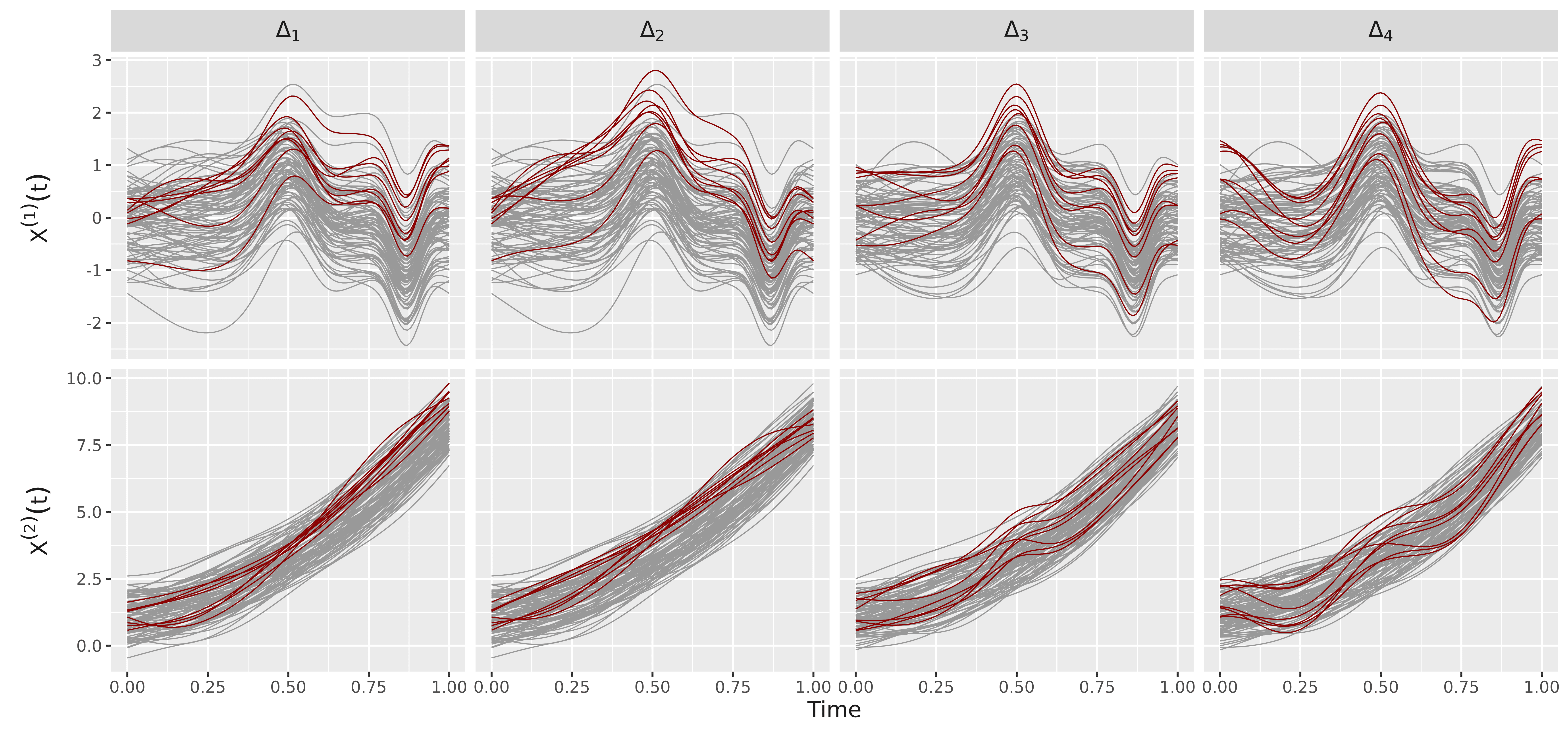
Artificial datasets were generated for the geographical locations of the 94 départements (administrative counties) in mainland France (see Figure S1 in the Supplementary Materials). The location of each département was defined by its centroid. For each artificial dataset, a spatial cluster $w$ composed of eight départements in the Paris region was simulated (the area highlighted in red in Figure S1 in Supplementary Materials).

We considered the cases $p=1$ and $p=2$ . The $X_{i}$ were simulated according to the following model considered in Frévent et al. (2023), and were measured at 101 equally spaced times on $[0,1]$ :

X_{i}(t)=\mu+\Delta(t)\mathds{1}_{s_{i}\in w}+\varepsilon_{i}(t),\ t\in[0,1],

where $\mu=\sin{(2\pi t^{2})}^{5}$ if $p=1$ and $\mu=(\sin{(2\pi t^{2})}^{5},1+2.3t+3.4t^{2}+1.5t^{3})^{\top}$ if $p=2$ , $\varepsilon_{i}(t)=\displaystyle\sum_{k=1}^{100}Z_{i,k}\sqrt{1.5\times 0.2^{k}}\theta_{k}(t)$ , with $\theta_{k}(t)=\left\{\begin{array}[]{ll}1&\text{ if }k=1\\ \sqrt{2}\sin{[k\pi t]}&\text{ if }k\text{ even}\\ \sqrt{2}\cos{[(k-1)\pi t]}&\text{ if }k\text{ odd and }k>1\end{array}\right.$ .

By denoting $\Sigma=\begin{pmatrix}1&\rho\\ \rho&1\end{pmatrix}$ the covariance matrix of the $Z_{i,k}$ when $p=2$ , and considering $\Sigma=1$ when $p=1$ , three distributions of the $Z_{i,k}$ were used: (i) a normal distribution: $Z_{i,k}\sim\mathcal{N}(0,\Sigma)$ , (ii) a standardized Student distribution: $Z_{i,k}=U_{i,k}\left(\dfrac{V_{i,4}}{4}\right)^{-0.5}$ where the $U_{i,k}$ are independent $\mathcal{N}(0,\Sigma/2)$ variables and the $V_{i,4}$ are independent $\chi_{2}(4)$ variables, and (iii) a standardized exponential distribution: $Z_{i,k}=\left[U_{i,k}-\begin{pmatrix}2\\ 2\end{pmatrix}\right]/2$ where the $U_{i,k}$ are independent and $U_{i,k}\sim\mathcal{E}(\frac{1}{2},\Sigma)$ .

Three values of $\rho$ ( $\rho=0.2,0.5,0.8$ ) were tested for $p=2$ , and four types of clusters (whose intensity was controlled by a parameter $\alpha>0$ ) were studied: $\Delta_{1}(t)=\alpha(t,t)^{\top}$ , $\Delta_{2}(t)=\alpha(t(1-t),t(1-t))^{\top}$ , $\Delta_{3}(t)=\alpha(\exp{(-100(t-0.5)^{2})}/3,\exp{(-100(t-0.5)^{2})}/3)^{\top}$ , and $\Delta_{4}(t)=\alpha(\cos{(4\pi(t-0.5))},\cos{(4\pi(t-0.5))})^{\top}$ , together with the respective univariate versions when $p=1$ .

Different values of the parameter $\alpha$ were considered for each $\Delta$ : $\alpha\in\{0,0.25,0.5,0.75,1\}$ for $\Delta_{1}$ , $\alpha\in\{0,1,2,3,4\}$ for $\Delta_{2}$ , $\alpha\in\{0,0.5,1,1.5,2\}$ for $\Delta_{3}$ , $\alpha\in\{0,0.125,0.25,0.375,0.5\}$ for $\Delta_{4}$ .

Note that $\alpha=0$ was also tested, in order to evaluate the conservation of the nominal type I error. An example of the data for $p=1$ and for $p=2$ with $\rho=0.2$ (when considering a Gaussian distribution for the $Z_{i,k}$ ) is given in Supplementary Materials (Figures S2 and S3).

4.2 Comparison of the methods

In both the univariate and multivariate cases, and for each $Z_{i,k}$ distribution, we simulated each $\Delta$ , each $\rho$ (in the multivariate case), and each value of $\alpha$ in 200 artificial datasets. A total of 999 samples were generated by random permutations of the data, and the type I error was set to 0.05. The methods’ respective performance levels were compared with regard to four criteria: the power, the true positive rate, the false positive rate, and the positive predictive value.

The power was estimated as the proportion of simulations leading to the rejection of $\mathcal{H}_{0}$ , depending on the type I error. Among the simulated datasets leading to the rejection of $\mathcal{H}_{0}$ , the true positive rate is the mean proportion of sites correctly detected among the sites in $w$ , the false positive rate is the mean proportion of sites in $w^{\mathsf{c}}$ that were included in the detected cluster, and the positive predictive value corresponds to the mean proportion of sites in $w$ within the detected cluster.

For the SigFSS and the HFSS, we also compared the performance levels by choosing a value of $K$ such that the cumulative inertia showed a marginal increase towards 1 (graphic approach) or reached a fixed threshold of 95% or 99%.

4.3 Results of the simulation study

The results of the simulation are presented in Figures 1, 2, 3 and 4 for when $K$ was chosen graphically (see also Figures S4, S5 and S8 in the Supplementary Materials), in Figures S6, S9, S10, S11 for when a fixed threshold of 95% for the cumulative inertia was applied, and in Figures S7, S12, S13, S14 in the Supplementary Materials for when a fixed threshold of 99% was applied.

For $\alpha=0$ , all methods yielded a type I error of 0.05, regardless of the type of process, the type of $\Delta$ , and the level of correlation $\rho$ (for the multivariate processes).

In the univariate case, when $K$ is chosen graphically and $\Delta=\Delta_{1}$ , the SigFSS yielded the highest power, true positive rate and positive predictive value and the lowest false positive rate. When $\Delta=\Delta_{2}$ and $\Delta=\Delta_{3}$ , the SigFSS presented the lowest false positive rate and the highest positive predictive value. It also presented a high true positive rate and the greatest power when considering a non-Gaussian process. When $\Delta=\Delta_{4}$ , the power of the SigFSS was higher than those of the PFSS, NPFSS, DFFSS and URBFSS but lower than that of the HFSS. However, the false positive rates and the positive predictive values were similar.

When considering a fixed threshold of 95% or 99% for the cumulative inertia, the SigFSS always presented the highest power, true positive rate and positive predictive value and the lowest false positive rate.

When considering a multivariate process ( $p=2$ ), regardless of whether $K$ is chosen graphically or according to a fixed threshold of 95% or 99% for the cumulative inertia and regardless of the value of $\rho$ , the SigFSS always performed best with regard to the power, true positive rate, false positive rate, and positive predictive value.

Refer to caption — Figure 1: The simulation study (univariate case): a comparison of the SigFSS, HFSS, NPFSS, DFFSS, URBFSS, and PFSS methods for detection of the spatial cluster as the MLC, when considering a graphical approach for choosing $K$ in the SigFSS and the HFSS. $\alpha$ is the parameter that controls the cluster intensity.

5 Application to real data

5.1 The mortality rate in France

We considered data provided by the Institut National de la Statistique et des Etudes Economiques (Paris, France) on the annual mortality rate in each of the 94 French départements between 1979 and 2012. The all-cause mortality rate was used for the univariate case, and the mortality rate due to circulatory system diseases (CSDs) and respiratory diseases (RDs) was used for the multivariate case (Figures 5 and 6).

5.2 Spatial cluster detection

We used the DFFSS, the PFSS, the NPFSS, the URBFSS, the HFSS and the SigFSS to detect spatial clusters of low or elevated mortality rate. For the multivariate case, we used the MDFFSS, the MPFSS, the NPFSS, the MRBFSS and the SigFSS to detect atypical areas with regard to the mortality rate for CSDs or RDs.
For the HFSS and the SigFSS we considered a graphical approach for the choice of $K$ (see Figure S15 in Supplementary Materials) but we also considered fixed thresholds of 95% and 99% for the cumulative inertia (see Figures S16 and S17 and Tables S1 and S2 in Supplementary Materials).

For all methods, we considered the set of potential circular clusters $\mathcal{W}$ defined in Section 3. The statistical significance of the MLC or the secondary clusters was evaluated in 999 Monte-Carlo permutations. A spatial cluster was considered to be statistically significant when the associated p-value was below 0.05.

5.3 Results for the univariate case

All the methods detected two statistically significant spatial clusters (see Figure 7 and Table 1). One corresponded to a spatial aggregation of lower mortality rates and comprised départements from the Île-de-France region; depending on the method, some other départements were added to those in the Île-de-France. The other statistically significant spatial cluster was characterized by an elevated mortality rate relative to the rest of the study area and covered a large number of départements in southwestern France.

It is noteworthy that the SigFSS method yielded more precise (i.e., smaller) clusters.

When considering a threshold of 95% or 99% for the cumulative inertia, the clusters detected with the HFSS and the SigFSS were fairly similar.

Table 1: Statistically significant spatial clusters with a higher or lower mortality rate.

Method	Cluster	Number of départements	p-value
DFFSS	Most likely cluster	37	0.001
	Secondary cluster	9	0.001
PFSS	Most likely cluster	31	0.001
	Secondary cluster	9	0.001
NPFSS	Most likely cluster	31	0.001
	Secondary cluster	23	0.001
URBFSS	Most likely cluster	32	0.001
	Secondary cluster	23	0.001
HFSS	Most likely cluster	30	0.001
	Secondary cluster	7	0.002
SigFSS	Most likely cluster	4	0.001
	Secondary cluster	23	0.002

5.4 Spatial clusters detection in the multivariate case

As in the univariate case, all the methods detected two statistically significant spatial clusters in the multivariate case (see Figure 8 and Table 2). Furthermore, the clusters detected in the multivariate case were very similar to those detected in the univariate case. One cluster was located around the Île-de-France region and was associated with a lower CSD and RD mortality rate, compared with the rest of the spatial region. The other cluster was located in southwestern France and was associated with higher CSD and RD mortality rate than elsewhere.

Once again, the SigFSS method detected more precise clusters than the literature methods did. The SigFSS results were notably stable; there were few differences between the detected clusters when considering cumulative inertia thresholds of 95% or 99%.

Table 2: Statistically significant spatial clusters with an abnormal mortality rate due to circulatory system diseases and respiratory diseases.

Method	Cluster	Number of départements	p-value
MDFFSS	Most likely cluster	31	0.001
	Secondary cluster	13	0.026
MPFSS, NPFSS,	Most likely cluster	31	0.001
MRBFSS	Secondary cluster	23	0.001
SigFSS	Most likely cluster	9	0.001
	Secondary cluster	25	0.005

6 Discussion

We developed a SigFSS to detect spatial clusters in functional data. The method is based on signatures and presents the advantage of being applicable to both univariate and multivariate functional data.

In a simulation study of a univariate case, we compared the SigFSS with the PFSS (Frévent et al., 2021), the DFFSS (Frévent et al., 2021), the URBFSS (Frévent et al., 2022), the NPFSS (Smida et al., 2022) and the HFSS (Smida et al., 2025). We found that the SigFSS (i) almost always yielded the greatest power and the highest true positive rate (ii) always yielded the lowest false positive rate and the highest positive predictive value; this resulted in more precise clusters.

In a simulation study of a multivariate case, we compared the SigFSS with the MPFSS, the MDFFSS, the MRBFSS (Frévent et al., 2023) and the NPFSS (Smida et al., 2022). Again, the results showed that the SigFSS always outperformed the literature methods.

Next, we used the methods to detect spatial clusters of abnormal mortality rate in France. Two statistically significant clusters were detected by all methods: one near the Île-de-France region (characterized by a lower mortality rate, compared with the rest of France) and one in southwestern France (characterized by higher mortality rate). However, the clusters detected with the SigFSS were smaller, which was consistent with the results of the simulation study.

We also applied the methods to a multivariate functional dataset corresponding to the mortality rate due to CSDs and RDs; as in the univariate case, the methods detected two similar statistically significant clusters. One cluster was located near the Île-de-France region and was characterized by a lower mortality rate due to CSDs and RDs (compared with the rest of France), and the other was located in southwestern France and was characterized by a higher mortality rate due to CSDs and RDs. The clusters detected with the SigFSS were smaller than those detected by the MPFSS, the NPFSS, the MRBFSS and the MDFFSS.

It should be noted that we considered circular spatial clusters only. In fact, other cluster shapes might be relevant. For instance, Tango and Takahashi (2005) considered arbitrarily shaped clusters with a predefined maximum size by considering all sets of connected sites. However, it is important to note that this approach generates a significantly larger number of potential clusters (thereby involving greater computational time) than the method developed by Kulldorff (1997). The elliptical cluster approach developed by Kulldorff et al. (2006) is also associated with greater computational time. Lin et al. (2016) developed a potential alternative by suggesting the aggregation of circular clusters to form larger clusters of arbitrary shapes.

In practice, the detection of secondary clusters is often relevant. Here, we followed the approach developed by Kulldorff (1997), in which statistical inference is performed on other potential clusters as it is for the MLC. Zhang et al. (2010) suggests an alternative, sequential approach: once a statistically significant MLC has been detected, data are removed from the MLC (as if there were no spatial units there) and the MLC in the remaining data is then determined. If it is statistically significant, it is considered to be a secondary cluster. This approach is repeated until none of the clusters is statistically significant. A key limitation of these approaches is their failure to maintain the nominal type I error. The reliable inference of secondary clusters is challenging and requires further research.

It is noteworthy that in both the simulation study and the application to real data, the observation times were identical for all the spatial locations. While this represents an ideal scenario for functional data analysis, it is often not representative of real-world datasets. Nevertheless, our new method is applicable to spatial sites with different observation times because the signatures at each of the locations are computed independently.

The spatial scan statistic models presented here rely on the assumption whereby observations at different spatial locations are independent. This is a classical but strong assumption in the field of spatial scan statistics and is frequently violated in real-world applications - particularly in environmental datasets such as pollution measurements, where spatially close locations tend to exhibit similar values. The presence of spatial autocorrelation is known to lead to an inflation of the type I error in the random permutation procedure (Loh and Zhu, 2007; Lin, 2014; Lee et al., 2020; Ahmed et al., 2021). Although several recent works have explored the incorporation of spatial dependence into scan statistics (Lee et al., 2020; Ahmed et al., 2021), they focused on relatively simple models. The development of a method that account for spatial dependence within functional spatial scan statistics remains a challenge.

References

M. Ahmed, L. Cucala, and M. Genin (2021) Spatial autoregressive models for scan statistic. Journal of Spatial Econometrics 2 (1), pp. 11. Cited by: §6.
M. Ahmed and M. Genin (2020) A functional-model-adjusted spatial scan statistic. Statistics in medicine 39 (8), pp. 1025–1040. Cited by: §3.2.2.
I. P. Arribas (2018) Derivatives pricing using signature payoffs. arXiv preprint arXiv:1809.09466. Cited by: §1.
M. K. Attouch, A. Gheriballah, and A. Laksaci (2011) Robust nonparametric estimation for functional spatial regression. In Recent Advances in Functional Data Analysis and Related Topics, pp. 27–31. Cited by: §1.
M. S. Bernardi, L. M. Sangalli, G. Mazza, and J. O. Ramsay (2017) A penalized regression model for spatial functional data with application to the analysis of the production of waste in Venice province. Stochastic environmental research and risk assessment 31 (1), pp. 23–38. Cited by: §1.
J. R. Berrendero, A. Justel, and M. Svarc (2011) Principal components for multivariate functional data. Computational Statistics & Data Analysis 55 (9), pp. 2619–2634. Cited by: §1.
G. Boente and R. Fraiman (2000) Kernel-based functional principal components. Statistics & Probability Letters 48, pp. 335–345. External Links: Document Cited by: §1.
A. L. Cançado, C. Q. da-Silva, and M. F. da Silva (2014) A spatial scan statistic for zero-inflated Poisson process. Environmental and ecological statistics 21 (4), pp. 627–650. External Links: Document Cited by: §1.
A. L. Cançado, L. B. Fernandes, and C. Q. da-Silva (2017) A bayesian spatial scan statistic for zero-inflated count data. Spatial Statistics 20, pp. 57–75. External Links: Document Cited by: §1.
K. Chen (1957) Integration of paths, geometric invariants and a generalized Baker-Hausdorff formula. Annals of Mathematics, pp. 163–178. Cited by: §1.
K. Chen (1977) Iterated path integrals. Bulletin of the American Mathematical Society 83 (5), pp. 831–879. Cited by: §1.
J. Chiou and H. Müller (2007) Diagnostics for functional regression via residual processes. Computational Statistics & Data Analysis 15, pp. 4849–4863. External Links: Document Cited by: §1.
S. Chong, M. Nelson, R. Byun, L. Harris, J. Eastwood, and B. Jalaludin (2013) Geospatial analyses to identify clusters of adverse antenatal factors for targeted interventions. International Journal of Health Geographics 12 (46). External Links: Document Cited by: §1.
D. T. Costa-Nobre, A. S. S. Marinonio, M. H. Miyoshi, A. Sanudo, K. C. N. Areco, M. D. Kawakami, R. d. C. X. Balda, T. Konstantyner, C. N. V. e Oliveira, P. Bandiera-Paiva, et al. (2024) Space scan statistics to identify clusters of neonatal mortality associated with bacterial sepsis. Epidemiology & Infection 152, pp. e169. Cited by: §1.
N. Cressie (1977) On some properties of the scan statistic on the circle and the line. Journal of Applied Probability 14, pp. 272–283. Cited by: §3.1.
L. Cucala, M. Genin, C. Lanier, and F. Occelli (2017) A multivariate gaussian scan statistic for spatial data. Spatial Statistics 21, pp. 66–74. External Links: Document Cited by: §1.
L. Cucala, M. Genin, F. Occelli, and J. Soula (2019) A multivariate nonparametric scan statistic for spatial data. Spatial statistics 29, pp. 1–14. Cited by: §1, §3.2.3, §3.2.3.
A. Cuevas, M. Febrero-Bande, and R. Fraiman (2002) Linear functional regression: the case of fixed design and functional response. Canadian Journal of Statistics 30, pp. 285–300. External Links: Document Cited by: §1.
M. S. de Lima, L. H. Duczmal, J. C. Neto, and L. P. Pinto (2015) Spatial scan statistics for models with overdispersion and inflated zeros. Statistica Sinica 25 (1), pp. 225–241. External Links: Document Cited by: §1.
H. J. de Paula Alves and B. D. de Oliveira Batista (2024) Application of spatiotemporal scan statistics in cases of intentional homicides in northern Brazil. Brazilian Journal of Biometrics 42 (4), pp. 329–338. Cited by: §1.
D. Duncan, M. Rienti, M. Kulldorff, J. Aldstadt, M. Castro, R. Frounfelker, J. Williams, G. Sorensen, R. Johnson, D. Hemenway, and D. Williams (2016) Local spatial clustering in youths’ use of tobacco, alcohol, and marijuana in Boston. The American journal of drug and alcohol abuse 42 (4), pp. 412–421. External Links: Document Cited by: §1.
M. Dwass (1957) Modified randomization tests for nonparametric hypotheses. Annals of Mathematical Statistics 28 (1), pp. 181–187. External Links: Document Cited by: §3.2.4.
A. Fermanian (2022) Functional linear regression with truncated signatures. Journal of Multivariate Analysis 192, pp. 105031. Cited by: §1.
F. Ferraty and P. Vieu (2002) Functional nonparametric model and application to spectrometric data. Computational Statistics 17, pp. 545–564. External Links: Document Cited by: §1.
C. Frévent, M. Ahmed, S. Dabo-Niang, and M. Genin (2023) Investigating spatial scan statistics for multivariate functional data. Journal of the Royal Statistical Society Series C: Applied Statistics 72 (2), pp. 450–475. Cited by: §1, §4.1, §4, §6.
C. Frévent, M. Ahmed, M. Marbac, and M. Genin (2021) Detecting spatial clusters in functional data: new scan statistic approaches. Spatial Statistics 46, pp. 100550. Cited by: §1, §4, §6.
C. Frévent, M. Ahmed, J. Soula, Z. Smida, L. Cucala, S. Dabo-Niang, and M. Genin (2022) The R package HDSpatialScan for the detection of clusters of multivariate and functional data using spatial scan statistics.. R Journal 14 (3). Cited by: §4, §6.
C. Frévent and I. Dabo (2024) A multivariate spatial regression model using signatures. arXiv preprint arXiv:2410.07899. Cited by: §1.
C. Frévent (2025) A signature-based functional spatial autoregressive model. Electronic Journal of Statistics 19 (2), pp. 4541–4574. Cited by: §1, §3.2.1.
P. K. Friz and N. B. Victoir (2010) Multidimensional stochastic processes as rough paths: theory and applications. Vol. 120, Cambridge University Press. Cited by: §1, §2.
R. Giraldo, P. Delicado, and J. Mateu (2011) Ordinary kriging for function-valued spatial data. Environmental and Ecological Statistics 18 (3), pp. 411–426. Cited by: §1.
R. Giraldo, P. Delicado, and J. Mateu (2012) Hierarchical clustering of spatially correlated functional data. Statistica Neerlandica 66 (4), pp. 403–421. Cited by: §1.
B. Graham (2013) Sparse arrays of signatures for online character recognition. arXiv preprint arXiv:1308.0371. Cited by: §1.
L. G. Gyurkó, T. Lyons, M. Kontkowski, and J. Field (2013) Extracting information from the signature of a financial data stream. arXiv preprint arXiv:1307.7244. Cited by: §1.
M. Hung (2016) Applications of spatial statistics. IntechOpen, Rijeka. External Links: Document Cited by: §1.
R. Ignaccolo, J. Mateu, and R. Giraldo (2014) Kriging with external drift for functional data for air quality monitoring. Stochastic environmental research and risk assessment 28 (5), pp. 1171–1186. Cited by: §1.
J. Jacques and C. Preda (2014) Functional data clustering: a survey. Advances in Data Analysis and Classification 8 (3), pp. 231–255. Cited by: §1.
L. Jiao, T. Shen, Y. Han, W. Liu, W. Liu, L. Dang, M. Wei, Y. Yang, J. Guo, M. Miao, et al. (2024) The spatial-temporal distribution of hepatitis B virus infection in China, 2006–2018. BMC Infectious Diseases 24 (1), pp. 811. Cited by: §1.
I. Jung, M. Kulldorff, and A. C. Klassen (2007) A spatial scan statistic for ordinal data. Statistics in medicine 26 (7), pp. 1594–1607. Cited by: §1.
M. Kulldorff, L. Huang, and K. Konty (2009) A scan statistic for continuous data based on the normal probability model. Int J Health Geogr 8 (58). External Links: Document Cited by: §1.
M. Kulldorff, L. Huang, L. Pickle, and L. Duczmal (2006) An elliptic spatial scan statistic. Statistics in medicine 25, pp. 3929–3943. External Links: Document Cited by: §6.
M. Kulldorff, F. Mostashari, L. Duczmal, W. Yih, K. Kleinman, and R. Platt (2007) Multivariate scan statistics for disease surveillance. Statistics in medicine 26, pp. 1824–1833. External Links: Document Cited by: §1.
M. Kulldorff and N. Nagarwalla (1995) Spatial disease clusters: detection and inference. Statistics in Medicine 14 (8), pp. 799–810. External Links: Document, https://onlinelibrary.wiley.com/doi/pdf/10.1002/sim.4780140809, Link Cited by: §1, §3.1.
M. Kulldorff (1997) A spatial scan statistic. Communications in Statistics - Theory and Methods 26, pp. 1481–1496. External Links: Document Cited by: §1, §3.1, §3.2.5, §6, §6.
J. Lee, Y. Sun, and H. H. Chang (2020) Spatial cluster detection of regression coefficients in a mixed-effects model. Environmetrics 31 (2), pp. e2578. Cited by: §6.
P. Lin, Y. Kung, and M. Clayton (2016) Spatial scan statistics for detection of multiple clusters with arbitrary shapes. Biometrics 72 (4), pp. 1226–1234. Cited by: §6.
P. Lin (2014) Generalized scan statistics for disease surveillance. Scandinavian Journal of Statistics 41 (3), pp. 791–808. Cited by: §6.
C. Liu, S. Ray, and G. Hooker (2017a) Functional principal component analysis of spatially correlated data. Statistics and Computing 27 (6), pp. 1639–1654. Cited by: §1.
M. Liu, L. Jin, and Z. Xie (2017b) PS-LSTM: capturing essential sequential online information with path signature and LSTM for writer identification. In 2017 14th IAPR International Conference on Document Analysis and Recognition (ICDAR), Vol. 1, pp. 664–669. Cited by: §1.
J. M. Loh and Z. Zhu (2007) Accounting for spatial correlation in the scan statistic. The Annals of Applied Statistics 1 (2), pp. 560 – 584. External Links: Document Cited by: §6.
T. J. Lyons, M. Caruana, and T. Lévy (2007) Differential equations driven by rough paths. Springer. Cited by: §2.
T. J. Lyons (1998) Differential equations driven by rough signals. Revista Matemática Iberoamericana 14 (2), pp. 215–310. Cited by: §1.
J. H. Morrill, A. Kormilitzin, A. J. Nevado-Holgado, S. Swaminathan, S. D. Howison, and T. J. Lyons (2020) Utilization of the signature method to identify the early onset of sepsis from multivariate physiological time series in critical care monitoring. Critical Care Medicine 48 (10), pp. e976–e981. Cited by: §1.
H. Oja and R. H. Randles (2004) Multivariate nonparametric tests. Cited by: §3.2.3, §3.2.3.
I. Perez Arribas, G. M. Goodwin, J. R. Geddes, T. Lyons, and K. E. Saunders (2018) A signature-based machine learning model for distinguishing bipolar disorder and borderline personality disorder. Translational psychiatry 8 (1), pp. 274. Cited by: §1.
I. Perez Arribas (2020) Signatures in machine learning and finance. Ph.D. Thesis, University of Oxford. Cited by: §1.
J. Ramsay and B. Silverman (1997) Functional data analysis. Springer Series in Statistics, Springer. Cited by: §1.
P. K. Saravag and R. K. B (2024) An application of scan statistics in identification and analysis of hotspot of crime against women in Rajasthan, India. Applied Spatial Analysis and Policy 17 (3), pp. 963–982. Cited by: §1.
I. Si-Ahmed, L. Hamdad, C. J. Agonkoui, Y. Kande, and S. Dabo-Niang (2025) Principal component analysis of multivariate spatial functional data. Big Data Research 39, pp. 100504. Cited by: §1.
Z. Smida, L. Cucala, A. Gannoun, and G. Durif (2022) A Wilcoxon-Mann-Whitney spatial scan statistic for functional data. Computational Statistics & Data Analysis 167, pp. 107378. Cited by: §1, §4, §6, §6.
Z. Smida, T. Laurent, and L. Cucala (2025) A Hotelling spatial scan statistic for functional data: application to economic and climate data. Spatial Statistics 66, pp. 100888. Cited by: §1, §3.2.2, §4, §6.
T. Tango and K. Takahashi (2005) A flexibly shaped spatial scan statistic for detecting clusters. International journal of health geographics 4 (1), pp. 11. Cited by: §6.
V. Vandewalle, C. Preda, and S. Dabo-Niang (2021) Clustering spatial functional data. In Geostatistical Functional Data Analysis, pp. 155–174. Cited by: §1.
L. Wang, Y. Li, J. Chen, D. Zhang, Z. Zhang, and X. Li (2025) Spatiotemporal distribution and detection of spatial clusters of tuberculosis in Hubei province, China using FleXScan (2017–2023). BMC Public Health 25 (1), pp. 2758. Cited by: §1.
Z. Xie, Z. Sun, L. Jin, H. Ni, and T. Lyons (2018) Learning spatial-semantic context with fully convolutional recurrent network for online handwritten Chinese text recognition. IEEE Transactions on Pattern Analysis and Machine Intelligence 40 (8), pp. 1903–1917. External Links: Document Cited by: §1.
M. Zhang and A. Parnell (2023) Review of clustering methods for functional data. ACM Transactions on Knowledge Discovery from Data 17 (7), pp. 1–34. Cited by: §1.
Z. Zhang, R. Assunção, and M. Kulldorff (2010) Spatial scan statistics adjusted for multiple clusters. Journal of Probability and Statistics 2010 (1), pp. 642379. Cited by: §6.

Appendix A Supplementary materials for the simulation study

Appendix B Supplementary materials for the application

Table S1: Statistically significant spatial clusters with a higher or lower mortality rate.

Method	Cluster	Number of départements	p-value
HFSS (95% for the cumulative inertia)	Most likely cluster	37	0.001
	Secondary cluster	9	0.001
HFSS (99% for the cumulative inertia)	Most likely cluster	35	0.001
	Secondary cluster	8	0.001
SigFSS (95% for the cumulative inertia)	Most likely cluster	31	0.002
	Secondary cluster	4	0.002
SigFSS (99% for the cumulative inertia)	Most likely cluster	4	0.003
	Secondary cluster	23	0.010

Table S2: Statistically significant spatial clusters of abnormal mortality rate due to circulatory system diseases and respiratory diseases.

Method	Cluster	Number of départements	p-value
SigFSS (95% for the cumulative inertia)	Most likely cluster	19	0.002
	Secondary cluster	13	0.004
SigFSS (99% for the cumulative inertia)	Most likely cluster	8	0.002
	Secondary cluster	25	0.004