Accuracy and resource advantages of quantum eigenvalue estimation with non-Hermitian transcorrelated electronic Hamiltonians

The electronic structure problem consists in finding the eigenvalues and eigenstates of the following Hamiltonian:

	$$\displaystyle\hat{H}_{0}=-\sum_{i}\frac{\nabla_{i}^{2}}{2}+\frac{1}{2}\sum_{i\neq j}r_{ij}^{-1}$$
	$$\displaystyle-\sum_{iI}Z_{I}r_{iI}^{-1}+\frac{1}{2}\sum_{I\neq J}Z_{I}Z_{J}r_{IJ}^{-1}$$		(1)

Here lowercase indices count the electrons and uppercase indices count the nuclei. $Z_{I}$ is the charge of $I$’th nucleus, $r_{ij}$ is the distance between electrons $i$ and $j$, $r_{iI}$ and $r_{IJ}$ are electron-nucleus and nucleus-nucleus distances, respectively. We only consider the electronic wavefunction and treat the coordinates of the nuclei as parameters of the Hamiltonian. We are interested in solving the time-independent Schrödinger equation:

$$\hat{H}_{0}\ket{\Psi}=E\ket{\Psi}$$

(2)

The Hamiltonian (1) has singularities at $r_{ij}=0$ and $r_{iI}=0$. Because of that, the eigenfunctions of $\hat{H}_{0}$ have discontinuous derivatives at these points. More specifically, $\ket{\Psi}$ satisfies the cusp conditions ^{24, 42}. For two electrons with opposite spins, we have

$\displaystyle\left.\frac{\partial\Psi}{\partial r_{12}}\right|_{r_{12}=0}=\frac{1}{2}\left.\Psi\right|_{r_{12}=0}$

(3)

Here the partial derivative is assumed to be averaged over a sphere centered at the coalescence point. For two electrons with identical spins, we have

$\displaystyle\left.\frac{\partial\Psi_{1m}}{\partial r_{12}}\right|_{r_{12}=0}=\frac{1}{4}\left.\Psi_{1m}\right|_{r_{12}=0},$

(4)

where $\Psi_{1m}$ is the $r_{12}Y_{1m}$ component of $\Psi$ and $Y_{lm}$ is the $(l,m)$-th spherical harmonic. A condition similar to (3) arises from the electron-nucleus coalescence:

$\displaystyle\left.\frac{\partial\Psi}{\partial r_{iI}}\right|_{r_{iI}=0}=-Z_{I}\left.\Psi\right|_{r_{iI}=0}$

(5)

We can represent the eigenfunction $\ket{\Psi}$ as a product of a smooth wavefunction and an operator that reproduces the correct behavior of the wavefunction near the singularities:

$$\ket{\Psi}=e^{\hat{J}}\ket{\Phi}$$

(6)

Here $\hat{J}$ is known as the Jastrow factor ²². The eigenvalue problem then takes the following form:

$$\hat{H}_{0}e^{\hat{J}}\ket{\Phi}=Ee^{\hat{J}}\ket{\Phi}$$

(7)

Multiplying both sides by $e^{-\hat{J}}$, we obtain an eigenvalue problem for the transcorrelated (TC) Hamiltonian ⁶ $\hat{H}$:

$$\hat{H}\ket{\Phi}=e^{-\hat{J}}\hat{H}_{0}e^{\hat{J}}\ket{\Phi}=E\ket{\Phi}$$

(8)

The Jastrow factor generally has the following form:

$$\hat{J}=\sum_{i<j}\tau(\mathbf{r}_{i},\mathbf{r}_{j})\equiv\sum_{i<j}\tau_{ij},$$

(9)

where $\mathbf{r}_{i}$ are the electron coordinates, and $\tau(\mathbf{r}_{i},\mathbf{r}_{j})=\tau_{ij}$ is symmetric with respect to its arguments. In principle, $\tau_{ij}$ depends not only on the electron-electron distance $r_{ij}$, but also on the electron-nucleus distances $r_{iI}$.

The similarity transformation, expanded as Baker–Campbell–Hausdorff series, truncates exactly after two commutator terms:

$$e^{-\hat{J}}\hat{H}_{0}e^{\hat{J}}=\hat{H}_{0}-[\hat{J},\hat{H}_{0}]+\frac{1}{2}[\hat{J},[\hat{J},\hat{H}_{0}]]$$

(10)

because of the nilpotency of the Heisenberg algebra generated by the coordinate and momentum operators. That is, using the Leibniz rule, one can reduce the expressions $[\hat{J},\nabla_{i}^{2}]$ to expressions involving only $[x_{i},\frac{\partial}{\partial x_{i}}]=-1$. Concretely, here $\hat{H}_{0}$ is a function of the coordinates and their second derivatives, the commutator $[\hat{J},\hat{H}_{0}]$ only depends on the coordinates and the first derivatives, and $[\hat{J},[\hat{J},\hat{H}_{0}]]$ does not depend on the derivatives at all, and therefore commutes with $\hat{J}$. By calculating the commutators, we obtain $\hat{H}$:

	$$\displaystyle\hat{H}=\hat{H}_{0}-\sum_{i}\left(\frac{\nabla_{i}^{2}\hat{J}}{2}+(\nabla_{i}\hat{J},\nabla_{i})+\frac{1}{2}(\nabla_{i}\hat{J})^{2}\right)$$
	$$\displaystyle=\hat{H}_{0}-\sum_{i<j}\hat{K}(\mathbf{r}_{i},\mathbf{r}_{j})-\sum_{i<j<k}\hat{G}(\mathbf{r}_{i},\mathbf{r}_{j},\mathbf{r}_{k})$$		(11)

where

	$\displaystyle\hat{K}(\mathbf{r}_{i},\mathbf{r}_{j})$	$\displaystyle=\frac{1}{2}\left(\nabla_{i}^{2}\tau_{ij}+\nabla_{j}^{2}\tau_{ij}+(\nabla_{i}\tau_{ij})^{2}+(\nabla_{j}\tau_{ij})^{2}\right)$
		$\displaystyle+(\nabla_{i}\tau_{ij},\nabla_{i})+(\nabla_{j}\tau_{ij},\nabla_{j})$		(12)
	$\displaystyle\hat{G}(\mathbf{r}_{i},\mathbf{r}_{j},\mathbf{r}_{k})$	$\displaystyle=(\nabla_{i}\tau_{ij},\nabla_{i}\tau_{ik})$
		$\displaystyle+(\nabla_{j}\tau_{ji},\nabla_{j}\tau_{jk})+(\nabla_{k}\tau_{ki},\nabla_{k}\tau_{kj})$		(13)

After this transformation, we project the Hamiltonian onto a finite basis of Slater determinants to obtain a second-quantized Hamiltonian:

	$$\displaystyle H=\sum_{pq,\sigma}h_{pq}a^{\dagger}_{p\sigma}a_{q\sigma}$$
	$$\displaystyle+\sum_{pqrs,\sigma\tau}(V_{pqrs}-K_{pqrs})a^{\dagger}_{p\sigma}a^{\dagger}_{q\tau}a_{s\tau}a_{r\sigma}$$
	$$\displaystyle+\sum_{pqrsuv,\sigma\tau\kappa}G_{pqrsuv}a^{\dagger}_{p\sigma}a^{\dagger}_{q\tau}a^{\dagger}_{r\kappa}a_{v\kappa}a_{u\tau}a_{s\sigma}$$		(14)

Here $h_{pq}=\bra{\phi_{p}}\frac{-\nabla^{2}}{2}-\sum Z_{I}r_{1I}^{-1}\ket{\phi_{q}}$, $V_{pqrs}=\bra{\phi_{p}\phi_{q}}r_{12}^{-1}\ket{\phi_{r}\phi_{s}}$, $K_{pqrs}=\bra{\phi_{p}\phi_{q}}\hat{K}\ket{\phi_{r}\phi_{s}}$, $G_{pqrsuv}=\bra{\phi_{p}\phi_{q}\phi_{r}}\hat{G}\ket{\phi_{s}\phi_{u}\phi_{v}}$. The Hamiltonian now has three-body interactions, but more importantly, the two-body term is non-Hermitian. In addition, even though the full space TC Hamiltonian (8) is diagonalizable, the projected Hamiltonian (14) is not guaranteed to retain this property, nor is it guaranteed to have real eigenvalues. As an example of how a projected non-Hermitian operator could lose diagonalizablity, the following matrix:

$$\begin{pmatrix}0&1&2\\ 0&0&3\\ 4&5&6\end{pmatrix}$$

is diagonalizable, but its upper-left $2\times 2$ block is not. Nonetheless, up to numerical precision, all projected Hamiltonians we considered in this work had real spectra and were diagonalizable.

The number of terms in the Hamiltonian (14) scales as $O(M^{6})$ with the number of molecular orbitals $M$. To slow down this scaling, one can construct an effective two-body Hamiltonian using the xTC approximation ^{8, 47, 46}. The approximation is implemented by putting the Hamiltonian in the generalized normal order ²⁷ and discarding all three-body terms that remain in this representation. The numerical results of Refs. ^{47, 46} suggest that even in the simplest form of the xTC approximation, where the generalized normal order is defined with respect to the Hartree–Fock state, the error is negligible compared to the usual error sources like basis set incompleteness or the limitations of a particular computational method.

In this section we briefly review the main ideas behind the estimation of the lowest eigenvalue of a Hamiltonian using a quantum computer. The algorithms for both Hermitian and non-Hermitian Hamiltonians assume that we represent the Hamiltonian as a linear combination of unitaries:

$$H=b_{0}+\sum_{j=1}^{K}b_{j}U_{j}$$

(15)

Here $b_{j}$ are real and positive, with the phases being absorbed in the unitaries. The important complexity metrics are the number of terms $K$ and the one-norm

$$\alpha:=\sum_{j=1}^{K}b_{j}$$

(16)

Here the constant term $b_{0}$ is not included in the count as we can perform all quantum operations without it and then add $b_{0}$ to the final results.

The Hamiltonian $H$ is represented in a quantum computer using the PREPARE and SELECT circuits which act on the target register and a $\lceil\log K\rceil$-qubit ancilla register as follows:

	$$\displaystyle\mathrm{PREP}|0\rangle\ket{\psi}=\frac{1}{\sqrt{\alpha}}\sum\sqrt{b_{j}}\ket{j}\ket{\psi}$$		(17a)
	$$\displaystyle\mathrm{SEL}\ket{i}\ket{\psi}=\ket{i}U_{i}\ket{\psi}$$		(17b)

Here and in the rest of the paper, $\log K$ denotes a logarithm with base two. Applying $\mathrm{PREP}^{\dagger}\cdot\mathrm{SEL}\cdot\mathrm{PREP}$ to an input state $\ket{0}\ket{\psi}$ then yields a state

$$\ket{0}\frac{H}{\alpha}\ket{\psi}+\ket{\perp},$$

(18)

where $\ket{\perp}$ is orthogonal to any state with zero in the ancilla register.

Here we discuss the preparation of the history state (19) for a non-Hermitian Hamiltonian $H$. Using the block encoding of $H$, one could in principle prepare the Chebyshev polynomials $T_{\ell}(H/\alpha)$ by preparing individual monomials of $H/\alpha$ and adding the block encodings by treating them as unitaries in another LCU expansion, but since the coefficients of the Chebyshev polynomials scale exponentially with $\ell$, so would the cost of this approach. Instead, we take advantage of the fact that we know the generating function of $T_{\ell}(x)$:

$$G(x,y)=\sum_{\ell=0}^{\infty}y^{\ell}T_{\ell}(x)=\frac{1-xy}{1-2xy+x^{2}}$$

(22)

With a lower shift operator

$$L:=\sum_{\ell=0}^{N-2}\ket{\ell+1}\bra{\ell}$$

(23)

we can implement the history state by applying the matrix version of the Chebyshev generating function:

	$$\displaystyle G(H/\alpha,L)=\sum_{\ell=0}^{\infty}L^{\ell}\otimes T_{\ell}\!\left(\frac{H}{\alpha}\right)$$
	$$\displaystyle=\frac{1-L\otimes H/\alpha}{1-2L\otimes H/\alpha+L^{2}\otimes 1}$$		(24)

Here the series truncates at $N-1$ because $L^{N}=0$. The nontrivial part then is the application of the denominator

$$C=1-2L\otimes H/\alpha+L^{2}\otimes 1$$

(25)

To do this, we construct a block encoding of $C$ and use a quantum linear system solver algorithm to apply $C^{-1}$. The most advanced solver that we are aware of is the adiabatic solver of Ref. ¹⁰; its runtime scales linearly with the condition number of $C$ and logarithmically with the required precision of the inversion. Internally, this algorithm constructs a Hermitian operator out of $C$ and $C^{\dagger}$, then implements adiabatic evolution using qubitized quantum walks.

The gate complexity and qubit count of both algorithms depend on the required accuracy of the eigenvalue estimation. We choose the total error budget of $\varepsilon=0.0016$ Hartree, an energy scale typically referred to as “chemical accuracy”. One should keep in mind, however, that the total error of computing the ground state energy of a system consists of the error in finding the finite-basis ground state energy, as well as the basis set incompleteness error. Nonetheless, the choice of the error budget does not significantly alter the comparison between different methods which have the same asymptotic scaling.

For both methods, the error budget can be split between the following sources of error. The first one is the error of the phase estimation $\varepsilon_{QPE}$. This error determines the number of ancilla qubits in QPE and the maximum Chebyshev degree in QEVE. In both cases, it ends up determining the number of times we need to apply the qubitized walk operator.

The second source of error is the error of the block encoding $\varepsilon_{BE}$, which depends on the precision with which we store the coefficients of the LCU decomposition. To bound the effect of this finite precision, we use the Weyl perturbation theorem ⁵, which states that the eigenvalues $\lambda_{j}$ of a diagonalizable matrix $A=SDS^{-1}$ and the eigenvalues $\lambda^{\prime}_{j^{\prime}}$ of a perturbed matrix $A+E$ are connected as follows:

$$\max_{j}\min_{j^{\prime}}|\lambda_{j}-\lambda^{\prime}_{j^{\prime}}|\leq||S||\cdot||S^{-1}||\cdot||E||$$

(26)

In our case, $A=H/\alpha=\sum(b_{j}/\alpha)\cdot U_{j}$ is the Hamiltonian of interest, and $E=\sum\delta_{j}U_{j}$ is the perturbation appearing from the coefficient truncation. The value

$$\kappa_{S}:=||S||\cdot||S^{-1}||$$

(27)

is also known as the Jordan condition number. Substituting these expressions into (26) and using the triangle inequality for the norm, we obtain

$$\max_{j}\min_{j^{\prime}}|\lambda_{j}-\lambda^{\prime}_{j^{\prime}}|\leq\kappa_{S}K\cdot\max_{j}|\delta_{j}|$$

(28)

The perturbation in the coefficients is bounded by $2^{-\mu}$, where $\mu$ is the number of bits of precision. The expression on the left hand side is the maximum error in the eigenvalues of $H/\alpha$ introduced by the truncation. The error bound is then the following:

$$\varepsilon_{BE}\leq\alpha\kappa_{S}K2^{-\mu}$$

(29)

We now summarize the main formulas for resource estimation, while the detailed calculations are deferred to Appendices A and B. Both for QEVE and qubitization, we assume that the runtime of the error-corrected quantum circuits is dominated by the T gates, and we ignore the cost of quantum Fourier transformation as it is much lower than all other costs considered.

The TC Hamiltonian is non-Hermitian and includes more terms than its non-TC counterpart in the same basis, so it is natural to expect the energy estimation to be more expensive. However, since the TC Hamiltonian incorporates the Jastrow factor, its ground state energy should in principle approximate the complete basis set limit more accurately. In this subsection, we compare the energy errors for second-row atoms obtained with the TC Hamiltonian in the minimal basis against those obtained with the non-TC Hamiltonian in larger basis sets. We use the experimental energies from Ref. ⁷ as the complete basis set (CBS) limit energies. The FCI energies in the STO-6G and cc-pVDZ bases, as well as the FCI energy in the cc-pVQZ basis for Li, are calculated using PySCF ⁵². The energies in the cc-pVTZ basis are taken from Ref. ⁴⁷. The estimate of the FCI energy for Be in the cc-pVQZ basis was taken from the DARPA Quantum Benchmarking dataset ⁴⁴, where it was calculated using the density matrix renormalization group (DMRG) and selected heat-bath CI (SHCI) methods.

For the TC case, the Hamiltonians were obtained using CASINO ⁴⁰ and the TCHInt library ⁹. We used the Drummond–Towler–Needs form of the Jastrow factor ¹³. The electron-nuclear cusp was corrected using the cusp correction scheme of Refs. ³⁶ and ¹⁸.

To optimize the Jastrow factor, we used the variational Monte Carlo algorithm (VMC) with the variance of reference energy being the optimization target ¹⁸. The parameters of the Jastrow factor and the sampling settings were set following Refs. ¹⁸ and ¹². The VMC was performed in 5 cycles of sampling and optimization, with each sampling cycle returning $10^{6}$ points. Since the use of VMC entails randomness in the resulting Jastrow factor and consequently the TC Hamiltonian, we ran 10 independent trials for each atom.

For a single-atom system, the Drummond–Towler–Needs Jastrow factor is a sum of three terms:

	$$\displaystyle u=\sum_{ij}(r_{ij}-L_{u})^{3}\Theta(L_{u}-r_{ij})\sum_{l=0}^{d_{u}}\omega_{l}r_{ij}^{l};$$		(35)
	$$\displaystyle\chi=\sum_{i}(r_{iI}-L_{\chi})^{3}\Theta(L_{\chi}-r_{iI})\sum_{l=0}^{d_{\chi}}\beta_{l}r_{iI}^{l}$$		(36)
	$$\displaystyle f=\sum_{ij}(r_{iI}-L_{f})^{3}\Theta(L_{f}-r_{iI})\times(r_{jI}-L_{f})^{3}\Theta(L_{f}-r_{jI})$$
	$$\displaystyle\times\sum_{k=0}^{d_{f,ee}}\sum_{l,m=0}^{d_{f,en}}\gamma_{klm}r_{ij}^{k}r_{iI}^{l}r_{jI}^{m}$$		(37)

Here $L_{u},L_{\chi},L_{f}$ are (optimizable) cutoff distances, $\Theta(x)$ is the Heaviside step function, and $\omega_{l},\beta_{l},\gamma_{lmn}$ are optimizable parameters. For $u$, these can be different depending on whether the electrons $i$ and $j$ have the same spin or different spins. The parameters $\omega_{0}$ and $\omega_{1}$ are fixed by the electron-electron cusp condition, and the terms $\chi$ and $f$ are constrained to not affect any cusp conditions. The maximum degrees $d_{u},d_{\chi},d_{f,ee},d_{f_{en}}$ control the flexibility of the Jastrow factor. For Li, Be, B, C, and N, we used the Jastrow factor with $d_{u}=d_{\chi}=9$, $d_{f,ee}=d_{f,en}=4$. For O, F, and Ne, VMC with the same Jastrow factor would consistently converge to obviously non-variational solutions (several Hartrees or even tens of Hartrees below the CBS energy). To mitigate this, we set $d_{\chi}=d_{f,ee}=d_{f,en}=2$.

The results are shown in Figure 1. For the smallest systems (Li, Be), the TC energy is substantially more accurate than the quadruple-zeta energy in the non-TC picture. For more complicated systems, the accuracy lies between that of the double- and triple-zeta bases. Finally, the TC energy for O, F, and Ne showed a larger error than the double-zeta energy.

Finally, for TC Hamiltonians, we applied the xTC approximation with the Hartree–Fock state as the reference state for the generalized normal ordering. In all cases, the energy shift introduced by xTC was 0.2 mHa or less.

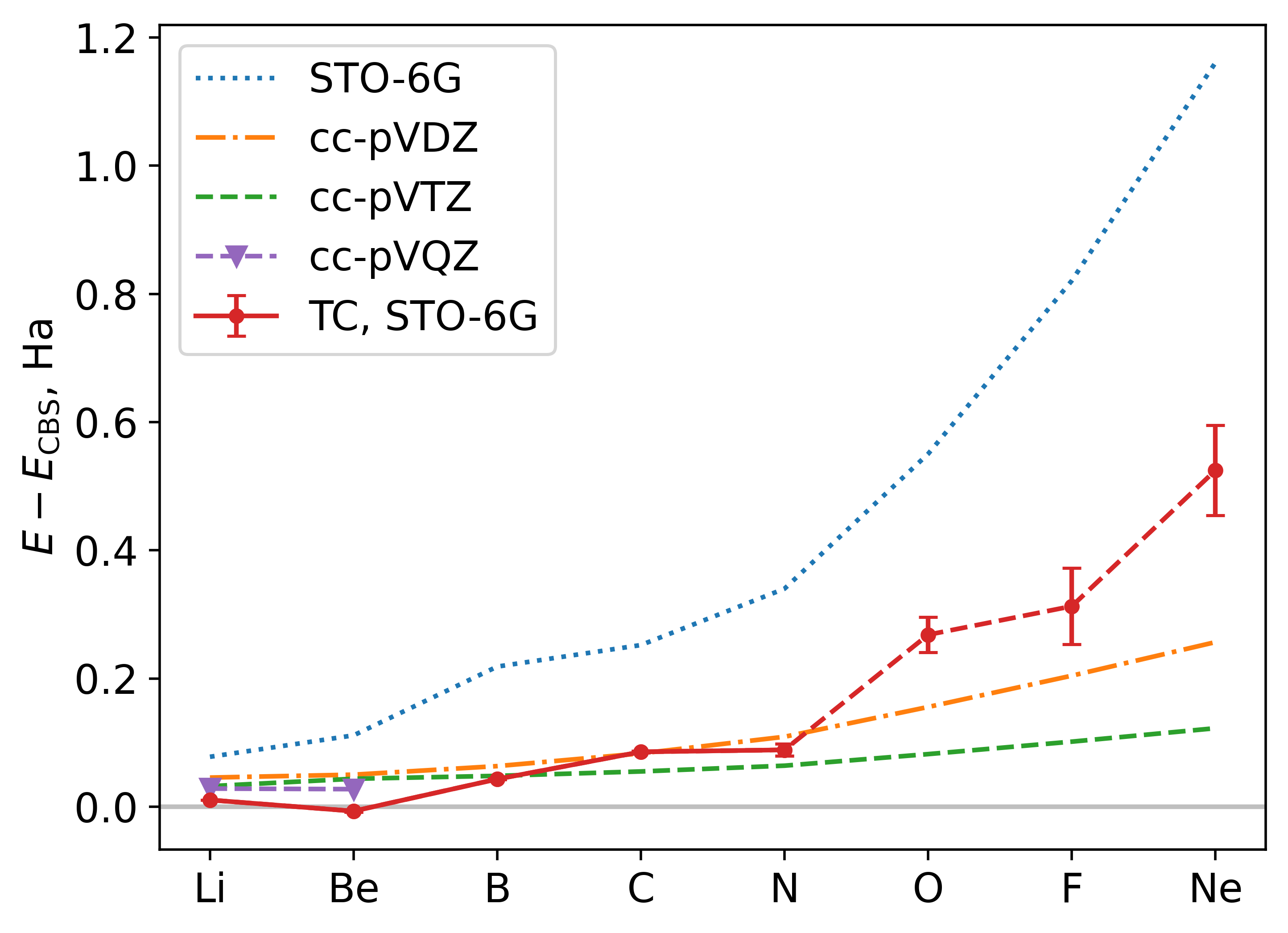
Tables 1 and 2 show the one-norms $\alpha$ and the term counts $K$, respectively. By both measures, the TC Hamiltonians in the STO-6G basis are much smaller than the non-TC Hamiltonians in the cc-pVXZ bases. Moreover, even though the number of terms in the TC Hamiltonians for the STO-6G basis is several times larger than that in the non-TC, STO-6G Hamiltonians, the one-norms have the same order of magnitude.

The randomness in the one-norms is caused by different realizations of the VMC calculation. The number of terms is also random because for the exact TC Hamiltonian in the second-quantized form, we only keep the terms with absolute values of coefficients above $10^{-15}$. We further discard terms according to the threshold that we obtain from (29) when distributing the error budget (denoted as “Truncated TC” in Table 2). In all cases, the threshold was rather small (around $10^{-8}$ to $10^{-7}$ depending on the atom and the instance of VMC calculation), so discarding the terms with weights smaller than that threshold did not affect the one-norms or energies in a noticeable way (the energy changed by $10^{-7}$ Hartree or less). The xTC Hamiltonians did not have any terms that could be discarded this way.

Figure 2 shows the gate counts for performing the qubitization and QEVE for the second-row atoms. While the exact TC method shows gate counts comparable to those of the cc-pVQZ method, the xTC approximation significantly reduces the gate counts, although they still remain above the cc-pVTZ level.

The qubit requirements did not change significantly across different systems. On average, QEVE requires 127.8 logical qubits for the TC Hamiltonians and 118.3 qubits for the xTC Hamiltonians, while standard qubitization requires on average 172.2, 240.2, and 318.1 qubits for cc-pVDZ, cc-pVTZ, and cc-pVQZ bases respectively.

For both algorithms, there is some flexibility in implementing the PREPARE subroutine. The QROAM algorithm ⁴ allows one to reduce the number of T gates at the cost of introducing more ancilla qubits. In Appendix C, we show the T gate and qubit counts for the case when QROAM is optimized for the gate count. In this case, the advantage in gate count is limited, but the qubit count is drastically increased, making this approach impractical.

Figure 3 shows the Jordan condition number of the qubit Hamiltonians across the systems. The truncation of the Hamiltonian that we used for QEVE does not significantly change the condition number. However, the xTC approximation reduces it quite significantly in almost all instances. We calculated $\kappa_{S}$ via exact diagonalization of the Hamiltonian in qubit form: it equals the condition number of the matrix of normalized right eigenvectors.