Scattering in Time-Varying Drude-Lorentz Models

Bryce Dixon bd369@exeter.ac.uk Calvin M. Hooper Ian R. Hooper Simon A. R. Horsley Department of Physics and Astronomy, University of Exeter,
Stocker Road, Exeter, EX4 4QL, UK

Abstract

Motivated by recent experiments, the theoretical study of wave propagation in time varying materials is of current interest. Although significant in nearly all such experiments, material dispersion is commonly neglected in theoretical studies. Yet, as we show here, understanding the precise microscopic model for the material dispersion is crucial for predicting experimental outcomes. Here we study the temporal scattering coefficients of four different time-varying Drude-Lorentz models, exploring how an incident continuous wave splits into forward and backward waves due to an abrupt change in plasma frequency. The differences in the predicted scattering are unique to time-varying media, and arise from the exact way in which the time variation appears in the various model parameters. We verify our results using a custom finite difference time domain algorithm, concluding with a discussion of the limitations that arise from using these models with an abrupt change in plasma frequency.

^†^†preprint: APS/123-QED

I Introduction

The potential for manipulating the frequency spectrum of a wave, to the degree already achieved with spatially structured materials, has motivated recent interest in time-varying media within both photonics and metamaterials communities [Galiffi_2022]. Despite the desire to translate spatial concepts into temporal ones, this field is not simply a replacement $x\to t$ of well established results. For an adiabatic variation of e.g. the refractive index, an incident wave undergoes ‘time refraction’ [Zhou2020, Bohn:21], its frequency shifting with the refractive index, whereas a rapid temporal switch of material parameters leads to ‘time reflection’ [1124533, J_T_Mendonça_2002, Bacot2016, Moussa_2023, Xiao:14] (and even the temporal analogue of an anti–reflection ‘coating’ [Pacheco-Pena:20]). In the latter effect, the constraint of causality requires there is no wave propagating backwards in time, which might be expected from a naive analogy with reflection from a spatial interface. Instead the ‘reflected’ wave propagates forwards in time, but evolves as its time reverse, retracing its motion back to its source (a novel effect, observed in [Bacot2016, Moussa_2023]). Similarly, a periodic modulation of material properties in time leads to a band structure, just as for spatially periodic media. Yet unlike spatially periodic media, where a band gap implies an exponential decay of a propagating wave, a band gap in a temporally modulated medium indicates the onset of parametric amplification, with the wave amplitude growing exponentially in time [1138637, 8434236, Koutserimpas:22]. Topological effects arise in these modulated materials, edge states translating into signals that abruptly transition from being amplified to being absorbed [Lustig:18].

If the material is anisotropic and time–modulated, additional possibilities arise which have only a tenuous analogue in spatially inhomogeneous materials, such as ‘temporal aiming’ [Pacheco-Peña2020], where the direction of propagation is shifted without any spatial boundaries, or the ‘temporal Brewster angle’ [PhysRevB.104.214308], where time reflection vanishes for a particular transition in the material anisotropy. We note that one motivation for this field of research is the possibility of achieving non-reciprocal effects without magnetism [Sounas2017].

Much existing theory, particularly calculations of ‘reflection’ and ‘transmission’ at a temporal interface, is restricted to non-dispersive materials, where the medium is assumed to react instantaneously to the electromagnetic field. However, this is rarely a good approximation, especially in the case of a temporal interface. For example, at near infrared wavelengths a temporal interface implies switching on a femtosecond timescale. Neglecting dispersion is thus equivalent to assuming a material response time that is sub–femtosecond. Yet typical materials such as Indium Tin Oxide have a collision rate on the order of $~200{\,\rm THz}$ , which implies a decay time of the material response of around $5\,{\rm fs}$ . In this example (which is based on the work presented in e.g. [kinsey2015, Jaffray:22, Bohn2021, tirole2022, tirole2023]) it thus seems impossible to neglect dispersive effects.

Assuming a Lorentzian model for the material dispersion, it has been shown that [solís2021timevaryingmaterialspresencedispersion], through conservation of wave–vector $\bm{k}$ , four modes couple at a temporal interface, leading to two forward (positive frequency) and two backward (negative frequency) propagating waves, taking the form of a high and low frequency pair. Unlike the non–dispersive case, where the refractive index is simply a number that we can choose to depend on time, in such a dispersive system we must make some aspect of the material dynamics as time dependent (e.g. the collision rate, the damping constant, the resonant frequency, or the field–medium coupling constant). In [solís2021timevaryingmaterialspresencedispersion], the plasma frequency was taken to vary abruptly, but to model any particular experiment it is far from obvious which parameter to choose (see e.g. [Koutserimpas:24]).

In this work, we calculate electromagnetic wave scattering at a temporal interface for four different choices of explicitly time–varying Drude-Lorentz models, using the Laplace transform method developed in [solís2021timevaryingmaterialspresencedispersion] to derive their temporal scattering coefficients. In general we find the scattering amplitudes vary significantly between the models and are heavily dependent on the initial conditions of both field and medium. However, these differences in the coefficients can be directly related to radiation from ’flashes’ of current at the temporal interface, which arise from quantities that are discontinuous as a consequence of the different boundary conditions implied by the different model choices. As part of these results we discuss some limitations with these models in the limit where the field–medium coupling (here the plasma frequency) is switched to zero. A custom finite difference time domain (FDTD) algorithm was developed to verify the analytical predictions of each of the models. Overall, we show that knowledge of the specific implementation of time–modulation is vitally important when modelling time-varying systems.

II Four Drude–Lorentz Models

Model	Material Dynamics	Continuous Quantities
1	$\frac{d^{2}P(t)}{dt^{2}}+\gamma\frac{dP(t)}{dt}+\omega_{0}^{2}P(t)=\epsilon_{0}\omega_{p}^{2}(t)E(t)$	$\bf{P}$ , $\frac{d\bf{P}}{dt}$ , $\bf{E}$ , $\frac{d\bf{E}}{dt}$ , $\bf{D}$ , $\frac{d\bf{D}}{dt}$
2	$\omega_{p}^{2}(t)\frac{d^{2}}{dt^{2}}\left(\frac{P(t)}{\omega_{p}^{2}(t)}\right)+\gamma\omega_{p}^{2}(t)\frac{d}{dt}\left(\frac{P(t)}{\omega_{p}^{2}(t)}\right)+\omega_{0}^{2}P(t)=\omega_{p}^{2}(t)\epsilon_{0}E(t)$	$\frac{\bf{P}}{\omega_{p}^{2}(t)}$ , $\frac{d}{dt}\left(\frac{\bf{P}}{\omega_{p}^{2}(t)}\right)$ , $\bf{D}$ , $\frac{d\bf{D}}{dt}$
3	$\omega_{p}^{2}(t)\frac{d}{dt}\left(\frac{1}{\omega_{p}^{2}(t)}\frac{dP}{dt}\right)+\gamma\frac{dP}{dt}+\omega_{0}^{2}\omega_{p}^{2}(t)\int_{t_{0}}^{t}\frac{1}{\omega_{p}^{2}(t)}\frac{dP}{dt}dt=\omega_{p}^{2}(t)\epsilon_{0}E(t)$	$\bf{P}$ , $\frac{1}{\omega_{p}^{2}(t)}\frac{d\bf{P}}{dt}$ , $\bf{E}$ , $\bf{D}$ , $\frac{d\bf{D}}{dt}$
4	$\omega_{p}^{2}(t)\frac{d}{dt}\left(\frac{1}{\omega_{p}^{2}(t)}\frac{dP(t)}{dt}\right)+\gamma\frac{dP(t)}{dt}+\omega_{0}^{2}(t)P(t)=\epsilon_{0}\omega_{p}^{2}(t)E(t)$	$\bf{P}$ , $\frac{1}{\omega_{p}^{2}(t)}\frac{d\bf{P}}{dt}$ , $\bf{E}$ , $\bf{D}$ , $\frac{d\bf{D}}{dt}$

Table 1: Polarization dynamics in time–varying Drude–Lorentz models: Here we list the differential equations governing the dynamics of each of our four Drude–Lorentz models, along with the continuous quantities at a temporal discontinuity. We find that all four models must conserve

\bf{D}

and

\frac{d\bf{D}}{dt}

across the boundary.

In this section we introduce our four models for a time–modulated dispersive material, which are summarised in Table 1. Without time–modulation, all models reduce to a standard Drude-Lorentz model where the frequency dependent relative permittivity $\epsilon_{r}$ is given by

\epsilon_{r}=\epsilon_{\infty}+\frac{\omega_{p}^{2}}{\omega_{0}^{2}-\omega^{2}-{\rm i}\gamma\omega},

(1)

with $\mu_{r}=1$ . In the following we assume $\epsilon_{\infty}=1$ and, to obtain tractable analytic results, take a lossless material $\gamma=0$ (see supplementary materials §1 for the effects of $\gamma\neq 0$ ). In all cases we take the time dependence of our system to be induced by an abrupt, instantaneous change in plasma frequency from an initial value, $\omega_{p-}$ , to a final value, $\omega_{p+}$ .

Consider the case of an electromagnetic wave propagating in such a bulk medium. Due to translational symmetry, momentum is conserved and thus the wave–vector $\bm{k}(\omega)=\frac{\omega}{c}\sqrt{\epsilon_{r}}\,\bm{e}_{z}$ must remain unchanged We write this continuity condition as $k_{-}(\omega_{-})=k_{+}(\omega_{+})$ , where the $\pm$ subscript indicates value before ( $-$ ) and after ( $+$ ) the switch. Writing this momentum conservation condition out in terms of the permittivity (1) we thus have,

\frac{\omega_{-}}{c}\sqrt{1+\frac{\omega_{p-}^{2}}{\omega_{0}^{2}-\omega_{-}^{2}}}=\frac{\omega_{+}}{c}\sqrt{1+\frac{\omega_{p+}^{2}}{\omega_{0}^{2}-\omega_{+}^{2}}},

(2)

where we’ve taken $\gamma=0$ as described above. Once squared and the denominators cleared, this leads to a quartic polynomial in $\omega_{+}$ , which can be solved straightforwardly, the roots being given by, {align} ω_+=±ω_n
=±K-(-1)nK2-Δ2(ω-2-ω02), where we have defined,

K=\omega_{-}^{2}(\omega_{-}^{2}+\omega_{p+}^{2}-\omega_{p-}^{2})-\omega_{0}^{2}(\omega_{0}^{2}+\omega_{p+}^{2}),

(3)

and

\Delta=4\omega_{0}^{2}\omega_{-}^{2}(\omega_{-}^{2}-\omega_{0}^{2})(\omega_{-}^{2}-\omega_{0}^{2}-\omega_{p-}^{2}).

(4)

We denote the four roots (2) as $\pm\omega_{1}$ and $\pm\omega_{2}$ , as defined in Eq. (2). If the plasma frequency varies suddenly in time then before and after this modulation, the wave will be in some superposition of these four frequencies. We now proceed to show that the amplitudes in this superposition are heavily dependent on the model of the material dynamics used to describe the time modulation (see the schematic in Fig. 1). We now summarize these four Drude–Lorentz models.

Refer to caption — Figure 1: Time–varying Drude-Lorentz models: At each point $z$ within the medium an incident field couples to the harmonic motion of the polarization $\bm{P}$ , with charge $q_{e}$ , effective mass $m^{\star}$ , resonant frequency $\omega_{0}$ , and damping $\gamma$ . The coupling into the motion is proportional to $\kappa_{\rm in}$ , and the coupling back out into the field is proportional to $\kappa_{\rm out}$ . For an abrupt change in the material parameters, we can achieve fixed initial and final permittivities, $\epsilon(\omega)$ through changing different combinations of these model parameters. In model 1, the time modulation occurs through the ‘in–coupling’, $\kappa_{\rm in}(t)$ , in models 2 and 3 through the ‘out–coupling’, $\kappa_{\rm out}(t)$ , and in model 4, through the effective mass, $m^{\ast}(t)$ .

II.1 Model 1: modulated in–coupling

We use the standard Drude–Lorentz model as our starting point. Here the polarization $\bm{P}(t)=\bm{e}_{x}P(t)$ obeys the equation of a damped simple harmonic oscillator with damping constant $\gamma$ , resonant frequency $\omega_{0}$ , and a coupling to the electric field proportional to the plasma frequency $\omega_{p}$ ,

\frac{d^{2}P(t)}{dt^{2}}+\gamma\frac{dP(t)}{dt}+\omega_{0}^{2}P(t)=\epsilon_{0}\omega_{p}^{2}E(t).

(5)

In Ref. [solís2021timevaryingmaterialspresencedispersion], the time modulation of the material response is introduced through assuming a time-dependent plasma frequency $\omega_{p}(t)$ , considering this to be equivalent to an abrupt change in the electron number density. The time-dependent plasma frequency is then defined as,

\omega_{p}(t)=\sqrt{\frac{q_{e}^{2}n(t)}{m^{*}\epsilon_{0}}},

(6)

where $q_{e}$ is the electron charge, $m^{*}$ is the effective mass of the charge carriers, and $n(t)$ is the time-dependent electron number density given as $n(t)=n_{-}+(n_{+}-n_{-})\Theta(t)$ , where $\Theta(t)$ is the Heaviside step function. The step function approximation holds for real systems, provided the duration of the change is sufficiently shorter than the period of the wave. Our first time–varying model for the polarization is therefore,

\frac{d^{2}P(t)}{dt^{2}}+\gamma\frac{dP(t)}{dt}+\omega_{0}^{2}P(t)=\epsilon_{0}\omega_{p}^{2}(t)E(t),

(7)

with Maxwell’s equations unmodified. Without singularities in the external current, Maxwell’s equations imply that the $\bm{D}$ and $\bm{B}$ fields are continuous across a time interface [Galiffi_2022], and from Eq. (7) we observe—demanding that all time derivatives are finite—that the polarization and its time–derivative must also be continuous in this particular model. Through using the relation $\bm{D}=\epsilon_{0}\bm{E}+\bm{P}$ , we thus also have continuity of $\bm{E}$ and $d\bm{E}/dt$ , despite the carrier density $n(t)$ being discontinuous.

With reference to Fig. 1, we observe that this model can be understood as a simple harmonic oscillator with a time–varying in–coupling $\kappa_{\rm in}(t)$ , of the field into the oscillatory motion, but a constant fixed out–coupling $\kappa_{\rm out}$ of the motion into radiation.

Note that, although we are writing the equations here in terms of electromagnetic parameters relevant for a condensed matter, or radio frequency metamaterial system, almost identical equations hold in acoustic systems, where constitutive relations can also be varied in time. In that context, this first model is closely related to the time–modulated meta–atoms described in [Cho2020], where a time–varying Drude–Lorentz response is achieved through modulating the in–coupling to the meta–atom (in– and out–coupling here are respectively the volume of a speaker and microphone, coupled through a single–board computer).

II.2 Model 2: modulated polarization density

As the converse of model 1, we can envisage a situation where the in–coupling to the polarization field is fixed as $\kappa_{\rm in}$ , while the out–coupling to the radiation $\kappa_{\rm out}(t)$ , changes in time. As we shall show, this choice has an effect on the frequency conversion when the permittivity is rapidly modulated, although the initial and final form of the frequency dependent permittivity is identical between the models. Again, although we develop our formalism for electromagnetic waves, this situation can be implemented using the acoustic meta–atoms described in [Cho2020], where the output volume of the speaker is varied in time.

We motivate this model through considering an individual charge of fixed effective mass $m^{\ast}$ , at position $x(t)$ , and undergoing harmonic motion, subject to the electric field, $\bm{E}=E\bm{e}_{x}$ ,

\frac{d^{2}x(t)}{dt^{2}}+\gamma\frac{dx(t)}{dt}+\omega_{0}^{2}x(t)=\frac{q_{e}}{m^{*}}E(t).

(8)

We then introduce the polarisation $\bm{P}$ as the net dipole moment per unit volume inside the material, taking the density of carriers $n(t)$ to change in time such that,

{\bm{P}}(t)=n(t)q_{e}x(t)\,\bm{e}_{x}.

(9)

Combining the equation for the motion of the charge \eqrefelectron_pos with the definitions of both the polarization \eqrefmod2P and the plasma frequency \eqrefeq:omega_p, results in a differential equation in governing the evolution of the polarization, {multline} ω_p^2(t)d2dt2(P(t)ωp2(t))+γω_p^2(t)ddt(P(t)ωp2(t))
+ω_0^2P(t)=ω_p^2(t)ϵ_0E(t), which is identical to \eqrefmodel 1 when the plasma frequency is constant, reducing to the standard Drude–Lorentz model \eqrefengheta. However, examining \eqrefmod2P, we can see that the continuous quantities are $\bm{P}/\omega_{p}^{2}$ and $d(\bm{P}/\omega_{p}^{2})/dt$ . Given the continuity of $\bm{D}$ and $\bm{B}$ implied by Maxwell equations, a sudden switch in the plasma frequency results in a discontinuous $\bm{E}$ and $d\bm{E}/dt$ here. As we shall see, this difference in the boundary conditions leads to very different temporal scattering coefficients. This version of the time-varying Drude-Lorentz model was used in Ref. [PhysRevA.111.033507].

II.3 Model 3: modulated current density

Another version of model 2, where we vary the ‘out–coupling’ in time, is written in terms of the current density $j=dP/dt$ , rather than the polarization,

\frac{dP(t)}{dt}=q_{e}\,n(t)\frac{dx(t)}{dt},

(10)

where the current is given by the instantaneous carrier density $n(t)$ , times the carrier charge and velocity. This version of the time–varying Drude–Lorentz model was used in Ref. [PhysRevLett.130.203803]. For static materials, Eq. \eqrefmod3P is simply the time derivative of \eqrefmod2P, again making the two models equivalent. Using the expression for the current \eqrefmod3P to write the equation of motion \eqrefelectron_pos in terms of the polarization field we now have an integro–differential equation for the polarization field, {multline} ω_p^2(t)ddt(1ωp2(t)dPdt)+γdPdt+
ω_0^2ω_p^2(t)∫_t_0^t 1ωp2(t)dPdtdt=ω_p^2(t)ϵ_0E(t). where we take the boundary condition that the displacement $x(t)$ vanishes at time $t=t_{0}$ . Again, Eq. \eqrefmodel 3 reduces to the standard Drude–Lorentz model when $\omega_{p}$ is time independent. However, note that the integral term makes the dynamics explicitly dependent on the history of the polarization field. From an examination of \eqrefmodel 3, both $P$ and $(1/\omega_{p}^{2})\,dP/dt$ are continuous functions of time, implying that—for an abrupt change in plasma frequency—the electric field is continuous, while its time derivative is not.

II.4 Model 4: modulated effective mass

Finally we take the plasma frequency to vary through a change in the effective mass, $m^{\ast}$ of the charge carriers. We modify the equation of motion \eqrefelectron_pos, remembering that the rate of change of momentum is given by $d(m^{\ast}\,dx/dt)/dt$ . Thus,

\frac{d}{dt}\left(m^{*}(t)\frac{dx(t)}{dt}\right)+\gamma m^{*}(t)\frac{dx(t)}{dt}+\mathcal{K}x(t)=q_{e}E(t),

(11)

where $\mathcal{K}(t)=m^{\ast}(t)\omega_{0}^{2}$ is the spring constant.

Following the same procedure described in the three previous cases and using \eqrefmod2P to write the dynamics of the polarization field (taking constant value of carrier density $n$ in this model), this leads to, {multline} ω_p^2(t)ddt(1ωp2(t)dP(t)dt)+γdP(t)dt+
ω_0^2 P(t)=ϵ_0ω_p^2(t)E(t). Interestingly, when the resonant frequency $\omega_{0}$ equals zero, this model is equivalent to the modulated carrier density described in model 3. As the term proportional to $\omega_{0}$ in Eqns. \eqrefmodel 3 and \eqrefmodel 4 plays no role in determining the continuity conditions, the temporal boundary conditions here are identical to those in model 3.

III Scattering Coefficients

We now consider a plane wave of initial wave–vector $\bm{k}$ and frequency $\omega_{-}$ propagating in an infinite bulk medium where the polarization evolves according to one of the four models outlined in the previous section. At $t=0$ the plasma frequency is rapidly switched from the value $\omega_{p-}$ to the value $\omega_{p+}$ , causing the wave to scatter into the four different frequencies given by Eq. \eqrefquartic. To find the scattering amplitudes we use the Laplace transform method described in Ref. [solís2021timevaryingmaterialspresencedispersion]. The full derivation of these amplitudes for each model are given in supplementary materials §3.

We start from the vector wave equation obtained by eliminating the magnetic field from the two Maxwell equations involving curls,

\bm{\nabla}\times(\bm{\nabla}\times\bm{E})=-\mu_{0}\epsilon_{0}\frac{\partial^{2}\bm{E}}{\partial t^{2}}-\mu_{0}\frac{\partial^{2}\bm{P}}{\partial t^{2}}.

(12)

As the wave–vector is conserved in a homogeneous medium, we can make the replacement $\bm{\nabla}={\rm i}\bm{k}={\rm i}k\bm{e}_{z}$ , assume the fixed polarization, $\bm{E}=E\bm{e}_{x}$ and $\bm{P}=P\bm{e}_{x}$ , and thus reduce (12) to,

\left(c^{2}k^{2}+\frac{d^{2}}{dt^{2}}\right)\epsilon_{0}E=-\frac{d^{2}P}{dt^{2}}.

(13)

Taking the Laplace transform of Eq. (13) over all positive times $t>0$ , we have, {multline} (c^2k^2+s^2)ϵ_0 ~E(s) = ϵ_0 s E(0^+)+ϵ_0dEdt(0^+)
-s^2~P(s)+sP(0^+)+dPdt(0^+). where $s$ is the Laplace transform variable, conjugate to time, and $0^{\pm}$ indicate infinitesimal positive/negative quantities. Note that Eq. (13) represents the transform of the field and polarization after the switch, where the medium is not changing any more. The conversion between frequencies at the time boundary is thus entirely wrapped up in the connection between the electric field and polarization amplitudes and their time derivatives before and after the rapid change in plasma frequency (i.e. evaluated at the times $0^{+}$ and $0^{-}$ ).

To eliminate $\tilde{P}(s)$ from Eq. (13), we perform a second Laplace transform on one of the differential equations for the polarization dynamics, either Eqn. \eqrefmodel 1, \eqrefmodel 2, \eqrefmodel 3, or \eqrefmodel 4. However, for times after the switch, all of these differential equations reduce to the standard Drude–Lorentz model for a static medium \eqrefengheta. Note that in model 3 this requires the boundary condition that the polarization and its time derivative vanish at $t=-\infty$ , as discussed in supplementary materials §3. This results in an algebraic equation we can solve for the polarization, the solution of which is,

\tilde{P}(s)=\frac{\epsilon_{0}\omega_{p+}^{2}\tilde{E}(s)+sP(0^{+})+\frac{dP}{dt}(0^{+})}{s^{2}+\omega_{0}^{2}}+\xi

(14)

where $\xi=0$ for models 1, 2 and 4. Performing this Laplace transform over the integral term in model 3 results in $\xi=\frac{\omega_{0}^{2}}{s(s^{2}+\omega_{0}^{2})}\left(P(0^{+})-\frac{\omega_{p+}^{2}}{\omega_{p-}^{2}}P(0^{-})\right)$ . Substituting this into equation \eqreflaplace_field_eq we find the relation between the Laplace amplitude of the electric field, and the values of the field and polarization immediately after the switch in the plasma frequency, {multline} [(c^2 k^2+s^2)(ω_0^2+s^2)+s^2ω_p+^2]~E(s)
=(s^2+ω_0^2)[sE(0^+)+dEdt(0^+)]
+ω02ϵ0[sP(0^+)+dPdt(0^+)] - s2(s2+ω02)ϵ0ξ. Before the abrupt change in the plasma frequency at $t=0$ , we take the electric field as a unit amplitude travelling wave, and find the polarization as the inhomogeneous solution to Eq. (7) with a constant value of the plasma frequency $\omega_{p}=\omega_{p-}$ . These expressions are, {align} E(t¡0)=cos(kz-ω_-t)
P(t¡0)=ϵ0ωp-2ω02-ω-2cos(kz-ω_-t). Taking the time $t=0^{-}$ , just before the discontinuous jump in the plasma frequency, Eq. (14) shows that $E(0^{-})=\cos(kz)$ ; $\left.dE/dt\right|_{0^{-}}=\omega_{-}\sin(kz)$ ; $P(0^{-})=\epsilon_{0}\omega_{p-}^{2}\cos(kz)/(\omega_{0}^{2}-\omega_{-}^{2})$ ; and $\left.dP/dt\right|_{0^{-}}=\epsilon_{0}\omega_{-}\omega_{p-}^{2}\sin(kz)/(\omega_{0}^{2}-\omega_{-}^{2})$ . Table 1 then tells us how to relate these values to those after the jump in plasma frequency. These values are given in Table 2.

Quantity	Model 1	Model 2	Model 3	Model 4
$E(0^{+})=$	$\cos(kz)$	$\left(1+\frac{\omega_{p-}^{2}-\omega_{p+}^{2}}{\omega_{0}^{2}-\omega_{-}^{2}}\right)\cos(kz)$	$\cos(kz)$	$\cos(kz)$
$\frac{dE}{dt}(0^{+})=$	$\omega_{-}\sin(kz)$	$\left(1+\frac{\omega_{p-}^{2}-\omega_{p+}^{2}}{\omega_{0}^{2}-\omega_{-}^{2}}\right)\omega_{-}\sin(kz)$	$\left(1+\frac{\omega_{p-}^{2}-\omega_{p+}^{2}}{\omega_{0}^{2}-\omega_{-}^{2}}\right)\omega_{-}\sin(kz)$	$\left(1+\frac{\omega_{p-}^{2}-\omega_{p+}^{2}}{\omega_{0}^{2}-\omega_{-}^{2}}\right)\omega_{-}\sin(kz)$
$P(0^{+})=$	$\frac{\epsilon_{0}\omega_{p-}^{2}}{\omega_{0}^{2}-\omega_{-}^{2}}\cos(kz)$	$\frac{\epsilon_{0}\omega_{p+}^{2}}{\omega_{0}^{2}-\omega_{-}^{2}}\cos(kz)$	$\frac{\epsilon_{0}\omega_{p-}^{2}}{\omega_{0}^{2}-\omega_{-}^{2}}\cos(kz)$	$\frac{\epsilon_{0}\omega_{p-}^{2}}{\omega_{0}^{2}-\omega_{-}^{2}}\cos(kz)$
$\frac{dP}{dt}(0^{+})=$	$\frac{\epsilon_{0}\omega_{-}\omega_{p-}^{2}}{\omega_{0}^{2}-\omega_{-}^{2}}\sin(kz)$	$\frac{\epsilon_{0}\omega_{-}\omega_{p+}^{2}}{\omega_{0}^{2}-\omega_{-}^{2}}\sin(kz)$	$\frac{\epsilon_{0}\omega_{-}\omega_{p+}^{2}}{\omega_{0}^{2}-\omega_{-}^{2}}\sin(kz)$	$\frac{\epsilon_{0}\omega_{-}\omega_{p+}^{2}}{\omega_{0}^{2}-\omega_{-}^{2}}\sin(kz)$

Table 2: Field amplitudes immediately after the time boundary: Electric field, polarization, and their time derivatives immediately after an abrupt change in the plasma frequency, from

\omega_{p-}

\omega_{p+}

t=0

. These values determine the Laplace amplitude of the electric field via Eq. (14).

After substituting the values listed in Table 2 into Eq. (14), we have completely determined the electric field in all of the models, before and after the switch in plasma frequency. Performing the inverse Laplace transform using the expression for $\tilde{E}(s)$ given in \eqrefeq:laplace-E we have {align} E(t)=∫_-i∞+Γ^i∞+Γds2πi ~E(s) e^st
=F(s1) es1t-F(-s1) e-s1t2s1(s22-s12)
-F(s2)es2t-F(-s2)e-s2t2s2(s22-s12) where $\Gamma$ is a number we choose to ensure the convergence of the integral, we have defined $F(s)=(s^{2}+\omega_{0}^{2})[sE(0^{+})+dE/dt(0^{+})]+\epsilon_{0}^{-1}\omega_{0}^{2}[sP(0^{+})+dP/dt(0^{+})]-\epsilon_{0}^{-1}s^{2}(s^{2}-\omega_{0}^{2})\xi$ , and $\pm s_{1}$ and $\pm s_{2}$ are the four imaginary roots of the polynomial $(c^{2}k^{2}+s^{2})(\omega_{0}^{2}+s^{2})+s^{2}\omega_{p+}^{2}=0$ . In Fig. 2 we show the contour used to evaluate the integral in Eq. \eqrefeq:inverse_laplace_result. The quantity $F$ within each of the terms within Eq. (III) depends on the initial values of the electric field and polarization, which—as we have already discussed—are model dependent.

We can see that Eq. \eqrefeq:inverse_laplace_result is a solution to the wave equation of the form,

E(t)=E_{1}^{+}+E_{1}^{-}+E_{2}^{+}+E_{2}^{-}.

(15)

with each wave evolving in time with the frequency $\pm\omega_{1,2}$ defined in Eq. \eqrefquartic. The amplitudes of each of these waves are the four temporal scattering coefficients.

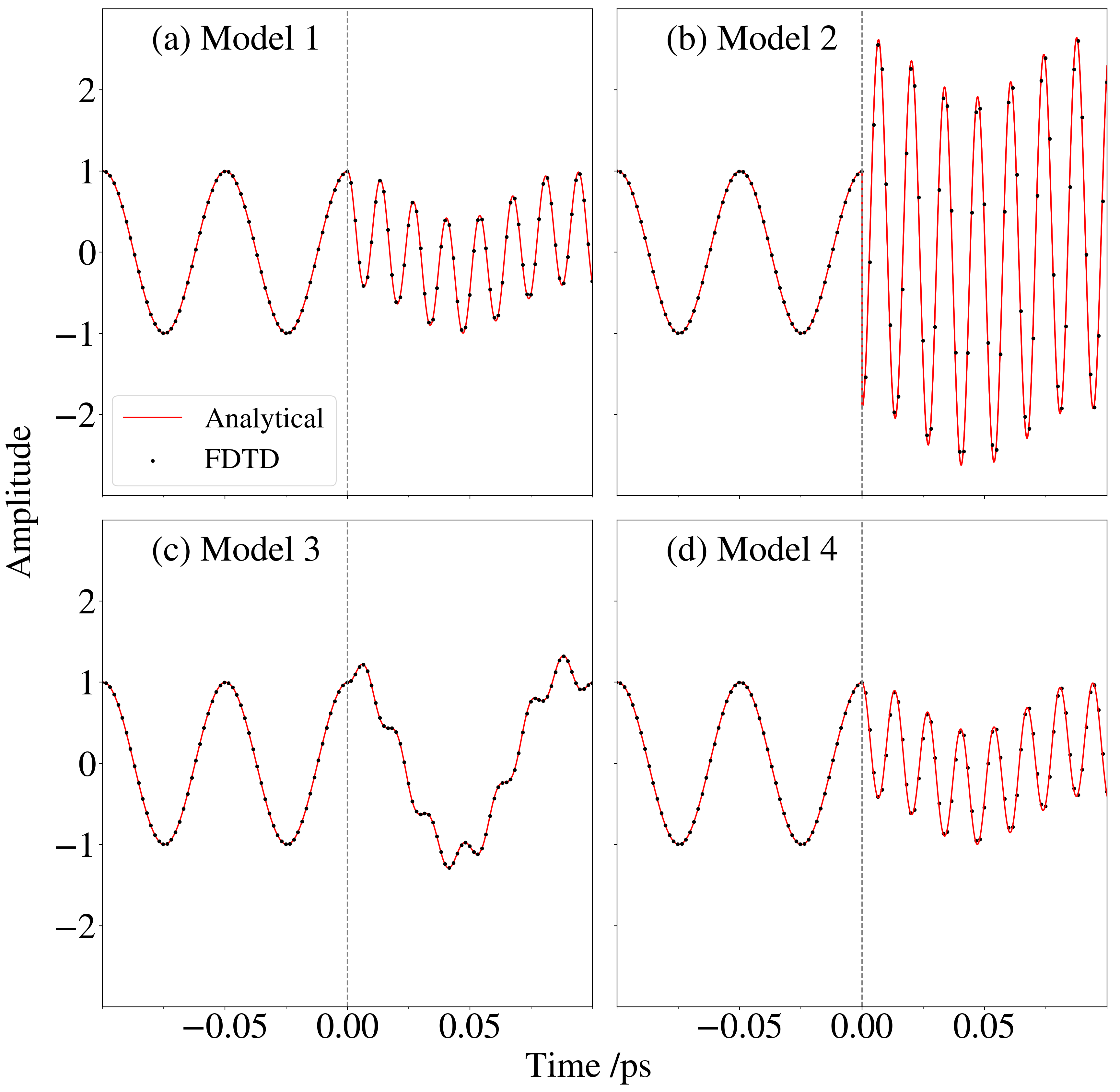
To verify these solutions, we used a custom finite difference time domain (FDTD) algorithm for each of the Drude-Lorentz models. To examine the scattering coefficients, we injected a single frequency wave with unit amplitude into a material with plasma frequency $\omega_{p-}$ . After a time $t_{0}$ , the plasma frequency of the entire system was instantaneously switched to $\omega_{p+}$ , and the amplitudes and frequencies of the four scattered waves were compared to those of the theory. Figure 3 shows the electric field output of the FDTD simulation in the time domain over-plotted with the predicted electric field solution according to the Laplace transform theory for each model for a particular set of system parameters. We see that our analytical solutions are in direct agreement with the simulation for all four models.

IV Comparison between models: emission at the interface

Whilst the full electric field after the jump in plasma frequency is given in Eq. \eqrefeq:inverse_laplace_result, we now compare the scattering coefficients of all four models relative to model 1, which was that used in Ref. [solís2021timevaryingmaterialspresencedispersion]. Here, we refer to the forward and backward scattering coefficients representing the waves with frequencies $\pm\omega_{1}$ and $\pm\omega_{2}$ as $A_{1,2}^{\pm}$ . We denote the scattering coefficients for a particular model with a Roman numeral (I, II, III, or IV). Firstly the waves travelling with $\pm\omega_{1}$ are given by {align} A_1,II^±= A_1,I^±+ (ω12±ω-ω1)(ωp+2-ωp-2)2(ω-2-ω02)(ω12-ω22),
A_1,III^±= A_1,I^±+ (ω02±ω-ω1)(ωp+2-ωp-2)2(ω-2-ω02)(ω12-ω22),
A_1,IV^±= A_1,I^±±ω-ω1(ωp+2-ωp-2)2(ω-2-ω02)(ω12-ω22). Similarly, the scattering coefficients for the waves travelling with $\pm\omega_{2}$ equal {align} A_2,II^±= A_2, I^±- (ω22±ω-ω2)(ωp+2-ωp-2)2(ω-2-ω02)(ω12-ω22),
A_2,III