\pagerange

Lord of the (sub-)Rings : Mapping the surface reflectance and spin-axis of Ajisai–B

Lord of the (sub-)Rings : Mapping the surface reflectance and spin-axis of Ajisai

Robert J. S. Airey ^1,2 Paul Chote E-mail: Robert.Airey@warwick.ac.uk ^1,2 James A. Blake ^1,2 James McCormac ^1,2 Billy Shrive ^1,2 Don Pollacco ^1,2 Benjamin F. Cooke^1,2
¹Department of Physics University of Warwick Gibbet Hill Road Coventry CV4 7AL UK
²Centre for Space Domain Awareness University of Warwick Gibbet Hill Road Coventry CV4 7AL UK

(2026)

Abstract

Active debris removal techniques are posed to become an important tool in maintaining the safety of the near-Earth space environment. These techniques rely on a clear understanding of the rotational motion of the debris targets, which is challenging to constrain from unresolved imaging. The Ajisai satellite provides an ideal test case for developing and demonstrating these techniques due to its simple geometry and well constrained spin behaviour. We present four observations of the Ajisai satellite taken with SuperWASP in August of 2019, where high cadence photometry was extracted from streaked images as a part of a larger survey of Low Earth Orbit. We develop an MCMC-driven method to determine the spin-state of Ajisai by comparing the alignment between a map of modelled mirror positions and a novel derived map of surface reflectivity. We generally find good agreement within the expectation and uncertainties set by empirical models and our determined spin-state solutions align the surface reflectivity map and modelled mirror location well. Our results show that streak photometry can be used to recover the spin-axis and rotation period of fast-spinning objects such as Ajisai using modest ground-based instrumentation, making it readily scalable to a wider range of targets and observatories.

keywords:

Satellites – Instrumentation – Photometry – Data Methods

1 Introduction

The population of non-cooperative objects in the near-Earth environment has continued to grow in recent years (Blake, 2022; Serrano et al., 2024), such that active debris removal (ADR) techniques to achieve a more sustainable space and reduce collision risk are being proactively proposed and discussed (see e.g. Endo et al., 2022; Boonrath et al., 2024; Rossi et al., 2024; Sampath and Feng, 2024). In particular, most ADR techniques rely on a service vehicle to attach itself to the debris target; therefore, it is critical that the rotational state of the debris object be known.

Using photometric measurements with the aim of estimating the state (spin-axis and period) of a non-cooperative object has become an active area of research (see e.g. Šilha et al., 2018; Blake et al., 2021; Laurence, 2022; Meyer et al., 2024). However, these techniques may rely on a BRDF (Bidirectional Reflectance Distribution Function) model (Hapke, 2012) being implemented to generate synthetic light curves which can be compared to truth observed light curves. Although, more recent methods have been developed which can infer spin properties directly from temporal frequency changes without assuming a particular BRDF (see e.g. Zhao et al., 2020; Badura and Valenta, 2024).

This study aims to determine the attitude state of the Ajisai satellite purely from TLE-derived vectors and high-cadence optical photometry, expanding on the previous work by Hall et al. (2006) (Epoch-method) and, more recently, by Koshkin et al. (2024) (photometric-patterns method). It is important to note that Ajisai’s spin state has been previously investigated using different approaches. Notably, Calatroni et al. (2025) employed high-frequency optical photometry (5–10 kHz) to determine the full rotation state—including the spin axis, period, and initial rotation phase—with high single-pass accuracy. Kucharski et al. (2016) achieved long-term monitoring of Ajisai’s attitude evolution using 2 kHz Satellite Laser Ranging (SLR) data which benefits from much broader temporal coverage at a high precision. Earlier optical studies such as Koshkin et al. (2017), demonstrated that attitude determination can also be performed with modest ground-based instrumentation, and therefore this work is particularly relevant as a precursor to the present study. The reflectivity of the Ajisai mirrors have also been studied in the works of Kucharski et al. (2019b) and Kucharski et al. (2020) in which the focus is purely on studying the mirror reflectivity mapping as opposed to attitude determination.

Observational cadences on the order of milliseconds are needed to ascertain the spin-states of the fastest spinning objects (Kucharski et al., 2019a), which places strict limits on observing cadence with traditional CCD observations due to their relatively slow readout times and inefficiency at capturing rapid exposures without introducing significant dead time. Here we present a technique that doesn’t rely on specialized kHz-level instrumentation, making it more readily scalable to a wider range of targets and observatories.

1.1 Ajisai Background

Refer to caption — Figure 1: The Ajisai satellite with mirror panels and CCRs (corner cube reflectors) covering its spherical surface labelled on the figure. This figure is taken from Otsubo et al. (2000)

The Ajisai satellite (NORAD: 16908, COSPAR: 1986-061A) was launched in 1986 as part of a geodetic mission sponsored by the NASDA (National Space Development Agency of Japan), with the goal of improving the accuracy of domestic geodetic triangulation with respect to other networks and accurately measuring the position of the remote Japanese islands (McDowell, 2002). The satellite is in Low Earth Orbit (LEO) approximately 1500 km above the Earth’s surface with an orbit inclined by approximately 50^∘. Ajisai is a 685 kg hollow sphere with a diameter of 2.15 meters, and the surface is covered with 318 mirrors and 1436 corner-cube retroreflectors (CCRs)(Sasaki and Hashimoto, 1987) (see Figure 1). Work done in Kirchner et al. (2007) determined that Ajisai is spinning in the clockwise direction. The mirrors of Ajisai are curved at a radius of 8.55 m ( $\pm$ 0.15) and have a surface area of up to 393 cm² each (Kucharski et al., 2019b). There are two modes of operation that enable precise geodetic measurements: one involves sending a ground-based laser beam to the satellite’s CCRs and measuring the round-trip travel time (laser ranging); the other involves imaging the illuminated satellite from ground stations against background stars to determine its position (eoPortal – Earth Observation Portal, 2012).

The mirrors covering the surface are organized into 12 primary latitudinal rings, along with two polar caps. Each primary ring is composed of several sub-rings, with each sub-ring containing three mirrors positioned at the same latitude and inclined in the same latitudinal direction. This means that within a given revolution of the object around its spin-axis, a sub-ring of mirrors should always be able to reflect light towards an observer.

Ajisai was spin-stabilised, with an initial spin vector aligned with the Earth’s rotation and a period of 1.5 s (Sasaki and Hashimoto, 1987). The spin-axis in the International Celestial Reference Frame (ICRF) and period of Ajisai at any time of observation can be approximated using the empirical models from Kucharski et al. (2016). These are a set of time-dependent equations which describe the expected evolution of the precession and nutation cones of the spin-axis, and the period as an exponential trend function. The expected evolution of the spin state of Ajisai in accordance with the empirical models is shown in Figure 2. The equations to calculate the spin-axis vector and period are given in Appendix A.

2 Instrumentation and Observations

The SuperWASP (Super Wide Angle Search for Planets) project (Pollacco et al., 2006) was a highly successful ground-based exoplanet survey. Operating from 2004 until 2018, it discovered and confirmed nearly 200 transiting Hot Jupiter class planets. The survey operated two custom survey telescopes (SuperWASP North on La Palma and SuperWASP South in South Africa) that used an array of consumer telephoto lenses (the Canon EF 200mm f/1.8L USM) with scientific CCD cameras to provide an instantaneous field of view of nearly 500 deg² for each telescope.

Between 2018 – 2022, SuperWASP North (hereafter just SWASP) was used for several observational Space Domain Awareness (SDA) research projects. A picture of SWASP during this period is shown in Figure 3.

The SuperWASP project was searching for transit signals that occur on timescales of minutes to hours; as such, it was not designed to support the sub-second timestamp accuracy required when observing fast-moving LEO satellites. In particular, variable timing delays between the Telescope Control Server (TCS) and the individual Data Acquisition Servers (DASes) for each camera meant that the individual mosaic sub-exposure start times could differ by more than a second. A further problem arose from the dated Scientific Linux 3 operating system that was not compatible with modern scientific software libraries.

These issues were resolved by introducing a Raspberry Pi single-board computer to control observations. A custom control daemon (implemented using Python) parsed an observation plan file (containing a list of positions and times) and issued shell commands via SSH to custom helper programs (implemented using C) on the TCS that then called the original SWASP control system scripts to point the mount and prepare exposures. Custom circuitry, extending the principles of an earlier instrument, Puoko-nui (Chote et al., 2014), generated a GPS-timestamped TTL pulse to simultaneously trigger the cameras using their external trigger input. The timestamps and associated exposure IDs were saved to the observing plan file where they could be reconciled during subsequent processing. Figure 4 provides a high-level overview of this modified system.

By 2018, only six of the original eight CCD cameras were operational. These were realigned using the per-camera adjustments available on the mount, with four cameras forming a square $16^{\circ}\times 16^{\circ}$ field of view and the remaining two cameras overlapping the central field to provide redundancy and to enable cross-validation between cameras.

2.1 LEO Survey

The modified SWASP undertook a survey of LEO resident space objects (RSOs) between July – November 2019, and captured in total 1826 passes of 774 individual RSOs.

The Observatorio del Roque de Los Muchachos on La Palma is an excellent dark-sky site (2349 m altitude; V_sky $\sim$ 22 mag/arcsec²), but the large angular size of the SuperWASP pixels meant that the effective sky background during dark conditions was V_sky $\sim$ 16.5 mag. This limited its usefulness to observing stars brighter than V $\sim$ 15 (Pollacco et al., 2006), but was well matched to the population of TLE-catalogued LEO RSOs, which are generally V $\lesssim$ 12 mag.

The path of a target RSO across the sky was divided into a set of precisely timed sidereal fields that capture the target shortly after it entered the field of view, and completed shortly before it left. The exposure time for each field was determined by the time it took the RSO to cross the field, which was typically a few seconds (and limited to a maximum of 45 seconds to avoid saturation of background stars).

High time resolution light curves were extracted by measuring the change in surface brightness along the length of the streak; the effective time resolution was set by the time it takes the target to move by a point-spread-function width across the CCD; of order tens of milliseconds at typical LEO altitudes for SuperWASP’s 13 arcsecond pixel size.

Each exposure was separated by a 15 second delay, during which the CCDs were read out and the mount repositioned to the next field. The same sidereal pointings were observed for a second time immediately after each pass (generally within $5-10$ minutes, minimising any potential changes in sky transparency) to provide reference images of the sky behind the target streaks. Difference images were created using hotpants (Becker, 2015) to align, resample, and subtract the images. Pixels associated with bright sources in the reference image were masked in the difference image to reduce false signals introduced by residual difference artifacts.

Figure 5 illustrates the observation procedure, which was described in detail, along with the data reduction pipeline, in Chote et al. (2019).

2.2 Ajisai Observations

Ajisai was observed 4 times between the nights of the 2019 August 1 – 16. Figure 7 and Table 1 provide a summary of these data.

The rate of motion of Ajisai compared to the background stars changes during each pass, producing a time resolution that is continuously changing. Figure 6 illustrates that the typical time resolution is $100-150\,$ ms: an order of magnitude larger than the $\sim 10\,$ ms wide glint features (Calatroni et al., 2025). The photometric map methodology described in Section 3 is sensitive primarily to the spacing between glints, so it is not necessary to resolve the individual glints.

Table 1: Summary of our 2019 SuperWASP observations of Ajisai.

D_{\text{obs}}

N_{\text{data}}

and

N_{\text{fields}}

refer to the number of days since launch (

D_{\text{launch}}=46654.86

[MJD]), the number of observed datapoints and the number of sidereal fields the satellite was observed in respectively.

$T_{\text{start}}$ [UTC]	$T_{\text{end}}$ [UTC]	$D_{\text{obs}}$ [Days]	$N_{\text{data}}$	$N_{\text{fields}}$
2019-08-02 3:25:03	2019-08-02 3:29:38	12042.28	6787	5
2019-08-03 2:33:25	2019-08-03 2:35:18	12043.25	3665	3
2019-08-08 2:06:06	2019-08-08 2:07:55	12048.23	1597	2
2019-08-16 23:56:23	2019-08-17 00:05:42	12057.14	6224	7

3 Methodology

The procedure for extracting the spin-axis and period of Ajisai from our photometric observations can be broadly broken down into the following steps:

1.

Defining a function that calculates (from an input Two Line Element ephemeris) the Phase Angle Bisector (PAB) vector in the ICRF reference frame (see section 3.1) as a function of input time.
2.

Defining a function that transforms the PAB unit vectors, for a chosen set of rotation parameters (spin-pole coordinates, period and a rotational phase offset), into the RSO body fixed frame.
3.

Using these two functions to map each measurement in the light curve, for a chosen set of rotation parameters, to a latitude and longitude on the surface of Ajisai.
4.

Comparing the resulting two dimensional glint positions against the known mirror positions and using a MCMC (Markov Chain Monte Carlo) search to find the parameters (and associated uncertainties) that produce the best alignment.

The result of this procedure is a two dimensional brightness map that visualises the surface reflectivity of Ajisai. The position of each mirror (strictly speaking, the orientation of its normal vector) is clearly visible by a localised spike in brightness centered on its position.

3.1 Reference Frame Transformation and Vector Calculations

The PAB, p, is defined as the unit vector halfway between the satellite-to-Sun ( $V_{\text{sat$\rightarrow$ Sun}}$ ) and satellite-to-observer directions ( $V_{\text{sat$\rightarrow$obs}}$ ):

p=\frac{V_{\text{sat$\rightarrow$obs}}(t)+V_{\text{sat$\rightarrow$ Sun}}(t)}{\|V_{\text{sat$\rightarrow$obs}}(t)+V_{\text{sat$\rightarrow$ Sun}}(t)\|}

(1)

It is a useful quantity in determining whether a reflection has occurred off a surface as the specular condition holds true that a reflection will occur when the PAB vector and surface normal, $\vec{n}$ to a flat facet nearly coincide (Hall and Kervin, 2013). The geometry of the PAB and angles related to the frame transform are illustrated in Figure 8.

In order to compare our observations with the model, we must transform the PAB vectors from the ICRF into the body-fixed frame. This transform depends on the spin state of the satellite such that finding the optimum spin parameters for this transformation will determine how well we map the surface reflectivity of the satellite in the body fixed frame of the satellite.

We are able to transform the satellite-to-Sun and satellite-to-observer vectors from the ICRF frame to the body frame by using a transformation matrix, T, which follows standard right hand rotation matrices around the z ( $R_{3}$ ) and y ( $R_{2}$ ) axes respectively (see e.g., Arfken and Mullin, 1967; Goldstein, 1980; Seeber, 2003).

R_{3}(\gamma)=\begin{bmatrix}\cos{\gamma}&\sin{\gamma}&0\\ -\sin{\gamma}&\cos{\gamma}&0\\ 0&0&1\end{bmatrix}

(2)

R_{2}(\delta)=\begin{bmatrix}\cos{(\frac{\pi}{2}-\delta)}&0&\sin{(\frac{\pi}{2}-\delta)}\\ 0&1&0\\ \sin{(\frac{\pi}{2}-\delta)}&0&\cos{(\frac{\pi}{2}-\delta)}\end{bmatrix}

(3)

R_{3}(\alpha)=\begin{bmatrix}\cos{\alpha}&\sin{\alpha}&0\\ -\sin{\alpha}&\cos{\alpha}&0\\ 0&0&1\end{bmatrix}

(4)

T=R_{3}(\gamma)\cdot R_{2}(\delta)\cdot R_{3}(\alpha)

(5)

where $\gamma$ is the spin-angle, and $\alpha$ , $\delta$ are the right ascension and declination of the spin-pole in the ICRF respectively. The first rotation, $R_{3}(\alpha)$ aligns the x-axis with the spin-pole’s projection onto the equatorial plane. The second rotation tilts the new coordinate system such that the new z-axis points towards the spin-pole. Finally, the third rotation sets the orientation of the satellite about its spin-axis at a given time-step, essentially defining the rotation around the newly aligned z-axis. Figure 9 illustrates the sequence of rotations from ICRF to body frame.

The satellite-Sun, satellite-observer and consequently the PAB vectors were calculated (see Equation 1) in Python using Skyfield (Rhodes, 2019), which effectively propagates a TLE into an orbital position from an observer location with respect to the desired reference frame, in this case, the ICRF. The vectors were calculated from the TLEs at a 2 millisecond cadence between the start and end of each observation window. As a performance optimisation, these calculations were performed once and fitted with an interpolating spline, which was subsequently evaluated at the observation times.

The PAB unit vectors were then transformed into the body-fixed frame through the application of the transformation matrix, T, shown by equation 5 and the latitudinal ( $\psi$ ) and longitudinal ( $\theta$ ) components were extracted from the vector form via equations 6 and 7, where $v$ is the unit PAB vector in the body frame.

\psi=\arcsin{v_{z}}

(6)

\theta=\arctan 2(v_{y},v_{x})+\pi

(7)

This approach allows the flux measurements to be associated with a coordinate pair and thus we can create a brightness map of the Ajisai surface.

3.2 Interpreting Brightness Maps

Brightness maps represent a novel visualisation of the surface reflectivity of the satellite as a function of the derived spin-state solution. Each map is plotted in latitude–longitude body-frame PAB coordinates, where each point is associated with a measured brightness value (magnitude) indicated by the accompanying colour scale. Mirror positions from Koshkin et al. (2017) are overlaid as crosses:

•

Black crosses define mirrors that were not observed.
•

Red crosses define mirrors that were observed.

Better spin-state solutions produce glint patterns that align more closely with these reference mirror positions (see Figure 10). The effect of sub-optimal solutions is also illustrated. A solution trapped in a local minimum may still produce partial alignment—some glints coincide with reference mirrors—yet most remain offset. Such a solution scores better than a poor (misaligned) fit but remains inferior to a fully aligned, optimal spin-state solution.

3.3 Fitting

The lat-lon coordinates can be compared to the modelled mirror points from Koshkin et al. (2017) in terms of spherical distance, which accounts for the periodic boundaries imposed by the longitudinal component.

Table 2: Table of priors corresponding to the observation on the night of 2019-08-07 (see Figure 11). The prior distributions are given in standard probability theory notation form (Gelman et al., 2013). The initial phase offset distribution was set to search the full bounds but was then iterated upon after initial exploration as we have no prior knowledge of the phase offset. The convention here is assuming the spin-pole of Ajisai lies towards the north celestial pole and therefore the spin direction is counter-clockwise – hence the negative rotation period.

Parameter	Description	Prior Distribution	Support	Units	Justification
$\alpha$	Spin-pole RA	$\mathcal{N}(\alpha_{\text{emp}},\,14^{2})$	$[-140,-75]$	^∘	Empirical RA + residuals
$\delta$	Spin-pole Dec	$\mathcal{N}(\delta_{\text{emp}},\,0.5^{2})$	$[80,90]$	^∘	Empirical Dec + residuals
$P$	Rotation Period	$\mathcal{N}(P_{\text{emp}},\,(0.000412)^{2})$	$[-2.4355,-2.4322]$	$s$	Empirical period + RMS
$\phi$	Phase Offset	$\mathcal{N}(180,\,10^{2})$	$[0,360]$	^∘	Full phase range centered

Four parameters are required to transform the PAB vectors from the ICRF to the body-fixed frame: the spin-pole right ascension ( $\alpha$ ), declination ( $\delta$ ), rotation period ( $P$ ), and phase offset ( $\phi$ ). The rotation period determines the angular velocity applied at each time step (see Equation 2), while the phase offset accounts for the satellite’s initial orientation at the start of the observation.

To assess how well a given parameter set localises glint flux around known mirror orientations, we define a scoring metric (Equation 8) that minimises the flux-weighted squared angular distance (see Appendix B for details on the angular separation calculation) between interpolated points and the closest mirror point. This penalises solutions that produce significant flux away from mirror locations. Well-aligned fits produce sharp, localized spikes, whereas poor fits smear them out. This behaviour could, in principle, be used to constrain the positions of unknown mirrors without relying on a priori knowledge.

\displaystyle\min_{\mathbf{(\alpha,\,\delta,\,P,\,\phi)}}\sum_{i=1}^{n}f_{i}\cdot\min_{j}\left\{\text{sep}(\mathbf{x}_{i},\mathbf{y}_{j})\right\}^{2}

(8)

Subject to:

	$\displaystyle\mathbf{x}_{i}$	$\displaystyle=(\text{ilon}_{i},\text{ilat}_{i})\quad\forall i\in\{1,\ldots,n\}$		(9)
	$\displaystyle\mathbf{y}_{j}$	$\displaystyle=(\text{K-Lon}_{j},\text{K-Lat}_{j})\quad\forall j\in\{1,\ldots,m\}$		(10)

Where:

•

$n$ is the number of interpolated points ( $ilon$ , $ilat$ )
•

$m$ is the number of mirror points in the dataset (K-Lon, K-Lat)
•

$f_{i}$ is the flux value for the $i$ -th interpolated point
•

$\text{sep}(\mathbf{x}_{i},\mathbf{y}_{j})$ is the angular separation between coordinates $\mathbf{x}_{i}$ and $\mathbf{y}_{j}$ in degrees
•

$\mathbf{x}_{i}$ represents the coordinates of the $i$ -th interpolated point
•

$\mathbf{y}_{j}$ represents the coordinates of the $j$ -th point in the full dataset of mirror points

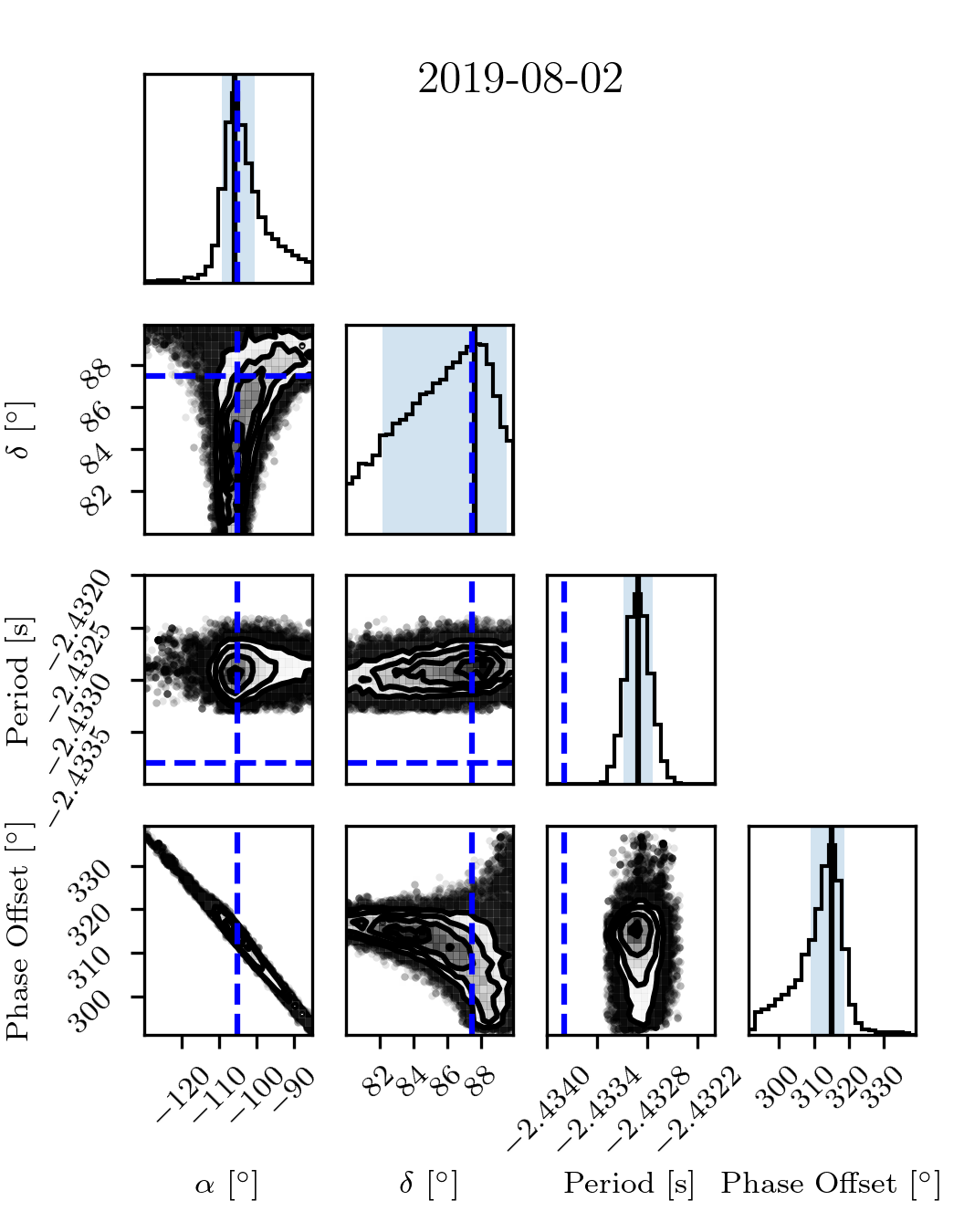
We implemented an MCMC sampler using emcee (Foreman-Mackey et al., 2013) to explore the posterior distribution of these parameters. An example set of prior distributions are listed in Table 2, and the empirical estimates with uncertainties reflecting residuals and RMS errors from Kucharski et al. (2016) are taken into consideration for the specific search band for that observation. Specifically, the empirical uncertainties are approximately $\alpha_{\sigma}\sim 14^{\circ}$ , $\delta_{\sigma}\sim 0.5^{\circ}$ , and $P_{\sigma}\sim 0.412\times 10^{-3}$ s. An initial exploration was performed using wider search bands for each parameter, but the uncertainties of the fit were characterised across search bands similar to those referenced in Table 2.

Each MCMC production run consisted of 5000 steps, with the first 1000 steps discarded as burn-in. The best-fit parameters and their uncertainties were estimated using the mode and full width half maximum (FWHM) of the posterior distributions. The corresponding corner plots from each run are shown in Figure 11 and are generated using corner (Foreman-Mackey, 2016).

4 Results

Table 3: Best estimates of parameters and their uncertainties derived from post burn-in MCMC samples. The estimate and asymmetric errors are derived from taking the mode and FWHM of the sample distributions. The alpha (

\alpha

) and delta (

\delta

) of the empirical spin-pole (ICRF frame) and period calculated at time of observation are given and we note the spin-axis,

\hat{\Psi}_{\text{emp}}(\alpha_{\text{emp}},\delta_{\text{emp}})

is inverted as this forms a right hand coordinate system such to complete the reference frame transforms, consistent with Koshkin et al. (2017). In this convention, the spin-pole of Ajisai is pointing toward the north celestial pole and whilst the absolute value for the rotation period is given, the spin-direction would be counter-clockwise.

Night Observed	$\alpha$ [^∘]	$\delta$ [^∘]	$\|P\|$ [s]	$\alpha_{\text{emp}}$ [^∘]	$\delta_{\text{emp}}$ [^∘]	$P_{\text{emp}}$ [s]
2019-08-01	$-102.40\,^{+21.81}_{-10.01}$	$87.65\,^{+0.53}_{-1.49}$	$2.4326\,^{+0.00009}_{-0.00009}$	$-103.67$	$87.39$	2.4337
2019-08-02	$-105.89\,^{+5.40}_{-3.42}$	$87.59\,^{+1.93}_{-5.43}$	$2.4329\,^{+0.00017}_{-0.00017}$	$-105.0$	$87.46$	2.4338
2019-08-07	$-111.19\,^{+21.39}_{-7.77}$	$87.49\,^{+1.61}_{-2.87}$	$2.4333\,^{+0.00067}_{-0.00095}$	$-111.8$	$87.84$	2.4343
2019-08-16	$-120.94\,^{+20.81}_{-6.77}$	$88.60\,^{+0.46}_{-0.51}$	$2.4352\,^{+0.00011}_{-0.00007}$	$-122.9$	$88.60$	2.4352

Figure 12 displays the brightness maps created from the best fit MCMC parameters. The arrangement of mirrors into triplets is clearly seen across varying latitudes in the body fixed frame and the brightest regions of the surface reflectivity align well with the expected mirror positions. Table 3 displays the best estimates and errors calculated from taking the mode and FWHM of the sample distributions.

It should also be noted that for the purpose of creating a right-handed coordinate system, our spin-axis results would be inverted to represent the true orientation of Ajisai i.e. pointing towards the south celestial pole as opposed to the north.

Figure 13 displays the residual measurements between the MCMC estimate and the empirically predicted values with the errors combined in quadrature. It is clear that the spin-pole estimations are close to the empirical value predictions and the first and fourth observation are particularly well constrained. The spin-pole $\delta$ residual for the second observation is not well constrained, however this is expected due to this observation covering fewer mirrors.

The empirical model provides a prediction of only the long-term, secular evolution of the spin period; it does not account for short-term variations, which could be driven—at least in part—by factors such as changes in solar illumination (Koshkin et al., 2017) and asymmetry in the surface reflectivity introduced by the launch adapter ring and polar cap (Hattori and Otsubo, 2019). We find that only the 2019-08-16 observation agrees with the empirical model, but all four lie within the interval (-0.8 to 1.2 ms) reported by Koshkin et al. (2017).

It is also worthwhile to mention that the relative motion between the observer and the target affects the measured apparent spin period regardless of the chosen reference frame—be it Earth-Centered Inertial (e.g., ICRF), Earth-Centered Earth-Fixed (e.g., ITRF), or the satellite’s body frame. We determine the rotation period by forward-modelling the ICRF phase-angle bisector into the body frame and maximizing its alignment with a static body-fixed mirror map; the fitted P is therefore the sidereal spin period, with observer/Sun relative motion handled inside the model rather than corrected afterwards. In contrast, Calatroni et al. (2025), first measure an apparent (synodic) period from inter-flash spacings within a triplet ("four-flash method"), and then apply a geometric correction to obtain the sidereal period.

5 Summary

We have demonstrated the feasibility of determining the spin-state of the Ajisai satellite through high-cadence photometric observations obtained using the SuperWASP instrument. We analysed four observations in August 2019, capturing sub-second glints consistent with specular reflections off Ajisai’s mirrors. By transforming TLE-derived vectors from the ICRF into the satellite’s body-fixed frame and generating latitude-longitude brightness maps, we showcase a novel method for mapping surface reflectivity.

Our methodology combines precision light curve extraction from streaked images with an MCMC-driven fitting process that aligns brightness maps in the satellite’s body-fixed frame with modelled mirror positions. This indicates that constrained spin-state estimations can be derived from high-cadence photometry without relying on complex BRDF modelling or detailed prior knowledge of the satellite’s shape which is consistent with earlier photometric studies of Ajisai. The spin-state of a satellite significantly influences the morphology of light curves, governing the periodicity and modulation patterns that can be further exploited using machine learning models such as boosted decision trees (Shrive et al., 2024).

Our best-fit spin-state solutions are consistent with empirical model predictions and observed variations in spin-period, affirming the adequacy of our mirror models in capturing the satellite’s reflective behaviour. Notably, these results were achieved using relatively modest ground-based hardware adapted for high temporal resolution.

The original SuperWASP instrument used in this study has since been upgraded to STING, a wide-field multi-colour system that began routine operations in 2023 (Airey et al., 2025). This newer system, with reduced read noise (due to CMOS over CCD) and four distinct bandpasses, offers enhanced capabilities for resolving short-timescale glints with higher precision. In the case of Ajisai and similar objects, this will improve spin-state extraction and enable better resolution of closely separated objects during Rendezvous and Proximity Operations (RPO) or Active Debris Removal (ADR) missions.

These results affirm the value of high-cadence optical photometry for SDA applications, particularly for characterising the attitude of tumbling or rapidly spinning LEO objects—a critical capability in an increasingly congested orbital environment.

Acknowledgements

This work makes use of data from the original SuperWASP instrument operated on the island of La Palma by the University of Warwick in the Spanish Observatory del Roque de los Muchachos of the Instituto de Astrofísica de Canarias. JAB acknowledges support from the Science and Technology Facilities Council (grant ST/Y50998X/1). We thank Nikolay Koshkin at the Odessa National University for sharing their measurements of the Ajisai mirror positions. For the purpose of open access, the author has applied a Creative Commons Attribution (CC-BY) licence to any Author Accepted Manuscript version arising from this submission.

The authors would like to thank the reviewers for their comments and suggestions that helped to improve the quality of the final manuscript.

Conflict of Interest

Authors declare no conflict of interest.

Data Availability

The data underlying this article will be shared on reasonable request to the corresponding author.

References

R. J.S. Airey, P. Chote, J. A. Blake, B. F. Cooke, J. McCormac, P. Allen, A. MacManus, D. Pollacco, B. Shrive, and R. West (2025) A comprehensive survey of the geo-belt using simultaneous four-colour observations with sting. Advances in Space Research 75 (7), pp. 5757–5780. External Links: ISSN 0273-1177, Document, Link Cited by: §5.
G. Arfken and A. A. Mullin (1967) Mathematical Methods for Physicists. American Journal of Physics 35 (11), pp. 1097–1098. External Links: Document Cited by: §3.1.
G. P. Badura and C. R. Valenta (2024) Physics-Guided Machine Learning for Satellite Spin Property Estimation from Light Curves. Journal of the Astronautical Sciences 71 (5), pp. 41. External Links: Document Cited by: §1.
A. Becker (2015) HOTPANTS: High Order Transform of PSF ANd Template Subtraction. Note: Astrophysics Source Code Library External Links: 1504.004 Cited by: §2.1.
J. A. Blake, P. Chote, D. Pollacco, W. Feline, G. Privett, A. Ash, S. Eves, A. Greenwood, N. Harwood, T. R. Marsh, D. Veras, and C. Watson (2021) DebrisWatch I: A survey of faint geosynchronous debris. Advances in Space Research 67 (1), pp. 360–370. External Links: Document Cited by: §1.
J. A. Blake (2022) Looking out for a sustainable space. Astronomy & Geophysics 63 (2), pp. 2.14–2.20. Cited by: §1.
A. Boonrath, T. Singh, and E. M. Botta (2024) Identification of parameters for tethered satellite system to emulate net-captured debris towing. Acta Astronautica 225, pp. 676–688. External Links: Document Cited by: §1.
C. Calatroni, G. Métris, C. Courde, D. Phung, J. Chabé, M. Aimar, N. Maurice, and H. Mariey (2025) A new model to predict ajisai satellite reflected sunlight flashes and application to the determination of its rotation parameters.. Advances in Space Research. External Links: ISSN 0273-1177, Document, Link Cited by: §1, §2.2, §4.
P. Chote, D. J. Sullivan, R. Brown, S. T. Harrold, D. E. Winget, and D. W. Chandler (2014) Puoko-nui: a flexible high-speed photometric system. Monthly Notices of the Royal Astronomical Society. Cited by: §2.
P. Chote, J. Blake, and D. Pollacco (2019) Precision Optical Light Curves of LEO and GEO Objects. In Advanced Maui Optical and Space Surveillance Technologies Conference, pp. 52. Cited by: Figure 5, Figure 5, §2.1.
Y. Endo, H. Kojima, and P. M. Trivailo (2022) New formulation for evaluating status of space debris capture using tether-net. Advances in Space Research 70 (10), pp. 2976–3002. External Links: Document Cited by: §1.
eoPortal – Earth Observation Portal (2012) EGS (experimental geodetic satellite) / ajisai. Note: https://www.eoportal.org/satellite-missions/egs#spacecraftAccessed: 2025-07-05 Cited by: §1.1.
D. Foreman-Mackey, D. W. Hogg, D. Lang, and J. Goodman (2013) emcee: The MCMC Hammer. PASP 125 (925), pp. 306. External Links: Document, 1202.3665 Cited by: §3.3.
D. Foreman-Mackey (2016) Corner.py: scatterplot matrices in python. The Journal of Open Source Software 1 (2), pp. 24. External Links: Document, Link Cited by: §3.3.
A. Gelman, J. B. Carlin, H. S. Stern, D. B. Dunson, A. Vehtari, and D. B. Rubin (2013) Bayesian data analysis. Third edition, Chapman & Hall/CRC Texts in Statistical Science Series, CRC, Boca Raton, Florida. External Links: ISBN 9781439840955 1439840954, Link Cited by: Table 2, Table 2.
H. Goldstein (1980) Classical mechanics. Second edition. Note: First edition published in 1967. Cited by: §3.1.
D. Hall, J. Africano, D. Archambeault, B. Birge, D. Witte, and P. Kervin (2006) AMOS Observations of NASA’s IMAGE Satellite. In The Advanced Maui Optical and Space Surveillance Technologies Conference, S. Ryan (Ed.), pp. E76. Cited by: §1.
D. Hall and P. Kervin (2013) Analysis of Faint Glints from Stabilized GEO Satellites. In Advanced Maui Optical and Space Surveillance Technologies Conference, S. Ryan (Ed.), pp. E34. Cited by: §3.1.
B. Hapke (2012) Theory of Reflectance and Emittance Spectroscopy. External Links: Document Cited by: §1.
A. Hattori and T. Otsubo (2019) Time-varying solar radiation pressure on Ajisai in comparison with LAGEOS satellites. Advances in Space Research 63 (1), pp. 63–72. External Links: Document Cited by: §4.
G. Kirchner, W. Hausleitner, and E. Cristea (2007) Ajisai spin parameter determination using graz kilohertz satellite laser ranging data. Geoscience and Remote Sensing, IEEE Transactions on 45, pp. 201 – 205. External Links: Document Cited by: §1.1.
N. Koshkin, L. Shakun, N. Burlak, E. Korobeynikova, S. Strakhova, S. Melikyants, S. Terpan, and A. Ryabov (2017) Ajisai spin-axis precession and rotation-period variations from photometric observations. Advances in Space Research 60 (7), pp. 1389–1399. External Links: Document Cited by: Appendix A, §1, Figure 10, Figure 10, Figure 12, Figure 12, §3.2, §3.3, Figure 13, Figure 13, Table 3, Table 3, §4.
N. Koshkin, L. Shakun, E. Korobeynikova, S. Melikyants, S. Strakhova, V. Dragomiretsky, A. Ryabov, S. Terpan, and T. Golubovskaya (2024) Determination of the spacecraft’s spin axis orientation. Photometric patterns method. Advances in Space Research 74 (11), pp. 5725–5744. External Links: Document Cited by: §1.
D. Kucharski, G. Kirchner, S. K. Flegel, M. K. Jah, and J. C. Bennett (2019a) High-Definition Photometry — An Optical Method for Remote Detection of MMOD Impacts on Satellites. In First International Orbital Debris Conference, LPI Contributions, Vol. 2109, pp. 6075. Cited by: §1.
D. Kucharski, G. Kirchner, T. Otsubo, S. K. Flegel, H. Kunimori, M. K. Jah, F. Koidl, J. C. Bennett, M. Steindorfer, and P. Wang (2020) Quanta Photogrammetry of Experimental Geodetic Satellite for remote detection of micrometeoroid and orbital debris impacts. Acta Astronautica 174, pp. 24–31. External Links: Document Cited by: §1.
D. Kucharski, G. Kirchner, T. Otsubo, H. Kunimori, M. K. Jah, F. Koidl, J. C. Bennett, H. Lim, P. Wang, M. Steindorfer, and K. Sośnica (2019b) Hypertemporal photometric measurement of spaceborne mirrors specular reflectivity for Laser Time Transfer link model. Advances in Space Research 64 (4), pp. 957–963. External Links: Document Cited by: §1.1, §1.
D. Kucharski, G. Kirchner, T. Otsubo, H. Lim, J. Bennett, F. Koidl, Y. Kim, and J. Hwang (2016) Confirmation of gravitationally induced attitude drift of spinning satellite Ajisai with Graz high repetition rate SLR data. Advances in Space Research 57 (4), pp. 983–990. External Links: Document Cited by: Appendix A, Figure 2, Figure 2, §1.1, §1, Figure 11, Figure 11, §3.3.
D. J. B. Laurence (2022) Attitude characterisation of space objects using optical light curves. Ph.D. Thesis, University of Southampton, University of Southampton. External Links: Link Cited by: §1.
J. McDowell (2002) The united nations registry of space objects - notes. Note: http://planet4589.org/space/un/un_notes.htmlAccessed: 2025-06-29 Cited by: §1.1.
T. Meyer, D. Keil, D. Traub, S. Scharring, W. Riede, T. Dekorsy, M. Nussbaum, M. Lengowski, R. Schweigert, and S. Klinkner (2024) High-Fidelity Light Curve Simulation and Validation Using Empirical Data. In Advanced Maui Optical and Space Surveillance (AMOS) Technologies Conference, S. Ryan (Ed.), pp. 115. Cited by: §1.
T. Otsubo, J. Amagai, H. Kunimori, and M. Elphick (2000) Spin motion of the AJISAI satellite derived from spectral analysis of laser ranging data. IEEE Transactions on Geoscience and Remote Sensing 38 (3), pp. 1417–1424. External Links: Document Cited by: Figure 1, Figure 1.
D. L. Pollacco, I. Skillen, A. Collier Cameron, D. J. Christian, C. Hellier, J. Irwin, T. A. Lister, R. A. Street, R. G. West, D. R. Anderson, W. I. Clarkson, H. Deeg, B. Enoch, A. Evans, A. Fitzsimmons, C. A. Haswell, S. Hodgkin, K. Horne, S. R. Kane, F. P. Keenan, P. F. L. Maxted, A. J. Norton, J. Osborne, N. R. Parley, R. S. I. Ryans, B. Smalley, P. J. Wheatley, and D. M. Wilson (2006) The WASP Project and the SuperWASP Cameras. Publications of the Astronomical Society of the Pacific 118, pp. 1407–1418. External Links: astro-ph/0608454, Document Cited by: §2.1, §2.
B. Rhodes (2019) Skyfield: High precision research-grade positions for planets and Earth satellites generator. Note: Astrophysics Source Code Library, record ascl:1907.024 External Links: 1907.024 Cited by: §3.1.
A. Rossi, N. Sánchez-Ortiz, E. David, R. Opromolla, and D. Grishko (2024) Future activities in the near-earth space in the face of ever-increasing space traffic. Acta Astronautica 225, pp. 891–897. External Links: Document Cited by: §1.
S. Sampath and J. Feng (2024) Intelligent and robust control of space manipulator for sustainable removal of space debris. Acta Astronautica 220, pp. 108–117. External Links: Document Cited by: §1.
M. Sasaki and H. Hashimoto (1987) Launch and Observation Program of the Experimental Geodetic Satellite of Japan. IEEE Transactions on Geoscience and Remote Sensing 25 (5), pp. 526–533. External Links: Document Cited by: §1.1, §1.1.
G. Seeber (2003) Satellite geodesy. De Gruyter, Berlin, New York. External Links: Link, Document, ISBN 9783110200089 Cited by: §3.1.
J. Serrano, A. Gallego, Á. Martínez, and D. Moreno (2024) Monitoring of Rendezvous & Proximity Operations With SST and SDA Techniques Combination. In Advanced Maui Optical and Space Surveillance (AMOS) Technologies Conference, S. Ryan (Ed.), pp. 134. Cited by: §1.
B. Shrive, D. Pollacco, P. Chote, J. A. Blake, B. F. Cooke, J. McCormac, R. West, R. Airey, A. MacManus, and P. Allen (2024) Classifying LEO satellite platforms with boosted decision trees. RAS Techniques and Instruments 3 (1), pp. 247–256. External Links: Document Cited by: §5.
J. Šilha, J. Pittet, M. Hamara, and T. Schildknecht (2018) Apparent rotation properties of space debris extracted from photometric measurements. Advances in Space Research 61 (3), pp. 844–861. External Links: Document Cited by: §1.
R. W. Sinnott (1984) Virtues of the Haversine. Sky Telesc. 68, pp. 159. Cited by: Appendix B.
S. Zhao, M. Steindorfer, G. Kirchner, Y. Zheng, F. Koidl, P. Wang, W. Shang, J. Zhang, and T. Li (2020) Attitude analysis of space debris using SLR and light curve data measured with single-photon detector. Advances in Space Research 65 (5), pp. 1518–1527. External Links: Document Cited by: §1.

Appendix A Empirical Model Calculations

Spin-Axis Evolution

The orientation of the Ajisai spin axis can be expressed by a set of time-dependent equations, following the empirical model developed by Kucharski et al. (2016). The coordinates of a vector oriented at the azimuthal angle $\phi$ about the concentric cone of radius $R$ , and with its axis at right ascension $\alpha$ and declination $\delta$ , are defined by the transformation:

S=R_{3}(-\alpha)\,R_{2}(\delta-90^{\circ})\,R_{3}(-\phi)\,R_{2}(-R),

(11)

where $R_{3}$ and $R_{2}$ are the rotation matrices about the $z$ - and $y$ -axes, respectively, as defined in Equations 2 and 3.

The inertial orientation of the nutation cone axis $\vec{v}_{N}$ is calculated as:

\vec{v}_{N}=S\cdot\vec{z},\quad\text{with }\vec{z}=[0,0,1]

(12)

The parameters for the matrix $S$ describing the precession cone are:

1.

Right ascension of the cone axis: $\alpha=88.90^{\circ}$
2.

Declination of the cone axis: $\delta=-88.85^{\circ}$
3.

Radius of the precession cone: $R=1.08^{\circ}$ ]
4.

Precession angle (azimuth): $\phi=-0.0277404\,D+452.803^{\circ}$

where $D$ is the number of days since launch (MJD 46654.86).

The spin axis vector $\vec{v}_{S}$ is calculated using a time-varying nutation cone defined about $\vec{v}_{N}$ , with parameters:

1.

Nutation cone radius:

$R=7.66693\times 10^{-9}\,D^{2}-0.0000656721\,D+1.42878^{\circ},$
2.

Nutation angle (azimuth):

$\phi=8.08453575\times 10^{-7}\,D^{2}+3.07506\,D-19238.5^{\circ}.$

Using these parameters, the transformation matrix $S$ is recomputed with the updated $\alpha$ and $\delta$ (from $\vec{v}_{N}$ ), and the spin axis vector is given by:

\vec{v}_{S}=S\cdot\vec{z}.

(13)

Spin Period Evolution

The spin period $P$ , of Ajisai is modelled as an exponential trend function (Koshkin et al., 2017) :

P(D)=1.4934\cdot\exp(0.000040553\cdot D)\,\text{[s]},

(14)

which describes the gradual loss of rotational energy due to weak magnetic torque effects.

Appendix B Separation Calculation

Our calculation of the quantity $sep(x_{i},\,y_{j})$ is calculated using the Haversine formula for small distances (Sinnott, 1984). These are described by Equations 15 and 16 respectively. The subscripts of $\lambda$ and $\phi$ denote the longitude and latitude components of $x_{i}$ and $y_{j}$ respectively.

\begin{split}A(x_{i},y_{j})&=\sin^{2}\!\left(\frac{(y_{j})_{\phi}-(x_{i})_{\phi}}{2}\right)\\ &\quad+\cos\!\big((x_{i})_{\phi}\big)\,\cos\!\big((y_{j})_{\phi}\big)\,\sin^{2}\!\left(\frac{(y_{j})_{\lambda}-(x_{i})_{\lambda}}{2}\right)\end{split}

(15)

sep(x_{i},\,y_{j})=2\,\arctan 2\!\left(\sqrt{A(x_{i},\,y_{j})},\sqrt{1-A(x_{i},\,y_{j})}\right)

(16)

\bsp