An Adaptive Proximal Point Method for Nonsmooth and Nonconvex Optimization on Hadamard Manifolds
Abstract
This paper addresses a class of nonsmooth and nonconvex optimization problems defined on complete Riemannian manifolds. The objective function has a composite structure, combining convex, differentiable, and lower semicontinuous terms, thereby generalizing the classical framework of difference-of-convex programming. Motivated by recent advances in proximal point methods in Euclidean and Riemannian settings, we propose two variants: one that uses the Lipschitz constant of the gradient of the smooth part, suitable when this parameter is accessible, and another that dispenses with such knowledge, expanding its applicability. We analyze the complexity of both approaches, establish their convergence, and illustrate their effectiveness through numerical experiments.
Keywords: Riemannian manifolds; Nonconvex optimization; Nonsmooth optimization; Composite minimization
MSC 2020: 90C30; 90C26; 49Q99
1 Introduction
In this paper, we study a class of nonsmooth and nonconvex optimization problems defined on a complete Riemannian, called in this introduction of NNOP-CR. The objective function has a composite structure, where one term is convex, another term is continuously differentiable with a Lipschitz continuous gradient, and a third term is proper and lower semicontinuous but not necessarily convex. When the sum of the nonsmooth and the differentiable terms is assumed to be convex, the problem reduces to the well-known framework of difference-of-convex (DC) programming, which has been widely investigated in the literature. However, by allowing the nonsmooth component to be nonconvex, we obtain a broader and more challenging class of problems that generalizes the classical DC setting. Such formulations naturally arise in many areas of applied mathematics and engineering. Examples include machine learning [7], image processing image processing [7], compressed sensing [47], location optimization [34], biochemistry modeling [7], sparse optimization [29], clustering methods [aragón2020boosted, 12], hierarchical clustering [35], clusterwise linear regression [11], multicast network design [28], and multidimensional scaling [3].
We now focus our discussion on the efficient methods applied for solving problems belonging to NNOP-CR in the Euclidian context. A popular and probably the first algorithm developed to solve DC problems was the Difference of Convex Algorithm (DCA), see [41, 42]. A significant progress in this field was the development of the Boosted DC Algorithm (BDCA) [6, aragón2020boosted, 8], which enhances the convergence speed of the traditional DCA through the integration of a line search strategy; see also [7, 48] for other recent contributions. This strategy enables larger step sizes compared to the standard DCA, leading to improved convergence efficiency and better solution quality by avoiding suboptimal local minima. The initial BDCA was mainly designed for scenarios where the first DC component is differentiable, ensuring a descent direction. However, its original formulation has limitations when both components are nondifferentiable.
To overcome the challenge that BDCA encounters as mentioned in the previous paragraph, the recent work [27] introduced the nonmonotone Boosted Difference of Convex Algorithm (nmBDCA). The key difference between nmBDCA and BDCA arises when the first component is nondifferentiable. In such situations, the line search direction utilized in BDCA may not guarantee a descent direction, rendering the standard Armijo line search ineffective. To address this issue, nmBDCA incorporates a nonmonotone Armijo-like line search that remains effective even when the first component is not differentiable. This adjustment enables nmBDCA to tackle a wider range of problems, thereby broadening its applicability beyond BDCA and improving the efficiency of the line search. Further developments beyond BDCA and nmBDCA were recently explored in [26], where the subproblem at each iteration of its inexact nmBDCA is solved approximately using a relative error tolerance.
We now discuss on the recent developments on Riemannian DC problems. The crescent interest in optimization methods on Riemannian manifolds is due to the fact that practical applications arise whenever the natural structure of the data is modeled as an optimization problem on a Riemannian manifold. For instance see [10, 18, 19, 21, 24, 29, 38, 46, 49]. As far as we know, the study presented in [40] was the first to address DC functions within Riemannian manifolds. Specifically, the authors in [40] introduced the proximal point algorithm for DC functions and analyzed its convergence in the context of Hadamard manifolds. More recently, [1] proposed a refined version of the algorithm in [40] in the same Riemannian framework, aiming to enhance the convergence speed of the method introduced in [40]. In the recent paper [29], a DC algorithm is presented for sparse optimization problems having a cardinality or rank constraint. The main idea in [29] is to transform the cardinality-constrained problem into a penalty function form and derive exact penalty parameter values for some optimization problems, especially for quadratic minimization problems which often appear in practice. Thus, the new problem belongs to NNOP-CR, i.e., a DC problem with three nonlinear functions. More relevant researches about the proximal point methods within the framework of Riemannian manifolds can be found in [5, 15, 14, 23, 25, 16, 32, 44] and in [1, 13, 22, 36, 37, 40].
In the case where the Riemannian manifold is the Euclidian space, in [4] is proposed a PPM to solve a problem in NNOP-CR, under the same conditions as mentioned before. The method proposed in [4] is based on a proximal-point framework. At each iteration, it solves a strongly convex subproblem that involves both the nonsmooth and smooth components of the objective. The construction of these subproblems requires knowledge of the Lipschitz constant associated with the gradient of the differentiable term. Similarly, in [2] the authors proposed an algorithm based on a proximal gradient method for a particular case by assuming that the smooth function has a gradient Hölder.
In this paper, we present two variants for the proximal point methods for solving NNOP-CR. In our convergence analysis, we require that only one of the functions is convex. In the first method, prior knowledge of the Lipschitz constant associated to the gradient of the smooth part is required, making it more suitable for problems in which this constant is easy to compute. However, determining such a constant is not always straightforward. Therefore, in this paper, we propose a second method that does not require prior knowledge of the Lipschitz constant. We analyze the complexity of both methods and prove that they reach an approximate solution in a finite number of iterations, with complexity of order , with to be specified later.
The remainder of this paper is organized as follows. In Section 2, we present preliminary results to support the development of the proposed methods. Section 3 introduces the first version of the Riemannian proximal point method and demonstrates its effectiveness. In Section 4, we propose a second version of the method, which does not require prior knowledge of the Lipschitz constant, and analyze its worst-case iteration complexity. Section 5 is devoted to the convergence analysis under the assumption that the objective function satisfies the Kurdyka-Łojasiewicz (KL) property. In Section 6, we illustrate the applicability of the proposed methods by provideing numerical experiments. Finally, Section 7 presents the conclusions of the paper.
2 Preliminaries
Throughout this work, will denote a finite-dimensional Riemannian manifold, and will represent the tangent space of at the point . The norm induced by the Riemannian metric will be denoted by .
By definition, a Hadamard manifold is a complete, simply connected Riemannian manifold with nonpositive sectional curvature. In this work, we restrict our analysis to manifolds of this type.
The Riemannian metric provides the following fundamental notions:
-
(i)
Let be a piecewise smooth curve with and . Its length is given by
-
(ii)
The Riemannian distance between and is defined by
where the infimum is taken over all such curves. This distance induces the topology of .
-
(iii)
Given a geodesic joining to , the parallel transport along is denoted by .
-
(iv)
A vector field along is parallel if . In particular, is a geodesic when its velocity field is parallel.
-
(v)
For any , the parallel transport is an isometry.
The completeness of the Hadamard manifold allows the definition of the exponential map
for all . Consequently, the inverse is smooth (). Since , the function is , and its gradient at , , is given by as shown in [25, Proposition 3.3].
A classical result on Hadamard manifolds is the “Comparison Theorem” for geodesic triangles (see [39, Proposition 4.5]), which states that, for any ,
| (1) |
Let . Its domain is defined as
We say that is proper if , and that it is lower semicontinuous (lsc) at if
The Fréchet subdifferential of at is defined as
where is given by
The limiting subdifferential of at is defined as
where
It holds that . Moreover, if is differentiable at , then
Finally, if attains a local minimum at , then .
In the convex case, we also recall some classical results of convex analysis. Given a convex function , the subdifferential of at is defined by
In this case, for every it holds that
These definitions lead to several fundamental properties, which we summarize below.
-
(a)
for every the set is nonempty, convex, and compact. See [43, Theorems 4.5–4.6].
-
(b)
consider a sequence . If for all , then the sequence is bounded and every accumulation point of belongs to .
-
(c)
Let , where is proper and lsc, and is continuously differentiable in a neighborhood of . Then
For more details, see [31, Theorem 4.13]. The next result is fundamental for the definition of critical points. Its proof can be found in [30, Theorem 5.2].
Theorem 2.1.
If is a local minimizer of Problem (5), then
| (2) |
A point that satisfies (2) is called a stationary point of Problem (5). Since this condition may be difficult to verify, one usually adopts the relaxed condition
| (3) |
in which case is referred to as a critical point of . We denote by the set of all critical points of and assume, throughout this work, that .
Proposition 2.2.
Let be a differentiable function whose gradient mapping is Lipschitz continuous with constant . Then, for every and ,
| (4) |
Proof.
See [14, Lemma 2.1]. ∎
3 The First Riemannian Proximal Point Method
In this section, we present the first Riemannian proximal point method (R-PPM) for solving the following problem:
| (5) |
where is a complete Riemannian manifold, is a convex function, is a continuously differentiable function with its gradient being Lipschitz continuous over , and is a proper and lower semicontinuous function.
Throughout it, we assume the following assumptions.
-
(A1)
For each fixed and some , we have that
-
(A2)
Function is bounded from below, i.e., there exists such that for every .
We note that if is bounded from below or convex, Assumption (A1) is satisfied. Next, we formally describe R-PPM.
Algorithm R-PPM
-
Step 0. Given , a sequence of positive numbers such that and set
-
Step 1. Calculate
(6) -
Step 2. Compute
(7) -
Step 3. If , stop. Otherwise, set and return to Step 1.
We now make some remarks about R-PPM. First, we assume that the Lipschitz constant satisfying (4) can be computed, that is, we suppose that is known. Second, the real sequence in Step 0 can be any nondecreasing sequence belonging to the interval . Third, after finding , and as in (6), for a given starting point the next point is generated by solving the Subproblem (7), which we assume to be easy to solve.
Note that when , R-PPM becomes exactly the algorithm DCPPA proposed in [40], even so, our problem is more general, as we consider that only the function is convex.
We establish some preliminaries results about the sequence generated by R-PPM. First, we prove that the sequence is well-defined, along with proposing a practical stopping criterion for R-PPM.
Proposition 3.1.
Let be the sequence generated by R-PPM. Then, the following statements hold:
-
(a)
is well-defined;
-
(b)
If , then R-PPM stops at a solution of (5).
Proof.
Let be the input for R-PPM. For some we assume that R-PPM reached the iteration , and we will show that the -th iterate exists. Since is differentiable and is convex, the well definition of the sequence in (6) follows directly from the fact that is a complete Hadamard manifold. Now, note that the assumptions that is proper and lsc imply that defined in (7), is proper and lsc as well. Furthermore, Assumption (A1) implies that if is large enough, then we obtain that , for some and As a consequence, we use (7) to conclude that
Thus, since we can conclude that is coercive. As a result, we can conclude that the function has minimizers and we will denote one of them by , where . Hence, from any the R-PPM generates
From now on, we assume that for all otherwise, Proposition 3.1(b) ensures that R-PPM stops at a solution of Problem (5).
Proposition 3.2.
The sequence generated by R-PPM satisfies
Proof.
We first observe that (7) implies that for each and In particular, for , we have
| (9) |
Due to the convexity of the function , the following inequality holds for each :
| (10) |
On the other hand, Proposition 2.2 with and yields
| (11) |
Thus, taking into account that inequalities (9), (10) and (11), imply that
| (12) | |||||
where Then, from (1) with and that
As a consequence,
| (13) |
Therefore, (12) and (13) imply that
from which the conclusion of the proof follows.
∎
As a consequence of the previous result, we next show that a sequence generated by R-PPM is monotonically decreasing.
Proposition 3.3.
Let be a sequence generated by R-PPM. Then,
-
(a)
The sequence is monotonically decreasing. As a consequence, it is convergent;
-
(b)
. In particular, as .
Proof.
It follows from Proposition 3.2 that
Since and , then we have for all Being bounded from below, see Assumption (A2), this implies that converges.
It follows from Proposition 3.2 and that
Summing up the previous inequality from to , we have
Letting goes to in the above inequality, taking in account Assumption (A2), we obtain the two conclusions. ∎∎
The next result shows that if there exists a cluster point of a sequence generated by R-PPM, then it is a critical point as defined in (3).
Theorem 3.4.
Let be a sequence generated by method R-PPM. Then, every cluster point of is a critical point of .
Proof.
Let be a cluster point of , and let be a subsequence of converging to . Then, it follows from (6) that there exist bounded subsequences and of and , respectively. Thus, we can suppose that (one can extract others subsequences if necessary).
Now, it follows from (7) that for all . In particular, for we obtain
From Proposition 3.3 (b) we have that As a consequence, we can guarantee that as . Since convergent, thus the previous inequality implies that Combining this with the assumption that is lower semicontinuous, we obtain that
The same argument as in (8) shows that there exists satisfying On the other hand and therefore, we have that
Thus, as , it follows from the property of limiting subdifferentials that . Therefore
This means that is a critical point of . Finishing the proof of the Theorem 3.4. ∎
The next theorem establishes an upper bound on the iteration complexity of the R-PPM method required to obtain an approximate solution with a prescribed tolerance.
Theorem 3.5.
Given , let be the sequence generated by R-PPM, for some . Then, the number of iterations such that
| (14) |
is bounded from above by
Proof.
We conclude this section with some remarks. Assume that the tolerance parameter satisfies , which is possible since is arbitrarily chosen in R-PPM. Then the following sequence is a valid example satisfying with :
| (16) |
where is a fixed parameter. Clearly, is nondecreasing, , and . Hence, if we choose as in (16), it follows from Theorem 3.5 that the complexity of R-PPM is
4 Adaptive R-PPM
As noted in the previous section, to implement R-PPM is necessary to know the constant , due to the condition for some given, see its Step 0. However, in practice, this constant may not be readily available or may require a greater effort to access it. To address this difficulty, we propose in this section a method similar to R-PPM but adaptive. That is, we do not need to know or any other constant that may be difficult to compute.
Lemma 4.1.
Let and be such that and
| (17) |
with Suppose that is a solution to the problem
| (18) |
and assume that
| (19) |
where is the Lipschitz constant to . Then,
| (20) |
Proof.
We first observe that the assumption that is convex implies that
with Since is -Lipschitz continuous, by assumption, we can apply Proposition 2.2 with and , combined with the assumption that , to conclude that
The two previous inequalities combined with the assumption that is a solution of Problem (18) yields
Using now that and the fact that in view of (17), the above inequality becomes to
| (21) |
On the other hand, the inequality (1) implies that
Thus, the previous inequality and (21) imply in
Since (19) holds, then we can conclude from the previous inequality that (20) holds, which concludes the proof. ∎
Taking into account the preivous result, we now state an adaptive proximal-point algorithm to solve the Problem (5).
Adap-RPPM
-
Step 0. Given an initial point and
-
Step 1. Given calculate
-
Step 1.2 Calculate
-
Step 2. Compute
-
Step 3. If , stop declaring that is a solution of (5). Otherwise, go to Step 4.
-
Step 4. If
(22) then , , and go to Step 1. Otherwise, , and go to Step 1.2.
We now make some remarks about Adap-RPPM. Initially, Adap-RPPM requires the parameters , , and , which are provided by the user and can be freely chosen. According to (22), small values of tend to produce larger decreases, which, hopefully, makes the method converge more quickly. It is important to emphasize that, for its execution, Adap-RPPM does not require prior knowledge of the constant from the Lipschitz condition of the gradient of , which makes the method advantageous in problems where this constant is unknown.
The well-defined Step of the Adap-RPPM is ensured, in particular, by item a) of Proposition 3.1. In turn, the well-defined Step follows directly from Lemma 4.1. Based on these results, we conclude that Adap-RPPM is well-defined.
Next, we demonstrate that the sequence generated by Adap-RPPM is bounded, a fundamental result to ensure the convergence of the method.
Lemma 4.2.
Suppose that is -Lipschitz continuous on Then, the sequence in Adap-RPPM satisfies
| (23) |
Proof.
By Lemma 4.1, we have that the decrease in Step 4 is satisfied whenever . Clearly, (23) is true if , since in this case does not need to be updated and will remain constant, equal to .
On the other hand, if and the parameter is updated so that there exists such that , then we have that . Since the parameter is not updated when it is greater than or equal to , we conclude that, starting from , the sequence of parameters remains constant and equal to .
Therefore, we can conclude that the sequence is bounded from above by . ∎
The following theorem establishes an iteration-complexity bound of for the proposed method.
Theorem 4.3.
Given , let be generated by the Adap-RPPM, such that
Then,
5 Under the Kurdyka-Lojasiewicz Property
In the context of descent algorithms applied to convex functions, one typically ensures global convergence, meaning that the entire sequence generated by the algorithm converges. However, when the objective functions lack convexity or quasiconvexity, the resulting sequences may display significant oscillations, and only partial convergence can generally be established. To address such challenges, the Kurdyka–Lojasiewicz (KL) property has emerged as a powerful analytical tool, especially in the study of asymptotic behavior of algorithms, such as the proximal point method.
Our main convergence result in this section is restricted to functions that satisfy the KL property, as stated below.
Definition 5.1.
A lower semicontinuous function satisfies the KL property at if there exist , a neighborhood of , and a continuous concave function with
-
(a)
;
-
(b)
is continuously differentiable on ;
-
(c)
on ;
-
(d)
For every with , we have
Next, we present an auxiliary result regarding the sequence generated by R-PPM. It is important to prove the main result in this section.
Lemma 5.1.
Let , , , and be sequences generated by R-PPM. Suppose that , for every , and that the function is differentiable with a continuous Lipschitz gradient with the associated constant . If has a cluster point then, for sufficiently larger, there exists such that
Proof.
We first observe that if , , , and are sequences generated by R-PPM, and , for every , then it follows from (6) that
Moreover, using the fact that , and are continuous, and the assumption that has a cluster point, we can conclude that has a cluster point, and hence that there exists such that, for sufficiently larger, there holds
Using these facts and simple algebraic manipulations we obtain that
which concludes the proof. ∎
In the following theorem, we establish sufficient conditions that guarantee the convergence of the sequence generated by the R-PPM. For this, we will consider that satisfies the KL property and that is -Lipschitz continuous.
Theorem 5.2.
Let be a sequence generated by R-PPM, and assume that , for every . Suppose that is -Lipschitz continuous and that has the KL property at any point . If the sequence has a cluster point , then the whole sequence converges to , which is a critical point of .
Proof.
Since has a cluster point , by assumption, we can select a subsequence that converges to . By Proposition 3.3 , without loss of generality, we can assume that for all , otherwise, there exists such that , i.e, the method stop after a finite number of steps. We have
| (25) |
where and in view of (6). Now, it follows from (7) that
| (26) |
Using now Lemma 5.1, (25) and (26), we obtain that
| (27) |
Let be such that , where is as in Definition 5.1. As , and for all , we can find a natural number , large enough, satisfying
and
| (28) |
where .
We now claim that for all , . To show the claim, we first show that whenever and for some , we have
| (29) |
Indeed, due to the property that is monotonically decreasing (see Proposition 3.2) and the assumption that on (see Definition 5.1(c)), we conclude from (27) that
As a consequence, we use the concavity of , and combine the previous inequality with ((d)), and (3.2) to conclude that
Hence,
where the last inequality holds since , for any positive real numbers and . As a consequence, (29) holds.
We now prove the claim by induction on . The claim is true for due to (28). We suppose that it also holds for , with , i.e., . Since , our choice of implies that for all . In particular, (29) can be applied for all . Thus, summing (29) from to , doing some algebraic manipulations and using the fact that , we obtain
| (30) |
As a consequence, we have
where the last two inequalities follows from (30) and (28), respectively. Thus, and for all . Using (30) we conclude that . Therefore, is a Cauchy sequence and, hence, is convergent. ∎
6 Application and Numerical Experiments
This section contains two subsections. The first presents a practical example of (5). The second is dedicated to numerical experiments.
6.1 A Practical Example of (5)
In this subsection, we show how the log-determinant optimization problem with constraints can be rewritten as in (5).
When is the indicator function of a convex set , (5) is equivalent to solving the following problem
| (31) |
In fact, (31) is equivalent to solving the following problem:
| (32) |
where , with being the indicator function defined as follows:
We now consider the following particular case of (31)
| (33) |
where the variable is , and the coefficients are , , and . This problem originates from a broad range of applications, particularly in network information theory and wireless communication; see [33, 45].
6.2 Numerical Experiments
In this subsection, we evaluate the numerical performance of the proposed Adap-RPPM method. We consider three illustrative minimization problems to assess the algorithm’s behavior in different scenarios. All experiments were conducted on a workstation equipped with a Xeon W3-2435 processor and 64 GB of RAM. The algorithms were implemented in Julia (version 1.11.5), using the Manopt toolbox [20] to solve the subproblem in (4) via the trust_regions solver. The stopping criterion was set to , with a maximum of 100 iterations. The complete source code used in the numerical experiments is freely available at https://github.com/mbortoloti/AdapRPPM.
6.2.1 Sensitivity to the Parameter
We first consider the minimization of
on , where , and are symmetric positive definite matrices. Here, denotes the trace of a matrix. In the DC decomposition we identify
The Riemannian gradient of is Lipschitz continuous with constant .
For the experiments, we set and (). The unique critical point of is
We initialized the algorithm with , where is the identity matrix. The tests were carried out with , , and , corresponding to . The method was executed until , with initial parameters .
Figure 1 shows the evolution of as a function of the iteration count. The results confirm that strongly influences the convergence speed. For , convergence is reached in 42 iterations, while for the method requires 56 iterations. The slowest case occurs with , where 93 iterations are needed. This behavior can be explained by the role of in controlling the step size: very small values make the initial steps overly conservative, while yields more aggressive yet stable steps. Note that the sequence remains constant throughout the iterations.

| 0.8192 | 1.024 | 0.64 | 0.8 | 1.0 | |
| Iterations | 56 | 48 | 93 | 58 | 42 |
6.2.2 Scalability with Manifold Dimension
We next analyze Adap-RPPM for the function defined by
Its critical points satisfy .
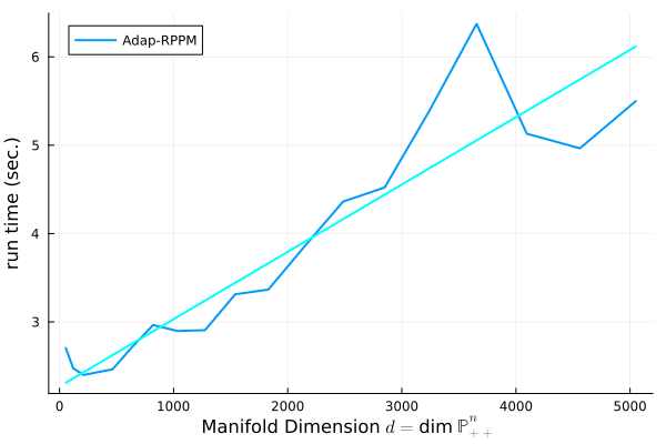
The experiments were conducted with matrix sizes , corresponding to manifold dimensions ranging from 55 to 5050. The initialization was set to for each , with . Figure 2 illustrates the computational cost, revealing a remarkably weak dependence of CPU time on the manifold dimension. The observed growth rate, benchmarked against a reference slope of , highlights the scalability of the proposed method in high-dimensional settings.
6.3 Comparison with Baseline Methods
Finally, we consider the minimization of
defined on . In this case, the decomposition is with and (so ). The critical points are all satisfying or .
We compared Adap-RPPM with two well-established algorithms: the Difference of Convex Algorithm (DCA) and the Difference of Convex Proximal Point Algorithm (DCPPA). Both methods were implemented in Manopt.jl [20], following their standard configurations. The benchmarking comprised 160 test cases across multiple dimensions, with 10 random initializations per dimension generated using rand(M) from the Manifolds.jl package [20].
Figure 3 presents the performance profiles of the three methods. The results indicate that Adap-RPPM consistently outperforms both DCA and DCPPA in terms of computational efficiency across all tested scenarios.

7 Conclusions
In this paper, we study variants of a generalized proximal point algorithm for minimizing compositions of functions combining convex, differentiable, and lower semicontinuous terms on Riemannian manifolds. We propose two approaches: the first based on knowledge of the Lipschitz constant of the gradient of the smooth part, and the second independent of this parameter, which expands its applicability in contexts where such information is unavailable.
Our theoretical results show that both variants are convergent and admit well-established complexity bounds, in line with recent literature. Numerical experiments demonstrate the practical effectiveness of the methods in problems with complex structures, reinforcing their relevance in the study of optimization on Riemannian manifolds.
In addition to contributing to advances in proximal methods on manifolds, this work suggests promising avenues for future research. Among these are the development of accelerated versions, analysis under more general assumptions, such as Hölder-type conditions, and the investigation of applications in other contexts.
Acknowledgements
This work was partially supported by the following grants from CNPq (National Council for Scientific and Technological Development) 401864/2022-7 .
References
- [1] (2020) A modified proximal point method for DC functions on Hadamard manifolds. Comput. Optim. Appl. 76, pp. 649–673. External Links: Document Cited by: §1.
- [2] (2024) On the complexity of a quadratic regularization algorithm for minimizing nonsmooth and nonconvex functions. Optimization Methods and Software, pp. 1–23. External Links: Document Cited by: §1.
- [3] (2001) D.c. programming approach to the multidimensional scaling problem. In From Local to Global Optimization, A. Migdalas, P. M. Pardalos, and P. Värbrand (Eds.), pp. 231–276. External Links: ISBN 978-1-4757-5284-7, Document, Link Cited by: §1.
- [4] (2017) Convergence analysis of a proximal point algorithm for minimizing differences of functions. Optimization 66 (1), pp. 129–147. External Links: Document Cited by: §1.
- [5] (2023) An inertial proximal point method for difference of maximal monotone vector fields in Hadamard manifolds. Journal of Global Optimization 85, pp. 941–968. External Links: Document Cited by: §1.
- [6] (2018) Accelerating the DC algorithm for smooth functions. Mathematical Programming 169, pp. 95–118. Cited by: §1.
- [7] (2025) Coderivative-based semi-Newton method in nonsmooth difference programming. Mathematical Programming 213, pp. 385–432. Cited by: §1, §1.
- [8] (2019) The boosted DC algorithm for linearly constrained DC programming. arXiv preprint arXiv:1908.01138. Cited by: §1.
- [9] (2005) Nonsmooth analysis and Hamilton–Jacobi equations on Riemannian manifolds. Journal of Functional Analysis 220 (2), pp. 304–361. Cited by: §2.
- [10] (2016) A second order nonsmooth variational model for restoring manifold-valued images. SIAM Journal on Scientific Computing 38 (1), pp. A567–A597. Cited by: §1.
- [11] (2018) Nonsmooth DC programming approach to clusterwise linear regression: optimality conditions and algorithms. Optimization Methods and Software 33 (1), pp. 194–219. Cited by: §1.
- [12] (2022) Solving a continuous multifacility location problem by DC algorithms. Optimization Methods and Software 37 (1), pp. 338–360. Cited by: §1.
- [13] (2016) Inexact proximal point methods for quasiconvex minimization on Hadamard manifolds. Journal of the Operational Research Society of China 4, pp. 397–424. External Links: Document Cited by: §1.
- [14] (2017) Iteration-complexity of gradient, subgradient and proximal point methods on Riemannian manifolds. Journal of Optimization Theory and Applications 173, pp. 548–562. Cited by: §1, §2.
- [15] (2010) Local convergence of the proximal point method for a special class of nonconvex functions on Hadamard manifolds. Nonlinear Analysis: Theory, Methods & Applications 73 (2), pp. 564–572. External Links: ISSN 0362-546X Cited by: §1.
- [16] (2015) Proximal point method for a special class of nonconvex functions on Hadamard manifolds. Optimization 64 (2), pp. 289–319. Cited by: §1.
- [17] (2018) Proximal point method for locally lipschitz functions in multiobjective optimization of Hadamard manifolds. Journal of Optimization Theory and Applications 179 (1), pp. 37–52. Cited by: §2.
- [18] (2024) The difference of convex algorithm on Hadamard manifolds. Journal of Optimization Theory and Applications 201 (1), pp. 221–251. Cited by: §1.
- [19] (2016) A parallel Douglas–Rachford algorithm for minimizing rof-like functionals on images with values in symmetric Hadamard manifolds. SIAM Journal on Imaging Sciences 9 (3), pp. 901–937. Cited by: §1.
- [20] (2022) Manopt.jl: optimization on manifolds in Julia. Journal of Open Source Software 7 (70), pp. 3866. External Links: Document Cited by: §6.2, §6.3.
- [21] (2008) Statistics on Riemannian manifolds: asymptotic distribution and curvature. Proceedings of the American Mathematical Society 136 (8), pp. 2959–2967. Cited by: §1.
- [22] (2020) A generalized proximal linearized algorithm for DC functions with application to the optimal size of the firm problem. Annals of Operations Research 289, pp. 313–339. Cited by: §1.
- [23] (2006) Convex and monotone-transformable mathematical programming problems and a proximal-like point method. Journal of Global Optimization 35, pp. 53–69. Cited by: §1.
- [24] (2019) Total variation regularization of pose signals with an application to 3D freehand ultrasound. IEEE Transactions on Medical Imaging 38 (10), pp. 2245–2258. Cited by: §1.
- [25] (2002) Proximal point algorithm on Riemannian manifolds. Optimization 51 (2), pp. 257–270. Cited by: §1, §2.
- [26] (2024) An inexact boosted difference of convex algorithm for nondifferentiable functions. arXiv preprint arXiv:2412.05697. Cited by: §1.
- [27] (2024) A boosted DC algorithm for non-differentiable dc components with non-monotone line search. Computational Optimization and Applications 88 (3), pp. 783–818. Cited by: §1.
- [28] (2018) A DC programming approach for solving multicast network design problems via the Nesterov smoothing technique. Journal of Global Optimization 72 (4), pp. 705–729. Cited by: §1.
- [29] (2018) DC formulations and algorithms for sparse optimization problems. Mathematical Programming 169, pp. 141–176. Cited by: §1, §1.
- [30] (2019) Nonconvex weak sharp minima on Riemannian manifolds. Journal of Optimization Theory and Applications 183 (1), pp. 85–104. Cited by: §2.
- [31] (2007) Nonsmooth analysis on smooth manifolds. Transactions of the American Mathematical Society 359 (8), pp. 3687–3732. Cited by: §2, §2.
- [32] (2009) Monotone vector fields and the proximal point algorithm on Hadamard manifolds. Journal of the London Mathematical Society 79. External Links: Link Cited by: §1.
- [33] (2007) An extremal inequality motivated by multiterminal information-theoretic problems. IEEE Transactions on Information Theory 53 (5), pp. 1839–1851. Cited by: §6.1.
- [34] (2014) An easy path to convex analysis and applications (vol. 14). Synthesis Lectures on Mathematics and Statistics Williston: Morgan & Claypool Publishers. Cited by: §1.
- [35] (2018) Nesterov’s smoothing technique and minimizing differences of convex functions for hierarchical clustering. Optimization Letters 12, pp. 455–473. Cited by: §1.
- [36] (2012) Full convergence of the proximal point method for quasiconvex functions on Hadamard manifolds. ESAIM: Control, Optimisation and Calculus of Variations 18 (2), pp. 483–500. Cited by: §1.
- [37] (2009) Proximal point methods for quasiconvex and convex functions with Bregman distances on Hadamard manifolds. Journal of Convex Analysis 16 (1), pp. 49–69. Cited by: §1.
- [38] (1995) A Lie group formulation of robot dynamics. The International Journal of Robotics Research 14 (6), pp. 609–618. Cited by: §1.
- [39] (1996) Riemannian geometry, translations of mathematical monographs. Vol. 149, American Mathematical Society, Providence, RI. Note: Translated from the 1992 Japanese edition Cited by: §2.
- [40] (2015-12) A proximal point algorithm for DC fuctions on Hadamard manifolds. Journal of Global Optimization 63 (4), pp. 797–810. External Links: Document Cited by: §1, §3.
- [41] (1997) Convex analysis approach to DC programming: theory, algorithms and applications. Acta Mathematica Vietnamica 22 (1), pp. 289–355. Cited by: §1.
- [42] (1986) Algorithms for solving a class of nonconvex optimization problems. methods of subgradients. In North-Holland Mathematics Studies, Vol. 129, pp. 249–271. Cited by: §1.
- [43] (1994) Convex functions and optimization algorithms on riemannian manifolds. Mathematics and Its Applications, Kluwer Academic, Dordrecht. Cited by: item (a).
- [44] (2016) Proximal point algorithms on Hadamard manifolds: linear convergence and finite termination. SIAM Journal on Optimization 26 (4), pp. 2696–2729. External Links: Document Cited by: §1.
- [45] (2006) The capacity region of the Gaussian multiple-input multiple-output broadcast channel. IEEE Transactions on Information Theory 52 (9), pp. 3936–3964. Cited by: §6.1.
- [46] (2014) Total variation regularization for manifold-valued data. SIAM Journal on Imaging Sciences 7 (4), pp. 2226–2257. Cited by: §1.
- [47] (2015) Minimization of 1-2 for compressed sensing. SIAM Journal on Scientific Computing 37 (1), pp. A536–A563. Cited by: §1.
- [48] (2024) A boosted-dca with power-sum-dc decomposition for linearly constrained polynomial programs. Journal of Optimization Theory and Applications 201 (2), pp. 720–759. Cited by: §1.
- [49] (2023) A semismooth Newton based augmented lagrangian method for nonsmooth optimization on matrix manifolds. Mathematical Programming 201 (1), pp. 1–61. Cited by: §1.