AnaCP: Toward Upper-Bound Continual Learning via Analytic Contrastive Projection
Abstract
This paper studies the problem of class-incremental learning (CIL), a core setting within continual learning where a model learns a sequence of tasks, each containing a distinct set of classes. Traditional CIL methods, which do not leverage pre-trained models (PTMs), suffer from catastrophic forgetting (CF) due to the need to incrementally learn both feature representations and the classifier. The integration of PTMs into CIL has recently led to efficient approaches that treat the PTM as a fixed feature extractor combined with analytic classifiers, achieving state-of-the-art performance. However, they still face a major limitation: the inability to continually adapt feature representations to best suit the CIL tasks, leading to suboptimal performance. To address this, we propose AnaCP (Analytic Contrastive Projection), a novel method that preserves the efficiency of analytic classifiers while enabling incremental feature adaptation without gradient-based training, thereby eliminating the CF caused by gradient updates. Our experiments show that AnaCP not only outperforms existing baselines but also achieves the accuracy level of joint training, which is regarded as the upper bound of CIL.
1 Introduction
Continual learning (CL) learns a sequence of tasks incrementally, where each task introduces a set of new classes Chen and Liu (2018). The key challenge in CL is catastrophic forgetting (CF) McCloskey and Cohen (1989), a phenomenon where learning new tasks degrades the performance on previously learned ones. Among CL settings, class-incremental learning (CIL) Van de Ven and Tolias (2019) is particularly challenging as it needs to build a unified classifier to recognize all encountered classes, without task-id information at test time. This paper focuses on the CIL setting. Early CIL approaches typically trained models from scratch using regularization, experience replay, or architectural modifications to mitigate CF Ke and Liu (2022); Wang et al. (2024a). However, they fall significantly short of joint training accuracy, which trains a model with the data from all tasks simultaneously, representing the upper bound for CIL performance Lin et al. (2024).
Recent CIL methods increasingly exploit pre-trained models (PTMs) to improve accuracy by leveraging their strong feature representations Ke et al. (2021); Kim et al. (2023); Yang et al. (2024). Existing PTM-based approaches for CIL can be broadly divided into three main categories: (i) fine-tuning the PTM, either fully or through lightweight adapter (Zhang et al., 2023), (ii) optimizing learnable prompts while keeping the PTM parameters frozen (Wang et al., 2022c), and (iii) using the PTM as a fixed feature extractor paired with an analytic classifier, such as the nearest class mean (NCM) method or more advanced variants Zhuang et al. (2022); McDonnell et al. (2023); Momeni et al. (2025). We use the term analytic to describe methods with a closed-form solution that requires no gradient-based training. The first two groups require task-specific training, which is slow and prone to CF. The third group is highly efficient and immune to CF because it avoids gradient-based updates.
Analytic approaches often achieve state-of-the-art performance in CIL, outperforming methods that fine-tune the PTM or learn prompts Goswami et al. (2023); Momeni et al. (2025). However, a major limitation of the analytic methods is their inability to adapt the PTM features to suit the downstream tasks, leading to suboptimal performance. Prior works have proposed to fine-tune the PTM on the first task, called first session adaptation (FSA) Panos et al. (2023); McDonnell et al. (2023). However, the PTM must remain frozen afterward to maintain the integrity of analytic learning; otherwise, their closed-form solutions will not work.
This paper introduces AnaCP (Analytic Contrastive Projection), a novel method that enables analytic approaches to also perform feature adaptation. Our analytic method is related to extreme learning machines (ELMs) Liang et al. (2006); Huang et al. (2011), as outlined in Section 3. AnaCP adapts features using a contrastive projection layer, inspired by contrastive learning Khosla et al. (2020); Chen et al. (2020), which draws samples from the same class closer while pushing different classes apart to enhance separation. However, unlike standard contrastive learning, which requires gradient-based training for each task and suffers from CF, AnaCP achieves a similar effect analytically. With the adapted features, an NCM classifier can be easily constructed (see Section 4.3). However, we found that building another ELM classifier by sampling feature representations from distributions of previous tasks yields better performance, while remaining fully analytic. To summarize, this work makes the following contributions:
-
1.
We propose a novel analytic approach that enables continual adaptation of feature representations across tasks, addressing the long-standing limitation of fixed representations in prior analytic methods.
-
2.
Our method avoids CF entirely, as it requires no gradient-based training and instead relies on closed-form updates.
-
3.
This approach is highly efficient, requiring no trainable parameters and incurring negligible computational overhead.
-
4.
Through extensive experiments, we show that when paired with a strong PTM, our method achieves accuracy comparable to the joint training upper bound. This is particularly notable, as the inability to match joint training remains a key barrier to the practical adoption of CL.
2 Related work
Many CIL approaches have been proposed to deal with CF. These methods can be categorized into three main groups: (i) Regularization methods, which mitigate CF by penalizing updates to parameters that are important for old tasks (Kirkpatrick et al., 2017; Zenke et al., 2017; Liu et al., 2019; Li et al., 2022), or by aligning the current model with those of earlier ones using knowledge distillation (Hinton et al., 2015; Buzzega et al., 2020). (ii) Experience replay methods, which retain a subset of past task samples in a buffer and use them in the new task training (Aljundi et al., 2019; Chaudhry et al., 2020; Shim et al., 2021; Liu et al., 2021; Qin et al., 2022).A variation of this is pseudo-replay, where synthetic samples or feature representations are generated to simulate past data (Liu et al., 2020; Van de Ven et al., 2020; Zhu et al., 2022; Gong et al., 2022). Our method also replays feature representations in its final step, but they are sampled from each class’s distribution represented by its mean and a shared covariance. (iii) architecture-based methods, which expand the network for each task (Wang et al., 2022a; Yan et al., 2021; Qin et al., 2023), or isolate parameters through learning task-specific sub-networks via masking or orthogonal projections (Serra et al., 2018; Gururangan et al., 2022; Geng et al., 2021; Wortsman et al., 2020; Liu et al., 2023), and then use a task-id prediction method at test time (Lin et al., 2024; Kim et al., 2022; Wang et al., 2024b; Rajasegaran et al., 2020).
Early approaches to CIL learned both feature representations and classification parameters for each new task without using PTMs, suffering from serious CF. Recent methods address this limitation by leveraging PTMs, which substantially improve CIL performance (Ke et al., 2021; Zhuang et al., 2022; Wang et al., 2022b; McDonnell et al., 2023; Lin et al., 2024; Momeni et al., 2025), primarily following three strategies: (i) fine-tuning the PTM, either by directly updating its parameters (e.g., SLCA Zhang et al. (2023)) or by adding adapters Lin et al. (2024); Liang and Li (2024); Sun et al. (2025). (ii) learning prompts, where the PTM remains frozen and trainable prompts are introduced to condition its representations (e.g., L2P Wang et al. (2022c), DualPrompt Wang et al. (2022b), CODA-Prompt Smith et al. (2023), as well as other variants Wang et al. (2023); Jung et al. (2023); Roy et al. (2024)). (iii) treating the PTM as a frozen feature extractor with an analytic classifier McDonnell et al. (2023); Zhuang et al. (2024); Momeni et al. (2025).
Our method aligns with the third strategy, which relies on closed-form solutions. The simplest method is NCM (Janson et al., 2022; Zhou et al., 2024), which computes a mean vector for each class and assigns each test sample to the class with the nearest mean. Another method is SLDA (Hayes and Kanan, 2020), which takes advantage of linear discriminant analysis (LDA) (Pang et al., 2005). KLDA (Momeni et al., 2025) applies an RBF kernel to expand the feature space before using LDA for classification. The regularized least squares used in ACIL Zhuang et al. (2022) and GACL Zhuang et al. (2024) is also within this paradigm. Analytic CIL methods can be enhanced by adopting the FSA strategy, where the PTM is fine-tuned on the first task and then kept frozen for subsequent tasks. APER (Zhou et al., 2024) adopts this strategy with an NCM classifier. RanPac (McDonnell et al., 2023) has a similar approach but applies a random projection Huang et al. (2011) to the feature space, improving class separation. LoRanPAC Peng et al. (2025) enables RanPAC to use a much higher dimensional random projection. FeCAM (Goswami et al., 2023) uses a Mahalanobis distance classifier with normalized covariance matrices.
We follow the analytic CIL paradigm by using PTMs as frozen feature extractors. However, unlike previous methods, we introduce a contrastive projection layer to adapt the features for each task, which enables AnaCP to improve the accuracy while preserving the computational efficiency.
3 Background
Class-Incremental Learning: CIL seeks to sequentially learn a series of tasks, each introducing a new set of classes, while prohibiting access to data from previously encountered tasks. Specifically, each task is defined by a training dataset , where represents an input sample, and is its class label. The class sets are mutually exclusive, and defines the complete set of classes encountered so far. The core objective of CIL is to learn a single classifier capable of predicting the class label of any test instance without the knowledge of the task it belongs to.
Ridge Regression: Ridge regression is a closed-form method for training a linear classifier on fixed features using one-hot encoded targets Saleh et al. (2019). Given a feature matrix from the PTM and a one-hot label matrix , the objective is to minimize the squared error with regularization:
| (1) |
where controls the strength of the regularization. This objective penalizes deviations from the target labels while encouraging smaller weights to prevent overfitting. The solution is obtained by setting the gradient for to zero, yielding the closed-form optimal weights:
| (2) |
often called a ridge classifier or regularized least squares. Here, is called the Gram matrix () and is the cross matrix (). This closed-form solution is attractive because it forgoes iterative training and directly computes a global optimum.
Analytic CIL: When tasks arrive sequentially, we can compute the ridge regression solution without revisiting past data (Liang et al., 2006; Zhuang et al., 2022). Let denote the data from task . Rather than storing all data, we can incrementally update the Gram and cross matrices as follows:
| (3) |
where and are the gram and cross matrices after task , respectively. Here, we slightly abuse the notation for by allowing the number of classes to increase over time. To maintain dimensional consistency, both and the one-hot labels in must be zero-padded. This allows us to compute the updated solution:
| (4) |
Random Projection and Extreme Learning Machines: To improve the feature representations, the original -dimensional features can be projected into a higher-dimensional space of dimension before learning the analytic classifier in the projected space. Huang et al. (2011) proposes to project the features via a random nonlinear layer:
| (5) |
where is a fixed matrix with random values and is a nonlinear activation, for which we use a GELU function. The classifier is learned analytically via ridge regression:
| (6) |
This solution can be updated incrementally as before (Eqs. 3 and 4). The random projection acts like a kernel function, expanding the feature space and introducing nonlinear interactions among input features, which enhances class separability.
4 Methodology
Existing analytic CIL methods operate on fixed feature representations, allowing the classifier to be updated analytically without revisiting prior data. Freezing the PTM is essential because modifying it during training would alter the feature representations, undermining previous analytic updates and leading to CF. However, this rigid strategy also limits the capability to adapt feature representations to suit the downstream CIL tasks.
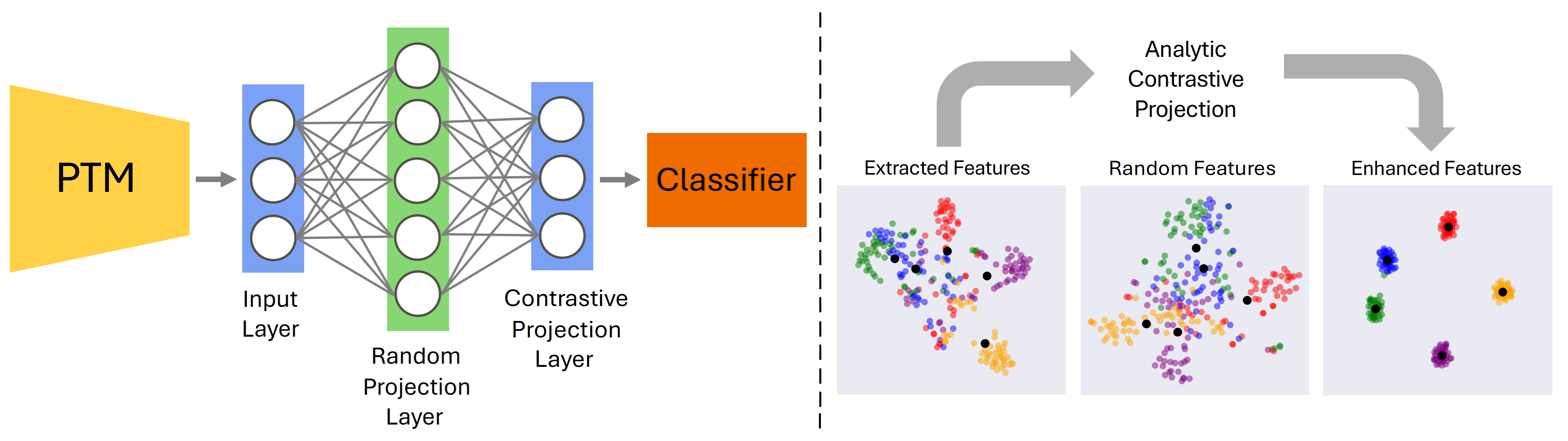
To overcome this limitation, we propose a novel analytic approach that also adapts feature representations for the continual learning tasks. The pipeline of our approach, illustrated in Figure 1 (left), begins with the PTM generating feature representations, termed the input layer. These features are transformed via a random projection (RP) layer into a higher-dimensional space Huang et al. (2011) and then passed through the contrastive projection (CP) layer, which enhances the class separability. The CP layer draws inspiration from contrastive learning, where the samples from the same class (positives) are drawn closer, while samples from different classes (negatives) are pushed apart, typically using a contrastive loss. However, applying this directly to CIL would lead to CF due to iterative gradient updates. We achieve similar effects via an analytic CP layer that can be incrementally updated as new tasks arrive. The impact of this CP layer on feature distribution is depicted in Figure 1 (right). Finally, a classifier layer makes the final predictions based on these adapted features.
4.1 Positive Alignment via Prototype Regression
We begin with the ELM formulation, where ridge regression is employed to map the features from the RP layer to the target vectors, as previously defined:
| (7) |
where represents the random feature obtained from the RP layer, and contains target vectors for inputs. When is one-hot encoded for classification, the cross matrix reduces to a matrix where each column is the sum of random features belonging to a given class. This can be factorized as:
| (8) |
Here, contains the class prototypes , defined as the means of the random features of class , and holds the number of samples per class. Both and can be computed incrementally as each task arrives.
This formulation can be extended to arbitrary targets. Instead of using one-hot vectors, we can assign each class a target prototype, representing its ideal position in the projected space. These target prototypes can have any dimensionality; however, to preserve the geometric structure of the representations, we set their dimension to match that of the input layer, . Let denote the target prototype matrix, where each row specifies the desired projection for class . For instance, can be set as the original class mean of the input layer, pulling the feature representations of class toward their respective mean. In this case, the cross matrix becomes:
| (9) |
This decomposition enables efficient incremental updates by maintaining class prototypes computed based on the features from the random projection layer, sample counts , and target prototypes . The learned projection maps samples toward their corresponding target prototypes, effectively pulling intra-class samples together and enhancing positive alignment.
4.2 Negative Repulsion via Target-Prototype Separation
Aligning input samples to their respective class means (using class means as target prototypes) improves intra-class compactness but does not guarantee adequate inter-class separation. In particular, some class means may lie close to each other in the feature space, making them hard to distinguish. To address this, we refine the target prototypes by shifting the class means to enhance the separation between classes.
Let denote the matrix of class means at the input layer. We normalize these means by whitening them with respect to the feature covariance matrix (shared by all classes). This adjustment is essential because a large variance in some dimensions can give a false impression of class separability. For example, in a low-variance dimension even a small separation is meaningful, whereas in high-variance dimensions, a much larger separation is needed to achieve the same effect. Whitening corrects for this imbalance by accounting for the variance of each feature dimension. The covariance is computed incrementally as Goswami et al. (2023):
| (10) |
where is the total number of samples seen up to task and is the set of classes introduced at task . We can then transform the class means as:
| (11) |
yielding whitened means with unit variance in all directions. We then perform singular value decomposition (SVD) on the whitened class means:
| (12) |
where is an orthonormal basis of the input space, defines the class means subspace, and is a diagonal matrix containing the singular values.
Our objective is to enhance the separation between class means, quantified by the sum of their pairwise cosine similarities. In principle, maximum separation would be achieved if the means were arranged uniformly on the surface of a hypersphere. However, this strict configuration would significantly alter the original data geometry, distorting the feature representations. To maintain the structure while increasing class separation, we introduce an adjustment to the singular values in , which perturbs the class means in directions that reduce their pairwise cosine similarities:
| (13) |
where is a scaling factor, and is defined in the following Lemma.
Lemma 4.1.
Denote as arbitrary vectors, and as a set of orthogonal bases of . Denote as the inner product and as the cosine similarity. There exist and
s.t.
| (14) |
See the proof in Appendix A. In Eq. 12, we denote and . Each in the subspace is perturbed by , effectively shifting it in an orthogonal direction with magnitude . By Lemma 4.1, there exist coefficients and a scalar such that Eq. 14 holds. The sign of each determines whether the shift occurs in the direction of or its opposite. This condition arises from the proof of Lemma 4.1, where we analyze the derivative of the function , defined as the sum of cosine similarities involving class . By selecting accordingly, we ensure that the slope of at is negative, which guarantees that a small positive decreases the cosine similarity. The choice of is also important: if is too small, the shift becomes negligible, whereas if it is too large, the reduction in cosine similarity may no longer be valid. In practice, we set in our experiments.
Defining , the lemma guarantees that the average cosine similarity among the columns of is smaller than that of . Since the columns of form an orthogonal basis in , the transformations preserve inner products and norms:
| (15) |
Thus, the cosine similarity between transformed vectors remains the same, i.e., . Therefore, the average cosine similarity among the columns of is also reduced compared to the original matrix .
Note that separability is measured as the sum of cosine similarities, but the class means are whitened. This procedure is closely related to Mahalanobis distance, which has been shown to outperform cosine similarity in related contexts Goswami et al. (2023). By whitening, we effectively assess separation using Mahalanobis distance; after increasing the separation, we de-whiten the features to restore their original scale:
| (16) |
The separated class means are then used as target prototypes for the CP layer by setting in Eq. 9 to , aligning samples with their respective classes while enhancing the separation between classes.
4.3 Classifier
The CP layer is an analytic module that adapts feature representations across tasks without modifying the underlying PTM. To increase its capacity, we extend it with multiple random projections. Since each RP is initialized independently, we learn a corresponding CP for each RP, all sharing the same set of target prototypes. Specifically, we define such heads, where each CP head maps the random features to the same target prototype space. Given an input , each head produces a projection and the output is obtained by averaging across heads:
| (17) |
This aggregated representation is then classified using NCM, which assigns it to the nearest target prototype in . As shown in Table 3 (row 3), AnaCP with an NCM classifier already outperforms all baselines. However, NCM is often surpassed by more expressive classifiers. To further improve performance, we place an ELM classifier after the averaged CP representation.
Unlike PTM features and their random projections, which remain fixed, the CP outputs evolve as new tasks are introduced due to the incremental computation of the CP layer. Directly updating the ELM classifier incrementally (Eq. 3) may therefore lead to CF. To mitigate this, we employ a pseudo-replay strategy. We model the PTM features (input layer) as a multivariate Gaussian distribution parameterized by the class means and a shared covariance matrix, from which we generate pseudo-replay samples for training. This approach resembles that of Zhang et al. (2023), which also trains the classifier on generated features. However, whereas Zhang et al. (2023) maintains a separate covariance matrix per class (leading to memory cost that grows with the number of classes), we use a single shared covariance matrix across all classes. This design significantly reduces memory usage while yielding comparable performance. Specifically, we reuse the class means and shared covariance matrix from Eq. 10 for feature generation. The generated samples are then processed by the RP and CP layers to form the classifier input, upon which the ELM is trained using Eq. 6.
5 Experiments
5.1 Experimental Setup
Datasets: We conduct experiments on five publicly available datasets: CIFAR100 (100 classes) (Krizhevsky et al., 2009), ImageNet-R (200 classes) (Hendrycks et al., 2021), CUB (200 classes) (Wah et al., 2011), TinyImageNet (200 classes) (Le and Yang, 2015), and Cars (196 classes) (Yang et al., 2015). For all datasets, we use the official train and test splits. Each dataset is split into 10 disjoint tasks by shuffling classes, and experiments are repeated with three different random seeds to account for variability in class-task assignments.
Baselines: We compare AnaCP with a range of baselines, including prompt-learning methods (L2P (Wang et al., 2022c), DualPrompt (Wang et al., 2022b), and CODA-Prompt (Smith et al., 2023)), fine-tuning method (SLCA Zhang et al. (2023)), and analytic methods that treat the PTM as a frozen feature extractor. The analytic baselines include SimpleCIL (Janson et al., 2022), SLDA (Hayes and Kanan, 2020), KLDA (Momeni et al., 2025), GACL (Zhuang et al., 2024), APER (Zhou et al., 2024), FeCAM (Goswami et al., 2023), and RanPac McDonnell et al. (2023), with some incorporating FSA. For a complete performance perspective, we also include results from joint linear probe, where a linear softmax classifier is trained on the PTM features using gradient descent with all tasks’ data, and joint fine-tuning, which directly fine-tunes the PTM on the entire dataset and serves as the upper bound for CIL performance.
Implementation Details: For the PTMs, we use DINO-v2 (Oquab et al., 2023) and MoCo-v3 (Chen et al., 2021), both of which are self-supervised PTMs. This choice helps prevent information leakage, as supervised PTMs are exposed to class labels during training, some of which may reappear in CIL, leading to unintended information leakage. MoCo-v3 is pre-trained on ImageNet-1k – a commonly used but relatively small dataset for pre-training in prior studies. However, because ImageNet-1k (or even ImageNet-21k) is considered limited for real-world applications, we also utilize DINO-v2, a more powerful model pre-trained on the substantially larger LVD-142M dataset. For joint fine-tuning, we employ LoRA adapters (Hu et al., 2021) instead of full fine-tuning, as we found this approach to be more accurate.
The prompt learning baselines are taken from the (Smith et al., 2023) repository, while SLCA, FeCAM, and RanPac are evaluated using their original implementations. All remaining analytic baselines are incorporated into a unified experimental setup, following their official implementations to ensure fair comparison.111The code of AnaCP is available at https://github.com/SalehMomeni/AnaCP. We also adopt FSA following (Zhou et al., 2024) before applying AnaCP to the frozen PTM as it helps improve accuracy. We use RP dimension , number of CP heads , and number of generated feature representations per class for the classifier as the default configuration; ablations on other variants are included. The regularization parameter in Eq. 6 for ELM is set to , and the coefficient for class mean repulsion is set to 1. These values were optimized on a validation set derived from the CIFAR100 training set and are consistently used across all datasets and both PTMs. All experiments are conducted on a single NVIDIA A100 GPU with 80GB VRAM.
Evaluation Metric: We evaluate model performance using two primary metrics: Last Accuracy (), the accuracy after completing all tasks, and Average Incremental Accuracy (), calculated as , where denotes the accuracy at the end of task . Additionally, we measure running time and memory efficiency to assess the practicality of the methods. We also define relative error reduction as , where is the baseline accuracy and is the improved accuracy.
Method CIFAR100 ImageNet-R CUB TinyImageNet Cars Joint linear probe - - - - - Joint fine-tuning - - - - - L2P DualPrompt CODA-Prompt SLCA SimpleCIL SLDA KLDA GACL APER FeCAM RanPAC AnaCP - AnaCP Rel. Error
Method CIFAR100 ImageNet-R CUB TinyImageNet Cars Joint linear probe - - - - - Joint fine-tuning - - - - - SLCA SimpleCIL SLDA KLDA GACL APER FeCAM RanPAC AnaCP - AnaCP Rel. Error
5.2 Comparison with Baselines
Table 1 presents the main results of our experiments, with all methods using DINO-v2 as the PTM. AnaCP consistently outperforms all baselines across the evaluated datasets, achieving an absolute improvement in last accuracy ranging from 1.03% to 3.17% across different datasets, corresponding to a relative error reduction between 4.8% and 31.4%. We can observe that using replay features with a shared covariance (AnaCP) achieves similar results to class-specific covariances (AnaCP - ) while significantly reducing the number of parameters. AnaCP also surpasses the joint linear probe on all datasets and achieves comparable accuracy to joint fine-tuning, which represents the upper bound for CIL. Notably, on two datasets, AnaCP even exceeds this upper bound, while on the remaining datasets, the largest accuracy gap is only around 2%. These results highlight that AnaCP’s feature adaptation is highly effective, even without directly training the PTM on each task.
We also evaluate AnaCP using MoCo-v3 as the PTM, as presented in Table 2. AnaCP outperforms the baselines by a larger margin with MoCo-v3 than with DINO-v2, as the weaker features of MoCo-v3 make the CP layer more impactful. In this case, the gap to joint fine-tuning increases to 6%, which is expected since MoCo-v3 is a weaker PTM and benefits more from full fine-tuning. However, given that both PTMs have the same architecture (number of layers and hidden size), there is no reason to prefer a weaker PTM in real-world applications.
5.3 Analysis of Catastrophic Forgetting
The CP layer in our method is inherently immune to CF, as it operates on a frozen PTM and updates its statistics (prototypes and the Gram matrix) incrementally without overwriting prior information. In contrast, the final ELM classifier relies on pseudo-replay, which in principle could introduce some forgetting. In practice, however, we found this effect to be minimal. To verify this, we evaluate under the task-incremental learning (TIL) setting, where the task identity is provided at inference time. Specifically, we present the accuracy matrix , where each entry denotes the accuracy on task after training on the first tasks of CIFAR-100 (10-task split) using DINO-v2 as the backbone.

We adopt the TIL setting for this analysis because it offers a clearer view of forgetting. In CIL, accuracy inevitably decreases as more tasks are introduced, not necessarily due to forgetting, but because the classification problem becomes harder with a growing number of classes. By contrast, TIL keeps the classification difficulty fixed, since each task has a constant number of classes and the task ID is known at inference. Under this setup, forgetting would appear as a decline in accuracy on earlier tasks. However, as shown in Figure 2, the accuracy for task 1 (first column) remains nearly constant across all steps. The same holds for other tasks, demonstrating that our method effectively preserves knowledge from prior tasks.
row CLS CP NR H D R CIFAR100 ImageNet-R CUB TinyImageNet Cars 1 NCM ✗ - - - - 88.13±0.21 81.60±0.08 86.95±0.36 83.63±0.48 69.51±0.87 2 NCM ✓ ✗ 3 5000 - 91.31±0.03 83.29±0.45 89.52±0.10 85.89±0.26 86.25±0.25 3 NCM ✓ ✓ 3 5000 - 91.86±0.05 86.01±0.11 89.88±0.32 87.02±0.27 89.48±0.29 4 ELM ✗ - - 5000 - 91.12±0.10 85.14±0.26 89.75±0.19 86.48±0.12 89.32±0.20 5 ELM ✓ ✗ 3 5000 100 91.87±0.02 85.73±0.19 90.39±0.14 86.69±0.28 90.24±0.20 6 ELM ✓ ✓ 3 5000 100 92.15±0.09 86.60±0.04 90.48±0.15 87.71±0.29 90.65±0.24 7 ELM ✓ ✓ 3 5000 20 92.14±0.06 86.39±0.04 90.43±0.18 87.29±0.32 90.45±0.23 8 ELM ✓ ✓ 3 5000 50 92.13±0.04 86.47±0.05 90.46±0.10 87.49±0.32 90.57±0.16 9 ELM ✓ ✓ 3 5000 100 92.15±0.09 86.60±0.04 90.48±0.15 87.71±0.29 90.65±0.24 10 ELM ✓ ✓ 1 5000 100 91.99±0.01 85.72±0.24 90.36±0.13 87.12±0.24 90.35±0.24 11 ELM ✓ ✓ 3 5000 100 92.15±0.09 86.60±0.04 90.48±0.15 87.71±0.29 90.65±0.24 12 ELM ✓ ✓ 5 5000 100 92.20±0.04 86.62±0.10 90.51±0.05 87.76±0.29 90.68±0.18 13 ELM ✓ ✓ 3 1000 100 90.64±0.10 84.01±0.29 89.56±0.15 85.48±0.17 88.23±0.21 14 ELM ✓ ✓ 3 2000 100 91.35±0.08 85.15±0.19 89.97±0.18 86.24±0.22 89.93±0.10 15 ELM ✓ ✓ 3 5000 100 92.15±0.09 86.60±0.04 90.48±0.15 87.71±0.29 90.65±0.24 16 ELM ✓ ✓ 3 10000 100 92.75±0.10 86.86±0.10 90.60±0.10 88.11±0.24 90.73±0.16
5.4 Ablation Studies
We conduct a series of ablations to evaluate the impact of key components, as shown in Table 3. Rows 1-3 examine the effect of the CP layer. Removing CP and directly applying an NCM classifier to PTM features results in a significant drop in absolute accuracy between 2.93% to 19.97% (row 1 vs. row 3). This highlights the importance of CP in enhancing feature representations, as illustrated in Figure 1. The effect of negative repulsion (NR), which increases the separation between class means (Section 4.2) is also evident; disabling NR and relying only on positive alignment with the original class means as target prototypes leads to an accuracy reduction from 0.38% to 3.23% (row 2 vs. row 3). This confirms that NR is a critical component for improving class separability.
The role of classifier is explored in Rows 4-6, where NCM is replaced by ELM. We find that using an ELM classifier on average improves the performance by 0.66% (row 3 vs. row 6). Although this requires generating feature representations as pseudo-replay for training the ELM classifier, as explained in Section 4.3. An arbitrary number of feature representations can be sampled from the Gaussian distribution with negligible computational overhead, as detailed in the running time analysis. We observe that increasing the number of generated feature representations improves performance on some datasets (Rows 7-9). The effects of various numbers of CP heads (Rows 10-12) and RP dimensions (Rows 13-16) are also explored. Generally, increasing these values improves accuracy, albeit at the cost of additional parameters. For the main results, we have used and . We note that even with , AnaCP outperforms all baselines.
5.5 Memory and Running Time Efficiency
AnaCP needs to save class means, each of size , and a shared covariance matrix of size for feature whitening and pseudo-replay feature generation at the input layer (Figure 1). While a separate covariance matrix can be maintained for each class, this would result in a significant increase in memory as the number of classes grows. As shown in Table 1, using a shared covariance matrix does not compromise accuracy. Each CP head maintains the following: (1) an RP matrix of size , (2) a Gram matrix, (3) class prototypes (or means) in the random feature space, each of size , and (4) a projection matrix of size . We have such heads in total. The target prototypes do not need to be stored, as they can be derived from the class means. The classifier layer also maintains an RP matrix of size and of size . Unlike the CP layer, this layer doesn’t need to store the Gram matrix for incremental updates, as it is computed from generated feature representations after each task.
For a typical configuration with , , , and , the total number of stored parameters amounts to approximately 106.6 million. The majority of these parameters belong to the Gram matrices, which does not increase with the number of classes. Also, none of these parameters are trainable, making them suitable for storage in reduced-precision formats such as float8. This would further reduce the total memory usage to approximately 102 MiB.
While AnaCP may have a higher parameter count compared to some other methods, the design is balanced with exceptional computational efficiency. For example, CIFAR100 with the DINO-v2 PTM requires only 9 minutes and 18 seconds for training. 6 minutes and 5 seconds of this time are dedicated to the FSA, and 3 minutes and 8 seconds are spent passing inputs through the PTM to extract features. The core operations of AnaCP, including updating the CP layer and training the classifier with generated features, collectively take only 5 seconds. Thus, despite the larger parameter count, these operations are extremely fast. For comparison, a baseline such as CODA-Prompt that requires task-specific training takes 3 hours and 47 minutes to complete training on CIFAR100, and joint fine-tuning requires 1 hour and 58 minutes.
5.6 Discussion
Our results support the proposition that a strong PTM is the key to CL, and that representation-level forgetting is not the primary limitation. Even simple CIL strategies, when paired with a fixed PTM, can achieve near-optimal performance. This view aligns with neuroscience evidence that the human brain maintains stable representations, despite minor drift over time (Gonzalez et al., 2019; Roth and Merriam, 2023). Cortical activity also preserves a stable similarity structure that supports consistent perception and behavior, even as neural responses gradually shift (McMahon et al., 2014; Roth and Merriam, 2023). The human brain can thus be viewed as an innate PTM refined through evolution, which provides a stable foundation for continual adaptation. Similarly, large-scale pre-training in machine learning resembles this biological evolution and development, producing reusable representations that enable CL without any forgetting. For further discussion, see Momeni and Liu (2025).
6 Conclusion
CIL poses a significant challenge in continual learning. Recent analytic methods with PTMs have shown promise. However, since they cannot learn or adapt features obtained from PTMs to suit specific CIL tasks, their performance is still suboptimal. This paper proposed a novel and principled method, called AnaCP, to adapt features extracted from PTMs analytically, which offers a highly efficient and accurate solution for CIL. Empirical evaluations demonstrate that AnaCP outperforms strong baselines, but more importantly, if paired with a strong PTM, its accuracy can be comparable to the joint training upper bound.
Limitations: When using a strong PTM like DINO-v2, AnaCP achieves accuracy on par with the joint fine-tuning upper bound. However, with a weaker PTM such as MoCo-v3, AnaCP cannot match joint fine-tuning accuracy due to the critical role of PTM features played in our method. While strong PTMs are readily available today, improving AnaCP’s performance with weaker PTMs remains a meaningful goal. Additionally, our work currently focuses CIL. We believe AnaCP can be extended to TIL and domain-incremental learning (DIL) scenarios with appropriate adaptations.
Acknowledgments
The work of Saleh Momeni and Bing Liu was supported in part by three NSF grants (IIS-2229876, IIS-1910424, and CNS-2225427), and an NVIDIA’s Academia Grant, which provides cloud compute via its Saturn Cloud.
References
- [1] (2019) Online continual learning with maximal interfered retrieval. Advances in neural information processing systems 32. Cited by: §2.
- [2] (2020) Dark experience for general continual learning: a strong, simple baseline. Advances in neural information processing systems 33, pp. 15920–15930. Cited by: §2.
- [3] (2020) Continual learning in low-rank orthogonal subspaces. Advances in Neural Information Processing Systems 33, pp. 9900–9911. Cited by: §2.
- [4] (2020) A simple framework for contrastive learning of visual representations. In International conference on machine learning, pp. 1597–1607. Cited by: §1.
- [5] (2021) An empirical study of training self-supervised vision transformers. In 2021 IEEE/CVF International Conference on Computer Vision (ICCV), pp. 9620–9629. Cited by: §5.1.
- [6] (2018) Lifelong machine learning. Synthesis Lectures on Artificial Intelligence and Machine Learning 12 (3), pp. 1–207. Cited by: §1.
- [7] (2021) Continual learning for task-oriented dialogue system with iterative network pruning, expanding and masking. In Proceedings of the 59th Annual Meeting of the Association for Computational Linguistics (ACL/IJCNLP), Cited by: §2.
- [8] (2022) Continual pre-training of language models for math problem understanding with syntax-aware memory network. In Proceedings of the 60th Annual Meeting of the Association for Computational Linguistics (Volume 1: Long Papers), pp. 5923–5933. Cited by: §2.
- [9] (2019) Persistence of neuronal representations through time and damage in the hippocampus. Science 365 (6455), pp. 821–825. Cited by: §5.6.
- [10] (2023) Fecam: exploiting the heterogeneity of class distributions in exemplar-free continual learning. Advances in Neural Information Processing Systems 36, pp. 6582–6595. Cited by: §1, §2, §4.2, §4.2, §5.1.
- [11] (2022) DEMix layers: disentangling domains for modular language modeling. In Proceedings of the 2022 Conference of the North American Chapter of the Association for Computational Linguistics, pp. 5557–5576. Cited by: §2.
- [12] (2020) Lifelong machine learning with deep streaming linear discriminant analysis. In Proceedings of the IEEE/CVF conference on computer vision and pattern recognition workshops, pp. 220–221. Cited by: §2, §5.1.
- [13] (2021) The many faces of robustness: a critical analysis of out-of-distribution generalization. In Proceedings of ICCV, pp. 8340–8349. Cited by: §5.1.
- [14] (2015) Distilling the knowledge in a neural network. arXiv preprint arXiv:1503.02531. Cited by: §2.
- [15] (2021) LoRA: low-rank adaptation of large language models. In International Conference on Learning Representations, Cited by: §5.1.
- [16] (2011) Extreme learning machine for regression and multiclass classification. IEEE Transactions on Systems, Man, and Cybernetics, Part B (Cybernetics) 42 (2), pp. 513–529. Cited by: §1, §2, §3, §4.
- [17] (2022) A simple baseline that questions the use of pretrained-models in continual learning. arXiv preprint arXiv:2210.04428. Cited by: §2, §5.1.
- [18] (2023) Generating instance-level prompts for rehearsal-free continual learning. In Proceedings of the IEEE/CVF International Conference on Computer Vision, pp. 11847–11857. Cited by: §2.
- [19] (2021) Achieving forgetting prevention and knowledge transfer in continual learning. Advances in Neural Information Processing Systems 34. Cited by: §1, §2.
- [20] (2022) Continual learning of natural language processing tasks: a survey. arXiv preprint arXiv:2211.12701. Cited by: §1.
- [21] (2020) Supervised contrastive learning. Advances in neural information processing systems 33, pp. 18661–18673. Cited by: §1.
- [22] (2022) A theoretical study on solving continual learning. Advances in neural information processing systems 35, pp. 5065–5079. Cited by: §2.
- [23] (2023) Learnability and algorithm for continual learning. In International Conference on Machine Learning, pp. 16877–16896. Cited by: §1.
- [24] (2017) Overcoming catastrophic forgetting in neural networks. Proceedings of the national academy of sciences 114 (13), pp. 3521–3526. Cited by: §2.
- [25] (2009) Learning multiple layers of features from tiny images. Cited by: §5.1.
- [26] (2015) Tiny imagenet visual recognition challenge. CS 231N 7, pp. 7. Cited by: §5.1.
- [27] (2022) Overcoming catastrophic forgetting during domain adaptation of seq2seq language generation. In Proceedings of the 2022 Conference of the North American Chapter of the Association for Computational Linguistics: Human Language Technologies, Cited by: §2.
- [28] (2006) A fast and accurate online sequential learning algorithm for feedforward networks. IEEE Transactions on neural networks 17 (6), pp. 1411–1423. Cited by: §1, §3.
- [29] (2024) Inflora: interference-free low-rank adaptation for continual learning. In Proceedings of the IEEE/CVF Conference on Computer Vision and Pattern Recognition, pp. 23638–23647. Cited by: §2.
- [30] (2024) Class incremental learning via likelihood ratio based task prediction. ICLR-2024. Cited by: §1, §2, §2.
- [31] (2023) Continual learning for multilingual neural machine translation via dual importance-based model division. In Proceedings of the 2023 Conference on Empirical Methods in Natural Language Processing, pp. 12011–12027. Cited by: §2.
- [32] (2021) Lifelong intent detection via multi-strategy rebalancing. arXiv preprint arXiv:2108.04445. Cited by: §2.
- [33] (2019) Continual learning for sentence representations using conceptors. In Proceedings of the 2019 Conference of the North American Chapter of the Association for Computational Linguistics: Human Language Technologies, NAACL-HLT 2019, Minneapolis, MN, USA, June 2-7, 2019, Volume 1 (Long and Short Papers), Cited by: §2.
- [34] (2020) Generative feature replay for class-incremental learning. In Proceedings of the IEEE/CVF conference on computer vision and pattern recognition workshops, pp. 226–227. Cited by: §2.
- [35] (1989) Catastrophic interference in connectionist networks: The sequential learning problem. In Psychology of learning and motivation, Vol. 24, pp. 109–165. Cited by: §1.
- [36] (2023) Ranpac: random projections and pre-trained models for continual learning. Advances in Neural Information Processing Systems (NeurIP-2023) 36. Cited by: §1, §1, §2, §2, §5.1.
- [37] (2014) Face-selective neurons maintain consistent visual responses across months. Proceedings of the National Academy of Sciences 111 (22), pp. 8251–8256. Cited by: §5.6.
- [38] (2025) Achieving upper bound accuracy of joint training in continual learning. arXiv preprint arXiv:2502.12388. Cited by: §5.6.
- [39] (2025) Continual learning using a kernel-based method over foundation models. In AAAI-2025, Cited by: §1, §1, §2, §2, §5.1.
- [40] (2023) DINOv2: learning robust visual features without supervision. Transactions on Machine Learning Research. Cited by: §5.1.
- [41] (2005) Incremental linear discriminant analysis for classification of data streams. IEEE transactions on Systems, Man, and Cybernetics, part B (Cybernetics) 35 (5), pp. 905–914. Cited by: §2.
- [42] (2023) First session adaptation: a strong replay-free baseline for class-incremental learning. In Proceedings of the IEEE/CVF International Conference on Computer Vision, pp. 18820–18830. Cited by: §1.
- [43] (2025) LoRanPAC: low-rank random features and pre-trained models for bridging theory and practice in continual learning. ICLR. Cited by: §2.
- [44] (2023) Lifelong sequence generation with dynamic module expansion and adaptation. In Proceedings of the 2023 Conference on Empirical Methods in Natural Language Processing, pp. 6701–6714. Cited by: §2.
- [45] (2022) ELLE: efficient lifelong pre-training for emerging data. In Findings of the Association for Computational Linguistics: ACL 2022, pp. 2789–2810. Cited by: §2.
- [46] (2020) Itaml: an incremental task-agnostic meta-learning approach. In Proceedings of the IEEE/CVF Conference on Computer Vision and Pattern Recognition, pp. 13588–13597. Cited by: §2.
- [47] (2023) Representations in human primary visual cortex drift over time. Nature Communications 14 (4422). Cited by: §5.6.
- [48] (2024) Convolutional prompting meets language models for continual learning. In Proceedings of the IEEE/CVF Conference on Computer Vision and Pattern Recognition, pp. 23616–23626. Cited by: §2.
- [49] (2019) Theory of ridge regression estimation with applications. John Wiley & Sons. Cited by: §3.
- [50] (2018) Overcoming catastrophic forgetting with hard attention to the task. In International Conference on Machine Learning, pp. 4548–4557. Cited by: §2.
- [51] (2021) Online class-incremental continual learning with adversarial shapley value. In Proceedings of the AAAI Conference on Artificial Intelligence, Vol. 35, pp. 9630–9638. Cited by: §2.
- [52] (2023) Coda-prompt: continual decomposed attention-based prompting for rehearsal-free continual learning. In Proceedings of the IEEE/CVF conference on computer vision and pattern recognition, pp. 11909–11919. Cited by: §2, §5.1, §5.1.
- [53] (2025) Mos: model surgery for pre-trained model-based class-incremental learning. In Proceedings of the AAAI Conference on Artificial Intelligence, Vol. 39, pp. 20699–20707. Cited by: §2.
- [54] (2020) Brain-inspired replay for continual learning with artificial neural networks. Nature communications 11 (1), pp. 4069. Cited by: §2.
- [55] (2019) Three scenarios for continual learning. arXiv preprint arXiv:1904.07734. Cited by: §1.
- [56] (2011) The caltech-ucsd birds-200-2011 dataset. Cited by: §5.1.
- [57] (2022) BEEF: bi-compatible class-incremental learning via energy-based expansion and fusion. In The Eleventh International Conference on Learning Representations, Cited by: §2.
- [58] (2023) Hierarchical decomposition of prompt-based continual learning: rethinking obscured sub-optimality. Advances in Neural Information Processing Systems 36, pp. 69054–69076. Cited by: §2.
- [59] (2024) A comprehensive survey of continual learning: theory, method and application. IEEE Transactions on Pattern Analysis and Machine Intelligence. Cited by: §1.
- [60] (2024) Rehearsal-free modular and compositional continual learning for language models. In Proceedings of the 2024 Conference of the North American Chapter of the Association for Computational Linguistics: Human Language Technologies (Volume 2: Short Papers), pp. 469–480. Cited by: §2.
- [61] (2022) Dualprompt: complementary prompting for rehearsal-free continual learning. In European Conference on Computer Vision, pp. 631–648. Cited by: §2, §5.1.
- [62] (2022) Learning to prompt for continual learning. In Proceedings of the IEEE/CVF Conference on Computer Vision and Pattern Recognition, pp. 139–149. Cited by: §1, §2, §5.1.
- [63] (2020) Supermasks in superposition. Advances in Neural Information Processing Systems 33, pp. 15173–15184. Cited by: §2.
- [64] (2021) Der: dynamically expandable representation for class incremental learning. In Proceedings of the IEEE/CVF Conference on Computer Vision and Pattern Recognition, pp. 3014–3023. Cited by: §2.
- [65] (2015) A large-scale car dataset for fine-grained categorization and verification. In Proceedings of the IEEE conference on computer vision and pattern recognition, pp. 3973–3981. Cited by: §5.1.
- [66] (2024) Recent advances of foundation language models-based continual learning: a survey. ACM Computing Surveys. Cited by: §1.
- [67] (2017) Continual learning through synaptic intelligence. In International Conference on Machine Learning, pp. 3987–3995. Cited by: §2.
- [68] (2023) Slca: slow learner with classifier alignment for continual learning on a pre-trained model. In Proceedings of the IEEE/CVF International Conference on Computer Vision, pp. 19148–19158. Cited by: §1, §2, §4.3, §5.1.
- [69] (2024) Revisiting class-incremental learning with pre-trained models: generalizability and adaptivity are all you need. International Journal of Computer Vision. Cited by: §2, §5.1, §5.1.
- [70] (2022) Self-sustaining representation expansion for non-exemplar class-incremental learning. In Proceedings of the IEEE/CVF conference on computer vision and pattern recognition, pp. 9296–9305. Cited by: §2.
- [71] (2024) GACL: exemplar-free generalized analytic continual learning. In Advances in Neural Information Processing Systems, Cited by: §2, §2, §5.1.
- [72] (2022) ACIL: analytic class-incremental learning with absolute memorization and privacy protection. Advances in Neural Information Processing Systems 35, pp. 11602–11614. Cited by: §1, §2, §2, §3.
Appendix A Technical Appendices
Lemma A.1 (Lemma 4.1).
Denote as arbitrary vectors, and as a set of orthogonal bases of . Denote as the inner product and as the cosine similarity. There exist and
s.t.
| (18) |
Proof.
Let
For simplicity, denote
and
Therefore, we have
Since , we have
Since , we have
Therefore, we have
which shows that ’s defined above guarantee .
Let
Since is a continuous function, we could take a sufficiently small s.t. has the same sign when . Then for , the ’s defined above also guarantee . Choosing gives the result. ∎