Just Few States are Enough: Randomized Sparse Feedback for Stability of Dynamical Systems
Abstract
While classical control theory assumes that the controller has access to measurements of the entire state (or output) at every time instant, this paper investigates a setting where the feedback controller can only access a randomly selected subset of the state vector at each time step. Due to the random sparsification that selects only a subset of the state components at each step, we analyze the stability of the closed-loop system in terms of Asymptotic Mean-Square Stability (AMSS), which ensures that the system state converges to zero in the mean-square sense. We consider the problem of designing both a feedback gain matrix and a measurement sparsification strategy that minimizes the number of state components required for feedback, while ensuring AMSS of the closed-loop system. Interestingly, (1) we provide conditions on the dynamics of the system under which it is possible to find a sparsification strategy, and (2) we propose a Linear Matrix Inequality (LMI) based algorithm that jointly computes a stabilizing gain matrix, and a randomized sparsification strategy that minimizes the expected number of measured state coordinates while preserving the AMSS. Our approach is then extended to the case where the sparsification probabilities vary across the state components. Based on these theoretical findings, we propose an algorithmic procedure to compute the vector of sparsification parameters, along with the corresponding feedback gain matrix. To the best of our knowledge, this is the first study to investigate the stability properties of control systems that rely solely on randomly selected state measurements. Numerical simulations demonstrate that, in some settings, the system achieves comparable performance to full-state feedback while requiring measurements from only of the state coordinates.
Introduction
In control theory, the primary objective is to design control strategies that ensure a system behaves according to a desired specification (Åström and Murray 2021). Among the most fundamental specifications is the requirement for the system to converge to a specific operating point, most commonly the origin (Khalil 2009). This property, known as stabilization to the origin, is essential in many applications where the system must settle into a rest state or nominal condition after initial transients (Hespanha 2018). Achieving this goal typically involves the design of a feedback controller that adjusts the input based on the system’s current state, ensuring asymptotic convergence to the origin.
In closed-loop control systems, feedback is critical for ensuring asymptotic stability, but measuring the full state vector can be resource-intensive, particularly in high-dimensional systems or constrained environments. To address this, we introduce in this paper a novel control paradigm in which the controller accesses only a randomly selected subset of the state vector at each time step. A clear motivation for incorporating sparsity in control design stems from recent technological advances that have enabled individual components of large-scale systems to integrate their sensing, actuation, communication, computation, and decision-making capabilities.
In this paper, we study the AMSS of linear discrete-time systems under a feedback control strategy with access to a randomized sparse state vector. Our main objective is to minimize the expected sparsity, the average number of active sensors, while ensuring AMSS. To this end, we introduce randomized sparsification strategies and analyze the system’s expected dynamics. We show that the expected state converges to zero if the closed-loop system is deterministically asymptotically stable. We then formally define expected sparsity and study the system’s variance, with a focus on stabilizing the system using the minimum expected number of sensors. We derive conditions under which AMSS can be achieved and propose algorithms that jointly design the feedback controller along with the sparsification probabilities minimizing the expected sparsity. Finally, we validate our results through experiments. Proofs are provided in Appendix A, and additional experiments in Appendix B.
Our contributions are summarized as follows:
-
•
First study of randomized sparse-feedback control: Providing sufficient conditions for the system dynamics to support randomized sparsification and integrating these conditions into controller design that ensures minimum expected sparsity while achieving AMSS of the system.
-
•
Extension to adaptive sparsification: Tailored sparsification strategies for each state vector component to enable flexible adjustment of sparsity based on the difficulty of operating or measuring the state component.
-
•
Efficiency and practicality: Experimental results underscore the practical impact of this work, demonstrating that the proposed approach achieves performance comparable to full-state feedback while requiring measurements from only of state coordinates in some settings. This drastic reduction in measurement requirements is a game-changer for large-scale systems, where sensing all state variables is often infeasible due to cost, energy, or bandwidth limitations.
Related work
Asymptotic stability via deterministically-sparse feedback controllers.
Numerous works deal with the sparsity of the control gain matrix to reduce sensor/actuator usage and communication bandwidth, which applies to networked control systems or large-scale systems. For instance, in (Bykov and Shcherbakov 2018), the authors focused on sparsity in the control gain matrix (zero rows in ) to reduce the number of control inputs. Another way to achieve sparsity deterministically is by minimizing the norm, which leads to a gain matrix with zero columns or rows (Lin et al. 2012), (Polyak et al. 2014). The sparsity structure is fixed and designed a priori, see (Polyak et al. 2013) for details. Furthermore, in (Sun et al. 2025), the authors introduced a mixed-integer programming approach to address row cardinality constraints, in contrast to the norm-based convexification method. However, all these approaches mainly focus on deterministic sparsity. Moreover, in (Sriram et al. 2023), the authors provide sufficient and necessary conditions for achieving stability using -sparse control inputs. Their work only deals with deterministic sparsity under open-loop control strategies where the control inputs depend only on the initial point and parameters of the system. As stated in (Bishop 2011), open-loop control strategies, lacking feedback, can not adapt to disturbances or parameter variations, resulting in unreliable performance. Our work presents an analysis of randomized sparsity and deals with the stability of closed-loop systems.
Sparsity in distributed learning. In the context of limited access to the full state, (Cheng et al. 2021) addresses efficient data representation to maintain control performance by focusing on compressing high-dimensional time series data, such as cellular demand or electricity load, into a low-dimensional representation to reduce communication over a bandwidth-constrained network. Our work is also inspired by gradient vector sparsification used in the context of distributed machine learning. For example, in (Wangni et al. 2018), the authors introduce a sparsification technique that minimizes communication costs while keeping the increase in gradient variance small, ensuring that the optimization algorithm converges with only a slight increase in iterations.
Sensor scheduling. The existing literature on sensor scheduling can be grouped into three main directions: (1) Several approaches (Maity et al. 2022; Vitus et al. 2012) analyze randomness in settings where sensors communicate over constrained channels to remote estimators, focusing on estimation performance only and not on controller synthesis. (2) Other works, such as (Kundu and Quevedo 2019), examine scenarios with multiple systems sharing a communication channel, where periodic scheduling is combined with randomness arising from network-induced losses. (3) Continuous-time co-design approaches such as (Nugroho et al. 2019) provide time-invariant deterministic schedules.
To the best of our knowledge, the proposed approach in our paper is the first framework that jointly designs time-varying randomized sensor selection procedures together with the control gain to ensure global mean-square asymptotic stability.
Preliminaries
Mathematical Notations
We denote by the two norm on . The -by- identity matrix is denoted by . Given , we denote by the set of all eigenvalues of , by the spectral radius of , by the spectral norm of given by: , by the transpose of , by the column vector of , and by a diagonal matrix whose diagonal entries are the diagonal elements of . For simplification, we denote also by a diagonal matrix of order with diagonal coefficients . Given , we denote by the set of stabilizing control gain matrices defined by . We denote by a Bernoulli random variable of parameter where represents the probability of success. The notation is equivalent to the matrix being positive definite.
Randomized Sparsification Strategies
Consider a discrete-time control systems of the form:
| (1) |
where is a state, is a control input, and are matrices with appropriate dimensions. In the sequel, we assume that the system is stabilizable, i.e, there exists a feedback gain matrix such that , (Grüne 2000). In this paper, we consider the case where, at each time step , the controller has only access to a randomly selected portion of the full state , i.e the control inputs are of the form . More specifically, at each time step k, contains a random subset of the coordinates of , and the remaining coordinates are set to zero. The portion of the state accessed is selected randomly according to a time-varying map , which is a diagonal matrix of the form , where are independent random variables, each determines whether the corresponding coordinate in is included in or set to zero at time . More precisely, we randomly drop out the -th coordinate with a probability of , which means the coordinate remains non-zero with a probability of . To preserve the unbiasedness of the sparsified state vector , each non-zero coordinate is scaled by , resulting in . Thus, our sparsification matrix at each time step becomes: , and are random Bernoulli variables of parameter respectively. In the rest of the paper, we will analyze the stability properties of the closed-loop system consisting of the discrete-time control system in Eq.1 under the feedback controller , for a gain and the sparsification matrix defined above. The dynamics of the closed-loop system is given by:
| (2) |
This random sparsification aims to reduce financial costs (equipment, maintenance) and computational costs (processing time, energy) incurred from measuring the system’s state vector (e.g., position, velocity) for computing control inputs, which depend on sensors, data acquisition, and processing (Zhong et al. 2024). As such, in this paper, we study two sparsification scenarios:
-
1.
The case where are where , and
(3) -
2.
The adaptive sparsification case where are , and the sparsification matrix is given by:
(4)
This second scenario allows for more flexibly. It supports the prioritization of sensor monitoring of dynamically significant states while also reducing reliance on states that are costly or difficult to measure.
Asymptotic Stability of the Expected State Vector
In this section, we demonstrate that for any sparsification strategy described in Eq.3 or Eq.4, if there exists , the expected state trajectory converges to zero regardless of the initial condition of the system. This preliminary finding represents an initial step toward achieving AMSS.
Lemma 1.
Consider the discrete-time control system in Eq.1 under the controller , for a gain and where the compressor is defined by , where for each time step , are independent Bernoulli random variable of parameter respectively. The following holds
| (5) |
Moreover, if , then the system is asymptotically stable in expectation.
Intuitively, the proposed result states that the chosen Bernoulli-based sparsification policy ensures the asymptotic stability (in expectation) of the controlled system for any parameters , if there exists a matrix . However, since convergence in expectation does not imply AMSS, we further analyze the second-order moment by studying the variance to ensure the system’s asymptotic stability in the mean-square sense.
Problem Formulation
It is evident that maintaining the Bernoulli parameter sufficiently close to zero is essential for implementing an effective sparsification strategy. However, sparsification inherently introduces errors by reducing the controller’s influence on the system, thereby creating a trade-off that must be carefully managed. In the sequel, we provide formal definitions of expected sparsity and AMSS, and formally outline the problem under consideration.
Definition 1.
Intuitively, the AMSS means that the system is robust and will asymptotically converge to zero while rejecting the effect of randomization on the state norm.
Definition 2.
Consider the discrete-time closed-loop control system in Eq.2. We define the expected sparsity of the system , denoted by , as the expected number of used sensors, which is formally defined as follows:
Sparsity, in this context, refers to how many sensors in a system of total sensors are expected to be “active” at each time step . With these definitions established, we are now fully prepared to present and analyze the problem at hand.
To achieve this goal, we analyze the sequence . The problem can be reduced to finding under which , for any initial state while minimizing expected sparsity. This ensures that the system’s trajectories, averaged over many realizations, decay to zero. It indicates that randomness does not cause instabilities that the controller cannot rectify.
Main Results
In this section, we will primarily focus on the sparsification strategy described in Eq.3. Then, in the following section, we will discuss Scenario in Eq.4. The key idea throughout the section is to provide conditions on the parameters of the system and the Bernoulli parameter under which the dynamics of the expected square norm of the state vector decay geometrically. To this end, we present the following result that will be the basis of our later analysis.
Proposition 1.
Consider the discrete-time control system in Eq.1 under the feedback controller , for a gain , and the sparsification matrix is defined by , where are and . Let , and
Then
Moreover, the following statements hold:
-
•
if , then the discrete-time control system in Eq.1 under the feedback controller is AMSS.
-
•
if there exists a feedback gain such that the spectral radius , then there exists such that .
As shown in the previous result, ensuring that makes it possible to guarantee the AMSS of the closed-loop system. Moreover, a sufficient condition to ensure the existence of such a , and thus ensuring the existence of a sparsification strategy, is to design a feedback gain such that all eigenvalues of have norms strictly less than . However, the existence of such a feedback gain generally requires conditions that are stronger than the classical stabilizability of the pair (Grüne 2000). As such, we introduce the following intermediate problem to be addressed in the subsequent discussion.
Remark 1.
As one can see, the map in Theorem 1 is decreasing in , indicating that better sparsification (smaller ) results in a slower convergence rate of the expected square norm of the state , which aligns with the intuition that the controller has access to fewer states at each time step.
To answer this question, we introduce the following assumptions for the matrices :
Assumption 1.
The matrix is low full rank, i.e .
Assumption 2.
The largest singular value of , denoted by , is strictly lower than 1.
Assumption 2 ensures that the projection matrix onto the orthogonal complement of the image subspace of is well-defined. This projection is central as it isolates the part of that cannot directly affect. The singular values of measure how much effect has in the directions orthogonal to the image subspace of . The condition limits the magnitude of ’s effect in these orthogonal directions. Intuitively, it says that does not stretch vectors too much outside the subspace controlled by . This constraint ensures that we can adjust using to achieve the desired singular values without exceeding certain bounds. It has been established that under these specific assumptions (Martin and Wang 2009), the spectral radius of the matrix is strictly less than one; moreover, these assumptions are both necessary and sufficient for this condition to hold.
Assumptions 1 and 2 are introduced to establish conditions under which it is possible to design a feedback gain matrix that ensures the closed-loop system achieves AMSS under randomized sparsification. To formalize this, we now present the following result, which provides conditions on the existence of such a stabilizing feedback gain.
Proposition 2.
For our application, for each , we solve the LMI in Eq.6 to determine . Interestingly, one should find, for each , the smallest for which . Consequently, the best strategy is to consider the smallest Bernoulli parameter among all candidates for . To this end, we present the following result.
Theorem 1.
Let satisfying Assumptions 1 and 2. For , let be the solution of the LMI in Eq.6. Moreover, let , and , and for all , let , and . Furthermore, let . If the parameter satisfies:
| (7) |
then, the system defined by Eq.2 under sparsification defined by the sparsification matrix in Eq.3 is asymptotically mean-square stable.
We propose an algorithm based on Theorem 1. The inputs to Algorithm 1 are and matrices of the dynamics satisfying Assumptions 1 and 2. The algorithm computes , the largest singular value of the matrix , discretizes the interval with step size to a list of discrete points . Then, it loops over the list and solves the LMI in Eq.6. As such, it obtains a list of control gain matrices for , which are required to compute using the formula in Eq.7 in Theorem 1. It returns, as the last step, , the smallest sparsification parameter, and its corresponding gain matrix
Remark 2.
Adaptive sparsification
While the previous section addressed stability under a uniform sparsification strategy, real-world systems often face heterogeneous sensing costs. This motivates a more practical, component-wise approach, where sparsity levels are tailored to each state component. We therefore analyze the adaptive sparsification strategy defined in Eq.4, and jointly design the gain matrix and parameters to ensure AMSS while minimizing expected sparsity. Accordingly, we extend the results of Proposition 2 to this more general setting, where each state component is accessed with its own probability. This leads to the following result.
Proposition 3.
This result illustrates that it is sufficient to design and Bernoulli parameters to have and by that guarantee the AMSS of the system. To achieve this goal, we assume that the dynamics of the system and satisfy Assumptions 1 and 2. Moreover, we propose Algorithm 2 based on the following result:
Theorem 2.
Input: Matrices , and that satisfy Assumptions 1 and 2, and weights
Output: sparsification parameter , control gain matrix .
Theorem 2 provides a sufficient condition to ensure that the closed-loop system operates under AMSS. It quantifies the influence of each individual state component on the control input via the term , which represents the squared norm of the i-th column of . Specifically, a small allows for a smaller , meaning that the controller can drop the corresponding state component more frequently. In contrast, a significant leads to a large , indicating that the corresponding state component significantly affects control performance and should be sampled more often. Moreover, captures how close the system is to stability. A lower norm of indicates a more stable system and enables better sparsification without compromising AMSS.
Based on Theorem 2, Algorithm 2 computes the sparsification vector that minimizes expected sparsity and returns the corresponding gain matrix .
Remark 3 (Link to observability).
We explain how our framework naturally extends to the case where the controller receives a sparsified version of the reconstructed state. Consider the discrete-time linear system
| (8) |
where is the state, is the control input, and is the measured output. The matrices have compatible dimensions. Assuming is stabilizable and is observable/detectable, the separation principle (Åström and Murray 2021) ensures a Luenberger observer can reconstruct from while preserving closed-loop stability. Our randomized sparsification can then be applied to the estimated state, maintaining the theoretical guarantees of full-state feedback.
Numerical Results
We validate our analysis on benchmark discrete-time control systems. To approximate the expected state trajectory , we use Monte Carlo simulations: multiple trajectories are generated from a common initial state , each subject to independent realizations of the randomized sparsification strategies in Eq.3 and Eq.4. The expected trajectory is estimated as the empirical mean over runs, with sampled from a zero-mean Gaussian distribution with variance . Additional experiments are provided in Appendix B. All simulations were conducted in Python using the CVX toolbox (CVX Research 2012) with MOSEK as the solver (ApS 2022).


Grid-Forming Converter
We consider a grid-forming converter from (Chen et al. 2023). We use our approach on a slightly modified dynamics where the matrices and are given by
Algorithm 1 allows to compute the Bernoulli parameter used for the sparsification strategy given by along with the control gain matrix . Fig.1 illustrates that all three components of the expected state converge to , which is consistent with the theoretical results in Lemma 1 and Theorem 1. Fig.2 shows the variation of expected state components with the sparsification vector resulting from our Algorithm 2. Finally, Fig. 3(a) illustrates the evolution of the expected squared two-norm of the state based on a Monte Carlo simulation, showing that with any sparsification strategy with (), the system achieves AMSS. Moreover, one can also see the effect of sparsification on the convergence rate; higher sparsification implies slower convergence rates, which follows the analytical insights provided in Remark 1. Fig.3(b) depicts that, for values of strictly lower than , the AMSS of the system is not fulfilled.
Large-scale power system
We consider the model of a large-scale power system from (Alonso et al. 2022). It describes the dynamics of a fully connected network of nodes. The discrete-time state equations for the i-th node are given by:
for , where is the phase angle of node , is the frequency deviation of node , is the inertia parameter of node , where is the damping parameter of node , is the coupling strength between nodes and , with , and the sampling period. The global state vector is given by . We write the dynamics of in the form of Eq.1, where the control input matrix is a input vector given by , and the matrix is a matrix constructed as follows: (1) For each row block , concatenate the submatrices (for ) horizontally to form a block row, (2) concatenate these block rows vertically to form the full matrix with and . For numerical simulation, we consider nodes and use , the numerical values of the masses (and damping parameters ), , are generated from a uniform distribution over the interval ( , respectively).


Using Algorithm 1, we determine the Bernoulli parameter and the associated control gain matrix . Fig.4 displays the evolution of the expected state components, which converge to , which is consistent with the result in Lemma 1. Fig.5 shows the variation of the expected state components with the sparsification vector resulting from Algorithm 2. Finally, we compare the expected square norm of the state vector for different values of parameter from to (classical stabilization based on full state measurement without sparsification). The results shown in Fig.6 align with the theoretical result in Theorem 1. Simulations show that deterministic approaches require at least state measurements for full state reconstruction, whereas our randomized method achieves AMSS with only measurements. Moreover, finding such minimal measurement sets is NP-hard (Olshevsky 2015), as it involves combinatorial observability verification.
Conclusion
In this work, we studied the AMSS of linear discrete-time systems under a randomized feedback strategy. We showed, for the first time, that AMSS can be ensured using only a randomly selected subset of state measurements. We proposed a procedure to jointly design the feedback gain and sparsification parameters that balance stability and sensing efficiency. We extended our analysis to adaptive sparsification, where access probabilities are tailored to state components. Our experimental results showed that AMSS can be achieved using only of the state components in some settings. Future work will extend the proposed framework in several directions. First, we will assess the tightness of our inequality-based derivations and the conservativeness of . Second, we will extend our analysis to the case of noisy systems. Finally, we will generalize the proposed approach from stabilization to more complex control objectives, such as those described using temporal logics (Saoud et al. 2024; Han and Sanfelice 2020).
Appendix A
This section presents the proofs of our theoretical results, accompanied by a brief discussion on the complexity of algorithms 1 and 2.
Proof of Lemma 1
We have for all . By applying the conditional expectation, one gets:
Reapplying the expectation yields
The last equality follows from the fact that for each time step , we have , which completes the proof.
Proof of proposition 1
For each time step , the system Eq.2 can be written as where . By applying the expectation, we get:
where the first inequality is the Cauchy-Schwarz inequality, and the last one follows from the submultiplicativity of the . By retaking the expectation, we get:
| (9) |
Let us now analyze the term .
where the last equality follows from the fact that
Let and time step . We have: . We distinguish two cases:
-
•
If , then for all one gets , because and are independent. Which implies that
-
•
If , then for all , one has Thus,
We conclude that
Therefore, one gets:
which in turn implies from Eq.12 that:
| (10) |
Clearly, if , then exhibits a geometric decay, which implies that the discrete-time control system in Eq.1 under the feedback controller is AMSS. To show the last item we consider the map defined by:
Using the triangular inequality we have for all , . Since there exits a feedback gain such that the spectral radius it follows that . Moreover, using the fact that the map is continuous on , we have the existence of such that .
Proof of proposition 2
The first result is a direct consequence of Schur complement, see (Zhang 2006). For the second point, it follows from Theorem 2.7 in (Martin and Wang 2009), which states that it is possible to assign singular values of that are lower than as long as the largest singular value of is strictly lower than , which completes the proof.
Proof of Theorem 1
Let and where . Therefore, one gets
| (11) |
Using the definition of the spectral norm of a matrix, it follows that
where the first inequality comes from the use of the triangular inequality, the second inequality comes from (11), the third inequality uses the fact that and the foorth inequality follows from the fact that . Hence one gets , which in turn implies that the system defined by Eq.2 under sparsification defined by the sparsification matrix in Eq.3 is asymptotically mean-square stable.
Proof of proposition 3
For each time step , the system Eq.2 can be written as where . By applying the expectation, we get:
where the first inequality is the Cauchy-Schwarz inequality, and the last one follows from the submultiplicativity of the . By retaking the expectation, we get:
| (12) |
Let us now analyze the term .
where the last equality follows from the fact that
Let and time step . We have: . We distinguish two cases:
-
•
If , then for all one gets , because and are independent. Which implies that
-
•
If , then for all , one has Thus,
We conclude that
Therefore, one gets:
which in turn implies from Eq.12 that:
Proof of Theorem 2
Let and suppose that for all , . Therefore for all , we have,
Let , we have:
Thus,
On the complexity of the Algorithms
Given the matrices and , the performance of our algorithms is significantly affected by two key steps, outlined as follows:
-
1.
Compute , the greatest singular value of : The computation of the product is dominated by the matrix inversion , which has a complexity of . Furthermore, computing the largest singular value of the resulting matrix also has a worst-case complexity of (Golub and Van Loan 2013). Therefore, the overall complexity of this step is .
-
2.
Solving an LMI via semidefinite programming (SDP): Solving the LMI has a worst-case complexity of when using standard interior-point solvers (Nesterov and Nemirovskii 1994).
The overall complexity is thus , dominated by the LMI solution. It is worth noting that in control theory, stabilization typically involves solving LMIs using convex optimization solvers. Additionally, the optimization of the sparsification strategy is performed offline, once the outputs of the algorithm are computed (which corresponds to the gain matrix and the Bernoulli parameter ), the system operates efficiently online using the resulting sparsified vectors.


Appendix B
In this section, we first present simulation results for a new case study involving a spatially distributed dynamical system. We then provide additional experiments for the second numerical example in the paper (large-scale power system).
Example of interconnected systems
We consider a discrete-time control system consisting of spatially interconnected local subsystems, following the framework presented in (Haber and Verhaegen 2012). The global state and input vectors are and , respectively. The global system dynamics are governed by:
where the global system matrices and are block-structured to capture subsystem interconnections:
The local subsystem matrices , and are given by

Let us mention that the model presented above of spatially interconnected subsystems is a powerful modeling framework for large-scale dynamical networks where individual subsystems are coupled across spatial domains. This modeling paradigm arises naturally in numerous real-world applications including automated highway systems, airplane formation flight and satellite constellations (D’Andrea and Dullerud 2003) and industrial settings such as cross-directional control in paper manufacturing (Liu and Werner 2016).
By applying Algorithm 1, we compute the Bernoulli parameter for the sparsification strategy, along with the corresponding control gain matrix . Figure 7 illustrates the evolution of the first 20 state components, which converge to 0 over time, in agreement with the theoretical results established in Lemma 1. Furthermore, Figures 8 and 9 depict the temporal evolution of the expected states for components and , respectively. Solid lines represent the mean values, while shaded contours indicate the standard deviations. In both figures, we use the sparsification parameter the sparsification vector resulting from the adaptive sparsification strategy proposed in Algorithm 2. Our results indicate that over time, the mean values of both components stabilize to zero, with the contours narrowing, indicating reduced variance. This convergence aligns with theoretical results in Lemma 1 and Theorem 2, suggesting that state components such as approach zero as time progresses. Finally, we compare the expected square norm of the state vector for different values of parameter from to (classical stabilization based on full state measurement without sparsification). The results shown in Fig.10(a) align with the theoretical result presented in Theorem 1. In contrast, Fig.10(b) depicts the case where AMSS of the system is not fulfilled for some value of strictly lower than .
Large-scale power system
In this section, we provide additional illustrative figures to demonstrate the utility and effectiveness of our randomized sparsification approach, using the large power system as an example.
Figure 11 shows the expected square norm of the state vector for different values of parameter from to (classical stabilization based on full state measurement without sparsification). In this scenario, the initial condition was sampled from a Gaussian distribution with a mean of 0 and a variance of , and the mean is estimated using Monte Carlo simulations. The results indicate that AMSS can be attained using the randomized sparsification method outlined in the theoretical findings of Theorem 1. Additionally, the impact of sparsification on the convergence rate is depicted: increased sparsification leads to slower convergence, consistent with the analytical insights in Remark 1.
| Number n | |||
|---|---|---|---|
| 50 | 0.0475 | 0.711 | 0.269 |
| 100 | 0.0436 | 0.677 | 0.269 |
| 200 | 0.0126 | 0.719 | 0.253 |
| 300 | 0.008 | 0.706 | 0.250 |
| 400 | 0.006 | 0.709 | 0.250 |
| 500 | 0.005 | 0.717 | 0.249 |
| 600 | 0.0042 | 0.717 | 0.249 |
| 700 | 0.0036 | 0.72 | 0.249 |
| 800 | 0.0031 | 0.71 | 0.248 |
| 900 | 0.0031 | 0.712 | 0.248 |
| 1000 | 0.0026 | 0.719 | 0.248 |
Table 1 provides a comprehensive overview of key parameters for systems of varying sizes, denoted by , ranging from 50 to 1000. These parameters include the sparsification parameter , the largest singular value of denoted by , and the spectral radius . Interestingly, the sparsification parameter decreases as the system size gets bigger, declining from at to at . Moreover, for these settings, the number of active sensors required to achieve the AMSS of the system is roughly the same, independently of the size of the system. This result confirms the utility of our randomized sparsification approach.
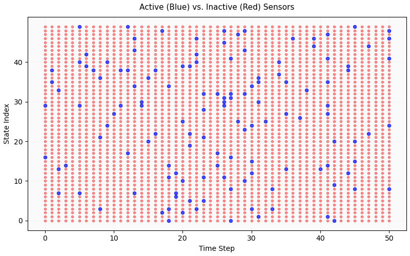
Figure 12 visualizes the number of active sensors at each time step. We consider the system with , where the sparsification parameter . Our result demonstrates that the system’s asymptotic stability can be achieved using measurements from a randomly selected subset (depicted in blue) of the state vector at each time step. Furthermore, the number of active sensors closely aligns with the expected sparsity, approximated by
References
- Distributed and localized model-predictive control–part i: synthesis and implementation. IEEE Transactions on Control of Network Systems 10 (2), pp. 1058–1068. Cited by: Large-scale power system.
- Mosek optimizer api for python. Version 9 (17), pp. 6–4. Cited by: Numerical Results.
- Feedback systems: an introduction for scientists and engineers. Princeton university press. Cited by: Introduction, Remark 3.
- Modern control systems. Cited by: Related work.
- Sparse feedback design in discrete-time linear systems. Automation and Remote Control 79, pp. 1175–1190. Cited by: Related work.
- On power control of grid-forming converters: modeling, controllability, and full-state feedback design. IEEE Transactions on Sustainable Energy 15 (1), pp. 68–80. Cited by: Grid-Forming Converter.
- Data sharing and compression for cooperative networked control. Advances in Neural Information Processing Systems 34, pp. 5947–5958. Cited by: Related work.
- CVX: matlab software for disciplined convex programming, version 2.0. Note: https://cvxr.com/cvx Cited by: Numerical Results.
- Distributed control design for spatially interconnected systems. IEEE Transactions on automatic control 48 (9), pp. 1478–1495. Cited by: Example of interconnected systems.
- Matrix computations. JHU press. Cited by: item 1.
- Homogeneous state feedback stabilization of homogenous systems. SIAM Journal on Control and Optimization 38 (4), pp. 1288–1308. Cited by: Randomized Sparsification Strategies, Main Results.
- Identification of spatially distributed discrete-time state-space models. IFAC Proceedings Volumes 45 (16), pp. 410–415. Cited by: Example of interconnected systems.
- Linear temporal logic for hybrid dynamical systems: characterizations and sufficient conditions. Nonlinear Analysis: Hybrid Systems 36, pp. 100865. Cited by: Conclusion.
- Linear systems theory. Princeton university press. Cited by: Introduction.
- Lyapunov stability. Control systems, robotics and automation 12, pp. 115. Cited by: Introduction.
- Stabilizing scheduling policies for networked control systems. IEEE Transactions on Control of Network Systems 7 (1), pp. 163–175. Cited by: Related work.
- Sparse feedback synthesis via the alternating direction method of multipliers. In 2012 American control conference (ACC), pp. 4765–4770. Cited by: Related work.
- Distributed identification and control of spatially interconnected systems with application to an actuated beam. Control engineering practice 54, pp. 104–116. Cited by: Example of interconnected systems.
- Sensor scheduling for linear systems: a covariance tracking approach. Automatica 136, pp. 110078. Cited by: Related work.
- Singular value assignment. SIAM Journal on Control and Optimization 48 (4), pp. 2388–2406. Cited by: Main Results, Proof of proposition 2.
- Interior-point polynomial algorithms in convex programming. SIAM. Cited by: item 2.
- Algorithms for joint sensor and control nodes selection in dynamic networks. Automatica 106, pp. 124–133. Cited by: Related work.
- Minimum input selection for structural controllability. IEEE Transactions on Automatic Control 60 (8), pp. 2163–2178. Cited by: Large-scale power system.
- An lmi approach to structured sparse feedback design in linear control systems. In 2013 European control conference (ECC), pp. 833–838. Cited by: Related work.
- Sparse feedback in linear control systems. Automation and Remote Control 75, pp. 2099–2111. Cited by: Related work.
- Temporal logic resilience for dynamical systems. arXiv preprint arXiv:2404.19223. Cited by: Conclusion.
- Necessary and sufficient conditions of asymptotic mean square stability for stochastic linear difference equations. Applied Mathematics Letters 10 (3), pp. 111–115. Cited by: Definition 1.
- Stabilizability of linear dynamical systems using sparse control inputs. IEEE Transactions on Automatic Control 68 (8), pp. 5014–5021. External Links: Document Cited by: Related work.
- Row/column sparse controller synthesis for network-based systems. In 2025 Information Science Frontier Forum and the Academic Conference on Information Security and Intelligent Control (ISF), pp. 80–83. Cited by: Related work.
- Stability theory of switched dynamical systems. Cited by: Remark 2.
- On efficient sensor scheduling for linear dynamical systems. Automatica 48 (10), pp. 2482–2493. Cited by: Related work.
- Gradient sparsification for communication-efficient distributed optimization. Advances in Neural Information Processing Systems 31. Cited by: Related work.
- The schur complement and its applications. Vol. 4, Springer Science & Business Media. Cited by: Proof of proposition 2.
- Sparse sensor selection for distributed systems: an l1-relaxation approach. Automatica 165, pp. 111670. Cited by: Randomized Sparsification Strategies.