跳到论文正文
W Papers独立论文阅读器 arXiv:2511.11974 论文正文 计算阅读时间 · 0%
引用这篇论文根据当前论文元数据生成,正式投稿前建议核对。


Estimating the critical threshold for stretched-out hyperbolic random connection models

Matthew Dickson111University of British Columbia, Department of Mathematics, Vancouver, BC, Canada, V6T 1Z2; Email: dickson@math.ubc.ca; https://orcid.org/0000-0002-8629-4796
Abstract

This paper examines the model-dependent asymptotic behaviour of the critical threshold intensity for stretched-out random connection models (RCMs) on hyperbolic spaces. The proof uses lace expansion arguments, but has notable qualitative differences to the Euclidean case in how it evaluates spectral radii. The result is applied to the Boolean disc RCM and a heat kernel RCM.

December 5, 2025

Mathematics Subject Classification (2020). Primary: 82B43; Secondary: 60G55, 43A90.

Keywords and phrases. Continuum percolation; random connection model; hyperbolic space; critical threshold; asymptotic behaviour; lace expansion

1 Introduction

Many percolative systems exhibit a phase transition: below some critical parameter value there exists no infinite connected component almost surely, and above the critical parameter there does exist an infinite connected component almost surely. Kesten proved in [kesten1980critical] that for Bernoulli bond percolation (BBP) on nearest-neighbour ℤ2\mathbb{Z}^{2} the critical edge probability pc=12p_{c}=\frac{1}{2}. Having such an exact answer for the critical value is atypical.

Estimates for the critical probability for spread-out Bernoulli bond percolation (BBP) on various graphs have been found in works such as [HarSla90, penrose1993spread, hofstadsakai2005critical, freiperkins2016lower, hong2023upper, spanos2024spread, hong2025lower]. Most relevant to this paper, [hofstadsakai2005critical] uses lace expansion results to examine spread-out BBP on ℤd\mathbb{Z}^{d} for d>6d>6. Amongst other results, they prove that if two vertices x,y∈ℤdx,y\in\mathbb{Z}^{d} share an edge independently with probability

p(2​L+1)d−1​𝟙​{‖x−y‖∞≤L},\frac{p}{\left(2L+1\right)^{d}-1}\mathds{1}\left\{\left\lVert x-y\right\rVert_{\infty}\leq L\right\}, (1.1)

then the critical probability obeys

pc=1+(U⋆2​(o)+12​∑n=3∞(n+1)​U⋆n​(o))​L−d+𝒪​(L−d−1),p_{\mathrm{c}}=1+\left(U^{\star 2}\left(o\right)+\frac{1}{2}\sum^{\infty}_{n=3}\left(n+1\right)U^{\star n}\left(o\right)\right)L^{-d}+\mathcal{O}\left(L^{-d-1}\right), (1.2)

as L→∞L\to\infty, where U:ℝd→[0,1]U\colon\mathbb{R}^{d}\to\left[0,1\right] is given by

U​(x):=2−d​𝟙​{‖x‖∞<1}U(x):=2^{-d}\mathds{1}\left\{\left\lVert x\right\rVert_{\infty}<1\right\} (1.3)

and U⋆n​(x)U^{\star n}\left(x\right) denotes the nn-fold convolution of UU in ℝd\mathbb{R}^{d}.

In this paper we will be concerned with approximating the critical threshold for stretched-out random connection models (RCMs) on the hyperbolic space ℍd{\mathbb{H}^{d}} (for d≥2d\geq 2). We will also be using a lace expansion approach (building upon the arguments in [HeyHofLasMat19] and [dickson2025expansion]), but will not require the full spread-out behaviour of [hofstadsakai2005critical], and the relevancy of terms in the asymptotics will differ from (1.2). The high-level proof description and the result will look similar to the argument in [dickson2025expansion] which dealt with RCMs on ℝd\mathbb{R}^{d} as d→∞d\to\infty, but as we shall see, the “easy” and “difficult” parts of the proof are transposed. The lace expansion component of the argument is now significantly easier because we can inherit the finiteness of the critical triangle diagram from the spherical transform argument in [dickson2024NonUniqueness] – no bootstrap argument is required. However, extracting the critical intensity, λc\lambda_{\mathrm{c}}, from the resulting Ornstein-Zernike equation is no longer as simple a matter as applying the (ℍd{\mathbb{H}^{d}}-analog of the) Fourier transform, and a more careful study of the L1→L1L^{1}\to L^{1} spectral radius of particular convolution operators is required.

Notation.

We write f=𝒪​(g)f=\mathcal{O}\left(g\right) to mean that lim sup|f/g|<∞\limsup\left\lvert\nicefrac{{f}}{{g}}\right\rvert<\infty, and write f=o​(g)f=o\left(g\right) or f≪gf\ll g to mean that limf/g=0\lim\nicefrac{{f}}{{g}}=0. By f∼gf\sim g we mean that limf/g=1\lim\nicefrac{{f}}{{g}}=1. Given a real-valued function ff, (f)+\left(f\right)_{+} is the positive part and (f)−\left(f\right)_{-} is the absolute value of the negative part. That is, (f)+:=12​(|f|+f)\left(f\right)_{+}:=\frac{1}{2}\left(\left\lvert f\right\rvert+f\right) and (f)−:=12​(|f|−f)\left(f\right)_{-}:=\frac{1}{2}\left(\left\lvert f\right\rvert-f\right). Given z∈ℂz\in\mathbb{C}, we write z¯\overline{z} for the complex conjugate of zz.

2 The Model and the Results

2.1 The Model

Hyperbolic space.

For d≥2d\geq 2, hyperbolic dd-space (denoted ℍd{\mathbb{H}^{d}}) is the unique simply connected dd-dimensional Riemannian manifold with constant sectional curvature −1-1. It can be convenient to describe ℍd{\mathbb{H}^{d}} using the Poincaré ball model (also called the conformal ball model). Let us consider the open Euclidean ball in ℝd\mathbb{R}^{d} with unit radius: 𝔹:={x∈ℝd:|x|<1}\mathbb{B}:=\left\{x\in\mathbb{R}^{d}\colon\left\lvert x\right\rvert<1\right\}. Then for each x∈𝔹x\in\mathbb{B} the hyperbolic metric on 𝔹\mathbb{B} assigns hyperbolic distance

distℍd​(x,o)=2​artanh​|x|,\mathrm{dist}_{{\mathbb{H}^{d}}}\left(x,o\right)=2\,\mathrm{artanh}\left\lvert x\right\rvert, (2.1)

where oo is the origin of ℝd\mathbb{R}^{d} and |⋅|\lvert\cdot\rvert is the Euclidean norm. The (hyperbolic-)isometries of 𝔹\mathbb{B} are then the Möbius transformations of 𝔹\mathbb{B}, and these can be used to extend this distance to any pair of points in 𝔹\mathbb{B}. For any Lebesgue measurable subset E⊂𝔹E\subset\mathbb{B}, the hyperbolic measure on 𝔹\mathbb{B} assigns mass

μ​(E):=∫E4(1−|x|2)2​dx.\mu\left(E\right):=\int_{E}\frac{4}{\left(1-\left\lvert x\right\rvert^{2}\right)^{2}}\mathrm{d}x. (2.2)

In particular, this measure is preserved by the (hyperbolic-)isometries of 𝔹\mathbb{B}.

Also note that for a μ\mu-integrable function f:ℍd→ℝf\colon{\mathbb{H}^{d}}\to\mathbb{R} for which there exists g:ℝ≥0→ℝg\colon\mathbb{R}_{\geq 0}\to\mathbb{R} such that f​(x)=g​(distℍd​(x,o))f(x)=g\left(\mathrm{dist}_{{\mathbb{H}^{d}}}\left(x,o\right)\right),

∫ℍdf​(x)​μ​(d​x)=𝔖d−1​∫0∞g​(r)​(sinh⁡r)d−1​dr,\int_{\mathbb{H}^{d}}f(x)\mu\left(\mathrm{d}x\right)=\mathfrak{S}_{d-1}\int^{\infty}_{0}g(r)\left(\sinh r\right)^{d-1}\mathrm{d}r, (2.3)

where 𝔖d−1:=2​πd2/Γ​(d2)\mathfrak{S}_{d-1}:=\nicefrac{{2\pi^{\frac{d}{2}}}}{{\Gamma\left(\frac{d}{2}\right)}} equals the ℝd−1\mathbb{R}^{d-1}-Lebesgue measure of the Euclidean unit radius sphere (i.e. 𝕊d−1\mathbb{S}^{d-1}) in ℝd\mathbb{R}^{d}.

Random connection model.

Given λ≥0\lambda\geq 0 let the vertex set of the RCM, η\eta, be distributed as a Poisson point process on ℍd{\mathbb{H}^{d}} with intensity measure λ​μ\lambda\mu, where μ\mu is the hyperbolic measure on ℍd{\mathbb{H}^{d}}. Given a measurable adjacency function φ:ℝ≥0→[0,1]\varphi\colon\mathbb{R}_{\geq 0}\to\left[0,1\right], for each pair of vertices in η\eta (say, {x,y}\left\{x,y\right\}), assign an edge independently of everything else with probability

φ​(distℍd​(x,y)).\varphi\left(\mathrm{dist}_{{\mathbb{H}^{d}}}\left(x,y\right)\right). (2.4)

We will sometimes write φ​(x,y):=φ​(distℍd​(x,y))\varphi\left(x,y\right):=\varphi\left(\mathrm{dist}_{{\mathbb{H}^{d}}}\left(x,y\right)\right). The overloading of notation should cause minimal confusion. Note that since hyperbolic translations generate hyperbolic rotations (see for example [martin2012foundations, Exercise 29.13]), this is no great restriction on the family of adjacency functions we can consider if we want some sort of transitivity in the model. If xx and yy share an edge, we say xx and yy are adjacent, and write x∼yx\sim y. The configuration of the vertex set and the edge set is then notated with ξ\xi. We will also require Palm-type versions of η\eta and ξ\xi. Given a finite set {x1,…,xk}⊂ℍd\left\{x_{1},\ldots,x_{k}\right\}\subset{\mathbb{H}^{d}}, we can define the augmented vertex set ηx1,…,xk=η∪{x1,…,xk}\eta^{x_{1},\ldots,x_{k}}=\eta\cup\left\{x_{1},\ldots,x_{k}\right\} and define the augmented configuration ξx1,…,xk\xi^{x_{1},\ldots,x_{k}} by using the augmented vertex set and including edges between any two vertices in ηx1,…,xk\eta^{x_{1},\ldots,x_{k}} independently with probability given by φ\varphi. The full details of this construction can be found in [HeyHofLasMat19].
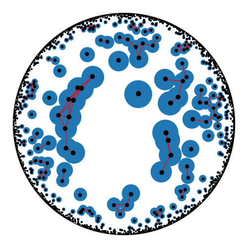
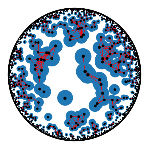
Refer to caption
(a) λ=2.0\lambda=2.0
Refer to caption
(b) λ=4.0\lambda=4.0
Figure 1: Simulations of the RCM on ℍ2{\mathbb{H}^{2}} (represented with the Poincaré ball model) with adjacency function φ​(r)=𝟙​{r<r0}\varphi\left(r\right)=\mathds{1}\left\{r<r_{0}\right\} where r0=2​a​r​s​i​n​h​(12​π)≈0.557r_{0}=2\mathrm{arsinh}\left(\frac{1}{2\sqrt{\pi}}\right)\approx 0.557 is the radius of the unit μ\mu-volume disc. The blue region is the union of hyperbolic radius 12​r0\frac{1}{2}r_{0} discs centred on each vertex.

Given an index L>0L>0, let φL\varphi_{L} be an adjacency function. In the examples we consider in Theorems 2.2 and 2.4, and in Assumption A, we shall come to view models with larger LL as being more ‘stretched-out’ in that longer edges beome more likely. This adjacency function and an intensity λ\lambda will define a RCM on ℍd{\mathbb{H}^{d}}. Let ℙλ,L\mathbb{P}_{\lambda,L} and 𝔼λ,L\mathbb{E}_{\lambda,L} denote the probability and expectation associated with ξ\xi in the RCM on ℍd{\mathbb{H}^{d}} with intensity λ\lambda and adjacency function φL\varphi_{L}. The assumptions required for our results will impose constraints on the family of functions {φL}L>0\left\{\varphi_{L}\right\}_{L>0} we can consider.

Given two distinct vertices x,y∈ℍdx,y\in{\mathbb{H}^{d}}, we say xx is connected to yy in ξx,y\xi^{x,y} (written x⟷y​ in ​ξx,yx\longleftrightarrow y\textrm{ in }\xi^{x,y}) if x=yx=y or there exists a finite sequence of edges in ξx,y\xi^{x,y} leading from xx to yy. This leads to defining the useful two-point function:

τλ,L(x,y):=ℙλ,L(x⟷y in ξx,y).\tau_{\lambda,L}\left(x,y\right):=\mathbb{P}_{\lambda,L}\left(x\longleftrightarrow y\textrm{ in }\xi^{x,y}\right). (2.5)

Critical Intensity.

Our main question of these hyperbolic random connection models regards the existence of an infinite connected component (a cluster) in the resulting random graph. Let

λc\displaystyle\lambda_{\mathrm{c}} :=inf{λ≥0:the RCM on ​ℍd​ with intensity ​λ​ has an infinite cluster a.s},\displaystyle:=\inf\left\{\lambda\geq 0\colon\text{the RCM on }{\mathbb{H}^{d}}\text{ with intensity }\lambda\text{ has an infinite cluster a.s}\right\}, (2.6)
λu\displaystyle\lambda_{u} :=inf{λ≥0:the RCM on ​ℍd​ with intensity ​λ​ has a unique infinite cluster a.s}.\displaystyle:=\inf\left\{\lambda\geq 0\colon\text{the RCM on }{\mathbb{H}^{d}}\text{ with intensity }\lambda\text{ has a unique infinite cluster a.s}\right\}. (2.7)

For RCMs on ℝd\mathbb{R}^{d}, [MeeRoy96] proves that the analogous quantities are in fact equal, and [chebunin2024uniqueness] proves that this equality survives even if the vertices are randomly and independently assigned ‘marks’ that can change the adjacency probabilities (with some conditions). However, [tykesson2007number] proves that for the Boolean disc RCM on ℍ2{\mathbb{H}^{2}} (see Definition 2.1),

0<λc<λu<∞.0<\lambda_{\mathrm{c}}<\lambda_{u}<\infty. (2.8)

In fact [tykesson2007number] proves that if the radius of the Boolean discs is sufficiently large (depending on the dimension dd), λc<λu\lambda_{\mathrm{c}}<\lambda_{u} for the Boolean disc RCM on ℍd{\mathbb{H}^{d}} for any d≥2d\geq 2. This latter result is generalised in [dickson2024NonUniqueness] to show that λc<λu\lambda_{\mathrm{c}}<\lambda_{u} for many ‘stretched-out’ RCMs on ℍd{\mathbb{H}^{d}}, even when marks are added to the vertices.

When we have a family of RCMs determined by the family of adjacency functions {φL}L>0\left\{\varphi_{L}\right\}_{L>0}, we will naturally have λc=λc​(L)\lambda_{\mathrm{c}}=\lambda_{\mathrm{c}}(L). In this paper we aim to describe the asymptotics of λc​(L)\lambda_{\mathrm{c}}(L) as L→∞L\to\infty.

2.2 Results

Before introducing the most general form of our result, we present two concrete examples of it in action: the heat kernel RCM on ℍ3{\mathbb{H}^{3}}, and the Boolean disc RCM on ℍd{\mathbb{H}^{d}} (for any d≥2d\geq 2).

Definition 2.1 (Boolean disc RCM).

The Boolean disc RCM is defined by having the adjacency function

φL​(r)=𝟙​{r<L}.\varphi_{L}(r)=\mathds{1}\left\{r<L\right\}. (2.9)

By 𝔖d−1\mathfrak{S}_{d-1} we denote the ℝd−1\mathbb{R}^{d-1}-Lebesgue measure of the Euclidean unit radius sphere (i.e. 𝕊d−1\mathbb{S}^{d-1}) in ℝd\mathbb{R}^{d}, and note we will let BL​(o)B_{L}\left(o\right) denote the hyperbolic radius LL ball centred on o∈ℍdo\in{\mathbb{H}^{d}}. Therefore μ​(BL​(o))\mu\left(B_{L}\left(o\right)\right) denotes the hyperbolic measure of the hyperbolic radius LL ball.

Theorem 2.2.

For the Boolean disc RCM, as L→∞L\to\infty

μ​(BL​(o))​λc​(L)=1+𝔖d−2𝔖d−1​2d+2d−1​e−12​(d−1)​L+o​(e−12​(d−1)​L).\mu\left(B_{L}(o)\right)\lambda_{c}(L)=1+\frac{\mathfrak{S}_{d-2}}{\mathfrak{S}_{d-1}}\frac{2^{d+2}}{d-1}\text{e}^{-\frac{1}{2}\left(d-1\right)L}+o\left(\text{e}^{-\frac{1}{2}\left(d-1\right)L}\right). (2.10)

Therefore

λc​(L)=(d−1)​2d−1𝔖d−1​e−(d−1)​L​(1+(1+o​(1))​{16π​e−12​L:d=28​e−L:d=31283​π​e−32​L:d=432​e−2​L:d=5(d−1)2d−3​e−2​L:d≥6).\lambda_{c}(L)=\frac{\left(d-1\right)2^{d-1}}{\mathfrak{S}_{d-1}}\text{e}^{-\left(d-1\right)L}\left(1+\left(1+o\left(1\right)\right)\begin{cases}\frac{16}{\pi}\text{e}^{-\frac{1}{2}L}&\colon d=2\\ 8\text{e}^{-L}&\colon d=3\\ \frac{128}{3\pi}\text{e}^{-\frac{3}{2}L}&\colon d=4\\ 32\text{e}^{-2L}&\colon d=5\\ \frac{\left(d-1\right)^{2}}{d-3}\text{e}^{-2L}&\colon d\geq 6\end{cases}\right). (2.11)

The order of the error term in (2.11) becomes fixed for d≥5d\geq 5 because the correction term for μ​(BL​(o))\mu\left(B_{L}(o)\right) becomes relevant for d=5d=5 and dominant for d≥6d\geq 6. There is no indication that this is related to d=6d=6 being the upper critical dimension for Euclidean percolation models.

Definition 2.3 (Heat Kernel RCM on ℍ3{\mathbb{H}^{3}}).

Note that the heat kernel K3:ℝ>0×ℍ3×ℍ3→ℝ>0K_{3}\colon\mathbb{R}_{>0}\times{\mathbb{H}^{3}}\times{\mathbb{H}^{3}}\to\mathbb{R}_{>0} is given by

K3​(t,x,y)=1(2​π​t)32​distℍ3​(x,y)sinh⁡distℍ3​(x,y)​exp⁡(−t2−distℍ3​(x,y)22​t),K_{3}\left(t,x,y\right)=\frac{1}{\left(2\pi t\right)^{\frac{3}{2}}}\frac{\mathrm{dist}_{{\mathbb{H}^{3}}}\left(x,y\right)}{\sinh\mathrm{dist}_{{\mathbb{H}^{3}}}\left(x,y\right)}\exp\left(-\frac{t}{2}-\frac{\mathrm{dist}_{{\mathbb{H}^{3}}}\left(x,y\right)^{2}}{2t}\right), (2.12)

see [davies1988heat]. Note (or see in the proof of Lemma 8.6) that ∫ℍ3K3​(t,x,y)​μ​(d​x)=1\int_{\mathbb{H}^{3}}K_{3}\left(t,x,y\right)\mu\left(\mathrm{d}x\right)=1 for all t>0t>0 and y∈ℍ3y\in{\mathbb{H}^{3}}. Now let 0<𝒜L≤(2​π​L)32​e12​L0<\mathcal{A}_{L}\leq\left(2\pi L\right)^{\frac{3}{2}}\text{e}^{\frac{1}{2}L} for all L>0L>0. The heat kernel RCM on ℍ3{\mathbb{H}^{3}} is defined by having the adjacency function

φL​(r)=𝒜L(2​π​L)32​rsinh⁡r​exp⁡(−12​L−12​L​r2)\varphi_{L}\left(r\right)=\frac{\mathcal{A}_{L}}{\left(2\pi L\right)^{\frac{3}{2}}}\frac{r}{\sinh r}\exp\left(-\frac{1}{2}L-\frac{1}{2L}r^{2}\right) (2.13)

for all L>0L>0. One can think of this as a hyperbolic analog of the RCM on ℝd\mathbb{R}^{d} with a Gaussian adjacency function with variance parameter LL and amplitude 𝒜L\mathcal{A}_{L}. Like the Gaussian function on ℝd\mathbb{R}^{d}, this heat kernel satisfies the semi-group property, which will make it convenient to evaluate convolutions. The sole purpose of having 𝒜L≤(2​π​L)32​e12​L\mathcal{A}_{L}\leq\left(2\pi L\right)^{\frac{3}{2}}\text{e}^{\frac{1}{2}L} is to ensure φL​(x,y)∈[0,1]\varphi_{L}\left(x,y\right)\in\left[0,1\right] for all L>0L>0 and x,y∈ℍ3x,y\in{\mathbb{H}^{3}}. We have restricted to d=3d=3 so that the heat kernel takes its most simple and explicit form.

Theorem 2.4.

Consider the heat kernel RCM on ℍ3{\mathbb{H}^{3}}. As L→∞L\to\infty,

𝒜L​λc​(L)=1+𝒜L(6​π)32​L−32​e−32​L+32​𝒜L(8​π)32​L−32​e−2​L+𝒪​(𝒜L​L−32​e−52​L+𝒜L2​L−92​e−52​L).\mathcal{A}_{L}\lambda_{\mathrm{c}}(L)=1+\frac{\mathcal{A}_{L}}{\left(6\pi\right)^{\frac{3}{2}}}L^{-\frac{3}{2}}\text{e}^{-\frac{3}{2}L}+\frac{3}{2}\frac{\mathcal{A}_{L}}{\left(8\pi\right)^{\frac{3}{2}}}L^{-\frac{3}{2}}\text{e}^{-2L}+\mathcal{O}\left(\mathcal{A}_{L}L^{-\frac{3}{2}}\text{e}^{-\frac{5}{2}L}+\mathcal{A}_{L}^{2}L^{-\frac{9}{2}}\text{e}^{-\frac{5}{2}L}\right). (2.14)

In particular, if φL​(o,o)=1\varphi_{L}(o,o)=1 for all L>0L>0 (i.e. 𝒜L=(2​π​L)32​e12​L\mathcal{A}_{L}=\left(2\pi L\right)^{\frac{3}{2}}\text{e}^{\frac{1}{2}L}) then as L→∞L\to\infty

λc​(L)=1(2​π)32​L−32​e−12​L​(1+13​3​e−L+316​e−32​L+𝒪​(L−32​e−32​L)).\lambda_{\mathrm{c}}(L)=\frac{1}{\left(2\pi\right)^{\frac{3}{2}}}L^{-\frac{3}{2}}\text{e}^{-\frac{1}{2}L}\left(1+\frac{1}{3\sqrt{3}}\text{e}^{-L}+\frac{3}{16}\text{e}^{-\frac{3}{2}L}+\mathcal{O}\left(L^{-\frac{3}{2}}\text{e}^{-\frac{3}{2}L}\right)\right). (2.15)

Note that which of the two last error terms in (2.14) is dominant depends upon the order of the amplitude term 𝒜L\mathcal{A}_{L}: 𝒜L​L−32​e−52​L\mathcal{A}_{L}L^{-\frac{3}{2}}\text{e}^{-\frac{5}{2}L} is dominant if 𝒜L≪L3\mathcal{A}_{L}\ll L^{3}, while 𝒜L2​L−92​e−52​L\mathcal{A}_{L}^{2}L^{-\frac{9}{2}}\text{e}^{-\frac{5}{2}L} is dominant if 𝒜L≫L3\mathcal{A}_{L}\gg L^{3}.

While the above two theorems are for specific models, the following proposition provides a result for a wide class of RCM on ℍd{\mathbb{H}^{d}}. We only require the following assumption.

Assumption A.

We require that the family of adjacency functions {φL}L>0\left\{\varphi_{L}\right\}_{L>0} satisfies:

  1. (A.1)

    for all L>0L>0,

    0<∫0∞φL​(r)​exp⁡((d−1)​r)​dr<∞,0<\int^{\infty}_{0}\varphi_{L}\left(r\right)\exp\left(\left(d-1\right)r\right)\mathrm{d}r<\infty, (2.16)
  2. (A.2)

    for all R>0R>0,

    limL→∞∫0RφL​(r)​(sinh⁡r)d−1​dr∫0∞φL​(r)​(sinh⁡r)d−1​dr=0.\lim_{L\to\infty}\frac{\int^{R}_{0}\varphi_{L}\left(r\right)\left(\sinh r\right)^{d-1}\mathrm{d}r}{\int^{\infty}_{0}\varphi_{L}\left(r\right)\left(\sinh r\right)^{d-1}\mathrm{d}r}=0. (2.17)
Proposition 2.5.

Suppose {φL}L>0\left\{\varphi_{L}\right\}_{L>0} satisfies Assumption A. Then as L→∞L\to\infty,

λc​(L)​∫ℍdφL​(x,o)​μ​(d​x)=1+o​(1).\lambda_{\mathrm{c}}(L)\int_{\mathbb{H}^{d}}\varphi_{L}\left(x,o\right)\mu\left(\mathrm{d}x\right)=1+o\left(1\right). (2.18)
Remark 2.6.

Mecke’s formula (see Section 3) implies that λc​(L)​∫ℍdφL​(x,o)​μ​(d​x)\lambda_{\mathrm{c}}(L)\int_{\mathbb{H}^{d}}\varphi_{L}\left(x,o\right)\mu\left(\mathrm{d}x\right) is equal to the expected degree of a typical vertex in the RCM. Similarly, the left hand sides of (2.10) and (2.14) are equal to the expected degree of a typical vertex in their respective RCMs. We can therefore view Theorems 2.2 and 2.4 and Proposition 2.5 as results on the expected degree of a typical vertex in each RCM approaching 11 as L→∞L\to\infty.

Remark 2.7.

Here are a few remarks on Assumption A.

  1. i)

    Observe that Assumption (A.1) with Mecke’s formula implies that 0<𝔼λ,L​[deg⁡o]<∞0<\mathbb{E}_{\lambda,L}\left[\deg{o}\right]<\infty for all λ>0\lambda>0 and L>L0L>L_{0}. If instead we had ∫ℍdφL​(x,o)​μ​(d​x)=∞\int_{\mathbb{H}^{d}}\varphi_{L}\left(x,o\right)\mu\left(\mathrm{d}x\right)=\infty for some LL, then 𝔼λ,L​[deg⁡o]=∞\mathbb{E}_{\lambda,L}\left[\deg{o}\right]=\infty for all λ>0\lambda>0 and λc​(L)=0\lambda_{\mathrm{c}}(L)=0. On the other hand, if ∫ℍdφL​(x,o)​μ​(d​x)=0\int_{\mathbb{H}^{d}}\varphi_{L}\left(x,o\right)\mu\left(\mathrm{d}x\right)=0, then there are almost surely no edges at all and λc​(L)=∞\lambda_{\mathrm{c}}(L)=\infty. This assumption therefore allows estimating λc\lambda_{\mathrm{c}} to be an interesting question.

  2. ii)

    In the context of Assumption A and Proposition 2.5 LL is just an index for a family of adjacency functions, and therefore Assumption (A.1) can be weakened to only hold for L>L0L>L_{0} for some L0L_{0}. There are some places in the argument where having LL “sufficiently large” is important for an independent reason, and having this assumption hold for all L>0L>0 makes it easier to identify these places.

  3. iii)

    If one specifically considers adjacency functions of the form φL​(r)=φ​(1L​r)\varphi_{L}\left(r\right)=\varphi\left(\frac{1}{L}r\right) for some fixed reference adjacency function φ\varphi, then [dickson2024NonUniqueness, Lemma A.3] proves that Assumption (A.2) is satisfied as long as ∫0∞φ​(r)​dr>0\int^{\infty}_{0}\varphi(r)\mathrm{d}r>0. Assumption (A.1) is then also satisfied as long as φ​(r)\varphi(r) is not 0 almost everywhere, and decays faster than exponentially as r→∞r\to\infty. Increasing the parameter LL in this case corresponds to increasing the typical length scale of edges of the RCM in ℍd{\mathbb{H}^{d}}. Therefore (up to an overall scaling of the intensity λ\lambda) increasing LL corresponds to increasing the (negative) curvature of the ℍd{\mathbb{H}^{d}} space. One may then interpret the L→∞L\to\infty regime in this case as a ‘high curvature’ regime.

Proposition 2.5 is actually a simplification of Theorem 7.5 later in this paper. While that result also requires Assumption A, it provides more detail to the error term in (2.18). In particular, a bound on the o​(1)o\left(1\right) term is provided that depends explicitly on the adjacency function φL\varphi_{L}. The extra precision of Theorem 7.5 is required to derive the asymptotics in Theorems 2.2 and 2.4.

2.3 Background and Discussion

In this paper we give ourselves some flexibility in only asking for an asymptotic expression for the critical threshold in some perturbative regime, rather than asking for the exact value. This approach has been taken many times before. If we let GLG_{L} be the graph on ℤd\mathbb{Z}^{d} (with d≥2d\geq 2) with edge set connecting vertices x,y∈ℤdx,y\in\mathbb{Z}^{d} such that ‖x−y‖∞≤L\left\lVert x-y\right\rVert_{\infty}\leq L, then [penrose1993spread] proves that the critical probability satisfies

pc​(L)​deg⁡GL=1+o​(1)p_{\mathrm{c}}(L)\deg{G_{L}}=1+o\left(1\right) (2.19)

as L→∞L\to\infty. The quantity pc​deg⁡GLp_{\mathrm{c}}\deg{G_{L}} can also be interpreted as the expected degree of the percolation sub-graph at criticality – naturally drawing comparison to (2.18). In [spanos2024spread], the behaviour (2.19) is proven for such spread-out versions of BBP on transitive graphs with superlinear polynomial growth.

The order of the error in (2.19) has been refined for a number of cases. [freiperkins2016lower] and [hong2023upper] compare BBP to the ‘SIR epidemic’ model to find matching lower and upper bounds for the error for spread-out BBP on ℤd\mathbb{Z}^{d} for d=2,3d=2,3, while [hong2025lower] uses a similar approach to find a lower bound for d=4,5,6d=4,5,6.

Such more precise estimates on the expected degree at criticality have also been found for spread-out BBP on ℤd\mathbb{Z}^{d} for d>6d>6 in [hofstadsakai2005critical] – see (1.2) above. This work is one of many that have used lace expansion techniques to arrive at estimates for pcp_{\mathrm{c}}. For example, [HofSla05] uses the lace expansion to get asymptotics for pcp_{\mathrm{c}} for BBP on nearest-neighbour ℤd\mathbb{Z}^{d} and the dd-dimensional hypercube as d→∞d\to\infty. In [HeyMat19b] asymptotics for the critical probability of site percolation on nearest-neighbour ℤd\mathbb{Z}^{d} as d→∞d\to\infty are similarly proven.

For RCMs with background space ℝd\mathbb{R}^{d}, [dickson2025expansion] uses lace expansion results from [HeyHofLasMat19] to derive asymptotics for the critical intensity λc\lambda_{\mathrm{c}} as d→∞d\to\infty. In particular, if φ=φd\varphi=\varphi_{d} is given by a Gaussian function with total mass 11 and variance σ2​(d)\sigma^{2}(d) such that lim infd→∞φ​(o,o)12>0\liminf_{d\to\infty}\varphi(o,o)^{\frac{1}{2}}>0, then

λc​(d)=1+(6​π​σ2)−d2+32​(8​π​σ2)−d2+2​(10​π​σ2)−d2+𝒪​((12​π​σ2)−d2)\lambda_{\mathrm{c}}(d)=1+\left(6\pi\sigma^{2}\right)^{-\frac{d}{2}}+\frac{3}{2}\left(8\pi\sigma^{2}\right)^{-\frac{d}{2}}+2\left(10\pi\sigma^{2}\right)^{-\frac{d}{2}}+\mathcal{O}\left(\left(12\pi\sigma^{2}\right)^{-\frac{d}{2}}\right) (2.20)

as d→∞d\to\infty.

Before we compare the result in this paper to results regarding RCMs on ℝd\mathbb{R}^{d}, we should highlight a difference between λc\lambda_{\mathrm{c}} for ℝd\mathbb{R}^{d}-RCMs and λc\lambda_{\mathrm{c}} for ℍd{\mathbb{H}^{d}}-RCMs. Recall that τλ,L​(x,y)\tau_{\lambda,L}(x,y) is the two-point function that returns the probability that xx is connected to yy in the RCM. We can use this two-point function to define a two-point convolution operator 𝒯λ,L\mathcal{T}_{\lambda,L} (for details, see Section 3). The operator norm of this operator can depend upon the spaces it is defined on: for p∈[1,∞]p\in\left[1,\infty\right], ‖𝒯λ,L‖p→p\left\lVert\mathcal{T}_{\lambda,L}\right\rVert_{p\to p} denotes the operator norm of 𝒯λ,L:Lp→Lp\mathcal{T}_{\lambda,L}\colon L^{p}\to L^{p}. We can then define

λ2→2​(L)\displaystyle\lambda_{2\to 2}(L) :=inf{λ≥0:‖𝒯λ,L‖2→2=∞},\displaystyle:=\inf\left\{\lambda\geq 0\colon\left\lVert\mathcal{T}_{\lambda,L}\right\rVert_{2\to 2}=\infty\right\}, (2.21)
λ1→1​(L)\displaystyle\lambda_{1\to 1}(L) :=inf{λ≥0:‖𝒯λ,L‖1→1=∞}.\displaystyle:=\inf\left\{\lambda\geq 0\colon\left\lVert\mathcal{T}_{\lambda,L}\right\rVert_{1\to 1}=\infty\right\}. (2.22)

For ℝd\mathbb{R}^{d}-RCMs one can use the Fourier transform to show λ2→2=λ1→1\lambda_{2\to 2}=\lambda_{1\to 1}. On the other hand, [dickson2024NonUniqueness] shows that for ℍd{\mathbb{H}^{d}}-RCMs satisfying Assumption (A.2) with sufficiently large LL, we have λ2→2​(L)>λ1→1​(L)\lambda_{2\to 2}(L)>\lambda_{1\to 1}(L). For ℝd\mathbb{R}^{d}-RCMs, [Mee95] proved that λc=λ1→1\lambda_{\mathrm{c}}=\lambda_{1\to 1} while [dickson2024NonUniqueness] proved this same equality for ℍd{\mathbb{H}^{d}}-RCMs with sufficiently large LL.

While the central result and high-level proof outline of this paper strongly resembles the central result of [dickson2025expansion], it is notable the inequality λ2→2>λ1→1\lambda_{2\to 2}>\lambda_{1\to 1} means that the difficulties are reversed. In the ℝd\mathbb{R}^{d}-RCM case, the derivation of the lace expansion was challenging because a sophisticated bootstrap argument was required to extend a property from λ<λ2→2\lambda<\lambda_{2\to 2} to λ≤λ2→2\lambda\leq\lambda_{2\to 2}. Once the uniform convergence to an Ornstein-Zernike equation was established, it was relatively clear (if involved) to expand λ2→2\lambda_{2\to 2} because the Fourier transform diagonalises the equation. On the other hand, deriving the lace expansion Ornstein-Zernike equation for RCMs on ℍd{\mathbb{H}^{d}} is simple for λ≤λ1→1\lambda\leq\lambda_{1\to 1}, because the triangle condition is already established in [dickson2024NonUniqueness]. However because we want an expansion for λ1→1\lambda_{1\to 1} – and not λ2→2\lambda_{2\to 2} – the spherical transform does not give the shortcut that the Fourier transform does in ℝd\mathbb{R}^{d}.

It should, nevertheless, be possible to derive an expansion for λ2→2\lambda_{2\to 2} in this ℍd{\mathbb{H}^{d}} case. Like for the ℝd\mathbb{R}^{d} case, the main challenge is the derivation of the Ornstein-Zernike equation on the whole domain λ≤λ2→2\lambda\leq\lambda_{2\to 2}. Once this is achieved, the spherical transform can then be used to extract λ2→2\lambda_{2\to 2}. While the value λ2→2\lambda_{2\to 2} currently has less probabilistic interest than the λc\lambda_{\mathrm{c}} critical intensity, [dickson2024NonUniqueness] shows that it provides a lower bound for the uniqueness threshold λu\lambda_{\mathrm{u}}.

Observe that the corrections to the leading term for both the heat kernel RCM on ℍ3{\mathbb{H}^{3}} and the Boolean disc RCM on ℍd{\mathbb{H}^{d}} are exponentially small in LL, while the corrections to the leading term for spread-out BBP on ℤd\mathbb{Z}^{d} for d>6d>6 (see [hofstadsakai2005critical] or (1.2)) follow a power law. This exponential decay is not a consequence of Theorem 2.5, because one can always ‘slow down’ LL and Assumption A will still hold. There would need to be a more concrete map between RCMs on ℝd\mathbb{R}^{d} to RCMs on ℍd{\mathbb{H}^{d}} for a theorem along the lines of “corrections to the leading term for RCMs on ℍd{\mathbb{H}^{d}} are smaller than corrections to the leading term for RCMs on ℝd\mathbb{R}^{d}” to be made. The closest we have to that here is comparing (1.2) to Theorem 2.2, which suggests there may be something to explore here.

Throughout this paper we have fixed the curvature of ℍd{\mathbb{H}^{d}} to be −1-1. It would be an interesting avenue of investigation to see how the approximations of λc\lambda_{\mathrm{c}} behave as the curvature of ℍd{\mathbb{H}^{d}} approaches 0. Does the approximation approach something meaningful for λc\lambda_{\mathrm{c}} of an RCM on ℝd\mathbb{R}^{d}? For 2≤d≤62\leq d\leq 6, there is good reason to believe the answer is no. This is because the lace expansion for RCMs on ℝd\mathbb{R}^{d} (fundamentally the same as the lace expansion on ℍd{\mathbb{H}^{d}}) should not converge for d≤6d\leq 6. It may be that the hidden constants in o​(1)o\left(1\right) in Proposition 2.5 grow and eventually diverge as the curvature vanishes.

2.4 Outline of the Paper and the Argument

In Section 3 we establish some preliminary results: specifically we recall Mecke’s formula (which we use many times throughout the paper) and provide some simple properties of the operators we are considering in this paper. Note that in Theorem 3.4 we also recall a result from [dickson2024NonUniqueness] that will be crucial to our argument – in particular we already have a bound on the triangle diagram at λc\lambda_{\mathrm{c}}.

Theorems 2.2 and 2.4 and Proposition 2.5 are all corollaries of Theorem 7.5. Sections 4 to 7 lay the ground-work for and culminate in a proof of Theorem 7.5. In Section 4 we provide the lace expansion for the hyperbolic RCM for λ≤λc\lambda\leq\lambda_{\mathrm{c}}, leading to Proposition 4.4. This proceeds very similarly to the derivation of the lace expansion for RCMs on ℝd\mathbb{R}^{d} (see [HeyHofLasMat19, DicHey2022triangle]), with a major simplification in the fact that we already have the bound on the triangle diagram from [dickson2024NonUniqueness].

We then outline how the Ornstein-Zernike equation resulting from the lace expansion can be used to extract the value of λc\lambda_{\mathrm{c}} in Section 5. In particular, this involves understanding the L1→L1L^{1}\to L^{1} spectral radius of the sum of the adjacency operator and the lace expansion coefficient operator.

The issue now is that the lace expansion coefficient operator is an implicit object defined via the model. In Section 6 we replicate the arguments of [dickson2025expansion] to obtain an approximation of these lace expansion coefficients in terms of the adjacency function. The main difference between the argument in [dickson2025expansion] and the argument here is that on ℍd{\mathbb{H}^{d}} we don’t have the usual Fourier transform and the associated tools. We do, however, have access to the spherical transform – an analog of the Fourier transform for symmetric spaces. This plays a crucial role in [dickson2024NonUniqueness], and we use it here to prove that the intermediate results in [dickson2025expansion] that made use of the Fourier transform also hold in our case.

In Section 7 we use this approximation of the lace expansion coefficients to get an approximation of the L1→L1L^{1}\to L^{1} spectral radius in terms of λc\lambda_{\mathrm{c}} and the adjacency function. This gives λc\lambda_{\mathrm{c}} as the solution of a polynomial equation (of which one term is only known asymptotically), and we use this to get the asymptotic behaviour of λc\lambda_{\mathrm{c}}. This completes the proof of Theorem 7.5. Proposition 2.5 then follows directly.

In Section 8 we show how the terms in Theorem 7.5 can be simplified in three cases: when we restrict to what we call ‘non-negative definite’ RCMs, when we restrict to the heat kernel model (leading to Theorem 2.4), and when we restrict to the Boolean disc RCM (leading to Theorem 2.2).

Appendix A contains the proofs for most of the preliminary lemmas in Section 3. In Appendix B we prove an elementary property of the spherical transform that applies for the functions we are considering and is used multiple times – specifically that the range of the transformed functions are subsets of the real line. In Appendix C we give some standard properties of hyperbolic triangles which are used in Section 8.3 to study the Boolean disc RCM.

3 Preliminaries

Mecke’s Formula.

Mecke’s formula gives us a way to formulate some expectations of integrals (or sums) as integrals of expectations. Given m∈ℕm\in\mathbb{N} and a measurable function f=f​(ξ,x1,…,xm)∈ℝ≥0f=f\left(\xi,x_{1},\ldots,x_{m}\right)\in\mathbb{R}_{\geq 0},

𝔼λ,L​[∑(x1,…,xm)∈η(m)f​(ξ,x1,…,xm)]=λm​∫(ℍd)m𝔼λ,L​[f​(ξx1,…,xm,x1,…,xm)]​μ​(d​x1)​…​μ​(d​xm),\mathbb{E}_{\lambda,L}\left[\sum_{\left(x_{1},\ldots,x_{m}\right)\in\eta^{(m)}}f\left(\xi,x_{1},\ldots,x_{m}\right)\right]\\ =\lambda^{m}\int_{\left({\mathbb{H}^{d}}\right)^{m}}\mathbb{E}_{\lambda,L}\left[f\left(\xi^{x_{1},\ldots,x_{m}},x_{1},\ldots,x_{m}\right)\right]\mu\left(\mathrm{d}x_{1}\right)\ldots\mu\left(\mathrm{d}x_{m}\right), (3.1)

where η(m):={(y1,…,ym)∈ηm:xi≠xj​ for ​i≠j}\eta^{(m)}:=\left\{\left(y_{1},\ldots,y_{m}\right)\in\eta^{m}\colon x_{i}\neq x_{j}\text{ for }i\neq j\right\}. For details, see [LasPen17, §4].

Notable examples of the use of Mecke’s formula are to get expressions for the expected degree and expected cluster size of a RCM. Let deg⁡o:=#​{y∈η:y∼o​ in ​ξo}\deg{o}:=\#\left\{y\in\eta\colon y\sim o\textrm{ in }\xi^{o}\right\} and 𝒞​(o):={o}∪{y∈η:y⟷o​ in ​ξo}\mathscr{C}\left(o\right):=\left\{o\right\}\cup\left\{y\in\eta\colon y\longleftrightarrow o\textrm{ in }\xi^{o}\right\}. Then Mecke’s formula implies

𝔼λ,L​[deg⁡o]=𝔼λ,L​[∑x∈η𝟙​{x∼o​ in ​ξo}]\displaystyle\mathbb{E}_{\lambda,L}\left[\deg{o}\right]=\mathbb{E}_{\lambda,L}\left[\sum_{x\in\eta}\mathds{1}\left\{x\sim o\textrm{ in }\xi^{o}\right\}\right] =λ​∫ℍdφL​(x,o)​μ​(d​x),\displaystyle=\lambda\int_{\mathbb{H}^{d}}\varphi_{L}\left(x,o\right)\mu\left(\mathrm{d}x\right), (3.2)
𝔼λ,L[#𝒞(o)]=1+𝔼λ,L[∑x∈η𝟙{x⟷o in ξo}]\displaystyle\mathbb{E}_{\lambda,L}\left[\#\mathscr{C}\left(o\right)\right]=1+\mathbb{E}_{\lambda,L}\left[\sum_{x\in\eta}\mathds{1}\left\{x\longleftrightarrow o\textrm{ in }\xi^{o}\right\}\right] =1+λ​∫ℍdτλ,L​(x,o)​μ​(d​x).\displaystyle=1+\lambda\int_{\mathbb{H}^{d}}\tau_{\lambda,L}\left(x,o\right)\mu\left(\mathrm{d}x\right). (3.3)

Operators.

Let GG denote the convolution operator associated with the function g:ℍd×ℍd→ℂg\colon{\mathbb{H}^{d}}\times{\mathbb{H}^{d}}\to\mathbb{C}. That is, first define

𝒟(G):={f:ℍd→ℂ|∫ℍd|g(x,y)||f(y)|μ(dy)<∞ for μ-almost every x∈ℍd}.\mathcal{D}\left(G\right):=\left\{f\colon{\mathbb{H}^{d}}\to\mathbb{C}\;|\;\int_{\mathbb{H}^{d}}\left\lvert g\left(x,y\right)\right\rvert\left\lvert f(y)\right\rvert\mu\left(\mathrm{d}y\right)<\infty\text{ for }\mu\text{-almost every }x\in{\mathbb{H}^{d}}\right\}. (3.4)

Then G:𝒟​(G)→ℂℍdG\colon\mathcal{D}\left(G\right)\to\mathbb{C}^{{\mathbb{H}^{d}}} is the linear operator defined by

(G​f)​(x):=∫ℍdg​(x,y)​f​(y)​μ​(d​y).\left(Gf\right)\left(x\right):=\int_{{\mathbb{H}^{d}}}g\left(x,y\right)f(y)\mu\left(\mathrm{d}y\right). (3.5)

Then given p∈[1,∞]p\in\left[1,\infty\right], define the operator norm

‖G‖p→p:={supf:‖f‖p=1‖G​f‖p:Lp​(ℍd)⊂𝒟​(G),∞:otherwise,\left\lVert G\right\rVert_{p\to p}:=\begin{cases}\sup_{f\colon\left\lVert f\right\rVert_{p}=1}\left\lVert Gf\right\rVert_{p}&\colon L^{p}\left({\mathbb{H}^{d}}\right)\subset\mathcal{D}\left(G\right),\\ \infty&\colon\text{otherwise,}\end{cases} (3.6)

and the spectral radius

ρp→p​(G):=limn→∞‖Gn‖p→p1n.\rho_{p\to p}\left(G\right):=\lim_{n\to\infty}\left\lVert G^{n}\right\rVert_{p\to p}^{\frac{1}{n}}. (3.7)

Observe that this limit exists (in [0,∞]\left[0,\infty\right]) because the operator norm is sub-multiplicative.

Lemmas 3 and 3.1 allow us to get explicit formula for the L1→L1L^{1}\to L^{1} operator norm and spectral radius of certain convolution operators. They are proven in Appendix A.

{restatable}

lemmaConvolutionOperator The convolution operator GG satisfies

‖G‖1→1=ess​supy∈ℍd​∫ℍd|g​(x,y)|​μ​(d​x).\left\lVert G\right\rVert_{1\to 1}=\operatorname*{ess\,sup}_{y\in{\mathbb{H}^{d}}}\int_{{\mathbb{H}^{d}}}\left\lvert g(x,y)\right\rvert\mu\left(\mathrm{d}x\right). (3.8)

If g​(x,y)=g​(y,x)g\left(x,y\right)=g\left(y,x\right) for all x,y∈ℍdx,y\in{\mathbb{H}^{d}}, then for all p∈[1,∞]p\in\left[1,\infty\right]

‖G‖p→p=‖G‖pp−1→pp−1,\left\lVert G\right\rVert_{p\to p}=\left\lVert G\right\rVert_{\frac{p}{p-1}\to\frac{p}{p-1}}, (3.9)

and p↦‖G‖p→pp\mapsto\left\lVert G\right\rVert_{p\to p} is a decreasing function of pp on [1,2]\left[1,2\right] and increasing on [2,∞]\left[2,\infty\right].

Definition 3.1.

A function f:ℍd×ℍd→ℝf\colon{\mathbb{H}^{d}}\times{\mathbb{H}^{d}}\to\mathbb{R} is isometry invariant if, for any isometry ι\iota of ℍd{\mathbb{H}^{d}},

f​(ι​(x),ι​(y))=f​(x,y)f\left(\iota(x),\iota(y)\right)=f(x,y) (3.10)

for all x,y∈ℍdx,y\in{\mathbb{H}^{d}}. Observe that if ff is isometry invariant, then f​(x,y)=f​(distℍd​(x,y))f(x,y)=f\left(\mathrm{dist}_{{\mathbb{H}^{d}}}\left(x,y\right)\right) only: ff is constant on the hyperbolic sphere {w∈ℍd:distℍd​(w,x)=distℍd​(y,x)}\left\{w\in{\mathbb{H}^{d}}\colon\mathrm{dist}_{{\mathbb{H}^{d}}}\left(w,x\right)=\mathrm{dist}_{{\mathbb{H}^{d}}}\left(y,x\right)\right\}.

{restatable}

lemmaspectralradiusofPositive If g​(x,y)g(x,y) is isometry invariant and g​(x,y)≥0g(x,y)\geq 0 for all x,y∈ℍdx,y\in{\mathbb{H}^{d}}, then

ρ1→1​(G)=∫ℍdg​(x,o)​μ​(d​x)=‖G‖1→1.\rho_{1\to 1}\left(G\right)=\int_{\mathbb{H}^{d}}g\left(x,o\right)\mu\left(\mathrm{d}x\right)=\left\lVert G\right\rVert_{1\to 1}. (3.11)

In Section 6 we will want to bound the perturbation to the spectral radius when we perturb the operator. Given p∈[1,∞]p\in\left[1,\infty\right], the spectrum of the bounded operator A:Lp​(ℍd)→Lp​(ℍd)A\colon L^{p}\left({\mathbb{H}^{d}}\right)\to L^{p}\left({\mathbb{H}^{d}}\right) is defined to be

σp→p​(A):={z∈ℂ​ s.t. ​(A−z​𝟙):Lp​(ℍd)→Lp​(ℍd)​ is not invertible}.\sigma_{p\to p}\left(A\right):=\left\{z\in\mathbb{C}\text{ s.t. }\left(A-z\mathds{1}\right)\colon L^{p}\left({\mathbb{H}^{d}}\right)\to L^{p}\left({\mathbb{H}^{d}}\right)\text{ is not invertible}\right\}. (3.12)

By Gelfand’s formula,

ρp→p(A)=sup{|z|:z∈σp→p(A)}.\rho_{p\to p}(A)=\sup\left\{\left\lvert z\right\rvert\colon z\in\sigma_{p\to p}(A)\right\}. (3.13)

The following lemma is an instance of a more general result, but we will only require this L1→L1L^{1}\to L^{1} version in this paper. In this lemma “dist\mathrm{dist}” refers to the Hausdorff distance with respect to the Euclidean distance on ℂ\mathbb{C}.

Lemma 3.2.

Let A,B:L1​(ℍd)→L1​(ℍd)A,B\colon L^{1}\left({\mathbb{H}^{d}}\right)\to L^{1}\left({\mathbb{H}^{d}}\right) be bounded commuting linear operators. Then

dist​(σ1→1​(A+B),σ1→1​(A))≤ρ1→1​(B)≤‖B‖1→1.\mathrm{dist}\left(\sigma_{1\to 1}\left(A+B\right),\sigma_{1\to 1}\left(A\right)\right)\leq\rho_{1\to 1}\left(B\right)\leq\left\lVert B\right\rVert_{1\to 1}. (3.14)

In particular,

ρ1→1​(A+B)≤ρ1→1​(A)+‖B‖1→1.\rho_{1\to 1}\left(A+B\right)\leq\rho_{1\to 1}\left(A\right)+\left\lVert B\right\rVert_{1\to 1}. (3.15)
Proof.

This follows from the standard result of [kato1995perturbation, Chapter IV, §3, Theorem 3.6]. ∎

The following lemma gives us the means to easily tackle the “commuting” condition of the previous lemma. It is proven in Appendix A.

{restatable}

lemmaIsoInvtoCommute Let p∈[1,∞]p\in\left[1,\infty\right] and f,g:ℍd×ℍd→ℂf,g\colon{\mathbb{H}^{d}}\times{\mathbb{H}^{d}}\to\mathbb{C} be isometry invariant functions such that the associated convolution operators F,G:Lp​(ℍd)→Lp​(ℍd)F,G\colon L^{p}\left({\mathbb{H}^{d}}\right)\to L^{p}\left({\mathbb{H}^{d}}\right) are bounded operators. Then

F​G=G​FFG=GF (3.16)

on Lp​(ℍd)L^{p}\left({\mathbb{H}^{d}}\right).

Definition 3.3.

Recall that for λ≥0\lambda\geq 0 and L>0L>0, the two-point function τλ,L:ℍd×ℍd→[0,1]\tau_{\lambda,L}\colon{\mathbb{H}^{d}}\times{\mathbb{H}^{d}}\to[0,1] is given by

τλ,L(x,y):=ℙλ,L(x⟷y in ξx,y).\tau_{\lambda,L}\left(x,y\right):=\mathbb{P}_{\lambda,L}\left(x\longleftrightarrow y\textrm{ in }\xi^{x,y}\right). (3.17)

Observe that from the isometry invariance of φL\varphi_{L} and μ\mu, τλ,L\tau_{\lambda,L} is also isometry invariant. We can define the operators ΦL:𝒟​(ΦL)→ℂℍd\varPhi_{L}\colon\mathcal{D}\left(\varPhi_{L}\right)\to\mathbb{C}^{{\mathbb{H}^{d}}} and 𝒯λ,L:𝒟​(𝒯λ,L)→ℂℍd\mathcal{T}_{\lambda,L}\colon\mathcal{D}\left(\mathcal{T}_{\lambda,L}\right)\to\mathbb{C}^{{\mathbb{H}^{d}}} as the convolution operators associated with the functions φL\varphi_{L} and τλ,L\tau_{\lambda,L} respectively. That means they act on test functions ff by

(ΦL​f)​(x)=∫ℍdφL​(x,y)​f​(y)​μ​(d​y),(𝒯λ,L​f)​(x)=∫ℍdτλ,L​(x,y)​f​(y)​μ​(d​y)\left(\varPhi_{L}f\right)\left(x\right)=\int_{\mathbb{H}^{d}}\varphi_{L}\left(x,y\right)f\left(y\right)\mu\left(\mathrm{d}y\right),\qquad\left(\mathcal{T}_{\lambda,L}f\right)\left(x\right)=\int_{\mathbb{H}^{d}}\tau_{\lambda,L}\left(x,y\right)f\left(y\right)\mu\left(\mathrm{d}y\right) (3.18)

Given λ≥0\lambda\geq 0 and L>0L>0, we define the triangle diagram by

△λ,L:=λ2​ess​supx∈ℍd⁡τλ,L⋆3​(x,o).\triangle_{\lambda,L}:=\lambda^{2}\operatorname*{ess\,sup}_{x\in{\mathbb{H}^{d}}}\tau_{\lambda,L}^{\star 3}\left(x,o\right). (3.19)

To bound this triangle diagram at λc\lambda_{\mathrm{c}}, it will be convenient to define

β​(L):=(‖ΦL‖2→2‖ΦL‖1→1⋅φL⋆2​(o,o)‖ΦL‖1→1)12.\beta(L):=\left(\frac{\left\lVert\varPhi_{L}\right\rVert_{2\to 2}}{\left\lVert\varPhi_{L}\right\rVert_{1\to 1}}\cdot\frac{\varphi_{L}^{\star 2}\left(o,o\right)}{\left\lVert\varPhi_{L}\right\rVert_{1\to 1}}\right)^{\frac{1}{2}}. (3.20)

The following theorem from [dickson2024NonUniqueness] will be a cornerstone that allows us to bound the critical triangle diagram, and therefore vastly simplify the derivation of the lace expansion convolution equation in Proposition 4.4.

Theorem 3.4 ([dickson2024NonUniqueness, Lemmas 4.4, 4.7]).

Let d≥2d\geq 2 and suppose {φL}L>0\left\{\varphi_{L}\right\}_{L>0} satisfies Assumption A. Then as L→∞L\to\infty,

‖ΦL‖2→2‖ΦL‖1→1→0\frac{\left\lVert\varPhi_{L}\right\rVert_{2\to 2}}{\left\lVert\varPhi_{L}\right\rVert_{1\to 1}}\to 0 (3.21)

and

β​(L)=𝒪​(‖ΦL‖2→2‖ΦL‖1→1).\beta(L)=\mathcal{O}\left(\sqrt{\frac{\left\lVert\varPhi_{L}\right\rVert_{2\to 2}}{\left\lVert\varPhi_{L}\right\rVert_{1\to 1}}}\right). (3.22)

Furthermore, as L→∞L\to\infty

λc​(L)​‖ΦL‖1→1\displaystyle\lambda_{\mathrm{c}}(L)\left\lVert\varPhi_{L}\right\rVert_{1\to 1} =𝒪​(1),\displaystyle=\mathcal{O}\left(1\right), (3.23)
λc​(L)​‖ΦL‖2→2\displaystyle\lambda_{c}(L)\left\lVert\varPhi_{L}\right\rVert_{2\to 2} =𝒪​(‖ΦL‖2→2‖ΦL‖1→1),\displaystyle=\mathcal{O}\left(\frac{\left\lVert\varPhi_{L}\right\rVert_{2\to 2}}{\left\lVert\varPhi_{L}\right\rVert_{1\to 1}}\right), (3.24)
△λc​(L),L\displaystyle\triangle_{\lambda_{\mathrm{c}}(L),L} =𝒪​(β​(L)2).\displaystyle=\mathcal{O}\left(\beta(L)^{2}\right). (3.25)
Remark 3.5.

The results in [dickson2024NonUniqueness] are stated under a slightly different set of assumptions. In that reference the family of adjacency functions {φL}L>0\left\{\varphi_{L}\right\}_{L>0} is assumed to be of a specific form. It is assumed that there exists a reference function φ:ℝ≥0→[0,1]\varphi\colon\mathbb{R}_{\geq 0}\to\left[0,1\right] and a family of bijective non-decreasing scaling functions σL:ℝ≥0→ℝ≥0\sigma_{L}\colon\mathbb{R}_{\geq 0}\to\mathbb{R}_{\geq 0} such that limL→∞σL​(r)=∞\lim_{L\to\infty}\sigma_{L}(r)=\infty for all r>0r>0 and

φL​(r)=φ​(σL−1​(r)).\varphi_{L}\left(r\right)=\varphi\left(\sigma^{-1}_{L}(r)\right). (3.26)

Two choices of scaling functions highlighted in [dickson2024NonUniqueness] are the length-linear scaling (where σL​(r)=L​r\sigma_{L}(r)=Lr) and the volume-linear scaling (that satisfies μ​(BσL​(r)​(o))=L​μ​(Br​(o))\mu\left(B_{\sigma_{L}(r)}(o)\right)=L\mu\left(B_{r}(o)\right)). This volume-linear scaling becomes relevant for marked RCMs on ℍd{\mathbb{H}^{d}}. These are models where the vertices are independently given some mark, and the adjacency function also depends on the two marks of the vertices in question. The volume-linear scaling function structure is important for the argument when there are infinitely many possible marks – it ensures that the most relevant marks stay the most relevant as L→∞L\to\infty.

In our application of these results, the scaling function structure is not required because there are no marks (or equivalently, only one mark). The limit (3.21) follows from writing ‖ΦL‖2→2\left\lVert\varPhi_{L}\right\rVert_{2\to 2} in terms of the spherical transform and using Assumption (A.2). Then (3.22) follows by observing that

φL⋆2​(o,o)=∫ℍdφL​(x,o)2​μ​(d​x)≤∫ℍdφL​(x,o)​μ​(d​x)=‖ΦL‖1→1.\varphi_{L}^{\star 2}\left(o,o\right)=\int_{\mathbb{H}^{d}}\varphi_{L}\left(x,o\right)^{2}\mu\left(\mathrm{d}x\right)\leq\int_{\mathbb{H}^{d}}\varphi_{L}\left(x,o\right)\mu\left(\mathrm{d}x\right)=\left\lVert\varPhi_{L}\right\rVert_{1\to 1}. (3.27)

The bounds (3.23) and (3.24) follow by coupling a binary branching process with a subset of the hyperbolic RCM graph. This argument requires that a sufficient fraction of the total mass of the adjacency function lies beyond a given radius (which follows from Assumption (A.2)). By using Mecke’s formula, the probability that there exists a neighbour of oo in a given region can be bounded below by 1−exp⁡(−c​λ​‖ΦL‖1→1)1-\exp\left(-c\lambda\left\lVert\varPhi_{L}\right\rVert_{1\to 1}\right) for some constant c>0c>0, and therefore the binary branching process survives with high probability if λ​‖ΦL‖1→1\lambda\left\lVert\varPhi_{L}\right\rVert_{1\to 1} is sufficiently high (independently of LL). The coupling then implies that the RCM has an infinite connected component if λ​‖ΦL‖1→1\lambda\left\lVert\varPhi_{L}\right\rVert_{1\to 1} is sufficiently high.

Mecke’s formula with a first-step decomposition implies that

τλ,L≤φL+λ​φL⋆τλ,L\tau_{\lambda,L}\leq\varphi_{L}+\lambda\varphi_{L}\star\tau_{\lambda,L} (3.28)

pointwise (see [HeyHofLasMat19, Observation 4.3]). Applying this twice to τλ,L⋆3\tau_{\lambda,L}^{\star 3} and converting this into operators implies that for any f1,f2∈L1​(ℍd)∩L2​(ℍd)f_{1},f_{2}\in L^{1}\left({\mathbb{H}^{d}}\right)\cap L^{2}\left({\mathbb{H}^{d}}\right) such that f1,f2≥0f_{1},f_{2}\geq 0,

λ2​∫ℍd∫ℍdf1​(x)​τλ,L⋆3​(x,y)​f2​(y)​μ​(y)​μ​(x)\displaystyle\lambda^{2}\int_{{\mathbb{H}^{d}}}\int_{\mathbb{H}^{d}}f_{1}\left(x\right)\tau_{\lambda,L}^{\star 3}\left(x,y\right)f_{2}\left(y\right)\mu\left(y\right)\mu\left(x\right)
≤(λ​‖𝒯λ,L‖2→2+2​λ2​‖𝒯λ,L‖2→22+λ3​‖𝒯λ,L‖2→23)​λ​‖ΦL​f1‖2​‖ΦL​f2‖2\displaystyle\hskip 28.45274pt\leq\left(\lambda\left\lVert\mathcal{T}_{\lambda,L}\right\rVert_{2\to 2}+2\lambda^{2}\left\lVert\mathcal{T}_{\lambda,L}\right\rVert_{2\to 2}^{2}+\lambda^{3}\left\lVert\mathcal{T}_{\lambda,L}\right\rVert_{2\to 2}^{3}\right)\lambda\left\lVert\varPhi_{L}f_{1}\right\rVert_{2}\left\lVert\varPhi_{L}f_{2}\right\rVert_{2}
≤(λ​‖𝒯λ,L‖2→2+2​λ2​‖𝒯λ,L‖2→22+λ3​‖𝒯λ,L‖2→23)​λ​∫ℍdφL​(x,o)2​μ​(d​x)​‖f1‖1​‖f2‖1.\displaystyle\hskip 28.45274pt\leq\left(\lambda\left\lVert\mathcal{T}_{\lambda,L}\right\rVert_{2\to 2}+2\lambda^{2}\left\lVert\mathcal{T}_{\lambda,L}\right\rVert_{2\to 2}^{2}+\lambda^{3}\left\lVert\mathcal{T}_{\lambda,L}\right\rVert_{2\to 2}^{3}\right)\lambda\int_{\mathbb{H}^{d}}\varphi_{L}\left(x,o\right)^{2}\mu\left(\mathrm{d}x\right)\left\lVert f_{1}\right\rVert_{1}\left\lVert f_{2}\right\rVert_{1}. (3.29)

This last inequality followed from a supremum bound. By suitably choosing f1f_{1} and f2f_{2}, one can show that

△λ,L≤(λ​‖𝒯λ,L‖2→2+2​λ2​‖𝒯λ,L‖2→22+λ3​‖𝒯λ,L‖2→23)​λ​∫ℍdφL​(x,o)2​μ​(d​x).\triangle_{\lambda,L}\leq\left(\lambda\left\lVert\mathcal{T}_{\lambda,L}\right\rVert_{2\to 2}+2\lambda^{2}\left\lVert\mathcal{T}_{\lambda,L}\right\rVert_{2\to 2}^{2}+\lambda^{3}\left\lVert\mathcal{T}_{\lambda,L}\right\rVert_{2\to 2}^{3}\right)\lambda\int_{\mathbb{H}^{d}}\varphi_{L}\left(x,o\right)^{2}\mu\left(\mathrm{d}x\right). (3.30)

By bounding λ​τλ,L\lambda\tau_{\lambda,L} with the Green’s function of the branching process with jump kernel λ​φL\lambda\varphi_{L}, one can show that

λ​‖𝒯λ,L‖2→2≤∑n=1∞λn​‖ΦL‖2→2n,\lambda\left\lVert\mathcal{T}_{\lambda,L}\right\rVert_{2\to 2}\leq\sum^{\infty}_{n=1}\lambda^{n}\left\lVert\varPhi_{L}\right\rVert^{n}_{2\to 2}, (3.31)

and therefore △λc​(L),L=𝒪​(β​(L)2)\triangle_{\lambda_{\mathrm{c}}(L),L}=\mathcal{O}\left(\beta(L)^{2}\right) holds by applying (3.23) and (3.24).

4 Lace Expansion for the Critical Intensity

In this section we will use the lace expansion to derive a convolution equation (4.17) (an Ornstein-Zernike equation) for 𝒯λ,L\mathcal{T}_{\lambda,L}, ΦL\varPhi_{L}, and some other operator Πλ,L\varPi_{\lambda,L}. It is likely that some minor variant of Proposition 4.4 will hold for some λ>λc\lambda>\lambda_{\mathrm{c}}, but the proof is made significantly simpler by the fact that we aren’t pushing for a λ\lambda-optimal version – we only need it for λ≤λc\lambda\leq\lambda_{\mathrm{c}}. The following lemma hints at why we want to formulate these operators as L1→L1L^{1}\to L^{1} operators.

Lemma 4.1.

Suppose Assumption A holds. Then for sufficiently large LL,

λc​(L)=inf{λ≥0:‖𝒯λ,L‖1→1=∞}.\lambda_{\mathrm{c}}(L)=\inf\left\{\lambda\geq 0\colon\left\lVert\mathcal{T}_{\lambda,L}\right\rVert_{1\to 1}=\infty\right\}. (4.1)
Proof.

In [dickson2024NonUniqueness, Theorem 2.3] it is proven under (an unimportant modification of) Assumption A that for sufficiently large LL,

λc​(L)=inf{λ≥0:∫ℍdτλ,L​(x,o)​μ​(d​x)=∞}.\lambda_{\mathrm{c}}(L)=\inf\left\{\lambda\geq 0\colon\int_{\mathbb{H}^{d}}\tau_{\lambda,L}(x,o)\mu\left(\mathrm{d}x\right)=\infty\right\}. (4.2)

Lemma 3.1 then immediately concludes the proof. ∎

We now prepare the definitions needed for the lace expansion.

Definition 4.2.

Given x∈ℍdx\in{\mathbb{H}^{d}} and locally finite A⊂ℍdA\subset{\mathbb{H}^{d}}, define

φ¯​(A,x):=∏y∈A(1−φ​(x,y)).\bar{\varphi}(A,x):=\prod_{y\in A}(1-\varphi(x,y)). (4.3)

Then define η⟨A⟩\eta_{\langle A\rangle} as an AA-thinning of η\eta by keeping a point w∈ηw\in\eta as a point of η⟨A⟩\eta_{\langle A\rangle} with probability φ¯​(A,w)\bar{\varphi}(A,w) independently of all other points of η\eta. That is, we keep a vertex if it would not form an edge with any point in AA. We similarly define η⟨A⟩x\eta_{\langle A\rangle}^{x} as an AA-thinning of ηx\eta^{x}.

Given a vertex set, say η′\eta^{\prime}, we denote by ξ​[η′]\xi\left[\eta^{\prime}\right] the RCM graph restricted to the vertices in η′\eta^{\prime}. Using thinning and this notation, we can define the event

{x↔𝐴y in ξ}={x⟷y in ξ}∩{x /⟷y in ξ[η⟨A⟩∪{x}]}.\left\{x\xleftrightarrow{\,\,A\,\,}y\textrm{ in }\xi\right\}=\left\{x\longleftrightarrow y\textrm{ in }\xi\right\}\cap\left\{x\mathchoice{\mathrel{\hbox to0.0pt{\kern 3.75pt\kern-5.27776pt$\displaystyle\not$\hss}{\longleftrightarrow}}}{\mathrel{\hbox to0.0pt{\kern 3.75pt\kern-5.27776pt$\textstyle\not$\hss}{\longleftrightarrow}}}{\mathrel{\hbox to0.0pt{\kern 2.625pt\kern-4.45831pt$\scriptstyle\not$\hss}{\longleftrightarrow}}}{\mathrel{\hbox to0.0pt{\kern 1.875pt\kern-3.95834pt$\scriptscriptstyle\not$\hss}{\longleftrightarrow}}}y\textrm{ in }\xi[\eta_{\langle A\rangle}\cup\{x\}]\right\}. (4.4)

That is, {x↔𝐴y​ in ​ξ}\{x\xleftrightarrow{\,\,A\,\,}y\textrm{ in }\xi\} is the event that the vertex xx is connected to the vertex yy in ξ\xi, but that this connection is broken by an AA-thinning of η∖{x}\eta\setminus\{x\}.

We can also use thinnings to define pivotal points. Given x,y∈ℍdx,y\in{\mathbb{H}^{d}} and a configuration ξ\xi, we say u∈Piv​(y,x,ξ)⊂ℍdu\in\textsf{Piv}(y,x,\xi)\subset{\mathbb{H}^{d}} if {y⟷x in ξx,y}∩{y /⟷x in ξ[η∖{u}]}\left\{y\longleftrightarrow x\textrm{ in }\xi^{x,y}\right\}\cap\left\{y\mathchoice{\mathrel{\hbox to0.0pt{\kern 3.75pt\kern-5.27776pt$\displaystyle\not$\hss}{\longleftrightarrow}}}{\mathrel{\hbox to0.0pt{\kern 3.75pt\kern-5.27776pt$\textstyle\not$\hss}{\longleftrightarrow}}}{\mathrel{\hbox to0.0pt{\kern 2.625pt\kern-4.45831pt$\scriptstyle\not$\hss}{\longleftrightarrow}}}{\mathrel{\hbox to0.0pt{\kern 1.875pt\kern-3.95834pt$\scriptscriptstyle\not$\hss}{\longleftrightarrow}}}x\textrm{ in }\xi\left[\eta\setminus\left\{u\right\}\right]\right\} occurs. That is, every path on ξx,y\xi^{x,y} connecting xx and yy uses the vertex uu.

Now define

E(x,y;A,ξ):={x↔𝐴y in ξ}∩{∄w∈Piv(x,y;ξ):x↔𝐴w in ξ},E(x,y;A,\xi):=\left\{x\xleftrightarrow{\,\,A\,\,}y\textrm{ in }\xi\right\}\cap\left\{\nexists w\in\textsf{Piv}(x,y;\xi)\colon x\xleftrightarrow{\,\,A\,\,}w\textrm{ in }\xi\right\}, (4.5)

for a locally finite set A⊂ℍdA\subset{\mathbb{H}^{d}}, and x,y∈ℍdx,y\in{\mathbb{H}^{d}}. That is, the vertex xx is connected to the vertex yy in ξ\xi, but that this connection is broken after the last pivotal point from xx to yy and not before.

We also say two vertices x,y∈ℍdx,y\in{\mathbb{H}^{d}} are two-connected in ξx,y\xi^{x,y} if xx and yy are adjacent or if there are two paths in ξx,y\xi^{x,y} that only share xx and yy as common vertices. We denote this event as {x⟺y​ in ​ξx,y}\left\{x\Longleftrightarrow y\textrm{ in }\xi^{x,y}\right\}.

Definition 4.3.

For λ≥0\lambda\geq 0 and L>0L>0 let {ξi}i∈ℕ0\left\{\xi_{i}\right\}_{i\in\mathbb{N}_{0}} be a sequence of independent ℙλ,L\mathbb{P}_{\lambda,L}-distributed RCM configurations. Then for n∈ℕn\in\mathbb{N}, and x,y∈ℍdx,y\in{\mathbb{H}^{d}}, we define ‘lace expansion coefficient’ functions

πλ,L(0)​(x,y)\displaystyle\pi_{\lambda,L}^{(0)}(x,y) :=ℙλ,L(y⟺x in ξ0y,x)−φL(x,y),\displaystyle:=\mathbb{P}_{\lambda,L}\left(y\Longleftrightarrow x\textrm{ in }\xi_{0}^{y,x}\right)-\varphi_{L}(x,y), (4.6)
πλ,L(n)​(x,y)\displaystyle\pi_{\lambda,L}^{(n)}(x,y) :=λn∫ℍd…∫ℍdℙλ,L({y⟺u0 in ξ0y,u0}\displaystyle:=\lambda^{n}\int_{{\mathbb{H}^{d}}}\ldots\int_{{\mathbb{H}^{d}}}\mathbb{P}_{\lambda,L}\left(\left\{y\Longleftrightarrow u_{0}\textrm{ in }\xi^{y,u_{0}}_{0}\right\}\right.
∩⋂i=1nE(ui−1,ui;𝒞i−1,ξiui−1,ui))μ(du0)…μ(dun−1),\displaystyle\hskip 113.81102pt\left.\cap\bigcap_{i=1}^{n}E\left(u_{i-1},u_{i};\mathscr{C}_{i-1},\xi^{u_{i-1},u_{i}}_{i}\right)\right)\mu\left(\mathrm{d}u_{0}\right)\ldots\mu\left(\mathrm{d}u_{n-1}\right), (4.7)

where un=xu_{n}=x, u−1=yu_{-1}=y, and 𝒞i=𝒞​(ui−1,ξiui−1)\mathscr{C}_{i}=\mathscr{C}(u_{i-1},\xi^{u_{i-1}}_{i}) is the cluster of ui−1u_{i-1} in ξiui−1\xi^{u_{i-1}}_{i}. Further define the remainder functions

rλ,0,L​(x,y)\displaystyle r_{\lambda,0,L}(x,y) :=−λ∫ℍdℙλ,L({y⟺u0 in ξ0y,u0}∩{u0↔𝒞0x in ξ1u0,x})μ(du0),\displaystyle:=-\lambda\int_{{\mathbb{H}^{d}}}\mathbb{P}_{\lambda,L}\left(\left\{y\Longleftrightarrow u_{0}\textrm{ in }\xi^{y,u_{0}}_{0}\right\}\cap\left\{u_{0}\xleftrightarrow{\,\,\mathscr{C}_{0}\,\,}x\textrm{ in }\xi^{u_{0},x}_{1}\right\}\right)\mu\left(\mathrm{d}u_{0}\right), (4.8)
rλ,n,L​(x,y)\displaystyle r_{\lambda,n,L}(x,y) :=(−λ)n+1∫ℍd…∫ℍdℙλ,L({y⟺u0 in ξ0y,u0}∩⋂i=1nE(ui−1,ui;𝒞i−1,ξiui−1,ui)\displaystyle:=(-\lambda)^{n+1}\int_{{\mathbb{H}^{d}}}\ldots\int_{{\mathbb{H}^{d}}}\mathbb{P}_{\lambda,L}\left(\left\{y\Longleftrightarrow u_{0}\textrm{ in }\xi^{y,u_{0}}_{0}\right\}\cap\bigcap_{i=1}^{n}E\left(u_{i-1},u_{i};\mathscr{C}_{i-1},\xi^{u_{i-1},u_{i}}_{i}\right)\right.
∩{un↔𝒞nx in ξn+1un,x})μ(du0)…μ(dun).\displaystyle\hskip 170.71652pt\left.\cap\left\{u_{n}\xleftrightarrow{\,\,\mathscr{C}_{n}\,\,}x\textrm{ in }\xi^{u_{n},x}_{n+1}\right\}\right)\mu\left(\mathrm{d}u_{0}\right)\ldots\mu\left(\mathrm{d}u_{n}\right). (4.9)

Additionally, define πλ,n,L\pi_{\lambda,n,L} as the alternating partial sum

πλ,n,L​(x,y):=∑m=0n(−1)m​πλ,L(m)​(x,y).\pi_{\lambda,n,L}(x,y):=\sum_{m=0}^{n}(-1)^{m}\pi_{\lambda,L}^{(m)}(x,y). (4.10)

Given λ≥0\lambda\geq 0, n∈ℕ0n\in\mathbb{N}_{0}, and L>0L>0, define

𝒟(Πλ,L(n)):={f:ℍd→ℂ|∫ℍd|πλ,L(n)(x,y)||f(y)|μ(dy)<∞ for μ-almost every x∈ℍd}.\mathcal{D}\left(\varPi^{(n)}_{\lambda,L}\right):=\left\{f\colon{\mathbb{H}^{d}}\to\mathbb{C}\;|\;\int_{\mathbb{H}^{d}}\left\lvert\pi_{\lambda,L}^{(n)}(x,y)\right\rvert\left\lvert f(y)\right\rvert\mu\left(\mathrm{d}y\right)<\infty\right.\\ \left.\text{ for }\mu\text{-almost every }x\in{\mathbb{H}^{d}}\right\}. (4.11)

Similarly define 𝒟​(Rλ,n,L)\mathcal{D}\left(R_{\lambda,n,L}\right) and 𝒟​(Πλ,n,L)\mathcal{D}\left(\varPi_{\lambda,n,L}\right) using rλ,n,Lr_{\lambda,n,L} and πλ,n,L\pi_{\lambda,n,L} respectively. Then we can define Πλ,L(n):𝒟​(Πλ,L(n))→ℂℍd\varPi^{(n)}_{\lambda,L}\colon\mathcal{D}\left(\varPi^{(n)}_{\lambda,L}\right)\to\mathbb{C}^{\mathbb{H}^{d}} as the convolution operator that acts on f∈𝒟​(Πλ,L(n))f\in\mathcal{D}\left(\varPi^{(n)}_{\lambda,L}\right) by

(Πλ,L(n)​f)​(x):=∫ℍdπλ,L(n)​(x,y)​f​(y)​μ​(d​y)\left(\varPi^{(n)}_{\lambda,L}f\right)(x):=\int_{\mathbb{H}^{d}}\pi^{(n)}_{\lambda,L}(x,y)f(y)\mu\left(\mathrm{d}y\right) (4.12)

for almost every x∈ℍdx\in{\mathbb{H}^{d}}. Similarly we can define the operators Rλ,n,L:𝒟​(Rλ,n,L)→ℂℍdR_{\lambda,n,L}\colon\mathcal{D}\left(R_{\lambda,n,L}\right)\to\mathbb{C}^{\mathbb{H}^{d}} and Πλ,n,L:𝒟​(Πλ,n,L)→ℂℍd\varPi_{\lambda,n,L}\colon\mathcal{D}\left(\varPi_{\lambda,n,L}\right)\to\mathbb{C}^{\mathbb{H}^{d}} as the convolution operators (and their domains) using rλ,n,Lr_{\lambda,n,L} and πλ,n,L\pi_{\lambda,n,L} respectively. Observe that for all n∈ℕ0n\in\mathbb{N}_{0}

𝒟​(Πλ,n,L)=⋂0≤m≤n𝒟​(Πλ,L(m)).\mathcal{D}\left(\varPi_{\lambda,n,L}\right)=\bigcap_{0\leq m\leq n}\mathcal{D}\left(\varPi^{(m)}_{\lambda,L}\right). (4.13)

Therefore we have

Πλ,n,L=∑m=0n(−1)m​Πλ,L(m).\varPi_{\lambda,n,L}=\sum_{m=0}^{n}(-1)^{m}\varPi^{(m)}_{\lambda,L}. (4.14)
Proposition 4.4.

Suppose {φL}L>0\left\{\varphi_{L}\right\}_{L>0} satisfies Assumption A. Then there exists L0L_{0} such that for L≥L0L\geq L_{0} the following all hold:

  1. 1.

    for all λ≤λc​(L)\lambda\leq\lambda_{\mathrm{c}}(L)

    Πλ,L:=limn→∞Πλ,n,L\varPi_{\lambda,L}:=\lim_{n\to\infty}\varPi_{\lambda,n,L} (4.15)

    exists in the ∥⋅∥1→1\left\lVert\cdot\right\rVert_{1\to 1} topology,

  2. 2.

    for all λ≤λc​(L)\lambda\leq\lambda_{\mathrm{c}}(L)

    λ​‖Πλ,L‖1→1=𝒪​(β​(L)),\lambda\left\lVert\varPi_{\lambda,L}\right\rVert_{1\to 1}=\mathcal{O}\left(\beta(L)\right), (4.16)
  3. 3.

    for all λ<λc​(L)\lambda<\lambda_{\mathrm{c}}(L) the two bounded operators ΦL,𝒯λ,L:L1​(ℍd)→L1​(ℍd)\varPhi_{L},\mathcal{T}_{\lambda,L}\colon L^{1}\left({\mathbb{H}^{d}}\right)\to L^{1}\left({\mathbb{H}^{d}}\right) satisfy the Ornstein-Zernike equation

    𝒯λ,L=ΦL+Πλ,L+λ​𝒯λ,L​(ΦL+Πλ,L).\mathcal{T}_{\lambda,L}=\varPhi_{L}+\varPi_{\lambda,L}+\lambda\mathcal{T}_{\lambda,L}\left(\varPhi_{L}+\varPi_{\lambda,L}\right). (4.17)

Before we prove this proposition, we need two lemmas to prepare the ground. Lemma 4.5 establishes a convolution equation that relates the two-point function, the adjacency function, the lace expansion coefficient functions, and the remainder functions.

Lemma 4.5.

Let λ<λc​(L)\lambda<\lambda_{\mathrm{c}}(L). Then for n∈ℕn\in\mathbb{N} and x,y∈ℍdx,y\in{\mathbb{H}^{d}}

τλ,L​(x,y)=φL​(x,y)+πλ,n,L​(x,y)+λ​∫ℍdτλ,L​(x,u)​(φL+πλ,n,L)​(u,y)​du+rλ,n,L​(x,y),\tau_{\lambda,L}\left(x,y\right)=\varphi_{L}\left(x,y\right)+\pi_{\lambda,n,L}\left(x,y\right)\\ +\lambda\int_{{\mathbb{H}^{d}}}\tau_{\lambda,L}\left(x,u\right)\left(\varphi_{L}+\pi_{\lambda,n,L}\right)\left(u,y\right)\mathrm{d}u+r_{\lambda,n,L}\left(x,y\right), (4.18)

and

𝒯λ,L=ΦL+Πλ,n,L+λ​𝒯λ,L​(ΦL+Πλ,n,L)+Rλ,n,L.\mathcal{T}_{\lambda,L}=\varPhi_{L}+\varPi_{\lambda,n,L}+\lambda\mathcal{T}_{\lambda,L}\left(\varPhi_{L}+\varPi_{\lambda,n,L}\right)+R_{\lambda,n,L}. (4.19)
Proof.

This is very nearly exactly [HeyHofLasMat19, Proposition 3.8] with [DicHey2022triangle, Proposition 4.6] for the extension to operators. These were working on ℝd\mathbb{R}^{d}, but replacing this with ℍd{\mathbb{H}^{d}} causes no issue for the parts we require. The condition λ<λc\lambda<\lambda_{\mathrm{c}} here ensures that πλ,L(n)​(x,y)\pi^{(n)}_{\lambda,L}(x,y) are all finite, so πλ,n,L​(x,y)\pi_{\lambda,n,L}(x,y) and Πλ,n,L\varPi_{\lambda,n,L} are all well-defined. ∎

This convolution equation would look more manageable if the remainder function wasn’t there. One may hope that the remainder function diminishes as n→∞n\to\infty, and that we can recover an equation that relates 𝒯λ,L\mathcal{T}_{\lambda,L}, ΦL\varPhi_{L}, and some large nn limit of Πλ,n,L\varPi_{\lambda,n,L}. To confirm this is indeed the case, in Lemma 4.7 we bound some of these terms with objects defined in Definition 4.6, and the proof of Proposition 4.4 will largely consist of showing that these objects are sufficiently small that the required n→∞n\to\infty limits hold.

Definition 4.6.

For λ≥0\lambda\geq 0, recall

△λ,L=λ2​ess​supx∈ℍd⁡τλ,L⋆3​(x,o),\triangle_{\lambda,L}=\lambda^{2}\operatorname*{ess\,sup}_{x\in{\mathbb{H}^{d}}}\tau^{\star 3}_{\lambda,L}\left(x,o\right), (4.20)

and – using the notation of [DicHey2022triangle] – define

△λ,L∘∘\displaystyle\triangle^{\circ\circ}_{\lambda,L} :=△λ,L+λ​ess​supx∈ℍd⁡τλ,L⋆2​(x,o)+1,\displaystyle:=\triangle_{\lambda,L}+\lambda\operatorname*{ess\,sup}_{x\in{\mathbb{H}^{d}}}\tau^{\star 2}_{\lambda,L}\left(x,o\right)+1, (4.21)
Uλ,L\displaystyle U_{\lambda,L} :=△λ,L​△λ,L∘∘+(△λ,L∘∘)2+λ​‖ΦL‖1→1,\displaystyle:=\triangle_{\lambda,L}\triangle^{\circ\circ}_{\lambda,L}+\left(\triangle_{\lambda,L}^{\circ\circ}\right)^{2}+\lambda\left\lVert\varPhi_{L}\right\rVert_{1\to 1}, (4.22)
Vλ,L\displaystyle V_{\lambda,L} :=(△λ,L​△λ,L∘∘​Uλ,L)12.\displaystyle:=\left(\triangle_{\lambda,L}\triangle_{\lambda,L}^{\circ\circ}U_{\lambda,L}\right)^{\frac{1}{2}}. (4.23)
Lemma 4.7.

For all λ≥0\lambda\geq 0 and n∈ℕn\in\mathbb{N},

λ​‖Rλ,n,L‖1→1\displaystyle\lambda\left\lVert R_{\lambda,n,L}\right\rVert_{1\to 1} ≤λ2​‖𝒯λ,L‖1→1​‖Πλ,L(n)‖1→1,\displaystyle\leq\lambda^{2}\left\lVert\mathcal{T}_{\lambda,L}\right\rVert_{1\to 1}\left\lVert\varPi^{(n)}_{\lambda,L}\right\rVert_{1\to 1}, (4.24)
λ​‖Πλ,L(0)‖1→1\displaystyle\lambda\left\lVert\varPi^{(0)}_{\lambda,L}\right\rVert_{1\to 1} ≤12​λ​‖ΦL‖1→1​△λ,L,\displaystyle\leq\frac{1}{2}\lambda\left\lVert\varPhi_{L}\right\rVert_{1\to 1}\triangle_{\lambda,L}, (4.25)
λ​‖Πλ,L(n)‖1→1\displaystyle\lambda\left\lVert\varPi^{(n)}_{\lambda,L}\right\rVert_{1\to 1} ≤6×4n−1​Uλ,L​Vλ,Ln.\displaystyle\leq 6\times 4^{n-1}U_{\lambda,L}V_{\lambda,L}^{n}. (4.26)
Proof.

These inequalities are proven in [DicHey2022triangle] for the ℝd\mathbb{R}^{d} versions, and the ℍd{\mathbb{H}^{d}} version is exactly the same. The inequality (4.24) follows from Lemma 5.1, (4.25) from Lemma 5.2, and (4.26) from Lemma 5.8 therein. ∎

Remark 4.8.

In Lemma 4.5 we required λ<λc\lambda<\lambda_{\mathrm{c}} to ensure πλ,L(n)​(x,y)\pi^{(n)}_{\lambda,L}\left(x,y\right) were finite and the alternating sums defining πλ,n,L​(x,y)\pi_{\lambda,n,L}\left(x,y\right) and Πλ,n,L\varPi_{\lambda,n,L} are well-defined. However, the bounds (4.25) and (4.26) provide us the means to define Πλc,n,L\varPi_{\lambda_{c},n,L} as the alternating sum of bounded L1→L1L^{1}\to L^{1} operators in (4.14) (if △λc​(L),L<∞\triangle_{\lambda_{\mathrm{c}}(L),L}<\infty).

Proof of Proposition 4.4.

First observe that for all λ≥0\lambda\geq 0, L>0L>0, and x∈ℍdx\in{\mathbb{H}^{d}}

τλ,L​(x,o)≤φL​(x,o)+λ​φL⋆τλ,L​(x,o).\tau_{\lambda,L}\left(x,o\right)\leq\varphi_{L}\left(x,o\right)+\lambda\varphi_{L}\star\tau_{\lambda,L}\left(x,o\right). (4.27)

This is proven for RCMs on ℝd\mathbb{R}^{d} in [HeyHofLasMat19, Observation 4.3] by using Mecke’s formula and a first-step analysis. The argument for RCMs on ℍd{\mathbb{H}^{d}} is exactly the same. Using this inequality twice,

λ​ess​supx∈ℍd⁡τλ,L⋆2​(x,o)\displaystyle\lambda\operatorname*{ess\,sup}_{x\in{\mathbb{H}^{d}}}\tau_{\lambda,L}^{\star 2}\left(x,o\right) ≤λ​ess​supx∈ℍd⁡φL⋆2​(x,o)+2​λ2​ess​supx∈ℍd⁡φL⋆2⋆τλ,L​(x,o)\displaystyle\leq\lambda\operatorname*{ess\,sup}_{x\in{\mathbb{H}^{d}}}\varphi_{L}^{\star 2}\left(x,o\right)+2\lambda^{2}\operatorname*{ess\,sup}_{x\in{\mathbb{H}^{d}}}\varphi_{L}^{\star 2}\star\tau_{\lambda,L}\left(x,o\right)
+λ3​ess​supx∈ℍd⁡φL⋆2⋆τλ,L⋆2​(x,o)\displaystyle\hskip 199.16928pt+\lambda^{3}\operatorname*{ess\,sup}_{x\in{\mathbb{H}^{d}}}\varphi_{L}^{\star 2}\star\tau_{\lambda,L}^{\star 2}\left(x,o\right)
≤λ​‖ΦL‖1→1+2​△λ,L+λ​‖ΦL‖1→1​△λ,L,\displaystyle\leq\lambda\left\lVert\varPhi_{L}\right\rVert_{1\to 1}+2\triangle_{\lambda,L}+\lambda\left\lVert\varPhi_{L}\right\rVert_{1\to 1}\triangle_{\lambda,L}, (4.28)

where in the second inequality we have used supremum bounds and 1≥τλ,L≥φL1\geq\tau_{\lambda,L}\geq\varphi_{L}. From Theorem 3.4 we know △λc​(L),L=𝒪​(β​(L)2)\triangle_{\lambda_{\mathrm{c}}(L),L}=\mathcal{O}\left(\beta(L)^{2}\right) and λc​(L)​‖Φ‖1→1=𝒪​(1)\lambda_{\mathrm{c}}(L)\left\lVert\varPhi\right\rVert_{1\to 1}=\mathcal{O}\left(1\right) as L→∞L\to\infty. Therefore △λc​(L),L∘∘=𝒪​(1)\triangle^{\circ\circ}_{\lambda_{\mathrm{c}}(L),L}=\mathcal{O}\left(1\right), Uλc​(L),L=𝒪​(1)U_{\lambda_{\mathrm{c}}(L),L}=\mathcal{O}\left(1\right), and Vλc​(L),L=𝒪​(β​(L))V_{\lambda_{\mathrm{c}}(L),L}=\mathcal{O}\left(\beta(L)\right) as L→∞L\to\infty.

These bounds with Lemma 4.7 and the monotonicity of λ↦△λ,L\lambda\mapsto\triangle_{\lambda,L} imply that there exists a constant C<∞C<\infty such that for all n≥1n\geq 1 and λ≤λc​(L)\lambda\leq\lambda_{\mathrm{c}}(L)

λ​‖Πλ,L(0)‖1→1\displaystyle\lambda\left\lVert\varPi^{(0)}_{\lambda,L}\right\rVert_{1\to 1} ≤C​△λc​(L),L,\displaystyle\leq C\triangle_{\lambda_{\mathrm{c}}(L),L}, (4.29)
λ​‖Πλ,L(n)‖1→1\displaystyle\lambda\left\lVert\varPi^{(n)}_{\lambda,L}\right\rVert_{1\to 1} ≤C​(16​△λc​(L),L)n2,\displaystyle\leq C\left(16\triangle_{\lambda_{\mathrm{c}}(L),L}\right)^{\frac{n}{2}}, (4.30)
λ​‖Rλ,n,L‖1→1\displaystyle\lambda\left\lVert R_{\lambda,n,L}\right\rVert_{1\to 1} ≤C​(16​△λc​(L),L)n2​λ​‖𝒯λ,L‖1→1.\displaystyle\leq C\left(16\triangle_{\lambda_{\mathrm{c}}(L),L}\right)^{\frac{n}{2}}\lambda\left\lVert\mathcal{T}_{\lambda,L}\right\rVert_{1\to 1}. (4.31)

Therefore for LL large enough to get 16​△λc​(L),L<116\triangle_{\lambda_{\mathrm{c}}(L),L}<1, the sequence {λ​Πλ,n,L}n∈ℕ\left\{\lambda\varPi_{\lambda,n,L}\right\}_{n\in\mathbb{N}} is a Cauchy sequence for λ∈[0,λc​(L)]\lambda\in\left[0,\lambda_{\mathrm{c}}(L)\right]. Hence

Πλ,L=limn→∞Πλ,n,L\varPi_{\lambda,L}=\lim_{n\to\infty}\varPi_{\lambda,n,L} (4.32)

exists and is a bounded linear L1​(ℍd)→L1​(ℍd)L^{1}\left({\mathbb{H}^{d}}\right)\to L^{1}\left({\mathbb{H}^{d}}\right) operator for λ∈[0,λc​(L)]\lambda\in\left[0,\lambda_{\mathrm{c}}(L)\right] and LL sufficiently large. In particular, there exists a C′<∞C^{\prime}<\infty such that λ​‖Πλ,L‖1→1≤C′​β​(L)\lambda\left\lVert\varPi_{\lambda,L}\right\rVert_{1\to 1}\leq C^{\prime}\beta(L) for λ∈(0,λc​(L)]\lambda\in\left(0,\lambda_{\mathrm{c}}(L)\right] and LL sufficiently large.

For LL sufficiently large and λ<λc​(L)\lambda<\lambda_{\mathrm{c}}(L), we have ‖𝒯λ,L‖1→1<∞\left\lVert\mathcal{T}_{\lambda,L}\right\rVert_{1\to 1}<\infty (see Lemma 4.1). Therefore for LL sufficiently large and λ∈[0,λc​(L))\lambda\in\left[0,\lambda_{\mathrm{c}}(L)\right) we have

limn→∞‖Rλ,n,L‖1→1=0.\lim_{n\to\infty}\left\lVert R_{\lambda,n,L}\right\rVert_{1\to 1}=0. (4.33)

Therefore Lemma 4.5 implies that for λ∈[0,λc​(L))\lambda\in\left[0,\lambda_{\mathrm{c}}(L)\right) and LL sufficiently large we have

𝒯λ,L=(ΦL+Πλ,L)+λ​𝒯λ,L​(ΦL+Πλ,L)\mathcal{T}_{\lambda,L}=\left(\varPhi_{L}+\varPi_{\lambda,L}\right)+\lambda\mathcal{T}_{\lambda,L}\left(\varPhi_{L}+\varPi_{\lambda,L}\right) (4.34)

as required. ∎

We will require one more property of the limiting Πλ,L\varPi_{\lambda,L} operator.

Lemma 4.9.

Suppose {φL}L>0\left\{\varphi_{L}\right\}_{L>0} satisfies Assumption A. For LL sufficiently large, the function λ↦Πλ,L\lambda\mapsto\varPi_{\lambda,L} is continuous with respect to ∥⋅∥1→1\left\lVert\cdot\right\rVert_{1\to 1} on [0,λc​(L)]\left[0,\lambda_{\mathrm{c}}(L)\right].

Proof Summary.

This proceeds as in [HeyHofLasMat19, Corollary 6.1]. The core idea is a dominated convergence argument. We aim to show limλ→λ∗‖Πλ,L(n)−Πλ∗,L(n)‖1→1=0\lim_{\lambda\to\lambda^{*}}\left\lVert\varPi_{\lambda,L}^{(n)}-\varPi_{\lambda^{*},L}^{(n)}\right\rVert_{1\to 1}=0 for all n∈ℕ0n\in\mathbb{N}_{0}, λ∗≤λc​(L)\lambda^{*}\leq\lambda_{\mathrm{c}}(L) and LL sufficiently large. As in the proof of Lemma 4.7 (see [DicHey2022triangle]), we can find a function hL(n)h^{(n)}_{L} such that πλ,L(n)≤hL(n)\pi^{(n)}_{\lambda,L}\leq h^{(n)}_{L} pointwise for all n∈ℕ0n\in\mathbb{N}_{0} and λ∗≤λc​(L)\lambda^{*}\leq\lambda_{\mathrm{c}}(L), and hL(n)h^{(n)}_{L} is integrable for all n∈ℕ0n\in\mathbb{N}_{0} and LL sufficiently large. If we can show pointwise convergence for πλ,L(n)\pi_{\lambda,L}^{(n)}, then this integrability shows that the required limit holds. The pointwise convergence holds exactly as explained in [HeyHofLasMat19, Corollary 6.1], and uses the fact that connected components are almost surely finite. This fact is proven for λ≤λc​(L)\lambda\leq\lambda_{\mathrm{c}}(L) in our context in [dickson2024NonUniqueness]. ∎

5 Characterising the Percolation Threshold

In this section we show how the critical threshold λc\lambda_{\mathrm{c}} can be extracted from (4.17), and given implicitly in terms of the operators ΦL\varPhi_{L} and Πλ,L\varPi_{\lambda,L}.

We require a relatively standard percolation result that (via Mecke’s formula) shows that the expected cluster size diverges as the critical threshold is approached from below.

Lemma 5.1.

For all L>0L>0,

limλ↗λc​(L)‖𝒯λ,L‖1→1=∞.\lim_{\lambda\nearrow\lambda_{\mathrm{c}}(L)}\left\lVert\mathcal{T}_{\lambda,L}\right\rVert_{1\to 1}=\infty. (5.1)
Proof Summary.

This is proven in exactly the same way as is was in the proof of [caicedo2023criticalexponentsmarkedrandom, Theorem 2.5], using standard ideas that go back at least as far as [AizNew84]. The argument considers 𝒯λ,L(n)\mathcal{T}_{\lambda,L}^{(n)}, a spatially truncated version of 𝒯λ,L\mathcal{T}_{\lambda,L}. By using the Margulis-Russo formula to control the derivative, it can be proven that the sequence (when varying nn) of functions

λ↦‖𝒯λ,L(n)‖1→1−1\lambda\mapsto\left\lVert\mathcal{T}_{\lambda,L}^{(n)}\right\rVert_{1\to 1}^{-1} (5.2)

is an equicontinuous sequence of functions. Since ‖𝒯λ,L(n)‖1→1−1→‖𝒯λ,L‖1→1−1\left\lVert\mathcal{T}_{\lambda,L}^{(n)}\right\rVert_{1\to 1}^{-1}\to\left\lVert\mathcal{T}_{\lambda,L}\right\rVert_{1\to 1}^{-1} monotonically as n→∞n\to\infty, this proves that

λ↦‖𝒯λ,L‖1→1−1\lambda\mapsto\left\lVert\mathcal{T}_{\lambda,L}\right\rVert_{1\to 1}^{-1} (5.3)

is continuous for all λ≥0\lambda\geq 0. ∎

We are now prepared to characterise λc​(L)\lambda_{\mathrm{c}}(L) in terms of ΦL\varPhi_{L} and Πλ,L\varPi_{\lambda,L}.

Lemma 5.2.

Let d≥2d\geq 2 and suppose {φL}L>0\left\{\varphi_{L}\right\}_{L>0} satisfies Assumption A. Then there exists L0L_{0} such that for L≥L0L\geq L_{0},

λ​ρ1→1​(ΦL+Πλ,L)​{<1if ​λ<λc​(L),=1if ​λ=λc​(L).\lambda\rho_{1\to 1}\left(\varPhi_{L}+\varPi_{\lambda,L}\right)\begin{cases}<1&\text{if }\lambda<\lambda_{\mathrm{c}}(L),\\ =1&\text{if }\lambda=\lambda_{\mathrm{c}}(L).\end{cases} (5.4)
Proof.

First define

λ~:=inf{λ∈(0,λc]:λ​ρ1→1​(ΦL+Πλ,L)≥1}.\tilde{\lambda}:=\inf\left\{\lambda\in\left(0,\lambda_{\mathrm{c}}\right]\colon\lambda\rho_{1\to 1}\left(\varPhi_{L}+\varPi_{\lambda,L}\right)\geq 1\right\}. (5.5)

First note that by Lemma 4.9, λ↦λ​ΦL+λ​Πλ,L\lambda\mapsto\lambda\varPhi_{L}+\lambda\varPi_{\lambda,L} is continuous with respect to ∥⋅∥1→1\left\lVert\cdot\right\rVert_{1\to 1} for all λ≤λc\lambda\leq\lambda_{\mathrm{c}}. Since φL\varphi_{L} and πλ,n,L\pi_{\lambda,n,L} are all isometry invariant, lemmas 3.2 and 3.2 give that the map

λ↦λ​ρ1→1​(ΦL+Πλ,L)\lambda\mapsto\lambda\rho_{1\to 1}\left(\varPhi_{L}+\varPi_{\lambda,L}\right) (5.6)

is continuous for L>L0L>L_{0} and λ≤λc\lambda\leq\lambda_{\mathrm{c}}. Also note that this map takes 0↦00\mapsto 0 (since ΦL\varPhi_{L} and Π0,L\varPi_{0,L} are both bounded operators), and therefore λ~>0\tilde{\lambda}>0.

Suppose λ<λ~\lambda<\tilde{\lambda}. Then 𝟙−λ​(ΦL+Πλ,L):L1​(ℍd)→L1​(ℍd)\mathds{1}-\lambda\left(\varPhi_{L}+\varPi_{\lambda,L}\right)\colon L^{1}\left({\mathbb{H}^{d}}\right)\to L^{1}\left({\mathbb{H}^{d}}\right) is invertible and

(𝟙−λ​(ΦL+Πλ,L))−1=𝟙+∑n=1∞λn​(ΦL+Πλ,L)n.\left(\mathds{1}-\lambda\left(\varPhi_{L}+\varPi_{\lambda,L}\right)\right)^{-1}=\mathds{1}+\sum^{\infty}_{n=1}\lambda^{n}\left(\varPhi_{L}+\varPi_{\lambda,L}\right)^{n}. (5.7)

Therefore Proposition 4.4 implies that if λ<min⁡{λ~,λc}\lambda<\min\left\{\tilde{\lambda},\lambda_{\mathrm{c}}\right\} and L≥L0L\geq L_{0} then

𝒯λ,L=(ΦL+Πλ,L)​(𝟙−λ​(ΦL+Πλ,L))−1=∑n=1∞λn−1​(ΦL+Πλ,L)n.\mathcal{T}_{\lambda,L}=\left(\varPhi_{L}+\varPi_{\lambda,L}\right)\left(\mathds{1}-\lambda\left(\varPhi_{L}+\varPi_{\lambda,L}\right)\right)^{-1}=\sum^{\infty}_{n=1}\lambda^{n-1}\left(\varPhi_{L}+\varPi_{\lambda,L}\right)^{n}. (5.8)

By Lemma 3.1 and τλ,L≥0\tau_{\lambda,L}\geq 0, ‖𝒯λ,L‖1→1=ρ1→1​(𝒯λ,L)\left\lVert\mathcal{T}_{\lambda,L}\right\rVert_{1\to 1}=\rho_{1\to 1}\left(\mathcal{T}_{\lambda,L}\right). The spectral mapping theorem then tells us that for λ<min⁡{λ~,λc}\lambda<\min\left\{\tilde{\lambda},\lambda_{\mathrm{c}}\right\} and L≥L0L\geq L_{0},

λ​‖𝒯λ,L‖1→1=λ​ρ1→1​(𝒯λ,L)=λ​ρ1→1​(ΦL+Πλ,L)1−λ​ρ1→1​(ΦL+Πλ,L).\lambda\left\lVert\mathcal{T}_{\lambda,L}\right\rVert_{1\to 1}=\lambda\rho_{1\to 1}\left(\mathcal{T}_{\lambda,L}\right)=\frac{\lambda\rho_{1\to 1}\left(\varPhi_{L}+\varPi_{\lambda,L}\right)}{1-\lambda\rho_{1\to 1}\left(\varPhi_{L}+\varPi_{\lambda,L}\right)}. (5.9)

If λ~<λc\tilde{\lambda}<\lambda_{\mathrm{c}}, then the continuity property on [0,λc]\left[0,\lambda_{\mathrm{c}}\right] implies λ​ρ1→1​(ΦL+Πλ,L)→1\lambda\rho_{1\to 1}\left(\varPhi_{L}+\varPi_{\lambda,L}\right)\to 1 as λ↗λ~\lambda\nearrow\tilde{\lambda}, and with (5.9) this implies ‖𝒯λ,L‖1→1→∞\left\lVert\mathcal{T}_{\lambda,L}\right\rVert_{1\to 1}\to\infty as λ↗λ~\lambda\nearrow\tilde{\lambda}. Therefore Lemma 5.1 produces a contradiction and we have λ~≥λc\tilde{\lambda}\geq\lambda_{\mathrm{c}}.

Since λ~≥λc\tilde{\lambda}\geq\lambda_{\mathrm{c}}, Lemma 5.1 and (5.9) imply λ​ρ1→1​(ΦL+Πλ,L)↗1\lambda\rho_{1\to 1}\left(\varPhi_{L}+\varPi_{\lambda,L}\right)\nearrow 1 as λ↗λc\lambda\nearrow\lambda_{\mathrm{c}}. Therefore λ~=λc\tilde{\lambda}=\lambda_{\mathrm{c}}.

The equality λc=λ~\lambda_{\mathrm{c}}=\tilde{\lambda} and (5.9) imply limλ↗λcλ​ρ1→1​(ΦL+Πλ,L)=1\lim_{\lambda\nearrow\lambda_{\mathrm{c}}}\lambda\rho_{1\to 1}\left(\varPhi_{L}+\varPi_{\lambda,L}\right)=1, and the result then follows from the continuity of λ↦λ​ρ1→1​(ΦL+Πλ,L)\lambda\mapsto\lambda\rho_{1\to 1}\left(\varPhi_{L}+\varPi_{\lambda,L}\right) for λ≤λc\lambda\leq\lambda_{\mathrm{c}}. ∎

6 Expanding the Lace Expansion Coefficients

Now we have characterised λc​(L)\lambda_{\mathrm{c}}(L) in terms of ΦL\varPhi_{L} and Πλ,L\varPi_{\lambda,L}, we need a finer understanding of Πλ,L\varPi_{\lambda,L}. The objective here is to replicate many of the arguments in [dickson2025expansion, Section 3] to approximate πλ,L(n)\pi^{(n)}_{\lambda,L} functions with combinations of φL\varphi_{L} functions. That paper was concerned with RCMs on ℝd\mathbb{R}^{d}, but most of the arguments did not rely on the underlying space. The exceptions to this came about in that that former paper did often use Fourier transform arguments to bound certain integrals and to determine which integrals will be the most relevant. We therefore first need to replicate these lemmas using the spherical transform on ℍd{\mathbb{H}^{d}}.

Definition 6.1.

Given x∈ℍdx\in{\mathbb{H}^{d}} and b∈𝕊d−1b\in\mathbb{S}^{d-1} (i.e. the Euclidean unit radius sphere), let 𝔥​(x,b)\mathfrak{h}\left(x,b\right) denote the horocycle through xx with normal bb, and denote by A​(x,b)A\left(x,b\right) the (signed) composite distance from oo to 𝔥​(x,b)\mathfrak{h}\left(x,b\right). That is,

A​(x,b)={distℍd​(o,𝔥​(x,b)):o​ is ‘outside’ ​𝔥​(x,b),−distℍd​(o,𝔥​(x,b)):o​ is ‘inside’ ​𝔥​(x,b).A\left(x,b\right)=\begin{cases}\mathrm{dist}_{{\mathbb{H}^{d}}}\left(o,\mathfrak{h}\left(x,b\right)\right)&\colon o\text{ is `outside' }\mathfrak{h}\left(x,b\right),\\ -\mathrm{dist}_{{\mathbb{H}^{d}}}\left(o,\mathfrak{h}\left(x,b\right)\right)&\colon o\text{ is `inside' }\mathfrak{h}\left(x,b\right).\end{cases} (6.1)

See Figure 2 for some level-sets of A​(x,b)A(x,b) in ℍ2{\mathbb{H}^{2}}. For a point x∈ℍdx\in{\mathbb{H}^{d}} with Poincaré ball model coordinate z∈𝔹⊂ℝdz\in\mathbb{B}\subset\mathbb{R}^{d} and b∈𝕊d−1⊂ℝdb\in\mathbb{S}^{d-1}\subset\mathbb{R}^{d},

A​(x,b)=log⁡1−|z|2|z−b|2.A\left(x,b\right)=\log\frac{1-\left\lvert z\right\rvert^{2}}{\left\lvert z-b\right\rvert^{2}}. (6.2)

This composite distance is the ℍd{\mathbb{H}^{d}} analog of the usual Euclidean scalar product (y,ω)\left(y,\omega\right) for y∈ℝdy\in\mathbb{R}^{d} and ω∈𝕊d−1\omega\in\mathbb{S}^{d-1} (see [helgason1994geometric]).

oobb
Figure 2: Contours of A​(x,b)=−3−2,−1,0,1,2,3A\left(x,b\right)=-3-2,-1,0,1,2,3 in the Poincaré disc model of ℍ2{\mathbb{H}^{2}}.

If ff is a function on ℍd{\mathbb{H}^{d}}, then we define

f~​(s,b):=∫ℍdf​(x)​e(−i​s+d−12)​A​(x,b)​μ​(d​x)\widetilde{f}\left(s,b\right):=\int_{\mathbb{H}^{d}}f(x)\text{e}^{\left(-is+\frac{d-1}{2}\right)A\left(x,b\right)}\mu\left(\mathrm{d}x\right) (6.3)

for all s∈ℝs\in\mathbb{R}, b∈𝕊d−1b\in\mathbb{S}^{d-1} for which the integral exists. If ff is invariant under rotations about o∈ℍdo\in{\mathbb{H}^{d}}, then f~\widetilde{f} is bb-independent and we write f~​(s,b)=f~​(s)\widetilde{f}(s,b)=\widetilde{f}(s) only. Let L♮p​(ℍd)L^{p}_{\natural}\left({\mathbb{H}^{d}}\right) denote the set of Lp​(ℍd)L^{p}\left({\mathbb{H}^{d}}\right) functions that are rotation invariant about o∈ℍdo\in{\mathbb{H}^{d}}.

We call this f↦f~f\mapsto\widetilde{f} transformation the spherical transformation - in some texts it may be called the Fourier transform (on ℍd{\mathbb{H}^{d}}), but we avoid using this name to avoid confusion with the usual Fourier transform (on ℝd\mathbb{R}^{d}).

Lemma 6.2 (Inversion, multiplication, and Plancherel).

There exists a dd-dependent function 𝐜:ℝ→ℂ\mathbf{c}\colon\mathbb{R}\to\mathbb{C} such that the transformation (6.3) extends to an isometry of L2​(ℍd)L^{2}\left({\mathbb{H}^{d}}\right) onto L2​(ℝ×𝕊d−1)L^{2}\left(\mathbb{R}\times\mathbb{S}^{d-1}\right) with measure |𝐜​(s)|−2​d​s​d​b\lvert\mathbf{c}(s)\rvert^{-2}\mathrm{d}s\mathrm{d}b on ℝ×𝕊d−1\mathbb{R}\times\mathbb{S}^{d-1}.

There exists a dd-dependent real constant w>0w>0 such that for f∈L2​(ℍd)f\in L^{2}\left({\mathbb{H}^{d}}\right),

f​(x)=1w​∫𝕊d−1∫ℝe(i​s+d−12)​A​(x,b)​f~​(s,b)​|𝐜​(s)|−2​ds​db.f(x)=\frac{1}{w}\int_{\mathbb{S}^{d-1}}\int_{\mathbb{R}}\text{e}^{\left(is+\frac{d-1}{2}\right)A(x,b)}\widetilde{f}(s,b)\lvert\mathbf{c}(s)\rvert^{-2}\mathrm{d}s\mathrm{d}b. (6.4)

For f1∈L♮2​(ℍd)f_{1}\in L^{2}_{\natural}\left({\mathbb{H}^{d}}\right) and f2∈L2​(ℍd)f_{2}\in L^{2}\left({\mathbb{H}^{d}}\right),

(f1⋆f2)∼​(s,b)=f~1​(s)​f~2​(s,b).\left(f_{1}\star f_{2}\right)^{\sim}(s,b)=\widetilde{f}_{1}(s)\widetilde{f}_{2}(s,b). (6.5)

For f1,f2∈L2​(ℍd)f_{1},f_{2}\in L^{2}\left({\mathbb{H}^{d}}\right)

∫ℍdf1​(x)​f2​(x)¯​μ​(d​x)=1w​∫𝕊d−1∫ℝf1~​(s,b)​f2~​(s,b)¯​|𝐜​(s)|−2​ds​db.\int_{{\mathbb{H}^{d}}}f_{1}(x)\overline{f_{2}(x)}\mu\left(\mathrm{d}x\right)=\frac{1}{w}\int_{\mathbb{S}^{d-1}}\int_{\mathbb{R}}\widetilde{f_{1}}(s,b)\overline{\widetilde{f_{2}}(s,b)}\lvert\mathbf{c}(s)\rvert^{-2}\mathrm{d}s\mathrm{d}b. (6.6)
Proof.

See [helgason1994geometric, Chapter III, Lemmas 1.3, 1.4, 1.5]. ∎

The constant ww is the order of the Weyl group and the function 𝐜​(s)\mathbf{c}(s) is known as the Harish-Chandra 𝐜\mathbf{c}-function. We will not require expressions for these in our argument, but their definitions can be found in [helgason1994geometric, Chapter 1, p.75 & p.108].

The following standard lemma is proven in Appendix B.

Lemma 6.3.

If G:L2​(ℍd)→L2​(ℍd)G\colon L^{2}\left({\mathbb{H}^{d}}\right)\to L^{2}\left({\mathbb{H}^{d}}\right) is a bounded convolution operator associated with an isometry invariant and real gg, then

g~​(s)∈ℝ\widetilde{g}(s)\in\mathbb{R} (6.7)

for Lebesgue-almost all s∈ℝs\in\mathbb{R}, and

‖G‖2→2=ess​sups∈ℝ⁡|g~​(s)|.\left\lVert G\right\rVert_{2\to 2}=\operatorname*{ess\,sup}_{s\in\mathbb{R}}\left\lvert\widetilde{g}(s)\right\rvert. (6.8)

Let us denote

Qd​(x):=1𝔖d−1​∫𝕊d−1ed−12​A​(x,b)​db,Q_{d}(x):=\frac{1}{\mathfrak{S}_{d-1}}\int_{\mathbb{S}^{d-1}}\text{e}^{\frac{d-1}{2}A\left(x,b\right)}\mathrm{d}b, (6.9)

for x∈ℍdx\in{\mathbb{H}^{d}}. The rotational invariance of d​b\mathrm{d}b implies QdQ_{d} is also rotationally invariant about oo.

Lemma 6.4.

There exists a constant C=Cd<∞C=C_{d}<\infty such that

Qd​(x)≤C​max⁡{1,distℍd​(x,o)}​exp⁡(−12​(d−1)​distℍd​(x,o)),Q_{d}\left(x\right)\leq C\max\left\{1,\mathrm{dist}_{{\mathbb{H}^{d}}}\left(x,o\right)\right\}\exp\left(-\frac{1}{2}\left(d-1\right)\mathrm{dist}_{{\mathbb{H}^{d}}}\left(x,o\right)\right), (6.10)

for all x∈ℍdx\in{\mathbb{H}^{d}}.

Proof.

See [dickson2024NonUniqueness, Lemma 5.3]. ∎

The following lemma allows us to bound integrals involving factors of the implicitly known τλ,L\tau_{\lambda,L} with integrals solely of the explicitly known φL\varphi_{L}.

Lemma 6.5.

Suppose {φL}L>0\left\{\varphi_{L}\right\}_{L>0} satisfies Assumption A. Then there exists L0L_{0} and K<∞K<\infty such that for L≥L0L\geq L_{0}, λ≤λc​(L)\lambda\leq\lambda_{\mathrm{c}}(L), even m≥2m\geq 2, and all n≥1n\geq 1,

λn​supx∈ℍdφL⋆m⋆τλ,L⋆n​(x,o)≤Kn​φL⋆m​(o,o).\lambda^{n}\sup_{x\in{\mathbb{H}^{d}}}\varphi_{L}^{\star m}\star\tau_{\lambda,L}^{\star n}\left(x,o\right)\leq K^{n}\varphi_{L}^{\star m}\left(o,o\right). (6.11)
Proof.

First let 0<λ<λc​(L)0<\lambda<\lambda_{\mathrm{c}}(L). Then by lemmas 3.1 and 4.1,

∫ℍdτλ,L​(x,o)​μ​(d​x)=‖𝒯λ,L‖1→1<∞.\int_{\mathbb{H}^{d}}\tau_{\lambda,L}(x,o)\mu\left(\mathrm{d}x\right)=\left\lVert\mathcal{T}_{\lambda,L}\right\rVert_{1\to 1}<\infty. (6.12)

Then by the rotational invariance of the model and having τλ,L​(x,o)∈[0,1]\tau_{\lambda,L}\left(x,o\right)\in\left[0,1\right], we have τλ,L∈L♮2​(ℍd)\tau_{\lambda,L}\in L^{2}_{\natural}\left({\mathbb{H}^{d}}\right). Therefore we can define τ~λ,L​(s)\widetilde{\tau}_{\lambda,L}(s). Assumption (A.1) also implies φL∈L♮2​(ℍd)\varphi_{L}\in L^{2}_{\natural}\left({\mathbb{H}^{d}}\right) and so Lemma 6.2 implies

φL⋆m⋆τλ,L⋆n​(x,o)=1w​∫𝕊d−1∫ℝe(i​s+d−12)​A​(x,d)​φ~L​(s)m​τ~λ,L​(s)n​|𝐜​(s)|−2​ds​db.\varphi_{L}^{\star m}\star\tau_{\lambda,L}^{\star n}\left(x,o\right)=\frac{1}{w}\int_{\mathbb{S}^{d-1}}\int_{\mathbb{R}}\text{e}^{\left(is+\frac{d-1}{2}\right)A\left(x,d\right)}\widetilde{\varphi}_{L}(s)^{m}\widetilde{\tau}_{\lambda,L}(s)^{n}\lvert\mathbf{c}(s)\rvert^{-2}\mathrm{d}s\mathrm{d}b. (6.13)

By Lemma 6.3, φ~L​(s)∈ℝ\widetilde{\varphi}_{L}\left(s\right)\in\mathbb{R} and |φ~L​(s)|m=φ~L​(s)m\left\lvert\widetilde{\varphi}_{L}(s)\right\rvert^{m}=\widetilde{\varphi}_{L}(s)^{m} (since mm is even) for almost all s∈ℝs\in\mathbb{R}. Therefore

ess​supx∈ℍd⁡φL⋆m⋆τλ,L⋆n​(x,o)≤(ess​supx∈ℍd⁡Qd​(x))​𝔖d−1w​∫ℝφ~L​(s)m​|τ~λ,L​(s)|n​|𝐜​(s)|−2​ds.\operatorname*{ess\,sup}_{x\in{\mathbb{H}^{d}}}\varphi_{L}^{\star m}\star\tau_{\lambda,L}^{\star n}\left(x,o\right)\leq\left(\operatorname*{ess\,sup}_{x\in{\mathbb{H}^{d}}}Q_{d}\left(x\right)\right)\frac{\mathfrak{S}_{d-1}}{w}\int_{\mathbb{R}}\widetilde{\varphi}_{L}(s)^{m}\left\lvert\widetilde{\tau}_{\lambda,L}(s)\right\rvert^{n}\lvert\mathbf{c}(s)\rvert^{-2}\mathrm{d}s. (6.14)

By applying the spherical transform to (4.17) in Proposition 4.4,

λ​τ~λ,L​(s)=λ​(φ~L​(s)+π~λ,L​(s))1−λ​(φ~L​(s)+π~λ,L​(s)).\lambda\widetilde{\tau}_{\lambda,L}(s)=\frac{\lambda\left(\widetilde{\varphi}_{L}(s)+\widetilde{\pi}_{\lambda,L}(s)\right)}{1-\lambda\left(\widetilde{\varphi}_{L}(s)+\widetilde{\pi}_{\lambda,L}(s)\right)}. (6.15)

From Lemma 3, Proposition 4.4, and Lemma 6.3 we have

λ​ess​sups∈ℝ⁡|π~λ,L​(s)|=λ​‖Πλ,L‖2→2≤λ​‖Πλ,L‖1→1=𝒪​(β​(L))\lambda\operatorname*{ess\,sup}_{s\in\mathbb{R}}\left\lvert\widetilde{\pi}_{\lambda,L}(s)\right\rvert=\lambda\left\lVert\varPi_{\lambda,L}\right\rVert_{2\to 2}\leq\lambda\left\lVert\varPi_{\lambda,L}\right\rVert_{1\to 1}=\mathcal{O}\left(\beta(L)\right) (6.16)

uniformly in λ≤λc​(L)\lambda\leq\lambda_{\mathrm{c}}(L). We also have

λ​ess​sups∈ℝ⁡|φ~L​(s)|=λ​‖ΦL‖2→2=𝒪​(‖ΦL‖2→2‖ΦL‖1→1)\lambda\operatorname*{ess\,sup}_{s\in\mathbb{R}}\left\lvert\widetilde{\varphi}_{L}(s)\right\rvert=\lambda\left\lVert\varPhi_{L}\right\rVert_{2\to 2}=\mathcal{O}\left(\frac{\left\lVert\varPhi_{L}\right\rVert_{2\to 2}}{\left\lVert\varPhi_{L}\right\rVert_{1\to 1}}\right) (6.17)

uniformly in λ≤λc​(L)\lambda\leq\lambda_{\mathrm{c}}(L). Therefore for sufficiently large LL there exists C<∞C<\infty such that λ​|τ~λ,L​(s)|≤C\lambda\left\lvert\widetilde{\tau}_{\lambda,L}(s)\right\rvert\leq C for all λ≤λc​(L)\lambda\leq\lambda_{\mathrm{c}}(L) and almost all s∈ℝs\in\mathbb{R}. Therefore by using Lemma 6.4,

λn​supx∈ℍdφL⋆m⋆τλ,L⋆n​(x,o)≤(supx∈ℍdQd​(x))​Cn​𝔖d−1w​∫ℝφ~L​(s)m​|𝐜​(s)|−2​ds≤C′​Cn​φL⋆m​(o,o).\lambda^{n}\sup_{x\in{\mathbb{H}^{d}}}\varphi_{L}^{\star m}\star\tau_{\lambda,L}^{\star n}\left(x,o\right)\leq\left(\sup_{x\in{\mathbb{H}^{d}}}Q_{d}\left(x\right)\right)C^{n}\frac{\mathfrak{S}_{d-1}}{w}\int_{\mathbb{R}}\widetilde{\varphi}_{L}(s)^{m}\lvert\mathbf{c}(s)\rvert^{-2}\mathrm{d}s\\ \leq C^{\prime}C^{n}\varphi_{L}^{\star m}\left(o,o\right). (6.18)

The result then follows by taking K=C​max⁡{1,C′}K=C\max\left\{1,C^{\prime}\right\}. ∎

It will soon become become convenient to introduce some notation for integrals of φL\varphi_{L} functions that are not simple convolutions. For integers n1,n2,n3≥1n_{1},n_{2},n_{3}\geq 1 we will write

φL⋆n1⋆n2⋅n3​(o,o):=φL⋆n1⋆(φL⋆n2⋅φL⋆n3)​(o,o)=∫ℍdφL⋆n1​(x,o)​φL⋆n2​(x,o)​φL⋆n3​(x,o)​μ​(d​x).\varphi_{L}^{\star n_{1}\star n_{2}\cdot n_{3}}\left(o,o\right):=\varphi_{L}^{\star n_{1}}\star\left(\varphi_{L}^{\star n_{2}}\cdot\varphi_{L}^{\star n_{3}}\right)\left(o,o\right)=\int_{\mathbb{H}^{d}}\varphi_{L}^{\star n_{1}}\left(x,o\right)\varphi_{L}^{\star n_{2}}\left(x,o\right)\varphi_{L}^{\star n_{3}}\left(x,o\right)\mu\left(\mathrm{d}x\right). (6.19)

This last expression makes it clear that φL⋆n1⋆n2⋅n3​(o,o)\varphi_{L}^{\star n_{1}\star n_{2}\cdot n_{3}}\left(o,o\right) is invariant under permutations of n1n_{1}, n2n_{2}, and n3n_{3}.

The following lemma allows us to bound integrals involving many factors of φL\varphi_{L} with simpler integrals of fewer factors of φL\varphi_{L}.

Lemma 6.6.

Suppose {φL}L>0\left\{\varphi_{L}\right\}_{L>0} satisfies Assumption (A.1). Then there exists K<∞K<\infty such that for all L>0L>0, even m≥2m\geq 2, and n≥mn\geq m,

supx∈ℍdφL⋆n​(x,o)≤K​‖ΦL‖2→2n−m​φL⋆m​(o,o).\sup_{x\in{\mathbb{H}^{d}}}\varphi_{L}^{\star n}\left(x,o\right)\leq K\left\lVert\varPhi_{L}\right\rVert_{2\to 2}^{n-m}\varphi^{\star m}_{L}\left(o,o\right). (6.20)

If in addition n1,n2,n3≥1n_{1},n_{2},n_{3}\geq 1,

φL⋆n1⋆n2⋅n3​(o,o)≤φ⋆(n1+n2)​(o,o)×{1:n3=1K​‖ΦL‖2→2n3−2​φL⋆2​(o,o):n3≥2\varphi_{L}^{\star n_{1}\star n_{2}\cdot n_{3}}\left(o,o\right)\leq\varphi^{\star\left(n_{1}+n_{2}\right)}\left(o,o\right)\times\begin{cases}1&\colon n_{3}=1\\ K\left\lVert\varPhi_{L}\right\rVert_{2\to 2}^{n_{3}-2}\varphi_{L}^{\star 2}\left(o,o\right)&\colon n_{3}\geq 2\end{cases} (6.21)
Proof.

Begin by inverting the spherical transform:

supx∈ℍdφL⋆n​(x,o)\displaystyle\sup_{x\in{\mathbb{H}^{d}}}\varphi_{L}^{\star n}\left(x,o\right) =1w​supx∈ℍd∫𝕊d−1∫ℝe(i​s+d−1)​A​(x,b)​φ~L​(s)n​|𝐜​(s)|−2​ds​db\displaystyle=\frac{1}{w}\sup_{x\in{\mathbb{H}^{d}}}\int_{\mathbb{S}^{d-1}}\int_{\mathbb{R}}\text{e}^{(is+d-1)A(x,b)}\widetilde{\varphi}_{L}(s)^{n}\left\lvert\mathbf{c}(s)\right\rvert^{-2}\mathrm{d}s\mathrm{d}b
≤(supx∈ℍdQd​(x))​(ess​supt∈ℝ⁡|φ~L​(t)|n−m)​𝔖d−1w​∫ℝ|φ~L​(s)|m​|𝐜​(s)|−2​ds\displaystyle\leq\left(\sup_{x\in{\mathbb{H}^{d}}}Q_{d}(x)\right)\left(\operatorname*{ess\,sup}_{t\in\mathbb{R}}\left\lvert\widetilde{\varphi}_{L}(t)\right\rvert^{n-m}\right)\frac{\mathfrak{S}_{d-1}}{w}\int_{\mathbb{R}}\left\lvert\widetilde{\varphi}_{L}(s)\right\rvert^{m}\left\lvert\mathbf{c}(s)\right\rvert^{-2}\mathrm{d}s
=K​‖ΦL‖2→2n−m​φL⋆m​(o,o).\displaystyle=K\left\lVert\varPhi_{L}\right\rVert_{2\to 2}^{n-m}\varphi_{L}^{\star m}\left(o,o\right). (6.22)

The role mm being even plays is that we necessarily have |φ~L​(s)m|=φ~L​(s)m\left\lvert\widetilde{\varphi}_{L}(s)^{m}\right\rvert=\widetilde{\varphi}_{L}(s)^{m} for all s∈ℝs\in\mathbb{R}.

For the second bound, we first take a supremum bound to get

∫ℍdφL⋆n1​(x,o)​φL⋆n2​(x,o)​φL⋆n3​(x,o)​dx\displaystyle\int_{{\mathbb{H}^{d}}}\varphi^{\star n_{1}}_{L}\left(x,o\right)\varphi^{\star n_{2}}_{L}\left(x,o\right)\varphi^{\star n_{3}}_{L}\left(x,o\right)\mathrm{d}x ≤(∫ℍdφL⋆n1​(x,o)​φL⋆n2​(x,o)​dx)​supx∈ℍdφL⋆n3​(x,o)\displaystyle\leq\left(\int_{{\mathbb{H}^{d}}}\varphi^{\star n_{1}}_{L}\left(x,o\right)\varphi^{\star n_{2}}_{L}\left(x,o\right)\mathrm{d}x\right)\sup_{x\in{\mathbb{H}^{d}}}\varphi^{\star n_{3}}_{L}\left(x,o\right)
=φL⋆(n1+n2)​(o,o)​supx∈ℍdφL⋆n3​(x,o).\displaystyle=\varphi^{\star\left(n_{1}+n_{2}\right)}_{L}\left(o,o\right)\sup_{x\in{\mathbb{H}^{d}}}\varphi^{\star n_{3}}_{L}\left(x,o\right). (6.23)

From the first part of the lemma, if n3≥2n_{3}\geq 2 we have

supx∈ℍdφL⋆n3​(x,o)≤K​‖ΦL‖2→2n3−2​φL⋆2​(o,o).\sup_{x\in{\mathbb{H}^{d}}}\varphi^{\star n_{3}}_{L}\left(x,o\right)\leq K\left\lVert\varPhi_{L}\right\rVert_{2\to 2}^{n_{3}-2}\varphi_{L}^{\star 2}\left(o,o\right). (6.24)

If n3=1n_{3}=1, then we can simply bound

φL​(x,o)≤1,\varphi_{L}(x,o)\leq 1, (6.25)

and the result follows. ∎

The following corollary allows us to bound more complicated integrals with simpler ones – in particular to can be used to determine the relevancy of various integrals as L→∞L\to\infty.

Corollary 6.7.

Suppose {φL}L>0\left\{\varphi_{L}\right\}_{L>0} satisfies Assumption (A.1). Then there exists K<∞K<\infty such that for all L>0L>0,

1‖ΦL‖1→12​φL⋆3​(o,o)\displaystyle\frac{1}{\left\lVert\varPhi_{L}\right\rVert_{1\to 1}^{2}}\varphi^{\star 3}_{L}\left(o,o\right) ≤K​‖ΦL‖2→2‖ΦL‖1→1,\displaystyle\leq K\frac{\left\lVert\varPhi_{L}\right\rVert_{2\to 2}}{\left\lVert\varPhi_{L}\right\rVert_{1\to 1}}, (6.26)
1‖ΦL‖1→13​φL⋆4​(o,o)\displaystyle\frac{1}{\left\lVert\varPhi_{L}\right\rVert_{1\to 1}^{3}}\varphi^{\star 4}_{L}\left(o,o\right) ≤K​(‖ΦL‖2→2‖ΦL‖1→1)2,\displaystyle\leq K\left(\frac{\left\lVert\varPhi_{L}\right\rVert_{2\to 2}}{\left\lVert\varPhi_{L}\right\rVert_{1\to 1}}\right)^{2}, (6.27)
1‖ΦL‖1→14​φL⋆5​(o,o)\displaystyle\frac{1}{\left\lVert\varPhi_{L}\right\rVert_{1\to 1}^{4}}\varphi^{\star 5}_{L}\left(o,o\right) ≤K​1‖ΦL‖1→13​φL⋆4​(o,o)​‖ΦL‖2→2‖ΦL‖1→1,\displaystyle\leq K\frac{1}{\left\lVert\varPhi_{L}\right\rVert_{1\to 1}^{3}}\varphi^{\star 4}_{L}\left(o,o\right)\frac{\left\lVert\varPhi_{L}\right\rVert_{2\to 2}}{\left\lVert\varPhi_{L}\right\rVert_{1\to 1}}, (6.28)
1‖ΦL‖1→15​φL⋆6​(o,o)\displaystyle\frac{1}{\left\lVert\varPhi_{L}\right\rVert_{1\to 1}^{5}}\varphi^{\star 6}_{L}\left(o,o\right) ≤K​1‖ΦL‖1→13​φL⋆4​(o,o)​(‖ΦL‖2→2‖ΦL‖1→1)2,\displaystyle\leq K\frac{1}{\left\lVert\varPhi_{L}\right\rVert_{1\to 1}^{3}}\varphi^{\star 4}_{L}\left(o,o\right)\left(\frac{\left\lVert\varPhi_{L}\right\rVert_{2\to 2}}{\left\lVert\varPhi_{L}\right\rVert_{1\to 1}}\right)^{2}, (6.29)
1‖ΦL‖1→13​φL⋆1⋆2⋅2​(o,o)\displaystyle\frac{1}{\left\lVert\varPhi_{L}\right\rVert_{1\to 1}^{3}}\varphi^{\star 1\star 2\cdot 2}_{L}\left(o,o\right) ≤min⁡{1‖ΦL‖1→13​φL⋆4​(o,o),1‖ΦL‖1→12​φL⋆3​(o,o)},\displaystyle\leq\min\left\{\frac{1}{\left\lVert\varPhi_{L}\right\rVert_{1\to 1}^{3}}\varphi^{\star 4}_{L}\left(o,o\right),\frac{1}{\left\lVert\varPhi_{L}\right\rVert_{1\to 1}^{2}}\varphi^{\star 3}_{L}\left(o,o\right)\right\}, (6.30)
1‖ΦL‖1→14​φL⋆2⋆2⋅2​(o,o)\displaystyle\frac{1}{\left\lVert\varPhi_{L}\right\rVert_{1\to 1}^{4}}\varphi^{\star 2\star 2\cdot 2}_{L}\left(o,o\right) ≤1‖ΦL‖1→13​φL⋆4​(o,o).\displaystyle\leq\frac{1}{\left\lVert\varPhi_{L}\right\rVert_{1\to 1}^{3}}\varphi^{\star 4}_{L}\left(o,o\right). (6.31)

Furthermore,

ℰ​(L)≤C‖ΦL‖1→12​φL⋆3​(o,o)+C2‖ΦL‖1→13​φL⋆4​(o,o),\mathcal{E}(L)\leq\frac{C}{\left\lVert\varPhi_{L}\right\rVert_{1\to 1}^{2}}\varphi^{\star 3}_{L}\left(o,o\right)+\frac{C^{2}}{\left\lVert\varPhi_{L}\right\rVert_{1\to 1}^{3}}\varphi^{\star 4}_{L}\left(o,o\right), (6.32)

where CC is the constant appearing in the definition of ℰ​(L)\mathcal{E}(L) (see (7.7)).

Proof.

The first set of bounds either follow directly from Lemma 6.6, or with the additional observation that

supx∈ℍdφ⋆2​(x,o)≤‖ΦL‖1→1​ess​supx,y∈ℍd⁡φ​(x,y)≤‖ΦL‖1→1.\sup_{x\in{\mathbb{H}^{d}}}\varphi^{\star 2}\left(x,o\right)\leq\left\lVert\varPhi_{L}\right\rVert_{1\to 1}\operatorname*{ess\,sup}_{x,y\in{\mathbb{H}^{d}}}\varphi\left(x,y\right)\leq\left\lVert\varPhi_{L}\right\rVert_{1\to 1}. (6.33)

The bound on ℰ​(L)\mathcal{E}(L) follows by omitting the −12​φL​(x,o)-\frac{1}{2}\varphi_{L}\left(x,o\right) in the integrand. ∎

For the following arguments it will be convenient to use the notation

Ω​(L):=1‖ΦL‖1→13​φL⋆2⋆2⋅1​(o,o)+1‖ΦL‖1→14​φL⋆5​(o,o)+1‖ΦL‖1→14​φL⋆2⋆2⋅2​(o,o)+1‖ΦL‖1→15​φL⋆6​(o,o).\Omega(L):=\frac{1}{\left\lVert\varPhi_{L}\right\rVert_{1\to 1}^{3}}\varphi^{\star 2\star 2\cdot 1}_{L}\left(o,o\right)+\frac{1}{\left\lVert\varPhi_{L}\right\rVert_{1\to 1}^{4}}\varphi^{\star 5}_{L}\left(o,o\right)\\ +\frac{1}{\left\lVert\varPhi_{L}\right\rVert_{1\to 1}^{4}}\varphi^{\star 2\star 2\cdot 2}_{L}\left(o,o\right)+\frac{1}{\left\lVert\varPhi_{L}\right\rVert_{1\to 1}^{5}}\varphi^{\star 6}_{L}\left(o,o\right). (6.34)
Proposition 6.8.

For λ≥0\lambda\geq 0, L>0L>0 and x∈ℍdx\in{\mathbb{H}^{d}}, define ωλ,L(0)​(x)\omega^{(0)}_{\lambda,L}\left(x\right) and ωλ,L(1)​(x)\omega^{(1)}_{\lambda,L}\left(x\right) by

ωλ,L(0)​(x)\displaystyle\omega^{(0)}_{\lambda,L}\left(x\right) :=λ​πλ,L(0)​(x,o)−12​λ3​φL⋆2⋅φL⋆2​(x,o)\displaystyle:=\lambda\pi^{(0)}_{\lambda,L}\left(x,o\right)-\frac{1}{2}\lambda^{3}\varphi^{\star 2}_{L}\cdot\varphi^{\star 2}_{L}\left(x,o\right) (6.35)
ωλ,L(1)​(x)\displaystyle\omega^{(1)}_{\lambda,L}\left(x\right) :=λ​πλ,L(1)​(x,o)−λ2​φL⋆2⋅φL​(x,o)−λ3​φL⋆2⋅φL⋆2​(x,o)−λ3​φL⋆3⋅φL​(x,o).\displaystyle:=\lambda\pi^{(1)}_{\lambda,L}\left(x,o\right)-\lambda^{2}\varphi^{\star 2}_{L}\cdot\varphi_{L}\left(x,o\right)-\lambda^{3}\varphi^{\star 2}_{L}\cdot\varphi^{\star 2}_{L}\left(x,o\right)-\lambda^{3}\varphi^{\star 3}_{L}\cdot\varphi_{L}\left(x,o\right). (6.36)

Suppose {φL}L>0\left\{\varphi_{L}\right\}_{L>0} satisfies Assumption A, and let n0≥2n_{0}\geq 2 and N≥1N\geq 1 be fixed. Then there exists L0,C0<∞L_{0},C_{0}<\infty such that for L≥L0L\geq L_{0} and λ≤λc​(L)\lambda\leq\lambda_{\mathrm{c}}(L),

max⁡{‖ωλ,L(0)‖1,‖ωλ,L(1)‖1,λ​‖∑n=3n0(−1)n​Πλ,L(n)‖1→1}\displaystyle\max\left\{\left\lVert\omega^{(0)}_{\lambda,L}\right\rVert_{1},\left\lVert\omega^{(1)}_{\lambda,L}\right\rVert_{1},\lambda\left\lVert\sum^{n_{0}}_{n=3}\left(-1\right)^{n}\varPi^{(n)}_{\lambda,L}\right\rVert_{1\to 1}\right\} ≤C0​Ω​(L),\displaystyle\leq C_{0}\Omega(L), (6.37)
λ​‖∑n=N∞(−1)n​Πλ,L(n)‖1→1\displaystyle\lambda\left\lVert\sum^{\infty}_{n=N}\left(-1\right)^{n}\varPi^{(n)}_{\lambda,L}\right\rVert_{1\to 1} ≤C0​β​(L)N.\displaystyle\leq C_{0}\beta\left(L\right)^{N}. (6.38)
Proof Outline.

The proof follows essentially the same line as that of [dickson2025expansion, Proposition 3.4], except we need point-wise upper and lower bounds for πλ,L(0)\pi^{(0)}_{\lambda,L} and πλ,L(1)\pi^{(1)}_{\lambda,L} rather than just integral bounds. In what follows we outline the probabilistic ideas used to construct these bounds in lower detail than in [dickson2025expansion] – the details can be found therein. We do, however, go into more detail regarding how the pointwise bounds can be obtained – as this is where the argument diverges from [dickson2025expansion].

Step 11:

First let us establish the notation that given two events, EE and FF, we use E∘FE\circ F to denote the vertex disjoint occurrence of EE and FF. Now to get an upper bound for λ​πλ,L(0)​(x,o)\lambda\pi^{(0)}_{\lambda,L}\left(x,o\right), we begin by writing

ℙλ,L(o⟺x in ξx,o)−φL(x,o)\displaystyle\mathbb{P}_{\lambda,L}\left(o\Longleftrightarrow x\textrm{ in }\xi^{x,o}\right)-\varphi_{L}\left(x,o\right)
=(1−φL(x,o))ℙλ,L(∃u,v∈η:u≠v,o∼u,o∼v,\displaystyle\hskip 56.9055pt=\left(1-\varphi_{L}\left(x,o\right)\right)\mathbb{P}_{\lambda,L}\left(\exists u,v\in\eta\colon u\neq v,o\sim u,o\sim v,\right.
{u⟷x in ξx}∘{u⟷x in ξx}).\displaystyle\hskip 213.39566pt\left.\left\{u\longleftrightarrow x\textrm{ in }\xi^{x}\right\}\circ\left\{u\longleftrightarrow x\textrm{ in }\xi^{x}\right\}\right). (6.39)

Since we have {u⟷x in ξx}∘{u⟷x in ξx}⊂{u⟷x in ξx}∩{u⟷x in ξx}\left\{u\longleftrightarrow x\textrm{ in }\xi^{x}\right\}\circ\left\{u\longleftrightarrow x\textrm{ in }\xi^{x}\right\}\subset\left\{u\longleftrightarrow x\textrm{ in }\xi^{x}\right\}\cap\left\{u\longleftrightarrow x\textrm{ in }\xi^{x}\right\}, we can bound

ℙλ,L(∃u,v∈η:u≠v,o∼u,o∼v,{u⟷x in ξx}∘{u⟷x in ξx})≤1−ℙλ,L​(#​{u∈η:o∼u,u⟷x​ in ​ξx}≤1).\mathbb{P}_{\lambda,L}\left(\exists u,v\in\eta\colon u\neq v,o\sim u,o\sim v,\left\{u\longleftrightarrow x\textrm{ in }\xi^{x}\right\}\circ\left\{u\longleftrightarrow x\textrm{ in }\xi^{x}\right\}\right)\\ \leq 1-\mathbb{P}_{\lambda,L}\left(\#\left\{u\in\eta\colon o\sim u,u\longleftrightarrow x\textrm{ in }\xi^{x}\right\}\leq 1\right). (6.40)

Since η\eta is distributed as a Poisson point process, #​{u∈η:o∼u,u⟷x​ in ​ξx}\#\left\{u\in\eta\colon o\sim u,u\longleftrightarrow x\textrm{ in }\xi^{x}\right\} is distributed as a Poisson random variable and Mecke’s formula gives its expectation as λ​φL⋆τλ,L​(x,o)\lambda\varphi_{L}\star\tau_{\lambda,L}\left(x,o\right). Then since 1−e−x−x​e−x≤12​x21-\text{e}^{-x}-x\text{e}^{-x}\leq\frac{1}{2}x^{2} for all x≥0x\geq 0 (express the remainder as an infinite sum and take its derivative), we have

λ​πλ,L(0)​(x,o)≤12​λ3​(1−φL​(x,o))​(φL⋆τλ,L​(x,o))2≤12​λ3​(φL⋆τλ,L​(x,o))2\lambda\pi^{(0)}_{\lambda,L}\left(x,o\right)\leq\frac{1}{2}\lambda^{3}\left(1-\varphi_{L}\left(x,o\right)\right)\left(\varphi_{L}\star\tau_{\lambda,L}\left(x,o\right)\right)^{2}\leq\frac{1}{2}\lambda^{3}\left(\varphi_{L}\star\tau_{\lambda,L}\left(x,o\right)\right)^{2} (6.41)

for all x∈ℍdx\in{\mathbb{H}^{d}}. By applying τλ,L≤φL+λ​φL⋆τλ,L\tau_{\lambda,L}\leq\varphi_{L}+\lambda\varphi_{L}\star\tau_{\lambda,L} (recall from (4.27)) twice,

12​λ3​(φL⋆τλ,L​(x,o))2\displaystyle\frac{1}{2}\lambda^{3}\left(\varphi_{L}\star\tau_{\lambda,L}\left(x,o\right)\right)^{2} ≤12​λ3​(φL⋆2​(x,o)+λ​φL⋆3​(x,o)+λ2​φL⋆3⋆τλ,L​(x,o))2\displaystyle\leq\frac{1}{2}\lambda^{3}\left(\varphi_{L}^{\star 2}\left(x,o\right)+\lambda\varphi_{L}^{\star 3}\left(x,o\right)+\lambda^{2}\varphi_{L}^{\star 3}\star\tau_{\lambda,L}\left(x,o\right)\right)^{2}
=12​λ3​φL⋆2⋅φL⋆2​(x,o)+Remλ,L(0,+)​(x),\displaystyle=\frac{1}{2}\lambda^{3}\varphi_{L}^{\star 2}\cdot\varphi_{L}^{\star 2}\left(x,o\right)+\mathrm{Rem}^{(0,+)}_{\lambda,L}\left(x\right), (6.42)

where the last equality defines the remainder term Remλ,L(0,+):ℍd→ℝ+\mathrm{Rem}^{(0,+)}_{\lambda,L}\colon{\mathbb{H}^{d}}\to\mathbb{R}_{+}. By using Lemma 6.5 (and τλ,L≤φL+λ​φL⋆τλ,L\tau_{\lambda,L}\leq\varphi_{L}+\lambda\varphi_{L}\star\tau_{\lambda,L} an additional time), one can show

∫ℍd|Remλ,L(0,+)​(x)|​μ​(d​x)\displaystyle\int_{\mathbb{H}^{d}}\left\lvert\mathrm{Rem}^{(0,+)}_{\lambda,L}\left(x\right)\right\rvert\mu\left(\mathrm{d}x\right) =12(2λ4φL⋆5+λ5φL⋆6+2λ5φL⋆5⋆τλ,L+2λ6φL⋆6⋆τλ,L\displaystyle=\frac{1}{2}\left(2\lambda^{4}\varphi_{L}^{\star 5}+\lambda^{5}\varphi_{L}^{\star 6}+2\lambda^{5}\varphi_{L}^{\star 5}\star\tau_{\lambda,L}+2\lambda^{6}\varphi_{L}^{\star 6}\star\tau_{\lambda,L}\right.
+λ7φL⋆6⋆τλ,L⋆2)(o,o)\displaystyle\hskip 170.71652pt\left.+\lambda^{7}\varphi_{L}^{\star 6}\star\tau_{\lambda,L}^{\star 2}\right)\left(o,o\right)
≤12​(2​λ4​φL⋆5+3​λ5​φL⋆6+4​λ6​φL⋆6⋆τλ,L+λ7​φL⋆6⋆τλ,L⋆2)​(o,o)\displaystyle\leq\frac{1}{2}\left(2\lambda^{4}\varphi_{L}^{\star 5}+3\lambda^{5}\varphi_{L}^{\star 6}+4\lambda^{6}\varphi_{L}^{\star 6}\star\tau_{\lambda,L}+\lambda^{7}\varphi_{L}^{\star 6}\star\tau_{\lambda,L}^{\star 2}\right)\left(o,o\right)
≤λ4​φL⋆5​(o,o)+12​(3+4​K+K2)​λ5​φL⋆6​(o,o).\displaystyle\leq\lambda^{4}\varphi_{L}^{\star 5}\left(o,o\right)+\frac{1}{2}\left(3+4K+K^{2}\right)\lambda^{5}\varphi_{L}^{\star 6}\left(o,o\right). (6.43)

This gives the required upper bound on λ​πλ,L(0)​(x,o)\lambda\pi^{(0)}_{\lambda,L}\left(x,o\right) for λ≤λc​(L)≤C​‖ΦL‖1→1−1\lambda\leq\lambda_{\mathrm{c}}(L)\leq C\left\lVert\varPhi_{L}\right\rVert_{1\to 1}^{-1}.

Step 22:

For the lower bound on λ​πλ,L(0)​(x,o)\lambda\pi^{(0)}_{\lambda,L}\left(x,o\right), we observe that

{x⟺o in ξx,o}∖{x∼o}⊃{x≁o}∩{#{u∈η:o∼u∼x}≥2}.\left\{x\Longleftrightarrow o\textrm{ in }\xi^{x,o}\right\}\setminus\left\{x\sim o\right\}\supset\left\{x\not\sim o\right\}\cap\left\{\#\left\{u\in\eta\colon o\sim u\sim x\right\}\geq 2\right\}. (6.44)

As above #​{u∈η:o∼u,u⟷x​ in ​ξx}\#\left\{u\in\eta\colon o\sim u,u\longleftrightarrow x\textrm{ in }\xi^{x}\right\} is distributed as a Poisson random variable with expectation λ​φL⋆τλ,L​(x,o)\lambda\varphi_{L}\star\tau_{\lambda,L}\left(x,o\right), and furthermore is independent of {x≁o}\left\{x\not\sim o\right\}. Then since 1−e−x−x​e−x≥12​x2−12​x31-\text{e}^{-x}-x\text{e}^{-x}\geq\frac{1}{2}x^{2}-\frac{1}{2}x^{3} for all x∈ℝx\in\mathbb{R},

λ​πλ,L(0)​(x,o)\displaystyle\lambda\pi^{(0)}_{\lambda,L}\left(x,o\right) ≥12​λ​(1−φL​(x,o))​(λ2​φL⋆2⋅φL⋆2​(x,o)−λ3​φL⋆2⋅φL⋆2⋅φL⋆2​(x,o))\displaystyle\geq\frac{1}{2}\lambda\left(1-\varphi_{L}\left(x,o\right)\right)\left(\lambda^{2}\varphi_{L}^{\star 2}\cdot\varphi_{L}^{\star 2}\left(x,o\right)-\lambda^{3}\varphi_{L}^{\star 2}\cdot\varphi_{L}^{\star 2}\cdot\varphi_{L}^{\star 2}\left(x,o\right)\right)
=12​λ3​φL⋆2⋅φL⋆2​(x,o)+Remλ,L(0,−)​(x),\displaystyle=\frac{1}{2}\lambda^{3}\varphi_{L}^{\star 2}\cdot\varphi_{L}^{\star 2}\left(x,o\right)+\mathrm{Rem}^{(0,-)}_{\lambda,L}\left(x\right), (6.45)

where the last equality defines the remainder term Remλ,L(0,−):ℍd→ℝ\mathrm{Rem}^{(0,-)}_{\lambda,L}\colon{\mathbb{H}^{d}}\to\mathbb{R}. By expanding the parentheses, applying the triangle inequality, and using φL∈[0,1]\varphi_{L}\in\left[0,1\right],

∫ℍd|Remλ,L(0,−)​(x)|​μ​(d​x)≤12​λ3​φL⋆2⋆2⋅1​(o,o)+12​λ4​φL⋆2⋆2⋅2​(o,o).\int_{\mathbb{H}^{d}}\left\lvert\mathrm{Rem}^{(0,-)}_{\lambda,L}\left(x\right)\right\rvert\mu\left(\mathrm{d}x\right)\leq\frac{1}{2}\lambda^{3}\varphi_{L}^{\star 2\star 2\cdot 1}\left(o,o\right)+\frac{1}{2}\lambda^{4}\varphi_{L}^{\star 2\star 2\cdot 2}\left(o,o\right). (6.46)

This gives the required lower bound on λ​πλ,L(0)​(x,o)\lambda\pi^{(0)}_{\lambda,L}\left(x,o\right) for λ≤λc​(L)≤C​‖ΦL‖1→1−1\lambda\leq\lambda_{\mathrm{c}}(L)\leq C\left\lVert\varPhi_{L}\right\rVert_{1\to 1}^{-1}.

Step 33:

To prove the upper bound on λ​πλ,L(1)​(x,o)\lambda\pi^{(1)}_{\lambda,L}\left(x,o\right), we first recall from [dickson2025expansion, Proposition 3.15] (with the obvious adjustments for our ℍd{\mathbb{H}^{d}} case) that

0≤λ​πλ,L(1)​(x,o)≤∑j∈{1,2}∑k∈{1,2,3}∫ℍd∫ℍdψ1(j)​(x;w,u)​ψ0(k)​(w,u;o)​μ​(d​w)​μ​(d​u),0\leq\lambda\pi^{(1)}_{\lambda,L}\left(x,o\right)\leq\sum_{j\in\left\{1,2\right\}}\sum_{k\in\left\{1,2,3\right\}}\int_{\mathbb{H}^{d}}\int_{\mathbb{H}^{d}}\psi^{(j)}_{1}\left(x;w,u\right)\psi^{(k)}_{0}\left(w,u;o\right)\mu\left(\mathrm{d}w\right)\mu\left(\mathrm{d}u\right), (6.47)

where ψ1(1),ψ1(2),ψ0(1),ψ0(2),ψ0(3)\psi^{(1)}_{1},\psi^{(2)}_{1},\psi^{(1)}_{0},\psi^{(2)}_{0},\psi^{(3)}_{0} are functions given in [dickson2025expansion, Definition 3.11] explicitly in terms of φL\varphi_{L}, τλ,L\tau_{\lambda,L} and similar functions. The contributions from most of these can easily be shown to be negligible for our purposes using the inequality τλ,L≤φL+λ​φL⋆τλ,L\tau_{\lambda,L}\leq\varphi_{L}+\lambda\varphi_{L}\star\tau_{\lambda,L} and lemmas 6.5 and 6.6. The sole remaining term in (6.47) comes from j=2j=2 and k=3k=3 and is

∫ℍd∫ℍdψ1(2)​(x;w,u)​ψ0(3)​(w,u;o)​μ​(d​w)​μ​(d​u)=λ2​τλ,L​(x,o)​φL⋆τλ,L​(x,o).\int_{\mathbb{H}^{d}}\int_{\mathbb{H}^{d}}\psi^{(2)}_{1}\left(x;w,u\right)\psi^{(3)}_{0}\left(w,u;o\right)\mu\left(\mathrm{d}w\right)\mu\left(\mathrm{d}u\right)=\lambda^{2}\tau_{\lambda,L}\left(x,o\right)\varphi_{L}\star\tau_{\lambda,L}\left(x,o\right). (6.48)

Then by repeatedly applying τλ,L≤φL+λ​φL⋆τλ,L\tau_{\lambda,L}\leq\varphi_{L}+\lambda\varphi_{L}\star\tau_{\lambda,L},

λ2​τλ,L​(x,o)​φL⋆τλ,L​(x,o)\displaystyle\lambda^{2}\tau_{\lambda,L}\left(x,o\right)\varphi_{L}\star\tau_{\lambda,L}\left(x,o\right) ≤λ2​(φL+λ​φL⋆2+λ2​φL⋆3+λ3​φL⋆4+λ4​φL⋆4⋆τλ,L)​(x,o)\displaystyle\leq\lambda^{2}\left(\varphi_{L}+\lambda\varphi^{\star 2}_{L}+\lambda^{2}\varphi^{\star 3}_{L}+\lambda^{3}\varphi_{L}^{\star 4}+\lambda^{4}\varphi_{L}^{\star 4}\star\tau_{\lambda,L}\right)\left(x,o\right)
×(φL⋆2+λ​φL⋆3+λ2​φL⋆4+λ3​φL⋆5+λ4​φL⋆5⋆τλ,L)​(x,o)\displaystyle\hskip 28.45274pt\times\left(\varphi_{L}^{\star 2}+\lambda\varphi^{\star 3}_{L}+\lambda^{2}\varphi^{\star 4}_{L}+\lambda^{3}\varphi_{L}^{\star 5}+\lambda^{4}\varphi_{L}^{\star 5}\star\tau_{\lambda,L}\right)\left(x,o\right)
=λ2​φL⋅φL⋆2​(x,o)+λ3​φL⋅φL⋆3​(x,o)+λ3​φ⋆2⋅φL⋆2​(x,o)\displaystyle=\lambda^{2}\varphi_{L}\cdot\varphi_{L}^{\star 2}\left(x,o\right)+\lambda^{3}\varphi_{L}\cdot\varphi_{L}^{\star 3}\left(x,o\right)+\lambda^{3}\varphi^{\star 2}\cdot\varphi_{L}^{\star 2}\left(x,o\right)
+Remλ,L(1,+)​(x),\displaystyle\hskip 28.45274pt+\mathrm{Rem}^{(1,+)}_{\lambda,L}\left(x\right), (6.49)

where the last equality defines the remainder term Remλ,L(1,+):ℍd→ℝ+\mathrm{Rem}^{(1,+)}_{\lambda,L}\colon{\mathbb{H}^{d}}\to\mathbb{R}_{+}. Like for the remainder term Remλ,L(0,+)\mathrm{Rem}^{(0,+)}_{\lambda,L}, we can bound this by using Lemma 6.5 (with some applications of Lemma 6.6 to simplify):

∫ℍd|Remλ,L(1,+)​(x)|​μ​(d​x)\displaystyle\int_{\mathbb{H}^{d}}\left\lvert\mathrm{Rem}^{(1,+)}_{\lambda,L}\left(x\right)\right\rvert\mu\left(\mathrm{d}x\right) ≤3​λ4​φL⋆5​(o,o)+(4+2​K)​λ5​φL⋆6​(o,o)+(3+2​K)​λ6​φL⋆7​(o,o)\displaystyle\leq 3\lambda^{4}\varphi^{\star 5}_{L}\left(o,o\right)+\left(4+2K\right)\lambda^{5}\varphi^{\star 6}_{L}\left(o,o\right)+\left(3+2K\right)\lambda^{6}\varphi^{\star 7}_{L}\left(o,o\right)
+(2+2​K)​λ7​φL⋆8​(o,o)+(1+2​K+K2)​λ8​φL⋆9​(o,o)\displaystyle\hskip 28.45274pt+\left(2+2K\right)\lambda^{7}\varphi^{\star 8}_{L}\left(o,o\right)+\left(1+2K+K^{2}\right)\lambda^{8}\varphi^{\star 9}_{L}\left(o,o\right)
≤3​λ4​φL⋆5​(o,o)\displaystyle\leq 3\lambda^{4}\varphi^{\star 5}_{L}\left(o,o\right)
+(4+2K+(3+2K)λ∥ΦL∥2→2+(2+2K)λ2∥ΦL∥2→22\displaystyle\hskip 14.22636pt+\left(4+2K+\left(3+2K\right)\lambda\left\lVert\varPhi_{L}\right\rVert_{2\to 2}+\left(2+2K\right)\lambda^{2}\left\lVert\varPhi_{L}\right\rVert^{2}_{2\to 2}\right.
+(1+2K+K2)λ3∥ΦL∥2→23)λ5φ⋆6L(o,o).\displaystyle\hskip 85.35826pt\left.+\left(1+2K+K^{2}\right)\lambda^{3}\left\lVert\varPhi_{L}\right\rVert^{3}_{2\to 2}\right)\lambda^{5}\varphi^{\star 6}_{L}\left(o,o\right). (6.50)

Since λ≤λc​(L)≤C​‖ΦL‖1→1−1\lambda\leq\lambda_{\mathrm{c}}(L)\leq C\left\lVert\varPhi_{L}\right\rVert_{1\to 1}^{-1} and ‖ΦL‖2→2‖ΦL‖1→1→0\frac{\left\lVert\varPhi_{L}\right\rVert_{2\to 2}}{\left\lVert\varPhi_{L}\right\rVert_{1\to 1}}\to 0, this gives the required upper bound on λ​πλ,L(1)​(x,o)\lambda\pi^{(1)}_{\lambda,L}\left(x,o\right) for λ≤λc​(L)\lambda\leq\lambda_{\mathrm{c}}(L).

Step 44:

For our lower bound on λ​πλ,L(1)​(x,o)\lambda\pi^{(1)}_{\lambda,L}\left(x,o\right), we aim to identify events that are contained in the events in the definition in (4.7). Recall from Definition 4.2 that η⟨A⟩\eta_{\left<A\right>} is an the AA-thinning of η\eta. Also let the event {x↔=ny​ in ​ξx,y}\left\{x\xleftrightarrow{\,\,=n\,\,}y\textrm{ in }\xi^{x,y}\right\} denote the event that xx and yy are connected by a path of length exactly nn in ξx,y\xi^{x,y}, but not by a path of length n−1n-1 or less. Then

λ​πλ,L(1)​(x,o)≥λ2​∫ℍd(ℙλ,L​(𝒢1​(x,u,o))+ℙλ,L​(𝒢2​(x,u,o))+ℙλ,L​(𝒢3​(x,u,o)))​μ​(d​u),\lambda\pi^{(1)}_{\lambda,L}\left(x,o\right)\geq\lambda^{2}\int_{\mathbb{H}^{d}}\left(\mathbb{P}_{\lambda,L}\left(\mathcal{G}_{1}\left(x,u,o\right)\right)+\mathbb{P}_{\lambda,L}\left(\mathcal{G}_{2}\left(x,u,o\right)\right)+\mathbb{P}_{\lambda,L}\left(\mathcal{G}_{3}\left(x,u,o\right)\right)\right)\mu\left(\mathrm{d}u\right), (6.51)

where

𝒢1​(x,u,o)\displaystyle\mathcal{G}_{1}\left(x,u,o\right) ={o∼u​ in ​ξ0u,o}∩{u∼x​ in ​ξ1x,u}∩{x∉η1,⟨o⟩x,u},\displaystyle=\left\{o\sim u\textrm{ in }\xi^{u,o}_{0}\right\}\cap\left\{u\sim x\textrm{ in }\xi^{x,u}_{1}\right\}\cap\left\{x\not\in\eta^{x,u}_{1,\left<o\right>}\right\}, (6.52)
𝒢2​(x,u,o)\displaystyle\mathcal{G}_{2}\left(x,u,o\right) ={o∼u in ξ0u,o}∩{u↔=2x in ξ1x,u}∩{x∉η1,⟨o⟩x,u},\displaystyle=\left\{o\sim u\textrm{ in }\xi^{u,o}_{0}\right\}\cap\left\{u\xleftrightarrow{\,\,=2\,\,}x\textrm{ in }\xi^{x,u}_{1}\right\}\cap\left\{x\not\in\eta^{x,u}_{1,\left<o\right>}\right\}, (6.53)
𝒢3​(x,u,o)\displaystyle\mathcal{G}_{3}\left(x,u,o\right) ={o∼u​ in ​ξ0u,o}∩{u∼x​ in ​ξ1x,u}∩{x∈η1,⟨o⟩x,u}\displaystyle=\left\{o\sim u\textrm{ in }\xi^{u,o}_{0}\right\}\cap\left\{u\sim x\textrm{ in }\xi^{x,u}_{1}\right\}\cap\left\{x\in\eta^{x,u}_{1,\left<o\right>}\right\}
∩{∃v∈η0:o∼v​ in ​ξ0o,x∉η1,⟨v⟩x,u0}.\displaystyle\hskip 142.26378pt\cap\left\{\exists v\in\eta_{0}\colon o\sim v\textrm{ in }\xi^{o}_{0},x\not\in\eta^{x,u_{0}}_{1,\left<v\right>}\right\}. (6.54)

In [dickson2025expansion], Lemma 2.6 and the proof of Lemma 3.14 prove that

λ2​∫ℍdℙλ,L​(𝒢1​(x,u,o))​μ​(d​u)\displaystyle\lambda^{2}\int_{\mathbb{H}^{d}}\mathbb{P}_{\lambda,L}\left(\mathcal{G}_{1}\left(x,u,o\right)\right)\mu\left(\mathrm{d}u\right) =λ2​φL⋆2⋅φL​(x,o),\displaystyle=\lambda^{2}\varphi_{L}^{\star 2}\cdot\varphi_{L}\left(x,o\right), (6.55)
λ2​∫ℍdℙλ,L​(𝒢2​(x,u,o))​μ​(d​u)\displaystyle\lambda^{2}\int_{\mathbb{H}^{d}}\mathbb{P}_{\lambda,L}\left(\mathcal{G}_{2}\left(x,u,o\right)\right)\mu\left(\mathrm{d}u\right) ≥λ3​φL​(x,o)​∫ℍd(1−φL)⋅(φL⋆2−12​λ​φL⋆2⋅φL⋆2)​(x,u)\displaystyle\geq\lambda^{3}\varphi_{L}\left(x,o\right)\int_{\mathbb{H}^{d}}\left(1-\varphi_{L}\right)\cdot\left(\varphi^{\star 2}_{L}-\frac{1}{2}\lambda\varphi^{\star 2}_{L}\cdot\varphi^{\star 2}_{L}\right)\left(x,u\right)
×φL​(u,o)​μ​(d​u),\displaystyle\hskip 142.26378pt\times\varphi_{L}\left(u,o\right)\mu\left(\mathrm{d}u\right),
=λ3​φL⋅φL⋆3​(x,o)−λ3​φL⋅(φL⋆(φL⋅φL⋆2))​(x,o)\displaystyle=\lambda^{3}\varphi_{L}\cdot\varphi^{\star 3}_{L}\left(x,o\right)-\lambda^{3}\varphi_{L}\cdot\left(\varphi_{L}\star\left(\varphi_{L}\cdot\varphi^{\star 2}_{L}\right)\right)\left(x,o\right)
−12​λ4​φL⋅(φL⋆(φL⋆2⋅φL⋆2))​(x,o)\displaystyle\hskip 28.45274pt-\frac{1}{2}\lambda^{4}\varphi_{L}\cdot\left(\varphi_{L}\star\left(\varphi^{\star 2}_{L}\cdot\varphi^{\star 2}_{L}\right)\right)\left(x,o\right)
+12​λ4​φL⋅(φL⋆(φL⋆2⋅φL⋆2⋅φL))​(x,o)\displaystyle\hskip 28.45274pt+\frac{1}{2}\lambda^{4}\varphi_{L}\cdot\left(\varphi_{L}\star\left(\varphi^{\star 2}_{L}\cdot\varphi^{\star 2}_{L}\cdot\varphi_{L}\right)\right)\left(x,o\right) (6.56)
λ2​∫ℍdℙλ,L​(𝒢3​(x,u,o))​μ​(d​u)\displaystyle\lambda^{2}\int_{\mathbb{H}^{d}}\mathbb{P}_{\lambda,L}\left(\mathcal{G}_{3}\left(x,u,o\right)\right)\mu\left(\mathrm{d}u\right) ≥λ3​φL⋆2⋅(1−φL)⋅(φ⋆2−12​λ​φL⋆2⋅φL⋆2)​(x,o)\displaystyle\geq\lambda^{3}\varphi^{\star 2}_{L}\cdot\left(1-\varphi_{L}\right)\cdot\left(\varphi^{\star 2}-\frac{1}{2}\lambda\varphi^{\star 2}_{L}\cdot\varphi^{\star 2}_{L}\right)\left(x,o\right)
=λ3​φL⋆2⋅φL⋆2​(x,o)−λ3​φL⋆2⋅φL⋆2​(x,o),\displaystyle=\lambda^{3}\varphi^{\star 2}_{L}\cdot\varphi^{\star 2}_{L}\left(x,o\right)-\lambda^{3}\varphi^{\star 2}_{L}\cdot\varphi^{\star 2}_{L}\left(x,o\right),
−12​λ4​φL⋅φL⋆2⋅φL⋆2​(x,o)+12​λ4​φL⋅φL⋆2⋅φL⋆2​(x,o).\displaystyle\hskip 28.45274pt-\frac{1}{2}\lambda^{4}\varphi_{L}\cdot\varphi^{\star 2}_{L}\cdot\varphi^{\star 2}_{L}\left(x,o\right)+\frac{1}{2}\lambda^{4}\varphi_{L}\cdot\varphi^{\star 2}_{L}\cdot\varphi^{\star 2}_{L}\left(x,o\right). (6.57)

Therefore

λ​πλ,L(1)​(x,o)≥λ2​φL⋆2⋅φL​(x,o)+λ3​φL⋅φL⋆3​(x,o)+λ3​φL⋆2⋅φL⋆2​(x,o)+Remλ,L(1,−)​(x),\lambda\pi^{(1)}_{\lambda,L}\left(x,o\right)\geq\lambda^{2}\varphi_{L}^{\star 2}\cdot\varphi_{L}\left(x,o\right)+\lambda^{3}\varphi_{L}\cdot\varphi^{\star 3}_{L}\left(x,o\right)+\lambda^{3}\varphi^{\star 2}_{L}\cdot\varphi^{\star 2}_{L}\left(x,o\right)+\mathrm{Rem}^{(1,-)}_{\lambda,L}\left(x\right), (6.58)

where the remainder term Remλ,L(1,−):ℍd→ℝ\mathrm{Rem}^{(1,-)}_{\lambda,L}\colon{\mathbb{H}^{d}}\to\mathbb{R} is the sum of the remaining terms in (6.56) and (6.57). Then by Lemma 6.6, using the triangle inequality, and occasionally bounding φL≤1\varphi_{L}\leq 1, one can find

∫ℍd|Remλ,L(1,−)​(x)|​μ​(d​x)≤2​λ3​φL⋆2⋆2⋅1​(o,o)+2​λ4​φL⋆2⋆2⋅2​(o,o).\int_{\mathbb{H}^{d}}\left\lvert\mathrm{Rem}^{(1,-)}_{\lambda,L}\left(x\right)\right\rvert\mu\left(\mathrm{d}x\right)\leq 2\lambda^{3}\varphi_{L}^{\star 2\star 2\cdot 1}\left(o,o\right)+2\lambda^{4}\varphi_{L}^{\star 2\star 2\cdot 2}\left(o,o\right). (6.59)

This gives the required lower bound on λ​πλ,L(1)​(x,o)\lambda\pi^{(1)}_{\lambda,L}\left(x,o\right) for λ≤λc​(L)≤C​‖ΦL‖1→1−1\lambda\leq\lambda_{\mathrm{c}}(L)\leq C\left\lVert\varPhi_{L}\right\rVert_{1\to 1}^{-1}.

Step 55:

The upper bounds for the remaining terms follow the arguments in [dickson2025expansion] more closely. For λ​‖∑n=3n0(−1)n​Πλ,L(n)‖1→1\lambda\left\lVert\sum^{n_{0}}_{n=3}\left(-1\right)^{n}\varPi^{(n)}_{\lambda,L}\right\rVert_{1\to 1}, we can bound λ​‖Πλ,L(n)‖1→1\lambda\left\lVert\varPi^{(n)}_{\lambda,L}\right\rVert_{1\to 1} using integrals like (6.47). We can then use Lemma 6.5 and identify φL⋆2⋆2⋅1​(o,o)\varphi_{L}^{\star 2\star 2\cdot 1}\left(o,o\right), φL⋆2⋆2⋅2​(o,o)\varphi_{L}^{\star 2\star 2\cdot 2}\left(o,o\right), or long loops of φL\varphi_{L} in the resulting integrals. These long loops will at least be of length 55, and loops of length ≥7\geq 7 can be simplified to a multiple of φ⋆6​(o,o)\varphi^{\star 6}\left(o,o\right) using Lemma 6.6. Since we only need to bound finitely many such terms, we have the required

λ​‖∑n=3n0(−1)n​Πλ,L(n)‖1→1=𝒪​(Ω​(L)).\lambda\left\lVert\sum^{n_{0}}_{n=3}\left(-1\right)^{n}\varPi^{(n)}_{\lambda,L}\right\rVert_{1\to 1}=\mathcal{O}\left(\Omega(L)\right). (6.60)

Finally the bounds on Πλ,L(n)\varPi^{(n)}_{\lambda,L} we found in (4.30) are sufficient to get the 𝒪​(β​(L)N)\mathcal{O}\left(\beta(L)^{N}\right) bound on the tail of the sum. ∎

7 Estimating the Spectral Radius

Definition 7.1.

Recall that we use the notation that given a real-valued function ff, (f)+\left(f\right)_{+} is the positive part and (f)−\left(f\right)_{-} is the absolute value of the negative part. That is,

(f)+\displaystyle\left(f\right)_{+} :=12​(|f|+f),\displaystyle:=\frac{1}{2}\left(\left\lvert f\right\rvert+f\right), (7.1)
(f)−\displaystyle\left(f\right)_{-} :=12​(|f|−f).\displaystyle:=\frac{1}{2}\left(\left\lvert f\right\rvert-f\right). (7.2)

This means that f=(f)+−(f)−f=\left(f\right)_{+}-\left(f\right)_{-}, and |f|=(f)++(f)−\left\lvert f\right\rvert=\left(f\right)_{+}+\left(f\right)_{-}.

Also for L>0L>0, λ≥0\lambda\geq 0, and n∈ℕn\in\mathbb{N} we let (ΦL+Πλ,n,L)+\left(\varPhi_{L}+\varPi_{\lambda,n,L}\right)_{+} and (ΦL+Πλ,n,L)−\left(\varPhi_{L}+\varPi_{\lambda,n,L}\right)_{-} denote the convolution operators using (φL+πλ,n,L)+\left(\varphi_{L}+\pi_{\lambda,n,L}\right)_{+} and (φL+πλ,n,L)−\left(\varphi_{L}+\pi_{\lambda,n,L}\right)_{-} respectively.

Lemma 7.2.

For all L>0L>0, λ≥0\lambda\geq 0, and n∈ℕn\in\mathbb{N},

|ρ1→1​(ΦL+Πλ,n,L)−∫ℍd(φL+πλ,n,L)​(x,o)​μ​(d​x)|≤2​∫ℍd(φL+πλ,n,L)−​(x,o)​μ​(d​x)\left\lvert\rho_{1\to 1}\left(\varPhi_{L}+\varPi_{\lambda,n,L}\right)-\int_{\mathbb{H}^{d}}\left(\varphi_{L}+\pi_{\lambda,n,L}\right)\left(x,o\right)\mu\left(\mathrm{d}x\right)\right\rvert\leq 2\int_{\mathbb{H}^{d}}\left(\varphi_{L}+\pi_{\lambda,n,L}\right)_{-}\left(x,o\right)\mu\left(\mathrm{d}x\right) (7.3)
Proof.

From the sub-multiplicativity of the operator norm and the triangle inequality,

ρ1→1​(ΦL+Πλ,n,L)≤‖ΦL+Πλ,n,L‖1→1≤‖(ΦL+Πλ,n,L)+‖1→1+‖(ΦL+Πλ,n,L)−‖1→1.\rho_{1\to 1}\left(\varPhi_{L}+\varPi_{\lambda,n,L}\right)\leq\left\lVert\varPhi_{L}+\varPi_{\lambda,n,L}\right\rVert_{1\to 1}\leq\left\lVert\left(\varPhi_{L}+\varPi_{\lambda,n,L}\right)_{+}\right\rVert_{1\to 1}+\left\lVert\left(\varPhi_{L}+\varPi_{\lambda,n,L}\right)_{-}\right\rVert_{1\to 1}. (7.4)

Then from the isometry invariance of φL\varphi_{L} and πλ,n,L\pi_{\lambda,n,L},

ρ1→1​(ΦL+Πλ,n,L)≤∫ℍd(φL+πλ,n,L)+​(x,o)​μ​(d​x)+∫ℍd(φL+πλ,n,L)−​(x,o)​μ​(d​x)=∫ℍd(φL+πλ,n,L)​(x,o)​μ​(d​x)+2​∫ℍd(φL+πλ,n,L)−​(x,o)​μ​(d​x).\rho_{1\to 1}\left(\varPhi_{L}+\varPi_{\lambda,n,L}\right)\leq\int_{\mathbb{H}^{d}}\left(\varphi_{L}+\pi_{\lambda,n,L}\right)_{+}\left(x,o\right)\mu\left(\mathrm{d}x\right)+\int_{\mathbb{H}^{d}}\left(\varphi_{L}+\pi_{\lambda,n,L}\right)_{-}\left(x,o\right)\mu\left(\mathrm{d}x\right)\\ =\int_{\mathbb{H}^{d}}\left(\varphi_{L}+\pi_{\lambda,n,L}\right)\left(x,o\right)\mu\left(\mathrm{d}x\right)+2\int_{\mathbb{H}^{d}}\left(\varphi_{L}+\pi_{\lambda,n,L}\right)_{-}\left(x,o\right)\mu\left(\mathrm{d}x\right). (7.5)

Note that by isometry invariance and Lemma 3.2, (ΦL+Πλ,n,L)+\left(\varPhi_{L}+\varPi_{\lambda,n,L}\right)_{+} and (ΦL+Πλ,n,L)−\left(\varPhi_{L}+\varPi_{\lambda,n,L}\right)_{-} commute. Then from Lemmas 3.2 and 3.1,

ρ1→1​(ΦL+Πλ,n,L)\displaystyle\rho_{1\to 1}\left(\varPhi_{L}+\varPi_{\lambda,n,L}\right) ≥ρ1→1​((ΦL+Πλ,n,L)+)−‖(ΦL+Πλ,n,L)−‖1→1\displaystyle\geq\rho_{1\to 1}\left(\left(\varPhi_{L}+\varPi_{\lambda,n,L}\right)_{+}\right)-\left\lVert\left(\varPhi_{L}+\varPi_{\lambda,n,L}\right)_{-}\right\rVert_{1\to 1}
=∫ℍd(φL+πλ,n,L)+​(x,o)​μ​(d​x)−∫ℍd(φL+πλ,n,L)−​(x,o)​μ​(d​x)\displaystyle=\int_{\mathbb{H}^{d}}\left(\varphi_{L}+\pi_{\lambda,n,L}\right)_{+}\left(x,o\right)\mu\left(\mathrm{d}x\right)-\int_{\mathbb{H}^{d}}\left(\varphi_{L}+\pi_{\lambda,n,L}\right)_{-}\left(x,o\right)\mu\left(\mathrm{d}x\right)
=∫ℍd(φL+πλ,n,L)​(x,o)​μ​(d​x),\displaystyle=\int_{\mathbb{H}^{d}}\left(\varphi_{L}+\pi_{\lambda,n,L}\right)\left(x,o\right)\mu\left(\mathrm{d}x\right), (7.6)

as required. ∎

Recall there exists C<∞C<\infty such that λc​(L)≤C‖ΦL‖1→1\lambda_{\mathrm{c}}\left(L\right)\leq\frac{C}{\left\lVert\varPhi_{L}\right\rVert_{1\to 1}} for LL sufficiently large (see Theorem 3.4). Then define

ℰ(L):=1‖ΦL‖1→1∫ℍd(C‖ΦL‖1→1φL⋆2⋅φL(x,o)+C22​‖ΦL‖1→12φL⋆2⋅φL⋆2(x,o)−12φL(x,o))+μ(dx).\mathcal{E}(L):=\frac{1}{\left\lVert\varPhi_{L}\right\rVert_{1\to 1}}\int_{\mathbb{H}^{d}}\left(\frac{C}{\left\lVert\varPhi_{L}\right\rVert_{1\to 1}}\varphi_{L}^{\star 2}\cdot\varphi_{L}\left(x,o\right)\right.\\ \left.+\frac{C^{2}}{2\left\lVert\varPhi_{L}\right\rVert_{1\to 1}^{2}}\varphi_{L}^{\star 2}\cdot\varphi_{L}^{\star 2}\left(x,o\right)-\frac{1}{2}\varphi_{L}\left(x,o\right)\right)_{+}\mu\left(\mathrm{d}x\right). (7.7)
Lemma 7.3.

Suppose {φL}L>0\left\{\varphi_{L}\right\}_{L>0} satisfies Assumption A. Then for LL sufficiently large and λ≤λc​(L)\lambda\leq\lambda_{\mathrm{c}}(L),

λ​∫ℍd(φL+πλ,1,L)−​(x,o)​μ​(d​x)≤C​ℰ​(L)+𝒪​(Ω​(L)).\lambda\int_{\mathbb{H}^{d}}\left(\varphi_{L}+\pi_{\lambda,1,L}\right)_{-}\left(x,o\right)\mu\left(\mathrm{d}x\right)\leq C\mathcal{E}(L)+\mathcal{O}\left(\Omega(L)\right). (7.8)
Proof.

This result mostly follows from Definition 4.3 with Proposition 6.8. By applying these and observing (f+g)+≤(f)++(g)+≤(f)++|g|\left(f+g\right)_{+}\leq\left(f\right)_{+}+\left(g\right)_{+}\leq\left(f\right)_{+}+\left\lvert g\right\rvert, we get

λ​∫ℍd(φL+πλ,1,L)−​(x,o)​μ​(d​x)\displaystyle\lambda\int_{\mathbb{H}^{d}}\left(\varphi_{L}+\pi_{\lambda,1,L}\right)_{-}\left(x,o\right)\mu\left(\mathrm{d}x\right)
=∫ℍd(λ​φL−λ2​φL⋆2⋅φL−12​λ3​φL⋆2⋅φL⋆2−λ3​φ⋆3⋅φL+ωλ,L(0)−ωλ,L(1))−​(x,o)​μ​(d​x)\displaystyle\hskip 28.45274pt=\int_{\mathbb{H}^{d}}\left(\lambda\varphi_{L}-\lambda^{2}\varphi_{L}^{\star 2}\cdot\varphi_{L}-\frac{1}{2}\lambda^{3}\varphi_{L}^{\star 2}\cdot\varphi_{L}^{\star 2}-\lambda^{3}\varphi^{\star 3}\cdot\varphi_{L}+\omega^{(0)}_{\lambda,L}-\omega^{(1)}_{\lambda,L}\right)_{-}\left(x,o\right)\mu\left(\mathrm{d}x\right)
≤λ​∫ℍd(λ​φL⋆2⋅φL+12​λ2​φL⋆2⋅φL⋆2+λ2​φ⋆3⋅φL−φL)+​(x,o)​μ​(d​x)\displaystyle\hskip 28.45274pt\leq\lambda\int_{\mathbb{H}^{d}}\left(\lambda\varphi_{L}^{\star 2}\cdot\varphi_{L}+\frac{1}{2}\lambda^{2}\varphi_{L}^{\star 2}\cdot\varphi_{L}^{\star 2}+\lambda^{2}\varphi^{\star 3}\cdot\varphi_{L}-\varphi_{L}\right)_{+}\left(x,o\right)\mu\left(\mathrm{d}x\right)
+‖ωλ,L(0)‖1+‖ωλ,L(1)‖1.\displaystyle\hskip 284.52756pt+\left\lVert\omega^{(0)}_{\lambda,L}\right\rVert_{1}+\left\lVert\omega^{(1)}_{\lambda,L}\right\rVert_{1}. (7.9)

Now observe that λ2​ess​supx∈ℍd⁡φL⋆3​(x,o)≤△λ,L\lambda^{2}\operatorname*{ess\,sup}_{x\in{\mathbb{H}^{d}}}\varphi^{\star 3}_{L}\left(x,o\right)\leq\triangle_{\lambda,L}. Therefore

λ​∫ℍd(φL+πλ,1,L)−​(x,o)​μ​(d​x)\displaystyle\lambda\int_{\mathbb{H}^{d}}\left(\varphi_{L}+\pi_{\lambda,1,L}\right)_{-}\left(x,o\right)\mu\left(\mathrm{d}x\right)
≤λ​∫ℍd(λ​φL⋆2⋅φL+12​λ2​φL⋆2⋅φL⋆2−12​φL)+​(x,o)​μ​(d​x)\displaystyle\hskip 28.45274pt\leq\lambda\int_{\mathbb{H}^{d}}\left(\lambda\varphi_{L}^{\star 2}\cdot\varphi_{L}+\frac{1}{2}\lambda^{2}\varphi_{L}^{\star 2}\cdot\varphi_{L}^{\star 2}-\frac{1}{2}\varphi_{L}\right)_{+}\left(x,o\right)\mu\left(\mathrm{d}x\right)
+λ​∫ℍd(△λ,L​φL−12​φL)+​(x,o)​μ​(d​x)+𝒪​(Ω​(L)).\displaystyle\hskip 113.81102pt+\lambda\int_{\mathbb{H}^{d}}\left(\triangle_{\lambda,L}\varphi_{L}-\frac{1}{2}\varphi_{L}\right)_{+}\left(x,o\right)\mu\left(\mathrm{d}x\right)+\mathcal{O}\left(\Omega(L)\right). (7.10)

Since △λ,L\triangle_{\lambda,L} is monotone increasing in λ\lambda and Theorem 3.4 shows limL→∞△λc​(L),L=0\lim_{L\to\infty}\triangle_{\lambda_{\mathrm{c}}(L),L}=0,

λ​∫ℍd(△λ,L​φL−12​φL)+​(x,o)​μ​(d​x)=λ​(△λ,L−12)+​∫ℍdφL​(x,o)​μ​(d​x)=0\lambda\int_{\mathbb{H}^{d}}\left(\triangle_{\lambda,L}\varphi_{L}-\frac{1}{2}\varphi_{L}\right)_{+}\left(x,o\right)\mu\left(\mathrm{d}x\right)=\lambda\left(\triangle_{\lambda,L}-\frac{1}{2}\right)_{+}\int_{\mathbb{H}^{d}}\varphi_{L}\left(x,o\right)\mu\left(\mathrm{d}x\right)=0 (7.11)

for LL sufficiently large and λ≤λc​(L)\lambda\leq\lambda_{\mathrm{c}}(L). Finally using λc​(L)≤C​‖ΦL‖1→1−1\lambda_{\mathrm{c}}(L)\leq C\left\lVert\varPhi_{L}\right\rVert_{1\to 1}^{-1} (see (3.23) in Theorem 3.4) and replacing each remaining factors of λ\lambda with this upper bound gives the result. ∎

Proposition 7.4.

Suppose {φL}L>0\left\{\varphi_{L}\right\}_{L>0} satisfies Assumption A. Then there exists C0<∞C_{0}<\infty such that for LL sufficiently large and λ≤λc​(L)\lambda\leq\lambda_{\mathrm{c}}(L),

|λ​ρ1→1​(ΦL+Πλ,L)−λ​‖ΦL‖1→1+λ2​φ⋆3​(o,o)+32​λ3​φ⋆4​(o,o)|≤C0​(Ω​(L)+ℰ​(L)+β​(L)N)\left\lvert\lambda\rho_{1\to 1}\left(\varPhi_{L}+\varPi_{\lambda,L}\right)-\lambda\left\lVert\varPhi_{L}\right\rVert_{1\to 1}+\lambda^{2}\varphi^{\star 3}\left(o,o\right)+\frac{3}{2}\lambda^{3}\varphi^{\star 4}\left(o,o\right)\right\rvert\\ \leq C_{0}\left(\Omega(L)+\mathcal{E}(L)+\beta(L)^{N}\right) (7.12)

for any N≥2N\geq 2.

Proof.

Begin by writing ΦL+Πλ,L=(ΦL+Πλ,1,L)+∑n=2∞(−1)n​Πλ,L(n)\varPhi_{L}+\varPi_{\lambda,L}=\left(\varPhi_{L}+\varPi_{\lambda,1,L}\right)+\sum^{\infty}_{n=2}\left(-1\right)^{n}\varPi^{(n)}_{\lambda,L}. By isometry invariance and Lemma 3.2, ΦL+Πλ,1,L\varPhi_{L}+\varPi_{\lambda,1,L} and ∑n=2∞(−1)n​Πλ,L(n)\sum^{\infty}_{n=2}\left(-1\right)^{n}\varPi^{(n)}_{\lambda,L} commute and therefore Proposition 6.8 gives

|ρ1→1​(ΦL+Πλ,L)−ρ1→1​(ΦL+Πλ,1,L)|≤‖∑n=2∞(−1)n​Πλ,L(n)‖1→1=𝒪​(Ω​(L)+β​(L)N)\left\lvert\rho_{1\to 1}\left(\varPhi_{L}+\varPi_{\lambda,L}\right)-\rho_{1\to 1}\left(\varPhi_{L}+\varPi_{\lambda,1,L}\right)\right\rvert\leq\left\lVert\sum^{\infty}_{n=2}\left(-1\right)^{n}\varPi^{(n)}_{\lambda,L}\right\rVert_{1\to 1}=\mathcal{O}\left(\Omega(L)+\beta(L)^{N}\right) (7.13)

for any N≥2N\geq 2. Then by lemmas 7.2 and 7.3 we have

|ρ1→1​(ΦL+Πλ,1,L)−∫ℍd(φ+πλ,1,L)​(x,o)​dx|=𝒪​(ℰ​(L)+Ω​(L)).\left\lvert\rho_{1\to 1}\left(\varPhi_{L}+\varPi_{\lambda,1,L}\right)-\int_{\mathbb{H}^{d}}\left(\varphi+\pi_{\lambda,1,L}\right)\left(x,o\right)\mathrm{d}x\right\rvert=\mathcal{O}\left(\mathcal{E}(L)+\Omega(L)\right). (7.14)

Then Proposition 6.8 gives

∫ℍd(φ+πλ,1,L)​(x,o)​dx=λ​∫ℍdφL​(x,o)​μ​(d​x)−λ2​φ⋆3​(o,o)−32​λ3​φ⋆4​(o,o)+𝒪​(Ω​(L))\int_{\mathbb{H}^{d}}\left(\varphi+\pi_{\lambda,1,L}\right)\left(x,o\right)\mathrm{d}x=\lambda\int_{\mathbb{H}^{d}}\varphi_{L}\left(x,o\right)\mu\left(\mathrm{d}x\right)-\lambda^{2}\varphi^{\star 3}\left(o,o\right)-\frac{3}{2}\lambda^{3}\varphi^{\star 4}\left(o,o\right)+\mathcal{O}\left(\Omega(L)\right) (7.15)

as required. ∎

Now we ready to prove the main theorem of the paper.

Theorem 7.5.

Suppose {φL}L>0\left\{\varphi_{L}\right\}_{L>0} satisfies Assumption A. Then for all d≥2d\geq 2 and N∈ℕN\in\mathbb{N},

‖ΦL‖1→1​λc​(L)=1+φL⋆3​(o,o)‖ΦL‖1→12+32​φL⋆4​(o,o)‖ΦL‖1→13+𝒪​((φL⋆3​(o,o)‖ΦL‖1→12)2+(φL⋆4​(o,o)‖ΦL‖1→13)2+Ω​(L)+ℰ​(L)+β​(L)N)\left\lVert\varPhi_{L}\right\rVert_{1\to 1}\lambda_{\mathrm{c}}(L)=1+\frac{\varphi_{L}^{\star 3}(o,o)}{\left\lVert\varPhi_{L}\right\rVert_{1\to 1}^{2}}+\frac{3}{2}\frac{\varphi_{L}^{\star 4}(o,o)}{\left\lVert\varPhi_{L}\right\rVert_{1\to 1}^{3}}\\ +\mathcal{O}\left(\left(\frac{\varphi_{L}^{\star 3}(o,o)}{\left\lVert\varPhi_{L}\right\rVert_{1\to 1}^{2}}\right)^{2}+\left(\frac{\varphi_{L}^{\star 4}(o,o)}{\left\lVert\varPhi_{L}\right\rVert_{1\to 1}^{3}}\right)^{2}+\Omega(L)+\mathcal{E}(L)+\beta(L)^{N}\right) (7.16)

as L→∞L\to\infty.

Proof.

From Proposition 7.4 we have

λ​ρ1→1​(ΦL+Πλ,L)=λ​a−λ2​b−λ3​c+r,\lambda\rho_{1\to 1}\left(\varPhi_{L}+\varPi_{\lambda,L}\right)=\lambda a-\lambda^{2}b-\lambda^{3}c+r, (7.17)

where a=‖ΦL‖1→1a=\left\lVert\varPhi_{L}\right\rVert_{1\to 1}, b=φ⋆3​(o,o)b=\varphi^{\star 3}\left(o,o\right), c=32​φ⋆4​(o,o)c=\frac{3}{2}\varphi^{\star 4}\left(o,o\right), and the remainder term is given by r=𝒪​(Ω​(L)+ℰ​(L)+β​(L)N)r=\mathcal{O}\left(\Omega(L)+\mathcal{E}(L)+\beta(L)^{N}\right). From Corollary 6.7 and (3.21) in Theorem 3.4, we have ba2≪1\frac{b}{a^{2}}\ll 1, ca3≪1\frac{c}{a^{3}}\ll 1, r≪1r\ll 1, and λc​(L)=𝒪​(a−1)\lambda_{\mathrm{c}}(L)=\mathcal{O}\left(a^{-1}\right). Then from Lemma 5.2 we have

λc​a\displaystyle\lambda_{\mathrm{c}}a =1+λc2​b+λc3​c−r\displaystyle=1+\lambda_{\mathrm{c}}^{2}b+\lambda_{\mathrm{c}}^{3}c-r
=1+ba2​(1+λc2​b+λc3​c−r)2+ca3​(1+λc2​b+λc3​c−r)3−r\displaystyle=1+\frac{b}{a^{2}}\left(1+\lambda_{\mathrm{c}}^{2}b+\lambda_{\mathrm{c}}^{3}c-r\right)^{2}+\frac{c}{a^{3}}\left(1+\lambda_{\mathrm{c}}^{2}b+\lambda_{\mathrm{c}}^{3}c-r\right)^{3}-r
=1+ba2​(1+𝒪​(ba2)+𝒪​(ca3)−r)2+ca3​(1+𝒪​(ba2)+𝒪​(ca3)−r)3−r\displaystyle=1+\frac{b}{a^{2}}\left(1+\mathcal{O}\left(\frac{b}{a^{2}}\right)+\mathcal{O}\left(\frac{c}{a^{3}}\right)-r\right)^{2}+\frac{c}{a^{3}}\left(1+\mathcal{O}\left(\frac{b}{a^{2}}\right)+\mathcal{O}\left(\frac{c}{a^{3}}\right)-r\right)^{3}-r
=1+ba2+ca3+𝒪​(r+b2a4+c2a6),\displaystyle=1+\frac{b}{a^{2}}+\frac{c}{a^{3}}+\mathcal{O}\left(r+\frac{b^{2}}{a^{4}}+\frac{c^{2}}{a^{6}}\right), (7.18)

as required. ∎

Proof of Theorem 2.5.

Corollary 6.7 lets us simplify Theorem 7.5 by bounding many of the terms in (7.16). This quickly gives us

‖ΦL‖1→1​λc​(L)=1+𝒪​(‖ΦL‖2→2‖ΦL‖1→1+ℰ​(L)+β​(L)N).\left\lVert\varPhi_{L}\right\rVert_{1\to 1}\lambda_{\mathrm{c}}(L)=1+\mathcal{O}\left(\frac{\left\lVert\varPhi_{L}\right\rVert_{2\to 2}}{\left\lVert\varPhi_{L}\right\rVert_{1\to 1}}+\mathcal{E}(L)+\beta(L)^{N}\right). (7.19)

Now observe that if one omits the −12​φL-\frac{1}{2}\varphi_{L} term from the definition of ℰ​(L)\mathcal{E}(L), one gets the bound

ℰ​(L)=𝒪​(φL⋆3​(o,o)‖ΦL‖1→12+φL⋆4​(o,o)‖ΦL‖1→13)=𝒪​(‖ΦL‖2→2‖ΦL‖1→1),\mathcal{E}(L)=\mathcal{O}\left(\frac{\varphi_{L}^{\star 3}(o,o)}{\left\lVert\varPhi_{L}\right\rVert_{1\to 1}^{2}}+\frac{\varphi_{L}^{\star 4}(o,o)}{\left\lVert\varPhi_{L}\right\rVert_{1\to 1}^{3}}\right)=\mathcal{O}\left(\frac{\left\lVert\varPhi_{L}\right\rVert_{2\to 2}}{\left\lVert\varPhi_{L}\right\rVert_{1\to 1}}\right), (7.20)

and Theorem 3.4 implies

β​(L)=𝒪​(‖ΦL‖2→2‖ΦL‖1→1).\beta(L)=\mathcal{O}\left(\sqrt{\frac{\left\lVert\varPhi_{L}\right\rVert_{2\to 2}}{\left\lVert\varPhi_{L}\right\rVert_{1\to 1}}}\right). (7.21)

Therefore

‖ΦL‖1→1​λc​(L)=1+𝒪​(‖ΦL‖2→2‖ΦL‖1→1+(‖ΦL‖2→2‖ΦL‖1→1)N2)=1+𝒪​(‖ΦL‖2→2‖ΦL‖1→1),\left\lVert\varPhi_{L}\right\rVert_{1\to 1}\lambda_{\mathrm{c}}(L)=1+\mathcal{O}\left(\frac{\left\lVert\varPhi_{L}\right\rVert_{2\to 2}}{\left\lVert\varPhi_{L}\right\rVert_{1\to 1}}+\left(\frac{\left\lVert\varPhi_{L}\right\rVert_{2\to 2}}{\left\lVert\varPhi_{L}\right\rVert_{1\to 1}}\right)^{\frac{N}{2}}\right)=1+\mathcal{O}\left(\frac{\left\lVert\varPhi_{L}\right\rVert_{2\to 2}}{\left\lVert\varPhi_{L}\right\rVert_{1\to 1}}\right), (7.22)

if we choose N≥2N\geq 2.

For the L1→L1L^{1}\to L^{1} operator norm on the left hand side, we use Lemma 3 to get

‖ΦL‖1→1=∫ℍdφL​(x,o)​μ​(d​x).\left\lVert\varPhi_{L}\right\rVert_{1\to 1}=\int_{\mathbb{H}^{d}}\varphi_{L}\left(x,o\right)\mu\left(\mathrm{d}x\right). (7.23)

Finally, Theorem 3.4 states that

‖ΦL‖2→2‖ΦL‖1→1=o​(1)\frac{\left\lVert\varPhi_{L}\right\rVert_{2\to 2}}{\left\lVert\varPhi_{L}\right\rVert_{1\to 1}}=o\left(1\right) (7.24)

as L→∞L\to\infty, and the result follows. ∎

8 Calculations for Specific Models

Theorem 7.5 has a number of terms in it, and it is not immediately obvious which terms will be the most relevant for any particular model. Corollary 6.7 gave a partial ordering to the terms, but this is far from complete. Clearly evaluating these terms for specific models reveals the ordering (we do this is Sections 8.3 and 8.2 for the Boolean disc RCM and heat kernel RCMs respectively), but we can also impose some order if we consider the family of models which we call ‘non-negative definite’ RCMs.

8.1 ‘Non-Negative Definite’ RCMs

Definition 8.1 (Non-Negative Definite Models).

Given f∈L2​(ℍd)f\in L^{2}\left({\mathbb{H}^{d}}\right), let

⟨f,ΦL​f⟩:=∫ℍd∫ℍdf​(x)​φL​(x,y)​f​(y)¯​μ​(d​y)​μ​(d​x),\left<f,\varPhi_{L}f\right>:=\int_{\mathbb{H}^{d}}\int_{\mathbb{H}^{d}}f(x)\varphi_{L}\left(x,y\right)\overline{f(y)}\mu\left(\mathrm{d}y\right)\mu\left(\mathrm{d}x\right), (8.1)

where f​(y)¯\overline{f(y)} denotes the complex conjugate of f​(y)f(y). Note that since φL​(x,y)=φL​(y,x)∈ℝ\varphi_{L}(x,y)=\varphi_{L}(y,x)\in\mathbb{R} for all x,y∈ℍdx,y\in{\mathbb{H}^{d}}, we have ⟨f,ΦL​f⟩∈ℝ\left<f,\varPhi_{L}f\right>\in\mathbb{R}. A hyperbolic RCM is called non-negative definite if the adjacency function φL\varphi_{L} is non-negative definite for all LL sufficiently large. An adjacency function φL\varphi_{L} is non-negative definite if it satisfies

⟨f,ΦL​f⟩≥0\left<f,\varPhi_{L}f\right>\geq 0 (8.2)

for all f∈L2​(ℍd)f\in L^{2}\left({\mathbb{H}^{d}}\right).

Observation 8.2.

The heat kernel RCM is an instance of a non-negative definite model. For t>0t>0, let κt:L2​(ℍ3)→L2​(ℍ3)\kappa_{t}\colon L^{2}\left({\mathbb{H}^{3}}\right)\to L^{2}\left({\mathbb{H}^{3}}\right) denote the convolution operator associated with K3​(t,⋅,⋅)K_{3}\left(t,\cdot,\cdot\right). As a heat kernel, κt\kappa_{t} satisfies the semi-group property, and the symmetry of K3K_{3} in xx and yy implies that κt\kappa_{t} is self-adjoint. Therefore

⟨f,κt​f⟩=⟨κt2​f,κt2​f⟩=‖κt2​f‖22≥0.\left<f,\kappa_{t}f\right>=\left<\kappa_{\frac{t}{2}}f,\kappa_{\frac{t}{2}}f\right>=\left\lVert\kappa_{\frac{t}{2}}f\right\rVert_{2}^{2}\geq 0. (8.3)

Therefore κt\kappa_{t} is non-negative definite for all t>0t>0.

In Lemma B.1 below, it is proven that for non-negative definite φL\varphi_{L}, the spherical transform satisfies

φ~L​(s)∈[0,∞)\widetilde{\varphi}_{L}(s)\in\left[0,\infty\right) (8.4)

for Lebesgue-almost all s∈ℝs\in\mathbb{R}. A consequence of this is the following lemma.

Lemma 8.3.

Suppose {φL}L>0\left\{\varphi_{L}\right\}_{L>0} satisfies Assumption (A.1) and that φ~L​(s)≥0\widetilde{\varphi}_{L}(s)\geq 0 for all s∈ℝs\in\mathbb{R} and L>0L>0. Then there exists K<∞K<\infty such that for all L>0L>0 and m≥n≥1m\geq n\geq 1

supx∈ℍdφL⋆m​(x,o)≤K​‖ΦL‖2→2m−n​φL⋆n​(o,o).\sup_{x\in{\mathbb{H}^{d}}}\varphi_{L}^{\star m}\left(x,o\right)\leq K\left\lVert\varPhi_{L}\right\rVert_{2\to 2}^{m-n}\varphi_{L}^{\star n}\left(o,o\right). (8.5)
Proof.

The result follows by writing φL⋆m​(x,o)\varphi_{L}^{\star m}(x,o) in terms of their spherical transforms. For all x∈ℍdx\in{\mathbb{H}^{d}},

φL⋆m​(x,o)\displaystyle\varphi_{L}^{\star m}(x,o) =1w​∫𝕊d−1∫ℝe(i​s+d−12)​A​(x,b)​φ~L​(s)m​|𝐜​(s)|−2​ds​db\displaystyle=\frac{1}{w}\int_{\mathbb{S}^{d-1}}\int_{\mathbb{R}}\text{e}^{\left(is+\frac{d-1}{2}\right)A(x,b)}\widetilde{\varphi}_{L}(s)^{m}\lvert\mathbf{c}(s)\rvert^{-2}\mathrm{d}s\mathrm{d}b
≤1w​∫𝕊d−1∫ℝ|e(i​s+d−12)​A​(x,b)|​φ~L​(s)m​|𝐜​(s)|−2​ds​db\displaystyle\leq\frac{1}{w}\int_{\mathbb{S}^{d-1}}\int_{\mathbb{R}}\left\lvert\text{e}^{\left(is+\frac{d-1}{2}\right)A(x,b)}\right\rvert\widetilde{\varphi}_{L}(s)^{m}\lvert\mathbf{c}(s)\rvert^{-2}\mathrm{d}s\mathrm{d}b
≤(ess​sups∈ℝ⁡φ~L​(s)m−n)​1w​∫𝕊d−1∫ℝed−12​A​(x,b)​φ~L​(s)n​|𝐜​(s)|−2​ds​db\displaystyle\leq\left(\operatorname*{ess\,sup}_{s\in\mathbb{R}}\widetilde{\varphi}_{L}(s)^{m-n}\right)\frac{1}{w}\int_{\mathbb{S}^{d-1}}\int_{\mathbb{R}}\text{e}^{\frac{d-1}{2}A(x,b)}\widetilde{\varphi}_{L}(s)^{n}\lvert\mathbf{c}(s)\rvert^{-2}\mathrm{d}s\mathrm{d}b
≤‖ΦL‖2→2m−n​(supx∈ℍdQd​(x))​𝔖d−1w​∫ℝφ~L​(s)n​|𝐜​(s)|−2​ds\displaystyle\leq\left\lVert\varPhi_{L}\right\rVert_{2\to 2}^{m-n}\left(\sup_{x\in{\mathbb{H}^{d}}}Q_{d}(x)\right)\frac{\mathfrak{S}_{d-1}}{w}\int_{\mathbb{R}}\widetilde{\varphi}_{L}(s)^{n}\lvert\mathbf{c}(s)\rvert^{-2}\mathrm{d}s
=K​‖ΦL‖2→2m−n​φL⋆n​(o,o).\displaystyle=K\left\lVert\varPhi_{L}\right\rVert_{2\to 2}^{m-n}\varphi_{L}^{\star n}\left(o,o\right). (8.6)

∎

Lemma 8.3 differs from the first part of Lemma 6.6 in that the addition of the assumption that φ~L​(s)≥0\widetilde{\varphi}_{L}(s)\geq 0 removes the requirement that mm is even. This allows us to replace instances of a cycle of φL\varphi_{L} functions (i.e. φL⋆n​(o,o)\varphi_{L}^{\star n}\left(o,o\right)) with a cycle of φL\varphi_{L} functions of any shorter length, rather than only even shorter lengths.

As we shall see in Corollary 8.5 below, for non-negative definite models we can simplify the term ℰ​(L)\mathcal{E}(L) that appeared in Theorem 7.5. Define

ℰ∗​(L):=1‖ΦL‖1→1​∫ℍd(C2‖ΦL‖1→12​φL⋆2⋅φL⋆2​(x,o)−12​φL​(x,o))+​μ​(d​x).\mathcal{E}^{*}(L):=\frac{1}{\left\lVert\varPhi_{L}\right\rVert_{1\to 1}}\int_{\mathbb{H}^{d}}\left(\frac{C^{2}}{\left\lVert\varPhi_{L}\right\rVert_{1\to 1}^{2}}\varphi_{L}^{\star 2}\cdot\varphi_{L}^{\star 2}\left(x,o\right)-\frac{1}{2}\varphi_{L}\left(x,o\right)\right)_{+}\mu\left(\mathrm{d}x\right). (8.7)
Corollary 8.4.

Suppose {φL}L>0\left\{\varphi_{L}\right\}_{L>0} satisfies Assumption (A.1) and that φ~L​(s)≥0\widetilde{\varphi}_{L}(s)\geq 0 for all s∈ℝs\in\mathbb{R} and L>0L>0. Then there exists K<∞K<\infty such that for all L>0L>0,

1‖ΦL‖1→12​φL⋆3​(o,o)\displaystyle\frac{1}{\left\lVert\varPhi_{L}\right\rVert_{1\to 1}^{2}}\varphi^{\star 3}_{L}\left(o,o\right) ≤K​(‖ΦL‖2→2‖ΦL‖1→1)2,\displaystyle\leq K\left(\frac{\left\lVert\varPhi_{L}\right\rVert_{2\to 2}}{\left\lVert\varPhi_{L}\right\rVert_{1\to 1}}\right)^{2}, (8.8)
1‖ΦL‖1→13​φL⋆4​(o,o)\displaystyle\frac{1}{\left\lVert\varPhi_{L}\right\rVert_{1\to 1}^{3}}\varphi^{\star 4}_{L}\left(o,o\right) ≤K​1‖ΦL‖1→12​φL⋆3​(o,o)​‖ΦL‖2→2‖ΦL‖1→1,\displaystyle\leq K\frac{1}{\left\lVert\varPhi_{L}\right\rVert_{1\to 1}^{2}}\varphi^{\star 3}_{L}\left(o,o\right)\frac{\left\lVert\varPhi_{L}\right\rVert_{2\to 2}}{\left\lVert\varPhi_{L}\right\rVert_{1\to 1}}, (8.9)
1‖ΦL‖1→13​φL⋆1⋆2⋅2​(o,o)\displaystyle\frac{1}{\left\lVert\varPhi_{L}\right\rVert_{1\to 1}^{3}}\varphi^{\star 1\star 2\cdot 2}_{L}\left(o,o\right) ≤1‖ΦL‖1→13​φL⋆4​(o,o),\displaystyle\leq\frac{1}{\left\lVert\varPhi_{L}\right\rVert_{1\to 1}^{3}}\varphi^{\star 4}_{L}\left(o,o\right), (8.10)
1‖ΦL‖1→14​φL⋆5​(o,o)\displaystyle\frac{1}{\left\lVert\varPhi_{L}\right\rVert_{1\to 1}^{4}}\varphi^{\star 5}_{L}\left(o,o\right) ≤K​1‖ΦL‖1→13​φL⋆4​(o,o)​‖ΦL‖2→2‖ΦL‖1→1,\displaystyle\leq K\frac{1}{\left\lVert\varPhi_{L}\right\rVert_{1\to 1}^{3}}\varphi^{\star 4}_{L}\left(o,o\right)\frac{\left\lVert\varPhi_{L}\right\rVert_{2\to 2}}{\left\lVert\varPhi_{L}\right\rVert_{1\to 1}}, (8.11)
1‖ΦL‖1→14​φL⋆2⋆2⋅2​(o,o)\displaystyle\frac{1}{\left\lVert\varPhi_{L}\right\rVert_{1\to 1}^{4}}\varphi^{\star 2\star 2\cdot 2}_{L}\left(o,o\right) ≤1‖ΦL‖1→13​φL⋆4​(o,o)​‖ΦL‖2→2‖ΦL‖1→1,\displaystyle\leq\frac{1}{\left\lVert\varPhi_{L}\right\rVert_{1\to 1}^{3}}\varphi^{\star 4}_{L}\left(o,o\right)\frac{\left\lVert\varPhi_{L}\right\rVert_{2\to 2}}{\left\lVert\varPhi_{L}\right\rVert_{1\to 1}}, (8.12)
1‖ΦL‖1→15​φL⋆6​(o,o)\displaystyle\frac{1}{\left\lVert\varPhi_{L}\right\rVert_{1\to 1}^{5}}\varphi^{\star 6}_{L}\left(o,o\right) ≤K​1‖ΦL‖1→14​φL⋆5​(o,o)​‖ΦL‖2→2‖ΦL‖1→1.\displaystyle\leq K\frac{1}{\left\lVert\varPhi_{L}\right\rVert_{1\to 1}^{4}}\varphi^{\star 5}_{L}\left(o,o\right)\frac{\left\lVert\varPhi_{L}\right\rVert_{2\to 2}}{\left\lVert\varPhi_{L}\right\rVert_{1\to 1}}. (8.13)

Furthermore,

ℰ∗​(L)≤C2‖ΦL‖1→13​φL⋆4​(o,o),\mathcal{E}^{*}(L)\leq\frac{C^{2}}{\left\lVert\varPhi_{L}\right\rVert_{1\to 1}^{3}}\varphi^{\star 4}_{L}\left(o,o\right), (8.14)

where CC is the constant appearing in the definitions of ℰ​(L)\mathcal{E}(L) and ℰ∗​(L)\mathcal{E}^{*}(L) (see (7.7)).

Proof.

The first inequality follows from applying Lemma 8.3 with m=3m=3 and n=1n=1, and using φ​(o,o)≤1\varphi(o,o)\leq 1. Inequality (8.10) simply follows from φ​(o,o)≤1\varphi(o,o)\leq 1, and (8.12) follows from ess​supx,y∈ℍd⁡φ⋆2​(x,y)≤φ~L​(0)\operatorname*{ess\,sup}_{x,y\in{\mathbb{H}^{d}}}\varphi^{\star 2}\left(x,y\right)\leq\widetilde{\varphi}_{L}(0) (via Lemma 8.3 with m=2m=2 and n=1n=1). Note that in this non-negative definite case we cannot get a better bound for (8.10) by using the φ\varphi-triangle diagram rather than the φ\varphi-quadrilateral diagram because (8.9) means that the resulting bound will not be better than what we have here. The remaining inequalities in the first block are direct applications of Lemma 8.3 with appropriate choices of mm and nn. For the upper bound on ℰ∗​(L)\mathcal{E}^{*}(L), omit the −12​φL-\frac{1}{2}\varphi_{L} term in the integrand. ∎

Like we defined ℰ∗​(L)\mathcal{E}^{*}(L) as a reduced version of ℰ​(L)\mathcal{E}(L), we define Ω∗​(L)\Omega^{*}(L) as a reduced version of Ω​(L)\Omega(L) (defined in (6.34)):

Ω∗​(L):=1‖ΦL‖1→13​φL⋆2⋆2⋅1​(o,o)+1‖ΦL‖1→13​φL⋆4​(o,o)​‖ΦL‖2→2‖ΦL‖1→1.\Omega^{*}(L):=\frac{1}{\left\lVert\varPhi_{L}\right\rVert_{1\to 1}^{3}}\varphi_{L}^{\star 2\star 2\cdot 1}\left(o,o\right)+\frac{1}{\left\lVert\varPhi_{L}\right\rVert_{1\to 1}^{3}}\varphi_{L}^{\star 4}\left(o,o\right)\frac{\left\lVert\varPhi_{L}\right\rVert_{2\to 2}}{\left\lVert\varPhi_{L}\right\rVert_{1\to 1}}. (8.15)
Corollary 8.5.

Suppose {φL}L>0\left\{\varphi_{L}\right\}_{L>0} satisfies Assumption A and is non-negative definite for sufficiently large LL. Then

φL⋆4​(o,o)‖ΦL‖1→13=o​(φL⋆3​(o,o)‖ΦL‖1→12),ℰ∗​(L)+Ω∗​(L)=𝒪​(φL⋆4​(o,o)‖ΦL‖1→13),\frac{\varphi_{L}^{\star 4}(o,o)}{\left\lVert\varPhi_{L}\right\rVert_{1\to 1}^{3}}=o\left(\frac{\varphi_{L}^{\star 3}(o,o)}{\left\lVert\varPhi_{L}\right\rVert_{1\to 1}^{2}}\right),\qquad\mathcal{E}^{*}(L)+\Omega^{*}(L)=\mathcal{O}\left(\frac{\varphi_{L}^{\star 4}(o,o)}{\left\lVert\varPhi_{L}\right\rVert_{1\to 1}^{3}}\right), (8.16)

and for all N∈ℕN\in\mathbb{N},

‖ΦL‖1→1​λc​(L)=1+φL⋆3​(o,o)‖ΦL‖1→12+32​φL⋆4​(o,o)‖ΦL‖1→13+𝒪​((φL⋆3​(o,o)‖ΦL‖1→12)2+Ω∗​(L)+ℰ∗​(L)+β​(L)N)\left\lVert\varPhi_{L}\right\rVert_{1\to 1}\lambda_{\mathrm{c}}(L)=1+\frac{\varphi_{L}^{\star 3}(o,o)}{\left\lVert\varPhi_{L}\right\rVert_{1\to 1}^{2}}+\frac{3}{2}\frac{\varphi_{L}^{\star 4}(o,o)}{\left\lVert\varPhi_{L}\right\rVert_{1\to 1}^{3}}\\ +\mathcal{O}\left(\left(\frac{\varphi_{L}^{\star 3}(o,o)}{\left\lVert\varPhi_{L}\right\rVert_{1\to 1}^{2}}\right)^{2}+\Omega^{*}(L)+\mathcal{E}^{*}(L)+\beta(L)^{N}\right) (8.17)

as L→∞L\to\infty.

Proof.

The bounds on ‖ΦL‖1→1−3​φL⋆4​(o,o)\left\lVert\varPhi_{L}\right\rVert_{1\to 1}^{-3}\varphi_{L}^{\star 4}(o,o), ℰ∗​(L)\mathcal{E}^{*}(L), and Ω∗​(L)\Omega^{*}(L) follow directly from Corollary 8.4 and Theorem 3.4.

For the approximation of λc\lambda_{\mathrm{c}}, we start from Theorem 7.5. The above bound on ‖ΦL‖1→1−3​φL⋆4​(o,o)\left\lVert\varPhi_{L}\right\rVert_{1\to 1}^{-3}\varphi_{L}^{\star 4}(o,o) means we can neglect the (‖ΦL‖1→1−3​φL⋆4​(o,o))2\left(\left\lVert\varPhi_{L}\right\rVert_{1\to 1}^{-3}\varphi_{L}^{\star 4}(o,o)\right)^{2} term from the error. Simplifying Ω​(L)\Omega(L) to Ω∗​(L)\Omega^{*}(L) follows directly from Corollary 8.4. For the ℰ​(L)\mathcal{E}(L) term, observe that by the triangle inequality

ℰ​(L)≤12​ℰ∗​(L)+1‖ΦL‖1→1​∫ℍd(C‖ΦL‖1→1​φL⋆2​(x,o)−14)+​φL​(x,o)​μ​(d​x).\mathcal{E}(L)\leq\frac{1}{2}\mathcal{E}^{*}(L)+\frac{1}{\left\lVert\varPhi_{L}\right\rVert_{1\to 1}}\int_{{\mathbb{H}^{d}}}\left(\frac{C}{\left\lVert\varPhi_{L}\right\rVert_{1\to 1}}\varphi_{L}^{\star 2}\left(x,o\right)-\frac{1}{4}\right)_{+}\varphi_{L}\left(x,o\right)\mu\left(\mathrm{d}x\right). (8.18)

Then by Corollary 8.4 we have

C‖ΦL‖1→1​supx∈ℍdφL⋆2​(x,o)≤C​K​‖ΦL‖2→2‖ΦL‖1→1​φL​(o,o).\frac{C}{\left\lVert\varPhi_{L}\right\rVert_{1\to 1}}\sup_{x\in{\mathbb{H}^{d}}}\varphi_{L}^{\star 2}\left(x,o\right)\leq CK\frac{\left\lVert\varPhi_{L}\right\rVert_{2\to 2}}{\left\lVert\varPhi_{L}\right\rVert_{1\to 1}}\varphi_{L}\left(o,o\right). (8.19)

By Theorem 3.4 this vanishes as L→∞L\to\infty, and therefore the second term in (8.18) vanishes for sufficiently large LL. ∎

8.2 Heat Kernel RCM

Here we show how Theorem 2.4 follows from Theorem 7.5. Recall that for the heat kernel RCM in d=3d=3, 0<𝒜L≤(2​π​L)32​e12​L0<\mathcal{A}_{L}\leq\left(2\pi L\right)^{\frac{3}{2}}\text{e}^{\frac{1}{2}L} and

φL​(x,o)=𝒜L​K3​(L,x,o)=𝒜L(2​π)32​L−32​exp⁡(−12​L)​distℍ3​(x,o)sinh⁡distℍ3​(x,o)​exp⁡(−12​L​distℍ3​(x,o)2)\varphi_{L}\left(x,o\right)=\mathcal{A}_{L}K_{3}\left(L,x,o\right)\\ =\frac{\mathcal{A}_{L}}{\left(2\pi\right)^{\frac{3}{2}}}L^{-\frac{3}{2}}\exp\left(-\frac{1}{2}L\right)\frac{\mathrm{dist}_{{\mathbb{H}^{3}}}\left(x,o\right)}{\sinh\mathrm{dist}_{{\mathbb{H}^{3}}}\left(x,o\right)}\exp\left(-\frac{1}{2L}\mathrm{dist}_{{\mathbb{H}^{3}}}\left(x,o\right)^{2}\right) (8.20)

for all L>0L>0 and x∈ℍ3x\in{\mathbb{H}^{3}}.

Lemma 8.6.

The heat kernel RCM in d=3d=3 satisfies Assumption A.

Proof.

First let us address assumption (A.1). Note that since φL​(r)∈[0,1]\varphi_{L}(r)\in\left[0,1\right] for all r>0r>0, assumption (A.1) holds if and only if ‖ΦL‖1→1<∞\left\lVert\varPhi_{L}\right\rVert_{1\to 1}<\infty. Since 𝔖2=4​π\mathfrak{S}_{2}=4\pi, we have

‖ΦL‖1→1\displaystyle\left\lVert\varPhi_{L}\right\rVert_{1\to 1} =∫ℍ3φL​(x,o)​μ​(d​x)\displaystyle=\int_{\mathbb{H}^{3}}\varphi_{L}\left(x,o\right)\mu\left(\mathrm{d}x\right)
=4​π​∫0∞φL​(r)​(sinh⁡r)2​dr\displaystyle=4\pi\int^{\infty}_{0}\varphi_{L}(r)\left(\sinh r\right)^{2}\mathrm{d}r
=4​π​𝒜L(2​π)32​L−32​e−12​L​∫0∞r​sinh⁡r​e−12​L​r2​d​r\displaystyle=\frac{4\pi\mathcal{A}_{L}}{\left(2\pi\right)^{\frac{3}{2}}}L^{-\frac{3}{2}}\text{e}^{-\frac{1}{2}L}\int^{\infty}_{0}r\sinh r\text{e}^{-\frac{1}{2L}r^{2}}\mathrm{d}r
=𝒜L2​π​L−32​∫0∞r​(e−12​L​(r−L)2−e−12​L​(r+L)2)​dr\displaystyle=\frac{\mathcal{A}_{L}}{\sqrt{2\pi}}L^{-\frac{3}{2}}\int^{\infty}_{0}r\left(\text{e}^{-\frac{1}{2L}\left(r-L\right)^{2}}-\text{e}^{-\frac{1}{2L}\left(r+L\right)^{2}}\right)\mathrm{d}r
=𝒜L2​π​L−32​(∫−L∞(r1+L)​e−12​L​r12​dr1−∫L∞(r2−L)​e−12​L​r22​dr2),\displaystyle=\frac{\mathcal{A}_{L}}{\sqrt{2\pi}}L^{-\frac{3}{2}}\left(\int^{\infty}_{-L}\left(r_{1}+L\right)\text{e}^{-\frac{1}{2L}r_{1}^{2}}\mathrm{d}r_{1}-\int^{\infty}_{L}\left(r_{2}-L\right)\text{e}^{-\frac{1}{2L}r_{2}^{2}}\mathrm{d}r_{2}\right), (8.21)

where in this last step we have performed two substitutions. Bringing together like terms then gives

‖ΦL‖1→1\displaystyle\left\lVert\varPhi_{L}\right\rVert_{1\to 1} =𝒜L2​π​L−32​(∫−LLr​e−12​L​r2​dr+L​∫−LLe−12​L​r2​dr+2​L​∫L∞e−12​L​r2​dr)\displaystyle=\frac{\mathcal{A}_{L}}{\sqrt{2\pi}}L^{-\frac{3}{2}}\left(\int^{L}_{-L}r\text{e}^{-\frac{1}{2L}r^{2}}\mathrm{d}r+L\int^{L}_{-L}\text{e}^{-\frac{1}{2L}r^{2}}\mathrm{d}r+2L\int^{\infty}_{L}\text{e}^{-\frac{1}{2L}r^{2}}\mathrm{d}r\right)
=𝒜L2​π​L−12​(∫−LLe−12​L​r2​dr+2​∫L∞e−12​L​r2​dr)\displaystyle=\frac{\mathcal{A}_{L}}{\sqrt{2\pi}}L^{-\frac{1}{2}}\left(\int^{L}_{-L}\text{e}^{-\frac{1}{2L}r^{2}}\mathrm{d}r+2\int^{\infty}_{L}\text{e}^{-\frac{1}{2L}r^{2}}\mathrm{d}r\right)
=𝒜L2​π​L​∫−∞∞e−12​L​r2​dr=𝒜L.\displaystyle=\frac{\mathcal{A}_{L}}{\sqrt{2\pi L}}\int^{\infty}_{-\infty}\text{e}^{-\frac{1}{2L}r^{2}}\mathrm{d}r=\mathcal{A}_{L}. (8.22)

Therefore assumption (A.1) holds.

To verify assumption (A.2), calculate

∫0RφL​(r)​(sinh⁡r)2​dr∫0∞φL​(r)​(sinh⁡r)2​dr\displaystyle\frac{\int^{R}_{0}\varphi_{L}(r)\left(\sinh r\right)^{2}\mathrm{d}r}{\int^{\infty}_{0}\varphi_{L}(r)\left(\sinh r\right)^{2}\mathrm{d}r} =4​π(2​π​L)32​e−12​L​∫0Rr​sinh⁡r​e−12​L​r2​d​r\displaystyle=\frac{4\pi}{\left(2\pi L\right)^{\frac{3}{2}}}\text{e}^{-\frac{1}{2}L}\int^{R}_{0}r\sinh r\text{e}^{-\frac{1}{2L}r^{2}}\mathrm{d}r
=12​π​L−32​∫0Rr​(e−12​L​(r−L)2−e−12​L​(r+L)2)​dr\displaystyle=\frac{1}{\sqrt{2\pi}}L^{-\frac{3}{2}}\int^{R}_{0}r\left(\text{e}^{-\frac{1}{2L}\left(r-L\right)^{2}}-\text{e}^{-\frac{1}{2L}\left(r+L\right)^{2}}\right)\mathrm{d}r
=12​π​L−32​(∫L−RL(−r1+L)​e−12​L​r12​d+∫LL+R(L−r2)​e−12​L​r22​dr2)\displaystyle=\frac{1}{\sqrt{2\pi}}L^{-\frac{3}{2}}\left(\int^{L}_{L-R}\left(-r_{1}+L\right)\text{e}^{-\frac{1}{2L}r^{2}_{1}}\mathrm{d}+\int^{L+R}_{L}\left(L-r_{2}\right)\text{e}^{-\frac{1}{2L}r^{2}_{2}}\mathrm{d}r_{2}\right)
=12​π​L−32​∫L−RL+R(L−r)​e−12​L​r2​dr\displaystyle=\frac{1}{\sqrt{2\pi}}L^{-\frac{3}{2}}\int^{L+R}_{L-R}\left(L-r\right)\text{e}^{-\frac{1}{2L}r^{2}}\mathrm{d}r
≤12​π​L−32×2​R×R​e−12​L​(L−R)2\displaystyle\leq\frac{1}{\sqrt{2\pi}}L^{-\frac{3}{2}}\times 2R\times R\text{e}^{-\frac{1}{2L}\left(L-R\right)^{2}} (8.23)

for L≥RL\geq R. In particular,

∫0RφL​(r)​(sinh⁡r)2​dr∫0∞φL​(r)​(sinh⁡r)2​dr=𝒪​(L−32​e−12​L)\frac{\int^{R}_{0}\varphi_{L}(r)\left(\sinh r\right)^{2}\mathrm{d}r}{\int^{\infty}_{0}\varphi_{L}(r)\left(\sinh r\right)^{2}\mathrm{d}r}=\mathcal{O}\left(L^{-\frac{3}{2}}\text{e}^{-\frac{1}{2}L}\right) (8.24)

as L→∞L\to\infty for all fixed R<∞R<\infty. Therefore assumption (A.2) holds. ∎

Lemma 8.7.

For heat kernel RCM in d=3d=3, for all L>0L>0,

‖ΦL‖1→1=𝒜L,‖ΦL‖2→2=𝒜L​e−12​L,\left\lVert\varPhi_{L}\right\rVert_{1\to 1}=\mathcal{A}_{L},\qquad\left\lVert\varPhi_{L}\right\rVert_{2\to 2}=\mathcal{A}_{L}\text{e}^{-\frac{1}{2}L}, (8.25)

and

φL⋆2​(o,o)=𝒜L24​π32​L−32​e−L.\varphi^{\star 2}_{L}\left(o,o\right)=\frac{\mathcal{A}_{L}^{2}}{4\pi^{\frac{3}{2}}}L^{-\frac{3}{2}}\text{e}^{-L}. (8.26)

Therefore

β​(L)=𝒪​(𝒜L12​L−34​e−34​L).\beta(L)=\mathcal{O}\left(\mathcal{A}^{\frac{1}{2}}_{L}L^{-\frac{3}{4}}\text{e}^{-\frac{3}{4}L}\right). (8.27)
Proof.

We have already established in the proof of Lemma 8.6 that ‖ΦL‖1→1=𝒜L\left\lVert\varPhi_{L}\right\rVert_{1\to 1}=\mathcal{A}_{L}.

Now recall

‖ΦL‖2→2=φ~L​(0)=4​π​∫0∞φL​(r)​Q3​(r)​(sinh⁡r)2​dr.\left\lVert\varPhi_{L}\right\rVert_{2\to 2}=\widetilde{\varphi}_{L}(0)=4\pi\int^{\infty}_{0}\varphi_{L}(r)Q_{3}(r)\left(\sinh r\right)^{2}\mathrm{d}r. (8.28)

In [dickson2024NonUniqueness] it is noted that Q3​(r)=rsinh⁡rQ_{3}(r)=\frac{r}{\sinh r}, and therefore

‖ΦL‖2→2=4​π​𝒜L(2​π)32​L−32​e−12​L​∫0∞r2​e−12​L​r2​dr=𝒜L2​π​L−32​e−12​L​∫−∞∞r2​e−12​L​r2​dr.\left\lVert\varPhi_{L}\right\rVert_{2\to 2}=\frac{4\pi\mathcal{A}_{L}}{\left(2\pi\right)^{\frac{3}{2}}}L^{-\frac{3}{2}}\text{e}^{-\frac{1}{2}L}\int^{\infty}_{0}r^{2}\text{e}^{-\frac{1}{2L}r^{2}}\mathrm{d}r=\frac{\mathcal{A}_{L}}{\sqrt{2\pi}}L^{-\frac{3}{2}}\text{e}^{-\frac{1}{2}L}\int^{\infty}_{-\infty}r^{2}\text{e}^{-\frac{1}{2L}r^{2}}\mathrm{d}r. (8.29)

Then

12​π​L​∫−∞∞r2​e−12​L​r2​dr=L,\frac{1}{\sqrt{2\pi L}}\int^{\infty}_{-\infty}r^{2}\text{e}^{-\frac{1}{2L}r^{2}}\mathrm{d}r=L, (8.30)

and

‖ΦL‖2→2=𝒜L​e−12​L.\left\lVert\varPhi_{L}\right\rVert_{2\to 2}=\mathcal{A}_{L}\text{e}^{-\frac{1}{2}L}. (8.31)

Now from the semi-group property,

φL⋆2​(o,o)=𝒜L2​K3​(2​L,o,o)=𝒜L2(4​π)32​L−32​e−L,\varphi^{\star 2}_{L}\left(o,o\right)=\mathcal{A}_{L}^{2}K_{3}\left(2L,o,o\right)=\frac{\mathcal{A}^{2}_{L}}{\left(4\pi\right)^{\frac{3}{2}}}L^{-\frac{3}{2}}\text{e}^{-L}, (8.32)

and

β​(L)=(‖ΦL‖2→2‖ΦL‖1→1​φL⋆2​(o,o)‖ΦL‖1→1)12=𝒜L12​12​2​π34​L−34​e−34​L.\beta(L)=\left(\frac{\left\lVert\varPhi_{L}\right\rVert_{2\to 2}}{\left\lVert\varPhi_{L}\right\rVert_{1\to 1}}\frac{\varphi^{\star 2}_{L}\left(o,o\right)}{\left\lVert\varPhi_{L}\right\rVert_{1\to 1}}\right)^{\frac{1}{2}}=\mathcal{A}^{\frac{1}{2}}_{L}\frac{1}{2\sqrt{2}\pi^{\frac{3}{4}}}L^{-\frac{3}{4}}\text{e}^{-\frac{3}{4}L}. (8.33)

∎

Lemma 8.8.

For heat kernel RCM in d=3d=3, for n≥1n\geq 1 and all L>0L>0,

φL⋆n​(o,o)=𝒜Ln(2​π​n)32​L−32​e−n2​L.\varphi_{L}^{\star n}\left(o,o\right)=\frac{\mathcal{A}_{L}^{n}}{\left(2\pi n\right)^{\frac{3}{2}}}L^{-\frac{3}{2}}\text{e}^{-\frac{n}{2}L}. (8.34)

As L→∞L\to\infty,

φL⋆1⋆2⋅2​(o,o)\displaystyle\varphi_{L}^{\star 1\star 2\cdot 2}\left(o,o\right) =232​𝒜L5(4​π)72​L−92​e−52​L​∫0∞r3sinh⁡r​dr+𝒪​(𝒜L5​L−112​e−52​L)\displaystyle=\frac{2^{\frac{3}{2}}\mathcal{A}_{L}^{5}}{\left(4\pi\right)^{\frac{7}{2}}}L^{-\frac{9}{2}}\text{e}^{-\frac{5}{2}L}\int^{\infty}_{0}\frac{r^{3}}{\sinh r}\mathrm{d}r+\mathcal{O}\left(\mathcal{A}_{L}^{5}L^{-\frac{11}{2}}\text{e}^{-\frac{5}{2}L}\right) (8.35)
φL⋆2⋆2⋅2​(o,o)\displaystyle\varphi_{L}^{\star 2\star 2\cdot 2}\left(o,o\right) =𝒜L6(4​π)72​L−92​e−3​L​∫0∞r3sinh⁡r​dr+𝒪​(𝒜L6​L−112​e−3​L).\displaystyle=\frac{\mathcal{A}_{L}^{6}}{\left(4\pi\right)^{\frac{7}{2}}}L^{-\frac{9}{2}}\text{e}^{-3L}\int^{\infty}_{0}\frac{r^{3}}{\sinh r}\mathrm{d}r+\mathcal{O}\left(\mathcal{A}_{L}^{6}L^{-\frac{11}{2}}\text{e}^{-3L}\right). (8.36)

For LL sufficiently large,

ℰ∗​(L)=0.\mathcal{E}^{*}\left(L\right)=0. (8.37)
Proof.

The expression for φL⋆n​(o,o)\varphi_{L}^{\star n}\left(o,o\right) follows from the heat kernel satisfying the semi-group property:

∫ℍ3K3​(L1,x,y)​K3​(L2,y,o)​μ​(d​y)=K3​(L1+L2,x,o)\int_{{\mathbb{H}^{3}}}K_{3}\left(L_{1},x,y\right)K_{3}\left(L_{2},y,o\right)\mu\left(\mathrm{d}y\right)=K_{3}\left(L_{1}+L_{2},x,o\right) (8.38)

for all L1,L2>0L_{1},L_{2}>0 and x∈ℍ3x\in{\mathbb{H}^{3}}. Therefore

φL⋆n​(x,o)=𝒜Ln​K3​(n​L,x,o),\varphi_{L}^{\star n}\left(x,o\right)=\mathcal{A}_{L}^{n}K_{3}\left(nL,x,o\right), (8.39)

for all L>0L>0, n≥1n\geq 1, and x∈ℍ3x\in{\mathbb{H}^{3}}. In particular, the result follows from setting x=ox=o.

By using φL⋆1⋆2⋅2​(o,o)=∫ℍ3φL​(x,o)​φL⋆2​(x,o)2​μ​(d​x)\varphi_{L}^{\star 1\star 2\cdot 2}\left(o,o\right)=\int_{{\mathbb{H}^{3}}}\varphi_{L}\left(x,o\right)\varphi^{\star 2}_{L}\left(x,o\right)^{2}\mu\left(\mathrm{d}x\right) and this expression for φL⋆n​(x,o)\varphi_{L}^{\star n}\left(x,o\right), we arrive at

φL⋆1⋆2⋅2​(o,o)\displaystyle\varphi_{L}^{\star 1\star 2\cdot 2}\left(o,o\right) =4​π​∫0∞(𝒜L(2​π​L)32​e−12​L​rsinh⁡r​e−12​L​r2)​(𝒜L2(4​π​L)32​e−L​rsinh⁡r​e−14​L​r2)2​(sinh⁡r)2​dr\displaystyle=4\pi\int^{\infty}_{0}\left(\frac{\mathcal{A}_{L}}{\left(2\pi L\right)^{\frac{3}{2}}}\text{e}^{-\frac{1}{2}L}\frac{r}{\sinh r}\text{e}^{-\frac{1}{2L}r^{2}}\right)\left(\frac{\mathcal{A}_{L}^{2}}{\left(4\pi L\right)^{\frac{3}{2}}}\text{e}^{-L}\frac{r}{\sinh r}\text{e}^{-\frac{1}{4L}r^{2}}\right)^{2}\left(\sinh r\right)^{2}\mathrm{d}r
=𝒜L5​π2​1(2​π​L)92​e−52​L​∫0∞r3sinh⁡r​e−1L​r2​dr\displaystyle=\mathcal{A}_{L}^{5}\frac{\pi}{2}\frac{1}{\left(2\pi L\right)^{\frac{9}{2}}}\text{e}^{-\frac{5}{2}L}\int^{\infty}_{0}\frac{r^{3}}{\sinh r}\text{e}^{-\frac{1}{L}r^{2}}\mathrm{d}r
=𝒜L5​2−112​π−72​L−92​e−52​L​(∫0∞r3sinh⁡r​dr−1L​∫0∞r5sinh⁡r​dr+𝒪​(1L2))\displaystyle=\mathcal{A}_{L}^{5}2^{-\frac{11}{2}}\pi^{-\frac{7}{2}}L^{-\frac{9}{2}}\text{e}^{-\frac{5}{2}L}\left(\int^{\infty}_{0}\frac{r^{3}}{\sinh r}\mathrm{d}r-\frac{1}{L}\int^{\infty}_{0}\frac{r^{5}}{\sinh r}\mathrm{d}r+\mathcal{O}\left(\frac{1}{L^{2}}\right)\right) (8.40)

as L→∞L\to\infty. Note that since rnsinh⁡r∼2​rn​e−r\frac{r^{n}}{\sinh r}\sim 2r^{n}\text{e}^{-r}, this error bound follows from dominated convergence. If we similarly use φL⋆2⋆2⋅2​(o,o)=∫ℍ3φL⋆2​(x,o)3​μ​(d​x)\varphi_{L}^{\star 2\star 2\cdot 2}\left(o,o\right)=\int_{{\mathbb{H}^{3}}}\varphi^{\star 2}_{L}\left(x,o\right)^{3}\mu\left(\mathrm{d}x\right), we get

φL⋆2⋆2⋅2​(o,o)\displaystyle\varphi_{L}^{\star 2\star 2\cdot 2}\left(o,o\right) =4​π​∫0∞(𝒜L2(4​π​L)32​e−L​rsinh⁡r​e−14​L​r2)3​(sinh⁡r)2​dr\displaystyle=4\pi\int^{\infty}_{0}\left(\frac{\mathcal{A}_{L}^{2}}{\left(4\pi L\right)^{\frac{3}{2}}}\text{e}^{-L}\frac{r}{\sinh r}\text{e}^{-\frac{1}{4L}r^{2}}\right)^{3}\left(\sinh r\right)^{2}\mathrm{d}r
=𝒜L6(4​π)72​L−92​e−3​L​∫0∞r3sinh⁡r​e−34​L​r2​dr\displaystyle=\frac{\mathcal{A}_{L}^{6}}{\left(4\pi\right)^{\frac{7}{2}}}L^{-\frac{9}{2}}\text{e}^{-3L}\int^{\infty}_{0}\frac{r^{3}}{\sinh r}\text{e}^{-\frac{3}{4L}r^{2}}\mathrm{d}r
=𝒜L6(4​π)72​L−92​e−3​L​(∫0∞r3sinh⁡r​dr−34​L​∫0∞r5sinh⁡r​dr+𝒪​(1L2))\displaystyle=\frac{\mathcal{A}_{L}^{6}}{\left(4\pi\right)^{\frac{7}{2}}}L^{-\frac{9}{2}}\text{e}^{-3L}\left(\int^{\infty}_{0}\frac{r^{3}}{\sinh r}\mathrm{d}r-\frac{3}{4L}\int^{\infty}_{0}\frac{r^{5}}{\sinh r}\mathrm{d}r+\mathcal{O}\left(\frac{1}{L^{2}}\right)\right) (8.41)

Since ‖ΦL‖1→1=𝒜L\left\lVert\varPhi_{L}\right\rVert_{1\to 1}=\mathcal{A}_{L}, we have

ℰ∗​(L)=C𝒜L​∫ℍ3(C22​𝒜L2​(φL⋆2​(r))2−12​φL​(r))+​(sinh⁡r)2​dr.\mathcal{E}^{*}\left(L\right)=\frac{C}{\mathcal{A}_{L}}\int_{\mathbb{H}^{3}}\left(\frac{C^{2}}{2\mathcal{A}_{L}^{2}}\left(\varphi_{L}^{\star 2}\left(r\right)\right)^{2}-\frac{1}{2}\varphi_{L}\left(r\right)\right)_{+}\left(\sinh r\right)^{2}\mathrm{d}r. (8.42)

Using our expressions for φL⋆2​(r)\varphi_{L}^{\star 2}(r) and φL​(r)\varphi_{L}(r), we have

(C22​𝒜L2​(φL⋆2​(r))2−12​φL​(r))+=φL​(r)​(C216​𝒜L(2​π​L)32​e−32​L​rsinh⁡r−12)+.\left(\frac{C^{2}}{2\mathcal{A}_{L}^{2}}\left(\varphi_{L}^{\star 2}\left(r\right)\right)^{2}-\frac{1}{2}\varphi_{L}\left(r\right)\right)_{+}=\varphi_{L}(r)\left(\frac{C^{2}}{16}\frac{\mathcal{A}_{L}}{\left(2\pi L\right)^{\frac{3}{2}}}\text{e}^{-\frac{3}{2}L}\frac{r}{\sinh r}-\frac{1}{2}\right)_{+}. (8.43)

Since rsinh⁡r<1\frac{r}{\sinh r}<1 for all r>0r>0 and 𝒜L≤(2​π​L)32​e12​L\mathcal{A}_{L}\leq\left(2\pi L\right)^{\frac{3}{2}}\text{e}^{\frac{1}{2}L}, we have

C216​𝒜L(2​π​L)32​e−32​L​rsinh⁡r=𝒪​(e−L)\frac{C^{2}}{16}\frac{\mathcal{A}_{L}}{\left(2\pi L\right)^{\frac{3}{2}}}\text{e}^{-\frac{3}{2}L}\frac{r}{\sinh r}=\mathcal{O}\left(\text{e}^{-L}\right) (8.44)

uniformly in r>0r>0. Therefore the integrand in (8.42) vanishes for sufficiently large LL. ∎

Proof of Theorem 2.4.

We can use the above results to control the terms in Theorem 7.5. The dominant part of the error term is either ‖ΦL‖1→1−4​φL⋆5​(o,o)\left\lVert\varPhi_{L}\right\rVert_{1\to 1}^{-4}\varphi_{L}^{\star 5}\left(o,o\right) or ‖ΦL‖1→1−3​φL⋆2⋆2⋅1​(o,o)\left\lVert\varPhi_{L}\right\rVert_{1\to 1}^{-3}\varphi_{L}^{\star 2\star 2\cdot 1}\left(o,o\right) in Ω​(L)\Omega(L), depending upon the behaviour of 𝒜L\mathcal{A}_{L}. Since β​(L)\beta(L) decays exponentially, the term β​(L)N\beta(L)^{N} can be made no bigger than the other terms by choosing NN sufficiently large (N=4N=4 suffices). ∎

8.3 Boolean disc RCM

Here we show how Theorem 2.2 follows from Theorem 7.5. Recall that for the Boolean disc RCM,

φL​(r)=𝟙​{r<L}.\varphi_{L}(r)=\mathds{1}\left\{r<L\right\}. (8.45)
Lemma 8.9.

The Boolean disc RCM satisfies Assumption A.

Proof.

Since φL​(r)∈[0,1]\varphi_{L}(r)\in\left[0,1\right] and is finite range, assumption (A.1) clearly holds.

Assumption (A.2) is verified by [dickson2024NonUniqueness, Lemma A.2]. It is also simple to directly verify by slightly adapting the derivation of the leading order term in (8.47) below. ∎

Lemma 8.10.

For the Boolean disc RCM, as L→∞L\to\infty,

‖ΦL‖2→2\displaystyle\left\lVert\varPhi_{L}\right\rVert_{2\to 2} =φ~L​(0)=𝒪​(L​e12​(d−1)​L),\displaystyle=\widetilde{\varphi}_{L}(0)=\mathcal{O}\left(L\text{e}^{\frac{1}{2}\left(d-1\right)L}\right), (8.46)
‖ΦL‖1→1\displaystyle\left\lVert\varPhi_{L}\right\rVert_{1\to 1} =𝔖d−1(d−1)​2d−1​e(d−1)​L​(1−(1+o​(1))​{e−L:d=2,4​L​e−2​L:d=3,(d−1)2d−3​e−2​L:d≥4.)\displaystyle=\frac{\mathfrak{S}_{d-1}}{\left(d-1\right)2^{d-1}}\text{e}^{\left(d-1\right)L}\left(1-\left(1+o\left(1\right)\right)\begin{cases}\text{e}^{-L}&\colon d=2,\\ 4L\text{e}^{-2L}&\colon d=3,\\ \frac{\left(d-1\right)^{2}}{d-3}\text{e}^{-2L}&\colon d\geq 4.\end{cases}\right) (8.47)

In particular, as L→∞L\to\infty

β​(L)=𝒪​(L12​e−14​(d−1)​L).\beta(L)=\mathcal{O}\left(L^{\frac{1}{2}}\text{e}^{-\frac{1}{4}\left(d-1\right)L}\right). (8.48)
Proof.

For the Boolean model,

‖ΦL‖2→2=φ~L​(0)=𝔖d−1​∫0LQd​(r)​(sinh⁡r)d−1​dr,\left\lVert\varPhi_{L}\right\rVert_{2\to 2}=\widetilde{\varphi}_{L}(0)=\mathfrak{S}_{d-1}\int^{L}_{0}Q_{d}(r)\left(\sinh r\right)^{d-1}\mathrm{d}r, (8.49)

and [dickson2024NonUniqueness, Lemma 3.3] shows that there exists cd<∞c_{d}<\infty such that

Qd​(r)≤cd​max⁡{r,1}​e−12​(d−1)​r.Q_{d}(r)\leq c_{d}\max\left\{r,1\right\}\text{e}^{-\frac{1}{2}\left(d-1\right)r}. (8.50)

Therefore there exists Cd<∞C_{d}<\infty such that

φ~L​(0)\displaystyle\widetilde{\varphi}_{L}(0) ≤𝔖d−1​cd​∫01(sinh⁡r)d−1​dr+𝔖d−1​cd​∫1Lr​e−12​(d−1)​r​12d−1​e(d−1)​r​dr\displaystyle\leq\mathfrak{S}_{d-1}c_{d}\int^{1}_{0}\left(\sinh r\right)^{d-1}\mathrm{d}r+\mathfrak{S}_{d-1}c_{d}\int^{L}_{1}r\text{e}^{-\frac{1}{2}\left(d-1\right)r}\frac{1}{2^{d-1}}\text{e}^{\left(d-1\right)r}\mathrm{d}r
≤Cd+𝔖d−1​cd2d−1​∫0Lr​e12​(d−1)​r​dr\displaystyle\leq C_{d}+\frac{\mathfrak{S}_{d-1}c_{d}}{2^{d-1}}\int^{L}_{0}r\text{e}^{\frac{1}{2}\left(d-1\right)r}\mathrm{d}r
=Cd+𝔖d−1​cd2d−1​(2d−1​L​e12​(d−1)​L−4(d−1)2​e12​(d−1)​L+4(d−1)2)\displaystyle=C_{d}+\frac{\mathfrak{S}_{d-1}c_{d}}{2^{d-1}}\left(\frac{2}{d-1}L\text{e}^{\frac{1}{2}\left(d-1\right)L}-\frac{4}{\left(d-1\right)^{2}}\text{e}^{\frac{1}{2}\left(d-1\right)L}+\frac{4}{\left(d-1\right)^{2}}\right)
=𝒪​(L​e12​(d−1)​L).\displaystyle=\mathcal{O}\left(L\text{e}^{\frac{1}{2}\left(d-1\right)L}\right). (8.51)

On the other hand,

‖ΦL‖1→1\displaystyle\left\lVert\varPhi_{L}\right\rVert_{1\to 1} =𝔖d−1​∫0L(sinh⁡r)d−1​dr\displaystyle=\mathfrak{S}_{d-1}\int^{L}_{0}\left(\sinh r\right)^{d-1}\mathrm{d}r
=𝔖d−12d−1​∑k=0d−1(d−1k)​(−1)k​∫0Lexp⁡((d−1−2​k)​r)​dr\displaystyle=\frac{\mathfrak{S}_{d-1}}{2^{d-1}}\sum^{d-1}_{k=0}\binom{d-1}{k}\left(-1\right)^{k}\int^{L}_{0}\exp\left(\left(d-1-2k\right)r\right)\mathrm{d}r
=𝔖d−12d−1​∑k=0d−1(d−1k)​(−1)k×{1d−1−2​k​(e(d−1−2​k)​L−1):k≠d−12,L:k=d−12.\displaystyle=\frac{\mathfrak{S}_{d-1}}{2^{d-1}}\sum^{d-1}_{k=0}\binom{d-1}{k}\left(-1\right)^{k}\times\begin{cases}\frac{1}{d-1-2k}\left(\text{e}^{\left(d-1-2k\right)L}-1\right)&\colon k\neq\frac{d-1}{2},\\ L&\colon k=\frac{d-1}{2}.\end{cases} (8.52)

This means that

‖ΦL‖1→1=𝔖d−12d−1​(1d−1​e(d−1)​L−(1+o​(1))​{1:d=2,2​L:d=3,d−1d−3​e(d−3)​L:d≥4.)\left\lVert\varPhi_{L}\right\rVert_{1\to 1}=\frac{\mathfrak{S}_{d-1}}{2^{d-1}}\left(\frac{1}{d-1}\text{e}^{\left(d-1\right)L}-\left(1+o\left(1\right)\right)\begin{cases}1&\colon d=2,\\ 2L&\colon d=3,\\ \frac{d-1}{d-3}\text{e}^{\left(d-3\right)L}&\colon d\geq 4.\end{cases}\right) (8.53)

Therefore

‖ΦL‖2→2‖ΦL‖1→1=𝒪​(L​e−12​(d−1)​L).\frac{\left\lVert\varPhi_{L}\right\rVert_{2\to 2}}{\left\lVert\varPhi_{L}\right\rVert_{1\to 1}}=\mathcal{O}\left(L\text{e}^{-\frac{1}{2}\left(d-1\right)L}\right). (8.54)

We also have φL⋆2​(o,o)=∫ℍdφL​(x,o)2​μ​(d​x)=∫ℍdφL​(x,o)​μ​(d​x)=‖ΦL‖1→1\varphi_{L}^{\star 2}\left(o,o\right)=\int_{\mathbb{H}^{d}}\varphi_{L}(x,o)^{2}\mu\left(\mathrm{d}x\right)=\int_{\mathbb{H}^{d}}\varphi_{L}(x,o)\mu\left(\mathrm{d}x\right)=\left\lVert\varPhi_{L}\right\rVert_{1\to 1}. Therefore

β​(L)=(‖ΦL‖2→2‖ΦL‖1→1)12=𝒪​(L12​e−14​(d−1)​L).\beta(L)=\left(\frac{\left\lVert\varPhi_{L}\right\rVert_{2\to 2}}{\left\lVert\varPhi_{L}\right\rVert_{1\to 1}}\right)^{\frac{1}{2}}=\mathcal{O}\left(L^{\frac{1}{2}}\text{e}^{-\frac{1}{4}\left(d-1\right)L}\right). (8.55)

∎

Lemma 8.11.

For the Boolean disc RCM, as L→∞L\to\infty,

1‖ΦL‖1→12​φL⋆3​(o,o)\displaystyle\frac{1}{\left\lVert\varPhi_{L}\right\rVert_{1\to 1}^{2}}\varphi^{\star 3}_{L}\left(o,o\right) ∼𝔖d−2𝔖d−1​2d+2d−1​e−12​(d−1)​L,\displaystyle\sim\frac{\mathfrak{S}_{d-2}}{\mathfrak{S}_{d-1}}\frac{2^{d+2}}{d-1}\text{e}^{-\frac{1}{2}\left(d-1\right)L}, (8.56)
1‖ΦL‖1→13​φL⋆4​(o,o)\displaystyle\frac{1}{\left\lVert\varPhi_{L}\right\rVert_{1\to 1}^{3}}\varphi^{\star 4}_{L}\left(o,o\right) ∼(𝔖d−2𝔖d−1)2​22​d+3d−1​L​e−(d−1)​L,\displaystyle\sim\left(\frac{\mathfrak{S}_{d-2}}{\mathfrak{S}_{d-1}}\right)^{2}\frac{2^{2d+3}}{d-1}L\text{e}^{-\left(d-1\right)L}, (8.57)
1‖ΦL‖1→13​φL⋆1⋆2⋅2​(o,o)\displaystyle\frac{1}{\left\lVert\varPhi_{L}\right\rVert_{1\to 1}^{3}}\varphi^{\star 1\star 2\cdot 2}_{L}\left(o,o\right) ∼(𝔖d−2𝔖d−1)2​22​d+2d−1​L​e−(d−1)​L,\displaystyle\sim\left(\frac{\mathfrak{S}_{d-2}}{\mathfrak{S}_{d-1}}\right)^{2}\frac{2^{2d+2}}{d-1}L\text{e}^{-\left(d-1\right)L}, (8.58)

and

ℰ​(L)=𝒪​(L​e−(d−1)​L).\mathcal{E}\left(L\right)=\mathcal{O}\left(L\text{e}^{-\left(d-1\right)L}\right). (8.59)
Proof.

Our main tool here will be an estimate of φL⋆2​(r)\varphi_{L}^{\star 2}\left(r\right). This quantity can be understood geometrically as the volume of the intersection of two balls with radius LL and centres a distance rr apart:

φL⋆2​(r)=|BL​(o)∩BL​(r)|ℍd.\varphi_{L}^{\star 2}\left(r\right)=\left\lvert B_{L}(o)\cap B_{L}(r)\right\rvert_{\mathbb{H}^{d}}. (8.60)

To estimate this volume, we will take a spherical segment of the ball and subtract off a cone with a hyperplane base. The volume of the intersection of the two balls will then be equal to two times this difference.

α\alphaLLoorraa
Figure 3: Sketch and labelling of the cross-section of the region BL​(o)∩BL​(r)B_{L}(o)\cap B_{L}(r).

Let α=α​(r,L)\alpha=\alpha(r,L) denote the internal half-angle of the spherical segment – see Figure 3. Then for r≤2​Lr\leq 2L, by the hyperbolic trigonometric identity Lemma C.1

cos⁡α=tanh⁡r2tanh⁡L=(tanh⁡r2)​(1+2​e−2​L+𝒪​(e−4​L)),\cos\alpha=\frac{\tanh\frac{r}{2}}{\tanh L}=\left(\tanh\frac{r}{2}\right)\left(1+2\text{e}^{-2L}+\mathcal{O}\left(\text{e}^{-4L}\right)\right), (8.61)

and α→arccos⁡(tanh⁡r2)\alpha\to\arccos\left(\tanh\frac{r}{2}\right) monotonically as L→∞L\to\infty. The volume of this spherical segment is then given by

𝔖d−2​∫0α​(r,L)(sin⁡θ)d−2​dθ×∫0L(sinh⁡ϱ)d−1​dϱ.\mathfrak{S}_{d-2}\int^{\alpha(r,L)}_{0}\left(\sin\theta\right)^{d-2}\mathrm{d}\theta\times\int^{L}_{0}\left(\sinh\varrho\right)^{d-1}\mathrm{d}\varrho. (8.62)

To help estimate |BL​(o)∩BL​(r)|ℍd\left\lvert B_{L}(o)\cap B_{L}(r)\right\rvert_{\mathbb{H}^{d}}, we want to find an upper bound for the ‘cone’ that is the convex hull of oo and the intersection of the spheres of radius LL centred on oo and rr. We do this by taking a very crude ‘volume of rotation’ approach. Looking at Figure 3, we can see a hyperbolic triangle when we take a cross-section that includes the axis of symmetry (the geodesic passing through oo and rr). This triangle has side lengths LL, r2\frac{r}{2}, and the as-yet-unknown aa. It also has internal angles α\alpha at oo, and π2\frac{\pi}{2} where the edge aa meets the geodesic between oo and rr. Since this triangle is a hyperbolic right-angled triangle, it has hyperbolic area ≤π2−α≤π2\leq\frac{\pi}{2}-\alpha\leq\frac{\pi}{2}. The point on the triangle that is furthest from the axis of symmetry is the top of the aa edge. Therefore we can upper-bound the hyperbolic volume of the cone with

(π2)×(𝔖d−2​(sinh⁡a)d−2).\left(\frac{\pi}{2}\right)\times\left(\mathfrak{S}_{d-2}\left(\sinh a\right)^{d-2}\right). (8.63)

The factor 𝔖d−2​(sinh⁡a)d−2\mathfrak{S}_{d-2}\left(\sinh a\right)^{d-2} appears here because it is the ℍd−2\mathbb{H}^{d-2}-volume of the hyperbolic sphere {x∈ℍd−1:distℍd−1​(x,o)=a}\left\{x\in\mathbb{H}^{d-1}\colon\mathrm{dist}_{\mathbb{H}^{d-1}}\left(x,o\right)=a\right\}. Now the hyperbolic sine rule (Lemma C.2) implies that sinh⁡a=sin⁡α​sinh⁡L\sinh a=\sin\alpha\sinh L, and therefore we can upper-bound the volume of the cone with

π2​𝔖d−2​(sin⁡α)d−2​(sinh⁡L)d−2=π2d−1​𝔖d−2​(sin⁡α)d−2​e(d−2)​L​(1−e−2​L)d−2.\frac{\pi}{2}\mathfrak{S}_{d-2}\left(\sin\alpha\right)^{d-2}\left(\sinh L\right)^{d-2}\\ =\frac{\pi}{2^{d-1}}\mathfrak{S}_{d-2}\left(\sin\alpha\right)^{d-2}\,\text{e}^{\left(d-2\right)L}\left(1-\text{e}^{-2L}\right)^{d-2}. (8.64)

As r,L→∞r,L\to\infty (with r≤2​Lr\leq 2L),

cos⁡α=1−2​e−r+2​e−2​L+𝒪​(e−2​r)\cos\alpha=1-2\text{e}^{-r}+2\text{e}^{-2L}+\mathcal{O}\left(\text{e}^{-2r}\right) (8.65)

and therefore

α=2​e−r2​(1−er−2​L)12​(1+𝒪​(e−12​r)).\alpha=2\text{e}^{-\frac{r}{2}}\left(1-\text{e}^{r-2L}\right)^{\frac{1}{2}}\left(1+\mathcal{O}\left(\text{e}^{-\frac{1}{2}r}\right)\right). (8.66)

By (8.62), the volume of the spherical segment is therefore

𝔖d−2​1d−1​αd−1​(1+𝒪​(α2))×1d−1​12d−1​e(d−1)​L​(1+𝒪​(e−2​L))=𝔖d−2​2(d−1)2​ed−12​(2​L−r)​(1−er−2​L)d−12​(1+𝒪​(e−12​r)).\mathfrak{S}_{d-2}\frac{1}{d-1}\alpha^{d-1}\left(1+\mathcal{O}\left(\alpha^{2}\right)\right)\times\frac{1}{d-1}\frac{1}{2^{d-1}}\text{e}^{\left(d-1\right)L}\left(1+\mathcal{O}\left(\text{e}^{-2L}\right)\right)\\ =\mathfrak{S}_{d-2}\frac{2}{\left(d-1\right)^{2}}\text{e}^{\frac{d-1}{2}\left(2L-r\right)}\left(1-\text{e}^{r-2L}\right)^{\frac{d-1}{2}}\left(1+\mathcal{O}\left(\text{e}^{-\frac{1}{2}r}\right)\right). (8.67)

On the other hand, the volume of the cone is bounded above by

π2​𝔖d−2​ed−22​(2​L−r)​(1−er−2​L)d−22​(1+𝒪​(e−12​r)).\frac{\pi}{2}\mathfrak{S}_{d-2}\text{e}^{\frac{d-2}{2}\left(2L-r\right)}\left(1-\text{e}^{r-2L}\right)^{\frac{d-2}{2}}\left(1+\mathcal{O}\left(\text{e}^{-\frac{1}{2}r}\right)\right). (8.68)

In particular, this means that if 2​L−r→∞2L-r\to\infty, then the volume of the spherical segment dominates.

To summarise the above, we can use (22 times) the volume of the spherical segment as an upper bound for φL⋆2​(r)\varphi_{L}^{\star 2}(r) if r→∞r\to\infty and r≤2​Rr\leq 2R, and (22 times) the volume of the spherical segment as a lower bound for φL⋆2​(r)\varphi_{L}^{\star 2}(r) if r→∞r\to\infty and 2​L−r→∞2L-r\to\infty. These bounds are more precisely written as the following. Fix ε>0\varepsilon>0 and let ε¯L\overline{\varepsilon}_{L} be any sequence such that 1≪ε¯L≪log⁡L1\ll\overline{\varepsilon}_{L}\ll\log L. Then there exists L0L_{0} such that for L≥L0L\geq L_{0}

φL⋆2​(r)≤(1+ε)​4​𝔖d−2(d−1)2​ed−12​(2​L−r)\varphi_{L}^{\star 2}(r)\leq\left(1+\varepsilon\right)\frac{4\mathfrak{S}_{d-2}}{\left(d-1\right)^{2}}\text{e}^{\frac{d-1}{2}\left(2L-r\right)} (8.69)

for r∈[ε¯L,2​L]r\in\left[\overline{\varepsilon}_{L},2L\right], and

φL⋆2​(r)≥(1−ε)​4​𝔖d−2(d−1)2​ed−12​(2​L−r)\varphi_{L}^{\star 2}(r)\geq\left(1-\varepsilon\right)\frac{4\mathfrak{S}_{d-2}}{\left(d-1\right)^{2}}\text{e}^{\frac{d-1}{2}\left(2L-r\right)} (8.70)

for r∈[ε¯L,2​L−ε¯L]r\in\left[\overline{\varepsilon}_{L},2L-\overline{\varepsilon}_{L}\right]. Also note that by using that φL​(r)∈{0,1}\varphi_{L}(r)\in\left\{0,1\right\},

supr≥0φL⋆2​(r)=φL⋆2​(0)=‖ΦL‖1→1∼𝔖d−12d−1​(d−1)​e(d−1)​L.\sup_{r\geq 0}\varphi_{L}^{\star 2}(r)=\varphi_{L}^{\star 2}(0)=\left\lVert\varPhi_{L}\right\rVert_{1\to 1}\sim\frac{\mathfrak{S}_{d-1}}{2^{d-1}\left(d-1\right)}\text{e}^{\left(d-1\right)L}. (8.71)

Therefore

φL⋆3​(o,o)\displaystyle\varphi^{\star 3}_{L}\left(o,o\right) =𝔖d−1​∫0LφL⋆2​(r)​(sinh⁡r)d−1​dr\displaystyle=\mathfrak{S}_{d-1}\int^{L}_{0}\varphi_{L}^{\star 2}(r)\left(\sinh r\right)^{d-1}\mathrm{d}r
≤𝔖d−1​φL⋆2​(0)​∫0ε¯L(sinh⁡r)d−1​dr\displaystyle\leq\mathfrak{S}_{d-1}\varphi^{\star 2}_{L}(0)\int^{\overline{\varepsilon}_{L}}_{0}\left(\sinh r\right)^{d-1}\mathrm{d}r
+𝔖d−1​(1+ε)​4​𝔖d−2(d−1)2​e(d−1)​L​∫0Le−d−12​r​12d−1​e(d−1)​r​dr\displaystyle\hskip 113.81102pt+\mathfrak{S}_{d-1}\left(1+\varepsilon\right)\frac{4\mathfrak{S}_{d-2}}{\left(d-1\right)^{2}}\text{e}^{\left(d-1\right)L}\int^{L}_{0}\text{e}^{-\frac{d-1}{2}r}\frac{1}{2^{d-1}}\text{e}^{\left(d-1\right)r}\mathrm{d}r
≤(1+ε)2​𝔖d−1​𝔖d−12d−1​e(d−1)​L​𝔖d−12d−1​e(d−1)​ε¯L\displaystyle\leq\left(1+\varepsilon\right)^{2}\mathfrak{S}_{d-1}\frac{\mathfrak{S}_{d-1}}{2^{d-1}}\text{e}^{\left(d-1\right)L}\frac{\mathfrak{S}_{d-1}}{2^{d-1}}\text{e}^{\left(d-1\right)\overline{\varepsilon}_{L}}
+𝔖d−1​(1+ε)​23−d​𝔖d−2(d−1)2​e(d−1)​L​2d−1​e12​(d−1)​L\displaystyle\hskip 113.81102pt+\mathfrak{S}_{d-1}\left(1+\varepsilon\right)\frac{2^{3-d}\mathfrak{S}_{d-2}}{\left(d-1\right)^{2}}\text{e}^{\left(d-1\right)L}\frac{2}{d-1}\text{e}^{\frac{1}{2}\left(d-1\right)L}
=(1+ε)2​22−2​d​(𝔖d−1)3​e(d−1)​(L+ε¯L)\displaystyle=\left(1+\varepsilon\right)^{2}2^{2-2d}\left(\mathfrak{S}_{d-1}\right)^{3}\text{e}^{\left(d-1\right)\left(L+\overline{\varepsilon}_{L}\right)}
+(1+ε)​24−d​𝔖d−1​𝔖d−2(d−1)3​e32​(d−1)​L.\displaystyle\hskip 113.81102pt+\left(1+\varepsilon\right)\frac{2^{4-d}\mathfrak{S}_{d-1}\mathfrak{S}_{d-2}}{\left(d-1\right)^{3}}\text{e}^{\frac{3}{2}\left(d-1\right)L}. (8.72)

Since ε¯L≪log⁡L≪L\overline{\varepsilon}_{L}\ll\log L\ll L, the second term dominates. On the over hand,

φL⋆3​(o,o)\displaystyle\varphi^{\star 3}_{L}\left(o,o\right) =𝔖d−1​∫0LφL⋆2​(r)​(sinh⁡r)d−1​dr\displaystyle=\mathfrak{S}_{d-1}\int^{L}_{0}\varphi_{L}^{\star 2}(r)\left(\sinh r\right)^{d-1}\mathrm{d}r
≥𝔖d−1​(1−ε)​4​𝔖d−2(d−1)2​e(d−1)​L​∫ε¯LLe−d−12​r​1−ε2d−1​e(d−1)​r​dr\displaystyle\geq\mathfrak{S}_{d-1}\left(1-\varepsilon\right)\frac{4\mathfrak{S}_{d-2}}{\left(d-1\right)^{2}}\text{e}^{\left(d-1\right)L}\int^{L}_{\overline{\varepsilon}_{L}}\text{e}^{-\frac{d-1}{2}r}\frac{1-\varepsilon}{2^{d-1}}\text{e}^{\left(d-1\right)r}\mathrm{d}r
=𝔖d−1​(1−ε)2​24−d​𝔖d−2(d−1)3​e(d−1)​L​(e12​(d−1)​L−e12​(d−1)​ε¯L)\displaystyle=\mathfrak{S}_{d-1}\left(1-\varepsilon\right)^{2}\frac{2^{4-d}\mathfrak{S}_{d-2}}{\left(d-1\right)^{3}}\text{e}^{\left(d-1\right)L}\left(\text{e}^{\frac{1}{2}\left(d-1\right)L}-\text{e}^{\frac{1}{2}\left(d-1\right)\overline{\varepsilon}_{L}}\right)
=(1−ε)2​24−d​𝔖d−1​𝔖d−2(d−1)3​e32​(d−1)​L−(1−ε)2​24−d​𝔖d−1​𝔖d−2(d−1)3​e(d−1)​(L+12​ε¯L).\displaystyle=\left(1-\varepsilon\right)^{2}\frac{2^{4-d}\mathfrak{S}_{d-1}\mathfrak{S}_{d-2}}{\left(d-1\right)^{3}}\text{e}^{\frac{3}{2}\left(d-1\right)L}-\left(1-\varepsilon\right)^{2}\frac{2^{4-d}\mathfrak{S}_{d-1}\mathfrak{S}_{d-2}}{\left(d-1\right)^{3}}\text{e}^{\left(d-1\right)\left(L+\frac{1}{2}\overline{\varepsilon}_{L}\right)}. (8.73)

Again, since ε¯L≪L\overline{\varepsilon}_{L}\ll L, the first term dominates. These two bounds mean that

φL⋆3​(o,o)∼24−d​𝔖d−1​𝔖d−2(d−1)3​e32​(d−1)​L,\varphi^{\star 3}_{L}\left(o,o\right)\sim\frac{2^{4-d}\mathfrak{S}_{d-1}\mathfrak{S}_{d-2}}{\left(d-1\right)^{3}}\text{e}^{\frac{3}{2}\left(d-1\right)L}, (8.74)

and combining this with the asymptotic behaviour of ‖ΦL‖1→1\left\lVert\varPhi_{L}\right\rVert_{1\to 1} gives the result for this diagram.

Let us now repeat this for φ⋆4​(0)\varphi^{\star 4}(0). For the upper bound we find

φL⋆4​(o,o)\displaystyle\varphi^{\star 4}_{L}\left(o,o\right) =𝔖d−1​∫02​Lφ⋆2​(r)2​(sinh⁡r)d−1​dr\displaystyle=\mathfrak{S}_{d-1}\int^{2L}_{0}\varphi^{\star 2}(r)^{2}\left(\sinh r\right)^{d-1}\mathrm{d}r
≤𝔖d−1​φL⋆2​(0)2​∫0ε¯L(sinh⁡r)d−1​dr\displaystyle\leq\mathfrak{S}_{d-1}\varphi^{\star 2}_{L}(0)^{2}\int^{\overline{\varepsilon}_{L}}_{0}\left(\sinh r\right)^{d-1}\mathrm{d}r
+𝔖d−1​(1+ε)2​42​𝔖d−22(d−1)4​e2​(d−1)​L​∫02​Le−(d−1)​r​12d−1​e(d−1)​r​dr\displaystyle\hskip 56.9055pt+\mathfrak{S}_{d-1}\left(1+\varepsilon\right)^{2}\frac{4^{2}\mathfrak{S}_{d-2}^{2}}{\left(d-1\right)^{4}}\text{e}^{2\left(d-1\right)L}\int^{2L}_{0}\text{e}^{-\left(d-1\right)r}\frac{1}{2^{d-1}}\text{e}^{\left(d-1\right)r}\mathrm{d}r
≤(1+ε)3​23−3​d​(𝔖d−1)4​e(d−1)​(2​L+ε¯L)\displaystyle\leq\left(1+\varepsilon\right)^{3}2^{3-3d}\left(\mathfrak{S}_{d-1}\right)^{4}\text{e}^{\left(d-1\right)\left(2L+\overline{\varepsilon}_{L}\right)}
+(1+ε)2​26−d​𝔖d−1​𝔖d−22(d−1)4​L​e2​(d−1)​L.\displaystyle\hskip 56.9055pt+\left(1+\varepsilon\right)^{2}\frac{2^{6-d}\mathfrak{S}_{d-1}\mathfrak{S}_{d-2}^{2}}{\left(d-1\right)^{4}}L\text{e}^{2\left(d-1\right)L}. (8.75)

Since ε¯L≪log⁡L\overline{\varepsilon}_{L}\ll\log L, the second term dominates. For the lower bound,

φL⋆4​(o,o)\displaystyle\varphi^{\star 4}_{L}\left(o,o\right) =𝔖d−1​∫02​LφL⋆2​(r)2​(sinh⁡r)d−1​dr\displaystyle=\mathfrak{S}_{d-1}\int^{2L}_{0}\varphi_{L}^{\star 2}(r)^{2}\left(\sinh r\right)^{d-1}\mathrm{d}r
≥𝔖d−1​(1−ε)2​42​𝔖d−22(d−1)4​e2​(d−1)​L​∫ε¯L2​L−ε¯Le−(d−1)​r​12d−1​e(d−1)​r​dr\displaystyle\geq\mathfrak{S}_{d-1}\left(1-\varepsilon\right)^{2}\frac{4^{2}\mathfrak{S}_{d-2}^{2}}{\left(d-1\right)^{4}}\text{e}^{2\left(d-1\right)L}\int^{2L-\overline{\varepsilon}_{L}}_{\overline{\varepsilon}_{L}}\text{e}^{-\left(d-1\right)r}\frac{1}{2^{d-1}}\text{e}^{\left(d-1\right)r}\mathrm{d}r
=(1−ε)2​26−d​𝔖d−1​𝔖d−22(d−1)4​L​e2​(d−1)​L−(1−ε)2​26−d​𝔖d−1​𝔖d−22(d−1)4​ε¯L​e2​(d−1)​L.\displaystyle=\left(1-\varepsilon\right)^{2}\frac{2^{6-d}\mathfrak{S}_{d-1}\mathfrak{S}_{d-2}^{2}}{\left(d-1\right)^{4}}L\text{e}^{2\left(d-1\right)L}-\left(1-\varepsilon\right)^{2}\frac{2^{6-d}\mathfrak{S}_{d-1}\mathfrak{S}_{d-2}^{2}}{\left(d-1\right)^{4}}\overline{\varepsilon}_{L}\text{e}^{2\left(d-1\right)L}. (8.76)

Again ε¯L≪L\overline{\varepsilon}_{L}\ll L means the first term dominates, and these bounds mean

φL⋆4​(o,o)∼26−d​𝔖d−1​𝔖d−22(d−1)4​L​e2​(d−1)​L.\varphi^{\star 4}_{L}\left(o,o\right)\sim\frac{2^{6-d}\mathfrak{S}_{d-1}\mathfrak{S}_{d-2}^{2}}{\left(d-1\right)^{4}}L\text{e}^{2\left(d-1\right)L}. (8.77)

Combining this with the asymptotic behaviour of ‖ΦL‖1→1\left\lVert\varPhi_{L}\right\rVert_{1\to 1} gives the result for this diagram.

For the third diagram, first note

φL⋆1⋆2⋅2​(o,o)=𝔖d−1​∫0LφL⋆2​(r)2​(sinh⁡r)d−1​dr.\varphi^{\star 1\star 2\cdot 2}_{L}\left(o,o\right)=\mathfrak{S}_{d-1}\int^{L}_{0}\varphi_{L}^{\star 2}(r)^{2}\left(\sinh r\right)^{d-1}\mathrm{d}r. (8.78)

The analysis then proceeds identically as for φL⋆4​(o,o)\varphi_{L}^{\star 4}(o,o), with the only difference coming from the missing factor of 22 in the upper bound of the integral domain.

To deal with ℰ​(L)\mathcal{E}(L), note that the above bounds on φL⋆2​(r)\varphi^{\star 2}_{L}(r) show that there exists an LL-independent constant Cd<∞C_{d}<\infty such that

C‖ΦL‖1→1​φL⋆2⋅φL​(r)+C22​‖ΦL‖1→12​φL⋆2⋅φL⋆2​(r)−12​φL​(r)≤{Cd:r<ε¯L,Cd​e−12​(d−1)​r−12:ε¯L≤r<L,Cd​e−(d−1)​r:L≤r<2​L,0:r≥2​L.\frac{C}{\left\lVert\varPhi_{L}\right\rVert_{1\to 1}}\varphi^{\star 2}_{L}\cdot\varphi_{L}(r)+\frac{C^{2}}{2\left\lVert\varPhi_{L}\right\rVert_{1\to 1}^{2}}\varphi^{\star 2}_{L}\cdot\varphi^{\star 2}_{L}(r)-\frac{1}{2}\varphi_{L}(r)\\ \leq\begin{cases}C_{d}&\colon r<\overline{\varepsilon}_{L},\\ C_{d}\text{e}^{-\frac{1}{2}\left(d-1\right)r}-\frac{1}{2}&\colon\overline{\varepsilon}_{L}\leq r<L,\\ C_{d}\text{e}^{-\left(d-1\right)r}&\colon L\leq r<2L,\\ 0&\colon r\geq 2L.\end{cases} (8.79)

Since ε¯L≫1\overline{\varepsilon}_{L}\gg 1, the ε¯L≤r<L\overline{\varepsilon}_{L}\leq r<L part vanishes for sufficiently large LL and

ℰ​(L)\displaystyle\mathcal{E}(L) ≤1‖ΦL‖1→1​𝔖d−1​(∫0ε¯LCd​(sinh⁡r)d−1​dr+∫L2​LCd​e−(d−1)​r​(sinh⁡r)d−1​dr)\displaystyle\leq\frac{1}{\left\lVert\varPhi_{L}\right\rVert_{1\to 1}}\mathfrak{S}_{d-1}\left(\int^{\overline{\varepsilon}_{L}}_{0}C_{d}\left(\sinh r\right)^{d-1}\mathrm{d}r+\int^{2L}_{L}C_{d}\text{e}^{-\left(d-1\right)r}\left(\sinh r\right)^{d-1}\mathrm{d}r\right)
=𝒪​(e−(d−1)​L​(e(d−1)​ε¯L+L))\displaystyle=\mathcal{O}\left(\text{e}^{-\left(d-1\right)L}\left(\text{e}^{\left(d-1\right)\overline{\varepsilon}_{L}}+L\right)\right)
=𝒪​(L​e−(d−1)​L),\displaystyle=\mathcal{O}\left(L\text{e}^{-\left(d-1\right)L}\right), (8.80)

where we have used ε¯L≪log⁡L\overline{\varepsilon}_{L}\ll\log L. ∎

Proof of Theorem 2.2.

The first equality in (2.10) is a trivial application of Mecke’s formula. We can obtain estimates for the size of the terms in Theorem 2.5 through Corollary 6.7 and lemmas 8.10 and 8.11, which immediately leads to the second equality in (2.10). The second equation in Proposition 2.2 then follows by comparing the error from (2.10) to the error in μ​(BL​(o))\mu\left(B_{L}(o)\right) from Lemma 8.10. ∎

Appendix A Proofs of the Preliminaries

\ConvolutionOperator

*

Proof.

Let f∈L1​(ℍd)f\in L^{1}\left({\mathbb{H}^{d}}\right). Then the inequality ‖G​f‖1≤‖f‖1​ess​supy∈ℍd​∫ℍd|g​(x,y)|​μ​(d​x)\left\lVert Gf\right\rVert_{1}\leq\left\lVert f\right\rVert_{1}\operatorname*{ess\,sup}_{y\in{\mathbb{H}^{d}}}\int_{\mathbb{H}^{d}}\left\lvert g(x,y)\right\rvert\mu\left(\mathrm{d}x\right) follows from Tonelli’s theorem and supremum bounds. On the other hand, if we let the test function be a Dirac delta function then

‖G​δu‖1=∫ℍd|g​(x,u)|​μ​(d​x).\left\lVert G\delta_{u}\right\rVert_{1}=\int_{\mathbb{H}^{d}}\left\lvert g(x,u)\right\rvert\mu\left(\mathrm{d}x\right). (A.1)

This proves the first equality.

The second part follows from the Riesz–Thorin theorem as explained in [hutchcroft2019percolation]. ∎

\spectralradiusofPositive

*

Proof.

First, the isometry invariance and non-negativity implies

g​(y,x)=g​(x,y)=g​(ιy​(x),o)≥0g\left(y,x\right)=g\left(x,y\right)=g\left(\iota_{y}\left(x\right),o\right)\geq 0 (A.2)

for some isometry ιy\iota_{y} and all x,y∈ℍdx,y\in{\mathbb{H}^{d}}.

Then from the sub-multiplicativity of the operator norm, the equality (3.8), and g≥0g\geq 0 we have

ρ1→1​(G)≤‖G‖1→1=ess​supy∈ℍd​∫ℍdg​(x,y)​dy=∫ℍdg​(x,o)​dx.\rho_{1\to 1}\left(G\right)\leq\left\lVert G\right\rVert_{1\to 1}=\operatorname*{ess\,sup}_{y\in{\mathbb{H}^{d}}}\int_{\mathbb{H}^{d}}g\left(x,y\right)\mathrm{d}y=\int_{\mathbb{H}^{d}}g\left(x,o\right)\mathrm{d}x. (A.3)

On the other hand, using (3.7) and (3.8),

ρ1→1​(G)\displaystyle\rho_{1\to 1}\left(G\right) =lim supn→∞(ess​supu0∈ℍd​∫ℍd…​∫ℍd(∏k=1ng​(uk,uk−1))​du1​…​dun)1n,\displaystyle=\limsup_{n\to\infty}\left(\operatorname*{ess\,sup}_{u_{0}\in{\mathbb{H}^{d}}}\int_{\mathbb{H}^{d}}\ldots\int_{\mathbb{H}^{d}}\left(\prod^{n}_{k=1}g\left(u_{k},u_{k-1}\right)\right)\mathrm{d}u_{1}\ldots\mathrm{d}u_{n}\right)^{\frac{1}{n}},
≥lim supn→∞((ess​supu0∈ℍd​∫ℍdg​(u1,u0)​du1)​∏k=2n(ess​infuk−1′∈ℍd​∫ℍdg​(uk,uk−1′)​duk))1n\displaystyle\geq\limsup_{n\to\infty}\left(\left(\operatorname*{ess\,sup}_{u_{0}\in{\mathbb{H}^{d}}}\int_{\mathbb{H}^{d}}g\left(u_{1},u_{0}\right)\mathrm{d}u_{1}\right)\prod^{n}_{k=2}\left(\operatorname*{ess\,inf}_{u_{k-1}^{\prime}\in{\mathbb{H}^{d}}}\int_{\mathbb{H}^{d}}g\left(u_{k},u_{k-1}^{\prime}\right)\mathrm{d}u_{k}\right)\right)^{\frac{1}{n}}
=lim supn→∞(∫ℍdg​(x,o)​dx)nn\displaystyle=\limsup_{n\to\infty}\left(\int_{\mathbb{H}^{d}}g\left(x,o\right)\mathrm{d}x\right)^{\frac{n}{n}}
=∫ℍdg​(x,o)​dx,\displaystyle=\int_{\mathbb{H}^{d}}g\left(x,o\right)\mathrm{d}x, (A.4)

as required. ∎

\IsoInvtoCommute

*

Proof.

Since FF and GG are bounded operators, Lp​(ℍd)⊂𝒟​(F)∩𝒟​(G)L^{p}\left({\mathbb{H}^{d}}\right)\subset\mathcal{D}(F)\cap\mathcal{D}(G), and F​GFG and G​FGF are both defined and are bounded operators on Lp​(ℍd)L^{p}\left({\mathbb{H}^{d}}\right).

Let {tx,y:ℍd→ℍd}x,y∈ℍd\left\{t_{x,y}\colon{\mathbb{H}^{d}}\to{\mathbb{H}^{d}}\right\}_{x,y\in{\mathbb{H}^{d}}} be a family of ℍd{\mathbb{H}^{d}}-isometries such that tx,y​(y)=xt_{x,y}(y)=x and tx,y​(x)=yt_{x,y}(x)=y. Then given h∈Lp​(ℍd)h\in L^{p}\left({\mathbb{H}^{d}}\right) and x∈ℍdx\in{\mathbb{H}^{d}}, the boundedness of FF and GG and Lp​(ℍd)⊂𝒟​(F)∩𝒟​(G)L^{p}\left({\mathbb{H}^{d}}\right)\subset\mathcal{D}(F)\cap\mathcal{D}(G) means we can use the Fubini-Tonelli theorem to exchange the order of integration

(F​G​h)​(x)=∫ℍd(∫ℍdf​(x,y)​g​(y,z)​h​(z)​μ​(d​z))​μ​(d​y)=∫ℍd(∫ℍdf​(x,y)​g​(y,z)​h​(z)​μ​(d​y))​μ​(d​z).\left(FGh\right)(x)=\int_{\mathbb{H}^{d}}\left(\int_{\mathbb{H}^{d}}f(x,y)g(y,z)h(z)\mu\left(\mathrm{d}z\right)\right)\mu\left(\mathrm{d}y\right)\\ =\int_{\mathbb{H}^{d}}\left(\int_{\mathbb{H}^{d}}f(x,y)g(y,z)h(z)\mu\left(\mathrm{d}y\right)\right)\mu\left(\mathrm{d}z\right). (A.5)

Then we can apply the isometry tx,z​tx,yt_{x,z}t_{x,y} to ff and tx,z​ty,zt_{x,z}t_{y,z} to gg to get

(F​G​h)​(x)=∫ℍd(∫ℍdf​(tx,z​(y),z)​g​(x,tx,z​(y))​h​(z)​μ​(d​y))​μ​(d​z)=∫ℍd(∫ℍdg​(x,tx,z​(y))​f​(tx,z​(y),z)​h​(z)​μ​(d​y))​μ​(d​z).\left(FGh\right)(x)=\int_{\mathbb{H}^{d}}\left(\int_{\mathbb{H}^{d}}f(t_{x,z}(y),z)g(x,t_{x,z}(y))h(z)\mu\left(\mathrm{d}y\right)\right)\mu\left(\mathrm{d}z\right)\\ =\int_{\mathbb{H}^{d}}\left(\int_{\mathbb{H}^{d}}g(x,t_{x,z}(y))f(t_{x,z}(y),z)h(z)\mu\left(\mathrm{d}y\right)\right)\mu\left(\mathrm{d}z\right). (A.6)

Since tx,yt_{x,y} is an isometry,

∫ℍdg​(x,tx,z​(y))​f​(tx,z​(y),z)​h​(z)​μ​(d​y)=∫ℍdg​(x,y′)​f​(y′,z)​h​(z)​μ​(d​y′)\int_{\mathbb{H}^{d}}g(x,t_{x,z}(y))f(t_{x,z}(y),z)h(z)\mu\left(\mathrm{d}y\right)=\int_{\mathbb{H}^{d}}g(x,y^{\prime})f(y^{\prime},z)h(z)\mu\left(\mathrm{d}y^{\prime}\right) (A.7)

for all x,z∈ℍdx,z\in{\mathbb{H}^{d}}. Therefore

(F​G​h)​(x)=∫ℍd(∫ℍdg​(x,y′)​f​(y′,z)​h​(z)​μ​(d​y′))​μ​(d​z)∫ℍd(∫ℍdg​(x,y′)​f​(y′,z)​h​(z)​μ​(d​z))​μ​(d​y′)=(G​F​h)​(x),\left(FGh\right)(x)=\int_{\mathbb{H}^{d}}\left(\int_{\mathbb{H}^{d}}g(x,y^{\prime})f(y^{\prime},z)h(z)\mu\left(\mathrm{d}y^{\prime}\right)\right)\mu\left(\mathrm{d}z\right)\\ \int_{\mathbb{H}^{d}}\left(\int_{\mathbb{H}^{d}}g(x,y^{\prime})f(y^{\prime},z)h(z)\mu\left(\mathrm{d}z\right)\right)\mu\left(\mathrm{d}y^{\prime}\right)=\left(GFh\right)(x), (A.8)

where we have once again used the Fubini-Tonelli theorem. ∎

Appendix B Range of the Spherical Transform

The following lemma includes Lemma 6.3 from Section 6, with an extra result for non-negative definite models.

Lemma B.1.

If G:L2​(ℍd)→L2​(ℍd)G\colon L^{2}\left({\mathbb{H}^{d}}\right)\to L^{2}\left({\mathbb{H}^{d}}\right) is a bounded convolution operator associated with an isometry invariant and real gg, then

g~​(s)∈ℝ\widetilde{g}(s)\in\mathbb{R} (B.1)

for Lebesgue-almost all s∈ℝs\in\mathbb{R}, and

‖G‖2→2=ess​sups∈ℝ⁡|g~​(s)|.\left\lVert G\right\rVert_{2\to 2}=\operatorname*{ess\,sup}_{s\in\mathbb{R}}\left\lvert\widetilde{g}(s)\right\rvert. (B.2)

Furthermore, for non-negative definite models

φ~L​(s)∈[0,∞)\widetilde{\varphi}_{L}(s)\in\left[0,\infty\right) (B.3)

for Lebesgue-almost all s∈ℝs\in\mathbb{R}.

Proof.

The isometry invariance of gg implies that g​(x,y)=g​(y,x)g(x,y)=g(y,x) for all x,y∈ℍdx,y\in{\mathbb{H}^{d}}. Therefore for all f∈L2​(ℍd)f\in L^{2}\left({\mathbb{H}^{d}}\right) we have

⟨f,G​f⟩=∫ℍdf​(x)​(∫ℍdg​(x,y)​f​(y)¯​μ​(d​y))​μ​(d​x)=∫ℍd(∫ℍdf​(x)​g​(x,y)​μ​(d​x))​f​(y)¯​μ​(d​y)=⟨G​f,f⟩,\left<f,Gf\right>=\int_{\mathbb{H}^{d}}f(x)\left(\int_{\mathbb{H}^{d}}g(x,y)\overline{f(y)}\mu\left(\mathrm{d}y\right)\right)\mu\left(\mathrm{d}x\right)\\ =\int_{\mathbb{H}^{d}}\left(\int_{\mathbb{H}^{d}}f(x)g(x,y)\mu\left(\mathrm{d}x\right)\right)\overline{f(y)}\mu\left(\mathrm{d}y\right)=\left<Gf,f\right>, (B.4)

where we have used the boundedness of GG and Fubini-Tonelli to exchange the order of integration. However, we also have

⟨f,G​f⟩¯=∫ℍdf​(x)¯​(∫ℍdg​(x,y)​f​(y)​μ​(d​y))​μ​(d​x)=∫ℍd(∫ℍdf​(x′)​g​(x′,y′)​μ​(d​x′))​f​(y′)¯​μ​(d​y′)=⟨G​f,f⟩,\overline{\left<f,Gf\right>}=\int_{\mathbb{H}^{d}}\overline{f(x)}\left(\int_{\mathbb{H}^{d}}g(x,y)f(y)\mu\left(\mathrm{d}y\right)\right)\mu\left(\mathrm{d}x\right)\\ =\int_{\mathbb{H}^{d}}\left(\int_{\mathbb{H}^{d}}f(x^{\prime})g(x^{\prime},y^{\prime})\mu\left(\mathrm{d}x^{\prime}\right)\right)\overline{f(y^{\prime})}\mu\left(\mathrm{d}y^{\prime}\right)=\left<Gf,f\right>, (B.5)

where x′=yx^{\prime}=y and y′=xy^{\prime}=x. Therefore ⟨f,G​f⟩=⟨f,G​f⟩¯\left<f,Gf\right>=\overline{\left<f,Gf\right>}, and ⟨f,G​f⟩∈ℝ\left<f,Gf\right>\in\mathbb{R}.

Now by taking the properties of the spherical transform in Lemma 6.2,

⟨f,G​f⟩\displaystyle\left<f,Gf\right> =∫ℍdf​(x)​(G​f)​(x)¯​μ​(d​x)\displaystyle=\int_{\mathbb{H}^{d}}f(x)\overline{\left(Gf\right)\left(x\right)}\mu\left(\mathrm{d}x\right)
=𝔖d−1w​∫ℝf~​(s)​(G​f)∼​(s)¯​|𝐜​(s)|−2​ds\displaystyle=\frac{\mathfrak{S}_{d-1}}{w}\int_{\mathbb{R}}\widetilde{f}(s)\overline{\left(Gf\right)^{\sim}(s)}\lvert\mathbf{c}(s)\rvert^{-2}\mathrm{d}s
=𝔖d−1w​∫ℝf~​(s)​g~​(s)¯​f~​(s)¯​|𝐜​(s)|−2​ds\displaystyle=\frac{\mathfrak{S}_{d-1}}{w}\int_{\mathbb{R}}\widetilde{f}(s)\overline{\widetilde{g}(s)}\overline{\widetilde{f}(s)}\lvert\mathbf{c}(s)\rvert^{-2}\mathrm{d}s
=𝔖d−1w​∫ℝg~​(s)¯​|f~​(s)|2​|𝐜​(s)|−2​ds.\displaystyle=\frac{\mathfrak{S}_{d-1}}{w}\int_{\mathbb{R}}\overline{\widetilde{g}(s)}\left\lvert\widetilde{f}(s)\right\rvert^{2}\lvert\mathbf{c}(s)\rvert^{-2}\mathrm{d}s. (B.6)

Now suppose for contradiction that there exists a Lebesgue-positive subset E⊂ℝE\subset\mathbb{R} such that g~​(s)∉ℝ\widetilde{g}(s)\not\in\mathbb{R} for all s∈Es\in E, then there exists a z∈ℂ∖ℝz\in\mathbb{C}\setminus\mathbb{R}, ε>0\varepsilon>0, and Lebesgue-positive and bounded F⊂EF\subset E such that the complex ball Bε​(z)⊂ℂ∖ℝB_{\varepsilon}\left(z\right)\subset\mathbb{C}\setminus\mathbb{R} and g~​(s)∈Bε​(z)\widetilde{g}(s)\in B_{\varepsilon}\left(z\right) for all s∈Fs\in F. Then let h​(s)=𝟙​{F}​(s)h(s)=\mathds{1}\left\{F\right\}(s). Since F⊂ℝF\subset\mathbb{R} is bounded,

∫ℝ|h​(s)|2​|𝐜​(s)|−2​ds=∫F|𝐜​(s)|−2​ds<∞,\int_{\mathbb{R}}\left\lvert h(s)\right\rvert^{2}\lvert\mathbf{c}(s)\rvert^{-2}\mathrm{d}s=\int_{F}\lvert\mathbf{c}(s)\rvert^{-2}\mathrm{d}s<\infty, (B.7)

and therefore h∈L2​(ℝ×𝕊d−1)h\in L^{2}\left(\mathbb{R}\times\mathbb{S}^{d-1}\right). Therefore if we invert the spherical transform on this function, we can let

f​(x)=𝔖d−1w​∫ℝe(+i​s+d−12)​A​(x,b)​h​(s)​|𝐜​(s)|−2​ds=𝔖d−1w​∫Fe(+i​s+d−12)​A​(x,b)​|𝐜​(s)|−2​ds,f(x)=\frac{\mathfrak{S}_{d-1}}{w}\int_{\mathbb{R}}\text{e}^{\left(+is+\frac{d-1}{2}\right)A(x,b)}h(s)\lvert\mathbf{c}(s)\rvert^{-2}\mathrm{d}s=\frac{\mathfrak{S}_{d-1}}{w}\int_{F}\text{e}^{\left(+is+\frac{d-1}{2}\right)A(x,b)}\lvert\mathbf{c}(s)\rvert^{-2}\mathrm{d}s, (B.8)

and know f∈L2​(ℍd)f\in L^{2}\left({\mathbb{H}^{d}}\right). Therefore f~​(s)=h​(s)\widetilde{f}(s)=h(s), and we have

⟨f,G​f⟩=𝔖d−1w​∫Fg~​(s)¯​|𝐜​(s)|−2​ds∉ℝ.\left<f,Gf\right>=\frac{\mathfrak{S}_{d-1}}{w}\int_{F}\overline{\widetilde{g}(s)}\lvert\mathbf{c}(s)\rvert^{-2}\mathrm{d}s\not\in\mathbb{R}. (B.9)

This contradiction proves that g~​(s)∈ℝ\widetilde{g}(s)\in\mathbb{R} for Lebesgue-almost all s∈ℝs\in\mathbb{R}.

Recall that for non-negative definite models, ⟨f,ΦL​f⟩∈[0,∞)\left<f,\varPhi_{L}f\right>\in\left[0,\infty\right) for all f∈L2​(ℍd)f\in L^{2}\left({\mathbb{H}^{d}}\right). The above argument can easily be adapted to show that if φ~L​(s)∉[0,∞)\widetilde{\varphi}_{L}(s)\not\in\left[0,\infty\right) for a Lebesgue-positive set of ss, then one can construct some f∈L2​(ℍd)f\in L^{2}\left({\mathbb{H}^{d}}\right) such that ⟨f,ΦL​f⟩∉[0,∞)\left<f,\varPhi_{L}f\right>\not\in\left[0,\infty\right). This contradiction proves the result.

To show ‖G‖2→2=ess​sups∈ℝ⁡|g~​(s)|\left\lVert G\right\rVert_{2\to 2}=\operatorname*{ess\,sup}_{s\in\mathbb{R}}\left\lvert\widetilde{g}(s)\right\rvert, we just apply Lemma 6.2. Starting with the Plancherel result and applying the multiplication formula:

‖G​f‖22\displaystyle\left\lVert Gf\right\rVert^{2}_{2} =1w​∫𝕊d−1∫ℝ|g~​(s)|2​|f~​(s,b)|2​|𝐜​(s)|−2​ds​db\displaystyle=\frac{1}{w}\int_{\mathbb{S}^{d-1}}\int_{\mathbb{R}}\left\lvert\widetilde{g}(s)\right\rvert^{2}\left\lvert\widetilde{f}(s,b)\right\rvert^{2}\lvert\mathbf{c}(s)\rvert^{-2}\mathrm{d}s\mathrm{d}b
≤(ess​sups∈ℝ⁡|g~​(s)|)2​1w​∫𝕊d−1∫ℝ|f~​(s,b)|2​|𝐜​(s)|−2​ds​db\displaystyle\leq\left(\operatorname*{ess\,sup}_{s\in\mathbb{R}}\left\lvert\widetilde{g}(s)\right\rvert\right)^{2}\frac{1}{w}\int_{\mathbb{S}^{d-1}}\int_{\mathbb{R}}\left\lvert\widetilde{f}(s,b)\right\rvert^{2}\lvert\mathbf{c}(s)\rvert^{-2}\mathrm{d}s\mathrm{d}b
=(ess​sups∈ℝ⁡|g~​(s)|)2​‖f‖22.\displaystyle=\left(\operatorname*{ess\,sup}_{s\in\mathbb{R}}\left\lvert\widetilde{g}(s)\right\rvert\right)^{2}\left\lVert f\right\rVert^{2}_{2}. (B.10)

This shows ‖G‖2→2≤ess​sups∈ℝ⁡|g~​(s)|\left\lVert G\right\rVert_{2\to 2}\leq\operatorname*{ess\,sup}_{s\in\mathbb{R}}\left\lvert\widetilde{g}(s)\right\rvert. To get the equality, we want to find some ff such that f~​(s)\widetilde{f}(s) approximates a Dirac delta function at the argument essential supremum. The inverse formula gives exactly this. ∎

Appendix C Hyperbolic Triangles

In the following lemmas, the parameters A,B,C,a,b,c,α,β,γA,B,C,a,b,c,\alpha,\beta,\gamma correspond to the vertices, edge lengths, and angles in Figure 4.

α\alphaβ\betaγ\gammaAABBCCccaabb
Figure 4: Labelling of vertices, angles, and side lengths of the hyperbolic triangle Δ​A​B​C\Delta ABC used in Lemmas C.2 and C.4.
Lemma C.1.

If the hyperbolic triangle △​A​B​C\triangle ABC has a right angle at CC, then

cos⁡α=tanh⁡btanh⁡c.\cos\alpha=\frac{\tanh b}{\tanh c}. (C.1)
Proof.

See [martin2012foundations, Corollary 32.13]. ∎

Lemma C.2 (Sine rule for hyperbolic triangles).

For the hyperbolic triangle Δ​A​B​C\Delta ABC,

sin⁡αsinh⁡a=sin⁡βsinh⁡b=sin⁡γsinh⁡c.\frac{\sin\alpha}{\sinh a}=\frac{\sin\beta}{\sinh b}=\frac{\sin\gamma}{\sinh c}. (C.2)
Proof.

See [martin2012foundations, Corollary 32.14]. ∎

Lemma C.3 (Cosine rule for hyperbolic triangles).

For the hyperbolic triangle Δ​A​B​C\Delta ABC,

cos⁡α​sinh⁡b​sinh⁡c=cosh⁡b​cosh⁡c−cosh⁡a.\cos\alpha\sinh b\sinh c=\cosh b\cosh c-\cosh a. (C.3)
Proof.

See [martin2012foundations, Corollary 32.15]. ∎

Lemma C.4 (Hyperbolic area for hyperbolic triangles).

For the hyperbolic triangle Δ​A​B​C⊂ℍ2\Delta ABC\subset{\mathbb{H}^{2}}, the hyperbolic area is equal to the angle defect:

μ​(Δ​A​B​C)=π−α−β−γ.\mu\left(\Delta ABC\right)=\pi-\alpha-\beta-\gamma. (C.4)
Proof.

See [martin2012foundations, Chapter 33.2]. ∎

Acknowledgements.

This work was supported by NSERC of Canada. Thanks are due to Markus Heydenreich and Gordon Slade for their advice in presenting the paper.