跳到论文正文
W Papers独立论文阅读器 arXiv:2511.10015 论文正文 计算阅读时间 · 0%
引用这篇论文根据当前论文元数据生成,正式投稿前建议核对。


License: arXiv.org perpetual non-exclusive license
arXiv:2511.10015v1 [eess.SY] 13 Nov 2025

Efficient Verification and Falsification of ReLU Neural Barrier Certificates

Dejin Ren1, 2\equalcontrib, Yiling Xue1, 2, 3\equalcontrib, Taoran Wu1, 2, and Bai Xue1, 2, 3 Corresponding author
Abstract

Barrier certificates play an important role in verifying the safety of continuous-time systems, including autonomous driving, robotic manipulators and other critical applications. Recently, ReLU neural barrier certificates—barrier certificates represented by the ReLU neural networks—have attracted significant attention in the safe control community due to their promising performance. However, because of the approximate nature of neural networks, rigorous verification methods are required to ensure the correctness of these certificates. This paper presents a necessary and sufficient condition for verifying the correctness of ReLU neural barrier certificates. The proposed condition can be encoded as either an Satisfiability Modulo Theories (SMT) or optimization problem, enabling both verification and falsification. To the best of our knowledge, this is the first approach capable of falsifying ReLU neural barrier certificates. Numerical experiments demonstrate the validity and effectiveness of the proposed method in both verifying and falsifying such certificates.

Code — https://github.com/YilingXue/evf-rnbc

Introduction

Safety is a crucial property for continuous-time systems, including autonomous driving, robotic manipulators and other vital applications. Formally, a system is safe if every trajectory starting from the initial set never enters the unsafe set. In practice, a barrier certificate offers a theoretical guarantee of safety. The 0-superlevel (or sublevel) set of a barrier certificate defines a positive invariant set — meaning that trajectories starting within it remain there indefinitely. If this positive invariant set contains the initial set and does not intersect the unsafe set, the safety of the system is ensured.

In recent years, the sum-of-squares (SOS) technique has been widely used to synthesize polynomial barrier certificates for certifying positive invariance (Ames et al. 2019; Clark 2021). However, SOS methods are restricted to polynomial systems and limit the expressive power of the resulting certificates. To address these limitations, barrier certificates defined by neural networks—known as neural barrier certificates—have been introduced (Dawson et al. 2023; Zhao et al. 2020; Qin et al. 2021; Abate et al. 2021; Zhao et al. 2021a; Liu et al. 2023). Leveraging their universal approximation capability, neural barrier certificates have demonstrated promising performance in applications such as robot control (Dawson et al. 2022; Xiao et al. 2023). Nonetheless, due to the approximate nature of neural networks, they may fail to guarantee positive invariance. Therefore, verification methods are essential to certify the correctness of learned neural barrier certificates.

This paper focuses on the verification and falsification of neural barrier certificates using Rectified Linear Unit (ReLU) activation functions, due to their widespread use in the safe control community (Dawson et al. 2023; Zhao et al. 2021b; Mathiesen et al. 2022). However, ReLU neural barrier certificates are not differentiable, making traditional methods that rely on Lie derivative conditions inapplicable (Dai et al. 2017; Ames et al. 2019). Under the assumption that the derivative of the ReLU activation function is the Heaviside step function (an assumption that lacks mathematical rigor for verifying positive invariance; see the appendix for details), some works (Zhao et al. 2022; Hu et al. 2024) over-approximate the possible values of the Lie derivative and then verify the Lie derivative condition over these over-approximations, leveraging either mixed integer programming (Zhao et al. 2022) or symbolic bound propagation (Hu et al. 2024).

Recently, (Zhang et al. 2023) proposed a necessary and sufficient condition for verifying positive invariance based on the Bouligand tangent cone, which was further used to synthesize ReLU neural barrier certificates in (Zhang et al. 2024). Their condition avoids assuming that the derivative of the ReLU activation is the Heaviside step function. However, The most computationally intensive step in their method is enumerating all possible intersection combinations of linear regions intersecting the boundary of the 0-superlevel set of the ReLU neural barrier certificate. This enumeration procedure has exponential complexity with respect to the number of linear regions containing boundary points (see Remark 2). Additionally, the Bouligand tangent cone condition cannot be encoded exactly in optimization problems due to the presence of strict inequalities (see Remark 4). As a result, the condition must be relaxed to a sufficient one to enable incorporation into optimization formulations.

In summary, all existing methods for verifying ReLU neural barrier certificates rely on derivative assumption or sufficient conditions, which can be overly conservative and lead to false negatives in practical applications. Moreover, none of these methods can be used for falsification, leaving a critical gap in real-world deployment. In this paper, we propose a novel necessary and sufficient condition for certifying the positive invariance of 0-superlevel sets of continuous piecewise linear functions (CPLFs) under continuous-time systems. This condition is applicable not only to ReLU neural barrier certificates but also to other networks with piecewise linear activation functions, such as leaky ReLU (Maas et al. 2013) and PReLU (He et al. 2015), since these networks are inherently CPLFs. Our proposed condition states that the 0-superlevel set of a CPLF is positively invariant if and only if, in each valid linear region (see Definition 5), the inner product between the region’s linear coefficient vector and the vector field is non-negative. Compared to the condition in (Zhang et al. 2023), our condition requires verification in significantly fewer regions, as it avoids enumerating all possible intersection combinations of linear regions that intersect boundary. This reduction makes the proposed condition more efficient and practical for real-world applications.

We propose a verification algorithm based on our necessary and sufficient condition. The algorithm begins by identifying an initial valid linear region using the Interval Bound Propagation (IBP) technique. Once such a region is found, a boundary propagation algorithm is employed to enumerate all neighboring valid linear regions. By iteratively applying this propagation step, the algorithm ensures that all valid linear regions are covered. For each valid linear region, we can translate the proposed condition into Satisfiability Modulo Theories (SMT) and optimization problems for verifying and falsifying the ReLU neural barrier certificate. Finally, Numerical experiments demonstrate the validity and effectiveness of our method in both verification and falsification. The main contributions of this paper is summarized as follows.

  • •

    We propose a necessary and sufficient condition for certifying the positive invariance of 0-superlevel sets of CPLFs under continuous-time systems. Unlike (Zhao et al. 2022; Hu et al. 2024), our condition does not rely on the assumption that the derivative of the ReLU activation is the Heaviside step function. Besides, compared to the condition in (Zhang et al. 2023), it significantly reduces the computational complexity of implementation.

  • •

    The proposed condition can be encoded into SMT and optimization problems, enabling both verification and falsification of ReLU neural barrier certificates. To the best of our knowledge, this is the first method capable of falsifying such certificates.

Preliminaries

Notation

ℝn\mathbb{R}^{n} represents nn-dimensional real space; ℝm×n\mathbb{R}^{m\times n} represents space of m×nm\times n real matrices; ℕ[m,n]\mathbb{N}_{[m,n]} represents the non-negative integers in [m,n][m,n]. Vectors and matrices are denoted as boldface lowercase and uppercase respectively. For a vector 𝒙\bm{x}, 𝒙​(i)\bm{x}(i) represents its ii-th entry; ‖𝒙‖\|\bm{x}\| represents its norm. 𝒙⋅𝒚\bm{x}\cdot\bm{y} represents inner product of vectors 𝒙\bm{x} and 𝒚\bm{y}. For a matrix 𝑴\bm{M}, 𝑴​(i)\bm{M}(i) represents its ii-th row vector; rows​(𝑴)\text{rows}(\bm{M}) and cols​(𝑴)\text{cols}(\bm{M}) denote the number of its rows and columns respectively; rank(𝑴)\operatorname*{rank}(\bm{M}) represents the rank of 𝑴\bm{M}; [𝑴;𝒙⊤][\bm{M};\bm{x}^{\top}] represents adding 𝒙\bm{x} to the last row of 𝑴\bm{M}. 𝟎\bm{0} (or 𝟏\bm{1}) represents the vector (or matrix) whose entries are all zero (or one) with appropriate dimensions in the context. For a set 𝒮\mathcal{S}, its complement, interior, closure, boundary, cardinality and power set are denoted by 𝒮c,Int⁡𝒮,𝒮¯\mathcal{S}^{c},\operatorname{Int}\mathcal{S},\overline{\mathcal{S}}, ∂𝒮\partial\mathcal{S}, |𝒮||\mathcal{S}| and 2𝒮2^{\mathcal{S}}, respectively. For two sets 𝒮1,𝒮2\mathcal{S}_{1},\mathcal{S}_{2}, 𝒮1∖𝒮2\mathcal{S}_{1}\setminus\mathcal{S}_{2} represents the set {s:s∈𝒮1∧s∉𝒮2}\{s:s\in\mathcal{S}_{1}\wedge s\notin\mathcal{S}_{2}\}. B​(𝒙,δ)={𝒙′∈ℝn:‖𝒙′−𝒙‖≤δ}B(\bm{x},\delta)=\{\bm{x}^{\prime}\in\mathbb{R}^{n}:\|\bm{x}^{\prime}-\bm{x}\|\leq\delta\} represents the closed δ\delta-ball around the vector 𝒙\bm{x}.

ReLU Neural Network

We introduce notations to describe a neural network (NN) with LL hidden layers, where the ii-th layer contains MiM_{i} neurons. Let 𝒙∈ℝn\bm{x}\in\mathbb{R}^{n} denote the input to the network, zi​jz_{ij} the output of the jj-th neuron in the ii-th layer, and yy the one-dimensional network output. We use 𝒛i\bm{z}_{i} to represent the vector of neuron outputs in the ii-th layer. The outputs are computed as

zi​j={σ​(𝒘i​j⊤​𝒙+bi​j),i=1σ​(𝒘i​j⊤​𝒛i−1+bi​j),2≤i≤L​y=𝝎⊤​𝒛L+ϕz_{ij}=\left\{\begin{array}[]{ll}\sigma\left(\bm{w}_{ij}^{\top}\bm{x}+b_{ij}\right),&i=1\\ \sigma\left(\bm{w}_{ij}^{\top}\bm{z}_{i-1}+b_{ij}\right),&2\leq i\leq L\end{array}~y=\bm{\omega}^{\top}\bm{z}_{L}+\phi\right.

where σ:ℝ→ℝ\sigma:\mathbb{R}\rightarrow\mathbb{R} is the activation function. The input to σ\sigma is the pre-activation value to the neuron: for the jj-th neuron in the first layer, this value is given by 𝒘1​j⊤​𝒙+b1​j\bm{w}_{1j}^{\top}\bm{x}+b_{1j}; for the jj-th neuron in the ii-th hidden layer (i>1i>1), it is given by 𝒘i​j⊤​𝒛i−1+bi​j\bm{w}_{ij}^{\top}\bm{z}_{i-1}+b_{ij}. Here, 𝒘i​j∈ℝn\bm{w}_{ij}\in\mathbb{R}^{n} when i=1i=1, and 𝒘i​j∈ℝMi−1\bm{w}_{ij}\in\mathbb{R}^{M_{i-1}} when i>1i>1. Throughout this paper, we assume σ\sigma is the ReLU function σ​(z)=max⁡{0,z}\sigma(z)=\max\{0,z\}. The final output of the network is given by y=𝝎⊤​𝒛L+ϕy=\bm{\omega}^{\top}\bm{z}_{L}+\phi, where 𝝎∈ℝML\bm{\omega}\in\mathbb{R}^{M_{L}} and ϕ∈ℝ\phi\in\mathbb{R}. A neuron is said to be activated by an input 𝒙\bm{x} if its pre-activation value is non-negative, and inactivated if it is non-positive. If the pre-activation value is exactly zero, the neuron is considered both activated and inactivated.

An activation indicator is an LL-tuple 𝒞=⟨𝒔1,𝒔2,…,𝒔L⟩\mathscr{C}=\langle\bm{s}_{1},\bm{s}_{2},\ldots,\bm{s}_{L}\rangle, where each 𝒔i=(si​1,si​2,…,si​Mi)⊤\bm{s}_{i}=(s_{i1},s_{i2},\ldots,s_{iM_{i}})^{\top} is a binary vector of length MiM_{i}. Each entry si​j∈{0,1}s_{ij}\in\{0,1\} indicates whether the jj-th neuron in the ii-th layer is inactivated (0) or activated (11).

For a given activation indicator 𝒞\mathscr{C}, if an input 𝒙\bm{x} activates 𝒞\mathscr{C}, the pre-activation values of all neurons, as well as the overall network output, are affine functions of 𝒙\bm{x}. The corresponding affine mapping is determined by 𝒞\mathscr{C} as follows. For the first layer, we define:

𝒘¯1​j​(𝒞)={𝒘1​j,s1​j=10,s1​j=0b¯1​j​(𝒞)={b1​j,s1​j=10,s1​j=0\bar{\bm{w}}_{1j}(\mathscr{C})=\left\{\begin{array}[]{ll}\bm{w}_{1j},&s_{1j}=1\\ 0,&s_{1j}=0\end{array}\quad\bar{b}_{1j}(\mathscr{C})=\begin{cases}b_{1j},&s_{1j}=1\\ 0,&s_{1j}=0\end{cases}\right.

So that the output of the jj-th neuron in the first layer is given by 𝒘¯1​j​(𝒞)⊤​x+b¯1​j​(𝒞)\bar{\bm{w}}_{1j}(\mathscr{C})^{\top}x+\bar{b}_{1j}(\mathscr{C}). We recursively define 𝒘¯i​j​(𝒞)\bar{\bm{w}}_{ij}(\mathscr{C}) and b¯i​j​(𝒞)\bar{b}_{ij}(\mathscr{C}) for i>1i>1 by letting 𝑾¯i​(𝒞)\overline{\bm{W}}_{i}(\mathscr{C}) be the matrix whose columns are 𝒘¯i​1​(𝒞),…,𝒘¯i​Mi​(𝒞)\bar{\bm{w}}_{i1}(\mathscr{C}),\ldots,\bar{\bm{w}}_{iM_{i}}(\mathscr{C}), and setting:

𝒘¯i​j​(𝒞)={𝑾¯i−1​(𝒞)​𝒘i​j,si​j=10,si​j=0\displaystyle\bar{\bm{w}}_{ij}(\mathscr{C})=\left\{\begin{array}[]{ll}\overline{\bm{W}}_{i-1}(\mathscr{C})\bm{w}_{ij},&s_{ij}=1\\ 0,&s_{ij}=0\end{array}\right.
b¯i​j​(𝒞)={𝒘i​j⊤​𝒃¯i−1​(𝒞)+bi​j,si​j=10,si​j=0\displaystyle\bar{b}_{ij}(\mathscr{C})=

where 𝒃¯i​(𝒞)\bar{\bm{b}}_{i}(\mathscr{C}) is the vector of bias terms b¯i​j​(𝒞)\bar{b}_{ij}(\mathscr{C}) for j=1,…,Mij=1,\ldots,M_{i}. We define 𝒘​(𝒞)=𝑾¯L​(𝒞)​𝝎\bm{w}(\mathscr{C})=\overline{\bm{W}}_{L}(\mathscr{C})\bm{\omega} and b​(𝒞)=𝝎⊤​𝒃¯L​(𝒞)+ϕb(\mathscr{C})=\bm{\omega}^{\top}\bar{\bm{b}}_{L}(\mathscr{C})+\phi. Based on these notations, if the input 𝒙\bm{x} activates the activation indicator 𝒞\mathscr{C}, the output of each neuron and the final network output are given by: zi​j=𝒘¯i​j​(𝒞)⊤​𝒙+b¯i​j​(𝒞)z_{ij}=\bar{\bm{w}}_{ij}(\mathscr{C})^{\top}\bm{x}+\bar{b}_{ij}(\mathscr{C}) and y=𝒘​(𝒞)⊤​𝒙+b​(𝒞)y=\bm{w}(\mathscr{C})^{\top}\bm{x}+b(\mathscr{C}). Next, we characterize the activated region corresponding to a given activation indicator 𝒞\mathscr{C}.

Lemma 1 ((Zhang et al. 2023)).

Let 𝒳​(𝒞)\mathcal{X}(\mathscr{C}) denote the set of inputs that activate a particular set of neurons represented by the activation indicator 𝒞\mathscr{C}. For notational consistency, we define 𝐖¯0​(𝒞)\overline{\bm{W}}_{0}(\mathscr{C}) as the identity matrix and 𝐛¯0​(𝒞)\bar{\bm{b}}_{0}(\mathscr{C}) as the zero vector. Then

𝒳(𝒞)=⋂i=1L(⋂j=1Mi{𝒙∈ℝn:𝒘i​j⊤(𝑾¯i−1(𝒞)⊤𝒙+𝒃¯i−1)+bi​j≥0,𝒔i(j)=1}∩⋂j=1Mi{𝒙∈ℝn:𝒘i​j⊤(𝑾¯i−1(𝒞)⊤𝒙+𝒃¯i−1)+bi​j≤0,𝒔i(j)=0}).\begin{gathered}\mathcal{X}(\mathscr{C})=\bigcap_{i=1}^{L}\Bigg(\bigcap_{j=1}^{M_{i}}\{\bm{x}\in\mathbb{R}^{n}:\bm{w}_{ij}^{\top}\left(\overline{\bm{W}}_{i-1}(\mathscr{C})^{\top}\bm{x}\right.\\ \left.+\bar{\bm{b}}_{i-1}\right)+b_{ij}\geq 0,\bm{s}_{i}(j)=1\}\cap\bigcap_{j=1}^{M_{i}}\left\{\bm{x}\in\mathbb{R}^{n}:\right.\\ \left.\bm{w}_{ij}^{\top}\left(\overline{\bm{W}}_{i-1}(\mathscr{C})^{\top}\bm{x}+\bar{\bm{b}}_{i-1}\right)+b_{ij}\leq 0,\bm{s}_{i}(j)=0\right\}\Bigg).\end{gathered}

The activated region 𝒳​(𝒞)\mathcal{X}(\mathscr{C}) forms a polyhedron. Let ℐ\mathcal{I} denote the set of all possible activation indicators. With the above notations, the ReLU neural network can be expressed as a continuous piecewise linear function (CPLF):

y=𝒘​(𝒞)⊤​𝒙+b​(𝒞),𝒙∈𝒳​(𝒞),𝒞∈ℐ.y=\bm{w}(\mathscr{C})^{\top}\bm{x}+b(\mathscr{C}),\bm{x}\in\mathcal{X}(\mathscr{C}),\mathscr{C}\in\mathcal{I}. (1)

Note that ℐ\mathcal{I} is a finite set, as the number of activated regions is no more than 2∑i=1LMi2^{\sum_{i=1}^{L}M_{i}} (Montufar et al. 2014).

Positive Invariance and Barrier Certificate

In this paper we consider the continuous-time system

𝒙˙=𝒇​(𝒙),\dot{\bm{x}}=\bm{f}(\bm{x}), (2)

with 𝒙∈ℝn\bm{x}\in\mathbb{R}^{n} and 𝒇:ℝn→ℝn\bm{f}:\mathbb{R}^{n}\rightarrow\mathbb{R}^{n} locally Lipschitz. For any initial condition 𝒙0∈ℝn\bm{x}_{0}\in\mathbb{R}^{n}, there exists a maximal time interval of existence I​(𝒙0)=[0,τmax)I(\bm{x}_{0})=[0,\tau_{\max}) such that ϕ𝒙0:I​(𝒙0)→ℝn\bm{\phi}_{\bm{x}_{0}}:I(\bm{x}_{0})\rightarrow\mathbb{R}^{n} is the unique solution to system (2), where ϕ𝒙0​(0)=𝒙0\bm{\phi}_{\bm{x}_{0}}(0)=\bm{x}_{0} and τmax\tau_{\max} is the explosion time with limt→τmax‖ϕ𝒙0​(t)‖=+∞\lim_{t\rightarrow\tau_{\max}}\|\bm{\phi}_{\bm{x}_{0}}(t)\|=+\infty.

Definition 1 (Positive invariance).

A set 𝒞⊆ℝn\mathcal{C}\subseteq\mathbb{R}^{n} is positively invariant for system (2) if for all 𝐱0∈𝒞\bm{x}_{0}\in\mathcal{C} and all t∈I​(𝐱0)t\in I(\bm{x}_{0}), the corresponding trajectory satisfies ϕ𝐱0​(t)∈𝒞\bm{\phi}_{\bm{x}_{0}}(t)\in\mathcal{C}.

Definition 2 (Barrier certificate).

Given the system (2), let the initial set be 𝒮I={𝐱∈ℝn:hI​(𝐱)>0}\mathcal{S}_{I}=\{\bm{x}\in\mathbb{R}^{n}:h_{I}(\bm{x})>0\} and the unsafe set be 𝒮U={𝐱∈ℝn:hU​(𝐱)>0}\mathcal{S}_{U}=\{\bm{x}\in\mathbb{R}^{n}:h_{U}(\bm{x})>0\}, where hI,hUh_{I},h_{U} are continuous functions, and both 𝒮I,𝒮U\mathcal{S}_{I},\mathcal{S}_{U} are nonempty and connected. A barrier certificate for system (2) is a continuous function h:ℝn→ℝh:\mathbb{R}^{n}\rightarrow\mathbb{R} whose 0-superlevel set 𝒞={𝐱∈ℝn:h​(𝐱)≥0}\mathcal{C}=\{\bm{x}\in\mathbb{R}^{n}:h(\bm{x})\geq 0\} satisfies the following conditions:

  1. 1.

    Initial set condition: 𝒮I⊂𝒞\mathcal{S}_{I}\subset\mathcal{C}.

  2. 2.

    Unsafe set condition: 𝒮U∩𝒞=∅\mathcal{S}_{U}\cap\mathcal{C}=\emptyset.

  3. 3.

    Positively invariant condition: 𝒞\mathcal{C} is positively invariant under system (2).

Once a barrier certificate is found, it guarantees that all trajectories starting from the initial set will never enter the unsafe set. A ReLU neural barrier certificate refers to a barrier certificate represented by a neural network with ReLU activation functions. The objective of this paper is to verify or falsify a given ReLU neural barrier certificate.

Remark 1.

In fact, it suffices for a single connected component of 𝒞\mathcal{C} to satisfy the three conditions to ensure that all trajectories starting from the initial set will never enter the unsafe set. In the verification algorithm proposed in Sect.Verification Algorithm, the boundary propagation algorithm is employed to identify the complete boundary of such a connected component of 𝒞\mathcal{C}.

Tangent Cones and Invariance Conditions

Since a ReLU neural network is essentially a CPLF, this section investigates the necessary and sufficient conditions for the positively invariant condition to the 0-superlevel set defined by a CPLF. We begin by reviewing some significant theorems about positively invariance and related foundational concepts.

Definition 3 (Distance).

Given a vector space XX with norm ∥⋅∥\|\cdot\|, the distance between two points 𝐱1,𝐱2∈X\bm{x}_{1},\bm{x}_{2}\in X is d​(𝐱1,𝐱2)=‖𝐱1−𝐱2‖d(\bm{x}_{1},\bm{x}_{2})=\|\bm{x}_{1}-\bm{x}_{2}\|; the distance between a set 𝒮⊂X\mathcal{S}\subset X and a point 𝐱∈X\bm{x}\in X is d​(𝐱,𝒮)=inf𝐲∈𝒮‖𝐱−𝐲‖.d(\bm{x},\mathcal{S})=\inf_{\bm{y}\in\mathcal{S}}\|\bm{x}-\bm{y}\|.

Definition 4 (Tangent cones (Clarke et al. 2008; Aubin and Frankowska 2009)).

Let 𝒮\mathcal{S} be a closed subset of the Banach space XX.

  1. 1.

    The Bouligand tangent cone or contingent cone to 𝒮\mathcal{S} at 𝒙\bm{x}, denoted T𝒮B​(𝒙)T_{\mathcal{S}}^{B}(\bm{x}), is defined as follows:

    T𝒮B​(𝒙)≜{𝒗∈X|lim inft→0+d​(𝒙+t​𝒗,𝒮)t=0}.T_{\mathcal{S}}^{B}(\bm{x})\triangleq\left\{\bm{v}\in X~\Big|~\liminf_{t\rightarrow 0^{+}}\frac{d(\bm{x}+t\bm{v},\mathcal{S})}{t}=0\right\}.
  2. 2.

    The Clarke tangent cone or circatangent cone to 𝒮\mathcal{S} at 𝒙\bm{x}, denoted T𝒮C​(𝒙)T_{\mathcal{S}}^{C}(\bm{x}), is defined as follows:

    T𝒮C​(𝒙)≜{𝒗∈X|limt→0+,𝒙′→𝒮𝒙d​(𝒙′+t​𝒗,𝒮)t=0},T_{\mathcal{S}}^{C}(\bm{x})\triangleq\left\{\bm{v}\in X~\bigg|~\lim_{t\rightarrow 0^{+},\bm{x}^{\prime}\stackrel{{\scriptstyle\mathcal{S}}}{{\rightarrow}}\bm{x}}\frac{d(\bm{x}^{\prime}+t\bm{v},\mathcal{S})}{t}=0\right\},

    where 𝒙′→𝒮𝒙\bm{x}^{\prime}\stackrel{{\scriptstyle\mathcal{S}}}{{\rightarrow}}\bm{x} means the convergence is in 𝒮\mathcal{S}.

Refer to caption
(a) (a) Bouligand tangent cone
Refer to caption
(b) (b) Clarke tangent cone
Figure 1: Illustration of tangent cones at a nonsmooth boundary point

Both tangent cones in Definition 4 are closed cones. If 𝒙∈Int⁡𝒮\bm{x}\in\operatorname{Int}{\mathcal{S}}, then T𝒮B​(𝒙)=T𝒮C​(𝒙)=XT_{\mathcal{S}}^{B}(\bm{x})=T_{\mathcal{S}}^{C}(\bm{x})=X. If 𝒙∈𝒮c\bm{x}\in\mathcal{S}^{c}, then T𝒮B​(𝒙)=T𝒮C​(𝒙)=∅T_{\mathcal{S}}^{B}(\bm{x})=T_{\mathcal{S}}^{C}(\bm{x})=\emptyset. Therefore, tangent cones are nontrivial only on the boundary ∂𝒮\partial\mathcal{S}.

The following theorem is quoted from (Clarke et al. 2008) with some modifications for the context of ordinary differential equations instead of differential inclusions.

Theorem 1 ((Clarke et al. 2008, Theorem 3.8 in Chapter 4)).

Consider the system (2) and let 𝒮⊂ℝn\mathcal{S}\subset\mathbb{R}^{n} be a closed set, then the following assertions are equivalent:

  1. a.

    𝒮\mathcal{S} is positively invariant for the system (2);

  2. b.

    for all 𝒙∈∂𝒮\bm{x}\in\partial\mathcal{S}, 𝒇​(𝒙)∈T𝒮B​(𝒙)\bm{f}(\bm{x})\in T_{\mathcal{S}}^{B}(\bm{x});

  3. c.

    for all 𝒙∈∂𝒮\bm{x}\in\partial\mathcal{S}, 𝒇​(𝒙)∈T𝒮C​(𝒙)\bm{f}(\bm{x})\in T_{\mathcal{S}}^{C}(\bm{x}).

For a CPLF h:ℝn→ℝh:\mathbb{R}^{n}\rightarrow\mathbb{R}, its expression can be written as

h​(𝒙)=𝒘i⊤​𝒙+bi,𝒙∈𝒳i,i=1,⋯,N,h(\bm{x})=\bm{w}_{i}^{\top}\bm{x}+b_{i},\bm{x}\in\mathcal{X}_{i},i=1,\cdots,N, (3)

where 𝒳i={𝒙:𝑨i​𝒙≤𝒅i}\mathcal{X}_{i}=\{\bm{x}:\bm{A}_{i}\bm{x}\leq\bm{d}_{i}\} is a polyhedron (the background of polyhedron is provided in the appendix) of full dimension, i.e., dim(𝒳i)=n\dim(\mathcal{X}_{i})=n, referred to as a linear region. The collection {𝒳i}i=1N\{\mathcal{X}_{i}\}_{i=1}^{N} partitions the entire input space ℝn\mathbb{R}^{n}, i.e., ⋃i=1N𝒳i=ℝn\bigcup_{i=1}^{N}\mathcal{X}_{i}=\mathbb{R}^{n}, and for all i≠ji\neq j, dim(𝒳i∩𝒳j)≤n−1\dim(\mathcal{X}_{i}\cap\mathcal{X}_{j})\leq n-1. We say 𝒳i\mathcal{X}_{i} and 𝒳j\mathcal{X}_{j} are adjacent if dim(𝒳i∩𝒳j)=n−1\dim(\mathcal{X}_{i}\cap\mathcal{X}_{j})=n-1. In such a case, there exists a hyperplane ℋ\mathcal{H} such that 𝒳i∩𝒳j⊆ℋ\mathcal{X}_{i}\cap\mathcal{X}_{j}\subseteq\mathcal{H}, and ℋ∩𝒳i\mathcal{H}\cap\mathcal{X}_{i} and ℋ∩𝒳j\mathcal{H}\cap\mathcal{X}_{j} are facets of 𝒳i\mathcal{X}_{i} and 𝒳j\mathcal{X}_{j}, respectively.

In this paper, we adopt the following assumption, which is also emphasized in (Ames et al. 2016, 2019).

Assumption 1.

For a candidate barrier certificate hh, its 0-superlevel set 𝒞={𝐱∈ℝn:h​(𝐱)≥0}\mathcal{C}=\{\bm{x}\in\mathbb{R}^{n}:h(\bm{x})\geq 0\} satisfies: ∂𝒞={𝐱∈ℝn:h​(𝐱)=0}\partial\mathcal{C}=\{\bm{x}\in\mathbb{R}^{n}:h(\bm{x})=0\}, Int⁡𝒞={𝐱∈ℝn:h​(𝐱)>0}\operatorname{Int}\mathcal{C}=\{\bm{x}\in\mathbb{R}^{n}:h(\bm{x})>0\}; 𝒞\mathcal{C} contains interior points and is a regular closed set, i.e., Int⁡𝒞≠∅,Int⁡𝒞¯=𝒞\operatorname{Int}\mathcal{C}\neq\emptyset,\overline{\operatorname{Int}{\mathcal{C}}}=\mathcal{C}.

For ease of presentation, we define valid linear regions as follows.

Definition 5 (Valid linear region).

A linear region 𝒳i\mathcal{X}_{i} is said to be valid if it is nn-dimensional and, for the associated hyperplane ℋi={𝐱∈ℝn:𝐰i⊤​𝐱+bi=0}\mathcal{H}_{i}=\{\bm{x}\in\mathbb{R}^{n}:\bm{w}_{i}^{\top}\bm{x}+b_{i}=0\}, either ℋi∩Int⁡𝒳i≠∅\mathcal{H}_{i}\cap\operatorname{Int}\mathcal{X}_{i}\neq\emptyset or ℋi∩𝒳i\mathcal{H}_{i}\cap\mathcal{X}_{i} is a facet of 𝒳i\mathcal{X}_{i}.

The following two propositions respectively characterize the Bouligand tangent cone and the Clarke tangent cone to the set 𝒞\mathcal{C}.

Proposition 1.

Given a CPLF hh as defined in (3), consider its 0-superlevel set 𝒞={𝐳∈ℝn:h​(𝐳)≥0}\mathcal{C}=\{\bm{z}\in\mathbb{R}^{n}:h(\bm{z})\geq 0\}. Under Assumption 1, the following assertions hold for any 𝐱∈∂𝒞\bm{x}\in\partial\mathcal{C}:

  • 1.

    if 𝒙∈Int⁡𝒳i,i=1,⋯,N\bm{x}\in\operatorname{Int}{\mathcal{X}_{i}},i=1,\cdots,N, then

    T𝒞B​(𝒙)={𝒗∈ℝn:𝒘i⊤​𝒗≥0};\displaystyle T_{\mathcal{C}}^{B}(\bm{x})=\{\bm{v}\in\mathbb{R}^{n}:\bm{w}_{i}^{\top}\bm{v}\geq 0\}; (4)
  • 2.

    if 𝒙∈⋂k=1m𝒳ik\bm{x}\in\bigcap_{k=1}^{m}{\mathcal{X}_{i_{k}}} and 𝒙∉ℝn∖⋃k=1m𝒳ik¯,i1,⋯,im∈{1,2,⋯,N}\bm{x}\not\in\overline{\mathbb{R}^{n}\setminus\bigcup_{k=1}^{m}\mathcal{X}_{i_{k}}},i_{1},\cdots,i_{m}\in\{1,2,\cdots,N\}, then

    T𝒞B​(𝒙)=⋃k=1m{𝒗∈ℝn:⋀j∈E𝑨ik​(j)​𝒗≤0∧𝒘ik⊤​𝒗≥0},\displaystyle T_{\mathcal{C}}^{B}(\bm{x})=\bigcup_{k=1}^{m}\{\bm{v}\in\mathbb{R}^{n}:\bigwedge_{j\in E}\bm{A}_{i_{k}}(j)\bm{v}\leq 0\wedge\bm{w}_{i_{k}}^{\top}\bm{v}\geq 0\}, (5)
    T𝒞B​(𝒙)⊃{𝒗∈ℝn:⋀k∈I𝒘ik⊤​𝒗≥0},T_{\mathcal{C}}^{B}(\bm{x})\supset\{\bm{v}\in\mathbb{R}^{n}:\bigwedge_{k\in I}\bm{w}_{i_{k}}^{\top}\bm{v}\geq 0\}, (6)

    where the set E,IE,I are defined as E≜{j∈{1,⋯,rows(𝑨)}:𝑨ik​(j)​𝒙=𝒅ik​(j)},I≜{k∈{1,⋯,m}:𝒳ik​ is a valid linear region}E\triangleq\{j\in\{1,\cdots,\operatorname*{rows}(\bm{A})\}:\bm{A}_{i_{k}}(j)\bm{x}=\bm{d}_{i_{k}}(j)\},I\triangleq\{k\in\{1,\cdots,m\}:\mathcal{X}_{i_{k}}\text{ is a valid linear region}\}.

  • 3.

    ∂𝒞⊂⋃l∈J𝒳l\partial\mathcal{C}\subset\bigcup_{l\in J}\mathcal{X}_{l}, where J≜{l∈{1,⋯,N}:𝒳l​ is a valid linear region}J\triangleq\{l\in\{1,\cdots,N\}:\mathcal{X}_{l}\text{ is a valid linear region}\}.

Proposition 2.

Given a CPLF hh as defined in (3), let 𝒞={𝐳∈ℝn:h​(𝐳)≥0}\mathcal{C}=\{\bm{z}\in\mathbb{R}^{n}:h(\bm{z})\geq 0\} denote its 0-superlevel set. Under Assumption 1, the Clarke tangent cone to 𝒞\mathcal{C} at any point 𝐱∈∂𝒞\bm{x}\in\partial\mathcal{C} is given by

T𝒞C​(𝒙)={{𝒗∈ℝn:𝒘i⊤​𝒗≥0},if𝒙∈Int⁡𝒳i,i=1,⋯,N{𝒗∈ℝn:⋀k∈I𝒘ik⊤​𝒗≥0},if𝒙∈⋂k=1m𝒳ik∧𝒙∉ℝn∖⋃k=1m𝒳ik¯T_{\mathcal{C}}^{C}(\bm{x})=\begin{cases}\{\bm{v}\in\mathbb{R}^{n}:\bm{w}_{i}^{\top}\bm{v}\geq 0\},~\text{if}\\ ~~\bm{x}\in\operatorname{Int}{\mathcal{X}_{i}},i=1,\cdots,N\\ \{\bm{v}\in\mathbb{R}^{n}:\bigwedge_{k\in I}\bm{w}_{i_{k}}^{\top}\bm{v}\geq 0\},~\text{if}\\ ~~\bm{x}\in\bigcap_{k=1}^{m}{\mathcal{X}_{i_{k}}}\wedge\bm{x}\not\in\overline{\mathbb{R}^{n}\setminus\bigcup_{k=1}^{m}\mathcal{X}_{i_{k}}}\end{cases} (7)

where i1,⋯,im∈{1,2,⋯,N},I={k∈{1,⋯,m}:𝒳ik​is a valid linear region}i_{1},\cdots,i_{m}\in\{1,2,\cdots,N\},I=\{k\in\{1,\cdots,m\}:\mathcal{X}_{i_{k}}\text{is a valid linear region}\}.

Based on the equivalence of assertions (a) and (c) in Theorem 1, the necessary and sufficient condition for the positive invariance of the 0-superlevel set of a CPLF under system (2) is established in Theorem 2.

Theorem 2.

Consider the system (2) and the set 𝒞={𝐱∈ℝn:h​(𝐱)≥0}\mathcal{C}=\{\bm{x}\in\mathbb{R}^{n}:h(\bm{x})\geq 0\}, where hh is a CPLF as defined in (3). Under Assumption 1, the set 𝒞\mathcal{C} is positively invariant for the system (2) if and only if, for each valid linear region 𝒳i\mathcal{X}_{i},

𝒘i⊤​𝒇​(𝒙)≥0,∀𝒙∈∂𝒞∩𝒳i.\bm{w}_{i}^{\top}\bm{f}(\bm{x})\geq 0,\forall\bm{x}\in\partial\mathcal{C}\cap\mathcal{X}_{i}. (8)

Recall that a ReLU neural network is essentially a CPLF. By applying Theorem 2 and using the notations introduced in Section ReLU Neural Network, we derive the necessary and sufficient condition for the positive invariance of the 0-superlevel set represented by a ReLU neural network under system (2).

Theorem 3.

Consider the system (2) and the set 𝒞={𝐱∈ℝn:h​(𝐱)≥0}\mathcal{C}=\{\bm{x}\in\mathbb{R}^{n}:h(\bm{x})\geq 0\}, where hh is a ReLU neural network as described in Section ReLU Neural Network. Under Assumption 1, the set 𝒞\mathcal{C} is positively invariant for system (2) if and only if, for each activation indicator 𝒞\mathscr{C} such that 𝒳​(𝒞)\mathcal{X}(\mathscr{C}) is a valid linear region,

𝒘​(𝒞)⊤​𝒇​(𝒙)≥0,∀𝒙∈∂𝒞∩𝒳​(𝒞).\bm{w}(\mathscr{C})^{\top}\bm{f}(\bm{x})\geq 0,\forall\bm{x}\in\partial\mathcal{C}\cap\mathcal{X}(\mathscr{C}). (9)
Remark 2.

In fact, with the equivalence of assertions (a) and (b) in Theorem 1, one can also derive a necessary and sufficient condition for the positive invariance of the 0-superlevel set of a ReLU neural network, as investigated in (Zhang et al. 2023). However, compared to our condition in Theorem 3, the condition in (Zhang et al. 2023) has to additionally enumerate all possible intersection combinations of activated regions 𝒳​(𝒞)\mathcal{X}(\mathscr{C}) that intersect the boundary ∂𝒞\partial\mathcal{C}, which significantly increases computational complexity. For instance, if there are nn activated regions 𝒳​(𝒞1),⋯,𝒳​(𝒞n)\mathcal{X}(\mathscr{C}_{1}),\cdots,\mathcal{X}(\mathscr{C}_{n}) with a nonempty intersection ⋂k=1n𝒳​(𝒞k)≠∅\bigcap_{k=1}^{n}\mathcal{X}(\mathscr{C}_{k})\neq\emptyset, the total number of intersection combinations among these regions is ∑k=1n(nk)=2n−1\sum_{k=1}^{n}{n\choose k}=2^{n}-1. However, according to Definition 5, the number of valid linear regions that must be enumerated in our method is fewer than nn.

Verification Algorithm

In this section we present our verification algorithm based on the necessary and sufficient condition in Theorem 3. The algorithm proceeds in three steps: we first search for an initial valid linear region (Sect. Searching for an Initial Valid Linear Region); using this initial region, the boundary propagation algorithm enumerates all valid linear regions, i.e., compute 𝒜≜{𝒞:𝒳​(𝒞)​ is a valid linear region}\mathcal{A}\triangleq\{\mathscr{C}:\mathcal{X}(\mathscr{C})\text{ is a valid linear region}\} (Sect. Boundary Propagation Algorithm); finally, for each valid activation indicator 𝒞∈𝒜\mathscr{C}\in\mathcal{A}, we verify whether 𝒘​(𝒞)⊤​𝒇​(𝒙)≥0\bm{w}(\mathscr{C})^{\top}\bm{f}(\bm{x})\geq 0 holds for all 𝒙∈∂𝒞∩𝒳​(𝒞)\bm{x}\in\partial\mathcal{C}\cap\mathcal{X}(\mathscr{C}) (Sect. Verification and Falsification in Each Valid Linear Region). If this condition holds for every 𝒞∈𝒜\mathscr{C}\in\mathcal{A}, then 𝒞\mathcal{C} is positively invariant for system (2); otherwise, if any 𝒞′∈𝒜\mathscr{C}^{\prime}\in\mathcal{A} violates the condition, 𝒞\mathcal{C} is not positively invariant. Figure 2 illustrates the procedure of enumerating all valid linear regions.
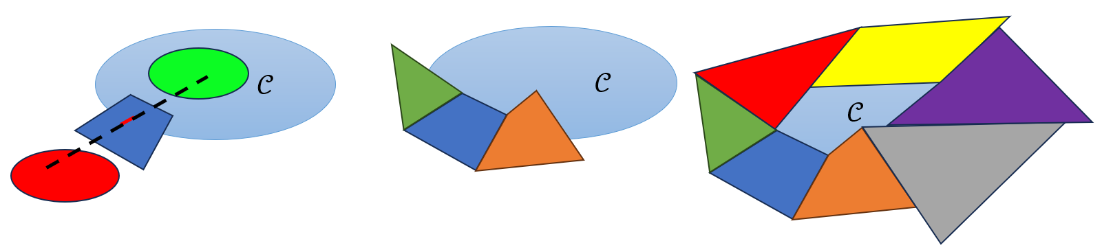
Refer to caption
Figure 2: Illustration of enumerating valid linear regions: We begin by randomly selecting two points—one from the initial set (colored in green) and one from the unsafe set (colored in red)—and iteratively shrinking the segment connecting them until an initial valid linear region is found. The boundary propagation algorithm then expands from this region to identify neighboring valid linear regions. By iteratively applying this propagation step, the algorithm eventually enumerates all valid linear regions.

Searching for an Initial Valid Linear Region

We use the following procedure to search for an initial valid linear region.

  • 1.

    Randomly select points until two points 𝒙1,𝒙2\bm{x}_{1},\bm{x}_{2} are found such that h​(𝒙1)​h​(𝒙2)<0h(\bm{x}_{1})h(\bm{x}_{2})<0. For example, 𝒙1\bm{x}_{1} can be sampled from the unsafe set and 𝒙2\bm{x}_{2} from the initial set.

  • 2.

    Utilize the method of the bisection to shrink the length of the line segment {t​𝒙1+(1−t)​𝒙2:0≤t≤1}\{t\bm{x}_{1}+(1-t)\bm{x}_{2}:0\leq t\leq 1\}, until ‖𝒙1−𝒙2‖≤ϵ\|\bm{x}_{1}-\bm{x}_{2}\|\leq\epsilon, where ϵ>0\epsilon>0 is a predefined threshold. Specifically, suppose initially h​(𝒙1)<0,h​(𝒙2)>0h(\bm{x}_{1})<0,h(\bm{x}_{2})>0, if h​(𝒙1+𝒙22)<0h(\frac{\bm{x}_{1}+\bm{x}_{2}}{2})<0, then 𝒙1:=𝒙1+𝒙22\bm{x}_{1}:=\frac{\bm{x}_{1}+\bm{x}_{2}}{2}, else 𝒙2:=𝒙1+𝒙22\bm{x}_{2}:=\frac{\bm{x}_{1}+\bm{x}_{2}}{2}.

  • 3.

    Compute the interval hull IntHull⁡({𝒙1,𝒙2})\operatorname{IntHull}(\{\bm{x}_{1},\bm{x}_{2}\}) of 𝒙1\bm{x}_{1} and 𝒙2\bm{x}_{2}, and use Interval Bound Propagation (IBP) to determine the candidate activation indicator 𝒞′\mathscr{C}^{\prime}. For each neuron jj in layer ii with input interval [l1,l2][l_{1},l_{2}]:

    • –

      if l1>0l_{1}>0, set 𝒔i​(j):=1\bm{s}_{i}(j):=1;

    • –

      if l2<0l_{2}<0, set 𝒔i​(j):=0\bm{s}_{i}(j):=0;

    • –

      else, set 𝒔i​(j):=−1\bm{s}_{i}(j):=-1.

  • 4.

    Generate all feasible activation indicators 𝒞\mathscr{C} from 𝒞′\mathscr{C}^{\prime} by replacing each −1-1 in 𝒔i​(j)\bm{s}_{i}(j) with both 1 and 0.

  • 5.

    For each feasible activation indicator 𝒞\mathscr{C}, check whether 𝒳​(𝒞)\mathcal{X}(\mathscr{C}) passes the Valid Test below. If a valid indicator is found, denote it by 𝒞0\mathscr{C}_{0}, and take the corresponding region 𝒳​(𝒞0)\mathcal{X}(\mathscr{C}_{0}) as the initial valid linear region.

Valid Test

When 𝒳​(𝒞)\mathcal{X}(\mathscr{C}) is an nn-dimensional valid linear region, it follows that dim(∂𝒞∩𝒳​(𝒞))=n−1\dim(\partial\mathcal{C}\cap\mathcal{X}(\mathscr{C}))=n-1. Therefore, the validity of 𝒳​(𝒞)\mathcal{X}(\mathscr{C}) can be verified by checking whether this dimensional condition holds. Note that the redundant case where ∂𝒞∩𝒳​(𝒞)=𝒳​(𝒞)\partial\mathcal{C}\cap\mathcal{X}(\mathscr{C})=\mathcal{X}(\mathscr{C}) can also be included, but this does not affect the correctness of our method.

Given an activated region of the form 𝒳​(𝒞)={𝒙∈ℝn:𝑨​𝒙≤𝒅}\mathcal{X}(\mathscr{C})=\{\bm{x}\in\mathbb{R}^{n}:\bm{A}\bm{x}\leq\bm{d}\}, define the set 𝒫=∂𝒞∩𝒳​(𝒞)\mathcal{P}=\partial\mathcal{C}\cap\mathcal{X}(\mathscr{C}) and let 𝑨~=[𝑨;𝒘⊤​(𝒞);−𝒘⊤​(𝒞)],𝒅~=[𝒅;−𝒃​(𝒞);𝒃​(𝒞)]\tilde{\bm{A}}=[\bm{A};\bm{w}^{\top}(\mathscr{C});-\bm{w}^{\top}(\mathscr{C})],\tilde{\bm{d}}=[\bm{d};-\bm{b}(\mathscr{C});\bm{b}(\mathscr{C})], then 𝒫={𝒙∈ℝn:𝑨~​𝒙≤𝒅~}\mathcal{P}=\{\bm{x}\in\mathbb{R}^{n}:\tilde{\bm{A}}\bm{x}\leq\tilde{\bm{d}}\} is also a polyhedron. In a system of linear inequalities 𝑨​𝒙≤𝒅\bm{A}\bm{x}\leq\bm{d}, the inequality 𝑨​(j)​𝒙≤𝒅​(j),j∈{1,⋯,rows(𝑨)}\bm{A}(j)\bm{x}\leq\bm{d}(j),j\in\{1,\cdots,\operatorname*{rows}(\bm{A})\}, is called an implicit equality if 𝑨​(j)​𝒙=𝒅​(j)\bm{A}(j)\bm{x}=\bm{d}(j) holds for all solutions of the system 𝑨​𝒙≤𝒅\bm{A}\bm{x}\leq\bm{d}. We denote by 𝑨=​𝒙≤𝒅=\bm{A}^{=}\bm{x}\leq\bm{d}^{=} the system consisting of all implicit equalities within 𝑨​𝒙≤𝒅\bm{A}\bm{x}\leq\bm{d}.

To identify the implicit equalities in 𝒫={𝒙∈ℝn:𝑨~​𝒙≤𝒅~}\mathcal{P}=\{\bm{x}\in\mathbb{R}^{n}:\tilde{\bm{A}}\bm{x}\leq\tilde{\bm{d}}\}, we solve the following pair of LPs for each row j=1,⋯,rows(𝑨~)j=1,\cdots,\operatorname*{rows}(\tilde{\bm{A}}):

min𝒙⁡𝑨~​(j)​𝒙\displaystyle\min_{\bm{x}}\tilde{\bm{A}}(j)\bm{x} max𝒙⁡𝑨~​(j)​𝒙\displaystyle\max_{\bm{x}}\tilde{\bm{A}}(j)\bm{x}
s.t.​𝑨~​𝒙≤𝒅~\displaystyle\text{s.t.}~\tilde{\bm{A}}\bm{x}\leq\tilde{\bm{d}} s.t.​𝑨~​𝒙≤𝒅~\displaystyle\text{s.t.}~\tilde{\bm{A}}\bm{x}\leq\tilde{\bm{d}}

If the optimal values of both LPs are equal, then 𝑨~​(j)​𝒙≤𝒅~​(j)\tilde{\bm{A}}(j)\bm{x}\leq\tilde{\bm{d}}(j) is an implicit equality. According to (Conforti et al. 2014, Theorem 4.17), the dimension of 𝒫\mathcal{P} satisfies dim(𝒫)=n−rank(𝑨~=)\dim(\mathcal{P})=n-\operatorname*{rank}(\tilde{\bm{A}}^{=}). Therefore, if rank(𝑨~=)=1\operatorname*{rank}(\tilde{\bm{A}}^{=})=1, then dim(𝒫)=n−1\dim(\mathcal{P})=n-1.

Boundary Propagation Algorithm

Next we introduce the boundary propagation algorithm, which can enumerate all valid activation indicators, i.e., the set 𝒜≜{𝒞:𝒳​(𝒞)​ is a valid linear region}\mathcal{A}\triangleq\{\mathscr{C}:\mathcal{X}(\mathscr{C})\text{ is a valid linear region}\}. This algorithm proceeds as follows:

  1. 1.

    Initialize the set of valid activation indicators as 𝒜:={𝒞0}\mathcal{A}:=\{\mathscr{C}_{0}\} and the visited set as ℬ:=∅\mathcal{B}:=\emptyset.

  2. 2.

    Select an activation indicator 𝒞\mathscr{C} in 𝒜∖ℬ\mathcal{A}\setminus\mathcal{B} and add 𝒞\mathscr{C} to ℬ\mathcal{B}. Apply the method from (Maréchal and Périn 2017) to remove the redundant constraints in 𝒳​(𝒞)={𝒙∈ℝn:𝑨​𝒙≤𝒅}\mathcal{X}(\mathscr{C})=\{\bm{x}\in\mathbb{R}^{n}:\bm{A}\bm{x}\leq\bm{d}\}. For each j=1,⋯,rows(𝑨)j=1,\cdots,\operatorname*{rows}(\bm{A}), solve the following LP feasibility problem to find the facet of 𝒳​(𝒞)\mathcal{X}(\mathscr{C}) which has the intersection with ∂𝒞\partial\mathcal{C}.

    {𝒘​(𝒞)⊤​𝒙+b​(𝒞)=0𝑨​(j)​𝒙=𝒅​(j)𝑨​(k)​𝒙≤𝒅​(k),k∈{1,⋯,rows(𝑨)}∖{j}\begin{cases}\bm{w}(\mathscr{C})^{\top}\bm{x}+b(\mathscr{C})=0\\ \bm{A}(j)\bm{x}=\bm{d}(j)\\ \bm{A}(k)\bm{x}\leq\bm{d}(k),k\in\{1,\cdots,\operatorname*{rows}(\bm{A})\}\setminus\{j\}\end{cases}

    If the above LP feasibility problem admits a feasible solution 𝒙⋆\bm{x}^{\star}, then enumerate all feasible activation indicators that are activated by 𝒙⋆\bm{x}^{\star}. For each indicator that passes the Valid Test, add it to the set 𝒜\mathcal{A}.

  3. 3.

    The algorithm terminates when 𝒜=ℬ\mathcal{A}=\mathcal{B}, meaning all valid activation indicators have been explored and no new ones have been found.

Remark 3.

When the system dimension is 2, the number of facets of 𝒳​(𝒞)\mathcal{X}(\mathscr{C}) that intersect ∂𝒞\partial\mathcal{C} is at most 4. Therefore once four such facets have been identified, it is unnecessary to examine the remaining facets.

For ReLU neural networks, the partitioning of the input space exhibits a special structure: every nn-dimensional linear region shares a facet with each of its adjacent linear regions. This property arises from the fact that the partitioning is generated through a sequence of hyperplanes, layer by layer (Raghu et al. 2017; Serra et al. 2018). Moreover, since ∂𝒞\partial\mathcal{C} is contained within the union of valid linear regions (see Proposition 1), if we further assume that ∂𝒞\partial\mathcal{C} is connected, then given an initial valid linear region, one can examine its facets to identify those intersecting the boundary. By recursively expanding to adjacent regions via these shared facets, we can enumerate all valid linear regions. The following theorem formalizes this claim.

Theorem 4.

Assuming that ∂𝒞\partial\mathcal{C} is connected, then the boundary propagation algorithm can identify all valid linear regions.

Verification and Falsification in Each Valid Linear Region

After enumerating all valid linear regions, we can verify or falsify the three conditions in Definition 2 — positively invariant, initial set and unsafe set conditions — within each valid linear region.

the Positively Invariant Condition

The necessary and sufficient condition in Theorem 3 can be described as a quantified formula:

∀𝒞∈𝒜,∀𝒙\displaystyle\forall\mathscr{C}\in\mathcal{A},\forall\bm{x} (𝒙∈∂𝒞∩𝒳​(𝒞)→𝒘​(𝒞)⊤​𝒇​(𝒙)≥0).\displaystyle\left(\bm{x}\in\partial\mathcal{C}\cap\mathcal{X}(\mathscr{C})\rightarrow\bm{w}(\mathscr{C})^{\top}\bm{f}(\bm{x})\geq 0\right). (10)

We can translate (10) into an SMT problem that determines whether the following quantifier-free formula with Disjunctive Normal Form (DNF) is satisfiable (SAT) or not (UNSAT).

⋁𝒞∈𝒜\displaystyle\bigvee_{\mathscr{C}\in\mathcal{A}} (𝒘(𝒞)⊤𝒙+b(𝒞)=0∧𝒙∈𝒳(𝒞)\displaystyle\left(\bm{w}(\mathscr{C})^{\top}\bm{x}+b(\mathscr{C})=0\wedge\bm{x}\in\mathcal{X}(\mathscr{C})\right. (11)
∧𝒘(𝒞)⊤𝒇(𝒙)<0).\displaystyle\left.\wedge\bm{w}(\mathscr{C})^{\top}\bm{f}(\bm{x})<0\right).

If the SMT problem (11) is proven to be UNSAT, then the Boolean value of (10) is true, implying that 𝒞\mathcal{C} is positively invariant under system (2). When the system (2) is polynomial, the SMT (11) can be solved using an SMT solver that employs Cylindrical Algebraic Decomposition (Caviness and Johnson 2012), such as Z3 (De Moura and Bjørner 2008). In this case, verification by solving (11) is both sound and complete: an UNSAT return implies positive invariance of 𝒞\mathcal{C}, while a SAT return indicates the falsification of positive invariance. When the system (2) is non-polynomial, we can use dReal (Gao et al. 2013), an SMT solver that supports non-polynomial functions such as trigonometric and exponential functions. dReal employs δ\delta-complete decision procedures, returning either UNSAT or δ\delta-SAT, where δ\delta is a user-specified numerical error bound. Therefore, positive invariance verification using dReal is sound: when dReal returns UNSAT for SMT (11), 𝒞\mathcal{C} is positively invariant. However, a “δ\delta-SAT” result does not necessarily falsify positive invariance due to potential numerical errors.

The quantified formula (10) can also be described as a series of optimization problems: for each valid linear region 𝒳​(𝒞),𝒞∈𝒜\mathcal{X}(\mathscr{C}),\mathscr{C}\in\mathcal{A}, we solve the following optimization.

min𝒙⁡𝒘​(𝒞)⊤​𝒇​(𝒙)s.t.{𝒘​(𝒞)⊤​𝒙+b​(𝒞)=0,𝒙∈𝒳​(𝒞).\begin{split}&\min_{\bm{x}}\bm{w}(\mathscr{C})^{\top}\bm{f}(\bm{x})\\ \text{s.t.}~&\begin{cases}\bm{w}(\mathscr{C})^{\top}\bm{x}+b(\mathscr{C})=0,\\ \bm{x}\in\mathcal{X}(\mathscr{C}).\end{cases}\end{split} (12)

If the optimal value of (12) is non-negative, the positive invariance condition is satisfied for 𝒞\mathscr{C}. When all activation indicators in 𝒜\mathcal{A} pass the verification, we can deduce that 𝒞\mathcal{C} is positively invariant for system (2); otherwise, it is not. When the system (2) is linear, the optimization is an LP, therefore if the optimal value of (12) exists, it can be obtained by the simplex method or interior-point method. However, when the the system (2) is nonlinear, the optimization (12) may be nonconvex, making it challenging to obtain the optimal value. Whereas, we we can utilize (12) to falsify the positive invariance, Specifically, if there exists a valid linear region 𝒳​(𝒞),𝒞∈𝒜\mathcal{X}(\mathscr{C}),\mathscr{C}\in\mathcal{A} such that (12) yields a negative feasible value, then 𝒞\mathcal{C} is not positively invariant.

Remark 4.

The condition based on the Bouligand tangent cone cannot be directly translated into a series of optimization problems, in contrast to condition derived from the Clarke tangent cone. This limitation arises from the presence of strict inequalities — specifically, the restriction “for 𝐱∈Int⁡𝒳i\bm{x}\in\operatorname{Int}{\mathcal{X}_{i}} (𝐀i𝐱<𝐝i)\bm{A}_{i}\bm{x}<\bm{d}_{i})” in first assertion of Proposition 1 — which are not permitted in standard optimization formulations. The detailed explanation can be found in the appendix.

the Initial and Unsafe Set Conditions

We can also encode the verification of the initial and unsafe set conditions as SMT and optimization problems like the positively invariant condition. To this end, we introduce the following propositions, which provide necessary and sufficient conditions for these conditions.

Proposition 3.

𝒮I⊂𝒞\mathcal{S}_{I}\subset\mathcal{C} if and only if 𝒮I∩∂𝒞=∅\mathcal{S}_{I}\cap\partial\mathcal{C}=\emptyset and 𝒮I∩Int⁡𝒞≠∅\mathcal{S}_{I}\cap\operatorname{Int}\mathcal{C}\neq\emptyset.

Proposition 4.

𝒮U∩𝒞=∅\mathcal{S}_{U}\cap\mathcal{C}=\emptyset if and only if 𝒮U∩∂𝒞=∅\mathcal{S}_{U}\cap\partial\mathcal{C}=\emptyset and 𝒮U∩𝒞c≠∅\mathcal{S}_{U}\cap\mathcal{C}^{c}\neq\emptyset.

The condition 𝒮I∩∂𝒞=∅\mathcal{S}_{I}\cap\partial\mathcal{C}=\emptyset can also be described as a quantified formula:

∀𝒞∈𝒜,∀𝒙​(𝒙∈∂𝒞∩𝒳​(𝒞)→hI​(𝒙)≤0).\displaystyle\forall\mathscr{C}\in\mathcal{A},\forall\bm{x}\,\left(\bm{x}\in\partial\mathcal{C}\cap\mathcal{X}(\mathscr{C})\rightarrow h_{I}(\bm{x})\leq 0\right). (13)

Similar to the positive invariance condition, the quantified formula (13) can be encoded into SMT and optimization problems. For simplicity, we present the details in the appendix.

To verify 𝒮I∩Int⁡𝒞≠∅\mathcal{S}_{I}\cap\operatorname{Int}\mathcal{C}\neq\emptyset, we can randomly select a point 𝒙∈𝒮I\bm{x}\in\mathcal{S}_{I} and check whether hI​(𝒙)>0h_{I}(\bm{x})>0. If both conditions are satisfied, we conclude that 𝒮I⊂𝒞\mathcal{S}_{I}\subset\mathcal{C}. Otherwise, the verification fails.

Note that the condition in Proposition 4 for verifying the unsafe set condition 𝒮U∩𝒞=∅\mathcal{S}_{U}\cap\mathcal{C}=\emptyset is analogous to that used for verifying the initial set condition. Therefore, a similar verification procedure can be applied to the unsafe set condition as well.

Experiments

In this section, we evaluate the proposed method to demonstrate the validity and effectiveness of our verification algorithm. Specifically, we conduct experiments on four systems: Arch3, Complex, Linear4d, and Decay. Among them, Linear4d is a linear system, while the others are nonlinear. System descriptions, experimental settings, and detailed experimental results are provided in the appendix.

For linear systems, we only solve the optimization problem (12) to check the positive invariance condition, as it reduces to an LP whose optimal value can be reliably obtained when it exists. For nonlinear systems, we first solve the optimization (12). If there exists a valid linear region for which the suboptimal value is negative, then the positive invariance condition is falsified. Otherwise, if all instances of (12) yield nonnegative suboptimal values for each 𝒞∈𝒜\mathscr{C}\in\mathcal{A}, we proceed to solve the SMT problem (11) using the dReal solver (Gao et al. 2013). If dReal returns UNSAT for every region, positive invariance is verified. However, if it returns δ\delta-SAT for any region, the validity of the certificate remains inconclusive. The same procedure is applied to verify the initial set and unsafe set conditions.

We compare our method with that in (Zhang et al. 2023), as it is, to the best of our knowledge, the only method that does not rely on the Heaviside step function assumption for the derivative of the ReLU activation. Notably, our method supports both verification and falsification of barrier certificates, whereas the method in (Zhang et al. 2023) only performs verification. Consequently, if a certificate fails their test, no conclusion can be drawn about its correctness. Furthermore, the correctness guarantees in (Zhang et al. 2023) hold only if all the involved optimization problems return optimal solutions. In practice, however, solvers often yield suboptimal results in nonlinear programming, potentially undermining the reliability of their verification.

Refer to caption
(a) (a)
Refer to caption
(b) (b)
Figure 3: Enumerated valid linear regions and the vector fields of system Arch3.

The running time and validity of barrier certificates for each case are summarized in Table 1. Our method successfully verifies or falsifies all cases, whereas the approach in (Zhang et al. 2023) can only verify five out of seven barrier certificates in the two-dimensional system Arch3. In other cases, it either returns “unknown” or crashes due to memory exhaustion. Furthermore, their results are reliable only when all optimal values of the underlying optimizations can be obtained, which is difficult to rigorously verify in nonlinear programming. In terms of running time, our method consistently outperforms theirs, particularly in high-dimensional systems. This improvement stems from the fact that our algorithm enumerates far fewer regions than (Zhang et al. 2023), as discussed in Remark 2. Figure 3 illustrates the valid linear regions enumerated by our boundary propagation algorithm for the first barrier certificate in system Arch3.

Table 1: The first two columns list the system names and the neural network architectures of the barrier certificates, where HNN denotes the number of neurons in each hidden layer. We denote the total running time and barrier certificate validity in our method as to​u​rt_{our} and Vo​u​r\text{V}_{our}, respectively, and use tZt_{Z} and VZ\text{V}_{Z} for the corresponding results from (Zhang et al. 2023). A dash (−-) indicates that the program crashed due to memory exhaustion. A ✓ indicates that the barrier certificate is verified (✓\checkmark means verified under the assumption that all optimal values of the underlying optimizations can be obtained), while ✗ indicates falsification. A ? denotes that the validity of the barrier certificate is unknown.
Case HNN to​u​rt_{our} tZt_{Z} Vo​u​r\text{V}_{our} VZ\text{V}_{Z}
Arch3 (2-d) (nonlinear) 32 3.89 24.10 ✓ ✓\checkmark
64 28.40 141.01 ✓ ✓\checkmark
96 94.75 528.36 ✓ ✓\checkmark
128 204.78 198.17 ✗ ?
32-32 19.75 41.10 ✓ ✓\checkmark
64-64 215.99 283.00 ✓ ✓\checkmark
96-96 774.27 1644.60 ✗ ?
Complex (3-d) (nonlinear) 32 5.29 135.22 ✓ ?
64 92.36 698.35 ✓ ?
96 469.53 1377.00 ✓ ?
32-32 79.57 1132.23 ✓ ?
64-64 500.08 −- ✗ −-
96-96 19686.48 −- ✓ −-
Linear4d (4-d) (linear) 16 9.61 286.46 ✓ ?
32 88.12 1110.54 ✓ ?
48 9992.90 −- ✓ −-
8-8 7.84 212.19 ✓ ?
12-12 55.05 593.78 ✓ ?
16-16 524.73 2243.71 ✗ ?
24-24 22571.44 −- ✗ −-
Decay (6-d) (nonlinear) 20 19842.22 −- ✓ −-
8-8 347.72 4381.28 ✓ ?
10-10 1953.08 4035.94 ✗ ?
12-12 31112.56 −- ✗ −-

Conclusion

In this paper, we proposed a necessary and sufficient condition for verifying ReLU neural barrier certificates and developed a corresponding algorithm that supports both verification and falsification. To the best of our knowledge, this is the first method capable of falsifying ReLU neural barrier certificates, thereby filling a critical gap for their reliable application in safety-critical systems. Through numerical experiments, we demonstrated that our method achieves superior verification performance compared to existing approaches, particularly in high-dimensional systems.

References

  • A. Abate, D. Ahmed, A. Edwards, M. Giacobbe, and A. Peruffo (2021) FOSSIL: a software tool for the formal synthesis of lyapunov functions and barrier certificates using neural networks. In Proceedings of the 24th international conference on hybrid systems: computation and control, pp. 1–11. Cited by: Introduction.
  • A. D. Ames, S. Coogan, M. Egerstedt, G. Notomista, K. Sreenath, and P. Tabuada (2019) Control barrier functions: theory and applications. In 2019 18th European control conference (ECC), pp. 3420–3431. Cited by: Introduction, Introduction, Tangent Cones and Invariance Conditions.
  • A. D. Ames, X. Xu, J. W. Grizzle, and P. Tabuada (2016) Control barrier function based quadratic programs for safety critical systems. IEEE Transactions on Automatic Control 62 (8), pp. 3861–3876. Cited by: Tangent Cones and Invariance Conditions.
  • J. Aubin and H. Frankowska (2009) Set-valued analysis. Springer Science & Business Media. Cited by: Other Definitions of Tangent Cones, Proof., Proof., Proof., Definition 4.
  • B. F. Caviness and J. R. Johnson (2012) Quantifier elimination and cylindrical algebraic decomposition. Springer Science & Business Media. Cited by: the Positively Invariant Condition.
  • A. Clark (2021) Verification and synthesis of control barrier functions. In 2021 60th IEEE Conference on Decision and Control (CDC), pp. 6105–6112. Cited by: Introduction.
  • F. H. Clarke, Y. S. Ledyaev, R. J. Stern, and P. R. Wolenski (2008) Nonsmooth analysis and control theory. Vol. 178, Springer Science & Business Media. Cited by: Tangent Cones and Invariance Conditions, Definition 4, Lemma 4, Theorem 1.
  • F. H. Clarke (1990) Optimization and nonsmooth analysis. edition, Society for Industrial and Applied Mathematics, . External Links: Document, Link, https://epubs.siam.org/doi/pdf/10.1137/1.9781611971309 Cited by: Lemma 2.
  • M. Conforti, G. Cornuéjols, and G. Zambelli (2014) Integer programming. Graduate Texts in Mathematics, Springer International Publishing. External Links: ISBN 9783319110080, LCCN 2014952029, Link Cited by: Valid Test.
  • L. Dai, T. Gan, B. Xia, and N. Zhan (2017) Barrier certificates revisited. Journal of Symbolic Computation 80, pp. 62–86. Cited by: Introduction.
  • C. Dawson, S. Gao, and C. Fan (2023) Safe control with learned certificates: a survey of neural lyapunov, barrier, and contraction methods for robotics and control. IEEE Transactions on Robotics 39 (3), pp. 1749–1767. Cited by: Introduction, Introduction.
  • C. Dawson, Z. Qin, S. Gao, and C. Fan (2022) Safe nonlinear control using robust neural lyapunov-barrier functions. In Conference on Robot Learning, pp. 1724–1735. Cited by: Introduction.
  • L. De Moura and N. Bjørner (2008) Z3: an efficient smt solver. In International conference on Tools and Algorithms for the Construction and Analysis of Systems, pp. 337–340. Cited by: the Positively Invariant Condition.
  • S. Gao, S. Kong, and E. M. Clarke (2013) DReal: an smt solver for nonlinear theories over the reals. In International conference on automated deduction, pp. 208–214. Cited by: the Positively Invariant Condition, Experiments.
  • K. He, X. Zhang, S. Ren, and J. Sun (2015) Delving deep into rectifiers: surpassing human-level performance on imagenet classification. In Proceedings of the IEEE international conference on computer vision, pp. 1026–1034. Cited by: Introduction.
  • H. Hu, Y. Yang, T. Wei, and C. Liu (2024) Verification of neural control barrier functions with symbolic derivative bounds propagation. In 8th Annual Conference on Robot Learning, Cited by: 1st item, Introduction.
  • S. G. Johnson (2007) The NLopt nonlinear-optimization package. Note: https://github.com/stevengj/nlopt Cited by: Experimental Settings.
  • S. Liu, C. Liu, and J. Dolan (2023) Safe control under input limits with neural control barrier functions. In Conference on Robot Learning, pp. 1970–1980. Cited by: Introduction.
  • A. L. Maas, A. Y. Hannun, A. Y. Ng, et al. (2013) Rectifier nonlinearities improve neural network acoustic models. In Proc. icml, Vol. 30, pp. 3. Cited by: Introduction.
  • A. Maréchal and M. Périn (2017) Efficient elimination of redundancies in polyhedra using raytracing. In Verification, Model Checking, and Abstract Interpretation (VMCAI), Vol. 10145. Cited by: item 2.
  • F. B. Mathiesen, S. C. Calvert, and L. Laurenti (2022) Safety certification for stochastic systems via neural barrier functions. IEEE Control Systems Letters 7, pp. 973–978. Cited by: Introduction.
  • G. F. Montufar, R. Pascanu, K. Cho, and Y. Bengio (2014) On the number of linear regions of deep neural networks. Advances in neural information processing systems 27. Cited by: ReLU Neural Network.
  • Z. Qin, K. Zhang, Y. Chen, J. Chen, and C. Fan (2021) Learning safe multi-agent control with decentralized neural barrier certificates. arXiv preprint arXiv:2101.05436. Cited by: Introduction.
  • M. Raghu, B. Poole, J. Kleinberg, S. Ganguli, and J. Sohl-Dickstein (2017) On the expressive power of deep neural networks. In international conference on machine learning, pp. 2847–2854. Cited by: Boundary Propagation Algorithm.
  • T. Serra, C. Tjandraatmadja, and S. Ramalingam (2018) Bounding and counting linear regions of deep neural networks. In International conference on machine learning, pp. 4558–4566. Cited by: Boundary Propagation Algorithm.
  • R. Tedrake and the Drake Development Team (2019) Drake: model-based design and verification for robotics. External Links: Link Cited by: Experimental Settings.
  • W. Xiao, T. Wang, R. Hasani, M. Chahine, A. Amini, X. Li, and D. Rus (2023) Barriernet: differentiable control barrier functions for learning of safe robot control. IEEE Transactions on Robotics 39 (3), pp. 2289–2307. Cited by: Introduction.
  • H. Zhang, Z. Qin, S. Gao, and A. Clark (2024) SEEV: synthesis with efficient exact verification for relu neural barrier functions. arXiv preprint arXiv:2410.20326. Cited by: Introduction.
  • H. Zhang, J. Wu, Y. Vorobeychik, and A. Clark (2023) Exact verification of relu neural control barrier functions. Advances in neural information processing systems 36, pp. 5685–5705. Cited by: 1st item, Introduction, Introduction, Table 1, Experiments, Experiments, Experimental Settings, Detailed Explanation for Remark 4, Lemma 1, Remark 2.
  • H. Zhao, X. Zeng, T. Chen, Z. Liu, and J. Woodcock (2021a) Learning safe neural network controllers with barrier certificates. Formal Aspects of Computing 33, pp. 437–455. Cited by: Introduction.
  • H. Zhao, X. Zeng, T. Chen, and Z. Liu (2020) Synthesizing barrier certificates using neural networks. In Proceedings of the 23rd international conference on hybrid systems: Computation and control, pp. 1–11. Cited by: Introduction, Experimental Settings.
  • Q. Zhao, X. Chen, Y. Zhang, M. Sha, Z. Yang, W. Lin, E. Tang, Q. Chen, and X. Li (2021b) Synthesizing relu neural networks with two hidden layers as barrier certificates for hybrid systems. In Proceedings of the 24th International Conference on Hybrid Systems: Computation and Control, pp. 1–11. Cited by: Introduction.
  • Q. Zhao, X. Chen, Z. Zhao, Y. Zhang, E. Tang, and X. Li (2022) Verifying neural network controlled systems using neural networks. In Proceedings of the 25th ACM International Conference on Hybrid Systems: Computation and Control, pp. 1–11. Cited by: 1st item, Introduction, Explanation for the Lack of Mathematical Rigor in the Derivative Assumption.
  • G. M. Ziegler (2012) Lectures on polytopes. Vol. 152, Springer Science & Business Media. Cited by: Definition 7.

Appendix

Explanation for the Lack of Mathematical Rigor in the Derivative Assumption

In this section, we explain why assuming that the derivative of the ReLU function is the Heaviside function is mathematically non-rigorous for verifying positive invariance. To this end, we first characterize the tangent cones of the 0-superlevel set of a continuously differentiable function in the following lemma.

Lemma 2 ((Clarke 1990, Theorem 2.4.7)).

Let 𝒮={𝐳∈ℝn:h​(𝐳)≥0}\mathcal{S}=\{\bm{z}\in\mathbb{R}^{n}:h(\bm{z})\geq 0\}, where h:ℝn→ℝh:\mathbb{R}^{n}\rightarrow\mathbb{R} is continuously differentiable, and let 𝐱\bm{x} be a point satisfying h​(𝐱)=0h(\bm{x})=0. Suppose that ∇h​(𝐱)≠𝟎\nabla h(\bm{x})\neq\bm{0}, then 𝒮\mathcal{S} is regular at 𝐱\bm{x} and

T𝒮B​(𝒙)=T𝒮C​(𝒙)={𝒗∈ℝn:∇h​(𝒙)​𝒗≥0}.T_{\mathcal{S}}^{B}(\bm{x})=T_{\mathcal{S}}^{C}(\bm{x})=\{\bm{v}\in\mathbb{R}^{n}:\nabla h(\bm{x})\bm{v}\geq 0\}.

Combining this lemma with Theorem 1, we obtain the following proposition.

Proposition 5.

Let 𝒮={𝐳∈ℝn:h​(𝐳)≥0}\mathcal{S}=\{\bm{z}\in\mathbb{R}^{n}:h(\bm{z})\geq 0\}, where h:ℝn→ℝh:\mathbb{R}^{n}\rightarrow\mathbb{R} is continuously differentiable. Suppose that for all 𝐱∈𝒮\bm{x}\in\mathcal{S} with h​(𝐱)=0h(\bm{x})=0, we have ∇h​(𝐱)≠𝟎\nabla h(\bm{x})\neq\bm{0}. Then 𝒮\mathcal{S} is positively invariant under the system (2) if and only if

∇h​(𝒙)​𝒇​(𝒙)≥0,∀𝒙∈{𝒙∈ℝn:h​(𝒙)=0}.\nabla h(\bm{x})\bm{f}(\bm{x})\geq 0,\forall\bm{x}\in\{\bm{x}\in\mathbb{R}^{n}:h(\bm{x})=0\}.

Some existing work (e.g., (Zhao et al. 2022)) applies Proposition 5 to verify the positive invariance of the 0-superlevel set of a ReLU neural barrier certificate. However, this is inconsistent with the requirement that hh is continuously differentiable, since a ReLU neural barrier certificate is inherently non-differentiable at certain points. Even if the derivative of ReLU function is forcibly defined as the Heaviside function, the latter’s discontinuity still violates the requirement of continuous differentiability. Therefore, Proposition 5 is not applicable to the verification of ReLU neural barrier certificates.

Background of Polyhedron

Definition 6 (Affine hull).

Given a set of points 𝒮={𝐱1,𝐱2,…,𝐱k}⊂ℝn\mathcal{S}=\{\bm{x}_{1},\bm{x}_{2},\ldots,\bm{x}_{k}\}\subset\mathbb{R}^{n}, the affine hull of 𝒮\mathcal{S} is defined as

aff⁡(𝒮)={∑i=1kλi​𝒙i|∑i=1kλi=1,λi∈ℝ}.\operatorname{aff}(\mathcal{S})=\left\{\sum_{i=1}^{k}\lambda_{i}\bm{x}_{i}\,\middle|\,\sum_{i=1}^{k}\lambda_{i}=1,\ \lambda_{i}\in\mathbb{R}\right\}.

The dimension of an affine hull is the dimension of the corresponding linear vector space.

Definition 7 (Polyhedron, (Ziegler 2012)).

Polyhedron is an intersection of closed halfspaces: a set 𝒫⊆ℝd\mathcal{P}\subseteq\mathbb{R}^{d} presented in the form 𝒫={𝐱∈ℝd:𝐀​𝐱≤𝐝} for some ​𝐀∈ℝm×d,𝐝∈ℝm\mathcal{P}=\left\{\bm{x}\in\mathbb{R}^{d}:\bm{A}\bm{x}\leq\bm{d}\right\}\quad\text{ for some }\bm{A}\in\mathbb{R}^{m\times d},\bm{d}\in\mathbb{R}^{m}. The dimension of a polyhedron is the dimension of its affine hull: dim⁡(𝒫)≜dim⁡(aff⁡(𝒫))\operatorname{dim}(\mathcal{P})\triangleq\operatorname{dim}(\operatorname{aff}(\mathcal{P})).

Definition 8 (Face).

Let 𝒫⊆ℝd\mathcal{P}\subseteq\mathbb{R}^{d} be a convex polyhedron. A linear inequality 𝐜⊤​𝐱≤c0\bm{c}^{\top}\bm{x}\leq c_{0} is valid for 𝒫\mathcal{P} if it is satisfied for all points 𝐱∈𝒫\bm{x}\in\mathcal{P}. A face of 𝒫\mathcal{P} is any set of the form

ℱ=𝒫∩{𝒙∈ℝd:𝒄⊤​𝒙=c0},\mathcal{F}=\mathcal{P}\cap\left\{\bm{x}\in\mathbb{R}^{d}:\bm{c}^{\top}\bm{x}=c_{0}\right\},

where 𝐜⊤​𝐱≤c0\bm{c}^{\top}\bm{x}\leq c_{0} is a valid inequality for 𝒫\mathcal{P}. The dimension of a face is the dimension of its affine hull: dim⁡(ℱ)≜dim⁡(aff⁡(ℱ))\operatorname{dim}(\mathcal{F})\triangleq\operatorname{dim}(\operatorname{aff}(\mathcal{F})).

Faces of a polyhedron 𝒫\mathcal{P} with dimensions 0, 1, dim(𝒫)−2\dim(\mathcal{P})-2, and dim(𝒫)−1\dim(\mathcal{P})-1 are called vertices, edges, ridges, and facets, respectively. The relative interior of 𝒫\mathcal{P}, denoted relind(𝒫)\operatorname*{relind}(\mathcal{P}), is defined as as the interior of 𝒫\mathcal{P} with respect to the embedding of 𝒫\mathcal{P} into its affine hull aff(𝒫)\operatorname*{aff}(\mathcal{P}), in which 𝒫\mathcal{P} is full-dimensional.

Other Definitions of Tangent Cones

The tangent cones in Definition 4 can also be defined in the sense of set-valued analysis:

T𝒮B​(𝒙)≜lim supt→0+𝒮−𝒙t,T_{\mathcal{S}}^{B}(\bm{x})\triangleq\limsup_{t\rightarrow 0^{+}}\frac{\mathcal{S}-\bm{x}}{t}, (14)
T𝒮C​(𝒙)≜lim inft→0+,𝒙′→𝒮𝒙𝒮−𝒙t,T_{\mathcal{S}}^{C}(\bm{x})\triangleq\liminf_{t\rightarrow 0^{+},\bm{x}^{\prime}\stackrel{{\scriptstyle\mathcal{S}}}{{\rightarrow}}\bm{x}}\frac{\mathcal{S}-\bm{x}}{t}, (15)

where 𝒮−𝒙t≜{𝒛−𝒙t,𝒛∈𝒮}\frac{\mathcal{S}-\bm{x}}{t}\triangleq\{\frac{\bm{z}-\bm{x}}{t},\bm{z}\in\mathcal{S}\}, and for details on limits of sets and set-valued maps, we refer the reader to (Aubin and Frankowska 2009).

Equivalently, the tangent cones can be characterized in terms of sequences:

  • •

    𝒗∈T𝒮B​(𝒙)\bm{v}\in T_{\mathcal{S}}^{B}(\bm{x}) if and only if ∃tn→0+\exists t_{n}\rightarrow 0^{+} and ∃𝒗n→𝒗\exists\bm{v}_{n}\rightarrow\bm{v} such that ∀n∈ℕ+,𝒙+tn​𝒗n∈𝒮\forall n\in\mathbb{N}^{+},\bm{x}+t_{n}\bm{v}_{n}\in\mathcal{S}.

  • •

    𝒗∈T𝒮C​(𝒙)\bm{v}\in T_{\mathcal{S}}^{C}(\bm{x}) if and only if ∀tn→0+\forall t_{n}\rightarrow 0^{+}, ∀𝒙n→𝒮𝒙\forall\bm{x}_{n}\stackrel{{\scriptstyle\mathcal{S}}}{{\rightarrow}}\bm{x}, ∃𝒗n→𝒗\exists\bm{v}_{n}\rightarrow\bm{v} such that ∀n∈ℕ+,𝒙n+tn​𝒗n∈𝒮\forall n\in\mathbb{N}^{+},\bm{x}_{n}+t_{n}\bm{v}_{n}\in\mathcal{S}.

Detailed Explanation for Remark 4

In Proposition 1, we state that for any 𝒙∈∂𝒞\bm{x}\in\partial\mathcal{C},

  • 1.

    if 𝒙∈Int⁡𝒳i,i=1,⋯,N\bm{x}\in\operatorname{Int}{\mathcal{X}_{i}},i=1,\cdots,N, then

    T𝒞B​(𝒙)={𝒗∈ℝn:𝒘i⊤​𝒗≥0};\displaystyle T_{\mathcal{C}}^{B}(\bm{x})=\{\bm{v}\in\mathbb{R}^{n}:\bm{w}_{i}^{\top}\bm{v}\geq 0\};
  • 2.

    if 𝒙∈⋂k=1m𝒳ik\bm{x}\in\bigcap_{k=1}^{m}{\mathcal{X}_{i_{k}}} and 𝒙∉ℝn∖⋃k=1m𝒳ik¯,i1,⋯,im∈{1,2,⋯,N}\bm{x}\not\in\overline{\mathbb{R}^{n}\setminus\bigcup_{k=1}^{m}\mathcal{X}_{i_{k}}},i_{1},\cdots,i_{m}\in\{1,2,\cdots,N\}, then

    T𝒞B​(𝒙)=⋃k=1m{𝒗∈ℝn:⋀j∈E𝑨ik​(j)​𝒗≤0∧𝒘ik⊤​𝒗≥0},\displaystyle T_{\mathcal{C}}^{B}(\bm{x})=\bigcup_{k=1}^{m}\{\bm{v}\in\mathbb{R}^{n}:\bigwedge_{j\in E}\bm{A}_{i_{k}}(j)\bm{v}\leq 0\wedge\bm{w}_{i_{k}}^{\top}\bm{v}\geq 0\},

    where the set EE is defined as E≜{j∈{1,⋯,rows(𝑨)}:𝑨ik​(j)​𝒙=𝒅ik​(j)}E\triangleq\{j\in\{1,\cdots,\operatorname*{rows}(\bm{A})\}:\bm{A}_{i_{k}}(j)\bm{x}=\bm{d}_{i_{k}}(j)\}.

Thus, verifying the condition “for all 𝒙∈∂𝒮\bm{x}\in\partial\mathcal{S}, 𝒇​(𝒙)∈T𝒮B​(𝒙)\bm{f}(\bm{x})\in T_{\mathcal{S}}^{B}(\bm{x})” in Theorem 1 can be divided into two parts: (1) verification within the interior of each linear region intersecting the boundary, and (2) verification at their intersections.

To verify the condition “for all 𝒙∈∂𝒮∩Int⁡𝒳i\bm{x}\in\partial\mathcal{S}\cap\operatorname{Int}{\mathcal{X}_{i}}, 𝒇​(𝒙)∈T𝒮B​(𝒙)\bm{f}(\bm{x})\in T_{\mathcal{S}}^{B}(\bm{x})”, the corresponding “optimization formulation” should be

min𝒙⁡𝒘i⊤​𝒇​(𝒙)s.t.{𝒘i⊤​𝒙+b​(𝒞)=0,𝑨i​𝒙<𝒅i.\begin{split}&\min_{\bm{x}}\bm{w}_{i}^{\top}\bm{f}(\bm{x})\\ \text{s.t.}~&\begin{cases}\bm{w}_{i}^{\top}\bm{x}+b(\mathscr{C})=0,\\ \bm{A}_{i}\bm{x}<\bm{d}_{i}.\end{cases}\end{split}

However, the strict inequalities “𝑨i​𝒙<𝒅i\bm{A}_{i}\bm{x}<\bm{d}_{i}” are not permitted in standard optimization formulations (see https://yalmip.github.io/inside/strictinequalities/). To make the optimization problem computationally tractable, these constraints must be relaxed to non-strict ones: 𝑨i​𝒙≤𝒅i\bm{A}_{i}\bm{x}\leq\bm{d}_{i}. This relaxation, however, transforms the condition based on Bouligand tangent cone from necessary and sufficient to merely sufficient. As a result, the optimization method in (Zhang et al. 2023) can only verify, but not falsify, the positive invariance.

Verifying and Falsifying 𝒮I∩∂𝒞=∅\mathcal{S}_{I}\cap\partial\mathcal{C}=\emptyset via SMT and Optimization

We can translate (13) into an SMT problem that determines whether the following quantifier-free formula with Disjunctive Normal Form (DNF) is satisfiable (SAT) or not (UNSAT).

⋁𝒞∈𝒜\displaystyle\bigvee_{\mathscr{C}\in\mathcal{A}} (𝒘​(𝒞)⊤​𝒙+b​(𝒞)=0∧𝒙∈𝒳​(𝒞)∧hI​(𝒙)>0).\displaystyle\left(\bm{w}(\mathscr{C})^{\top}\bm{x}+b(\mathscr{C})=0\wedge\bm{x}\in\mathcal{X}(\mathscr{C})\wedge h_{I}(\bm{x})>0\right). (16)

If the SMT problem (16) is proven to be UNSAT, then the Boolean value of (13) is true, implying that 𝒮I∩∂𝒞=∅\mathcal{S}_{I}\cap\partial\mathcal{C}=\emptyset; In the opposite, when (16) is SAT, then the Boolean value of (13) is false, implying that 𝒮I∩∂𝒞≠∅\mathcal{S}_{I}\cap\partial\mathcal{C}\neq\emptyset.

The quantified formula (13) can also be described as a series of optimization problems: for each valid linear region 𝒳​(𝒞),𝒞∈𝒜\mathcal{X}(\mathscr{C}),\mathscr{C}\in\mathcal{A}, we solve

max𝒙⁡hI​(𝒙)s.t.{𝒘​(𝒞)⊤​𝒙+b​(𝒞)=0,𝒙∈𝒳​(𝒞).\begin{split}&\max_{\bm{x}}h_{I}(\bm{x})\\ \text{s.t.}~&\begin{cases}\bm{w}(\mathscr{C})^{\top}\bm{x}+b(\mathscr{C})=0,\\ \bm{x}\in\mathcal{X}(\mathscr{C}).\end{cases}\end{split} (17)

If all the optimal values of (17) are non-positive for all 𝒞∈𝒜\mathscr{C}\in\mathcal{A}, then 𝒮I∩∂𝒞=∅\mathcal{S}_{I}\cap\partial\mathcal{C}=\emptyset. If there exists a valid linear region 𝒳​(𝒞),𝒞∈𝒜\mathcal{X}(\mathscr{C}),\mathscr{C}\in\mathcal{A} such that (17) yields a positive feasible value, then 𝒮I∩∂𝒞≠∅\mathcal{S}_{I}\cap\partial\mathcal{C}\neq\emptyset.

The verifying and falsifying of the condition 𝒮U∩∂𝒞=∅\mathcal{S}_{U}\cap\partial\mathcal{C}=\emptyset are similar to the ones for 𝒮I∩∂𝒞=∅\mathcal{S}_{I}\cap\partial\mathcal{C}=\emptyset, just simply replacing hIh_{I} with hUh_{U} in (16) and (17).

Auxiliary Lemmas and Proofs

Lemma 3.

Let 𝒮\mathcal{S} be a closed subset of the Banach space XX with norm ∥⋅∥\|\cdot\|, for all ϵ>0\epsilon>0,

T𝒮B​(𝒙)=T𝒮∩B​(𝒙,ϵ)B​(𝒙).\displaystyle T_{\mathcal{S}}^{B}(\bm{x})=T_{\mathcal{S}\cap B(\bm{x},\epsilon)}^{B}(\bm{x}). (18)
Proof.

T𝒮B​(𝒙)⊃T𝒮∩B​(𝒙,ϵ)B​(𝒙)T_{\mathcal{S}}^{B}(\bm{x})\supset T_{\mathcal{S}\cap B(\bm{x},\epsilon)}^{B}(\bm{x}) (if 𝒦⊂ℒ\mathcal{K}\subset\mathcal{L} and 𝒙∈𝒦¯\bm{x}\in\overline{\mathcal{K}}, then T𝒦B​(𝒙)⊂TℒB​(𝒙)T_{\mathcal{K}}^{B}(\bm{x})\subset T_{\mathcal{L}}^{B}(\bm{x}), see (Aubin and Frankowska 2009, Chapter 4)). Next we prove T𝒮B​(𝒙)⊂T𝒮∩B​(𝒙,ϵ)B​(𝒙)T_{\mathcal{S}}^{B}(\bm{x})\subset T_{\mathcal{S}\cap B(\bm{x},\epsilon)}^{B}(\bm{x}).

For 𝒗∈T𝒮B​(𝒙)\bm{v}\in T_{\mathcal{S}}^{B}(\bm{x}), there exists a sequence {tn}\{t_{n}\} satisfying tn→0+t_{n}\rightarrow 0^{+}, then ∃N1>0\exists N_{1}>0 such that ∀n≥N1,tn≤ϵ4​‖𝒗‖\forall n\geq N_{1},t_{n}\leq\frac{\epsilon}{4\|\bm{v}\|}, since 𝒗∈T𝒮B​(𝒙)\bm{v}\in T_{\mathcal{S}}^{B}(\bm{x}), we can find 𝒗n→𝒗\bm{v}_{n}\rightarrow\bm{v} such that ∀n∈ℕ+,𝒙+tn​𝒗n∈𝒮\forall n\in\mathbb{N}^{+},\bm{x}+t_{n}\bm{v}_{n}\in\mathcal{S}. For sequence {𝒗n}\{\bm{v}_{n}\}, ∃N2>0\exists N_{2}>0 such that ∀n≥N2,‖𝒗n−𝒗‖≤‖𝒗‖,‖𝒗n‖≤2​‖𝒗‖\forall n\geq N_{2},\|\bm{v}_{n}-\bm{v}\|\leq\|\bm{v}\|,\|\bm{v}_{n}\|\leq 2\|\bm{v}\|. Let N=max⁡{N1,N2}N=\max\{N_{1},N_{2}\}, set a sequence

𝒗n′={tNtn​𝒗N,1≤n≤N𝒗n,n>N,\bm{v}^{\prime}_{n}=\begin{cases}\frac{t_{N}}{t_{n}}\bm{v}_{N},1\leq n\leq N\\ \bm{v}_{n},n>N,\end{cases}

then ∀n∈ℕ+,‖𝒙+tn​𝒗n′−𝒙‖≤ϵ2\forall n\in\mathbb{N}^{+},\|\bm{x}+t_{n}\bm{v}^{\prime}_{n}-\bm{x}\|\leq\frac{\epsilon}{2}, thus ∀n∈ℕ+,𝒙+tn​𝒗n′∈𝒮∩B​(𝒙,ϵ)\forall n\in\mathbb{N}^{+},\bm{x}+t_{n}\bm{v}^{\prime}_{n}\in\mathcal{S}\cap B(\bm{x},\epsilon), which means 𝒗∈T𝒮∩B​(𝒙,ϵ)B​(𝒙)\bm{v}\in T_{\mathcal{S}\cap B(\bm{x},\epsilon)}^{B}(\bm{x}). ∎

Lemma 4 ((Clarke et al. 2008, Theorem 6.12 in Chapter 3)).

Let 𝒮\mathcal{S} be a closed subset of the Banach space XX, a vector 𝐯\bm{v} which lies in T𝒮C​(𝐱)T_{\mathcal{S}}^{C}(\bm{x}) is one which lies in T𝒮B​(𝐱′)T_{\mathcal{S}}^{B}\left(\bm{x}^{\prime}\right) for all 𝐱′\bm{x}^{\prime} near xx, i.e., 𝐯∈T𝒮C​(𝐱)\bm{v}\in T_{\mathcal{S}}^{C}(\bm{x}) iff

lim sup𝒙′→𝒮𝒙d​(𝒗,T𝒮B​(𝒙′))=0,\limsup_{\bm{x}^{\prime}\stackrel{{\scriptstyle\mathcal{S}}}{{\rightarrow}}\bm{x}}d\left(\bm{v},T_{\mathcal{S}}^{B}\left(\bm{x}^{\prime}\right)\right)=0, (19)

where 𝐱′→𝒮𝐱\bm{x}^{\prime}\stackrel{{\scriptstyle\mathcal{S}}}{{\rightarrow}}\bm{x} means the convergence is in 𝒮\mathcal{S}.

Lemma 5.

For a polyhedral cone 𝒫={𝐳∈ℝn:𝐀​𝐳≤𝐝}\mathcal{P}=\{\bm{z}\in\mathbb{R}^{n}:\bm{A}\bm{z}\leq\bm{d}\}, where the apex 𝐱\bm{x} satisfies 𝐀​𝐱=𝐝\bm{A}\bm{x}=\bm{d}, the tangent cones to 𝒫\mathcal{P} at the apex 𝐱\bm{x} are

T𝒫B​(𝒙)=T𝒫C​(𝒙)={𝒗∈ℝn:𝑨​𝒗≤𝟎}.T_{\mathcal{P}}^{B}(\bm{x})=T_{\mathcal{P}}^{C}(\bm{x})=\{\bm{v}\in\mathbb{R}^{n}:\bm{A}\bm{v}\leq\bm{0}\}. (20)
Proof.

T𝒫B​(𝒙)=lim supt→0+𝒫−𝒙tT_{\mathcal{P}}^{B}(\bm{x})=\limsup_{t\rightarrow 0^{+}}\frac{\mathcal{P}-\bm{x}}{t}, set t​𝒗=𝒛−𝒙t\bm{v}=\bm{z}-\bm{x}, then ∀𝒛\forall\bm{z} with 𝑨​𝒛≤𝒅\bm{A}\bm{z}\leq\bm{d}, 𝒗\bm{v} satisfies 𝑨​(𝒙+t​𝒗)≤𝒅⇔t​𝑨​𝒗≤𝟎\bm{A}(\bm{x}+t\bm{v})\leq\bm{d}\Leftrightarrow t\bm{A}\bm{v}\leq\bm{0}. Then lim supt→0+𝒫−𝒙t=lim supt→0+{𝒗∈ℝn:t​𝑨​𝒗≤𝟎}=lim supt→0+{𝒗∈ℝn:𝑨​𝒗≤𝟎}={𝒗∈ℝn:𝑨​𝒗≤𝟎}\limsup_{t\rightarrow 0^{+}}\frac{\mathcal{P}-\bm{x}}{t}=\limsup_{t\rightarrow 0^{+}}\{\bm{v}\in\mathbb{R}^{n}:t\bm{A}\bm{v}\leq\bm{0}\}=\limsup_{t\rightarrow 0^{+}}\{\bm{v}\in\mathbb{R}^{n}:\bm{A}\bm{v}\leq\bm{0}\}=\{\bm{v}\in\mathbb{R}^{n}:\bm{A}\bm{v}\leq\bm{0}\}.

Since 𝒫\mathcal{P} is a convex set, then T𝒫C​(𝒙)=T𝒫B​(𝒙)={𝒗∈ℝn:𝑨​𝒗≤𝟎}T_{\mathcal{P}}^{C}(\bm{x})=T_{\mathcal{P}}^{B}(\bm{x})=\{\bm{v}\in\mathbb{R}^{n}:\bm{A}\bm{v}\leq\bm{0}\} (according to (Aubin and Frankowska 2009, Proposition 4.2.1)). ∎

Lemma 6.

For polyhedral cones 𝒫1={𝐳∈ℝn:𝐀1​𝐳≤𝐝1},⋯,𝒫i={𝐳∈ℝn:𝐀i​𝐳≤𝐝i},⋯,𝒫n={𝐳∈ℝn:𝐀n​𝐳≤𝐝n}\mathcal{P}_{1}=\{\bm{z}\in\mathbb{R}^{n}:\bm{A}_{1}\bm{z}\leq\bm{d}_{1}\},\cdots,\mathcal{P}_{i}=\{\bm{z}\in\mathbb{R}^{n}:\bm{A}_{i}\bm{z}\leq\bm{d}_{i}\},\cdots,\mathcal{P}_{n}=\{\bm{z}\in\mathbb{R}^{n}:\bm{A}_{n}\bm{z}\leq\bm{d}_{n}\}, they share a same apex 𝐱\bm{x} satisfying 𝐀i​𝐳=𝐝i,∀i=1,⋯,n\bm{A}_{i}\bm{z}=\bm{d}_{i},\forall i=1,\cdots,n, the Bouligand tangent cone to ⋃i=1n𝒫i\bigcup_{i=1}^{n}\mathcal{P}_{i} at 𝐱\bm{x} is

T⋃i=1n𝒫iB​(𝒙)=⋃i=1n{𝒗∈ℝn:𝑨i​𝒗≤𝟎}.T_{\bigcup_{i=1}^{n}\mathcal{P}_{i}}^{B}(\bm{x})=\bigcup_{i=1}^{n}\{\bm{v}\in\mathbb{R}^{n}:\bm{A}_{i}\bm{v}\leq\bm{0}\}. (21)
Proof.

Set t​𝒗=𝒛−𝒙t\bm{v}=\bm{z}-\bm{x}, then 𝒛=𝒙+t​𝒗\bm{z}=\bm{x}+t\bm{v}, ⋃i=1n𝒫i−𝒙t=⋃i=1n𝒫i−𝒙t=⋃i=1n{𝒗∈ℝn:𝑨i​(𝒙+t​𝒗)≤𝒅i}=⋃i=1n{𝒗∈ℝn:t​𝑨i​𝒗≤𝟎}\frac{\bigcup_{i=1}^{n}\mathcal{P}_{i}-\bm{x}}{t}=\bigcup_{i=1}^{n}\frac{\mathcal{P}_{i}-\bm{x}}{t}=\bigcup_{i=1}^{n}\{\bm{v}\in\mathbb{R}^{n}:\bm{A}_{i}(\bm{x}+t\bm{v})\leq\bm{d}_{i}\}=\bigcup_{i=1}^{n}\{\bm{v}\in\mathbb{R}^{n}:t\bm{A}_{i}\bm{v}\leq\bm{0}\}.

T⋃i=1n𝒫iB​(𝒙)=lim supt→0+⋃i=1n𝒫i−𝒙t=lim supt→0+⋃i=1n{𝒗∈ℝn:t​𝑨i​𝒗≤𝟎}=⋃i=1n{𝒗∈ℝn:𝑨i​𝒗≤𝟎}T_{\bigcup_{i=1}^{n}\mathcal{P}_{i}}^{B}(\bm{x})=\limsup_{t\rightarrow 0^{+}}\frac{\bigcup_{i=1}^{n}\mathcal{P}_{i}-\bm{x}}{t}=\limsup_{t\rightarrow 0^{+}}\bigcup_{i=1}^{n}\{\bm{v}\in\mathbb{R}^{n}:t\bm{A}_{i}\bm{v}\leq\bm{0}\}=\bigcup_{i=1}^{n}\{\bm{v}\in\mathbb{R}^{n}:\bm{A}_{i}\bm{v}\leq\bm{0}\}. ∎

Proof of Proposition 1

Proof.

1. For 𝒙∈Int⁡𝒳i\bm{x}\in\operatorname{Int}{\mathcal{X}_{i}}, the assertion can be proved by the following inclusion relationships.

  • •

    {𝒗∈ℝn:𝒘i⊤​𝒗≥0}⊂T𝒞B​(𝒙)\{\bm{v}\in\mathbb{R}^{n}:\bm{w}_{i}^{\top}\bm{v}\geq 0\}\subset T_{\mathcal{C}}^{B}(\bm{x}): ∀𝒗∈{𝒗∈ℝn:𝒘i⊤​𝒗≥0}\forall\bm{v}\in\{\bm{v}\in\mathbb{R}^{n}:\bm{w}_{i}^{\top}\bm{v}\geq 0\}, ∃δ​(𝒗)>0\exists\delta(\bm{v})>0, ∀t≤δ​(𝒗),𝒙+t​𝒗∈𝒳i\forall t\leq\delta(\bm{v}),\bm{x}+t\bm{v}\in\mathcal{X}_{i}, h​(𝒙+t​𝒗)=𝒘i​(𝒙+t​𝒗)+bi=t​𝒘i⊤​𝒗≥0h(\bm{x}+t\bm{v})=\bm{w}_{i}(\bm{x}+t\bm{v})+b_{i}=t\bm{w}_{i}^{\top}\bm{v}\geq 0, which means 𝒙+t​𝒗∈𝒞\bm{x}+t\bm{v}\in\mathcal{C}, d​(𝒙+t​𝒗,𝒞)=0d(\bm{x}+t\bm{v},\mathcal{C})=0, therefore lim inft→0+d​(𝒙+t​𝒗,𝒮)t=0\liminf_{t\rightarrow 0^{+}}\frac{d(\bm{x}+t\bm{v},\mathcal{S})}{t}=0, 𝒗∈T𝒞B​(𝒙)\bm{v}\in T_{\mathcal{C}}^{B}(\bm{x}).

  • •

    {𝒗∈ℝn:𝒘i⊤​𝒗≥0}⊃T𝒞B​(𝒙)\{\bm{v}\in\mathbb{R}^{n}:\bm{w}_{i}^{\top}\bm{v}\geq 0\}\supset T_{\mathcal{C}}^{B}(\bm{x}): suppose that there exists 𝒗′\bm{v}^{\prime}, 𝒗′∈T𝒞B​(𝒙)\bm{v}^{\prime}\in T_{\mathcal{C}}^{B}(\bm{x}) and 𝒗′∉{𝒗∈ℝn:𝒘i⊤​𝒗≥0}\bm{v}^{\prime}\not\in\{\bm{v}\in\mathbb{R}^{n}:\bm{w}_{i}^{\top}\bm{v}\geq 0\}, ∃δ>0\exists\delta>0, ∀t≤δ\forall t\leq\delta, 𝒙+t​𝒗′∈𝒳i\bm{x}+t\bm{v}^{\prime}\in\mathcal{X}_{i}, then h​(𝒙+t​𝒗′)=𝒘i⊤​(𝒙+t​𝒗′)+bi=t​𝒘i⊤​𝒗′<0h(\bm{x}+t\bm{v}^{\prime})=\bm{w}_{i}^{\top}(\bm{x}+t\bm{v}^{\prime})+b_{i}=t\bm{w}_{i}^{\top}\bm{v}^{\prime}<0, which means 𝒙+t​𝒗′∉𝒞\bm{x}+t\bm{v}^{\prime}\not\in\mathcal{C}, ∀t≤ϵ2,d​(𝒙+t​𝒗′,𝒞)=|𝒘i⊤​(𝒙+t​𝒗′)+bi|‖𝒘i‖=−𝒘i⊤​t​𝒗′‖𝒘i‖\forall t\leq\frac{\epsilon}{2},d(\bm{x}+t\bm{v}^{\prime},\mathcal{C})=\frac{|\bm{w}_{i}^{\top}(\bm{x}+t\bm{v}^{\prime})+b_{i}|}{\|\bm{w}_{i}\|}=\frac{-\bm{w}_{i}^{\top}t\bm{v}^{\prime}}{\|\bm{w}_{i}\|}, lim inft→0+d​(𝒙+t​𝒗′,𝒮)t=−𝒘i⊤​𝒗′‖𝒘i‖>0\liminf_{t\rightarrow 0^{+}}\frac{d(\bm{x}+t\bm{v}^{\prime},\mathcal{S})}{t}=\frac{-\bm{w}_{i}^{\top}\bm{v}^{\prime}}{\|\bm{w}_{i}\|}>0, which is contrary to the assumption 𝒗′∈T𝒞B​(𝒙)\bm{v}^{\prime}\in T_{\mathcal{C}}^{B}(\bm{x}), thus {𝒗∈ℝn:𝒘i⊤​𝒗≥0}⊃T𝒞B​(𝒙)\{\bm{v}\in\mathbb{R}^{n}:\bm{w}_{i}^{\top}\bm{v}\geq 0\}\supset T_{\mathcal{C}}^{B}(\bm{x}).

2. For 𝒙\bm{x} on the intersection of linear regions, i.e., 𝒙∈⋂k=1m𝒳ik∧𝒙∉ℝn∖⋃k=1m𝒳ik¯,i1,⋯,im∈{1,2,⋯,N}\bm{x}\in\bigcap_{k=1}^{m}{\mathcal{X}_{i_{k}}}\wedge\bm{x}\not\in\overline{\mathbb{R}^{n}\setminus\bigcup_{k=1}^{m}\mathcal{X}_{i_{k}}},i_{1},\cdots,i_{m}\in\{1,2,\cdots,N\}, since 𝒙∉ℝn∖⋃k=1m𝒳ik¯\bm{x}\not\in\overline{\mathbb{R}^{n}\setminus\bigcup_{k=1}^{m}\mathcal{X}_{i_{k}}}, then 𝒙∈Int​⋃k=1m𝒳ik\bm{x}\in\operatorname{Int}\bigcup_{k=1}^{m}\mathcal{X}_{i_{k}}, there exists ϵ>0\epsilon>0 such that B​(𝒙,ϵ)⊂⋃k=1m𝒳ikB(\bm{x},\epsilon)\subset\bigcup_{k=1}^{m}\mathcal{X}_{i_{k}}.

We define 𝒞~≜𝒞∩B​(𝒙,ϵ)\tilde{\mathcal{C}}\triangleq\mathcal{C}\cap B(\bm{x},\epsilon), 𝒳~ik≜{𝒛∈ℝn:⋀j∈E𝑨ik​(j)​𝒛≤𝒅ik​(j)}\tilde{\mathcal{X}}_{i_{k}}\triangleq\{\bm{z}\in\mathbb{R}^{n}:\bigwedge_{j\in E}\bm{A}_{i_{k}}(j)\bm{z}\leq\bm{d}_{i_{k}}(j)\}, where E={j∈{1,⋯,rows(A)}:𝑨ik​(j)​𝒙=𝒅ik​(j)}E=\{j\in\{1,\cdots,\operatorname*{rows}(A)\}:\bm{A}_{i_{k}}(j)\bm{x}=\bm{d}_{i_{k}}(j)\}, for k∈{1,⋯,m}k\in\{1,\cdots,m\}, in other word, 𝒳~ik\tilde{\mathcal{X}}_{i_{k}} remains the linear constraints passing through 𝒙\bm{x}. In this way, all 𝒳~ik\tilde{\mathcal{X}}_{i_{k}} are polyhedral cones sharing the same apex 𝒙\bm{x} and ⋃k=1m𝒳~ik=ℝn\bigcup_{k=1}^{m}\tilde{\mathcal{X}}_{i_{k}}=\mathbb{R}^{n}.

Let 𝒳~ik+≜{𝒛∈ℝn:⋀j∈E𝑨ik​(j)​𝒛≤𝒅ik∧𝒘ik⊤​𝒛+bik≥0}\tilde{\mathcal{X}}_{i_{k}}^{+}\triangleq\{\bm{z}\in\mathbb{R}^{n}:\bigwedge_{j\in E}\bm{A}_{i_{k}}(j)\bm{z}\leq\bm{d}_{i_{k}}\wedge\bm{w}_{i_{k}}^{\top}\bm{z}+b_{i_{k}}\geq 0\}, since 𝒙∈⋂k=1m𝒳ik\bm{x}\in\bigcap_{k=1}^{m}{\mathcal{X}_{i_{k}}}, ∀k∈{1,⋯,m},𝒘ik⊤​𝒙+bik=0\forall k\in\{1,\cdots,m\},\bm{w}_{i_{k}}^{\top}\bm{x}+b_{i_{k}}=0, then all 𝒳~ik+\tilde{\mathcal{X}}_{i_{k}}^{+} are polyhedral cones with apex 𝒙\bm{x}, further, 𝒞~=⋃k=1m𝒳~ik+∩B​(𝒙,ϵ)\tilde{\mathcal{C}}=\bigcup_{k=1}^{m}{\tilde{\mathcal{X}}_{i_{k}}}^{+}\cap B(\bm{x},\epsilon). According to Lemma 3 and Lemma 6, we have

T𝒞B​(𝒙)=\displaystyle T_{\mathcal{C}}^{B}(\bm{x})= T𝒞∩B​(𝒙,ϵ)B​(𝒙)=T⋃k=1m𝒳~ik+∩B​(𝒙,ϵ)B​(𝒙)\displaystyle T_{\mathcal{C}\cap B(\bm{x},\epsilon)}^{B}(\bm{x})=T_{\bigcup_{k=1}^{m}{\tilde{\mathcal{X}}_{i_{k}}}^{+}\cap B(\bm{x},\epsilon)}^{B}(\bm{x})
=\displaystyle= T⋃k=1m𝒳~ik+B​(𝒙)=⋃k=1mT𝒳ik+B​(𝒙)\displaystyle T_{\bigcup_{k=1}^{m}{\tilde{\mathcal{X}}_{i_{k}}}^{+}}^{B}(\bm{x})=\bigcup_{k=1}^{m}T_{\mathcal{X}_{i_{k}}^{+}}^{B}(\bm{x})
=\displaystyle= ⋃k=1m{𝒗∈ℝn:⋀j∈E𝑨ik​(j)​𝒗≤0∧𝒘ik⊤​𝒗≥0},\displaystyle\bigcup_{k=1}^{m}\{\bm{v}\in\mathbb{R}^{n}:\bigwedge_{j\in E}\bm{A}_{i_{k}}(j)\bm{v}\leq 0\wedge\bm{w}_{i_{k}}^{\top}\bm{v}\geq 0\},

Hereinafter we prove T𝒞B​(𝒙)⊃{𝒗∈ℝn:⋀k∈I𝒘ik⊤​𝒗≥0}T_{\mathcal{C}}^{B}(\bm{x})\supset\{\bm{v}\in\mathbb{R}^{n}:\bigwedge_{k\in I}\bm{w}_{i_{k}}^{\top}\bm{v}\geq 0\}.

For a region 𝒳~ik\tilde{\mathcal{X}}_{i_{k}}, it has three forms of relationships with the hyperplane ℋik={𝒛∈ℝn:𝒘ik⊤​𝒛+bik=0}\mathcal{H}_{i_{k}}=\{\bm{z}\in\mathbb{R}^{n}:\bm{w}_{i_{k}}^{\top}\bm{z}+b_{i_{k}}=0\}:

  • •

    ℋik\mathcal{H}_{i_{k}} has the intersection with the interior of 𝒳~ik\tilde{\mathcal{X}}_{i_{k}}, i.e., ℋik∩Int⁡𝒳~ik≠∅\mathcal{H}_{i_{k}}\cap\operatorname{Int}\tilde{\mathcal{X}}_{i_{k}}\neq\emptyset.

  • •

    ℋik∩𝒳~ik\mathcal{H}_{i_{k}}\cap\tilde{\mathcal{X}}_{i_{k}} is a facet of 𝒳~ik\tilde{\mathcal{X}}_{i_{k}}.

  • •

    ℋik∩𝒳~ik\mathcal{H}_{i_{k}}\cap\tilde{\mathcal{X}}_{i_{k}} is a face but not facet of 𝒳~ik\tilde{\mathcal{X}}_{i_{k}}.

For the first form, the hyperplane ℋik\mathcal{H}_{i_{k}} can divided 𝒳~ik\tilde{\mathcal{X}}_{i_{k}} into two parts, 𝒳~ik∩{𝒛∈ℝn:𝒘ik⊤​𝒛+bik≥0}\tilde{\mathcal{X}}_{i_{k}}\cap\{\bm{z}\in\mathbb{R}^{n}:\bm{w}_{i_{k}}^{\top}\bm{z}+b_{i_{k}}\geq 0\} and 𝒳~ik∩{𝒛∈ℝn:𝒘ik⊤​𝒛+bik≤0}\tilde{\mathcal{X}}_{i_{k}}\cap\{\bm{z}\in\mathbb{R}^{n}:\bm{w}_{i_{k}}^{\top}\bm{z}+b_{i_{k}}\leq 0\}, which are marked as 𝒳~ik+\tilde{\mathcal{X}}_{i_{k}}^{+} and 𝒳~ik−\tilde{\mathcal{X}}_{i_{k}}^{-} respectively. Notice that ∀𝒛∈𝒳~ik+,h​(𝒛)≥0\forall\bm{z}\in\tilde{\mathcal{X}}_{i_{k}}^{+},h(\bm{z})\geq 0 and ∀𝒛∈𝒳~ik−,h​(𝒛)≤0\forall\bm{z}\in\tilde{\mathcal{X}}_{i_{k}}^{-},h(\bm{z})\leq 0.

For the second form, there are two situations 𝒳~ik⊂{𝒛∈ℝn:𝒘ik⊤​𝒛+bik≥0}\tilde{\mathcal{X}}_{i_{k}}\subset\{\bm{z}\in\mathbb{R}^{n}:\bm{w}_{i_{k}}^{\top}\bm{z}+b_{i_{k}}\geq 0\} and 𝒳~ik⊂{𝒛∈ℝn:𝒘ik⊤​𝒛+bik≤0}\tilde{\mathcal{X}}_{i_{k}}\subset\{\bm{z}\in\mathbb{R}^{n}:\bm{w}_{i_{k}}^{\top}\bm{z}+b_{i_{k}}\leq 0\}, for the first situation, ∀𝒛∈𝒳~ik,h​(𝒛)≥0\forall\bm{z}\in\tilde{\mathcal{X}}_{i_{k}},h(\bm{z})\geq 0, and ∀𝒛∈𝒳~ik,h​(𝒛)≤0\forall\bm{z}\in\tilde{\mathcal{X}}_{i_{k}},h(\bm{z})\leq 0 for the second.

For the third form, there are also two situations same as the second form.

We define the index sets as follows:

  • •

    I1≜{k∈{1,⋯,m}I_{1}\triangleq\{k\in\{1,\cdots,m\}: 𝒳~ik\tilde{\mathcal{X}}_{i_{k}} belongs to the first form}\};

  • •

    I21≜{k∈{1,⋯,m}:𝒳~ikI_{21}\triangleq\{k\in\{1,\cdots,m\}:\tilde{\mathcal{X}}_{i_{k}} belongs to the second form and 𝒳~ik⊂{𝒛∈ℝn:𝒘ik⊤𝒛+bik≥0}}\tilde{\mathcal{X}}_{i_{k}}\subset\{\bm{z}\in\mathbb{R}^{n}:\bm{w}_{i_{k}}^{\top}\bm{z}+b_{i_{k}}\geq 0\}\};

  • •

    I22≜{k∈{1,⋯,m}:𝒳~ikI_{22}\triangleq\{k\in\{1,\cdots,m\}:\tilde{\mathcal{X}}_{i_{k}} belongs to the second form and 𝒳~ik⊂{𝒛∈ℝn:𝒘ik⊤𝒛+bik≤0}}\tilde{\mathcal{X}}_{i_{k}}\subset\{\bm{z}\in\mathbb{R}^{n}:\bm{w}_{i_{k}}^{\top}\bm{z}+b_{i_{k}}\leq 0\}\};

  • •

    I31≜{k∈{1,⋯,m}:𝒳~ikI_{31}\triangleq\{k\in\{1,\cdots,m\}:\tilde{\mathcal{X}}_{i_{k}} belongs to the third form and 𝒳~ik⊂{𝒛∈ℝn:𝒘ik⊤𝒛+bik≥0}}\tilde{\mathcal{X}}_{i_{k}}\subset\{\bm{z}\in\mathbb{R}^{n}:\bm{w}_{i_{k}}^{\top}\bm{z}+b_{i_{k}}\geq 0\}\};

  • •

    I32≜{k∈{1,⋯,m}:𝒳~ikI_{32}\triangleq\{k\in\{1,\cdots,m\}:\tilde{\mathcal{X}}_{i_{k}} belongs to the third form and 𝒳~ik⊂{𝒛∈ℝn:𝒘ik⊤𝒛+bik≤0}}\tilde{\mathcal{X}}_{i_{k}}\subset\{\bm{z}\in\mathbb{R}^{n}:\bm{w}_{i_{k}}^{\top}\bm{z}+b_{i_{k}}\leq 0\}\};

We denote that

𝒳~+≜⋃k∈I1𝒳~ik+∪⋃k∈I21∪I31𝒳~ik,\displaystyle\tilde{\mathcal{X}}^{+}\triangleq\bigcup_{k\in I_{1}}\tilde{\mathcal{X}}_{i_{k}}^{+}\cup\bigcup_{k\in I_{21}\cup I_{31}}\tilde{\mathcal{X}}_{i_{k}},
𝒳~−≜⋃k∈I1𝒳~ik−∪⋃k∈I22∪I32𝒳~ik.\displaystyle\tilde{\mathcal{X}}^{-}\triangleq\bigcup_{k\in I_{1}}\tilde{\mathcal{X}}_{i_{k}}^{-}\cup\bigcup_{k\in I_{22}\cup I_{32}}\tilde{\mathcal{X}}_{i_{k}}.

Notice that 𝒳~+∪𝒳~−=ℝn\tilde{\mathcal{X}}^{+}\cup\tilde{\mathcal{X}}^{-}=\mathbb{R}^{n}, ∂𝒳~+=∂𝒳~−=𝒳~+∩𝒳~−\partial\tilde{\mathcal{X}}^{+}=\partial\tilde{\mathcal{X}}^{-}=\tilde{\mathcal{X}}^{+}\cap\tilde{\mathcal{X}}^{-}. Moreover, for each l∈I1l\in I_{1}, 𝒳~il+\tilde{\mathcal{X}}^{+}_{i_{l}} and 𝒳~il−\tilde{\mathcal{X}}^{-}_{i_{l}} are adjacent and share same facets; |I21|=|I22||I_{21}|=|I_{22}|, for each linear regions 𝒳~ip\tilde{\mathcal{X}}_{i_{p}} where p∈I21p\in I_{21}, there exists q∈I22q\in I_{22} such that 𝒳~ip\tilde{\mathcal{X}}_{i_{p}} and 𝒳~iq\tilde{\mathcal{X}}_{i_{q}} are adjacent and share same facets. All the facets discussed above form the boundary of 𝒳~+\tilde{\mathcal{X}}^{+} and 𝒳~−\tilde{\mathcal{X}}^{-}, i.e., ∂𝒳~+=∂𝒳~−=⋃k∈I({𝒛∈ℝn:𝒘ik⊤​𝒛+bik=0}∩𝒳~ik)\partial\tilde{\mathcal{X}}^{+}=\partial\tilde{\mathcal{X}}^{-}=\bigcup_{k\in I}(\{\bm{z}\in\mathbb{R}^{n}:\bm{w}_{i_{k}}^{\top}\bm{z}+b_{i_{k}}=0\}\cap\tilde{\mathcal{X}}_{i_{k}}), where I={k∈{1,⋯,m}:𝒳ik​is a valid linear region}I=\{k\in\{1,\cdots,m\}:\mathcal{X}_{i_{k}}\text{is a valid linear region}\}, in other word, I=I1∪I21∪I22I=I_{1}\cup I_{21}\cup I_{22}.

Next we prove 𝒞~=𝒳~+∩B​(𝒙,ϵ)\tilde{\mathcal{C}}=\tilde{\mathcal{X}}^{+}\cap B(\bm{x},\epsilon).

  • •

    𝒞~⊃𝒳~+∩B​(𝒙,ϵ)\tilde{\mathcal{C}}\supset\tilde{\mathcal{X}}^{+}\cap B(\bm{x},\epsilon): ∀𝒛∈𝒳~+∩B​(𝒙,ϵ),h​(𝒛)≥0\forall\bm{z}\in\tilde{\mathcal{X}}^{+}\cap B(\bm{x},\epsilon),h(\bm{z})\geq 0, then 𝒞~⊃𝒳~+∩B​(𝒙,ϵ)\tilde{\mathcal{C}}\supset\tilde{\mathcal{X}}^{+}\cap B(\bm{x},\epsilon).

  • •

    𝒞~⊂𝒳~+∩B​(𝒙,ϵ)\tilde{\mathcal{C}}\subset\tilde{\mathcal{X}}^{+}\cap B(\bm{x},\epsilon): we have ∀𝒛∈𝒳~−∩B​(𝒙,ϵ),h​(𝒛)≤0\forall\bm{z}\in\tilde{\mathcal{X}}^{-}\cap B(\bm{x},\epsilon),h(\bm{z})\leq 0, 𝒳~+∪𝒳~−=ℝn\tilde{\mathcal{X}}^{+}\cup\tilde{\mathcal{X}}^{-}=\mathbb{R}^{n}.

    For all 𝒛\bm{z} satisfying 𝒛∈B​(𝒙,ϵ)\bm{z}\in B(\bm{x},\epsilon) and h​(𝒛)>0h(\bm{z})>0, since 𝒛′∉𝒳~−∩B​(𝒙,ϵ)\bm{z}^{\prime}\not\in\tilde{\mathcal{X}}^{-}\cap B(\bm{x},\epsilon), then 𝒛∈𝒳~+∩B​(𝒙,ϵ)\bm{z}\in\tilde{\mathcal{X}}^{+}\cap B(\bm{x},\epsilon).

    Suppose that there exists 𝒛′\bm{z}^{\prime} such that 𝒛′∈B​(𝒙,ϵ)∖𝒳~+\bm{z}^{\prime}\in B(\bm{x},\epsilon)\setminus\tilde{\mathcal{X}}^{+} and h​(𝒛′)=0h(\bm{z}^{\prime})=0, since Int⁡𝒞∪∂𝒞=𝒞¯=𝒞=Int⁡𝒞¯=Int⁡𝒞∪∂(Int⁡𝒞),Int⁡𝒞∩∂𝒞=∅,Int⁡𝒞∩∂(Int⁡𝒞)=∅\operatorname{Int}\mathcal{C}\cup\partial\mathcal{C}=\overline{\mathcal{C}}=\mathcal{C}=\overline{\operatorname{Int}\mathcal{C}}=\operatorname{Int}\mathcal{C}\cup\partial(\operatorname{Int}\mathcal{C}),\operatorname{Int}\mathcal{C}\cap\partial\mathcal{C}=\emptyset,\operatorname{Int}\mathcal{C}\cap\partial(\operatorname{Int}\mathcal{C})=\emptyset, then ∂𝒞=∂(Int⁡𝒞)\partial\mathcal{C}=\partial(\operatorname{Int}\mathcal{C}). 𝒛′∈∂𝒞=∂(Int⁡𝒞)\bm{z}^{\prime}\in\partial\mathcal{C}=\partial(\operatorname{Int}\mathcal{C}), choose a positive number δ\delta such that B​(𝒛′,δ)⊂B​(𝒙,ϵ)∖𝒳~+B(\bm{z}^{\prime},\delta)\subset B(\bm{x},\epsilon)\setminus\tilde{\mathcal{X}}^{+}, we have B​(𝒛′,δ)∩Int⁡𝒞≠∅B(\bm{z}^{\prime},\delta)\cap\operatorname{Int}{\mathcal{C}}\neq\emptyset, thus there exists a point 𝒛′′\bm{z}^{\prime\prime} such that h​(𝒛′′)>0h(\bm{z}^{\prime\prime})>0 and 𝒛′′∈B​(𝒙,ϵ)∖𝒳~+⊂𝒳~−∩B​(𝒙,ϵ)\bm{z}^{\prime\prime}\in B(\bm{x},\epsilon)\setminus\tilde{\mathcal{X}}^{+}\subset\tilde{\mathcal{X}}^{-}\cap B(\bm{x},\epsilon), however, this is contrary to the fact that ∀𝒛∈𝒳~−∩B​(𝒙,ϵ),h​(𝒛)≤0\forall\bm{z}\in\tilde{\mathcal{X}}^{-}\cap B(\bm{x},\epsilon),h(\bm{z})\leq 0. Therefore for all 𝒛\bm{z} satisfying 𝒛∈B​(𝒙,ϵ)\bm{z}\in B(\bm{x},\epsilon) and h​(𝒛)=0h(\bm{z})=0, 𝒛∈𝒳~+∩B​(𝒙,ϵ)\bm{z}\in\tilde{\mathcal{X}}^{+}\cap B(\bm{x},\epsilon).

    To sum up, for all 𝒛\bm{z} satisfying 𝒛∈B​(𝒙,ϵ)\bm{z}\in B(\bm{x},\epsilon) and h​(𝒛)≥0h(\bm{z})\geq 0, 𝒛∈𝒳~+∩B​(𝒙,ϵ)\bm{z}\in\tilde{\mathcal{X}}^{+}\cap B(\bm{x},\epsilon), i.e., 𝒞~⊂𝒳~+∩B​(𝒙,ϵ)\tilde{\mathcal{C}}\subset\tilde{\mathcal{X}}^{+}\cap B(\bm{x},\epsilon).

Since 𝒞~=𝒳~+∩B​(𝒙,ϵ)\tilde{\mathcal{C}}=\tilde{\mathcal{X}}^{+}\cap B(\bm{x},\epsilon), in B​(𝒙,ϵ)B(\bm{x},\epsilon), ∂𝒞=∂𝒳~+=⋃k∈I({𝒛∈ℝn:𝒘ik⊤​𝒛+bik=0}∩𝒳~ik)\partial\mathcal{C}=\partial\tilde{\mathcal{X}}^{+}=\bigcup_{k\in I}(\{\bm{z}\in\mathbb{R}^{n}:\bm{w}_{i_{k}}^{\top}\bm{z}+b_{i_{k}}=0\}\cap\tilde{\mathcal{X}}_{i_{k}}), where I={k∈{1,⋯,m}:𝒳ik​ is a valid linear region}I=\{k\in\{1,\cdots,m\}:\mathcal{X}_{i_{k}}\text{ is a valid linear region}\}. With the fact that 𝒳~+\tilde{\mathcal{X}}^{+} is the union of cones sharing the same apex 𝒙\bm{x}, then the boundary of 𝒳~+\tilde{\mathcal{X}}^{+} in ℝn\mathbb{R}^{n} is also ∂𝒳~+=⋃k∈I({𝒛∈ℝn:𝒘ik⊤​𝒛+bik=0}∩𝒳~ik)\partial\tilde{\mathcal{X}}^{+}=\bigcup_{k\in I}(\{\bm{z}\in\mathbb{R}^{n}:\bm{w}_{i_{k}}^{\top}\bm{z}+b_{i_{k}}=0\}\cap\tilde{\mathcal{X}}_{i_{k}}).

We define a new cone with the apex 𝒙\bm{x}, 𝒫≜{𝒙+𝒛:⋀k∈I𝒘ik⊤​𝒛≥0}\mathcal{P}\triangleq\{\bm{x}+\bm{z}:\bigwedge_{k\in I}\bm{w}_{i_{k}}^{\top}\bm{z}\geq 0\}. The constraints for 𝒫\mathcal{P} can be written as a conjunctive clause ⋀j=1|I|cj\bigwedge_{j=1}^{|I|}c_{j}, where all the literals cjc_{j} have the form 𝒘⊤​𝒛≥0\bm{w}^{\top}\bm{z}\geq 0, then 𝒫={𝒙+𝒛:⋀j=1|I|cj}\mathcal{P}=\{\bm{x}+\bm{z}:\bigwedge_{j=1}^{|I|}c_{j}\}. For 𝒳~+\tilde{\mathcal{X}}^{+}, it is the union of cones, i.e., 𝒳~+=⋃l=1𝒫l\tilde{\mathcal{X}}^{+}=\bigcup_{l=1}\mathcal{P}_{l}, every 𝒫l\mathcal{P}_{l} can be written as 𝒫={𝒙+𝒛:⋀j=1Mlcj(l)}\mathcal{P}=\{\bm{x}+\bm{z}:\bigwedge_{j=1}^{M_{l}}c_{j}^{(l)}\}, where cj(l)c_{j}^{(l)} also has the form 𝒘⊤​𝒛≥0\bm{w}^{\top}\bm{z}\geq 0, Ml{M_{l}} is the number of constraints of 𝒫l\mathcal{P}_{l}. We assume here that every constraint cj(l)c_{j}^{(l)} of each 𝒫l\mathcal{P}_{l} is not a redundant constraint, i.e., ∀𝒛​((⋀k=1,k≠jMlck(l))→cj(l))\forall\bm{z}((\bigwedge_{k=1,k\neq j}^{M_{l}}c_{k}^{(l)})\rightarrow c_{j}^{(l)}) is false. 𝒳~+\tilde{\mathcal{X}}^{+} can be written as 𝒳~+={𝒙+𝒛:⋁l=1|I1|+|I21|+|I31|⋀j=1Mlcj(l)}\tilde{\mathcal{X}}^{+}=\{\bm{x}+\bm{z}:\bigvee_{l=1}^{|I_{1}|+|I_{21}|+|I_{31}|}\bigwedge_{j=1}^{M_{l}}c_{j}^{(l)}\} and we have

𝒫∩𝒳~+={𝒙+𝒛:(⋀j=1|I|cj)∧(⋁l=1|I1|+|I21|+|I31|⋀j=1Mlcj(l))}.\mathcal{P}\cap\tilde{\mathcal{X}}^{+}=\{\bm{x}+\bm{z}:(\bigwedge_{j=1}^{|I|}c_{j})\wedge(\bigvee_{l=1}^{|I_{1}|+|I_{21}|+|I_{31}|}\bigwedge_{j=1}^{M_{l}}c_{j}^{(l)})\}.

For every ll, in clause Al:⋀j=1Mlcj(l)A_{l}:\bigwedge_{j=1}^{M_{l}}c_{j}^{(l)}, if it has the literals in ⋀j=1|I|cj\bigwedge_{j=1}^{|I|}c_{j}, removing those literals wouldn’t change the propositional formula (⋀j=1|I|cj)∧(⋁l=1|I1|+|I21|+|I31|⋀j=1Mlcj(l))(\bigwedge_{j=1}^{|I|}c_{j})\wedge(\bigvee_{l=1}^{|I_{1}|+|I_{21}|+|I_{31}|}\bigwedge_{j=1}^{M_{l}}c_{j}^{(l)}), i.e.,

(⋀j=1|I|cj)∧(⋁l=1|I1|+|I21|+|I31|Al)⇔(⋀j=1|I|cj)∧(⋁l=1|I1|+|I21|+|I31|Al′),(\bigwedge_{j=1}^{|I|}c_{j})\wedge(\bigvee_{l=1}^{|I_{1}|+|I_{21}|+|I_{31}|}A_{l})\Leftrightarrow(\bigwedge_{j=1}^{|I|}c_{j})\wedge(\bigvee_{l=1}^{|I_{1}|+|I_{21}|+|I_{31}|}A^{\prime}_{l}),

where Al′A^{\prime}_{l} is a clause that removes literals in ⋀j=1|I|cj\bigwedge_{j=1}^{|I|}c_{j} from AlA_{l}, for example, if ⋀j=1|I|cj:c1∧c2∧c3\bigwedge_{j=1}^{|I|}c_{j}:c_{1}\wedge c_{2}\wedge c_{3}, Al:c1∧c′∧c′′A_{l}:c_{1}\wedge c^{\prime}\wedge c^{\prime\prime}, then Al′:c′∧c′′A^{\prime}_{l}:c^{\prime}\wedge c^{\prime\prime}.

𝒫∩𝒳~+=\displaystyle\mathcal{P}\cap\tilde{\mathcal{X}}^{+}= {𝒙+𝒛:(⋀j=1|I|cj)∧(⋁l=1|I1|+|I21|+|I31|Al)}\displaystyle\{\bm{x}+\bm{z}:(\bigwedge_{j=1}^{|I|}c_{j})\wedge(\bigvee_{l=1}^{|I_{1}|+|I_{21}|+|I_{31}|}A_{l})\}
=\displaystyle= {𝒙+𝒛:(⋀j=1|I|cj)∧(⋁l=1|I1|+|I21|+|I31|Al′)}\displaystyle\{\bm{x}+\bm{z}:(\bigwedge_{j=1}^{|I|}c_{j})\wedge(\bigvee_{l=1}^{|I_{1}|+|I_{21}|+|I_{31}|}A^{\prime}_{l})\}
=\displaystyle= 𝒫∩{𝒙+𝒛:(⋁l=1|I1|+|I21|+|I31|Al′)}.\displaystyle\mathcal{P}\cap\{\bm{x}+\bm{z}:(\bigvee_{l=1}^{|I_{1}|+|I_{21}|+|I_{31}|}A^{\prime}_{l})\}.

Let 𝒢≜{𝒙+𝒛:(⋁l=1|I1|+|I21|+|I31|Al′)}\mathcal{G}\triangleq\{\bm{x}+\bm{z}:(\bigvee_{l=1}^{|I_{1}|+|I_{21}|+|I_{31}|}A^{\prime}_{l})\}, recall that ∂𝒳~+=⋃k∈I({𝒛∈ℝn:𝒘ik⊤​𝒛+bik=0}∩𝒳~ik)\partial\tilde{\mathcal{X}}^{+}=\bigcup_{k\in I}(\{\bm{z}\in\mathbb{R}^{n}:\bm{w}_{i_{k}}^{\top}\bm{z}+b_{i_{k}}=0\}\cap\tilde{\mathcal{X}}_{i_{k}}), then 𝒢\mathcal{G} removes all boundary constraints of 𝒳~+\tilde{\mathcal{X}}^{+}, which means 𝒢=ℝn\mathcal{G}=\mathbb{R}^{n}, then 𝒫∩𝒳~+=𝒫∩𝒢=𝒫∩ℝn=𝒫\mathcal{P}\cap\tilde{\mathcal{X}}^{+}=\mathcal{P}\cap\mathcal{G}=\mathcal{P}\cap\mathbb{R}^{n}=\mathcal{P}, 𝒫⊂𝒳~+\mathcal{P}\subset\tilde{\mathcal{X}}^{+}. According to Lemma 3 and properties of Bouligand tangent cone (if 𝒦⊂ℒ\mathcal{K}\subset\mathcal{L} and 𝒙∈𝒦¯\bm{x}\in\overline{\mathcal{K}}, then T𝒦B​(𝒙)⊂TℒB​(𝒙)T_{\mathcal{K}}^{B}(\bm{x})\subset T_{\mathcal{L}}^{B}(\bm{x}), see (Aubin and Frankowska 2009, Chapter 4)), we have

T𝒫B​(𝒙)⊂T𝒳~+B​(𝒙)\displaystyle T_{\mathcal{P}}^{B}(\bm{x})\subset T_{\tilde{\mathcal{X}}^{+}}^{B}(\bm{x}) =T𝒳~+∩B​(𝒙,ϵ)B​(𝒙)\displaystyle=T_{\tilde{\mathcal{X}}^{+}\cap B(\bm{x},\epsilon)}^{B}(\bm{x})
=T𝒞∩B​(𝒙,ϵ)B​(𝒙)=T𝒞B​(𝒙).\displaystyle=T_{\mathcal{C}\cap B(\bm{x},\epsilon)}^{B}(\bm{x})=T_{\mathcal{C}}^{B}(\bm{x}).

By Lemma 6, T𝒫B​(𝒙)={𝒗∈ℝn:⋀k∈I𝒘ik⊤​𝒗≥0}T_{\mathcal{P}}^{B}(\bm{x})=\{\bm{v}\in\mathbb{R}^{n}:\bigwedge_{k\in I}\bm{w}_{i_{k}}^{\top}\bm{v}\geq 0\}, therefore T𝒞B​(𝒙)⊃{𝒗∈ℝn:⋀k∈I𝒘ik⊤​𝒗≥0}T_{\mathcal{C}}^{B}(\bm{x})\supset\{\bm{v}\in\mathbb{R}^{n}:\bigwedge_{k\in I}\bm{w}_{i_{k}}^{\top}\bm{v}\geq 0\}.

3. In the proof of the second assertion, for 𝒙∈⋂k=1m𝒳ik∧𝒙∉ℝn∖⋃k=1m𝒳ik¯,i1,⋯,im∈{1,2,⋯,N}\bm{x}\in\bigcap_{k=1}^{m}{\mathcal{X}_{i_{k}}}\wedge\bm{x}\not\in\overline{\mathbb{R}^{n}\setminus\bigcup_{k=1}^{m}\mathcal{X}_{i_{k}}},i_{1},\cdots,i_{m}\in\{1,2,\cdots,N\}, there exists ϵ>0\epsilon>0 such that B​(𝒙,ϵ)⊂⋃k=1m𝒳ikB(\bm{x},\epsilon)\subset\bigcup_{k=1}^{m}\mathcal{X}_{i_{k}}, we have proven that in B​(𝒙,ϵ)B(\bm{x},\epsilon), ∂𝒞=∂𝒳~+=⋃k∈I({𝒛∈ℝn:𝒘ik⊤​𝒛+bik=0}∩𝒳~ik)\partial\mathcal{C}=\partial\tilde{\mathcal{X}}^{+}=\bigcup_{k\in I}(\{\bm{z}\in\mathbb{R}^{n}:\bm{w}_{i_{k}}^{\top}\bm{z}+b_{i_{k}}=0\}\cap\tilde{\mathcal{X}}_{i_{k}}), therefore, ∂𝒞∩B​(𝒙,ϵ)⊂⋃k∈I𝒳ik\partial\mathcal{C}\cap B(\bm{x},\epsilon)\subset\bigcup_{k\in I}\mathcal{X}_{i_{k}}. In fact, when m=1m=1, the conclusion still holds, i.e., for 𝒙∈Int⁡𝒳j,j∈{1,⋯,N}\bm{x}\in\operatorname{Int}\mathcal{X}_{j},j\in\{1,\cdots,N\}, there exists ϵ>0\epsilon>0 such that B​(𝒙,ϵ)⊂𝒳jB(\bm{x},\epsilon)\subset\mathcal{X}_{j}, ∂𝒞∩B​(𝒙,ϵ)⊂𝒳j\partial\mathcal{C}\cap B(\bm{x},\epsilon)\subset\mathcal{X}_{j}, here 𝒳j\mathcal{X}_{j} must be a valid linear region since Int⁡𝒳j∩∂𝒞≠∅\operatorname{Int}\mathcal{X}_{j}\cap\partial\mathcal{C}\neq\emptyset.

Here we give an uniform description, let K​(𝒙)={l∈{1,⋯,N}:𝒙∈𝒳l}K(\bm{x})=\{l\in\{1,\cdots,N\}:\bm{x}\in\mathcal{X}_{l}\}, J={l∈{1,⋯,N}:𝒳l​ is a valid linear region}J=\{l\in\{1,\cdots,N\}:\mathcal{X}_{l}\text{ is a valid linear region}\}, for each 𝒙∈∂𝒞\bm{x}\in\partial\mathcal{C}, 𝒙∈⋂l∈K​(𝒙)𝒳l∧𝒙∉ℝn∖⋃l∈K​(𝒙)𝒳l¯\bm{x}\in\bigcap_{l\in K(\bm{x})}{\mathcal{X}_{l}}\wedge\bm{x}\not\in\overline{\mathbb{R}^{n}\setminus\bigcup_{l\in K(\bm{x})}\mathcal{X}_{l}}, there exists ϵ​(𝒙)>0\epsilon(\bm{x})>0 such that B​(𝒙,ϵ​(𝒙))⊂⋃l∈K​(𝒙)𝒳lB(\bm{x},\epsilon(\bm{x}))\subset\bigcup_{l\in K(\bm{x})}\mathcal{X}_{l}, ∂𝒞∩B​(𝒙,ϵ​(𝒙))⊂⋃l∈K​(𝒙)∩J𝒳l\partial\mathcal{C}\cap B(\bm{x},\epsilon(\bm{x}))\subset\bigcup_{l\in K(\bm{x})\cap J}\mathcal{X}_{l}. Therefore, ∂𝒞=⋃𝒙∈∂𝒞(∂𝒞∩B​(𝒙,ϵ​(𝒙)))⊂⋃𝒙∈∂𝒞⋃l∈K​(𝒙)∩J𝒳l=⋃l∈J𝒳l\partial\mathcal{C}=\bigcup_{\bm{x}\in\partial\mathcal{C}}(\partial\mathcal{C}\cap B(\bm{x},\epsilon(\bm{x})))\subset\bigcup_{\bm{x}\in\partial\mathcal{C}}\bigcup_{l\in K(\bm{x})\cap J}\mathcal{X}_{l}=\bigcup_{l\in J}\mathcal{X}_{l}.

∎

Proof of Proposition 2

Proof.

For the first case, according to Lemma 4, 𝒗∈T𝒞C​(𝒙)\bm{v}\in T_{\mathcal{C}}^{C}(\bm{x}) iff

lim sup𝒙′→𝒞𝒙d​(𝒗,T𝒞B​(𝒙′))=0,\limsup_{\bm{x}^{\prime}\stackrel{{\scriptstyle\mathcal{C}}}{{\rightarrow}}\bm{x}}d\left(\bm{v},T_{\mathcal{C}}^{B}\left(\bm{x}^{\prime}\right)\right)=0,

Since 𝒙∈Int⁡𝒳i\bm{x}\in\operatorname{Int}{\mathcal{X}_{i}}, there exists δ>0\delta>0 such that ∀ϵ≤δ\forall\epsilon\leq\delta, B​(𝒙,ϵ)⊂Int⁡𝒳i,B(\bm{x},\epsilon)\subset\operatorname{Int}\mathcal{X}_{i}, then ∀ϵ≤δ,∀𝒙′∈B​(𝒙,ϵ),T𝒞B​(𝒙′)=T𝒞B​(𝒙)={𝒗∈ℝn:𝒘i⊤​𝒗≥0}.\forall\epsilon\leq\delta,\forall\bm{x}^{\prime}\in B(\bm{x},\epsilon),T_{\mathcal{C}}^{B}(\bm{x}^{\prime})=T_{\mathcal{C}}^{B}(\bm{x})=\{\bm{v}\in\mathbb{R}^{n}:\bm{w}_{i}^{\top}\bm{v}\geq 0\}. Then,

lim sup𝒙′→𝒞𝒙d​(𝒗,T𝒞B​(𝒙′))\displaystyle\limsup_{\bm{x}^{\prime}\stackrel{{\scriptstyle\mathcal{C}}}{{\rightarrow}}\bm{x}}d(\bm{v},T_{\mathcal{C}}^{B}(\bm{x}^{\prime}))
=limϵ→0+(sup{d​(𝒗,T𝒞B​(𝒙′)):𝒙′∈(B​(𝒙,ϵ)∩𝒞)∖{𝒙}})\displaystyle=\lim_{\epsilon\rightarrow 0^{+}}(\sup\{d(\bm{v},T_{\mathcal{C}}^{B}(\bm{x}^{\prime})):\bm{x}^{\prime}\in(B(\bm{x},\epsilon)\cap\mathcal{C})\setminus\{\bm{x}\}\})
=limϵ→0+(sup{d​(𝒗,T𝒞B​(𝒙′)):𝒙′∈(B​(𝒙,ϵ)∩∂𝒞)∖{𝒙}})\displaystyle=\lim_{\epsilon\rightarrow 0^{+}}(\sup\{d(\bm{v},T_{\mathcal{C}}^{B}(\bm{x}^{\prime})):\bm{x}^{\prime}\in(B(\bm{x},\epsilon)\cap\partial\mathcal{C})\setminus\{\bm{x}\}\})
=sup{d​(𝒗,T𝒞B​(𝒙′)):𝒙′∈(B​(𝒙,δ)∩∂𝒞)∖{𝒙}}\displaystyle=\sup\{d(\bm{v},T_{\mathcal{C}}^{B}(\bm{x}^{\prime})):\bm{x}^{\prime}\in(B(\bm{x},\delta)\cap\partial\mathcal{C})\setminus\{\bm{x}\}\}
=d​(𝒗,T𝒞B​(𝒙)).\displaystyle=d(\bm{v},T_{\mathcal{C}}^{B}(\bm{x})).

With the fact that T𝒞B​(𝒙)T_{\mathcal{C}}^{B}(\bm{x}) is closed, 𝒗∈T𝒞B​(𝒙)⇔d​(𝒗,T𝒞B​(𝒙))=0\bm{v}\in T_{\mathcal{C}}^{B}(\bm{x})\Leftrightarrow d(\bm{v},T_{\mathcal{C}}^{B}(\bm{x}))=0, then 𝒗∈T𝒞C​(𝒙)⇔𝒗∈T𝒞B​(𝒙),T𝒞C​(𝒙)=T𝒞B​(𝒙)={𝒗∈ℝn:𝒘i⊤​𝒗≥0}.\bm{v}\in T_{\mathcal{C}}^{C}(\bm{x})\Leftrightarrow\bm{v}\in T_{\mathcal{C}}^{B}(\bm{x}),T_{\mathcal{C}}^{C}(\bm{x})=T_{\mathcal{C}}^{B}(\bm{x})=\{\bm{v}\in\mathbb{R}^{n}:\bm{w}_{i}^{\top}\bm{v}\geq 0\}.

For the second case, 𝒙\bm{x} on the intersection of linear regions, i.e., 𝒙∈⋂k=1m𝒳ik∧𝒙∉ℝn∖⋃k=1m𝒳ik¯,i1,⋯,im∈{1,2,⋯,N}\bm{x}\in\bigcap_{k=1}^{m}{\mathcal{X}_{i_{k}}}\wedge\bm{x}\not\in\overline{\mathbb{R}^{n}\setminus\bigcup_{k=1}^{m}\mathcal{X}_{i_{k}}},i_{1},\cdots,i_{m}\in\{1,2,\cdots,N\}, since 𝒙∉ℝn∖⋃k=1m𝒳ik¯\bm{x}\not\in\overline{\mathbb{R}^{n}\setminus\bigcup_{k=1}^{m}\mathcal{X}_{i_{k}}}, then 𝒙∈Int​⋃k=1m𝒳ik\bm{x}\in\operatorname{Int}\bigcup_{k=1}^{m}\mathcal{X}_{i_{k}}, there exists δ>0\delta>0 such that B​(𝒙,δ)⊂⋃k=1m𝒳ikB(\bm{x},\delta)\subset\bigcup_{k=1}^{m}\mathcal{X}_{i_{k}}.

Herein we use the notations 𝒳~ik,I1,I21,I22\tilde{\mathcal{X}}_{i_{k}},I_{1},I_{21},I_{22} defined in the proof of Proposition 1.

Given any closed ball B​(𝒙,ϵ)B(\bm{x},\epsilon) with ϵ≤δ\epsilon\leq\delta, For each 𝒳~ij\tilde{\mathcal{X}}_{i_{j}} with j∈I1j\in I_{1}, there always exists 𝒙′∈B​(𝒙,ϵ)∩∂𝒞∩Int⁡𝒳~ij\bm{x}^{\prime}\in B(\bm{x},\epsilon)\cap\partial\mathcal{C}\cap\operatorname{Int}\tilde{\mathcal{X}}_{i_{j}}.

Given any closed ball B​(𝒙,ϵ)B(\bm{x},\epsilon) with ϵ≤δ\epsilon\leq\delta, For each 𝒳~ip\tilde{\mathcal{X}}_{i_{p}} with p∈I21p\in I_{21} (or p∈I22p\in I_{22}), there always exists 𝒙′∈B​(𝒙,ϵ)∩relind(𝒫ip)\bm{x}^{\prime}\in B(\bm{x},\epsilon)\cap\operatorname*{relind}(\mathcal{P}_{i_{p}}), where 𝒫ip=∂𝒞∩𝒳~ip={𝒛∈ℝn:𝒘ip⊤​𝒛+bip=0}∩𝒳~ip\mathcal{P}_{i_{p}}=\partial\mathcal{C}\cap\tilde{\mathcal{X}}_{i_{p}}=\{\bm{z}\in\mathbb{R}^{n}:\bm{w}_{i_{p}}^{\top}\bm{z}+b_{i_{p}}=0\}\cap\tilde{\mathcal{X}}_{i_{p}} is a facet of 𝒳~ip\tilde{\mathcal{X}}_{i_{p}}, further, there exists another linear region 𝒳~iq\tilde{\mathcal{X}}_{i_{q}} with q∈I22q\in I_{22} (or q∈I21q\in I_{21}) such that 𝒳~ip\tilde{\mathcal{X}}_{i_{p}} and 𝒳~iq\tilde{\mathcal{X}}_{i_{q}} share the same facet ∂𝒞∩𝒳~ip=∂𝒞∩𝒳~iq\partial\mathcal{C}\cap\tilde{\mathcal{X}}_{i_{p}}=\partial\mathcal{C}\cap\tilde{\mathcal{X}}_{i_{q}}. Here 𝒙′∈𝒳ip∩𝒳iq∧𝒙′∉ℝn∖(𝒳ip∩𝒳iq)¯\bm{x}^{\prime}\in\mathcal{X}_{i_{p}}\cap\mathcal{X}_{i_{q}}\wedge\bm{x}^{\prime}\not\in\overline{\mathbb{R}^{n}\setminus(\mathcal{X}_{i_{p}}\cap\mathcal{X}_{i_{q}})}, according to Proposition 1, T𝒞B​(𝒙′)={𝒗∈ℝn:𝒘ip⊤​𝒗≥0}={𝒗∈ℝn:𝒘iq⊤​𝒗≥0}T_{\mathcal{C}}^{B}(\bm{x}^{\prime})=\{\bm{v}\in\mathbb{R}^{n}:\bm{w}_{i_{p}}^{\top}\bm{v}\geq 0\}=\{\bm{v}\in\mathbb{R}^{n}:\bm{w}_{i_{q}}^{\top}\bm{v}\geq 0\}.

lim sup𝒙′→𝒞𝒙d​(𝒗,T𝒞B​(𝒙′))\displaystyle\limsup_{\bm{x}^{\prime}\stackrel{{\scriptstyle\mathcal{C}}}{{\rightarrow}}\bm{x}}d(\bm{v},T_{\mathcal{C}}^{B}(\bm{x}^{\prime}))
=limϵ→0+(sup{d​(𝒗,T𝒞B​(𝒙′)):𝒙′∈(B​(𝒙,ϵ)∩𝒞)∖{𝒙}})\displaystyle=\lim_{\epsilon\rightarrow 0^{+}}(\sup\{d(\bm{v},T_{\mathcal{C}}^{B}(\bm{x}^{\prime})):\bm{x}^{\prime}\in(B(\bm{x},\epsilon)\cap\mathcal{C})\setminus\{\bm{x}\}\})
=limϵ→0+(sup{d​(𝒗,T𝒞B​(𝒙′)):𝒙′∈(B​(𝒙,ϵ)∩∂𝒞)∖{𝒙}})\displaystyle=\lim_{\epsilon\rightarrow 0^{+}}(\sup\{d(\bm{v},T_{\mathcal{C}}^{B}(\bm{x}^{\prime})):\bm{x}^{\prime}\in(B(\bm{x},\epsilon)\cap\partial\mathcal{C})\setminus\{\bm{x}\}\})

When ϵ≤δ\epsilon\leq\delta,

limϵ→0+(sup{d​(𝒗,T𝒞B​(𝒙′)):𝒙′∈(B​(𝒙,ϵ)∩∂𝒞)∖{𝒙}})=\displaystyle\lim_{\epsilon\rightarrow 0^{+}}(\sup\{d(\bm{v},T_{\mathcal{C}}^{B}(\bm{x}^{\prime})):\bm{x}^{\prime}\in(B(\bm{x},\epsilon)\cap\partial\mathcal{C})\setminus\{\bm{x}\}\})=
sup{d​(𝒗,T𝒞B​(𝒙′)):𝒙′∈(B​(𝒙,δ)∩∂𝒞)∖{𝒙}}=\displaystyle\sup\{d(\bm{v},T_{\mathcal{C}}^{B}(\bm{x}^{\prime})):\bm{x}^{\prime}\in(B(\bm{x},\delta)\cap\partial\mathcal{C})\setminus\{\bm{x}\}\}=
max{sup{d​(𝒗,T𝒞B​(𝒙′)):𝒙′∈Int⁡𝒳ij},j∈I1;sup{d(𝒗,T𝒞B(𝒙′)):𝒙′∈𝒳ip∩𝒳iq∧𝒙′∉ℝn∖(𝒳ip∩𝒳iq)¯},p∈I21,q∈I22;sup{d(𝒗,T𝒞B(𝒙′)):𝒙′∈⋂l∈L𝒳il∧𝒙′∉ℝn∖⋃l∈L𝒳il¯},L∈2{1,⋯,m},L≠∅.\displaystyle\max\left\{\begin{aligned} &\sup\left\{d(\bm{v},T_{\mathcal{C}}^{B}(\bm{x}^{\prime})):\bm{x}^{\prime}\in\operatorname{Int}\mathcal{X}_{i_{j}}\right\},j\in I_{1};\\ &\sup\left\{d(\bm{v},T_{\mathcal{C}}^{B}(\bm{x}^{\prime})):\bm{x}^{\prime}\in\mathcal{X}_{i_{p}}\cap\mathcal{X}_{i_{q}}\right.\\ &\left.\wedge\bm{x}^{\prime}\not\in\overline{\mathbb{R}^{n}\setminus(\mathcal{X}_{i_{p}}\cap\mathcal{X}_{i_{q}})}\right\},p\in I_{21},q\in I_{22};\\ &\sup\left\{d(\bm{v},T_{\mathcal{C}}^{B}(\bm{x}^{\prime})):\bm{x}^{\prime}\in\bigcap_{l\in L}{\mathcal{X}_{i_{l}}}\right.\\ &\left.\wedge\bm{x}^{\prime}\not\in\overline{\mathbb{R}^{n}\setminus\bigcup_{l\in L}\mathcal{X}_{i_{l}}}\right\},L\in 2^{\{1,\cdots,m\}},L\neq\emptyset.\end{aligned}\right.

For simplicity, we omit the condition 𝒙′∈(B​(𝒙,δ)∩∂𝒞)∖{𝒙}\bm{x}^{\prime}\in(B(\bm{x},\delta)\cap\partial\mathcal{C})\setminus\{\bm{x}\} in the three cases of the ‘max’ expression. 𝒗∈T𝒞C​(𝒙)\bm{v}\in T_{\mathcal{C}}^{C}(\bm{x}) iff 𝒗\bm{v} lies in all Bouligand tangent cones appeared in the ‘max’ expression, i.e.,

𝒗∈\displaystyle\bm{v}\in ⋂j∈I1{𝒗:𝒘ij⊤​𝒗≥0}∩⋂p∈I21{𝒗:𝒘ip⊤​𝒗≥0}\displaystyle\bigcap_{j\in I_{1}}\{\bm{v}:\bm{w}_{i_{j}}^{\top}\bm{v}\geq 0\}\cap\bigcap_{p\in I_{21}}\{\bm{v}:\bm{w}_{i_{p}}^{\top}\bm{v}\geq 0\}
∩⋂q∈I22{𝒗:𝒘iq⊤​𝒗≥0}\displaystyle\cap\bigcap_{q\in I_{22}}\{\bm{v}:\bm{w}_{i_{q}}^{\top}\bm{v}\geq 0\}
∩⋂𝒙′∈⋂l∈L𝒳il∧𝒙′∉ℝn∖⋃l∈L𝒳il¯T𝒞B​(𝒙′)\displaystyle\cap\bigcap_{\bm{x}^{\prime}\in\bigcap_{l\in L}{\mathcal{X}_{i_{l}}}\wedge\bm{x}^{\prime}\not\in\overline{\mathbb{R}^{n}\setminus\bigcup_{l\in L}\mathcal{X}_{i_{l}}}}T_{\mathcal{C}}^{B}(\bm{x}^{\prime})

where L∈2{1,⋯,m},L≠∅L\in 2^{\{1,\cdots,m\}},L\neq\emptyset. According to (6) in Proposition 1, we have for all 𝒙′∈⋂l∈L𝒳il∧𝒙′∉ℝn∖⋃l∈L𝒳il¯\bm{x}^{\prime}\in\bigcap_{l\in L}{\mathcal{X}_{i_{l}}}\wedge\bm{x}^{\prime}\not\in\overline{\mathbb{R}^{n}\setminus\bigcup_{l\in L}\mathcal{X}_{i_{l}}}, ⋂k∈I{𝒗:𝒘ik⊤​𝒗≥0}⊂T𝒞B​(𝒙′)\bigcap_{k\in I}\{\bm{v}:\bm{w}_{i_{k}}^{\top}\bm{v}\geq 0\}\subset T_{\mathcal{C}}^{B}(\bm{x}^{\prime}), where I=I1∪I21∪I22I=I_{1}\cup I_{21}\cup I_{22}. Therefore, 𝒗∈T𝒞C​(𝒙)⇔𝒗∈{𝒗∈ℝn:⋀k∈I𝒘ik⊤​𝒗≥0}\bm{v}\in T_{\mathcal{C}}^{C}(\bm{x})\Leftrightarrow\bm{v}\in\{\bm{v}\in\mathbb{R}^{n}:\bigwedge_{k\in I}\bm{w}_{i_{k}}^{\top}\bm{v}\geq 0\}. ∎

Proof of Theorem 2

Proof.

For all 𝒙∈∂𝒞\bm{x}\in\partial\mathcal{C}, if there exists i∈{1,2,⋯,N}i\in\{1,2,\cdots,N\} such that 𝒙∈Int⁡𝒳i\bm{x}\in\operatorname{Int}{\mathcal{X}_{i}}, obviously 𝒳i\mathcal{X}_{i} is a valid linear region, according to (7), 𝒇​(𝒙)∈T𝒞C​(𝒙)\bm{f}(\bm{x})\in T_{\mathcal{C}}^{C}(\bm{x}); if there exists i1,⋯,im∈{1,2,⋯,N}i_{1},\cdots,i_{m}\in\{1,2,\cdots,N\} such that 𝒙∈⋂k=1m𝒳ik∧𝒙∉ℝn∖⋃k=1m𝒳ik¯\bm{x}\in\bigcap_{k=1}^{m}{\mathcal{X}_{i_{k}}}\wedge\bm{x}\not\in\overline{\mathbb{R}^{n}\setminus\bigcup_{k=1}^{m}\mathcal{X}_{i_{k}}}, according to (8), 𝒇​(𝒙)\bm{f}(\bm{x}) satisfies ⋀k∈I𝒘ik⊤​𝒗≥0\bigwedge_{k\in I}\bm{w}_{i_{k}}^{\top}\bm{v}\geq 0, where I={k∈{1,⋯,m}:𝒳ik​is a valid linear region}I=\{k\in\{1,\cdots,m\}:\mathcal{X}_{i_{k}}\text{is a valid linear region}\}, in combination with (7), we have 𝒇​(𝒙)∈T𝒞C​(𝒙)\bm{f}(\bm{x})\in T_{\mathcal{C}}^{C}(\bm{x}). By the equivalence of assertions (a) and (c) in Theorem 1, the conclusion holds. ∎

Proof of Theorem 4

Proof.

Let the valid linear region indicator set 𝒜={𝒞1,⋯,𝒞n},n≥2\mathcal{A}=\{\mathscr{C}_{1},\cdots,\mathscr{C}_{n}\},n\geq 2, suppose there exists 𝒞′∈𝒜\mathscr{C}^{\prime}\in\mathcal{A} such that it can’t be found by the boundary propagation algorithm, then for each facet ℱ\mathcal{F} of 𝒳​(𝒞′)\mathcal{X}(\mathscr{C}^{\prime}) such that ℱ∩∂𝒞≠∅\mathcal{F}\cap\partial\mathcal{C}\neq\emptyset, ℱ∩∂𝒞\mathcal{F}\cap\partial\mathcal{C} doesn’t belong to any other valid linear region, therefore the regions which have intersection with 𝒳​(𝒞′)∩∂𝒞\mathcal{X}(\mathscr{C}^{\prime})\cap\partial\mathcal{C} are not valid linear regions, hence ∂𝒞\partial\mathcal{C} can be partitioned into two nonempty open subsets: one containing ∂𝒞∩𝒳​(𝒞′)\partial\mathcal{C}\cap\mathcal{X}(\mathscr{C}^{\prime}) and the other containing ⋃𝒞∈𝒜∖{𝒞′}∂𝒞∩𝒳​(𝒞)\bigcup_{\mathscr{C}\in\mathcal{A}\setminus\{\mathscr{C}^{\prime}\}}\partial\mathcal{C}\cap\mathcal{X}(\mathscr{C}). However, this is contrary to the assumption that ∂𝒞\partial\mathcal{C} is a connected set. ∎

Proof of Proposition 3

Proof.

For the “⇐\Leftarrow” direction: Suppose that 𝒮I⊄𝒞\mathcal{S}_{I}\not\subset\mathcal{C}, then 𝒮I∩𝒞c≠∅\mathcal{S}_{I}\cap\mathcal{C}^{c}\neq\emptyset. Moreover we have 𝒮I∩Int⁡𝒞≠∅\mathcal{S}_{I}\cap\operatorname{Int}\mathcal{C}\neq\emptyset, Besides (𝒮I∩Int⁡𝒞)∪(𝒮I∩𝒞c)=𝒮I∩(Int⁡𝒞∪∂𝒞∪𝒞c)=𝒮I(\mathcal{S}_{I}\cap\operatorname{Int}\mathcal{C})\cup(\mathcal{S}_{I}\cap\mathcal{C}^{c})=\mathcal{S}_{I}\cap(\operatorname{Int}\mathcal{C}\cup\partial\mathcal{C}\cup\mathcal{C}^{c})=\mathcal{S}_{I}. However the above is contrary to the fact that 𝒮I\mathcal{S}_{I} is connected (a connected set is a set that cannot be partitioned into two nonempty subsets which are open in the relative topology induced on the set).

For the “⇒\Rightarrow” direction: Suppose that there exist a point 𝒙\bm{x} such that 𝒙∈𝒮I∩∂𝒞\bm{x}\in\mathcal{S}_{I}\cap\partial\mathcal{C}, since hI​(𝒙)>0h_{I}(\bm{x})>0 and hIh_{I} is continuous, there exists δ>0\delta>0 such that for all 𝒛∈B​(𝒙,δ)\bm{z}\in B(\bm{x},\delta), hI​(𝒛)>0h_{I}(\bm{z})>0, i.e., B​(𝒙,δ)⊂𝒮IB(\bm{x},\delta)\subset\mathcal{S}_{I}, besides 𝒮I⊂𝒞\mathcal{S}_{I}\subset\mathcal{C}, then we have B​(𝒙,δ)⊂𝒞B(\bm{x},\delta)\subset\mathcal{C}, however this is contrary to 𝒙∈∂𝒞\bm{x}\in\partial\mathcal{C}, therefore 𝒮I∩∂𝒞=∅\mathcal{S}_{I}\cap\partial\mathcal{C}=\emptyset. Since 𝒮I≠∅,𝒮I⊂𝒞\mathcal{S}_{I}\neq\emptyset,\mathcal{S}_{I}\subset\mathcal{C} and 𝒮I∩∂𝒞=∅\mathcal{S}_{I}\cap\partial\mathcal{C}=\emptyset, therefore 𝒮I∩Int⁡𝒞≠∅\mathcal{S}_{I}\cap\operatorname{Int}\mathcal{C}\neq\emptyset. ∎

Proof of Proposition 4

Proof.

For the “⇐\Leftarrow” direction: Suppose that 𝒮U∩𝒞≠∅\mathcal{S}_{U}\cap\mathcal{C}\neq\emptyset, since 𝒮U∩∂𝒞=∅\mathcal{S}_{U}\cap\partial\mathcal{C}=\emptyset, then 𝒮U∩Int⁡𝒞≠∅\mathcal{S}_{U}\cap\operatorname{Int}\mathcal{C}\neq\emptyset. Moreover we have 𝒮U∩𝒞c≠∅\mathcal{S}_{U}\cap\mathcal{C}^{c}\neq\emptyset, Besides (𝒮U∩Int⁡𝒞)∪(𝒮U∩𝒞c)=𝒮U∩(Int⁡𝒞∪∂𝒞∪𝒞c)=𝒮U(\mathcal{S}_{U}\cap\operatorname{Int}\mathcal{C})\cup(\mathcal{S}_{U}\cap\mathcal{C}^{c})=\mathcal{S}_{U}\cap(\operatorname{Int}\mathcal{C}\cup\partial\mathcal{C}\cup\mathcal{C}^{c})=\mathcal{S}_{U}. However the above is contrary to the fact that 𝒮U\mathcal{S}_{U} is connected (a connected set is a set that cannot be partitioned into two nonempty subsets which are open in the relative topology induced on the set).

For the “⇒\Rightarrow” direction: Suppose that there exist a point 𝒙\bm{x} such that 𝒙∈𝒮U∩∂𝒞\bm{x}\in\mathcal{S}_{U}\cap\partial\mathcal{C}, since hU​(𝒙)>0h_{U}(\bm{x})>0 and hUh_{U} is continuous, there exists δ>0\delta>0 such that for all 𝒛∈B​(𝒙,δ)\bm{z}\in B(\bm{x},\delta), hU​(𝒛)>0h_{U}(\bm{z})>0, i.e., B​(𝒙,δ)⊂𝒮UB(\bm{x},\delta)\subset\mathcal{S}_{U}, besides 𝒮U⊂𝒞c\mathcal{S}_{U}\subset\mathcal{C}^{c}, then we have B​(𝒙,δ)⊂𝒞cB(\bm{x},\delta)\subset\mathcal{C}^{c}, however this is contrary to 𝒙∈∂𝒞\bm{x}\in\partial\mathcal{C}, therefore 𝒮U∩∂𝒞=∅\mathcal{S}_{U}\cap\partial\mathcal{C}=\emptyset. Since 𝒮U≠∅\mathcal{S}_{U}\neq\emptyset and 𝒮U⊂𝒞c\mathcal{S}_{U}\subset\mathcal{C}^{c} , therefore 𝒮U∩𝒞c≠∅\mathcal{S}_{U}\cap\mathcal{C}^{c}\neq\emptyset. ∎

System Descriptions

In this section, we provide descriptions of the systems employed in our experiments.

Arch3: The system Arch3 is a two-dimensional nonlinear polynomial system that is commonly used as a benchmark for barrier certificate synthesis in the literature. The dynamics of Arch3 are given by:

[x˙1x˙2]=[x1−x13+x2−x1​x22−x1+x2−x12​x2−x23].\left[\begin{array}[]{c}\dot{x}_{1}\\ \dot{x}_{2}\end{array}\right]=\left[\begin{array}[]{c}x_{1}-x_{1}^{3}+x_{2}-x_{1}x_{2}^{2}\\ -x_{1}+x_{2}-x_{1}^{2}x_{2}-x_{2}^{3}\end{array}\right].

Complex: We propose a newly designed system, denoted as Complex, which is a three-dimensional nonlinear non-polynomial system involving both trigonometric and exponential terms. The dynamics of Complex are given by:

[x˙1x˙2x˙3]=[−x1​(1+sin2⁡(x2)+e−x32)−x2(1+cos2(x3)+tanh(x12)−x3​(1+ln⁡(1+x12+x22))].\left[\begin{array}[]{c}\dot{x}_{1}\\ \dot{x}_{2}\\ \dot{x}_{3}\end{array}\right]=\left[\begin{array}[]{c}-x_{1}(1+\sin^{2}(x_{2})+e^{-x_{3}^{2}})\\ -x_{2}(1+\cos^{2}(x_{3})+\tanh(x_{1}^{2})\\ -x_{3}(1+\ln(1+x_{1}^{2}+x_{2}^{2}))\par\end{array}\right].

Linear4d: This is a four-dimensional linear system. Due to its linear nature, LPs can be used for both verification and falsification. The dynamics of Linear4d are given by:

[x˙1x˙2x˙3x˙4]=[−x1x1−2​x2x1−4​x3x1−3​x4].\left[\begin{array}[]{c}\dot{x}_{1}\\ \dot{x}_{2}\\ \dot{x}_{3}\\ \dot{x}_{4}\end{array}\right]=\left[\begin{array}[]{c}-x_{1}\\ x_{1}-2x_{2}\\ x_{1}-4x_{3}\\ x_{1}-3x_{4}\par\end{array}\right].

Decay: This is a six-dimensional system exhibiting decay in each component. It serves to demonstrate the scalability of our method to higher-order systems. The dynamics of Decay are given by:

[x˙1x˙2x˙3x˙4x˙5x˙6]=[−x1​(1+x12+x22+x32+x42+x52+x62)−x2​(1+x12+x22+x32+x42+x52+x62)−x3​(1+x12+x22+x32+x42+x52+x62)−x4​(1+x12+x22+x32+x42+x52+x62)−x5​(1+x12+x22+x32+x42+x52+x62)−x6​(1+x12+x22+x32+x42+x52+x62)].\left[\begin{array}[]{c}\dot{x}_{1}\\ \dot{x}_{2}\\ \dot{x}_{3}\\ \dot{x}_{4}\\ \dot{x}_{5}\\ \dot{x}_{6}\end{array}\right]=\left[\begin{array}[]{c}-x_{1}(1+x_{1}^{2}+x_{2}^{2}+x_{3}^{2}+x_{4}^{2}+x_{5}^{2}+x_{6}^{2})\\ -x_{2}(1+x_{1}^{2}+x_{2}^{2}+x_{3}^{2}+x_{4}^{2}+x_{5}^{2}+x_{6}^{2})\\ -x_{3}(1+x_{1}^{2}+x_{2}^{2}+x_{3}^{2}+x_{4}^{2}+x_{5}^{2}+x_{6}^{2})\\ -x_{4}(1+x_{1}^{2}+x_{2}^{2}+x_{3}^{2}+x_{4}^{2}+x_{5}^{2}+x_{6}^{2})\\ -x_{5}(1+x_{1}^{2}+x_{2}^{2}+x_{3}^{2}+x_{4}^{2}+x_{5}^{2}+x_{6}^{2})\\ -x_{6}(1+x_{1}^{2}+x_{2}^{2}+x_{3}^{2}+x_{4}^{2}+x_{5}^{2}+x_{6}^{2})\par\end{array}\right].

Experimental Settings

The neural barrier certificates used for verification are trained following the method in (Zhao et al. 2020), with the corresponding code available on GitHub111https://github.com/zhaohj2017/HSCC20-Repeatability.

For comparison with (Zhang et al. 2023), we set the domain of each system as [−3,3]n[-3,3]^{n}, the initial set as {𝒙=(xi)1≤i≤n∈ℝn:−∑i=1nxi2+0.04≥0}\{\bm{x}=(x_{i})_{1\leq i\leq n}\in\mathbb{R}^{n}:-\sum_{i=1}^{n}x_{i}^{2}+0.04\geq 0\} and the unsafe set as {𝒙=(xi)1≤i≤n∈ℝn:−∑i=1n(xi−3)2+1≥0}\{\bm{x}=(x_{i})_{1\leq i\leq n}\in\mathbb{R}^{n}:-\sum_{i=1}^{n}(x_{i}-3)^{2}+1\geq 0\} for all the systems, where nn is the dimension of system. We remark that our method can also be applied to unbounded cases.

The verification of barrier certificates was conducted on a Hyper-V virtual machine running Ubuntu 22.04 LTS (Jammy Jellyfish), configured with dynamic RAM allocation with at least 512 MB and 12 virtual CPUs. The host system was a 64-bit Windows PC equipped with a 12th Generation Intel(R) Core(TM) i9-12900K processor (3.20 GHz), 64 GB of RAM.

All optimization problems in this work are formulated using the Python package Pydrake (Tedrake and the Drake Development Team 2019) on Ubuntu 22.04 LTS (Jammy Jellyfish) and solved with the nonlinear optimization solver NLopt (Johnson 2007).

Detailed Experiment Results

We present additional experimental results that were omitted from the main text due to space constraints. Table 2 reports both the enumeration time and the number of valid linear regions. We observe that the enumeration time increases with the number of valid linear regions. The verification time for the positive invariance condition, reported in Table 3, is computed as the sum of the time spent solving the optimization and SMT problems, both of which are also reported individually. In all cases, the SMT solving time is consistently greater than the optimization time, with a particularly large gap observed for the system Decay. Table 4 presents the satisfaction of the initial and unsafe conditions, together with the time required to verify them. Note that the results are reported only for barrier certificates that satisfy the positive invariance condition. All such certificates are also observed to satisfy the initial and unsafe conditions. Across the three tables, the cost of enumeration clearly dominates the overall computation time, compared to the time required for verification.

Table 2: This table reports the neural network architecture of barrier certificates, the number of valid linear regions (NN), and the enumeration time (tet_{e}). Here, σ\sigma denotes the ReLU activation function.
Case NN Architecture NN tet_{e}
Arch3 2-32-σ\sigma-1 48 3.64
2-64-σ\sigma-1 98 27.53
2-96-σ\sigma-1 146 92.87
2-128-σ\sigma-1 188 204.62
2-32-σ\sigma-32-σ\sigma-1 80 18.93
2-64-σ\sigma-64-σ\sigma-1 206 214.68
2-96-σ\sigma-96-σ\sigma-1 348 772.49
2-128-σ\sigma-128-σ\sigma-1 408 1650.81
Complex 3-32-σ\sigma-1 168 3.95
3-64-σ\sigma-1 1109 77.28
3-96-σ\sigma-1 2584 415.72
3-32-σ\sigma-32-σ\sigma-1 878 66.85
3-64-σ\sigma-64-σ\sigma-1 2069 498.18
3-96-σ\sigma-96-σ\sigma-1 15558 18506.32
Linear4d 4-16-σ\sigma-1 308 8.29
4-32-σ\sigma-1 1204 80.18
4-48-σ\sigma-1 8762 9912.56
4-8-σ\sigma-8-σ\sigma-1 246 5.85
4-12-σ\sigma-12-σ\sigma-1 880 48.82
4-16-σ\sigma-16-σ\sigma-1 2699 522.99
4-24-σ\sigma-24-σ\sigma-1 11522 22561.19
Decay 6-20-σ\sigma-1 7087 18601.99
6-8-σ\sigma-8-σ\sigma-1 687 46.40
6-10-σ\sigma-10-σ\sigma-1 3052 1950.76
6-12-σ\sigma-12-σ\sigma-1 7728 31099.56
Table 3: This table reports the time for solving optimization problems (to​p​tt_{opt}), SMT problems (td​R​e​a​lt_{dReal}), and their total time (tvt_{v}). The symbol “−-” indicates that the SMT procedure is skipped: for the linear system Arch3, since the optimization alone can both verify and falsify, there is no need to invoke SMT; for other nonlinear systems, when the optimization already falsifies positive invariance, SMT processing is also unnecessary.
Case NN Architecture to​p​tt_{opt} td​R​e​a​lt_{dReal} tvt_{v}
Arch3 2-32-σ\sigma-1 0.02 0.07 0.09
2-64-σ\sigma-1 0.05 0.26 0.31
2-96-σ\sigma-1 0.08 0.58 0.67
2-128-σ\sigma-1 0.12 −- 0.12
2-32-σ\sigma-32-σ\sigma-1 0.05 0.26 0.31
2-64-σ\sigma-64-σ\sigma-1 0.15 1.10 1.26
2-96-σ\sigma-96-σ\sigma-1 0.61 −- 0.61
Complex 3-32-σ\sigma-1 0.08 0.43 0.51
3-64-σ\sigma-1 0.66 5.10 5.76
3-96-σ\sigma-1 1.79 18.35 20.15
3-32-σ\sigma-32-σ\sigma-1 0.64 4.19 4.83
3-64-σ\sigma-64-σ\sigma-1 1.85 −- 1.85
3-96-σ\sigma-96-σ\sigma-1 32.55 436.13 318.38
Linear4d 4-16-σ\sigma-1 0.11 −- 0.11
4-32-σ\sigma-1 0.49 −- 0.49
4-48-σ\sigma-1 5.87 −- 5.87
4-8-σ\sigma-8-σ\sigma-1 0.11 −- 0.11
4-12-σ\sigma-12-σ\sigma-1 0.45 −- 0.45
4-16-σ\sigma-16-σ\sigma-1 1.73 −- 1.73
4-24-σ\sigma-24-σ\sigma-1 10.18 −- 10.18
Decay 6-20-σ\sigma-1 4.33 724.62 729.99
6-8-σ\sigma-8-σ\sigma-1 0.47 183.49 183.96
6-10-σ\sigma-10-σ\sigma-1 2.31 −- 2.31
6-12-σ\sigma-12-σ\sigma-1 12.99 −- 12.99
Table 4: This table reports the validity tags of the initial and unsafe conditions, denoted as VIV_{I} and VUV_{U}, respectively, along with the total verification time, denoted as tt. A  ✓  indicates that the barrier certificate satisfies the corresponding condition.
Case NN Architecture VIV_{I} VUV_{U} tt
Arch3 2-32-σ\sigma-1 ✓ ✓ 0.15
2-64-σ\sigma-1 ✓ ✓ 0.54
2-96-σ\sigma-1 ✓ ✓ 1.19
2-32-σ\sigma-32-σ\sigma-1 ✓ ✓ 0.49
2-64-σ\sigma-64-σ\sigma-1 ✓ ✓ 1.28
Complex 3-32-σ\sigma-1 ✓ ✓ 0.82
3-64-σ\sigma-1 ✓ ✓ 9.31
3-96-σ\sigma-1 ✓ ✓ 33.63
3-32-σ\sigma-32-σ\sigma-1 ✓ ✓ 7.87
3-96-σ\sigma-96-σ\sigma-1 ✓ ✓ 742.12
Linear4d 4-16-σ\sigma-1 ✓ ✓ 1.21
4-32-σ\sigma-1 ✓ ✓ 7.44
4-48-σ\sigma-1 ✓ ✓ 74.45
4-8-σ\sigma-8-σ\sigma-1 ✓ ✓ 1.87
4-12-σ\sigma-12-σ\sigma-1 ✓ ✓ 5.77
Decay 6-20-σ\sigma-1 ✓ ✓ 510.24
6-8-σ\sigma-8-σ\sigma-1 ✓ ✓ 117.21