Harmonic Control of Dynamical Freezing in Programmable Rydberg Atom Arrays
Abstract
Periodic driving enables the engineering of complex quantum matter, yet in interacting systems it generically leads to energy absorption, which limits the lifetime of the engineered states. To address this challenge, dynamical freezing has been proposed as a mechanism for stabilizing non-equilibrium states over parametrically long timescales. While theory predicts robust freezing under simplifying assumptions, realistic platforms inevitably include additional interaction processes that alter its stability. Here, we report the experimental observation of dynamical freezing in programmable Rydberg atom arrays of up to 100 atoms in one and two dimensions. We find that while single-frequency driving produces pronounced suppression of excitation dynamics, the freezing behavior is restricted to a narrow parameter regime due to interaction-induced heating channels present in realistic simulators. Using a perturbative Floquet analysis of the fully interacting atomic system, we identify the dominant microscopic heating processes responsible for this destabilization. Leveraging this understanding, we design a dual-parameter modulation of detuning and Rabi frequency that coherently cancels these absorption pathways and substantially broadens the freezing regime, making it also robust across different geometries. Our results reveal how heating processes shape the stability of dynamical freezing in interacting Floquet systems and demonstrates a route to control driven many-body dynamics in realistic experimental platforms.
Introduction
Controlling quantum matter far from equilibrium enables the realization of phases and dynamical phenomena with no equilibrium analogue. Periodic driving provides one of the most versatile frameworks for achieving this objective by enabling the engineering of effective Hamiltonians and emergent states. Such driving has enabled the realization of synthetic gauge fields, tailored interactions, topological phases and dynamically stabilized states [5, 45, 47, 7, 34, 11, 38, 31, 32, 24, 19, 18]. However, interacting systems generically absorb energy from the drive, leading to runaway heating that ultimately destabilizes the engineered dynamics. Suppressing this heating has therefore become a central challenge for Floquet quantum technologies [30, 37, 29, 10, 1, 36]. Among the various stabilization mechanisms, dynamical freezing has emerged as a promising route to preserve non-equilibrium states over parametrically long timescales, leading to an effective inhibition of ergodic behaviour [9, 23, 22, 26, 17, 21]. While theoretical studies predict remarkably long-lived freezing regimes under idealized conditions, its behaviour in realistic interacting many-body systems remains poorly understood.
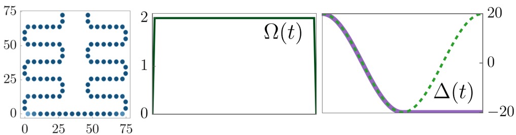
We relate the microscopic origin of dynamical freezing to temporal quantum interference. Such interference naturally arises in periodically driven systems where excitation amplitudes accumulated along distinct time-domain pathways recombine across drive cycles (see Fig. 1(a)).

In effective two-level systems, this process gives rise to Landau–Zener–Stückelberg interference [40, 25, 35, 4, 28, 44, 15, 14, 2, 43, 42]. The extension of this phenomena to large interacting many-body systems remains an open question. Interactions can in principle disrupt the coherent interference underlying dynamical freezing and recent theoretical work has begun to explore this question using simplified interaction models [23, 33]. However, the practical relevance of dynamical freezing hinges on how this interference mechanism behaves in experimentally relevant many-body settings where geometry, interaction strengths and additional couplings substantially modify the freezing conditions.
Programmable Rydberg atom arrays provide a powerful platform to systematically investigate these effects. These systems realize strongly interacting quantum spin models with tunable geometry and long coherence times, enabling exploration of many-body dynamics far beyond few-qubit realizations [3, 13]. They have already enabled discoveries ranging from quantum many-body scars [41] to exotic quantum phases of matter including topological spin liquids [39], quantum critical dynamics and Kibble–Zurek mechanisms [27, 8], quantum optimization [12], and logical qubit encoding [6]. Here we experimentally probe dynamical freezing in programmable Rydberg arrays of up to atoms across one- and two-dimensional geometries. We find that single-frequency driving produces excitation suppression at specific frequencies in a one-dimensional atomic chain, yielding frequency-domain interference fringes (see Fig. 1(b)). Finite-range interaction tails, however, activate interaction-dependent heating channels that already weaken freezing in one dimension and become increasingly detrimental in higher-dimensional geometries.
To overcome this limitation, we introduce dual-parameter modulation of detuning and Rabi frequency that coherently suppresses the dominant heating channels (see Fig. 1(c)). This bifrequency protocol restores and substantially broadens the freezing regime across geometries, producing near-complete excitation suppression even in regimes where conventional driving would strongly heat the system. Combined with a perturbative Floquet framework that incorporates realistic interaction corrections, our results directly reveal how interaction-induced processes destabilize dynamical freezing and demonstrate how these channels can be systematically eliminated. Beyond providing a microscopic understanding of freezing in realistic platforms, our work exposes the limits of idealized Floquet predictions and establishes interference-engineered suppression of heating as a practical route toward stabilizing interacting non-equilibrium quantum matter.
Programmable Rydberg Platform and Drive Protocols
We employ QuEra’s programmable neutral-atom quantum simulator, Aquila, which can host up to 256 Rydberg atoms with flexible geometry. For this work we restrict to systems of approximately 100 atoms. This scale is set jointly by device geometry and the finite probability of preparing defect-free arrays [46].
Each atom is encoded as a two-level system consisting of a stable electronic ground state and a high-energy Rydberg state . The collective vacuum state, corresponds to all atoms in . The system dynamics are governed by the Hamiltonian
| (1) |
where , is the laser detuning, encodes van der Waals interactions between atoms separated by distance , the Rabi frequency.
We probe dynamical freezing via temporal interference under two driving protocols. In the single-frequency case, the detuning is modulated sinusoidally,
| (2) |
In the bi-frequency case, both detuning and Rabi coupling are modulated,
| (3) |
with recovering the single-frequency protocol and introducing a second harmonic that enhances suppression of excitations and visibility of interference pattern. Higher harmonics can also be implemented which produces alternative interference patterns (see Methods). The amplitudes and are chosen such that minima of the measured Rydberg density remain above the SPAM error bound, with visibility and fringe structure controlled systematically by tuning these values.
Dynamical freezing in Rydberg chains


One-dimensional chains provide an ideal setting to uncover the microscopic physics of many-body dynamical freezing arising from temporal interference. We arrange Rydberg atoms in a snake-like configuration with m spacing (Fig. 2, top panels), initialize the system in the vacuum state , and measure the Rydberg excitation density after a single drive cycle. Using and , we observe pronounced oscillations in excitation density as the drive frequency is varied. These frequency-domain oscillations manifest alternating regimes of enhanced excitation and strong dynamical freezing of the vacuum state, arising from temporal interference between dynamical phases accumulated at successive passages through avoided level crossings during a drive cycle. At the first crossing, the system’s wavefunction coherently splits into components evolving along different energy branches, each accumulating a distinct dynamical phase as time progresses. When the system encounters the second crossing, these phases recombine and depending on their relative phase difference, interference can be constructive, yielding enhanced excitation, or destructive, leading to near-complete suppression and hence dynamical freezing.
In our system, the enhanced Rydberg excitation corresponds to the “bright” fringes, while the minima represent strong dynamical freezing of the vacuum. The resulting Stückelberg interference pattern extends coherently across the entire -atom array, demonstrating controllable many-body freezing. To characterize the strength of these fringes we analyze both their visibility and the residual excitation density at the freezing minima.
To quantify the robustness of the freezing fringes we define their visibility across a minima. In Fig. 2(a), at high frequencies (), the fringe achieves , indicating excellent destructive interference and strong dynamical freezing across all atoms. The excitation density at the freezing minimum reaches , approaching the limits set by SPAM errors. As the frequency decreases, however, the contrast drops to at for , and still lower for , while the excitation density at the minima correspondingly increases. This degradation reflects the breakdown of clean Stückelberg interference in the low-frequency regime where additional interaction-induced processes and finite-size effects disrupt coherent phase cancellation. Part of the reduction also arises from the finite s coherence time of the device and due to strong finite size and geometry effects as can be seen in the comparison with experimental data. Nevertheless, the persistence of clear freezing minima confirms the robustness of the underlying interference mechanism in a genuinely interacting ensemble.
Motivated by this degradation of freezing at lower frequencies, we explore whether additional control parameters can stabilize the destructive interference responsible for freezing. We demonstrate how enhanced control is achieved through dual-frequency driving in Fig. 2(c,d). Introducing a bi-frequency modulation, with , provides independent control over both the instantaneous energy gap and the mixing between states at the avoided crossings. This additional handle allows the relative phases accumulated along different dynamical pathways to be tuned more effectively, thereby suppressing excitation channels that would otherwise lead to heating. As a result, excitations are strongly suppressed across the entire frequency range. The suppression is so effective that the excitation density remains close to the noise floor for much of the parameter range; to reveal the residual interference structure within this strongly frozen regime we increase the peak Rabi amplitude from to . Even in the low-frequency regime where single-frequency driving exhibits substantial excitation, the bifrequency protocol maintains strong freezing, demonstrating that multi-parameter control of temporal interference provides a powerful route to stabilizing dynamical freezing in interacting many-body systems.


However, constrained model simulations capture the qualitative structure of the freezing fringes but systematically overestimate the degree of excitation suppression. In particular, when is the ground state at , they predict an additional minimum at that is absent even in small-size blockade simulations. This discrepancy suggests that interaction processes beyond the ideal blockade constraint significantly modify the phase accumulation responsible for dynamical freezing.
We account for these discrepancies using perturbative Floquet theory (see Methods). Within this framework, dynamical freezing occurs when destructive interference suppresses excitation pathways, which happens at frequencies where the leading Bessel-function channel vanishes leading to an emergent conserved total . Constrained models achieve near-ideal freezing by inhibiting competing pathways, while finite-range Rydberg interaction tails activate additional excitation channels, breaking the conservation law strongly or weakly depending on the strength of interaction and frequency. These processes reshape the freezing landscape, explaining the observed detuning asymmetry, fringe shifts, and geometry dependence.
Bi-frequency driving fundamentally alters this structure. Simultaneous detuning and Rabi modulation introduce additional harmonic processes with amplitudes , the characteristic signature of periodically driven quantum systems. When , the second harmonic interferes destructively with the primary excitation channel, enhancing vacuum-state freezing and suppressing the processes that break the emergent conservation law, thereby stabilizing low excitation densities even at low frequencies where single-frequency protocols typically exhibit heating. First-order perturbation theory (see Methods) shows that, at leading order, uniquely produces this destructive interference, while several other ratios do not.
Features governed by lowest-order dynamics, such as the existence of freezing frequencies and the enhancement provided by bifrequency driving, remain robust and universal. In contrast, the precise depth and visibility of freezing minima, as well as geometry-dependent modulation, arise from processes sensitive to the full interaction profile, highlighting how realistic interactions both limit and enable controllable stabilization of dynamical freezing in driven many-body systems.
Interactions reshape the freezing landscape
We next demonstrate how interatomic spacing controls dynamical freezing through Stückelberg interference, revealing finite-range interactions’ decisive role in the freezing landscape (Fig. 3). Unlike constrained models where blockade radius changes negligibly affect interference, the full Rydberg Hamiltonian exhibits marked distance sensitivity from van der Waals tails extending beyond nominal blockade radii.
At our spacings (–m), next-nearest-neighbor interactions remain , which is a regime where interaction and drive energies compete directly, making freezing patterns acutely distance-sensitive. At m, no freezing minimum appears near rads, yet this feature emerges at m in both Bloqade simulations and experiments, albeit with reduced visibility. At m, the strongest dynamical freezing shifts to rads, qualitatively reproduced across and despite decreasing visibility with system size.
This distance sensitivity reveals how finite-range tails continuously reshape the conditions for dynamical freezing as atoms separate, shifting the relative contributions of neighbor couplings and altering phase accumulation. Floquet perturbation theory (see Methods) quantifies this by showing that the interaction corrections to resonances depend explicitly on distance, producing the observed shifts in freezing minima that fixed-blockade models miss entirely.
Complementing geometric control, detuning amplitude provides energetic tuning (Fig. 3(c)). First-order theory predicts freezing at Bessel-function zeros , yielding frequencies scaling with . Experiments confirm this: freezing minima shift systematically to lower frequencies as decreases. However, at sufficiently small , single-frequency driving loses effectiveness and visibility degrades, signaling entry into non-perturbative regimes beyond lowest-order theory where dynamical freezing becomes fragile.
These results establish distance, geometry, and drive parameters as a multidimensional control space for engineering dynamical freezing via temporal interference, providing practical routes to stabilizing quantum states and designing robust Floquet protocols in interacting many-body systems.


Freezing beyond one-dimension
Having established controllable temporal interference and the resulting dynamical freezing in one dimension, we extend to two-dimensional lattices, where atoms interact with multiple neighbors and acquire geometry-dependent phases. These additional pathways provide a stringent test of whether coherent interference and the associated dynamical freezing of the vacuum survives genuine many-body complexity. Moreover, entanglement growth and long-range couplings render tensor-network simulations inefficient in two dimensions, making experimental access particularly valuable. Figure 4 compares square and honeycomb geometries, with Bloqade simulations for benchmarked against Aquila experiments at and numerical results from the constrained model. All data are initialized from the vacuum state with rad/s.
Compared to one-dimensional chains, single-frequency driving exhibits strongly reduced fringe visibility in two dimensions. At , both square and honeycomb lattices retain only a single weak interference minimum, corresponding to a much weaker dynamical freezing point, with strong finite-size effects evident when benchmarked against simulations. The suppression is more pronounced in the honeycomb geometry, particularly at low frequencies where finite coherence further limits contrast. This geometry-dependent degradation reflects the increased role of next-nearest-neighbor interactions and competing interference channels, which hinder precise phase cancellation as connectivity increases, consistent with our analytical framework. By contrast, constrained simulations are insensitive to geometry and dimensionality, reproducing the same behaviour as in one dimension.
Dual-frequency modulation, with rad/s (Fig. 4), restores high-contrast interference. In square lattices, excitation suppression yields a visibility of , corresponding to strong dynamical freezing () of the vacuum, exceeding one-dimensional performance. In honeycomb lattices, bi-frequency driving stabilizes coherent interference patterns from to , where single-frequency modulation fails. The additional Rabi-frequency modulation introduces a secondary temporal interference channel that compensates for the complex next-nearest-neighbor phase network; visibility can be further enhanced by reducing . This stabilization relies on the choice of harmonics. Only certain commensurate drive frequencies reinforce constructive cancellation, while incommensurate combinations induce uncontrolled phase drifts.
These results establish multi-frequency driving as essential for robust dynamical freezing via temporal interference in two dimensions, where complex interaction networks require multiple phase-matching conditions to sustain coherent cancellation.
Microscopic origin of temporal interference
To understand the rich structures observed in the interference patterns and the resulting dynamical freezing landscape, e.g. sensitivity to drive protocol, detuning sign, interaction range, and geometry, we develop an analytical picture based on Floquet perturbation theory over a single drive cycle (see Methods and Appendix. C).
At leading order, the effective Hamiltonian takes the form
| (4) |
where the interaction-dependent coefficient
| (5) |
encodes dynamical phase accumulation during one period. Here represents the interaction-induced energy shift at site , indicates the atoms outside the blockade radius, is the th Bessel function, , and denotes spin-flip operators projected into the blockade-constrained subspace.
This expression provides the microscopic interpretation of temporal interference and the conditions for dynamical freezing. In the non-interacting or perfectly constrained limit (), harmonic contributions recombine destructively over a full cycle, leaving only the channel active. Frequencies satisfying eliminate this channel entirely, producing dynamical freezing. This explains both the emergence of interference minima and why models practically mimic single-particle LZS interference fringes: at low order, the excitation channels are same for both with some suppression via the blockade constraint for model, independent of drive details. Crucially, reversing detuning sign preserves , consistent with the symmetry exhibited by constrained models.
Finite-range interactions open interaction-assisted excitation channels that qualitatively modify the dynamics. When , excitation amplitudes become conditional on surrounding occupations, allowing interactions with nearby Rydberg atoms to enable or suppress spin flips. In a low- expansion of Eq. (5), terms linear in describe these density-assisted processes. This also shows that the stability of dynamical freezing depends on the initial excitation density: states with more pre-existing Rydberg excitations activate more interaction-assisted channels and therefore more readily destabilize freezing. The shifted denominators redistribute spectral weight across harmonics, breaking perfect destructive interference and thereby destabilizing dynamical freezing while generating the detuning asymmetry absent in constrained models. Because depends on both interaction strength and interatomic distance, resonance frequencies shift and fringe visibility degrades when low harmonics approach resonance, activating heating channels and producing the spacing-dependent suppression of freezing observed in Fig. 3.
This framework also clarifies dimensional effects. In two dimensions, each atom couples to multiple neighbors at different distances, broadening the distribution of and introducing competing phase contributions. In square lattices, nearest and next-nearest neighbors remain blockaded, but the next interaction shell at , the one-dimensional next-nearest-neighbor distance, falls within the tail regime, with four such neighbors contributing (compared to two in one dimension), thereby increasing the number of competing excitation channels and reducing fringe visibility. Honeycomb lattices are more fragile: six next-nearest neighbors at distance produce interaction shifts , placing them directly in resonance with the drive and opening strong heating channels that severely suppress interference and hence the freezing observed in experiments.
Bi-frequency driving modifies at leading order by introducing additional harmonic contributions (see Methods). When Rabi modulation frequency equals twice the detuning frequency (), these channels interfere destructively with primary pathways (see Fig. 5 in Methods), suppressing residual excitations and systematically shifting minima due to altered phase-matching conditions. This explains the enhanced freezing and improved low-frequency performance observed experimentally.
Together, this microscopic picture shows that temporal interference in Rydberg arrays is governed by interaction-induced phase redistribution. While lowest-order Floquet theory captures the qualitative structure, higher-order effects become important when interaction tails approach drive energies. Interaction range, geometry, and harmonic content thus provide the key microscopic controls over the emergence and stability of dynamical freezing in driven many-body systems.
Outlook
Our demonstration of controllable many-body dynamical freezing through temporal interference establishes a new paradigm for stabilizing non-equilibrium quantum matter. By strongly suppressing heating and delaying thermalization, dynamical freezing can dramatically extend coherent lifetimes and the retention of many-body memory, attributes valuable for quantum control and information processing in driven systems. Moreover, the bifrequency driving protocols we establish provide practical design principles for stabilizing driven many-body systems beyond what can be achieved using single-frequency protocols. The strong sensitivity of freezing points to sub-micron variations in interatomic spacing also suggests potential applications in precision sensing, where collective Rydberg responses could transduce small interaction changes into measurable shifts of the freezing condition.
Temporal interference, which is the mechanism behind this dynamical freezing, also governs non-adiabatic quantum annealing, where systems traverse avoided crossings at finite speed. By engineering when dynamical phases accumulate or cancel, one can accelerate quantum state preparation while preserving high fidelity, offering advantages beyond conventional adiabatic schemes. In this context, dynamical freezing provides a mechanism for suppressing unwanted excitations during optimization protocols, identifying interference-based control of non-equilibrium dynamics as a general resource for quantum optimization and algorithm design. Recent demonstrations of gate-engineered interference in digital quantum circuits [20] highlight the universality of these ideas across analog and digital architectures.
Finally, our results place the striking dynamical freezing predicted in constrained models into a realistic many-body setting. Dynamical freezing arises from emergent conservation laws that strongly suppress thermalization, producing long-lived non-ergodic dynamics with persistent many-body memory. In idealized PXP descriptions, where the Rydberg blockade is treated as perfect, the Hilbert-space constraint prevents processes that would break these conservation laws, allowing freezing to persist over extremely long timescales. Our experiments show how realistic Rydberg interactions modify this picture: finite-range interaction tails reshape the interference conditions underlying freezing, producing patterns that depart from constrained descriptions and shifting the regimes where stabilization occurs. By systematically controlling geometry, interaction strength and drive protocols, we identify the microscopic mechanisms responsible for these deviations and demonstrate how they can be counteracted through appropriate driving protocols. In this way, our results clarify both the limits of idealized blockade models and practical routes for engineering dynamical freezing in interacting Floquet quantum matter.
Methods
.1 Experimental platform
Experiments were performed on QuEra’s programmable quantum processor, Aquila [46], which traps up to 256 individual 87Rb atoms in reconfigurable optical tweezer arrays. Each atom encodes a qubit between the ground state and a Rydberg state , coupled by a far-detuned two-photon transition (420 nm + 1013 nm). Pairs of Rydberg excitations interact via a van der Waals potential
(calibrated for ). The maximum Rabi frequency which can be used is (corresponding to MHz), which sets a characteristic static blockade radius for zero detuning, i.e. ,
In our driven protocols and vary periodically, so the instantaneous blockade radius is itself time-dependent over the cycle. Unless noted otherwise, quoted blockade values refer to .
Atoms were optically pumped to the state with fidelity exceeding before each experimental run. Finite site-loading imperfections introduce an average defect probability of per site. Thus it is expected that we obtain defect-free configurations in approximately of attempts for -atom arrays [46], subject to some corrections based on geometry. All reported data were obtained exclusively from verified defect-free realizations, identified via fluorescence imaging. To visualize geometry-dependent trapping reliability, the probability of successful atom loading is indicated by graded colour shading in the geometry figures shown in the main text. To ensure uniformity while maintaining experimental efficiency, we restrict all measurements to arrays containing atoms across one- and two-dimensional geometries.
One-dimensional “snake” chains were limited by the active region of the device. At an interatomic spacing of m, up to atoms could be accommodated; increasing to and m reduced the usable system size to 88 and 84, respectively. Two-dimensional square and honeycomb arrays of comparable scale were realized under interatomic spacing of as well.
.2 Drive protocols
Time-dependent control of the detuning and Rabi frequency was implemented using piecewise-linear waveforms with 50 ns temporal resolution. We employed two primary protocols:
| (6) |
where (single-frequency) modulates only detuning with constant Rabi amplitude , and (dual-frequency) adds a commensurate Rabi modulation.
Drive angular frequencies spanned –, with most data taken between and so that single-cycle durations remain within the system coherence window reported in Aquila whitepaper [46]. Each cycle began and ended at , with ns rise and fall times set by hardware constraints.
A practical limitation at higher is the fixed rise and fall overhead in . Each cycle includes ns ramps at both the beginning and end, amounting to a total overhead of s per period. The fractional time spent ramping,
increases linearly with drive frequency. Consequently, around of each cycle is consumed by ramps at , rendering still higher frequencies inefficient. Most experiments were therefore restricted to , where the effective portion of the cycle used for coherent evolution exceeds .
Typical control amplitudes were – and , unless otherwise stated. All measurements report the Rydberg population after exactly one complete drive cycle ().
.3 Measurement and error correction
Rydberg state populations were measured via fluorescence detection after each drive sequence, averaging at least defect-free shots per data point (corresponding to total attempts depending on loading probability). State-preparation and measurement (SPAM) errors were corrected using calibrated values (false ground detection) and (false Rydberg detection) [46]:
| (7) |
Error bars in figures represent standard error of the mean computed from shot-to-shot fluctuations. Nearest-neighbour interatomic distances were uniform within each geometry to within nm, except at snake-pattern bends where natural geometric variations occur.
.4 Analytical understanding
To develop a microscopic understanding of the observed interference dynamics, we derive the effective Floquet Hamiltonian governing evolution over a single drive cycle. While alternative approaches, such as explicit LZS phase accumulation or rotating-wave approximations, can describe isolated avoided crossings, the Floquet Hamiltonian method offers a simple and physically transparent route to characterize excitation dynamics over one complete driving period.
Exact calculation of the Floquet Hamiltonian, , is intractable for large interacting systems such as Rydberg arrays (and even nontrivial for a single qubit under our protocol). We therefore adopt a perturbative expansion formulated in the interaction picture, a resummed variant of the standard Floquet–Magnus expansion that remains accurate even at intermediate drive frequencies, the Floquet perturbation theory [16]. We decompose the Hamiltonian as
| (8) |
where acts as a perturbation to . Both terms may retain explicit time dependence; accuracy and convergence of the expansion depends on their relative energy scales as discussed in Ref. 16.
For our driven Rydberg system, we define, , with
| (9) | ||||
| (10) |
Here denotes the set of sites outside the blockade radius that interact with site , and denotes a spin-flip operator projected into the Rydberg blockade subspace, where enforces the constraint that no two excitations occur within the blockade radius . Nearest-neighbour interactions are not included explicitly in and are instead incorporated implicitly through the projection operator in , as their magnitude far exceeds all other energy scales in the problem. Their effect is to energetically suppress configurations with neighbouring excitations, allowing the dynamics to be accurately captured by projection into the blockade subspace. The blockade radius is defined operationally as the distance below which the interaction energy exceeds the drive and detuning scales. Crucially, while interactions within are integrated out by the projection, we explicitly retain the long-range interaction tails beyond , the blockade radius through the couplings , which provide the leading corrections to the PXP description and underpin the interaction-induced dynamics discussed here. Depending on the lattice geometry and interatomic spacing, this projection may exclude different sets of neighbouring sites.
Relegating the detailed calculations and explanations to Appendix C, we state the effective Floquet Hamiltonian in the leading orders of perturbation theory as,
| (11) |
| (12) |
with
| (13) |
For , the coefficient can be expanded to leading order as
| (14) |
and thus
| (15) | ||||
where
| (16) |
The above analysis generalizes directly to an amplitude-modulated transverse drive , with integer . Up to first order in the interaction-picture expansion, the effective Floquet Hamiltonian is
| (17) |
where and
| (18) |
In the regime , the coefficient appearing in the first-order Floquet Hamiltonian for the bifrequency drive admits an expansion of the form
| (19) |
with
| (20) |

For even , the additional resonant contribution proportional to modifies the bare flip amplitude, whereas for odd this contribution vanishes identically, see Fig. 5 for some representative values of .
Data availability:
The data that support the findings of this study are available at https://doi.org/10.5281/zenodo.18482467
Code availability:
The codes used for the simulations and analysis in this study are available at https://doi.org/10.5281/zenodo.18482467.
Acknowledgements.
This research used resources of the National Energy Research Scientific Computing Center (NERSC), a Department of Energy Office of Science User Facility under Contract No. DE-AC02-05CH11231 using NERSC award for QCAN Project DDR-ERCAP0033861. This project was also funded and supported by the UK National Quantum Computer Centre [NQCC200921], which is a UKRI Centre and part of the UK National Quantum Technologies Programme (NQTP). SB, MS and RG acknowledge EPSRC-SFI funded project EP/X039889/1 (GeQuantumBus). BZ was supported by the Engineering and Physical Sciences Research Council [grant numbers EP/R513143/1, EP/T517793/1]. B. M. was funded by Department of Science & Technology, Government of India via the INSPIRE Faculty programme. B.M was also funded by the European Research Council (ERC) under the European Union’s Horizon 2020 research and innovation programme (Grant Agreement No. 853368), near the beginning of this project. The authors would like to thank Pedro Lopez, Milan Kornjača, Katherine Klymko and other members of the QuEra-NERSC team for discussions. RG and MS would like to thank Krishnendu Sengupta, Arnab Sen and Alexander Nico-Katz for discussions. BM would like to thank Krishnendu Sengupta and Dolev Bluvstein for discussions.References
- [1] (2015-12) Exponentially slow heating in periodically driven many-body systems. Phys. Rev. Lett. 115, pp. 256803. External Links: Document, Link Cited by: Introduction.
- [2] (2022-05) All-optical stückelberg spectroscopy of strongly driven rydberg states. Phys. Rev. Res. 4, pp. 023135. External Links: Document, Link Cited by: Introduction.
- [3] (2017-11) Probing many-body dynamics on a 51-atom quantum simulator. Nature 551 (7682), pp. 579–584. External Links: Link, Document Cited by: Introduction.
- [4] (2006-10) Coherent quasiclassical dynamics of a persistent current qubit. Phys. Rev. Lett. 97, pp. 150502. External Links: Document, Link Cited by: Introduction.
- [5] (2021) Controlling quantum many-body dynamics in driven rydberg atom arrays. Science 371 (6536), pp. 1355–1359. External Links: Document, Link, https://www.science.org/doi/pdf/10.1126/science.abg2530 Cited by: Introduction.
- [6] (2023-12) Logical quantum processor based on reconfigurable atom arrays. Nature 626 (7997), pp. 58–65. External Links: Link, Document Cited by: Introduction.
- [7] (2015) Universal high-frequency behavior of periodically driven systems: from dynamical stabilization to floquet engineering. Advances in Physics 64 (2), pp. 139–226. External Links: Document, Link, https://doi.org/10.1080/00018732.2015.1055918 Cited by: Introduction.
- [8] (2025) Probing emergent prethermal dynamics and resonant melting on a programmable quantum simulator. External Links: 2510.11706, Link Cited by: Introduction.
- [9] (2010-11) Exotic freezing of response in a quantum many-body system. Phys. Rev. B 82, pp. 172402. External Links: Document, Link Cited by: Introduction.
- [10] (2020-05) Floquet engineering topological many-body localized systems. Phys. Rev. Lett. 124, pp. 190601. External Links: Document, Link Cited by: Introduction.
- [11] (2024-06) Floquet-rydberg quantum simulator for confinement in gauge theories. Phys. Rev. Res. 6, pp. L022059. External Links: Document, Link Cited by: Introduction.
- [12] (2022-06) Quantum optimization of maximum independent set using rydberg atom arrays. Science 376 (6598), pp. 1209–1215. External Links: Link, Document Cited by: Introduction.
- [13] (2021-07) Quantum phases of matter on a 256-atom programmable quantum simulator. Nature 595 (7866), pp. 227–232. External Links: Link, Document Cited by: Introduction.
- [14] (2014-03) Characterization of qubit dephasing by landau-zener-stückelberg-majorana interferometry. Phys. Rev. Lett. 112, pp. 116803. External Links: Document, Link Cited by: Introduction.
- [15] (2011-11) Geometric landau-zener interferometry. Phys. Rev. Lett. 107, pp. 207002. External Links: Document, Link Cited by: Introduction.
- [16] (2020-12) Floquet perturbation theory for periodically driven weakly interacting fermions. Phys. Rev. B 102, pp. 235114. External Links: Document, Link Cited by: Appendix C, 4.§, 4.§.
- [17] (2018-01) Ramp and periodic dynamics across non-ising critical points. Phys. Rev. B 97, pp. 014309. External Links: Document, Link Cited by: §D.1, Appendix D, Introduction.
- [18] (2025) Destructive interference induced constraints in floquet systems. arXiv preprint arXiv:2508.18368. Cited by: Introduction.
- [19] (2023-03) Prethermal fragmentation in a periodically driven fermionic chain. Phys. Rev. Lett. 130, pp. 120401. External Links: Document, Link Cited by: Introduction.
- [20] (2025-10-22) Observation of constructive interference at the edge of quantum ergodicity. Nature. External Links: ISSN 1476-4687, Document, Link Cited by: Outlook.
- [21] (2025-06) Dynamical freezing in exactly solvable models of driven chaotic quantum dots. Phys. Rev. Lett. 134, pp. 226501. External Links: Document, Link Cited by: Introduction.
- [22] (2024) Dynamical freezing in the thermodynamic limit: the strongly driven ensemble. External Links: 2410.11050, Link Cited by: Introduction.
- [23] (2021-04) Dynamical freezing and scar points in strongly driven floquet matter: resonance vs emergent conservation laws. Phys. Rev. X 11, pp. 021008. External Links: Document, Link Cited by: Introduction, Introduction.
- [24] (2025-06-06) Floquet amorphous topological orders in a one-dimensional rydberg glass. Communications Physics 8 (1), pp. 237. External Links: ISSN 2399-3650, Document, Link Cited by: Introduction.
- [25] (2023) Nonadiabatic landau–zener–stückelberg–majorana transitions, dynamics, and interference. Physics Reports 995, pp. 1–89. Note: Nonadiabatic Landau-Zener-Stückelberg-Majorana transitions, dynamics, and interference External Links: ISSN 0370-1573, Document, Link Cited by: Introduction.
- [26] (2016-08) Tuning towards dynamic freezing using a two-rate protocol. Phys. Rev. B 94, pp. 075130. External Links: Document, Link Cited by: Introduction.
- [27] (2019-04) Quantum kibble–zurek mechanism and critical dynamics on a programmable rydberg simulator. Nature 568 (7751), pp. 207–211. External Links: Link, Document Cited by: Introduction.
- [28] (2019-12) Landau-zener-stückelberg interference in a multimode electromechanical system in the quantum regime. Phys. Rev. Lett. 123, pp. 240401. External Links: Document, Link Cited by: Introduction.
- [29] (2016-06) Phase structure of driven quantum systems. Phys. Rev. Lett. 116, pp. 250401. External Links: Document, Link Cited by: Introduction.
- [30] (2015-07) Fate of many-body localization under periodic driving. Phys. Rev. Lett. 115, pp. 030402. External Links: Document, Link Cited by: Introduction.
- [31] (2020-06) Collapse and revival of quantum many-body scars via floquet engineering. Phys. Rev. B 101, pp. 245107. External Links: Document, Link Cited by: Introduction.
- [32] (2020-08) Dynamics of the vacuum state in a periodically driven rydberg chain. Phys. Rev. B 102, pp. 075123. External Links: Document, Link Cited by: Introduction.
- [33] (2026-02) Floquet thermalization via instantons near dynamical freezing. Phys. Rev. X 16, pp. 011041. External Links: Document, Link Cited by: Appendix B, Introduction.
- [34] (2019) Floquet engineering of quantum materials. Annual Review of Condensed Matter Physics 10 (1), pp. 387–408. Cited by: Introduction.
- [35] (2005) Mach-zehnder interferometry in a strongly driven superconducting qubit. Science 310 (5754), pp. 1653–1657. External Links: Document, Link, https://www.science.org/doi/pdf/10.1126/science.1119678 Cited by: Introduction.
- [36] (2021-04-01) Floquet prethermalization in dipolar spin chains. Nature Physics 17 (4), pp. 444–447. External Links: ISSN 1745-2481, Document, Link Cited by: Introduction.
- [37] (2015-04) Many-body localization in periodically driven systems. Phys. Rev. Lett. 114, pp. 140401. External Links: Document, Link Cited by: Introduction.
- [38] (2021-05) Mobility edge and multifractality in a periodically driven aubry-andré model. Phys. Rev. B 103, pp. 184309. External Links: Document, Link Cited by: Introduction.
- [39] (2021-12) Probing topological spin liquids on a programmable quantum simulator. Science 374 (6572), pp. 1242–1247. External Links: Link, Document Cited by: Introduction.
- [40] (2010) Landau–zener–stückelberg interferometry. Physics Reports 492 (1), pp. 1–30. External Links: ISSN 0370-1573, Document, Link Cited by: Introduction.
- [41] (2018-07-01) Weak ergodicity breaking from quantum many-body scars. Nature Physics 14 (7), pp. 745–749. External Links: ISSN 1745-2481, Document, Link Cited by: §D.1, Introduction.
- [42] (2009-12) Observation of stückelberg oscillations in dipole-dipole interactions. Phys. Rev. A 80, pp. 063407. External Links: Document, Link Cited by: Introduction.
- [43] (2025-10-09) Electrically tunable quantum interference of atomic spins on surfaces. Nature Communications 16 (1), pp. 8988. External Links: ISSN 2041-1723, Document, Link Cited by: Introduction.
- [44] (2020-08) Landau-zener-stückelberg-majorana interferometry of a superconducting qubit in front of a mirror. Phys. Rev. B 102, pp. 075448. External Links: Document, Link Cited by: Introduction.
- [45] (2025-09-01) Probing non-equilibrium topological order on a quantum processor. Nature 645 (8080), pp. 348–353. External Links: ISSN 1476-4687, Document, Link Cited by: Introduction.
- [46] (2023) Aquila: quera’s 256-qubit neutral-atom quantum computer. External Links: 2306.11727, Link Cited by: Programmable Rydberg Platform and Drive Protocols, 1.§, 1.§, 2.§, 3.§.
- [47] (2023-11-06) Floquet-tailored rydberg interactions. Nature Communications 14 (1), pp. 7128. External Links: ISSN 2041-1723, Document, Link Cited by: Introduction.
Author contributions:
B.Z. prepared the experiments in QuEra Aquila, which were jointly performed by R.G., M.S. and B.Z. M.S. performed the data analysis and generated the figures. M.S. and R.G. carried out the analytical calculations, while M.S. and B.M. performed the numerical computations. The project was conceived during discussions among S.B., R.G., B.M. and M.S.. R.G. co-ordinated the experimental, numerical and theoretical components of the work. All authors contributed to writing the manuscript.
Competing Interests:
The authors declare no competing interests.
Appendix A Resolving interference within individual drive cycles


The frequency-dependent vacuum freezing raises a fundamental question: how do quantum phases interfere across repeated passages to produce dynamical stability? To probe this microscopically, we track the time-resolved Rydberg population within a single drive cycle in 100-atom chains on Aquila (Fig. 6), benchmarked against Bloqade simulations at .
At frequencies yielding destructive interference (), the excitation probability rises approaching the first avoided crossing but falls during the second, completing the cycle with —near-perfect vacuum recovery. In contrast, at constructive frequencies (), excitations accumulate coherently across both traversals, leading to final densities exceeding .
To confirm that interference requires completion of the full temporal loop, we implement a truncated protocol halting evolution at half-period (), keeping fixed thereafter. In this case, the characteristic contrast vanishes. Excitation grows monotonically and settles into residual oscillations, demonstrating that the observed freezing originates from phase recombination across the full cycle, not from single-pass dynamics.
These time-resolved measurements directly visualize the Stückelberg mechanism at the many-body level. By resolving constructive and destructive recombination within each drive cycle of a -atom ensemble, our results establish temporal interference as a coherent, scalable mechanism underlying Floquet control in interacting quantum systems.
Appendix B Interference after multiple drive cycles


In this section we report the excitation density under repeated periodic driving. To remain within the experimentally accessible coherence time, we consider higher drive frequencies than in the main text and focus on parameters near the first (smallest) zero of the Bessel function . Since the argument of scales as , this corresponds to the highest drive frequency at which the characteristic interference minima remain observable in our experiment. We experimentally measure the excitation density for atoms in a snake geometry after two and four drive cycles, shown in Fig. 7 (left and right panels, respectively), and compare these results with numerical simulations obtained using Bloqade for a system of size , as well as with the constrained PXP model at the same size.
While temporal interference persists over multiple cycles, its visibility is significantly reduced with increasing drive duration. In particular, the excitation density at points of constructive interference is markedly higher after four cycles than after two, indicating the onset of Floquet heating. This behavior is captured both in experiment and in the full Rydberg simulations, consistent with the understanding that dynamical freezing in interacting Floquet systems is generally a transient prethermal regime rather than a truly stable phase, in line with recent theoretical studies attributing such heating processes to instanton-mediated mechanisms [33].
By contrast, the model exhibits substantially weaker degradation of interference visibility over the same timescales, reflecting its effectively constrained and non-generic interaction structure. This comparison highlights that finite-range interaction tails play a central role in enabling genuine many-body dynamics and in determining the long-time stability of driven interference phenomena. In this sense, the extended interactions present in realistic Rydberg systems are not merely a perturbation to constrained models but are essential for capturing the experimentally observed heating and coherence properties.
Appendix C The Floquet Perturbation expansion
In the main text we define, For our driven Rydberg system, we define, , with
| (21) | ||||
| (22) |
The Floquet perturbation expansion proceeds analogously to a Dyson series formulated in the interaction picture [16]. The zeroth-order term defines the unperturbed evolution operator
| (23) |
where denotes time ordering. Since is diagonal at all times, the corresponding zeroth-order evolution operator is obtained exactly as
| (24) |
The zeroth-order contribution to the Floquet Hamiltonian arises from the evolution operator over one driving period. Since for , the contribution from the time-dependent detuning vanishes over a full period, and one finds
| (25) |
This defines the zeroth-order Floquet Hamiltonian
| (26) |
which corresponds to the static interaction energy within the blockade-constrained Hilbert space.
To calculate the first order term, we start from the interaction-picture Hamiltonian
| (27) |
which takes the form
| (28) |
with
| (29) |
Here are projected spin-flip operators acting within the blockade subspace. The quantity is diagonal in the occupation-number basis and therefore commutes with itself at different times, allowing it to be treated as a c-number within the time integral. The effective Floquet Hamiltonian is then defined in the interaction frame generated by . Transforming back to the laboratory frame yields , where is diagonal in the occupation basis and contributes only configuration-dependent phases, leaving the effective coupling structure unchanged.
First-order Dyson expansion
The time-evolution operator in the interaction picture is
| (30) |
where denotes time ordering. To first order in the Dyson expansion, this reduces to
| (31) |
The effective Floquet Hamiltonian at this order is defined through
| (32) |
which yields
| (33) |
Evaluation of the time integral
To evaluate Eq. (35), we employ the Jacobi–Anger expansion
| (36) |
This allows us to write
| (37) |
Substituting into Eq. (35), we obtain
| (38) |
The remaining time integral can be evaluated explicitly as
| (39) |
Using and the identity , this simplifies to
| (40) |
Combining terms yields the closed-form expression
| (41) |
which corresponds to Eq. (12) in the main text.
Physical interpretation
Since depends only on occupations outside the blockade radius, the coefficient conditions the spin-flip dynamics at site on the surrounding Rydberg configuration. The resulting effective Hamiltonian therefore describes density-assisted spin-flip processes arising from interaction tails beyond the blockade radius.
Small-interaction expansion of the Floquet Hamiltonian
We now consider the regime in which interactions beyond the blockade radius are weak but finite,
| (42) |
which allows us to expose the effect of interaction tails while remaining controlled by the large detuning scale. In this limit, interaction-induced corrections arise in the effective Floquet Hamiltonian that are absent in the PXP model.
Up to first order in the interaction-picture Dyson expansion, the effective Floquet Hamiltonian can be written as
| (43) |
where the zeroth-order contribution originates entirely from the diagonal part of the Hamiltonian retained in ,
| (44) |
The first-order contribution arises from the time average of the interaction-picture Hamiltonian and is controlled by the coefficient
| (45) |
In the present regime, the interaction-induced shift
| (46) |
satisfies , allowing to be expanded perturbatively in .
Using the Jacobi–Anger expansion and expanding the integrand to linear order in , we obtain
| (47) | ||||
| (48) |
The first term evaluates to the zeroth-order Bessel function,
| (49) |
while the second term can be evaluated by inserting the Jacobi–Anger expansion and performing the time integral term by term, yielding
| (50) |
Combining these results, the coefficient admits the expansion
| (51) |
Substituting this expression into the first-order Floquet Hamiltonian yields
| (52) |
where the interaction-induced coupling is given by
| (53) |
This expression makes explicit that, even for weak interaction tails, the effective Floquet Hamiltonian acquires density-assisted spin-flip terms that are absent in the PXP model and arise solely from interactions beyond the blockade radius.
The leading interaction-induced correction therefore corresponds to a density-assisted spin-flip process: a spin at site can flip only in the presence of a finite interaction-induced energy shift generated by Rydberg excitations at neighbouring sites beyond the blockade radius. In this regime, interactions do not merely renormalize the global flip amplitude, but condition local spin dynamics on the surrounding Rydberg configuration. Such density-assisted processes are absent in the PXP model and provide the leading correction required to capture the experimentally observed dynamics when interactions beyond the blockade radius are retained.
Dual-frequency drive
We now generalize the above analysis to an rabi-frequency modulated transverse drive of the form
| (54) |
The interaction-picture Hamiltonian becomes
| (55) |
where is defined as in Eq. (S29),
| (56) |
To first order in the interaction-picture Dyson expansion, the effective Floquet Hamiltonian is given by the time average
| (57) |
Substituting the expression for and performing the time average yields
| (58) |
with
| (59) |
To evaluate this integral, we again employ the Jacobi–Anger expansion
| (60) |
Using , Eq. (59) becomes
| (61) | ||||
| (62) |
Each time integral can be evaluated explicitly as
| (63) |
which, using and for integer , simplifies to
| (64) |
Collecting terms, we arrive at the closed-form expression
| (65) |
which reduces to the single-frequency result for .
Remarks
The amplitude modulation introduces additional near-resonant denominators at , allowing multiple Floquet channels to contribute to the effective spin-flip amplitude. As discussed in the main text, this structure enables both enhancement and suppression of the effective transverse dynamics depending on the parity of and the value of .
In the regime , the coefficient appearing in the first-order Floquet Hamiltonian for the bifrequency drive admits an expansion of the form
| (66) |
with
| (67) |
and
| (68) |
As a result, the effective Floquet Hamiltonian contains a drive-renormalized constrained spin-flip term together with an interaction-induced density-assisted correction at linear order in .
Appendix D Numerical simulations
Numerical benchmarks for system sizes – employed two complementary approaches. Full quantum dynamics under the Rydberg Hamiltonian (Eq. 1 of main text) were computed using Bloqade, an open-source python package from QuEra for simulating neutral-atom quantum processors. Simulations retained the complete van der Waals interaction between all atom pairs and employed identical time-discretized drive protocols as experiments.
For comparison with constrained models, we implemented PXP-type Hamiltonians that project out nearest-neighbor Rydberg excitations. Two variants were considered: PXP, which forbids only nearest-neighbor double occupancy, and extended-PXP (PPXPP), which additionally constrains next-nearest neighbors [17]. Time evolution employed second-order Trotterization with 400 steps per drive cycle, yielding relative errors below . All simulations discussed in the main text employed open boundary conditions matching experimental geometries. Thus only parity symmetry was exploited to reduce computational cost, no other approximations were imposed.
However, system sizes up to were numerically accessible for certain geometries, boundary conditions, and parameter regimes, and we present representative results in these regimes in this section. We note that in some parameter regimes, simulations predict excitation densities below at destructive interference points. In such cases, experimental state preparation and measurement (SPAM) errors () would dominate the signal. The parameters presented in the main text were therefore chosen to balance interference visibility with experimental observability, typically ensuring at destructive minima.
D.1 Initial state dependence
In this section, we investigate the dependence of temporal freezing on the choice of initial state. This provides a further probe of the genuinely many-body character of the phenomenon, as the system response is no longer determined solely by the drive protocol but also by the structure of correlations encoded in the initial state. We restrict attention here to exact numerical simulations within the constrained model, which allows us to systematically explore a range of highly nontrivial initial conditions. Experimental implementation of such state-dependent protocols is left for future work.
Complementing the vacuum state considered in the main text, we study the following three initial states:
| Single Rydberg excitation | ||||
| Néel state | ||||
| (69) |
The state is well known to exhibit quantum many-body scar (QMBS)-induced long-lived oscillations of local observables [41]. The state displays similar behavior, albeit with reduced coherence, and can be prepared as the ground state of a Rydberg Hamiltonian with large negative detuning and blockade radius equal to two lattice spacings, a regime associated with non-Ising critical points [17].
In Fig. 8 we plot , where , together with the excitation density as functions of drive frequency for all three initial states. Minima of correspond to strongest freezing. For the single-excitation state , the locations of the freezing points closely match those found for the vacuum state. By contrast, the and states exhibit maxima of at the same frequencies, reflecting a qualitatively different response to the drive.
For the state this behavior is expected, as it already maximizes the allowed Rydberg excitation density within the constrained Hilbert space. The response of the state is more subtle, since the drive does not generate states with higher excitation density. In both these scenarios the dynamical freezing manifests through enhanced fidelity. Overall, these results demonstrate that temporal freezing and its enhancement under bifrequency driving persist well beyond the vacuum sector, with the precise locations and strengths of freezing depending weakly but systematically on the initial state. Interestingly, the fidelity at freezing points is often higher for the correlated initial states considered here than for the vacuum, suggesting that initial many-body correlations can further stabilize interference-induced freezing. The experimental realization of such correlated initial states requires substantial additional preparation overhead and was therefore not pursued in the present work.

D.2 Dependence on system size, boundary conditions and ratio of drive frequencies
In this section we examine the robustness of the freezing phenomenon with respect to system size, boundary conditions, and the ratio of the two drive frequencies. To access larger system sizes within exact diagonalization, we exploit all available lattice symmetries, resolving translations along both spatial directions, reflections about the and axes, and inversion with respect to the diagonal of the square lattice. This symmetry resolution reduces the effective Hilbert space dimension by a factor of order . For instance, restricting to the sector , , , , yields a matrix of dimension 9702 for a lattice, compared to a full constrained Hilbert space dimension of .
We find that increasing system size leads to both a slight shift of the freezing minima toward higher frequencies and a reduction in the overall degree of freezing, as illustrated by the comparison between and lattices in Fig. 9 (left panel). This trend suggests that finite-size effects play a quantitative role in stabilizing interference-induced freezing, while the fate of the phenomenon in the thermodynamic limit remains an open question.
We further observe that the locations of the freezing minima are insensitive to the choice of boundary conditions, as shown in Fig. 9 (middle panel). This is encouraging from an experimental perspective, as open boundary conditions are most naturally implemented in current quantum simulation platforms. Finally, we investigate the dependence on the ratio of the two drive frequencies (Fig. 9, right panel). Among the cases studied, is distinguished by consistently higher fidelity over a broad frequency range, indicating a particularly robust interference condition. A deeper microscopic understanding of why is particularly robust, beyond the effective Bessel interference picture presented here, remains an open direction for future theoretical work.


Appendix E Excitation density distribution

In the main text we characterized the system response using the Rydberg excitation density averaged over all atoms in a particular configuration as a function of the driving frequency. This global observable efficiently captures the emergence of non-equilibrium interference effects, including the appearance of freezing points and enhanced excitation regimes, and allows for a direct comparison across different system geometries and driving protocols. However, such spatial averaging necessarily masks the underlying site-resolved structure of the many-body excitation patterns that develop during the driven dynamics.
Here, we therefore complement the averaged analysis by presenting the local Rydberg excitation probability of each individual atom different lattice geometries and driving protocols. Fig. 10 (a),(b) corresponds to single- and bi-frequency driving for one-dimensional chains (represented by the snake configuration). The bi-frequency driving for two-dimensional square and hexagonal geometries are shown in Fig. 10 (c) and (d) respectively. We choose two representative driving frequencies for Fig. 10(a,b,c,d): (i) frequencies corresponding to the freezing points (left), and (ii) frequencies at which the total excitation density is maximized (right). Fig. 11 represents the effect of changing the interatomic distance for the same geometry at . By resolving the excitation distribution at the single-site level, we demonstrate that the observed extrema in the averaged excitation are not the result of localized or edge-dominated effects, but instead arise from a highly coherent and spatially homogeneous excitation pattern across the entire atomic configuration.
At both the freezing points and the excitation maxima, the site-resolved excitation probabilities remain approximately uniform across most atoms. Modest deviations are observed in regions of local geometric variation, such as near the bends of the snake-like configuration. These deviations do not result in any abrupt redistribution of the overall excitation density toward higher or lower values.
The observed spatial variations arise from interaction effects and reflect local geometric constraints. Their systematic presence across different geometries and driving protocols indicates that the non-equilibrium features discussed in the main text are collective in origin rather than dominated by local inhomogeneities. The site-resolved data therefore support the interpretation of these features as global many-body effects in driven Rydberg systems.
