From Decision Trees to Boolean Logic: A Fast and Unified SHAP Algorithm

Decision trees are widely used predictive models for classification and regression. To improve predictive accuracy, ensemble methods such as XGBoost (Chen and Guestrin 2016), Random Forest (Breiman 2001), and CatBoost (Dorogush et al. 2017), train multiple decision trees and average their predictions.

Recent efforts focus on explaining models using feature attributions. Local attribution shows how each feature affects a single prediction, which is often crucial for regulatory compliance (Knight 2019; Selbst and Powles 2017). Global attribution evaluates which features matter most overall, often by combining many local attributions (Covert et al. 2020). This is essential for model comprehension and feature selection.

SHAP (SHapley Additive exPlanations) (Lundberg et al. 2020) is a widely preferred method for both local and global feature attribution (Gill et al. 2020; Hall and Gill 2019). It assigns Shapley values to features, providing a unified (Lundberg and Lee 2017) and consistent (Lundberg et al. 2019) approach grounded in game theory.

Towards defining WDNF, we need additional notations. A literal is a Boolean variable $x_{i}$ or its negation $\neg x_{i}$. A cube is a conjunction (set) of literals.

For instance, the PB formula $F(x_{1},x_{2},x_{3})=3(\neg x_{1})+1(\neg x_{1}\land x_{2})+5(x_{1}\land\neg x_{2}\land x_{3})$ is in WDNF. Assigning $x_{1}=0$, $x_{2}=1$, $x_{3}=1$ results in $F(0,1,1)=3+1=4$.

For a cube $c_{k}$, we denote by $S_{k}$ the set of variables in $c_{k}$, partitioned into positive variables $S^{+}_{k}$ and negated variables $S^{-}_{k}$. For example, in the cube $c_{k}\equiv x_{1}\land\lnot x_{2}\land x_{3}$, we have $S^{+}_{k}=\{x_{1},x_{3}\}$ and $S^{-}_{k}=\{x_{2}\}$.

A WDNF formula, and any other PB function, can be interpreted as a game where variables are players and the formula’s output is the profit (Grabisch and Roubens 1999). The characteristic function (recall Def. 1) of this game is defined by Def. 3. To find the profit of a coalition $S$, we set $x_{i}=1$ for all $i\in S$, $x_{i}=0$ for all $i\notin S$, and evaluate the WDNF formula. See Fig. 1 for an illustration.

Having defined the characteristic function for a WDNF formula $F$, we can now compute its Shapley values via Formula 1. In general, computing Shapley values for pseudo-Boolean functions is #P-Hard (see Appendix B.5). A key insight of this paper is that, for WDNF, Shapley values can be computed in linear time using the following formula:

Prior to evaluating Formula 2 and the formulas presented in Sect 3, we remove all cubes where $S^{+}_{k}\cap S^{-}_{k}\neq\emptyset$ as such cubes are unsatisfiable. In Appendix B, we prove that Formula 2 correctly computes the Shapley values. The proof leverages the linearity and the null player out (NPO) properties of Shapley values. Additionally, we show how Formula 2 can be computed in linear time and applied to Weighted Conjunctive Normal Form (WCNF) formulas (da Silva 2021).

In this section, we present formulas that efficiently compute the Shapley interaction values $\phi_{i,j}$ (Table 1), Banzhaf values $\beta_{i}$, and Banzhaf interaction values $\beta_{i,j}$ over WDNFs. Proofs of correctness appear Appendix C.

Shapley interaction values measure how the interaction between two features affects the prediction (Grabisch and Roubens 1999). One possible definition is:

By combining Formula 2 with Def. 4, we can derive simple formulas for Shapley interaction values, see Table 1 for further details:

Banzhaf values satisfy three of Shapley’s four properties: null player, symmetry, and linearity. However, they do not satisfy efficiency (Banzhaf 1965). They also possess another useful property: the Banzhaf value of player $i$, equals the difference in the expected game’s profit, under a uniform distribution over all subsets, with and without $i$:

Previous work has shown how to calculate Banzhaf values on decision trees (Karczmarz et al. 2022; Muschalik et al. 2024), facts in query answering (Abramovich et al. 2023), and on other tasks. The formula below enables their linear-time computation on a WDNF formula:

Banzhaf interaction values examine the difference in expectations when feature $i$ and $j$ are both missing/participating versus when only one participates (Fujimoto et al. 2006). Given a WDNF they be computed using the formula below:

This section introduces the concept of a decision pattern, central to Woodelf. We begin by defining decision trees and root-to-leaf paths, and then build on these foundations to define decision patterns and present the efficient CalcDecisionPatterns algorithm for computing them.

In Fig. 2, the ‘Consumer Pattern’ and ‘Baseline Pattern’ columns illustrate how the decision patterns are computed.

Let $C$ be the consumer data matrix with rows $c\in C$, and define $n.\text{split}(C)=(n.\text{split}(c))_{\forall c\in C}$.

Given a decision tree $T$ with $L$ leaves and consumer data $C$ of size $n$, CalcDecisionPatterns (Alg. 1) traverses $T$ using Breadth-First Search (BFS), applying Def. 7 at each node. Running in $O(nL)$ time, it returns a dictionary $P$ mapping each leaf $l_{j}\in L_{T}$ to its consumer decision patterns, where $P[l_{j}][c_{i}]$ stores the pattern for consumer $c_{i}\in C$ at leaf $l_{j}$.

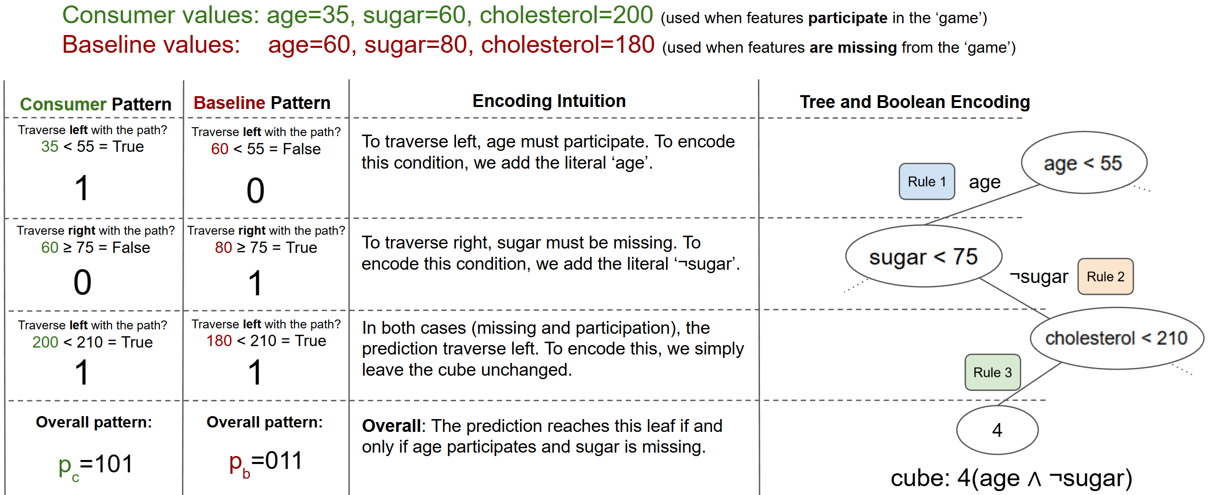
Our baseline SHAP algorithm constructs a WDNF formula $F$ representing the model’s characteristic function. An illustration of this construction is provided in Fig. 2. The variables in $F$ correspond to model features, and each cube captures the contribution of a single leaf. A variable $f_{i}$ set to 1 indicates the feature is present (i.e., set to the consumer’s value $c[f_{i}]$), while 0 denotes a missing feature (i.e., set to the baseline value $b[f_{i}]$). A cube is satisfied if and only if the prediction reaches its corresponding leaf:

We present four simple rules for constructing the WDNF formula. Our goal is to construct a cube that represents a leaf $l$, a consumer $c$, and a baseline $b$. We first run CalcDecisionPatterns to obtain the consumer decision pattern $p_{c}$ and baseline decision pattern $p_{b}$. Then, using the path, $p_{c}$, $p_{b}$, and the four rules below, we construct the cube. The rules are applied from the tree root ($i=1$) down to the leaf’s parent node ($i=D-1$):

1. 1.

   If $p_{c}[i]=1$ and $p_{b}[i]=0$: The prediction reaches $n_{i+1}$ only when the consumer value is used—i.e., when $f_{i}$ (that is, $n_{i}.\mathit{feature}$) participates. Add $f_{i}$ to the cube.

2. 2.

   If $p_{c}[i]=0$ and $p_{b}[i]=1$: The prediction reaches $n_{i+1}$ only when the baseline value is used—i.e., when $f_{i}$ is missing. Add the literal $\neg f_{i}$ to the cube.

3. 3.

   If $p_{c}[i]=1$ and $p_{b}[i]=1$: The prediction always reaches $n_{i+1}$. Leave the cube unchanged.

4. 4.

   If $p_{c}[i]=0$ and $p_{b}[i]=0$: The prediction never reaches $n_{i+1}$. Set the cube to $\bot$ (unsatisfiable).

Since the number of decision patterns is limited, we can precompute the cube for every possible input. The MapPatternsToCube function (Alg. 2) takes the list of features along a root-to-leaf path and applies the four rules above to map each pair of consumer and baseline patterns ($p_{c}$ and $p_{b}$) to the corresponding cube.

Let $P[l][x]$ denote the decision pattern of consumer or baseline values $x$ on leaf $l$, computed using CalcDecisionPatterns. Let $d_{l}$ be the mapping for leaf $l$ built using MapPatternsToCube. Using $P$ and $d_{l}$, one can now compute the Baseline SHAP. The WDNF of a decision tree $T$, a consumer $c$, and baseline values $b$ can be calculated using Formula 7, which constructs a WDNF by aggregating the cubes of all leaves, each weighted by its corresponding leaf weight.

We apply the linear-time Shapley values formula (Formula 2) to the resulting WDNF to compute the desired baseline SHAP. Similarly, this WDNF can be used to compute Shapley interaction values, Banzhaf values, or Banzhaf interaction values by leveraging Table 1, Formula 4, or Formula 5, respectively.

Background SHAP takes three inputs: a decision tree $T$ with depth $D$ and $L$ leaves; consumer data $C$ with $n$ rows; and background data $B$, a matrix with $m$ rows of baseline feature values. Unlike Baseline SHAP, which uses one fixed baseline for missing features, Background SHAP averages the Shapley values across all baselines in the background data, providing more accurate results.

Formula 8 computes Background SHAP for a single consumer $c\in C$ and a single feature $i$ in $O(m)$ (assuming $L$ is constant). It uses the baseline WDNF formula (Formula 7) and the linear-time Shapley values formula (Formula 2).

Using Formula 8, computing Background SHAP for all $n$ consumers in $C$ takes $O(nm)$ time. We derive a new $O(n+m)$ formula that leverages GPU-friendly matrix multiplication. The derivation is detailed below:

We explain each transformation step below:

1. a)

   This is Formula 8.

2. b)

   Follows from the linearity property of the Shapley value: Functions of the form $f_{1}=f_{2}+w\cdot f_{3}$ satisfy $\phi_{i}(f_{1})=\phi_{i}(f_{2})+w\cdot\phi_{i}(f_{3})$. We also reorder the summations.

3. c)

   Mark $vc_{l,p_{b}}=|\{b_{k}\in B\mid P[l][b_{k}]=p_{b}\}|$. Since the summands depend only on the decision patterns, we can rewrite the summation by looping over all possible baseline decision patterns. For each pattern, we multiply by the number of background instances that match it.

4. d)

   At the start of the algorithm, we precompute the number of baselines matching each pattern in $O(mL)$ time:
   $\textit{VC}=\emph{CalcDecisionPatterns}(T,B).\emph{value\_counts()}$
   where value_counts is a standard function from the pandas Python package. For each leaf $l$ and pattern $p_{b}$, we have $vc_{l,p_{b}}\!=\!\textit{VC}[l][p_{b}]\!=\!|\{b_{k}\in B\mid P[l][b_{k}]=p_{b}\}|$.

   This precomputation reduces the summation complexity of the formula from $O(nm)$ to $O(n+m)$.

5. e)

   Simple arithmetic: We push $\frac{1}{|B|}$ into the inner summation and pull $w_{l}$ out.

6. f)

   The inner summation becomes a matrix-vector product:

   Let $\mathbf{f_{l}}$ be the frequency vector of the background patterns, where $\mathbf{f_{l}}[p_{b}]=\frac{\textit{VC}[l][p_{b}]}{|B|}$, i.e., the relative frequency of baseline pattern $p_{b}$ at leaf $l$.

   Let $\mathbf{M_{l,i}}$ be the Shapley matrix, where $\mathbf{M_{l,i}}[p_{c}][p_{b}]=\phi_{i}(d_{l}[p_{c}][p_{b}])$, representing the contribution of leaf $l$ to feature $i$’s Shapley value for the pair $(p_{c},p_{b})$, assuming the leaf weight is 1.

   The multiplication $w_{l}\cdot\mathbf{M_{l,i}}\cdot\mathbf{f_{l}}$ sums all the effects that leaf $l$ has on the Shapley values of player $i$ across all baseline decision patterns, weighted by their frequency. The result is a vector representing the Shapley value effects for all consumer patterns.

   Extracting $(w_{l}\cdot\mathbf{M_{l,i}}\cdot\mathbf{f_{l}})[P[l][c]]$ yields the Shapley value effect for consumer $c$ at leaf $l$.

7. g)

   Since the vector $w_{l}\cdot\mathbf{M_{l,i}}\cdot\mathbf{f_{l}}$ is independent of the consumer $c$, we can precompute it for every leaf $l$ and feature $i$. We denote this vector by $\mathbf{s_{l,i}}$. After these vectors are built, computing SHAP values per consumer only requires fetching, for each leaf $l$, the element in $\mathbf{s_{l,i}}$ indexed by the consumer’s decision pattern at $l$. Computing SHAP values for all features takes $O(nLD)$ time, since each root-to-leaf path involves at most $D$ features.

The derivation above uses only the linearity property of Shapley values (see step b). Therefore, it holds for any metric that satisfies linearity, including Shapley interaction values, Banzhaf values, and Banzhaf interaction values.

Instead of computing the frequencies using a background dataset, Path-Dependent SHAP estimates them using the nodes cover property (i.e. the number of training samples that reached the node during training).

Path-Dependent SHAP can be computed by simply replacing the Background frequency vector $f_{l}$ with the Path-Dependent frequency vector $f_{l_{pd}}$ in Formula 9(f). Given a decision tree $T$, a leaf $l$ with its root-to-leaf path $(n_{1}\equiv r_{T},n_{2},\dots,n_{D-1},n_{D}\equiv l)$, and a baseline decision pattern $p_{b}$, the vector $f_{l_{pd}}$ is computed as follows:

For example, the frequency of the pattern $5$ (binary $101$) along the root-to-leaf path $(n_{1}\equiv r_{T},n_{2},n_{3},n_{4}\equiv l)$ is:

We are now ready to present our main algorithm, Woodelf, shown in Alg. 3. Woodelf takes as input a decision tree $T$, consumer data $C$, background data $B$ (empty $B$ means Path-Dependent SHAP), and a function $v$.

The function $v$ takes a cube where each variable represents a feature, e.g. $(\text{age}\land\lnot\text{sugar})$, and returns a mapping from feature subsets (of size one or more) to real numbers. For instance, $v$ can compute Shapley values for individual features, as well as interaction values for feature pairs.

Woodelf outputs Path-Dependent or Background (depending on whether $B$ is empty) Shapley/Banzhaf values or interaction values (depending on $v$) on the decision tree $T$ for the given consumers. To compute values for a decision tree ensemble, one simply runs Woodelf on each tree and sums the results. Correctness follows from the linearity property of both Shapley and Banzhaf values.

The algorithm uses the equations from Sect. 7 and 8. Lines 3–7 compute the frequency vector $f$ for either Background or Path-Dependent SHAP. Lines 9–18 compute the contribution matrix $M$. Lines 20–23 use $f$ and $M$ to compute $s$, the vector mapping consumer patterns to contributions. Finally, lines 25–29 use $s$ to compute the desired Shapley/Banzhaf values or interaction values.

We implemented the Woodelf Python package, which includes our algorithm. The notebooks used in the experiments are provided in the Woodelf Experiments repository. Detailed setup and empirical validation of the algorithm’s correctness appear in Appendix E.

We compared Woodelf performance with that of the shap package and the relevant SOTA algorithms. To evaluate Woodelf at scale, we selected two of the largest and well-known tabular datasets.

The IEEE-CIS fraud detection dataset from the Kaggle competition is widely recognized, with related studies including (Jiang et al. 2023; Xiao 2024; Chen et al. 2021; B et al. 2024; Deng et al. 2021). In IEEE-CIS, $|B|=$118\,108$$, $|C|=$472\,432$$, and $F=$397$$ (after applying one-hot encoding to categorical features in both datasets, where $F$ denotes the total number of features after preprocessing).

The KDD Cup 1999 dataset serves as a well-established benchmark for network intrusion detection research, with related studies including (Pfahringer 2000; Tavallaee et al. 2009; Agalit and Khamlichi 2024). In KDD Cup: $|B|=$4\,898\,431$,\;|C|=$2\,984\,154$,\;F=$127$$.

In both cases, we trained an XGBoost regressor with 100 trees of depth 6 (XGBoost’s default max_depth). All algorithms were run sequentially without parallelization.

Our experiments were conducted in Google Colab’s CPU environment with the additional RAM option enabled, utilizing 50GB of RAM instead of the standard 12GB. The GPU execution used the A100 GPU Colab runtime type.

Table 3 shows that Woodelf outperforms the state-of-the-art in all tasks—except GPU Path-Dependent SHAP on IEEE, where runtimes are already short. For Background SHAP, Woodelf achieves speed-ups of 24$\times$, 50$\times$, 165$\times$, and 333$\times$ on GPU, and 16$\times$, 20$\times$, 31$\times$, and 24$\times$ on CPU, relative to the best method on any hardware platform.

A striking example of historical improvement is Background SHAP on the KDD dataset. In 2020, (Lundberg et al. 2020) introduced the first polynomial-time algorithm for this task, but its quadratic complexity would still require an estimated 8 years on this dataset. Two years later, (Mitchell et al. 2022) proposed a GPU-based implementation, reducing runtime to 3 months. In 2023, (Zern et al. 2023) achieved a breakthrough with a linear-time method, cutting runtime to 44 minutes. Our Woodelf algorithm completes the task in just 162 seconds on CPU and 16 seconds on GPU. Over just five years, the runtime has been reduced from 8 years to mere seconds!

We introduced Woodelf, a fast, unified, and GPU-friendly SHAP algorithm leveraging a novel connection between decision trees and Boolean logic. On the evaluated datasets, it outperformed state-of-the-art Background SHAP methods by 16–31$\times$ on CPU and 24–333$\times$ on GPU.

Woodelf provides a unified framework for model interpretability, supporting a range of attribution metrics (e.g., Banzhaf values) across different characteristic function definitions (e.g., Path-Dependent). With its efficiency and flexibility, Woodelf lays a solid foundation for future research into more advanced and precise interpretability methods.

References

- Banzhaf values for facts in query answering. External Links: 2308.05588, Link Cited by: §3.
- Optimization of intrusion detection with deep learning: a study based on the kdd cup 99 database. International Journal of Safety and Security Engineering 14, pp. 1029–1038. External Links: Document Cited by: §10.
- The tractability of shap-score-based explanations over deterministic and decomposable boolean circuits. External Links: 2007.14045, Link Cited by: §B.5, §1.1.
- A machine learning approach for credit card fraud detection in massive datasets using smote and random sampling. In 2024 IEEE Recent Advances in Intelligent Computational Systems (RAICS), Vol. , pp. 1–8. External Links: Document Cited by: §10.
- Weighted voting doesn’t work: a mathematical analysis. Rutgers Law Review 19, pp. 317–343. Cited by: §B.1, §3.
- Background data size limited to 100, xgboost. Note: https://github.com/shap/shap/issues/1991GitHub Issue #1991 Cited by: item 1, §E.2.
- Random forests. Machine Learning 45 (1), pp. 5–32. External Links: Document Cited by: §1.
- Algorithms to estimate shapley value feature attributions. Nature Machine Intelligence 5 (6), pp. 590–601. External Links: Document Cited by: §1.1.
- True to the model or true to the data?. External Links: 2006.16234, Link Cited by: Appendix A.
- A stacknet based model for fraud detection. In 2021 2nd International Conference on Education, Knowledge and Information Management (ICEKIM), Vol. , pp. 328–331. External Links: Document Cited by: §10.
- XGBoost: a scalable tree boosting system. In Proceedings of the 22nd ACM SIGKDD International Conference on Knowledge Discovery and Data Mining, KDD ’16, New York, NY, USA, pp. 785–794. External Links: Document Cited by: §1.
- Understanding global feature contributions with additive importance measures. External Links: 2004.00668, Link Cited by: §1.
- Max-sat algorithms for real world instances. Master’s Thesis, Instituto Superior Técnico, Universidade de Lisboa. Cited by: §2, Definition 8.
- On the tractability of shap explanations. External Links: 2009.08634, Link Cited by: §1.1.
- A data mining based system for transaction fraud detection. In 2021 IEEE International Conference on Consumer Electronics and Computer Engineering (ICCECE), Vol. , pp. 542–545. External Links: Document Cited by: §10.
- Null players out? linear values for games with variable supports. International Game Theory Review 1, pp. 301–314 (English). External Links: Document, ISSN 0219-1989 Cited by: §B.4.
- Fighting biases with dynamic boosting. CoRR abs/1706.09516. External Links: Link, 1706.09516 Cited by: §1.
- Axiomatic characterizations of probabilistic and cardinal-probabilistic interaction indices. Games and Economic Behavior 55 (1), pp. 72–99. External Links: Document Cited by: §3, Definition 11.
- A responsible machine learning workflow with focus on interpretable models, post-hoc explanation, and discrimination testing. Information 11 (3). External Links: Document Cited by: §1.
- SHAP values via sparse fourier representation. External Links: 2410.06300, Link Cited by: §1.2.
- An axiomatic approach to the concept of interaction among players in cooperative games. International Journal of Game Theory 28 (4), pp. 547–565. External Links: Document Cited by: §1.3, §2, §3.
- An introduction to machine learning interpretability. O’Reilly Media, Incorporated. Cited by: §1.
- Updates on the complexity of shap scores. In Proceedings of the Thirty-Third International Joint Conference on Artificial Intelligence, IJCAI ’24. External Links: Document Cited by: §1.1.
- Credit card fraud detection based on unsupervised attentional anomaly detection network. Systems 11, pp. 305. External Links: Document Cited by: §10.
- Improved feature importance computation for tree models based on the banzhaf value. In Proceedings of UAI 2022, J. Cussens and K. Zhang (Eds.), Proceedings of Machine Learning Research, Vol. 180, pp. 969–979. Cited by: §3.
- AI and machine learning-based credit underwriting and adverse action under the ecoa. Bus. & Fin. L. Rev. 3, pp. 236. Cited by: §1.
- Understanding interventional treeshap : how and why it works. External Links: 2209.15123, Link Cited by: §B.4.
- The shapley value of tuples in query answering. Logical Methods in Computer Science Volume 17, Issue 3. External Links: Document Cited by: §1.1.
- SHAP gputree explainer example. Note: https://shap.readthedocs.io/en/latest/example_notebooks/api_examples/explainers/GPUTree.html Cited by: item 3.
- A unified approach to interpreting model predictions. In Advances in Neural Information Processing Systems, I. Guyon, U. V. Luxburg, S. Bengio, H. Wallach, R. Fergus, S. Vishwanathan, and R. Garnett (Eds.), Vol. 30, pp. . Cited by: §1.
- From local explanations to global understanding with explainable ai for trees. Nature Machine Intelligence 2, pp. 56–67. External Links: Document Cited by: §1.1, §1.2, §1, §10.
- Consistent individualized feature attribution for tree ensembles. External Links: 1802.03888, Link Cited by: §1.
- GPUTreeShap: massively parallel exact calculation of shap scores for tree ensembles. External Links: 2010.13972, Link Cited by: §1.2, §10.
- Shapiq: shapley interactions for machine learning. External Links: 2410.01649, Link Cited by: §3.
- Winning the kdd99 classification cup: bagged boosting. SIGKDD Explor. Newsl. 1 (2), pp. 65–66. External Links: Document Cited by: §10.
- What would be needed to implement interaction values for other explainers? for which one would it be most straightforward?. Note: https://github.com/shap/shap/issues/777GitHub Issue #777 Cited by: item 1.
- The complexity of counting cuts and of computing the probability that a graph is connected. SIAM Journal on Computing 12 (4), pp. 777–788. External Links: Document, https://doi.org/10.1137/0212053 Cited by: §B.5.
- Meaningful information and the right to explanation. International Data Privacy Law 7 (4), pp. 233–242. External Links: Document, https://academic.oup.com/idpl/article-pdf/7/4/233/22923065/ipx022.pdf Cited by: §1.
- A value of n-person games. Contributions to the Theory of Games, pp. 307–317. Cited by: §B.1, §1.1.
- The many shapley values for model explanation. External Links: 1908.08474, Link Cited by: §1.2.
- A detailed analysis of the kdd cup 99 data set. In 2009 IEEE Symposium on Computational Intelligence for Security and Defense Applications, Vol. , pp. 1–6. External Links: Document Cited by: §10.
- IEEE-cis fraud detection based on xgb. In Proceedings of the 7th International Conference on Economic Management and Green Development, X. Li, C. Yuan, and J. Kent (Eds.), Singapore, pp. 1785–1796. Cited by: §10.
- Fast treeshap: accelerating shap value computation for trees. External Links: 2109.09847, Link Cited by: item 2, §1.2.
- Interventional shap values and interaction values for piecewise linear regression trees. Proceedings of the AAAI Conference on Artificial Intelligence 37 (9), pp. 11164–11173. External Links: Link, Document Cited by: item 2, §1.2, §10.
- Molecular learning of wdnf formulae. In DNA Computing, 11th International Workshop on DNA Computing, DNA11, Revised Selected Papers, A. Carbone and N. A. Pierce (Eds.), Lecture Notes in Computer Science, Vol. 3892, pp. 427–437. External Links: Document Cited by: §1.3, Definition 2.
Appendix A Background SHAP is the Most Accurate
We now examine the example in Fig. 3 to illustrate why Background SHAP is the most accurate approach. Details on the three common approaches analyzed in this appendix are provided in Sect. 1.2. Suppose the decision tree in Fig. 3 was trained on the dataset .
As part of a characteristic function definition, we seek to determine the model’s prediction when , and is missing. Ideally, this prediction should be the marginal expectation (For more on marginal vs. conditional SHAP, see (Chen et al. 2020)).
At the split , we go left since . The question is how to handle the subsequent split when is missing.
To proceed, we must estimate the probability that the condition holds, denoted . We then use this probability to compute the expected prediction at this node: .
Baseline SHAP can not estimate the full probability as it only has a single baseline value for . Path-Dependent SHAP estimates this probability using the cover property, which is based on the training data that reached the split node in the training process. Since only rows with reached this node, the estimate is conditioned on , leading to potential bias when and are correlated. Background SHAP can use the full training set to compute this probability accurately.
Appendix B Shapley and Banzhaf values on WDNF and WCNF - With Correctness Proofs
This appendix provides a deeper analysis of the Shapley and Banzhaf definitions for pseudo-Boolean functions and their computation over WDNF and WCNF formulas. We formally prove the correctness of Formulas 2 and 4, and derive their asymptotic computational complexity.
B.1 Shapley and Banzhaf values
Shapley values
are defined by Formula 1. They are known to be the unique method that satisfies four desirable properties (Shapley 1953):
-
1.
Efficiency: Summing the Shapley values for all players equals the characteristic function output when all the features exist () minus the output when all are missing (). Given a group of N features:
2.
Null Player: A player who does not influence any coalition gets a Shapley value of zero.
3.
Symmetry (or equal treatment of equals): If players i and j contribute equally to any subset, their Shapley values are equal.
4.
Linearity: The Shapley value is linear, meaning that for any two characteristic functions and , the Shapley value of their sum equals the sum of their Shapley values. That is, for a player and , we have:
Banzhaf values
(Banzhaf 1965) originate from voting theory. Their formula is similar to the Shapley values formula but gives the same weight to all subsets: