跳到论文正文
W Papers独立论文阅读器 arXiv:2511.08772 论文正文 计算阅读时间 · 0%
引用这篇论文根据当前论文元数据生成,正式投稿前建议核对。


Deep Neural Expected Shortfall Regression
with Tail-Robustness

\nameMyeonghun Yu \emailaudgns@umich.edu
\addrDepartment of Biostatistics
University of Michigan
Ann Arbor, MI 48109, USA
   \nameKean Ming Tan \emailkeanming@umich.edu
\addrDepartment of Statistics
University of Michigan
Ann Arbor, MI 48109, USA
   \nameHuixia Judy Wang \emailjw322@rice.edu
\addrDepartment of Statistics
Rice University
Houston, TX 77005, USA
   \nameWen-Xin Zhou \emailwenxinz@uic.edu
\addrDepartment of Information and Decision Sciences
University of Illinois Chicago
Chicago, IL 60607, USA
Abstract

Expected shortfall (ES), also known as conditional value-at-risk, is a widely recognized risk measure that complements value-at-risk by capturing tail-related risks more effectively. Compared with quantile regression, which has been extensively developed and applied across disciplines, ES regression remains in its early stage, partly because the traditional empirical risk minimization framework is not directly applicable. In this paper, we develop a nonparametric framework for expected shortfall regression based on a two-step approach that treats the conditional quantile function as a nuisance parameter. Leveraging the representational power of deep neural networks, we construct a two-step ES estimator using feedforward ReLU networks, which can alleviate the curse of dimensionality when the underlying functions possess hierarchical composition structures. However, ES estimation is inherently sensitive to heavy-tailed response or error distributions. To address this challenge, we integrate a properly tuned Huber loss into the neural network training, yielding a robust deep ES estimator that is provably resistant to heavy-tailedness in a non-asymptotic sense and first-order insensitive to quantile estimation errors in the first stage. Comprehensive simulation studies and an empirical analysis of the effect of El Niño on extreme precipitation illustrate the accuracy and robustness of the proposed method.

Keywords: expected shortfall, deep learning, Huber loss, neural networks, non-asymptotic bounds, nonparametric regression, quantile regression

1 Introduction

Expected shortfall (ES), also known as conditional value-at-risk, is defined as the expected value of a random variable given that its realization falls below a specified quantile of the underlying distribution. Introduced as a risk measure by ADEH1997, ES has gained widespread recognition and application across multiple disciplines, including financial risk management (AT2002; MFE2015; PZC2019), operations research (RU2000), and actuarial modeling (FMW2023). Notably, under the recent Fundamental Review of the Trading Book111https://www.bis.org/bcbs/publ/d457.htm , the Basel Committee on Banking Supervision confirmed the replacement of value-at-risk (quantile) with ES as the standard regulatory risk measure for market risk. Furthermore, in the context of insurance regulation, ES has been adopted as the risk measure in the Swiss Solvency Test.

Formally, let YY be a real-valued random variable, such as the return of an asset or investment portfolio, with cumulative distribution function (CDF) FYF_{Y}. Denote the quantile of YY at level α∈(0,1)\alpha\in(0,1) by qα​(Y):=inf{y∈ℝ:FY​(y)≥α}q_{\alpha}(Y):=\inf\{y\in\mathbb{R}:F_{Y}(y)\geq\alpha\}. Provided that 𝔼​|Y|<∞\mathbb{E}|Y|<\infty, the ES of YY at level α\alpha is defined as

eα​(Y):=𝔼​{Y|Y≤qα​(Y)}=1α​𝔼​[Y​𝟙​{Y≤qα​(Y)}],\displaystyle e_{\alpha}(Y):=\mathbb{E}\{Y|Y\leq q_{\alpha}(Y)\}=\frac{1}{\alpha}\mathbb{E}[Y\mathbbm{1}\{Y\leq q_{\alpha}(Y)\}],

where 𝟙​(⋅)\mathbbm{1}(\cdot) denotes the indicator function. Intuitively, the α\alpha-level ES represents the average of the lowest (100⋅α)(100\cdot\alpha)% realizations of YY. If FYF_{Y} is continuous at qα​(Y)q_{\alpha}(Y), the α\alpha-level ES can be equivalently expressed as eα​(Y)=α−1​∫0αqu​(Y)​due_{\alpha}(Y)=\alpha^{-1}\int_{0}^{\alpha}q_{u}(Y){\rm d}u. We refer readers to Section 2.2.4 of MFE2015 for a concise introduction to ES and its fundamental properties.

In the presence of covariates X∈ℝdX\in\mathbb{R}^{d}, our goal is to estimate the conditional ES of YY given XX from a sample {(Xi,Yi)}i=1n\{(X_{i},Y_{i})\}_{i=1}^{n}. A major challenge lies in the fact that ES is not elicitable (G2011); that is, there exists no loss function for which ES uniquely minimizes the expected loss. To address this issue, FZ2016 demonstrated that ES is jointly elicitable with the quantile, constructing a class of strictly consistent joint loss functions. Building upon this property, DB2019 developed a joint linear regression framework for modeling conditional quantile and ES, while PZC2019 studied a semi-parametric version in the autoregressive setting. From an alternative viewpoint that treats the conditional quantile as a nuisance parameter, B2020, PW2023 and HTZ2023 proposed two-step estimators and established their (non-)asymptotic properties under joint linear models. Although their approaches differ, they all rely on an orthogonality property, which we revisit in Section 2. To capture complex nonlinear relationships between YY and XX, several nonparametric methods, such as the Nadaraya-Watson estimator (S2005; CW2008; K2012) and the local linear estimator (O2021), have been proposed for estimating conditional ES functions. However, these nonparametric methods suffer from deteriorating accuracy and efficiency as the dimension dd increases and do not scale well even in moderate-dimensional settings. To address this limitation, FLLZ2023 proposed a weighted single-index quantile regression method based on the central quantile subspace approach of C2020, though its theoretical foundations remain to be fully established.

Deep learning has achieved remarkable success as a powerful tool for capturing nonlinear relationships between outcomes and explanatory variables. For instance, in climate science, deep neural network (DNN)-based methods have demonstrated high predictive accuracy for El Niño–Southern Oscillation, precipitation, and temperature (HVS2019; JVD2022; WAHSZ2023). From a statistical perspective, the effectiveness of DNNs arises from their ability to approximate complex functions efficiently. Recent studies show that DNN regression estimators can adapt to the intrinsic low-dimensional structure of the conditional mean function, either when it possesses a hierarchical composition of smooth functions (BK2019; S2020; KL2021) or when the support of the predictors lies on a lower-dimensional manifold (CJLZ2022; JSLH2023), thus mitigating the curse of dimensionality. DNNs have also been successfully used to estimate nonlinear components in semiparametric models (FLM2021; ZMW2022).

Most existing DNN regression studies assume that the response or noise variable is bounded or sub-Gaussian, an assumption often unrealistic in applications involving extreme outcomes such as precipitation, wages, earnings, or insurance claims. CDS2010 demonstrated a conflict between subadditivity and robustness in risk measurement procedures, implying that the empirical ES estimator lacks robustness. Consequently, recent research has increasingly focused on nonparametric regression under heavy-tailed errors. Several works have examined how heavy-tailed nosie affects the convergence rates of least squares estimators constrained to a nonparametric function class corresponding to the true conditional mean function (HW2019; KP2022).

In this paper, we study nonparametric expected shortfall regression for heavy-tailed data, where high-order moments of the response variable may be infinite. The main challenge arises because the conditional quantile function, treated as a nuisance parameter, is unknown. Motivated by B2020 and PW2023, we propose a two-stage estimation approach based on an orthogonal score function, which ensures that the estimator is first-order insensitive to quantile estimation errors. Our method avoids sample-splitting, thereby preserving efficiency and reducing uncertainty. We also propose a novel procedure for jointly estimating multiple ES functions that satisfy the non-crossing property, specifically, ensuring that fitted ES functions are monotone across quantile levels (higher quantiles yield large ES values) and that each fitted ES does not exceed its corresponding fitted quantile. Another challenge is that ES estimation is more sensitive to tail behavior than quantile or mean estimation. To address this, we employ the Huber loss (H1964) with a data-driven, diverging robustification parameter.

We establish non-asymptotic error bounds for both the two-step robust and two-step least squares estimators (LSEs) under heavy-tailed error distributions, characterizing the effects of quantile estimation and heavy tails without relying on sample-splitting. When the underlying functions satisfy smoothness conditions, our results demonstrate that neural networks mitigate the curse of dimensionality, with convergence rates determined by the intrinsic dimension. Under heavy-tailed noise, the robust estimator outperforms the LSE, achieving a faster convergence rate. Moreover, from a non-asymptotic perspective, the robust estimator enjoys exponential-type deviation bounds, whereas the LSE exhibits only polynomial-type error bounds with high probability. To complement this analysis, we also derive non-asymptotic error bounds for the robust estimators under light-tailed noise, showing that a properly tuned robust estimator incurs negligible efficiency loss relative to the LSE in such settings.

The remainder of the paper is organized as follows. Section 2 introduces the problem setup and DNN-based two-step estimation methods, along with their implementation. Section 3 presents the theoretical properties of the proposed estimators. Section 4 reports numerical studies and an application to the U.S. precipitation reanalysis dataset (Setal2019). All proofs, together with supplementary simulation results, are presented in the Appendix.

Notation. We use c1,c2,…c_{1},c_{2},\ldots to denote global constants and C1,C2,…C_{1},C_{2},\ldots to denote local intermediate constants wthat may vary across lines within a proof. Each c1,c2,…c_{1},c_{2},\ldots represents a distinct fixed constant, whereas C1,C2,…C_{1},C_{2},\ldots may take different values from one line to another. We write a≲ba\lesssim b if there exists an absolute constant C>0C>0 such that a≤C​ba\leq Cb, and a≳ba\gtrsim b if b≲ab\lesssim a. Moreover, we write a≍ba\asymp b when both a≲ba\lesssim b and a≳ba\gtrsim b hold. We denote ℕ0={0,1,2,…}\mathbb{N}_{0}=\{0,1,2,\ldots\} and ℕ+={1,2,…}\mathbb{N}^{+}=\{1,2,\ldots\} as the sets of nonnegative integers and positive integers, respectively. For any real-valued function hh defined on a domain 𝒳\mathcal{X}, let ‖h‖∞=supx∈𝒳|h​(x)|\|h\|_{\infty}=\sup_{x\in\mathcal{X}}|h(x)|. Let ℙX\mathbb{P}_{X} denote a probability measure on 𝒳\mathcal{X}. For any q≥1q\geq 1, LqL_{q}-norm under ℙX\mathbb{P}_{X} is defined as ‖h‖q:=‖h‖ℙX,q={𝔼X∼ℙX​|h​(X)|q}1/q\|h\|_{q}:=\|h\|_{\mathbb{P}_{X},q}=\{\mathbb{E}_{X\sim\mathbb{P}_{X}}|h(X)|^{q}\}^{1/q} for any function h:𝒳→ℝh:\mathcal{X}\to\mathbb{R}. Throughout, we assume the sample size satisfies n≥3n\geq 3, ensuring that log⁡n≥1\log n\geq 1.

2 Methodologies

2.1 Model setup and neural network

Let {(Yi,Xi)}i=1n\{(Y_{i},X_{i})\}_{i=1}^{n} be a collection of independent observations from the random variable (Y,X)∈ℝ×[0,1]d(Y,X)\in\mathbb{R}\times[0,1]^{d}. Here, YY is a real-valued response variable and XX is a dd-dimensional vector of covariates that follows some distribution ℙX\mathbb{P}_{X}. Given a quantile level α∈(0,1)\alpha\in(0,1), we denote the conditional α\alpha-level quantile and expected shortfall of YY given the covariates XX as qα​(Y|X)q_{\alpha}(Y|X) and eα​(Y|X)e_{\alpha}(Y|X), respectively. The conditional ES is formally defined as eα​(Y|X)=𝔼​{Y|Y≤qα​(Y|X),X}e_{\alpha}(Y|X)=\mathbb{E}\{Y|Y\leq q_{\alpha}(Y|X),X\}. We consider the following nonparametric joint quantile and ES regression model:

qα​(Yi|Xi)=f0​(Xi)​ and ​eα​(Yi|Xi)=g0​(Xi),\displaystyle q_{\alpha}(Y_{i}|X_{i})=f_{0}(X_{i})\penalty 10000\ \mbox{ and }\penalty 10000\ e_{\alpha}(Y_{i}|X_{i})=g_{0}(X_{i}), (2.1)

where f0,g0:[0,1]d→ℝf_{0},g_{0}:[0,1]^{d}\to\mathbb{R} are two unknown functions satisfying ℙ​{Y≤f0​(X)|X=𝒙}=α\mathbb{P}\{Y\leq f_{0}(X)|X=\bm{x}\}=\alpha and

g0​(𝒙)=α−1​𝔼​[Y​𝟙​{Y≤f0​(X)}|X=𝒙], for ​𝒙∈[0,1]d.g_{0}(\bm{x})=\alpha^{-1}\mathbb{E}[Y\mathbbm{1}\{Y\leq f_{0}(X)\}|X=\bm{x}],\quad\mbox{ for }\penalty 10000\ \bm{x}\in[0,1]^{d}.

The primary objective is to propose a fully nonparametric estimator g^\widehat{g} of the ES function g0g_{0}, which also depends on the unknown quantile function f0f_{0}.

To provide insight into the relationship between the quantile and ES regression functions, we present illustrative examples along with their corresponding functions for simple models

Example 1 (Location-scale model).

Quantile regression is often applied to capture heterogeneity in the predictors at different quantile levels of the response distribution, which can be caused by heteroscedastic variance. As a typical heteroscedastic model, we consider a location-scale model of the form Y=h1​(X)+h2​(X)⋅ηY=h_{1}(X)+h_{2}(X)\cdot\eta, where η∈ℝ\eta\in\mathbb{R}, independent of XX, follows a continuous distribution and h1,h2:[0,1]d→ℝh_{1},h_{2}:[0,1]^{d}\to\mathbb{R} with h2​(𝒙)≥0h_{2}(\bm{x})\geq 0 for 𝒙∈[0,1]d\bm{x}\in[0,1]^{d}. Since h2h_{2} is non-negative, the conditional quantile and ES functions are

f0​(𝒙)=h1​(𝒙)+h2​(𝒙)⋅qα​(η) and g0​(𝒙)=h1​(𝒙)+h2​(𝒙)⋅eα​(η),\displaystyle f_{0}(\bm{x})=h_{1}(\bm{x})+h_{2}(\bm{x})\cdot q_{\alpha}(\eta)\penalty 10000\ \penalty 10000\ \mbox{ and }\penalty 10000\ \penalty 10000\ g_{0}(\bm{x})=h_{1}(\bm{x})+h_{2}(\bm{x})\cdot e_{\alpha}(\eta),

respectively. When h2h_{2} is a constant function, this reduces to a homogeneous model, in which case f0f_{0} and g0g_{0} only differ by a constant. If there is heterogeneity, the difference between the two functions is affected by the heterogeneity in the predictors. The joint linear model (DB2019) assumes h1​(X)=XT​β0h_{1}(X)=X^{{\rm T}}\beta_{0} and h2​(X)=XT​θ0h_{2}(X)=X^{{\rm T}}\theta_{0}, where β0,θ0∈ℝd\beta_{0},\theta_{0}\in\mathbb{R}^{d} are such that XT​θ0≥0X^{{\rm T}}\theta_{0}\geq 0 almost surely.

Example 2 (Quantile regression process).

Another widely used model is the nonseparable model of the form Y=f0​(X,U)Y=f_{0}(X,U) (CIN2007), where f0f_{0} is strictly increasing in its second argument, and U∼Uniform​(0,1)U\sim{\rm Uniform}(0,1) is an unobserved random variable that is independent of XX. Then, for each u∈(0,1)u\in(0,1), the conditional uu-th quantile of YY given X=𝒙X=\bm{x} is f0​(𝒙,u)f_{0}(\bm{x},u) and the collection {f0​(⋅,u):u∈(0,1)}\{f_{0}(\cdot,u):u\in(0,1)\} is referred to as a quantile regression process. Given α∈(0,1)\alpha\in(0,1), it is easy to see that

g0​(𝒙)=eα​(Y|X=𝒙)=1α​∫0αf0​(𝒙,u)​du.g_{0}(\bm{x})=e_{\alpha}(Y|X=\bm{x})=\frac{1}{\alpha}\int_{0}^{\alpha}f_{0}(\bm{x},u){\rm d}u.

Of particular interest is the semiparametric model, f0​(𝒙,u)=𝒔​(𝒙)T​β0​(u)f_{0}(\bm{x},u)=\bm{s}(\bm{x})^{{\rm T}}\beta_{0}(u), where 𝒔​(𝒙)∈ℝm\bm{s}(\bm{x})\in\mathbb{R}^{m} is an mm-dimensional series representation of 𝒙∈ℝd\bm{x}\in\mathbb{R}^{d}. This implies that g0​(𝒙)=𝒔​(𝒙)T​θ0g_{0}(\bm{x})=\bm{s}(\bm{x})^{{\rm T}}\theta_{0} with θ0=α−1​∫0αβ0​(u)​du∈ℝm\theta_{0}=\alpha^{-1}\int_{0}^{\alpha}\beta_{0}(u){\rm d}u\in\mathbb{R}^{m}.

The estimation of the nonlinear conditional quantile function f0f_{0} is self-contained, and has been extensively studied in the literature. Motivated by the recent success of deep learning, we construct nonparametric estimators for joint quantile and ES regression using deep neural networks.

Specifically, we construct nonparametric estimators using truncated fully-connected deep neural networks with the rectified linear unit (ReLU) activation function, denoted as σ​(⋅)=max⁡(⋅,0)\sigma(\cdot)=\max(\cdot,0). These networks are succinctly referred to as truncated deep ReLU neural networks throughout the paper. We start with a brief introduction to the structure of a fully-connected DNN. Let L>0L>0 and N>0N>0 be the depth and width parameters, respectively. Define a class of deep ReLU neural networks, ℱDNN​(d,L,N)\mathcal{F}_{{\rm DNN}}(d,L,N), which consists of functions f:ℝd→ℝf:\mathbb{R}^{d}\to\mathbb{R} that can be expressed as f​(𝒙)=ℒL+1∘σ∘ℒL∘σ∘⋯​ℒ2∘σ∘ℒ1​(𝒙)f(\bm{x})=\mathcal{L}_{L+1}\circ\sigma\circ\mathcal{L}_{L}\circ\sigma\circ\cdots\mathcal{L}_{2}\circ\sigma\circ\mathcal{L}_{1}(\bm{x}). Each ℒl\mathcal{L}_{l} is an affine transformation, i.e., ℒl​(𝒙)=Wl​𝒙+bl\mathcal{L}_{l}(\bm{x})=W_{l}\bm{x}+b_{l}, where Wl∈ℝdl×dl−1W_{l}\in\mathbb{R}^{d_{l}\times d_{l-1}} is the weight matrix, bl∈ℝdlb_{l}\in\mathbb{R}^{d_{l}} is the bias vector, and (d0,d1,…,dL,dL+1)=(d,N,…,N,1)(d_{0},d_{1},\ldots,d_{L},d_{L+1})=(d,N,\ldots,N,1) is the width vector of layers. When 𝒙\bm{x} is a vector, the ReLU function σ​(𝒙)\sigma(\bm{x}) is defined by applying σ​(⋅)\sigma(\cdot) to each coordinate of 𝒙\bm{x}. Next, for any M>0M>0, we define a truncated ReLU neural network as

ℱDNN​(d,L,N,M)=𝒯M​ℱDNN​(d,L,N)={𝒯M​h:h∈ℱDNN​(d,L,N)},\displaystyle\mathcal{F}_{{\rm DNN}}(d,L,N,M)={\mathcal{T}}_{M}\mathcal{F}_{{\rm DNN}}(d,L,N)=\{{\mathcal{T}}_{M}h:h\in\mathcal{F}_{{\rm DNN}}(d,L,N)\},

where the truncated function 𝒯M​h{\mathcal{T}}_{M}h is given by (𝒯M​h)​(𝒙)=sgn​{h​(𝒙)}​(|h​(𝒙)|∧M)({\mathcal{T}}_{M}h)(\bm{x})={\rm sgn}\{h(\bm{x})\}(|h(\bm{x})|\wedge M). Here, we focus exclusively on the class of uniformly bounded neural networks, as we assume that both f0f_{0} and g0g_{0} are uniformly bounded in Section 3. Moreover, the use of uniformly bounded nonparametric estimators is common in the nonparametric regression literature for theoretical convenience (see, e.g., GKKW2002).

2.2 Tail-robust nonparametric ES regression

In this section, we introduce a nonparametric two-step ES regression estimator using deep ReLU neural networks, without the need for sample splitting. We will discuss the impact of sample splitting and the absence thereof in Remark 16, following the presentation of the theoretical properties of the resulting ES estimator. In the first step, we define the Deep Quantile Regression (DQR) estimator within the class ℱn\mathcal{F}_{n} of truncated ReLU neural networks as

f^n∈argminf∈ℱn{𝒬^α​(f):=1n​∑i=1nρα​(Yi−f​(Xi))},\displaystyle\widehat{f}_{n}\in\mathop{\mathrm{argmin}}_{f\in\mathcal{F}_{n}}\bigg\{\widehat{\mathcal{Q}}_{\alpha}(f):=\frac{1}{n}\sum_{i=1}^{n}\rho_{\alpha}(Y_{i}-f(X_{i}))\bigg\}, (2.2)

where ρα​(u)={α−𝟙​(u<0)}​u\rho_{\alpha}(u)=\{\alpha-\mathbbm{1}(u<0)\}u is the check function (KB1978). The convergence rate of f^n\widehat{f}_{n} (in high probability) will be presented in Section 3.2. Our results complement those obtained in PTC2022 and SJLHH2024 by employing different proof techniques and leveraging new approximation results in Proposition 6.

Turning to the estimation of g0g_{0}, recall from the definition of ES that g0​(𝒙)=α−1​𝔼​[Y​𝟙​{Y≤f0​(X)}|X=𝒙]g_{0}(\bm{x})=\alpha^{-1}\mathbb{E}[Y\mathbbm{1}\{Y\leq f_{0}(X)\}|X=\bm{x}]. Let ϵ:=Y−f0​(X)\epsilon:=Y-f_{0}(X) be the quantile regression error, which satisfies ℙ​(ϵ≤0|X)=α\mathbb{P}(\epsilon\leq 0|X)=\alpha, and denote its negative part by ϵ−=min⁡(ϵ,0)\epsilon_{-}=\min(\epsilon,0). Then, the conditional ES function can equivalently be written as

g0​(𝒙)=1α​𝔼​(ϵ−|X=𝒙)+f0​(𝒙)=1α​𝔼​{ϵ−+α​f0​(X)|X=𝒙}.g_{0}(\bm{x})=\frac{1}{\alpha}\mathbb{E}(\epsilon_{-}|X=\bm{x})+f_{0}(\bm{x})=\frac{1}{\alpha}\mathbb{E}\{\epsilon_{-}+\alpha f_{0}(X)|X=\bm{x}\}.

In light of this, for each f:[0,1]d→ℝf:[0,1]^{d}\to\mathbb{R}, we define the surrogate response variable

Zi​(f):=min⁡{Yi−f​(Xi),0}+α​f​(Xi).\displaystyle Z_{i}(f):=\min\{Y_{i}-f(X_{i}),0\}+\alpha f(X_{i}). (2.3)

When f=f0f=f_{0}, the oracle response Zi​(f0)=ϵ−+α​f0​(Xi)Z_{i}(f_{0})=\epsilon_{-}+\alpha f_{0}(X_{i}) satisfies 𝔼​{Zi​(f0)|Xi}=α​g0​(Xi)\mathbb{E}\{Z_{i}(f_{0})|X_{i}\}=\alpha g_{0}(X_{i}). By plugging-in f=f^nf=\widehat{f}_{n}, we propose the following two-step estimator

g^n∈argming∈𝒢nℛ^​(f^n,g), where ​ℛ^​(f,g):=12​n​∑i=1n{Zi​(f)−α​g​(Xi)}2,\displaystyle\widehat{g}_{n}\in\mathop{\mathrm{argmin}}_{g\in\mathcal{G}_{n}}\widehat{\mathcal{R}}(\widehat{f}_{n},g),\penalty 10000\ \penalty 10000\ \mbox{ where }\penalty 10000\ \widehat{\mathcal{R}}(f,g):=\frac{1}{2n}\sum_{i=1}^{n}\{Z_{i}(f)-\alpha g(X_{i})\}^{2}, (2.4)

and 𝒢n\mathcal{G}_{n} is a class of truncated ReLU neural networks. We refer to g^n\widehat{g}_{n} as the Deep least squares ES regression (DES) estimator.

The two-step estimator g^n\widehat{g}_{n} as defined in (2.4) can be regarded as a nonparametric least squares estimator (LSE) with response variables Zi​(f^n)Z_{i}(\widehat{f}_{n}) generated nonparametrically. The underlying model is Zi​(f0)=α​g0​(Xi)+ωiZ_{i}(f_{0})=\alpha g_{0}(X_{i})+\omega_{i}, where ωi=ϵi,−−𝔼​(ϵi,−|Xi)\omega_{i}=\epsilon_{i,-}-\mathbb{E}(\epsilon_{i,-}|X_{i}) and ϵi,−=min⁡(ϵi,0)\epsilon_{i,-}=\min(\epsilon_{i},0) is the negative part of the quantile regression error ϵi:=Yi−f0​(Xi)\epsilon_{i}:=Y_{i}-f_{0}(X_{i}).

Due to the sensitivity of the quadratic loss to outliers, the performance of LSE deteriorates when ωi\omega_{i} has heavy tails, which correspond to the left tails of YiY_{i}. From a non-asymptotic perspective, the L2L_{2}-error of the LSE exhibits an exponential-type deviation (high probability) bound under light-tailed noise distributions, while it only demonstrates a polynomial-type deviation bound under heavy-tailed distributions. Furthermore, in contrast to the parametric setting where LSEs achieve the same convergence rates in terms of mean squared error (MSE) under both (exponentially) light-tailed errors and errors with bounded pp-th (p>1p>1) moments, recent studies have shown that heavy-tailed errors can degrade the convergence rate of nonparametric LSEs, resulting in a slower convergence rate (HW2019; KP2022; FGZ2022). Therefore, the LSE g^n\widehat{g}_{n} may exhibit a slower convergence rate when the noise follows a heavy-tailed distribution.

To address this issue, we propose an alternative approach by replacing the quadratic loss with a robust loss function that exhibits both global Lipschitz continuity and local quadratic behavior near 0, ensuring insensitivity to heavy-tailed noises. Specifically, we employ the Huber loss (H1964), defined as

ℓτ​(u):=12​u2​𝟙​(|u|≤τ)+(τ​|u|−τ2/2)​𝟙​(|u|>τ).\displaystyle\ell_{\tau}(u):=\frac{1}{2}u^{2}\mathbbm{1}(|u|\leq\tau)+(\tau|u|-\tau^{2}/2)\mathbbm{1}(|u|>\tau). (2.5)

Here, τ>0\tau>0 is a robustification parameter that separates its quadratic and linear components. Then, given an initial estimator f^n\widehat{f}_{n} of f0f_{0}, a nonparametric robust ES regression estimator is defined as

g^n,τ∈argming∈𝒢nℛ^τ​(f^n,g), where ℛ^τ​(f,g):=1n​∑i=1nℓτ​(Zi​(f)−α​g​(Xi)).\displaystyle\widehat{g}_{n,\tau}\in\mathop{\mathrm{argmin}}_{g\in\mathcal{G}_{n}}\widehat{\mathcal{R}}_{\tau}(\widehat{f}_{n},g),\penalty 10000\ \penalty 10000\ \mbox{ where }\penalty 10000\ \penalty 10000\ \widehat{\mathcal{R}}_{\tau}(f,g):=\frac{1}{n}\sum_{i=1}^{n}\ell_{\tau}\big(Z_{i}(f)-\alpha g(X_{i})\big). (2.6)

We refer to g^n,τ\widehat{g}_{n,\tau} as the Deep Robust ES regression (DRES) estimator.

The choice of the robustification parameter τ\tau plays a crucial role in achieving a balance between robustness and bias. To investigate the effect of employing the Huber loss, we define the global minimizer of the population Huber risk as

g0,τ∈argming:ℝd→ℝℛτ​(f0,g):=𝔼​ℓτ​(Zi​(f0)−α​g​(Xi)),\displaystyle g_{0,\tau}\in\mathop{\mathrm{argmin}}_{g:\,\mathbb{R}^{d}\to\mathbb{R}}\mathcal{R}_{\tau}(f_{0},g):=\mathbb{E}\ell_{\tau}\big(Z_{i}(f_{0})-\alpha g(X_{i})\big), (2.7)

where the minimization is taken over all measurable functions gg. Recalling ϵ=Y−f0​(X)\epsilon=Y-f_{0}(X) and ϵ−=min⁡(ϵ,0)\epsilon_{-}=\min(\epsilon,0), we have

ℓτ​(α​f0​(X)+{Y−f0​(X)}​𝟙​{Y≤f0​(X)}−α​g0​(X))=ℓτ​(ϵ−−𝔼​(ϵ−|X)).\displaystyle\ell_{\tau}\big(\alpha f_{0}(X)+\{Y-f_{0}(X)\}\mathbbm{1}\{Y\leq f_{0}(X)\}-\alpha g_{0}(X)\big)=\ell_{\tau}\big(\epsilon_{-}-\mathbb{E}(\epsilon_{-}|X)\big).

Note that the zero-mean random variable ϵ−−𝔼​(ϵ−|X)\epsilon_{-}-\mathbb{E}(\epsilon_{-}|X) is generally asymmetric (with respect to zero), particularly left-skewed, which leads to a deviation between g0,τg_{0,\tau} and g0g_{0}. This represents the approximation error or bias incurred due to robustification. The following proposition provides an upper bound for this robustification bias, defined as ‖g0,τ−g0‖2\|g_{0,\tau}-g_{0}\|_{2}, when ϵ−\epsilon_{-} has a finite pp-th moment for some p>1p>1.

Condition 2.1 (Moment conditions).

The negative part of the quantile residual, ϵ−=min⁡(ϵ,0)\epsilon_{-}=\min(\epsilon,0), has uniformly bounded (conditional) pp-th central moments for some p>1p>1, that is, there exists νp>0\nu_{p}>0 such that 𝔼{|ϵ−−𝔼(ϵ−|X)|p|X}≤νp\mathbb{E}\{|\epsilon_{-}-\mathbb{E}(\epsilon_{-}|X)|^{p}|X\}\leq\nu_{p} almost surely.

Proposition 1.

Assume that the quantile residual ϵ\epsilon satisfies Condition 2.1 for some p>1p>1. Then the global minimizer g0,τg_{0,\tau} defined in (2.6) is unique up to sets of probability zero with respect to XX, and satisfies

α​‖g0,τ−g0‖∞≤2​νp​τ1−p,\displaystyle\alpha\|g_{0,\tau}-g_{0}\|_{\infty}\leq 2\nu_{p}\tau^{1-p},

provided that τ≥(4​νp)1/p\tau\geq(4\nu_{p})^{1/p} for 1<p<21<p<2, or τ≥(4​ν2)1/2\tau\geq(4\nu_{2})^{1/2} for p≥2p\geq 2.

Proposition 1 reveals that the upper bound on bias depends on the robustification parameter τ\tau and the moment index pp. Thus, to mitigate the bias induced by using the Huber loss, it is necessary to employ a sufficiently large τ\tau. However, a large value of τ\tau will increase the statistical error, as demonstrated in Theorem 13. Therefore, it is crucial to carefully calibrate the value of τ\tau in order to strike a balance between robustness and bias.

Remark 2 (Examples of heavy-tailed distributions).

In Condition 2.1, we assume that the noise ω:=ϵ−−𝔼​(ϵ−∣X)\omega:=\epsilon_{-}-\mathbb{E}(\epsilon_{-}\mid X) has a bounded (conditional) pp-th moment for some p>1p>1, rather than imposing a light-tailed condition such as sub-Gaussianity. Many heavy-tailed distributions commonly used to model or approximate real-world data satisfy this condition. To illustrate, consider the location–scale model in Example 1. In this setting, bounded pp-th central moments of ϵ−\epsilon_{-} are equivalent to bounded pp-th moments of (η−qα​(η))−(\eta-q_{\alpha}(\eta))_{-}, provided that h2​(X)h_{2}(X) is uniformly bounded. Concrete examples of such heavy-tailed distributions are provided below.

  1. (i)

    If η∼tk\eta\sim t_{k} with k>1k>1, then ω\omega has bounded pp-th central moments for 1<p<k1<p<k.

  2. (ii)

    If η\eta follows a Pareto (Type I) distribution with minimum value sm>0s_{m}>0 and shape parameter k>1k>1, i.e., ℙ​(η>s)=(sm/s)k\mathbb{P}(\eta>s)=(s_{m}/s)^{k} for s>0s>0, then ω\omega has bounded pp-th central moments for 1<p<k1<p<k.

  3. (iii)

    If η\eta follows a Fréchet distribution with ℙ​(η≤s)=e−s−k\mathbb{P}(\eta\leq s)=e^{-s^{-k}} for s>0s>0 and k>1k>1, then ω\omega has bounded pp-th central moments for 1<p<k1<p<k.

  4. (iv)

    If η\eta follows a Burr Type XII (Singh–Maddala) distribution (singh1976afunction) with shape parameters k1,k2>1k_{1},k_{2}>1 and density f​(x)=k1​k2​xk1−1/(1+xk1)k2+1f(x)=k_{1}k_{2}x^{k_{1}-1}/(1+x^{k_{1}})^{k_{2}+1} for x>0x>0, then ω\omega has bounded pp-th central moments for 1<p<k1​k21<p<k_{1}k_{2}.

2.3 Connections to existing methods

We begin with a brief review of the joint loss minimization framework introduced in FZ2016. Consider a class of strictly consistent joint loss functions for the pair of quantile and ES (with slight modifications)

Lα​(q,e;Y)\displaystyle L_{\alpha}(q,e;Y) ={α−𝟙​(Y≤q)}​{G1​(Y)−G1​(q)}\displaystyle=\{\alpha-\mathbbm{1}(Y\leq q)\}\{G_{1}(Y)-G_{1}(q)\} (2.8)
−{α​q+(Y−q)​𝟙​(Y≤q)−α​e⏟=⁣:Sα​(q,e;Y)}​G2​(e)/α−𝒢2​(e),e≤q,\displaystyle\penalty 10000\ \penalty 10000\ \penalty 10000\ \penalty 10000\ -\{\underbrace{\alpha q+(Y-q)\mathbbm{1}(Y\leq q)-\alpha e}_{=:S_{\alpha}(q,e;Y)}\}G_{2}(e)/\alpha-\mathcal{G}_{2}(e),\quad e\leq q,

where G1G_{1} is an increasing and integrable function, 𝒢2\mathcal{G}_{2} is a three-times continuously differentiable function such that both G2=𝒢2′G_{2}=\mathcal{G}_{2}^{\prime} and G2′G_{2}^{\prime} are strictly positive. Given nn independent samples {(Yi,Xi)}i=1n\{(Y_{i},X_{i})\}_{i=1}^{n}, a nonparametric estimator of the function pair (f0,g0)(f_{0},g_{0}) can be estimated as

(f~n,g~n)∈argminf∈ℱn,g∈𝒢n1n​∑i=1nLα​(f​(Xi),g​(Xi);Yi),\displaystyle(\widetilde{f}_{n},\widetilde{g}_{n})\in\mathop{\mathrm{argmin}}_{f\in\mathcal{F}_{n},\,g\in\mathcal{G}_{n}}\,\frac{1}{n}\sum_{i=1}^{n}L_{\alpha}\big(f(X_{i}),g(X_{i});Y_{i}\big), (2.9)

where ℱn\mathcal{F}_{n} and 𝒢n\mathcal{G}_{n} are pre-determined classes of functions [0,1]d→ℝ[0,1]^{d}\to\mathbb{R}. Building on this, FMW2023 employs the aforementioned consistent joint loss functions with a shared neural network for quantile and ES estimation. However, the non-differentiability and non-convexity of the objective function in (2.9) introduce numerical challenges, particularly for complex neural network architectures and large-scale data. Moreover, the theoretical properties of this approach remain undeveloped, and how to adapt the loss function for heavy-tailed error distributions remains unclear.

In the context of the joint conditional quantile and ES model (2.1), our primary objective is to estimate the conditional ES function g0g_{0}, treating the conditional quantile function f0f_{0} as a nuisance function parameter. While the objective function (q,e)→Lα​(q,e;Y)(q,e)\to L_{\alpha}(q,e;Y) may lack desirable properties, B2020 observed that

∂2𝔼{Lα(f(X),g(X);Y|X)}}∂q​∂e|f=f0\displaystyle\frac{\partial^{2}\mathbb{E}\{L_{\alpha}(f(X),g(X);Y|X)\}\}}{\partial q\,\partial e}\bigg|_{f=f_{0}} =−G2′​(g​(X))​∂𝔼​{Sα​(f​(X),g​(X);Y)/α|X}∂q|f=f0\displaystyle=-G_{2}^{\prime}(g(X))\frac{\partial\mathbb{E}\{S_{\alpha}(f(X),g(X);Y)/\alpha|X\}}{\partial q}\bigg|_{f=f_{0}}
=G2′​(g​(X))​FY|X​(f​(X))−αα|f=f0=0\displaystyle=G_{2}^{\prime}(g(X))\frac{F_{Y|X}(f(X))-\alpha}{\alpha}\bigg|_{f=f_{0}}=0

for any function gg as long as the conditional distribution function of YY given XX, denoted by FY|XF_{Y|X}, is continuous. Equivalently, we have

∂q𝔼​{Sα​(q,e;Y)|X}|q=f0​(X)=α−FY|X​(f0​(X))=0.\displaystyle\partial_{q}\mathbb{E}\{S_{\alpha}(q,e;Y)|X\}\big|_{q=f_{0}(X)}=\alpha-F_{Y|X}(f_{0}(X))=0. (2.10)

This implies that the partial derivative of the score function (q,e)→𝔼​{Sα​(q,e;Y)|X}(q,e)\to\mathbb{E}\{S_{\alpha}(q,e;Y)|X\} with respect to qq, evaluated at the true conditional quantile function, is zero. Moreover, based on the definition of (conditional) expected shortfall, this score function satisfies the moment condition 𝔼​{Sα​(f0​(X),g0​(X);Y)|X}=0\mathbb{E}\{S_{\alpha}(f_{0}(X),g_{0}(X);Y)|X\}=0. Due to this orthogonality property, both two-step estimators proposed in B2020 and PW2023 exhibit local robustness to prior quantile estimation under a joint linear model. Our method accommodates complex nonlinear structures and, through the use of Huber loss with an adaptively chosen hyper-parameter, achieves robustness against heavy-tailed errors. The estimation in PW2023 is based on a more complex objective function. However, the effectiveness of its nonparametric extension using neural networks remains unclear from both statistical and computational perspectives. On the other hand, the use of surrogate responses makes it more convenient to obtain a robust estimator.

2.4 Practical Implementation

We implement all neural network based estimators in Python using the PyTorch library. We first obtain a deep QR estimator f^n\widehat{f}_{n} by solving (2.2), and then compute the deep ES regression estimator g^n,τ^\widehat{g}_{n,\widehat{\tau}} by solving (2.6). The estimator g^n,τ^\widehat{g}_{n,\widehat{\tau}} involves a robustification parameter τ^=τ^​(n)\widehat{\tau}=\widehat{\tau}(n), which we select using a data-driven approach guided by the theoretical results from the next section.

Recall from Section 2.2 that ϵ\epsilon is the quantile regression residual and that ϵ−=min⁡(ϵ,0)\epsilon_{-}=\min(\epsilon,0). Assume that the (conditional) variance of ϵ−\epsilon_{-} is bounded by some positive constant ν2\nu_{2}. In light of Theorem 17, ideally, τ^\widehat{\tau} should be selected to be of order ν21/2​(n/log⁡n)2​γ∗/(6​γ∗+2)\nu_{2}^{1/2}(n/\log n)^{2\gamma^{*}/(6\gamma^{*}+2)}. However, such a choice is practically infeasible because the intrinsic smoothness parameter γ∗\gamma^{*} defined in (3.1) is unknown. As a trade-off, in practice, we replace the exponent 2​γ∗/(6​γ∗+2)2\gamma^{*}/(6\gamma^{*}+2) by 0.3, which serves as a reasonable approximation provided that γ∗\gamma^{*} is sufficiently large. On the other hand, we use the sample variance estimator of the fitted negative QR residuals {ϵ^i,−:=min⁡{Yi−f^n​(Xi),0}}i=1n\{\widehat{\epsilon}_{i,-}:=\min\{Y_{i}-\widehat{f}_{n}(X_{i}),0\}\}_{i=1}^{n}, denoted by ν^2\widehat{\nu}_{2}, as a proxy for the unknown noise scale ν2\nu_{2}. Consequently, we use the rule-of-thumb robustification parameter τ^=ν^21/2​(n/log⁡n)0.3\widehat{\tau}=\widehat{\nu}_{2}^{1/2}(n/\log n)^{0.3} throughout the numerical studies in Section 4.

We remark that the true quantile and ES functions satisfy a monotonicity condition such that, for any 𝒙\bm{x},

g0​(𝒙)=α−1​𝔼​(ϵ−|X=x)+f0​(𝒙)≤f0​(𝒙).\displaystyle g_{0}(\bm{x})=\alpha^{-1}\mathbb{E}(\epsilon_{-}|X=x)+f_{0}(\bm{x})\leq f_{0}(\bm{x}).

Although this monotonicity holds for the true target functions, even consistent estimators may violate it because of finite-sample variability. Such violations can become particularly evident when estimating quantile and ES functions at multiple levels 0<α1<⋯<αK<10<\alpha_{1}<\cdots<\alpha_{K}<1 for some K≥1K\geq 1, potentially deteriorating estimator performance–analogous to the well-known crossing issue encountered in the simultaneous estimation of multiple quantile functions. Specifically, for any 0<α<α′<10<\alpha<\alpha^{\prime}<1, we have qα​(Y|X)≤qα′​(Y|X)q_{\alpha}(Y|X)\leq q_{\alpha^{\prime}}(Y|X), which implies

α′​eα′​(Y|X)\displaystyle\alpha^{\prime}e_{\alpha^{\prime}}(Y|X) =𝔼​[Y​𝟙​{Y≤qα′​(Y|X)}|X]\displaystyle=\mathbb{E}[Y\mathbbm{1}\{Y\leq q_{\alpha^{\prime}}(Y|X)\}|X]
=𝔼​[Y​𝟙​{Y≤qα​(Y|X)}|X]+𝔼​[Y​𝟙​{qα​(Y|X)<Y≤qα′​(Y|X)}|X]\displaystyle=\mathbb{E}[Y\mathbbm{1}\{Y\leq q_{\alpha}(Y|X)\}|X]+\mathbb{E}[Y\mathbbm{1}\{q_{\alpha}(Y|X)<Y\leq q_{\alpha^{\prime}}(Y|X)\}|X]
=αeα(Y|X)+(α′−α)𝔼[Y|X,qα(Y|X)<Y≤qα′(Y|X)]\displaystyle=\alpha e_{\alpha}(Y|X)+(\alpha^{\prime}-\alpha)\mathbb{E}[Y|X,q_{\alpha}(Y|X)<Y\leq q_{\alpha^{\prime}}(Y|X)]
≥α​eα​(Y|X)+(α′−α)​qα​(Y|X)≥α′​eα​(Y|X).\displaystyle\geq\alpha e_{\alpha}(Y|X)+(\alpha^{\prime}-\alpha)q_{\alpha}(Y|X)\geq\alpha^{\prime}e_{\alpha}(Y|X).

Hence, eα′​(Y|X)≥eα​(Y|X)e_{\alpha^{\prime}}(Y|X)\geq e_{\alpha}(Y|X). However, when each ES function is estimated independently at different quantile levels, the resulting estimators may fail to preserve this monotonicity. To address this issue, inspired by the recent works of PTC2022 and shen2025deep on non-crossing deep quantile estimation, we propose a variant of the DRES method that enforces monotonicity both between the quantile and ES estimators and across ES estimators at multiple levels.

Let qαk​(Y∣X)=f0,k​(X)q_{\alpha_{k}}(Y\mid X)=f_{0,k}(X) and eαk​(Y∣X)=g0,k​(X)e_{\alpha_{k}}(Y\mid X)=g_{0,k}(X). Given the true quantile regression function f0,kf_{0,k}, estimating g0,kg_{0,k} is equivalent to estimating h0,k=g0,k−f0,kh_{0,k}=g_{0,k}-f_{0,k}, where h0,k​(𝒙)=αk−1​𝔼​{min⁡(ϵk,0)|X=x}h_{0,k}(\bm{x})=\alpha_{k}^{-1}\mathbb{E}\{\min(\epsilon_{k},0)|X=x\}, and ϵk=Y−f0,k​(X)\epsilon_{k}=Y-f_{0,k}(X) denotes the QR residual at level τk\tau_{k}. We are now prepared to introduce the non-crossing ES estimators. As a preliminary step, we construct non-crossing QR estimators following the approach of shen2025deep, which guarantees that the estimated quantile functions are monotonic and do not cross. Specifically, for KK quantile levels, let v​(⋅)v(\cdot) denote the mean function and w=(w1,…,wK)⊤w=(w_{1},\ldots,w_{K})^{\top} the vector of pre-activated gap functions. Define

ι​(u)=𝟙​(u≥0)⋅u+𝟙​(u>0)​(eu−1)+1.\displaystyle\iota(u)=\mathbbm{1}(u\geq 0)\cdot u+\mathbbm{1}(u>0)(e^{u}-1)+1.

The quantile function at level τk\tau_{k} is then constructed as

fk=v−w¯+∑j=1kι​(wj),\displaystyle f_{k}=v-\bar{w}+\sum_{j=1}^{k}\iota(w_{j}),

where w¯=K−1​∑k=1K(K+1−k)​ι​(wk)\bar{w}=K^{-1}\sum_{k=1}^{K}(K+1-k)\iota(w_{k}). Since ι​(⋅)>0\iota(\cdot)>0, it follows that fk+1−fk=ι​(wk+1)>0f_{k+1}-f_{k}=\iota(w_{k+1})>0, thereby ensuring the monotonicity of the quantile functions. Based on this construction, we define the class of non-crossing quantile functions as

ℱNC=ℱNC(d,L,N,M,K)={(f1,…,fK)\displaystyle\mathcal{F}_{\rm NC}=\mathcal{F}_{\rm NC}(d,L,N,M,K)=\bigg\{(f_{1},\ldots,f_{K}) :fk=v−w¯+∑j=1kι​(wj)​ for ​1≤k≤K,\displaystyle:f_{k}=v-\bar{w}+\sum_{j=1}^{k}\iota(w_{j})\penalty 10000\ \mbox{ for }1\leq k\leq K,
v,wj∈ℱDNN(d,L,N,M) for  1≤j≤K}.\displaystyle v,w_{j}\in\mathcal{F}_{{\rm DNN}}(d,L,N,M)\penalty 10000\ \mbox{ for }\penalty 10000\ 1\leq j\leq K\bigg\}.

The corresponding estimator is defined as

(f^1,NC,…,f^K,NC)∈argmin(f1,…,fK)∈ℱNC1n​K​∑i=1n∑k=1Kραk​(Yi−fk​(Xi)).\displaystyle(\widehat{f}_{1,{\rm NC}},\ldots,\widehat{f}_{K,{\rm NC}})\in\mathop{\mathrm{argmin}}_{(f_{1},\ldots,f_{K})\in\mathcal{F}_{\rm NC}}\frac{1}{nK}\sum_{i=1}^{n}\sum_{k=1}^{K}\rho_{\alpha_{k}}(Y_{i}-f_{k}(X_{i})).

Next, to construct the non-crossing ES estimators, let v~\widetilde{v} and (r1,…,rK)T(r_{1},\ldots,r_{K})^{{\rm T}} denote the ES mean and ES pre-activated gap functions, respectively. Analogous to the construction of the quantile functions, the ES function at level τk\tau_{k} is defined as

gk=v~−r¯+∑j=1kι​(rj),\displaystyle g_{k}=\widetilde{v}-\bar{r}+\sum_{j=1}^{k}\iota(r_{j}),

where r¯=K−1​∑k=1K(K+1−k)​ι​(rk)\bar{r}=K^{-1}\sum_{k=1}^{K}(K+1-k)\iota(r_{k}). Since ι​(⋅)>0\iota(\cdot)>0, it follows that gk+1−gk=ι​(rk+1)>0g_{k+1}-g_{k}=\iota(r_{k+1})>0, ensuring the monotonicity of the ES functions. Based on this construction, we define

(g~1,…,g~K)∈argmin(g1,…,gK)∈ℱNC1n​K​∑k=1K∑i=1nℓτk​(Zi​(f^k,NC)−α​gk​(Xi)).\displaystyle(\widetilde{g}_{1},\ldots,\widetilde{g}_{K})\in\mathop{\mathrm{argmin}}_{(g_{1},\ldots,g_{K})\in\mathcal{F}_{\rm NC}}\frac{1}{nK}\sum_{k=1}^{K}\sum_{i=1}^{n}\ell_{\tau_{k}}(Z_{i}(\widehat{f}_{k,{\rm NC}})-\alpha g_{k}(X_{i})).

By definition, the resulting estimators satisfy g~k+1​(𝒙)>g~k​(𝒙)\widetilde{g}_{k+1}(\bm{x})>\widetilde{g}_{k}(\bm{x}) for all 𝒙∈𝒳\bm{x}\in\mathcal{X}. However, it is possible that g~k​(𝒙)>f^k,NC​(𝒙)\widetilde{g}_{k}(\bm{x})>\widehat{f}_{k,{\rm NC}}(\bm{x}) for some 𝒙\bm{x}, thereby violating the joint monotonicity between the quantile and ES regression functions. To address this issue, we define g^k,NC=min⁡{g~k,f^k}\widehat{g}_{k,{\rm NC}}=\min\{\widetilde{g}_{k},\widehat{f}_{k}\} for 1≤k≤K1\leq k\leq K. By construction, we have g^k,NC≤f^k,NC\widehat{g}_{k,{\rm NC}}\leq\widehat{f}_{k,{\rm NC}} for all kk, and since both {g~k,NC}k=1K\{\widetilde{g}_{k,{\rm NC}}\}_{k=1}^{K} and {f^k,NC}k=1K\{\widehat{f}_{k,{\rm NC}}\}_{k=1}^{K} are monotone, the sequence {g^k}k=1K\{\widehat{g}_{k}\}_{k=1}^{K} is also non-decreasing in kk.

Remark 3.

In this section and throughout the rest of the paper, we focus on the conditional left/lower tail average eα​(Y|X)=𝔼​{Y|Y≤qα​(Y|X),X}e_{\alpha}(Y|X)=\mathbb{E}\{Y|Y\leq q_{\alpha}(Y|X),X\} for some α∈(0,1)\alpha\in(0,1). If the conditional right/upper tail of the random variable YY is of interest, we can consider the conditional right/upper ES regression denoted as eα+​(Y|X):=𝔼​{Y|Y≥q1−α​(Y|X),X}e_{\alpha}^{+}(Y|X):=\mathbb{E}\{Y|Y\geq q_{1-\alpha}(Y|X),X\}. Noting that eα+​(Y|X)=−eα​(−Y|X)e_{\alpha}^{+}(Y|X)=-e_{\alpha}(-Y|X), to estimate eα+​(Y|X)e_{\alpha}^{+}(Y|X) given nn data points {(Yi,Xi)}i=1n\{(Y_{i},X_{i})\}_{i=1}^{n}, we can apply the same method and implementation proposed in this section by considering the transformed data {(−Yi,Xi)}i=1n\{(-Y_{i},X_{i})\}_{i=1}^{n} and then negating the final estimator.

3 Statistical Theory

In this section, we analyze the statistical properties of the proposed nonparametric quantile and expected shortfall regression estimators using ReLU neural networks, with a focus on the latter. In the two-step approach, estimating ES involves the use of (surrogate) response variables that are not directly observable but need to be estimated from data in a preliminary step. The first challenge is characterizing their impact on the statistical properties of the ES estimator in the second stage. The second challenge arises when analyzing the robustified estimator for ES, even when the “noise” variable is heavy-tailed and skewed, despite having a zero conditional mean. In this case, even with the oracle surrogate response variables incorporated into the procedure, the existing results and techniques from FLM2021, PTC2022, and SJLHH2021 do not apply.

We begin by introducing the hierarchical interaction model (BK2019) in Section 3.1, which defines the function class to which our target functions belong. In Section 3.2, we revisit the deep QR estimators given in (2.2) and examine their non-asymptotic statistical guarantees. Notably, we improve the existing results in the literature by employing different proof techniques and leveraging the new approximation result, Proposition 6; see Remark 11 for a comprehensive comparison with two existing related works. In Section 3.3, we derive a generic upper bound on the estimation error for the robust ES estimator defined in (2.6). Our focus is on the case where the noise distribution has a finite pp-th moment (p>1p>1). We consider both the DRES and DES estimators with various configurations of deep ReLU neural networks, as well as any DQR estimator f^n\widehat{f}_{n}. We also derive non-asymptotic error bounds for the DRES estimators under light-tailed noise distributions. This demonstrates that using a proper robust estimator leads to minimal to no efficiency loss from a non-asymptotic perspective, in comparison to least squares estimators. Finally, in Section 3.4, we combine the results from Sections 3.3 and 3.2 to establish the convergence rate of deep ES estimators when a DQR estimator is used to construct the surrogate responses.

3.1 Function class

We start with the definition of Hölder smooth classes (S1982).

Definition 4 (Hölder class of functions ℋβ​(𝒳,M0)\mathcal{H}^{\beta}(\mathcal{X},M_{0})).

Let β=r+s\beta=r+s for a nonnegative integer r=⌊β⌋r=\lfloor\beta\rfloor and 0<s≤10<s\leq 1, where ⌊a⌋\lfloor a\rfloor denotes the largest integer that is strictly smaller than a∈ℝa\in\mathbb{R}. Given a subset 𝒳⊆ℝd\mathcal{X}\subseteq\mathbb{R}^{d} and a constant M0>0M_{0}>0, a function f:𝒳→ℝf:\mathcal{X}\to\mathbb{R} is called (β,M0)(\beta,M_{0})-smooth on 𝒳\mathcal{X} if for every 𝜶=(α1,…,αd)T∈ℕ0d\bm{\alpha}=(\alpha_{1},\dots,\alpha_{d})^{{\rm T}}\in\mathbb{N}_{0}^{d} with ∑j=1dαj≤r\sum_{j=1}^{d}\alpha_{j}\leq r, the partial derivative ∂𝜶f=(∂f)/(∂x1α1​⋯​∂xdαd)\partial^{\bm{\alpha}}f=(\partial f)/(\partial x_{1}^{\alpha_{1}}\cdots\partial x_{d}^{\alpha_{d}}) exists and satisfies max‖𝜶‖1≤r⁡‖∂𝜶f‖∞≤M0\max_{\|\bm{\alpha}\|_{1}\leq r}\|\partial^{\bm{\alpha}}f\|_{\infty}\leq M_{0} and max‖𝜶‖1=r​sup𝒙1≠𝒙2|∂𝜶f​(𝒙1)−∂𝜶f​(𝒙2)|/‖𝒙1−𝒙2‖2s≤M0\max_{\|\bm{\alpha}\|_{1}=r}\sup_{\bm{x}_{1}\neq\bm{x}_{2}}|\partial^{\bm{\alpha}}f(\bm{x}_{1})-\partial^{\bm{\alpha}}f(\bm{x}_{2})|/\|\bm{x}_{1}-\bm{x}_{2}\|_{2}^{s}\leq M_{0}, where ‖𝜶‖1=∑j=1dαj\|\bm{\alpha}\|_{1}=\sum_{j=1}^{d}\alpha_{j}. We then use ℋβ​(𝒳,M0)\mathcal{H}^{\beta}(\mathcal{X},M_{0}) to denote collection of all (β,M0)(\beta,M_{0})-smooth functions on 𝒳\mathcal{X}.

Without loss of generality, we assume M0≥1M_{0}\geq 1 throughout the paper. Note that the definition of Hölder class implies that if a function ff belongs to ℋβ​(𝒳,M0)\mathcal{H}^{\beta}(\mathcal{X},M_{0}), then ff is bounded in magnitude by M0M_{0}. This can be derived by considering 𝜶=𝟎\bm{\alpha}=\bm{0} in Definition 4. Nonparametric estimation of a function within Hölder classes exhibits significantly slower convergence rates as the dimension dd becomes large. For example, it has been well established that the minimax rate of convergence for estimating a mean regression function within ℋβ​(𝒳,M0)\mathcal{H}^{\beta}(\mathcal{X},M_{0}) is of order n−β/(2​β+d)n^{-\beta/(2\beta+d)} (S1982). This phenomenon is commonly recognized as the curse of dimensionality.

To circumvent the curse of dimensionality, we focus on functions that have a compositional structure, also known as the hierarchical interaction model (BK2019; KL2021).

Definition 5 (Hierarchical interaction model).

Let l,d∈ℕ+l,d\in\mathbb{N}^{+}, M0≥1M_{0}\geq 1 and 𝒫\mathcal{P} be a subset of [1,∞)×ℕ+[1,\infty)\times\mathbb{N}^{+} with sup(β,t)∈𝒫(β∨t)<∞\sup_{(\beta,t)\in\mathcal{P}}(\beta\vee t)<\infty. The hierarchical interaction model ℋ​(d,l,M0,𝒫)\mathcal{H}(d,l,M_{0},\mathcal{P}) is defined recursively as follows.

  1. (i)

    We say that a function h:ℝd→ℝh:\mathbb{R}^{d}\to\mathbb{R} satisfies the model ℋ​(d,1,M0,𝒫)\mathcal{H}(d,1,M_{0},\mathcal{P}) if there exist some (β,t)∈𝒫(\beta,t)\in\mathcal{P}, h0∈ℋβ​(ℝt,M0)h_{0}\in\mathcal{H}^{\beta}(\mathbb{R}^{t},M_{0}) and {j1,…,jt}⊆{1,…,d}\{j_{1},\dots,j_{t}\}\subseteq\{1,\dots,d\} such that h​(𝒙)=h0​(xj1,…,xjt)h(\bm{x})=h_{0}(x_{j_{1}},\dots,x_{j_{t}}) for all 𝒙=(x1,…,xd)T∈ℝd\bm{x}=(x_{1},\ldots,x_{d})^{{\rm T}}\in\mathbb{R}^{d}.

  2. (ii)

    For l>1l>1, we say that a function hh satisfies the hierarchical interaction model ℋ​(d,l,M0,𝒫)\mathcal{H}(d,l,M_{0},\mathcal{P}) if there exist some (β,t)∈𝒫(\beta,t)\in\mathcal{P}, h0∈ℋβ​(ℝt,M0)h_{0}\in\mathcal{H}^{\beta}(\mathbb{R}^{t},M_{0}) and u1,…,ut∈ℋ​(d,l−1,M0,𝒫)u_{1},\dots,u_{t}\in\mathcal{H}(d,l-1,M_{0},\mathcal{P}) such that h​(𝒙)=h0​(u1​(𝒙),…,ut​(𝒙))h(\bm{x})=h_{0}(u_{1}(\bm{x}),\dots,u_{t}(\bm{x})) for all 𝒙∈ℝd\bm{x}\in\mathbb{R}^{d}.

As discussed in KL2021, the hierarchical interaction model encompasses various well-known nonparametric and semiparametric models, including additive models (S1985), single index models (HHI1993) and the projection pursuit (FS1981). Extensive research (BK2019; KL2021; S2020) has established that the minimax optimal convergence rate for the hierarchical composition model is determined by the most challenging (least smooth) component within the composition. This challenging component is characterized by the quantity

γ∗=β∗t∗, where ​(β∗,t∗)=argmin(β,t)∈𝒫βt.\displaystyle\gamma^{*}=\frac{\beta^{*}}{t^{*}},\penalty 10000\ \mbox{ where }\penalty 10000\ (\beta^{*},t^{*})=\mathop{\mathrm{argmin}}_{(\beta,t)\in\mathcal{P}}\frac{\beta}{t}. (3.1)

We refer to the ratio β/t\beta/t as the dimension-adjusted degree of smoothness. Additionally, let tmax=max(t,β)∈𝒫⁡tt_{\max}=\max_{(t,\beta)\in\mathcal{P}}t.

The following result provides an error bound for approximating functions within a hierarchical interaction model using truncated deep ReLU neural networks. For a given index set 𝒫⊆[1,∞)×ℕ+\mathcal{P}\subseteq[1,\infty)\times\mathbb{N}^{+}, recall the definition of γ∗\gamma^{*} in (3.1).

Proposition 6 (Neural network approximation error for ℋ​(d,l,M0,𝒫)\mathcal{H}(d,l,M_{0},\mathcal{P})).

Given a hierarchical interaction model ℋ​(d,l,M0,𝒫)\mathcal{H}(d,l,M_{0},\mathcal{P}), there exist universal constants c1c_{1}–c3c_{3} such that, for any L0,N0≥3L_{0},N_{0}\geq 3 and a probability measure μ\mu on [0,1]d[0,1]^{d} that is absolutely continuous with respect to the Lebesgue measure, it holds

supf0∈ℋ​(d,l,M0,𝒫)inff∗∈ℱDNN​(d,L,N,M0){∫[0,1]d|f∗​(𝒙)−f0​(𝒙)|2​μ​(d​𝒙)}1/2≤c3​(L0​N0)−2​γ∗,\displaystyle\sup_{f_{0}\in\mathcal{H}(d,l,M_{0},\mathcal{P})}\inf_{f^{*}\in\mathcal{F}_{{\rm DNN}}(d,L,N,M_{0})}\bigg\{\int_{[0,1]^{d}}|f^{*}(\bm{x})-f_{0}(\bm{x})|^{2}\mu({\rm d}\bm{x})\bigg\}^{1/2}\leq c_{3}(L_{0}N_{0})^{-2\gamma^{*}},

where γ∗\gamma^{*} is defined in (3.1),

L=c1​⌈L0​log⁡L0⌉​ and ​N=c2​⌈N0​log⁡N0⌉,\displaystyle L=c_{1}\lceil L_{0}\log L_{0}\rceil\penalty 10000\ \mbox{ and }\penalty 10000\ N=c_{2}\lceil N_{0}\log N_{0}\rceil, (3.2)

and ⌈a⌉\lceil a\rceil denotes the smallest integer no less than a∈ℝa\in\mathbb{R}. Here, the constants c1c_{1}–c3c_{3} depend on tmaxt_{\max} polynomially.

The above approximation result holds for general neural networks without imposing any structural assumptions. Proposition 6 demonstrates the validity of the approximation results across a wide range of neural networks, regardless of sparsity, boundedness of the network weights, or specific architectural characteristics, such as being thin and deep or wide and shallow.

Remark 7.

In comparison to the result in FGZ2022, our approximation error bound features a polynomial dependence on tmaxt_{\max} through the prefactor c3c_{3}. Specifically, our prefactor c3c_{3} depends on tmaxt_{\max} through the expression tmax⌊βmax⌋+βmax/2​(1+M0​tmax1/2)l−1t_{\max}^{\lfloor\beta_{\max}\rfloor+\beta_{\max}/2}(1+M_{0}t_{\max}^{1/2})^{l-1}, where βmax=max(β,t)∈𝒫⁡β\beta_{\max}=\max_{(\beta,t)\in\mathcal{P}}\beta. In contrast, the prefactor of the approximation bound in Proposition 3.4 of FGZ2022 depends on tmaxt_{\max} through (⌊βmax⌋+1)tmax​(1+M0​tmax1/2)l−1(\lfloor\beta_{\max}\rfloor+1)^{t_{\max}}(1+M_{0}t_{\max}^{1/2})^{l-1}. Hence, our approximation error bound is more favorable when tmaxt_{\max} is larger than βmax\beta_{\max}, while still being comparable to the result of FGZ2022 if βmax\beta_{\max} and tmaxt_{\max} are of similar magnitudes. Nevertheless, it should be noted that Proposition 6 establishes an L2L_{2} approximation error bound, while FGZ2022 derived a uniform (L∞L_{\infty}) bound. By applying a similar line of arguments in the proof of Proposition 6 combined with Corollary 3.1 of JSLH2023, we can derive an L∞L_{\infty}-approximation error bound that also features a polynomial dependence on tmaxt_{\max}. However, this comes at the cost of requiring a larger network width NN. In detail, our prefactor c2c_{2} of the network width in Proposition 6 depends on tmaxt_{\max} through the expression (⌊βmax⌋+1)2​tmax⌊βmax⌋+l(\lfloor\beta_{\max}\rfloor+1)^{2}t_{\max}^{\lfloor\beta_{\max}\rfloor+l}, whereas the prefactor of the network width required for L∞L_{\infty} bound will depend on tmaxt_{\max} exponentially through (⌊βmax⌋+1)2​tmax⌊βmax⌋+l​3tmax(\lfloor\beta_{\max}\rfloor+1)^{2}t_{\max}^{\lfloor\beta_{\max}\rfloor+l}3^{t_{\max}}. Therefore, if we employ these neural networks with enlarged network width to define an estimator, the error bound will exhibit exponential dependence on tmaxt_{\max}; see Theorem 8 and Theorem 13. The exact values of c1c_{1}–c3c_{3} are specified in the proof of Proposition 6.

3.2 Error bounds for deep QR estimators

In this section, we provide concentration bounds for the DQR estimator defined in (2.2), which is the nonparametric QR estimator obtained through empirical risk minimization over truncated ReLU neural networks using the check loss. As is common in the QR literature, we begin by imposing certain regularity conditions on the conditional density function of ϵ\epsilon given XX.

Condition 3.1 (Conditional density).
  • (i)

    The conditional density function of ϵ=Y−f0​(X)\epsilon=Y-f_{0}(X) given XX, denoted by pϵ|Xp_{\epsilon|X}, exists and is continuous and bounded on its support. That is, there exists a constant p¯>0\bar{p}>0 satisfying supu∈ℝpϵ|X​(u)≤p¯\sup_{u\in\mathbb{R}}p_{\epsilon|X}(u)\leq\bar{p} almost surely (over XX).

  • (ii)

    The function pϵ|Xp_{\epsilon|X} is lower-bounded at 0, that is, there exists a constant p¯>0\underline{p}>0 such that pϵ|X​(0)≥p¯p_{\epsilon|X}(0)\geq\underline{p} almost surely (over XX).

  • (iii)

    The function pϵ|Xp_{\epsilon|X} is Lipschitz continuous, that is, there exists a constant l0>0l_{0}>0 such that |pϵ|X​(u1)−pϵ|X​(u2)|≤l0​|u1−u2||p_{\epsilon|X}(u_{1})-p_{\epsilon|X}(u_{2})|\leq l_{0}|u_{1}-u_{2}| for all u1,u2∈ℝu_{1},u_{2}\in\mathbb{R} almost surely.

Condition 3.1 is a standard assumption for the analysis of quantile regression estimators, especially from a non-asymptotic perspective. Recall that the empirical quantile loss 𝒬^α\widehat{\mathcal{Q}}_{\alpha} is defined as 𝒬^α​(f)=n−1​∑i=1nρα​{Yi−f​(Xi)}\widehat{\mathcal{Q}}_{\alpha}(f)=n^{-1}\sum_{i=1}^{n}\rho_{\alpha}\{Y_{i}-f(X_{i})\} for any real-valued function ff. In the following theorem, we present an oracle-type error bound for the DQR estimator with an arbitrary ReLU neural network configuration.

Theorem 8 (Oracle-type inequality for the DQR estimator).

Assume Condition 3.1 holds and ‖f0‖∞≤M0\|f_{0}\|_{\infty}\leq M_{0} for some M0≥1M_{0}\geq 1. Let ℱn=ℱDNN​(d,Lq,Nq,M0)\mathcal{F}_{n}=\mathcal{F}_{{\rm DNN}}(d,L_{q},N_{q},M_{0}) with Lq,Nq∈{3,4,…}L_{q},N_{q}\in\{3,4,\dots\}, δa=inff∈ℱn‖f−f0‖2\delta_{\rm a}=\inf_{f\in\mathcal{F}_{n}}\|f-f_{0}\|_{2} and δs=Lq​Nq​{d​log⁡(d​Lq​Nq)​log⁡n}/n\delta_{\rm s}=L_{q}N_{q}\sqrt{\{d\log(dL_{q}N_{q})\log n\}/n}. Then, there exists some universal constant c4>0c_{4}>0 independent of (Nq,Lq,n,d,α)(N_{q},L_{q},n,d,\alpha) and f0f_{0} such that for any u≥1u\geq 1, the DQR estimator f^n\widehat{f}_{n} in (2.2) satisfies

ℙ​{‖f^n−f0‖2≥c4​(δs+δa+u/n)}≲e−u.\displaystyle\mathbb{P}\Big\{\|\widehat{f}_{n}-f_{0}\|_{2}\geq c_{4}\big(\delta_{{\rm s}}+\delta_{{\rm a}}+\sqrt{u/n}\,\big)\Big\}\lesssim e^{-u}. (3.3)

The non-asymptotic deviation bound, as presented in (3.3), comprises two main components: the stochastic error δs\delta_{{\rm s}} and the approximation error δa\delta_{{\rm a}} concerning f0f_{0}. Here, the statistical error term δs\delta_{{\rm s}} increases as the network hyper-parameters LqL_{q} and NqN_{q} grow, while the approximation error term δa\delta_{{\rm a}} decreases; see Proposition 6. Furthermore, it is important to note that exponential-type concentration inequalities naturally apply to nonparametric QR estimators even without requiring moment conditions on ϵi\epsilon_{i}. However, specific regularity conditions on its (conditional) density function are still necessary. This underscores the robustness of quantile regression, particularly in handling the tails of the response variable.

By selecting suitable values for LqL_{q} and NqN_{q} to balance the stochastic and approximation errors, we demonstrate in the following result that the DQR estimator achieves optimal convergence rates when f0f_{0} has a hierarchical interaction structure.

Theorem 9 (Convergence rate for the DQR estimator).

Assume Condition 3.1 holds and that ℙX\mathbb{P}_{X} is absolutely continuous with respect to the Lebesgue measure on [0,1]d[0,1]^{d}. Given ℋ​(d,l,M0,𝒫)\mathcal{H}(d,l,M_{0},\mathcal{P}), let γ∗\gamma^{*} be as in (3.1), and L0,N0≥3L_{0},N_{0}\geq 3 be such that L0​N0≍(n/log6⁡n)1/(4​γ∗+2)L_{0}N_{0}\asymp(n/\log^{6}n)^{1/(4\gamma^{*}+2)}. Consider the function class ℱn=ℱDNN​(d,L,N,M0)\mathcal{F}_{n}=\mathcal{F}_{{\rm DNN}}(d,L,N,M_{0}), where (L,N)(L,N) satisfies (3.2). Set δn={n/log6⁡(n)}−γ∗/(2​γ∗+1)\delta_{n}=\{n/\log^{6}(n)\}^{-\gamma^{*}/(2\gamma^{*}+1)}. Then, for any u≥1u\geq 1, it holds uniformly over f0∈ℋ​(d,l,M0,𝒫)f_{0}\in\mathcal{H}(d,l,M_{0},\mathcal{P}) and for all sufficiently large nn that

ℙ​[‖f^n−f0‖2≥c5​{(log6⁡nn)γ∗/(2​γ∗+1)+un}]≲e−u,\displaystyle\mathbb{P}\Bigg[\|\widehat{f}_{n}-f_{0}\|_{2}\geq c_{5}\bigg\{\bigg(\frac{\log^{6}n}{n}\bigg)^{\gamma^{*}/(2\gamma^{*}+1)}+\sqrt{\frac{u}{n}}\bigg\}\Bigg]\lesssim e^{-u},

where c5>0c_{5}>0 is a universal constant depending polynomially on tmaxt_{\max} and dd.

An immediate consequence of Theorem 9 is that

‖f^n−f0‖2=𝒪ℙ​(n−γ∗/(2​γ∗+1)​(log⁡n)6​γ∗/(2​γ∗+1)).\displaystyle\|\widehat{f}_{n}-f_{0}\|_{2}=\mathcal{O}_{\mathbb{P}}\Big(n^{-\gamma^{*}/(2\gamma^{*}+1)}(\log n)^{6\gamma^{*}/(2\gamma^{*}+1)}\Big).

We improve existing results in the literature by employing different proof techniques and leveraging the new approximation result in Proposition 6. By combining this upper bound with the following proposition, we establish that the DQR estimator, when equipped with an appropriately specified network structure, achieves the minimax-optimal convergence rate for the hierarchical interaction model, up to logarithmic factors. Recall the definition of t∗t^{*} in (3.1).

Proposition 10 (Minimax lower bound for the hierarchical interaction model).

Assume that d≥t∗d\geq t^{*} and that Condition 3.1 holds. Then,

lim infn→∞inff~nsupf0∈ℋ​(d,l,𝒫,M0),X∼ℙXn2​γ∗/(2​γ∗+1)​𝔼​‖f~n−f0‖22>0,\displaystyle\liminf_{n\to\infty}\inf_{\widetilde{f}_{n}}\sup_{\begin{subarray}{c}f_{0}\in\mathcal{H}(d,l,\mathcal{P},M_{0}),\\ X\sim\mathbb{P}_{X}\end{subarray}}n^{2\gamma^{*}/(2\gamma^{*}+1)}\mathbb{E}\|\widetilde{f}_{n}-f_{0}\|_{2}^{2}>0,

where the infimum is taken over all estimators constructed from the sample {(Xi,Yi)}i=1n\{(X_{i},Y_{i})\}_{i=1}^{n}.

Remark 11.

In recent years, there has been a growing interest in applying DNNs for nonparametric quantile regression problems. When the true conditional quantile function has a compositional structure, SJLHH2021 derived upper bounds on a hybrid of L1L_{1}- and L2L_{2}-errors of the QR estimator using ReLU neural networks. Their analysis is restricted to the case where the smoothness of each component function does not exceed 1. Moreover, assuming that the response variable, or equivalently, the regression error, has bounded pp-th absolute moment, SJLHH2021 showed that

𝔼​Δ2​(f^,f0)≲n−(2−2/p)​γ∗/(2​γ∗+1)​log2⁡(n),\mathbb{E}\Delta^{2}(\widehat{f},f_{0})\lesssim n^{-(2-2/p)\gamma^{*}/(2\gamma^{*}+1)}\log^{2}(n),

where Δ2​(f,f0)=𝔼X∼ℙX​min⁡{|f​(X)−f0​(X)|,|f​(X)−f0​(X)|2}\Delta^{2}(f,f_{0})=\mathbb{E}_{X\sim\mathbb{P}_{X}}\min\{|f(X)-f_{0}(X)|,|f(X)-f_{0}(X)|^{2}\}, and γ∗\gamma^{*} plays a similar role as that defined in (3.1), which is the dimension-adjusted degree of smoothness. When both f^\widehat{f} and f0f_{0} are bounded, as in our setting, the bound also implies an L2L_{2}-error bound. However, in the presence of heavy-tailed errors, the convergence rate deteriorates by a factor of n(2/p)​γ∗/(2​γ∗+1)n^{(2/p)\gamma^{*}/(2\gamma^{*}+1)} relative to the case of exponentially light-tailed errors, making the rate suboptimal. This finding appears somewhat at odds with the commonly held view that quantile regression is robust to heavy-tailed response distributions.

Another recent work PTC2022 also explored nonparametric QR estimators using deep ReLU neural networks and established optimal convergence rates for cases where the quantile function is compositional with Hölder smooth components or belongs to a Besov space. Our results differ from PTC2022 in several aspects. First, PTC2022 constrained their function class to sparse neural networks with bounded weights and biases, while the function class examined in this section does not have such restrictions. As a result, our approach is more practical, as implementing the restrictions mentioned in PTC2022 necessitates various techniques like projection and dropout, as described in GBC2016. Secondly, when the true quantile function is a composition of Hölder smooth functions, Theorem 2 in PTC2022 requires the width of neural networks to increase as a power of nn, and the depth LL to be L≍log⁡nL\asymp\log n to attain the optimal convergence rate. In contrast, Theorem 9 only necessitates an assumption regarding the product of the depth and width of neural networks, thereby offering flexibility in network design. This means that the optimal rate can be achieved with wide and shallow neural networks, thin and deep neural networks, or wide and deep neural networks as long as the product satisfies the assumption. Third, the dimension-dependent prefactor in the error bounds of PTC2022 grows exponentially, whereas in Theorem 9 it increases only polynomially. Specifically, because PTC2022 relied on the approximation theory of S2020, their bound contains a prefactor that scales as ada^{d} for some a≥2a\geq 2, while our prefactor grows polynomially, as discussed in Remark 7. Consequently, in modest-dimensional settings, the exponential prefactor in PTC2022 may dominate the overall error bound.

Remark 12.

We remark that our convergence rate results for DQR estimators assume a fixed quantile level and therefore do not extend to the extremal setting α→0\alpha\to 0. As observations beyond the target quantile become increasingly scarce in this regime, existing methods typically rely on extreme value theory. In particular, they assume that the conditional distribution of Y∣XY\mid X belongs to a maximum (or minimum) domain of attraction (de2006extreme); see, for example, chernozhukov2005 and wang2012estimation. After estimating intermediate conditional quantiles, extremal quantiles are typically extrapolated by fitting a conditional generalized Pareto distribution, rather than directly estimating each conditional quantile function.

Our Condition 3.1 is weaker than such distributional tail assumptions, and our procedure directly targets the conditional quantile function rather than tail-parameter functions. Consequently, our estimation framework does not directly extend to extremal quantile regression where α→0\alpha\to 0; addressing this regime would require a specialized approach tailored to the extremal setting. Most existing methods are linear or rely on classical nonparametric techniques (e.g., kernel smoothing), and few results are available for flexible learners such as neural networks. A notable exception is gnecco2024extremal, who employ random forests and establish consistency but not convergence rates. Extending deep-learning–based quantile regression to the extremal regime and developing its theoretical foundations represents an important direction for future research, but it lies beyond the scope of the present paper.

3.3 A generic upper bound of deep ES estimator

In this section, we provide an oracle-type inequality for the DRES estimator. Under the finite moment assumption for the negative part of ϵ\epsilon, this inequality provides an upper bound on the L2L_{2}-error of the DRES estimator for any truncated deep ReLU network architecture, any robustification parameter τ≥c6=2​max⁡{4​M0,(2​νp)1/p}\tau\geq c_{6}=2\max\{4M_{0},(2\nu_{p})^{1/p}\}, and any DQR estimator.

Theorem 13 (Oracle-type inequality for the DRES estimator).

Assume that Condition 2.1 with p>1p>1 and Condition 3.1–(i) hold, and max⁡(‖f0‖∞,‖g0‖∞)≤M0\max(\|f_{0}\|_{\infty},\|g_{0}\|_{\infty})\leq M_{0} for some M0≥1M_{0}\geq 1. Let Lq,Le,Nq,Ne∈{3,4,…}L_{q},L_{e},N_{q},N_{e}\in\{3,4,\dots\}, ℱn=ℱDNN​(d,Lq,Nq,M0),𝒢n=ℱDNN​(d,Le,Ne,M0)\mathcal{F}_{n}=\mathcal{F}_{{\rm DNN}}(d,L_{q},N_{q},M_{0}),\mathcal{G}_{n}=\mathcal{F}_{{\rm DNN}}(d,L_{e},N_{e},M_{0}) and τ≥c6\tau\geq c_{6}. Define

{ηb=νp(τ/2)p−1,ηa=infg∈𝒢n‖g−g0‖2,ηs={τmax⁡(1−p/2,0)​νpmin⁡(1/2,1/p)+τ}​Vn,τ,νp,δs=Lq​Nq​{d​log⁡(d​Lq​Nq)​log⁡n}/n,\displaystyle\left\{\begin{array}[]{ll}\eta_{{\rm b}}=\frac{\nu_{p}}{(\tau/2)^{p-1}},&\eta_{{\rm a}}=\inf_{g\in\mathcal{G}_{n}}\|g-g_{0}\|_{2},\\ \eta_{{\rm s}}=\{\tau^{\max(1-p/2,0)}\nu_{p}^{\min(1/2,1/p)}+\sqrt{\tau}\}\,V_{n,\tau,\nu_{p}},&\delta_{{\rm s}}=L_{q}N_{q}\sqrt{\{d\log(dL_{q}N_{q})\log n\}/n},\end{array}\right. (3.6)

and Vn,τ,νp=Le​Ne​d​log⁡(d​Le​Ne)​log⁡(n2​τ/νp1/p)/nV_{n,\tau,\nu_{p}}=L_{e}N_{e}\sqrt{d\log(dL_{e}N_{e})\log(n^{2}\tau/\nu_{p}^{1/p})/n}. Then, there exists a universal constant c7>0c_{7}>0 such that, for any u≥1u\geq 1, the DRES estimator g^n,τ\widehat{g}_{n,\tau} in (2.6) satisfies the bound

‖g^n,τ−g0‖2≤c7α​{ηs+ηb+ηa+δs+δ42+(νp1/p+τ)​un}\displaystyle\|\widehat{g}_{n,\tau}-g_{0}\|_{2}\leq\frac{c_{7}}{\alpha}\bigg\{\eta_{{\rm s}}+\eta_{{\rm b}}+\eta_{{\rm a}}+\delta_{{\rm s}}+\delta_{4}^{2}+(\nu_{p}^{1/p}+\sqrt{\tau})\sqrt{\frac{u}{n}}\bigg\} (3.7)

with probability at least 1−C​e−u1-Ce^{-u} conditioning on the event {f^n∈ℱ0​(δ4)}\{\widehat{f}_{n}\in\mathcal{F}_{0}(\delta_{4})\} for some δ4>0\delta_{4}>0, where ℱ0​(δ):={f∈ℱn:‖f−f0‖4≤δ}\mathcal{F}_{0}(\delta):=\{f\in\mathcal{F}_{n}:\|f-f_{0}\|_{4}\leq\delta\}.

Theorem 13 establishes a non-asymptotic error bound for approximate DRES estimators using a plugged-in QR estimator f^n\widehat{f}_{n}. This upper bound consists of six distinct terms: two stochastic error terms ηs\eta_{{\rm s}} and δs\delta_{{\rm s}} that correspond to the (conditional) quantile and ES estimation respectively, the bias ηb\eta_{{\rm b}} induced by the Huber loss, the neural network approximation error ηa\eta_{{\rm a}} for the underlying ES regression function g0g_{0}, and the squared L4L_{4}-error δ42\delta_{4}^{2} for the QR estimator f^n\widehat{f}_{n}.

The two terms ηs\eta_{{\rm s}} and ηa\eta_{{\rm a}} highlight the trade-off between the complexity of the network function class and its approximation power. Moreover, the term δs+δ42+ηb+ηs\delta_{s}+\delta_{4}^{2}+\eta_{{\rm b}}+\eta_{{\rm s}} explicitly reveals the impact of nonparametric QR estimation in stage one and the use of the Huber loss. The former is quantified by δs\delta_{{\rm s}} and δ42\delta_{4}^{2}. Thanks to the orthogonality condition (2.10), the squared L4L_{4}-error of the nonparametric QR estimator contributes to the L2L_{2}-error bound for the two-step ES estimator. Consequently, even if the QR estimator converges at a sub-optimal rate (under the L4L_{4}-norm), the ES estimator can still achieve the optimal convergence rate under the L2L_{2}-norm, as if the true quantile function f0f_{0} were known. We note that L4L_{4}-error bounds for the nuisance parameter, rather than the more common L2L_{2}-error bounds, also appear in FS2023. The term ηb+ηs\eta_{{\rm b}}+\eta_{{\rm s}} clarifies the role of the robustification parameter τ\tau. A larger τ\tau reduces bias, resulting in a smaller ηb\eta_{{\rm b}}. However, this reduction comes at the expense of compromising robustness, leading to a larger ηs\eta_{{\rm s}}. Therefore, it is crucial to properly tune the robustification parameter τ\tau to balance bias and robustness.

As a benchmark, we also derive non-asymptotic deviation bounds for DES estimators using any truncated ReLU network architecture along with a DQR estimator.

Theorem 14 (Oracle-type inequality for the DES estimator).

Assume Conditions 2.1 and 3.1 hold with p>1p>1, and max⁡(‖f0‖∞,‖g0‖∞)≤M0\max(\|f_{0}\|_{\infty},\|g_{0}\|_{\infty})\leq M_{0} for some M0≥1M_{0}\geq 1. Let ℱn=ℱDNN​(d,Lq,Nq,M0),𝒢n=ℱDNN​(d,Le,Ne,M0)\mathcal{F}_{n}=\mathcal{F}_{{\rm DNN}}(d,L_{q},N_{q},M_{0}),\mathcal{G}_{n}=\mathcal{F}_{{\rm DNN}}(d,L_{e},N_{e},M_{0}) with Lq,Le,Nq,Ne≥3L_{q},L_{e},N_{q},N_{e}\geq 3. Define

ηa=infg∈𝒢n‖g−g0‖2,ηs=νp1/p​Vn+νp1/(2​p)​Vn1−1/p​ and ​δs=Lq​Nq​d​log⁡(d​Lq​Nq)​log⁡nn,\displaystyle\eta_{{\rm a}}=\inf_{g\in\mathcal{G}_{n}}\|g-g_{0}\|_{2},\penalty 10000\ \eta_{{\rm s}}=\nu_{p}^{1/p}V_{n}+\nu_{p}^{1/(2p)}V_{n}^{1-1/p}\mbox{ and }\delta_{{\rm s}}=L_{q}N_{q}\sqrt{\frac{d\log(dL_{q}N_{q})\log n}{n}},

where Vn=Le​Ne​d​log⁡(d​Le​Ne)​log⁡(n)/nV_{n}=L_{e}N_{e}\sqrt{d\log(dL_{e}N_{e})\log(n)/n}. For sufficiently large nn such that Vn≤1V_{n}\leq 1, there exists a universal constant c8>0c_{8}>0 such that, for any u≥1u\geq 1, the DES estimator g^n\widehat{g}_{n} in (2.4) satisfies

α​‖g^n−g0‖2≤c8​(ηs+ηa+δs+δ42)​u\displaystyle\alpha\|\widehat{g}_{n}-g_{0}\|_{2}\leq c_{8}(\eta_{{\rm s}}+\eta_{{\rm a}}+\delta_{{\rm s}}+\delta_{4}^{2})\sqrt{u} (3.8)

with probability at least 1−C​(e−n​Vn2+u−p)1-C(e^{-nV_{n}^{2}}+u^{-p}), conditioned on the event {f^n∈ℱ0​(δ4)}\{\widehat{f}_{n}\in\mathcal{F}_{0}(\delta_{4})\}.

In contrast to the result of Theorem 13, Theorem 14 demonstrates that the deviation bound of the DES estimator does not include the bias term. This is because the population Huber loss minimizer g0,τg_{0,\tau}, defined in (2.7), coincides with g0g_{0} when τ=∞\tau=\infty, resulting in ηb=0\eta_{{\rm b}}=0. However, since DES uses the L2L_{2}-loss, the corresponding estimator exhibits only a polynomial-type deviation bound, as shown in Theorem 14. This is in contrast to the exponential-type deviation bound achieved by the DRES estimator.

To complement our analysis, we investigate the non-asymptotic error bound for the DRES estimator under light-tailed noise distributions. Specifically, we assume that the negative part of the quantile residual ϵ\epsilon follows a sub-Gaussian distribution, as described below.

Condition 3.2 (Light-tailed noise).

The conditional density function of ϵ\epsilon given XX, denoted by pϵ|Xp_{\epsilon|X}, exists and satisfies supu∈ℝpϵ|X​(u)≤p¯\sup_{u\in\mathbb{R}}p_{\epsilon|X}(u)\leq\bar{p} for some constant p¯>0\bar{p}>0 almost surely (over XX). Moreover, there exists a constant σ0>0\sigma_{0}>0 such that the negative part of the QR residual satisfies 𝔼​[e{ϵ−−𝔼​(ϵ−|X)}2/σ02|X]≤2\mathbb{E}[e^{\{\epsilon_{-}-\mathbb{E}(\epsilon_{-}|X)\}^{2}/\sigma_{0}^{2}}|X]\leq 2 almost surely over XX.

Theorem 15 (Oracle-type inequality for the DRES estimator with sub-Gaussian errors).

Assume Condition 3.2 holds for some σ0>0\sigma_{0}>0, and max⁡(‖f0‖∞,‖g0‖∞)≤M0\max(\|f_{0}\|_{\infty},\|g_{0}\|_{\infty})\leq M_{0} for some M0≥1M_{0}\geq 1. Let Lq,Le,Nq,Ne≥3L_{q},L_{e},N_{q},N_{e}\geq 3, ℱn=ℱDNN​(d,Lq,Nq,M0),𝒢n=ℱDNN​(d,Le,Ne,M0)\mathcal{F}_{n}=\mathcal{F}_{{\rm DNN}}(d,L_{q},N_{q},M_{0}),\mathcal{G}_{n}=\mathcal{F}_{{\rm DNN}}(d,L_{e},N_{e},M_{0}) and τ≥c9:=2​max⁡{4​M0,(log⁡4)1/2​σ0}\tau\geq c_{9}:=2\max\{4M_{0},(\log 4)^{1/2}\sigma_{0}\}. Define

{ηb=2​(2​M0+σ0)​e−τ2/(2​σ02),ηa=infg∈𝒢n‖g−g0‖2,ηs=σ0​Le​Ne​{{dlog(dLeNe)logn}/n,δs=Lq​Nq​{d​log⁡(d​Lq​Nq)​log⁡n}/n.\displaystyle\left\{\begin{array}[]{ll}\eta_{{\rm b}}=2(2M_{0}+\sigma_{0})e^{-\tau^{2}/(2\sigma_{0}^{2})},&\eta_{{\rm a}}=\inf_{g\in\mathcal{G}_{n}}\|g-g_{0}\|_{2},\\ \eta_{{\rm s}}=\sigma_{0}L_{e}N_{e}\sqrt{\{\{d\log(dL_{e}N_{e})\log n\}/n},&\delta_{{\rm s}}=L_{q}N_{q}\sqrt{\{d\log(dL_{q}N_{q})\log n\}/n}.\end{array}\right. (3.11)

Then, there exists some universal constant c10>0c_{10}>0 such that for any δ4>0\delta_{4}>0 and u≥1u\geq 1, g^n,τ\widehat{g}_{n,\tau} in (2.6) satisfies

‖g^n,τ−g0‖2≤c10α​(ηs+ηb+ηa+δs+δ42+σ0​un)\displaystyle\|\widehat{g}_{n,\tau}-g_{0}\|_{2}\leq\frac{c_{10}}{\alpha}\bigg(\eta_{{\rm s}}+\eta_{{\rm b}}+\eta_{{\rm a}}+\delta_{{\rm s}}+\delta_{4}^{2}+\sigma_{0}\sqrt{\frac{u}{n}}\,\bigg) (3.12)

with probability at least 1−C​e−u1-Ce^{-u} conditioning on the event {f^n∈ℱ0​(δ4)}\{\widehat{f}_{n}\in\mathcal{F}_{0}(\delta_{4})\}.

In contrast to the setting where ϵ−\epsilon_{-} only possesses a bounded (conditional) pp-th central moment, Theorem 15 reveals that the bias term ηb\eta_{{\rm b}} decays exponentially in τ\tau when ϵ−\epsilon_{-} is (conditional) sub-Gaussian. In particular, we have ηb≤σ0​n−1/2\eta_{{\rm b}}\leq\sigma_{0}n^{-1/2} as long as τ≥σ0​log⁡n\tau\geq\sigma_{0}\sqrt{\log n}. Consequently, the impact of the robustification bias becomes negligible compared to the statistical error ηs\eta_{{\rm s}} in (3.11), which is unaffected by τ\tau.

Remark 16 (Sample splitting and cross-fitting).

We can eliminate the statistical error term δs\delta_{{\rm s}}, induced by the estimation of the conditional QR function, from the error bounds of the proposed estimator by incorporating a sample-splitting algorithm.

Specifically, we first split the entire dataset into two parts: {(X1,Y1),…,(Xn1,Yn1)}\{(X_{1},Y_{1}),\dots,(X_{n_{1}},Y_{n_{1}})\} and {(Xn1+1,Yn1+1),…,(Xn,Yn)}\{(X_{n_{1}+1},Y_{n_{1}+1}),\dots,(X_{n},Y_{n})\}, where n1=⌈n/2⌉n_{1}=\lceil n/2\rceil. The first subsample is used to train a QR estimator f^n\widehat{f}_{n}, while the remaining subsample, together with f^n\widehat{f}_{n}, is employed to compute the ES regression estimator g^split\widehat{g}_{{\rm split}}. Following similar arguments as in the proofs of Theorems 13–15, it can be established that under the same conditions as outlined in Theorems 13–15, g^split\widehat{g}_{{\rm split}} satisfies concentration bounds that are similar to (3.7), (3.8) and (3.12), without the appearance of δs\delta_{{\rm s}}. As a result, the impact of QR estimation is only reflected by δ42\delta_{4}^{2}.

Nevertheless, using only half of the data to compute g^split\widehat{g}_{{\rm split}} may result in a loss of statistical efficiency. To mitigate this issue, the widely recognized approach is cross-fitting as discussed in CCDDHNR2018. Nonetheless, it remains uncertain whether the cross-fitting method improves the statistical efficiency over the basic sample-splitting method in our case. As pointed out by FS2023, establishing this improvement typically requires the demonstration of asymptotic normality or linear approximation of the nonparametric estimator in the literature. However, it remains an open question whether a DNN estimator exhibits an asymptotic linear approximation, which in turn leads to asymptotic normality. As a result, from a theoretical perspective, it remains unclear whether the use of cross-fitting can enhance the statistical efficiency over the basic sample-splitting in our setting.

3.4 Error bounds for deep ES regression estimators

Building on the results from Sections 3.2 and 3.3, along with the neural network approximation result in Proposition 6, we establish the convergence rates of two-step DRES and DES estimators in this section. The key insight, based on the findings from the previous subsections, is that properly tuning the hyperparameters is essential for achieving an optimal balance among the various error terms. We note that Theorem 8 and Corollary 9 establish only L2L_{2}-error bounds for DQR estimators, while theoretical results on their L4L_{4}-error bounds remain scarce. To partially address this limitation, we apply a simple inequality to control the L4L_{4}-error. For any function ff satisfying ‖f‖∞≤M0\|f\|_{\infty}\leq M_{0}, ‖f‖44=𝔼​{f4​(X)}≤M02​𝔼​{f2​(X)}=M02​‖f‖22\|f\|_{4}^{4}=\mathbb{E}\{f^{4}(X)\}\leq M_{0}^{2}\mathbb{E}\{f^{2}(X)\}=M_{0}^{2}\|f\|_{2}^{2}. Hence, the L4L_{4}-error of the DQR estimator can be bounded by its corresponding L2L_{2}-error bound. To improve upon this straightforward result, it would be desirable to establish convergence rates under the L∞L_{\infty}-norm. However, such results remain an open question for neural network-based estimators.

We first analyze the DRES estimator defined in (2.6) under heavy-tailed noise. By leveraging previously established results and selecting appropriate tuning parameters, we derive its convergence rate as follows

Theorem 17 (Convergence rate for the DRES estimator).

Assume Conditions 2.1 and 3.1 hold for some p>1p>1, and that ℙX\mathbb{P}_{X} is absolutely continuous with respect to the Lebesgue measure on [0,1]d[0,1]^{d}. Let γ∗\gamma^{*} be as in (3.1), and L0,N0≥3L_{0},N_{0}\geq 3 be such that

L0​N0≍{n/log6⁡(n)}ζp/(4​γ∗+2​ζp)​ with ​ζp=1−12​p−1.\displaystyle L_{0}N_{0}\asymp\{n/\log^{6}(n)\}^{\zeta_{p}/(4\gamma^{*}+2\zeta_{p})}\penalty 10000\ \mbox{ with }\penalty 10000\ \zeta_{p}=1-\frac{1}{2p-1}.

Consider the function classes ℱn=𝒢n=ℱDNN​(d,L,N,M0)\mathcal{F}_{n}=\mathcal{G}_{n}=\mathcal{F}_{{\rm DNN}}(d,L,N,M_{0}) with depth LL and width NN satisfying (3.2). Set

ηnAH≍max⁡(νp1/p,1)⋅{log6⁡(n)n}γ∗​ζp/(2​γ∗+ζp)​ and ​τ≍νp1/p​{nlog6⁡(n)}2​γ∗​(1−ζp)/(2​γ∗+ζp).\displaystyle\eta_{n}^{\rm AH}\asymp\max(\nu_{p}^{1/p},1)\cdot\bigg\{\frac{\log^{6}(n)}{n}\bigg\}^{\gamma^{*}\zeta_{p}/(2\gamma^{*}+\zeta_{p})}\penalty 10000\ \mbox{ and }\penalty 10000\ \tau\asymp\nu_{p}^{1/p}\bigg\{\frac{n}{\log^{6}(n)}\bigg\}^{2\gamma^{*}(1-\zeta_{p})/(2\gamma^{*}+\zeta_{p})}.

Then, for any u≥1u\geq 1 and sufficiently large nn, the DRES estimator g^n,τ\widehat{g}_{n,\tau} with the plugged-in DQR estimator f^n\widehat{f}_{n} satisfies

ℙ​{‖g^n,τ−g0‖2≥c11α​[ηnAH+max⁡{νp1/(2​p),1}​unζp]}≲e−u.\displaystyle\mathbb{P}\Bigg\{\|\widehat{g}_{n,\tau}-g_{0}\|_{2}\geq\frac{c_{11}}{\alpha}\bigg[\eta_{n}^{\rm AH}+\max\big\{\nu_{p}^{1/(2p)},1\big\}\sqrt{\frac{u}{n^{\zeta_{p}}}}\,\bigg]\Bigg\}\lesssim e^{-u}.

Here, c11>0c_{11}>0 is independent of (n,u,p,νp)(n,u,p,\nu_{p}) and depends polynomially on tmaxt_{\max} and dd.

Next, we investigate the DES estimator defined in (2.4) in the presence of heavy-tailed noises. By combining Theorem 8, Proposition 6, and Theorem 14, we derive the convergence rate for the DES estimators as follows.

Theorem 18 (Convergence rate for the DES estimator).

Under the same conditions as in Theorem 17, let L0,N0≥3L_{0},N_{0}\geq 3 be such that

L0​N0≍{nlog6⁡(n)}ξp/(4​γ∗+2​ξp)​ with ​ξp=(p−1)/p.\displaystyle L_{0}N_{0}\asymp\bigg\{\frac{n}{\log^{6}(n)}\bigg\}^{\xi_{p}/(4\gamma^{*}+2\xi_{p})}\penalty 10000\ \mbox{ with }\penalty 10000\ \xi_{p}=(p-1)/p.

Consider the function classes ℱn=𝒢n=ℱDNN​(d,L,N,M0)\mathcal{F}_{n}=\mathcal{G}_{n}=\mathcal{F}_{{\rm DNN}}(d,L,N,M_{0}) with depth LL and width NN satisfying (3.2). Set ηnLS≍max⁡(νp1/p,1)⋅{log6⁡(n)/n}γ∗​ξp/(2​γ∗+ξp)\eta_{n}^{{\rm LS}}\asymp\max(\nu_{p}^{1/p},1)\cdot\{\log^{6}(n)/n\}^{\gamma^{*}\xi_{p}/(2\gamma^{*}+\xi_{p})}. Then, for any u≥1u\geq 1 and sufficiently large nn, the DES estimator g^n\widehat{g}_{n} with the plugged-in DQR estimator f^n\widehat{f}_{n} satisfies ℙ​(‖g^n−g0‖2≥c12​α−1​u​ηnLS)≲u−p\mathbb{P}\big(\|\widehat{g}_{n}-g_{0}\|_{2}\geq c_{12}\alpha^{-1}\sqrt{u}\,\eta_{n}^{{\rm LS}}\big)\lesssim u^{-p}. Here, c12>0c_{12}>0 is independent of (n,u,p,νp)(n,u,p,\nu_{p}) and depends polynomially on tmaxt_{\max} and dd.

Given νp≍1\nu_{p}\asymp 1, ηnLS\eta_{n}^{\rm LS} is larger than ηnAH\eta_{n}^{\rm AH} as ξp<ζp\xi_{p}<\zeta_{p}. Therefore, the DES estimator converges at a slower rate than the DRES estimator. More importantly, the deviation bounds in Theorem 17 and Theorem 18 confirm that, from a non-asymptotic perspective, the DRES estimator is significantly more robust against heavy tails.

Remark 19.

When ϵ−\epsilon_{-} has a (conditional) bounded pp-th (p≥2p\geq 2) moment and f0,g0∈ℋ​(d,l,M0,𝒫)f_{0},g_{0}\in\mathcal{H}(d,l,M_{0},\mathcal{P}), Theorem 17 and Theorem 18 establish that after selecting an appropriate robustification parameter and network structures, the two-step robust estimator g^n,τ\widehat{g}_{n,\tau} satisfies

α​‖g^n,τ−g0‖2=𝒪ℙ​(n−γ∗​ζp/(2​γ∗+ζp)​(log⁡n)6​γ∗​ζp/(2​γ∗+ζp)),\displaystyle\alpha\|\widehat{g}_{n,\tau}-g_{0}\|_{2}=\mathcal{O}_{\mathbb{P}}\Big(n^{-\gamma^{*}\zeta_{p}/(2\gamma^{*}+\zeta_{p})}(\log n)^{6\gamma^{*}\zeta_{p}/(2\gamma^{*}+\zeta_{p})}\Big), (3.13)

and the two-step LSE g^n\widehat{g}_{n} achieves the following convergence rate

α​‖g^n−g0‖2=𝒪ℙ​(n−γ∗​ξp/(2​γ∗+ξp)​(log⁡n)6​γ∗​ξp/(2​γ∗+ξp)),\displaystyle\alpha\|\widehat{g}_{n}-g_{0}\|_{2}=\mathcal{O}_{\mathbb{P}}\Big(n^{-\gamma^{*}\xi_{p}/(2\gamma^{*}+\xi_{p})}(\log n)^{6\gamma^{*}\xi_{p}/(2\gamma^{*}+\xi_{p})}\Big), (3.14)

respectively. We remark that when the function class ℋ​(d,l,M0,𝒫)\mathcal{H}(d,l,M_{0},\mathcal{P}) satisfies d≥t∗d\geq t^{*}, these upper bounds are sharp up to a logarithmic factor of nn. In detail, for given depth LL and width NN of neural networks, define

𝒯n,τAH(ηopt):={\displaystyle{\mathcal{T}}_{n,\tau}^{{\rm AH}}(\eta_{{\rm opt}}):=\Bigg\{ g∈ℱn​(d,L,N,1):ℛ^τ​(f0,g)≤infg∈ℱn​(d,L,N,1)ℛ^τ​(f0,g)+n−100​ or\displaystyle g\in\mathcal{F}_{n}(d,L,N,1):\widehat{\mathcal{R}}_{\tau}(f_{0},g)\leq\inf_{g\in\mathcal{F}_{n}(d,L,N,1)}\widehat{\mathcal{R}}_{\tau}(f_{0},g)+n^{-100}\mbox{ or }
ℛ^τ(f0,g)≤ℛ^τ(f0,g0,τ)∨{infg∈ℱn​(d,L,N,1)ℛ^τ(f0,g)+C1ηopt2}},\displaystyle\penalty 10000\ \penalty 10000\ \penalty 10000\ \penalty 10000\ \penalty 10000\ \penalty 10000\ \penalty 10000\ \penalty 10000\ \penalty 10000\ \widehat{\mathcal{R}}_{\tau}(f_{0},g)\leq\widehat{\mathcal{R}}_{\tau}(f_{0},g_{0,\tau})\vee\bigg\{\inf_{g\in\mathcal{F}_{n}(d,L,N,1)}\widehat{\mathcal{R}}_{\tau}(f_{0},g)+C_{1}\eta_{{\rm opt}}^{2}\bigg\}\Bigg\},

where g0,τg_{0,\tau} is defined in (2.7). Furthermore, for a fixed function f0:[0,1]d→ℝf_{0}:[0,1]^{d}\to\mathbb{R}, and a function class ℋ⊆{g:ℝd→[−1,1]}\mathcal{H}\subseteq\{g:\mathbb{R}^{d}\to[-1,1]\}, define the family of data generating processes 𝒰​(d,p,ℋ)\mathcal{U}(d,p,\mathcal{H}) as follows: (i) Each coordinate of X∈[0,1]dX\in[0,1]^{d} follows the uniform distribution, (ii) Y=f0​(X)+ϵY=f_{0}(X)+\epsilon with ℙ​(ϵ≤0|X)=α\mathbb{P}(\epsilon\leq 0|X)=\alpha, (iii) eα​(Y|X)=g0​(X)∈ℋe_{\alpha}(Y|X)=g_{0}(X)\in\mathcal{H}, and (iv) 𝔼{|ϵ−−𝔼(ϵ−|X)|p|X}≤1\mathbb{E}\{|\epsilon_{-}-\mathbb{E}(\epsilon_{-}|X)|^{p}|X\}\leq 1. We denote ηn,∗≍n−γ∗​ζp/(2​γ∗+ζp)​(log⁡n)−γ∗​(3​ζp+4)/(2​γ∗+ζp)\eta_{n,*}\asymp n^{-\gamma^{*}\zeta_{p}/(2\gamma^{*}+\zeta_{p})}(\log n)^{-\gamma^{*}(3\zeta_{p}+4)/(2\gamma^{*}+\zeta_{p})} for a given ℋ​(d,l,1,𝒫)\mathcal{H}(d,l,1,\mathcal{P}). Then, by combining Lemma 4.1 FGZ2022 and Theorem 4.1 in FGZ2022, we have

lim infn→∞infN,L≥C2,τ≥C3sup(X,Y)∈𝒰​(d,p,ℋ)ℙ​{∃g^∈𝒯n,τAH​(ηn,∗)​ such that ​α‖g^−g0∥2≥ηn,∗}=1,\displaystyle\liminf_{n\to\infty}\inf_{N,L\geq C_{2},\tau\geq C_{3}}\sup_{(X,Y)\in\mathcal{U}(d,p,\mathcal{H})}\mathbb{P}\big\{\exists\widehat{g}\in{\mathcal{T}}_{n,\tau}^{{\rm AH}}(\eta_{n,*})\mbox{ such that }\alpha\|\widehat{g}-g_{0}\|_{2}\geq\eta_{n,*}\big\}=1,

where ℋ=ℋ​(d,l,𝒫,1)\mathcal{H}=\mathcal{H}(d,l,\mathcal{P},1) with d≥t∗d\geq t^{*}. Therefore, the L2L_{2} error bound (3.13) for g^n,τ\widehat{g}_{n,\tau} is sharp up to logarithmic terms. In a similar manner, it can be shown that the bound (3.14) of g^n\widehat{g}_{n} is also sharp up to logarithmic terms by Theorem 4.2 in FGZ2022.

Finally, we consider the case where the noise is sub-Gaussian. The following theorem shows that with a sufficiently large robustification parameter, the DRES estimator achieves the same convergence rate as the DES estimator.

Theorem 20 (Convergence rate for the DRES estimator using a plugged-in DQR estimate under sub-Gaussian noise).

Assume Conditions 3.1 and 3.2 hold. Moreover, assume that ℙX\mathbb{P}_{X} is absolutely continuous with respect to the Lebesgue measure on [0,1]d[0,1]^{d}. Let γ∗\gamma^{*} be as in (3.1), and L0,N0≥3L_{0},N_{0}\geq 3 be such that L0​N0≍{n/log6⁡(n)}1/(4​γ∗+2)L_{0}N_{0}\asymp\{n/\log^{6}(n)\}^{1/(4\gamma^{*}+2)}. Consider the function classes ℱn=𝒢n=ℱDNN​(d,L,N,M0)\mathcal{F}_{n}=\mathcal{G}_{n}=\mathcal{F}_{{\rm DNN}}(d,L,N,M_{0}), where the depth LL and width NN satisfy (3.2). Set τ∈[max⁡(c9,σ0​log⁡n),∞]\tau\in[\max(c_{9},\sigma_{0}\sqrt{\log n}),\infty] and ηnsubG≍{log6⁡(n)/n}γ∗/(2​γ∗+1)\eta_{n}^{{\rm subG}}\asymp\{\log^{6}(n)/n\}^{\gamma^{*}/(2\gamma^{*}+1)}. Then, for any u≥1u\geq 1, it holds uniformly over f0,g0∈ℋ​(d,l,M0,𝒫)f_{0},g_{0}\in\mathcal{H}(d,l,M_{0},\mathcal{P}) that

ℙ​{‖g^n,τ−g0‖2≥c13α​max⁡(σ0,1)​(ηnsubG+un)}≲e−u,\displaystyle\mathbb{P}\Bigg\{\|\widehat{g}_{n,\tau}-g_{0}\|_{2}\geq\frac{c_{13}}{\alpha}\max(\sigma_{0},1)\Bigg(\eta_{n}^{{\rm subG}}+\sqrt{\frac{u}{n}}\Bigg)\Bigg\}\lesssim e^{-u},

where c13>0c_{13}>0 is independent of (n,u,σ0)(n,u,\sigma_{0}) and depends polynomially on tmaxt_{\max} and dd.

4 Numerical Studies

4.1 Monte Carlo experiments

In this section, we conduct simulation studies to evaluate the performance of the proposed ES regression estimators. Specifically, we compare the proposed deep robust ES regression estimator (DRES) with several benchmark methods: (i) the deep least squares ES estimator (DES) defined in (2.4); (ii) the oracle deep robust ES estimator (oracle-DRES); (iii) the oracle deep least squares ES estimator (oracle-DES); and (iv) the two-step local linear ES estimator (LLES) (O2021), in which the conditional quantile function is also estimated via local linear regression. The oracle methods, oracle-DRES and oracle-DES, respectively correspond to the two-step robust ES estimate (2.6) and the two-step LSE (2.4), where f^n\widehat{f}_{n} is replaced by the true conditional quantile function f0f_{0}. The non-crossing variant of the DRES estimator, introduced in Section 2.4, is referred to as NC-DRES. All estimators are implemented using the Python package quantes222https://pypi.org/project/quantes/.

To train the NN-based estimators, we employ a fully connected feedforward neural network structure with four hidden layers containing hh, 2​h2h, 2​h2h, and hh neurons, respectively. In all simulations, we set h=64h=64. The network parameter, including both weights and biases, are optimized using the Adam optimizer (KB2014). The learning rate, batch size, and maximum number of epochs are fixed at 10−410^{-4}, 128, and 200, respectively. For a training sample of size nn, 20% of the observations are randomly selected as a validation set, which is used to choose the best model based on the validation loss. All other hyperparameters are kept at their default values. The local linear estimator requires two bandwidths (smoothing parameters), one for estimating f0f_{0} and the other for g0g_{0}. Following the same procedure as in NN training, 20% of the data is randomly drawn as a validation set to select the optimal bandwidths.

Refer to caption
(a)
Refer to caption
(b)
Figure 1: Boxplots of MSPE^\widehat{\mathrm{MSPE}} (based on 200 repetitions) for the four estimators–LLES, DES, DRES, and NC-DRES–in estimating the conditional 10% ES function under the location–scale model Y=h1​(X)+h2​(X)​ηY=h_{1}(X)+h_{2}(X)\eta, where X∈[0,1]8X\in[0,1]^{8} and sample size is n=4,096n=4{,}096.

To evaluate the performance of an estimator g^\widehat{g}, we compute the empirical (out-of-sample) mean squared prediction error (MSPE) based on a test set {(Xt∗,Yt∗)}t=1T\{(X^{*}_{t},Y_{t}^{*})\}_{t=1}^{T}, defined as

MSPE^=1T​∑t=1T{g^​(Xt∗)−g0​(Xt∗)}2.\displaystyle\widehat{\mathrm{MSPE}}=\frac{1}{T}\sum_{t=1}^{T}\big\{\widehat{g}(X^{*}_{t})-g_{0}(X^{*}_{t})\big\}^{2}.

The MSPE serves as an empirical approximation to the squared L2L_{2}-error ‖g^−g0‖22=𝔼X∗∼ℙX​{|(g^−g0)​(X∗)|2}\|\widehat{g}-g_{0}\|_{2}^{2}=\mathbb{E}_{X^{*}\sim\mathbb{P}_{X}}\{|(\widehat{g}-g_{0})(X^{*})|^{2}\}. We generate the training and test samples, {(Xi,Yi)}i=1n\{(X_{i},Y_{i})\}_{i=1}^{n} and {(Xt∗,Yt∗)}t=1T\{(X^{*}_{t},Y_{t}^{*})\}_{t=1}^{T}, from a heteroscedastic model Y=h1​(X)+h2​(X)⋅ηY=h_{1}(X)+h_{2}(X)\cdot\eta, where X∈ℝ8X\in\mathbb{R}^{8} consists of independent Unif(0,1)(0,1) entries. The two functions h1,h2:ℝ8→ℝh_{1},h_{2}:\mathbb{R}^{8}\to\mathbb{R} are specified as

h1​(𝒙)\displaystyle h_{1}(\bm{x}) =cos⁡(2​π​x1)+11+e−x2−x3+1(1+x4+x5)3+1x6+ex7​x8,\displaystyle=\cos(2\pi x_{1})+\frac{1}{1+e^{-x_{2}-x_{3}}}+\frac{1}{(1+x_{4}+x_{5})^{3}}+\frac{1}{x_{6}+e^{x_{7}x_{8}}},
h2​(𝒙)\displaystyle h_{2}(\bm{x}) =sin⁡(π​(x1+x2)2)+log⁡(1+x32​x42​x52)+x81+e−x6−x7,𝒙=(x1,…,x8)T.\displaystyle=\sin\bigg(\frac{\pi(x_{1}+x_{2})}{2}\bigg)+\log(1+x_{3}^{2}x_{4}^{2}x_{5}^{2})+\frac{x_{8}}{1+e^{-x_{6}-x_{7}}},\quad\bm{x}=(x_{1},\ldots,x_{8})^{{\rm T}}.

Additional simulation results using alternative choices of h1h_{1} and h2h_{2} are provided in Appendix C.1. We consider two error distributions for η\eta: (i) the standard normal distribution 𝒩​(0,1)\mathcal{N}(0,1) (light-tailed) and (ii) the scaled tt-distribution t2.25/3t_{2.25}/3 (heavy-tailed), both standardized to have zero mean and unit variance. Since h2≥0h_{2}\geq 0, the conditional α\alpha-level quantile and ES functions are f0​(𝒙)=h1​(𝒙)+qα​(η)⋅h2​(𝒙)f_{0}(\bm{x})=h_{1}(\bm{x})+q_{\alpha}(\eta)\cdot h_{2}(\bm{x}) and g0​(X)=h1​(𝒙)+eα​(η)⋅h2​(𝒙)g_{0}(X)=h_{1}(\bm{x})+e_{\alpha}(\eta)\cdot h_{2}(\bm{x}), where qα​(η)q_{\alpha}(\eta) and eα​(η)e_{\alpha}(\eta) denote the α\alpha-level quantile and ES of η\eta, respectively. We fix T=105T=10^{5} and vary nn across different simulation settings.

Refer to caption
(a)
Refer to caption
(b)
Figure 2: Plots of empirical mean squared prediction error (MSPE^)\widehat{{\rm MSPE}}) versus training sample size, ranging from 2,048 to 9,216 are shown based on 100 replications. As before, the target is the conditional 10% ES function from a location-scale model.

To examine the stability of Huberization in neural network regression under heavy-tailed errors, we fix the sample size at n=4,096n=4{,}096 and consider quantile levels α∈Λ:={0.05,0.1,0.15,0.2,0.25}\alpha\in\Lambda:=\{0.05,0.1,0.15,0.2,0.25\}. The estimators LLES, DES, and DRES estimate the α\alpha-level quantile and ES functions separately for each α∈Λ\alpha\in\Lambda, whereas NC-DRES jointly estimates them, as described in Section 2.4, to ensure non-crossing ES functions. Figure 1 presents the boxplots of the empirical MSPEs, MSPE^\widehat{\mathrm{MSPE}}, for the four estimators at α=0.1\alpha=0.1. The robust neural network estimator (DRES) markedly outperforms its least-squares counterpart under heavy-tailed errors. Notably, it not only maintains accuracy under normal errors but also achieves modest improvements. Furthermore, all DNN-based estimators (DES, DRES, and NC-DRES) consistently outperform the local linear estimator (LLES). Results for other quantile levels are reported in Appendix C.1.

Furthermore, we implement the three nonparametric estimators together with two benchmark oracle DNN estimators that incorporate the true conditional quantile function in their construction. We fix α=0.1\alpha=0.1 and vary the sample size nn varying from 2,048 to 9,216 in increments of 1,024. Figure 2 displays the empirical MSPE as a function of the training sample size for the five estimators. The relatively slow convergence of the LLES estimator can be attributed to the inherent limitation of the local linear approximation, which–being based on a first-order Taylor expansion–fails to capture the intrinsic lower-dimensional structure of the target function. In contrast, the two-step ES estimator performs almost as well as its oracle counterpart, as if f0f_{0} were known in advance. This observation supports the orthogonality property of the two-step framework, under which the resulting ES estimator is largely insensitive to small perturbations in the QR estimator in the first step.

4.2 Precipitation pattern analysis

The El Niño–Southern Oscillation (ENSO) is an irregular climate phenomenon characterized by periodic fluctuations in wind patterns and sea surface temperatures across the tropical eastern Pacific Ocean. The U.S. Climate Prediction Center defines El Niño conditions (or La Niña conditions) as periods when the sea surface temperature in the Niño-3.43.4 region of the equatorial Pacific deviates more than 0.5∘​C0.5^{\circ}\mathrm{C} above (below) the long-term average for the same season. Substantial anomalies in seasonal precipitation have been linked to warm (El Niño) and cool (La Niña) phases of ENSO (RH1986). Recent studies further suggest that ENSO events may amplify regional rainfall variability (Yetal2021). Accordingly, understanding the relationship between ENSO and the upper-tail behavior of precipitation is of critical importance.

We investigate the influence of El Niño on the upper-tail average of precipitation across the continental United States. To this end, we apply the proposed methodology to the U.S. precipitation reanalysis dataset of (Setal2019). This dataset contains daily precipitation measurements (in millimeters) obtained from reanalysis, which integrates a wide range of observational data and numerical model outputs. It covers 819 grid points over the continental U.S. at a spatial resolution of 1∘×1∘1^{\circ}\times 1^{\circ}, spanning the period from 1950 to 2015. For preprocessing, we aggregate daily precipitation into monthly totals, yielding a dataset with 647,829 observations. The data are further categorized into four meteorological seasons: winter (December-February), spring (March-May), summer (June-August), and fall (September-November). The winter dataset consists of 161,343 observations, while each of the other seasons contains 162,162 observations. The left panel of Figure 3 displays the distribution of monthly precipitation, revealing pronounced right skewness, indicating that the mean alone is inadequate for characterizing extreme rainfall events. The right panel shows an approximately linear pattern in the upper tail, suggesting a moderately heavy-tailed distribution. Together, these findings underscore the need for a robust approach to estimating the upper-tail average of precipitation.

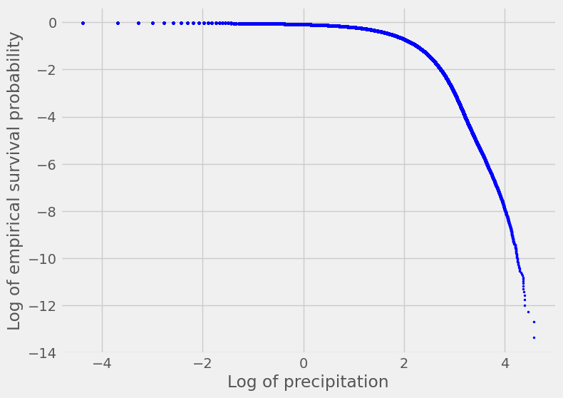
Refer to caption
(a) Histogram of precipitation
Refer to caption
(b) Log-log plot of precipitation
Figure 3: Histogram and log-log plot of precipitation. The blue and red horizontal lines represent the sample mean and the 99%99\% quantile of precipitation.
Refer to caption
Figure 4: Subfigures (a)–(d) show the differences in the predicted ES of precipitation between El Niño and non-El Niño conditions across the four seasons, while subfigures (e)–(h) show the corresponding differences in the predicted mean precipitation. In the plots, red indicates increased precipitation during El Niño, and blue represents decreased precipitation.

We fit the proposed robust ES regression at the upper-tail level α=0.99\alpha=0.99, with the robustification parameter selected according to the tuning procedure described in Section 2.4. The primary covariate of interest is the ENSO (Niño-3.43.4 index), while additional control variables include YEAR, SEASON, and the spatial coordinates LAT (latitude) and LON (longitude) of each grid point within the continental United States. To construct the Niño-3.43.4 index, we compute monthly averages of sea surface temperature in the Niño-3.43.4 region, subtract the corresponding annual mean, and normalize the resulting series. As noted in Remark 3, estimating the conditional upper-tail average at level α\alpha is equivalent to applying the proposed DRES method at level 1−α1-\alpha after negating the response variable. The conditional quantile function at level α\alpha is estimated using the DQR estimator defined in (2.2). For implementation, we employ fully connected ReLU neural networks with depth L=4L=4 and width N=512N=512, implemented in PyTorch. The learning rate is set to 10−310^{-3}, with a batch size of 1,024 and a total of 500 epochs. Following the procedure in Section 4.1, we reserve a validation set of size nvalid=⌈n/5⌉n_{\mathrm{valid}}=\lceil n/5\rceil to select the best-performing model across the 500 training epochs.

To assess the impact of El Niño on the upper tail of precipitation, we first compute the predicted conditional ES of precipitation at level α=0.99\alpha=0.99 for each grid location, setting the Niño-3.4 index set to 1.01.0 (representing El Niño conditions) and 0 (representing neutral conditions). To mitigate variability arising from random splits of the training and validation sets, the model-fitting procedure is repeated 10 times. In addition, to reduce the influence of year-specific fluctuations, we average the predicted values over the period 1991-2010. Subfigures (a)–(d) of Figure 4 display the differences in predicted ES between El Niño and non-El Niño conditions for each season. The remaining subfigures present the corresponding differences in predicted mean precipitation, obtained using the same procedure–10 repetitions and 20-year averaging–based on deep neural network mean regression.

Refer to caption
(a) Mean
Refer to caption
(b) 1% upper ES
Figure 5: Variable permutation importance for conditional mean and ES regressions.

Our results reveal that the influence of El Niño varies substantially across both space and season. In particular, during winter and spring, both regression approaches predict drier conditions in the northern United States and wetter conditions in the southern regions under El Niño episodes, consistent with the well-documented north-south seesaw pattern in precipitation reported in the climate science literature (DCDM1998). Notably, in winter, the spatial teleconnections are more pronounced when examining the upper-tail average than the mean. The ES regression uncovers a stronger linkage between ENSO and precipitation in southern California and along the Gulf Coast, consistent with earlier studies (KS2007), whereas the mean regression indicates only a weak association in these areas.

Additionally, we employ Variable Permutation Importance (VPI) (B2001) to quantify the contribution of individual features to predicting both mean and upper-tail average precipitation. The VPI for a given feature is computed by randomly permuting its sample values while holding all other variables fixed and then measuring the resulting relative increase in prediction loss. For mean regression, model performance is evaluated using the mean squared error (MSE) computed with respect to the original outcome YY. In contrast, for ES regression, the MSE is calculated with respect to the estimated surrogate response variable defined in (2.3). Figure 5 displays boxplots of the VPI values for the mean (left) and the 1% upper ES (right), showing the relative increases in losses, ordered by their average magnitudes.

The feature LON (longitude) exhibits the highest VPI for both mean and upper-tail ES regression. This likely reflects the influence of longitudinal geographic features–most notably, the Rocky Mountains and the Appalachian Mountains–which generate strong orographic effects on precipitation (H2012). Moreover, longitudinal variation in distance from the oceans also plays a key role in shaping precipitation patterns (C2019). Interestingly, the importance of LAT (latitude) increases when focusing on the upper percentiles of precipitation. Because latitude is strongly linked to temperature, which governs atmospheric circulation and air mass characteristics, it substantially contributes to regional precipitation variability across the United States. Overall, these findings provide a more nuanced understanding of how multiple factors, including El Ni no events, jointly influence the upper tails of U.S. precipitation distributions.

Acknowledgments and Disclosure of Funding

The authors would like to thank the Action Editor, Professor Jie Peng, and the two anonymous reviewers for their insightful comments and constructive suggestions that helped improve this work. The research of Kean Ming Tan was supported by the NSF grants DMS-2113346 and DMS-2238428. The research of Judy Wang was partially supported by the NSF grant DMS-2426174. Wen-Xin Zhou, the corresponding author, acknowledges travel support from the Australian Research Council Discovery Project Grant DP230100147.

Appendix A Proofs of Main Theorems

A.1 Supporting technical lemmas

We first introduce some basic notations that will be used throughout. Recall that quantile regression residuals are defined as ϵi=Yi−f0​(Xi)\epsilon_{i}=Y_{i}-f_{0}(X_{i}) for 1≤i≤n1\leq i\leq n and ϵ=Y−f0​(X)\epsilon=Y-f_{0}(X). For any f:[0,1]d→ℝf:[0,1]^{d}\to\mathbb{R}, we define

Z​(f)​(X,ϵ)={Y−f​(X)}​𝟙​{Y≤f​(X)}+α​f​(X),\displaystyle Z(f)(X,\epsilon)=\{Y-f(X)\}\mathbbm{1}\{Y\leq f(X)\}+\alpha f(X), (A.1)

and denote Zi​(f):=Z​(f)​(Xi,ϵi)Z_{i}(f):=Z(f)(X_{i},\epsilon_{i}) for 1≤i≤n1\leq i\leq n. Furthermore, we write

ωi=Z​(f0)​(Xi,ϵi)−α​g0​(Xi).\displaystyle\omega_{i}=Z(f_{0})(X_{i},\epsilon_{i})-\alpha g_{0}(X_{i}). (A.2)

Then, for any τ>0\tau>0, we can express the empirical joint Huber loss (2.4) as

ℛ^τ​(f,g)=1n​∑i=1nℓτ​(Zi​(f)−α​g​(Xi))\displaystyle\widehat{\mathcal{R}}_{\tau}(f,g)=\frac{1}{n}\sum_{i=1}^{n}\ell_{\tau}(Z_{i}(f)-\alpha g(X_{i}))

for real-valued functions f,gf,g on [0,1]d[0,1]^{d}. Also, note that

ωi=ϵi​𝟙​(ϵi≤0)+α​f0​(Xi)−α​g0​(Xi)=ϵi,−−𝔼​(ϵi,−|Xi),\displaystyle\omega_{i}=\epsilon_{i}\mathbbm{1}(\epsilon_{i}\leq 0)+\alpha f_{0}(X_{i})-\alpha g_{0}(X_{i})=\epsilon_{i,-}-\mathbb{E}(\epsilon_{i,-}|X_{i}),

where ϵi,−=ϵi​𝟙​(ϵi≤0)\epsilon_{i,-}=\epsilon_{i}\mathbbm{1}(\epsilon_{i}\leq 0). Throughout the proof, we assume that max⁡(‖f0‖∞,‖g0‖∞)≤M0\max(\|f_{0}\|_{\infty},\|g_{0}\|_{\infty})\leq M_{0}. For ease of notations, we write ∑i=1n(Wi−𝔼​Wi)=∑i=1n(1−𝔼)​Wi\sum_{i=1}^{n}(W_{i}-\mathbb{E}W_{i})=\sum_{i=1}^{n}(1-\mathbb{E})W_{i} for any sequence of random variables {Wi}i=1n\{W_{i}\}_{i=1}^{n}.

To establish a convergence rate for the deep quantile regression estimator, we require lower and upper bounds on the excess quantile risk. Recalling the definition of 𝒬^α​(f)\widehat{\mathcal{Q}}_{\alpha}(f) in (2.2), we define the population check loss function as

𝒬α​(f)=𝔼​𝒬^α​(f)=𝔼​ρα​(Yi−f​(Xi))\displaystyle\mathcal{Q}_{\alpha}(f)=\mathbb{E}\widehat{\mathcal{Q}}_{\alpha}(f)=\mathbb{E}\rho_{\alpha}(Y_{i}-f(X_{i}))

for any f:[0,1]d→ℝf:[0,1]^{d}\to\mathbb{R}.

Lemma 21.

Assume Condition 3.1 holds. For any function f:[0,1]d→[−M0,M0]f:[0,1]^{d}\to[-M_{0},M_{0}], the population check loss function satisfies

c14​‖f−f0‖22≤𝒬α​(f)−𝒬α​(f0)≤c15​‖f−f0‖22,\displaystyle c_{14}\|f-f_{0}\|_{2}^{2}\leq\mathcal{Q}_{\alpha}(f)-\mathcal{Q}_{\alpha}(f_{0})\leq c_{15}\|f-f_{0}\|_{2}^{2},

where c14=min⁡{p¯/(8​M0),p¯2/(32​M0​l0)}c_{14}=\min\{\underline{p}/(8M_{0}),\underline{p}^{2}/(32M_{0}l_{0})\} and c15=p¯/2c_{15}=\bar{p}/2.

Next, we write ℱn=ℱDNN​(d,Lq,Nq,M0)\mathcal{F}_{n}=\mathcal{F}_{{\rm DNN}}(d,L_{q},N_{q},M_{0}), and for any δ>0\delta>0,

ℱn​(δ)={f∈ℱn:‖f−f0‖2≤δ}.\displaystyle\mathcal{F}_{n}(\delta)=\{f\in\mathcal{F}_{n}:\|f-f_{0}\|_{2}\leq\delta\}.

The next lemma characterizes the tail probabilities of the empirical quantile process. Recall that δs=Lq​Nq​{d​log⁡(d​Lq​Nq)​log⁡n}/n\delta_{{\rm s}}=L_{q}N_{q}\sqrt{\{d\log(dL_{q}N_{q})\log n\}/n}.

Lemma 22.

There exists a universal constant c16>0c_{16}>0 such that for any δ≥δs\delta\geq\delta_{{\rm s}} and 0≤x≤n​δ20\leq x\leq n\delta^{2},

ℙ​[supf∈ℱn​(δ)|1n​∑i=1n(1−𝔼)​{ρα​(Yi−f​(Xi))−ρα​(Yi−f0​(Xi))}|≥c16⋅δ​(δs+xn)]≤e−x.\displaystyle\mathbb{P}\Bigg[\sup_{f\in\mathcal{F}_{n}(\delta)}\bigg|\frac{1}{n}\sum_{i=1}^{n}(1-\mathbb{E})\big\{\rho_{\alpha}(Y_{i}-f(X_{i}))-\rho_{\alpha}(Y_{i}-f_{0}(X_{i}))\big\}\bigg|\geq c_{16}\cdot\delta\bigg(\delta_{{\rm s}}+\sqrt{\frac{x}{n}}\bigg)\Bigg]\leq e^{-x}.

For the convergence rate for the DRES, recall that ℛτ​(⋅,⋅)\mathcal{R}_{\tau}(\cdot,\cdot) represents the population joint loss function, which is the expectation of the empirical joint Huber loss function,

ℛτ​(f,g)=𝔼​ℛ^τ​(f,g)=𝔼​ℓτ​(Zi​(f)−α​g​(Xi))\displaystyle\mathcal{R}_{\tau}(f,g)=\mathbb{E}\widehat{\mathcal{R}}_{\tau}(f,g)=\mathbb{E}\ell_{\tau}(Z_{i}(f)-\alpha g(X_{i}))

for any fixed functions ff and gg. The following two lemmas establish both lower and upper bounds for the excess Huber risk under heavy-tailed noises and light-tailed noises, respectively.

Lemma 23.

Assume Condition 2.1 with p>1p>1 and Condition 3.1 (i) hold and let τ≥c6=2​max⁡{4​M0,(2​νp)1/p}\tau\geq c_{6}=2\max\{4M_{0},(2\nu_{p})^{1/p}\}. Then, for any f,g:[0,1]d→[−M0,M0]f,g:[0,1]^{d}\to[-M_{0},M_{0}], we have

ℛτ​(f,g)−ℛτ​(f,g0)≥α24​‖g−g0‖22−α​‖g−g0‖2​{p¯2‖f−f0∥42+νp(τ/2)p−1},\displaystyle\mathcal{R}_{\tau}(f,g)-\mathcal{R}_{\tau}(f,g_{0})\geq\frac{\alpha^{2}}{4}\|g-g_{0}\|_{2}^{2}-\alpha\|g-g_{0}\|_{2}\bigg\{\frac{\bar{p}}{2}\|f-f_{0}\|_{4}^{2}+\frac{\nu_{p}}{(\tau/2)^{p-1}}\bigg\},

and

ℛτ​(f,g)−ℛτ​(f,g0)≤α22​‖g−g0‖22+α​‖g−g0‖2​{p¯2‖f−f0∥42+νp(τ/2)p−1}.\displaystyle\mathcal{R}_{\tau}(f,g)-\mathcal{R}_{\tau}(f,g_{0})\leq\frac{\alpha^{2}}{2}\|g-g_{0}\|_{2}^{2}+\alpha\|g-g_{0}\|_{2}\bigg\{\frac{\bar{p}}{2}\|f-f_{0}\|_{4}^{2}+\frac{\nu_{p}}{(\tau/2)^{p-1}}\bigg\}.
Lemma 24.

Assume Condition 3.2 holds for some σ0>0\sigma_{0}>0 and let

τ≥c9=2​max⁡{4​M0,σ0​(log⁡4)1/2}.\displaystyle\tau\geq c_{9}=2\max\{4M_{0},\sigma_{0}(\log 4)^{1/2}\}.

For any functions f,g:[0,1]d→[−M0,M0]f,g:[0,1]^{d}\to[-M_{0},M_{0}], we have

ℛτ​(f,g)−ℛτ​(f,g0)≥α24​‖g−g0‖22−α​‖g−g0‖2​(p¯2​‖f−f0‖42+c17​e−τ2/(2​σ02))\displaystyle\mathcal{R}_{\tau}(f,g)-\mathcal{R}_{\tau}(f,g_{0})\geq\frac{\alpha^{2}}{4}\|g-g_{0}\|_{2}^{2}-\alpha\|g-g_{0}\|_{2}\bigg(\frac{\bar{p}}{2}\|f-f_{0}\|_{4}^{2}+c_{17}e^{-\tau^{2}/(2\sigma_{0}^{2})}\bigg)

and

ℛτ​(f,g)−ℛτ​(f,g0)≤α22​‖g−g0‖22+α​‖g−g0‖2​(p¯2​‖f−f0‖42+c17​e−τ2/(2​σ02)),\displaystyle\mathcal{R}_{\tau}(f,g)-\mathcal{R}_{\tau}(f,g_{0})\leq\frac{\alpha^{2}}{2}\|g-g_{0}\|_{2}^{2}+\alpha\|g-g_{0}\|_{2}\bigg(\frac{\bar{p}}{2}\|f-f_{0}\|_{4}^{2}+c_{17}e^{-\tau^{2}/(2\sigma_{0}^{2})}\bigg),

where c17=4​M0+2​σ0c_{17}=4M_{0}+2\sigma_{0}.

For the truncated neural network function class 𝒢n=ℱDNN​(d,Le,Ne,M0)\mathcal{G}_{n}=\mathcal{F}_{{\rm DNN}}(d,L_{e},N_{e},M_{0}), define

𝒢n​(η)={g∈𝒢n:‖g−g0‖2≤η},η>0.\displaystyle\mathcal{G}_{n}(\eta)=\{g\in\mathcal{G}_{n}:\|g-g_{0}\|_{2}\leq\eta\},\ \ \eta>0.

Moreover, for any function pair (f,g)(f,g), we denote the difference of Huber losses as

hf,g​(X,ϵ)=ℓτ​(Z​(f)​(X,ϵ)−α​g​(X))−ℓτ​(Z​(f)​(X,ϵ)−α​g0​(X)).\displaystyle h_{f,g}(X,\epsilon)=\ell_{\tau}(Z(f)(X,\epsilon)-\alpha g(X))-\ell_{\tau}(Z(f)(X,\epsilon)-\alpha g_{0}(X)). (A.3)

In order to obtain the convergence rate of the ES estimator g^n\widehat{g}_{n} given a DQR estimate f^n∈ℱn\widehat{f}_{n}\in\mathcal{F}_{n}, it is necessary to derive concentration inequalities for the supremum of local empirical processes that are of the form

supf∈ℱnsupg∈𝒢n​(η)|1n​∑i=1n{hf,g​(Xi,ϵi)−𝔼​hf,g​(Xi,ϵi)}|\displaystyle\sup_{f\in\mathcal{F}_{n}}\sup_{g\in\mathcal{G}_{n}(\eta)}\bigg|\frac{1}{n}\sum_{i=1}^{n}\big\{h_{f,g}(X_{i},\epsilon_{i})-\mathbb{E}h_{f,g}(X_{i},\epsilon_{i})\big\}\bigg|

for some η>0\eta>0. To this end, by the fundamental theorem of calculus and the triangle inequality, the supremum is upper bounded by a sum of three suprema, namely,

supf∈ℱnsupg∈𝒢n​(η)|1n​∑i=1n(1−𝔼)​hf,g​(Xi,ϵi)|\displaystyle\sup_{f\in\mathcal{F}_{n}}\sup_{g\in\mathcal{G}_{n}(\eta)}\bigg|\frac{1}{n}\sum_{i=1}^{n}(1-\mathbb{E})h_{f,g}(X_{i},\epsilon_{i})\bigg|
=supf∈ℱnsupg∈𝒢n​(η)|1n​∑i=1n(1−𝔼)​{∫0α​Δg​(Xi)ψτ​(ωi+Zi​(f)−Zi​(f0)+t)​dt}|\displaystyle=\sup_{f\in\mathcal{F}_{n}}\sup_{g\in\mathcal{G}_{n}(\eta)}\bigg|\frac{1}{n}\sum_{i=1}^{n}(1-\mathbb{E})\bigg\{\int_{0}^{\alpha\Delta_{g}(X_{i})}\psi_{\tau}(\omega_{i}+Z_{i}(f)-Z_{i}(f_{0})+t){\rm d}t\bigg\}\bigg|
≤supg∈𝒢n​(η)|1n​∑i=1n(1−𝔼)​{∫0α​Δg​(Xi)ψτ​(ωi)​dt}|\displaystyle\leq\sup_{g\in\mathcal{G}_{n}(\eta)}\bigg|\frac{1}{n}\sum_{i=1}^{n}(1-\mathbb{E})\bigg\{\int_{0}^{\alpha\Delta_{g}(X_{i})}\psi_{\tau}(\omega_{i}){\rm d}t\bigg\}\bigg| (A.4)
+supg∈𝒢n​(η)|1n​∑i=1n(1−𝔼)​[∫0α​Δg​(Xi){ψτ​(ωi+t)−ψτ​(ωi)}​dt]|\displaystyle\penalty 10000\ \penalty 10000\ \penalty 10000\ \penalty 10000\ +\sup_{g\in\mathcal{G}_{n}(\eta)}\bigg|\frac{1}{n}\sum_{i=1}^{n}(1-\mathbb{E})\bigg[\int_{0}^{\alpha\Delta_{g}(X_{i})}\{\psi_{\tau}(\omega_{i}+t)-\psi_{\tau}(\omega_{i})\}{\rm d}t\bigg]\bigg|
+supf∈ℱnsupg∈𝒢n​(η)|1n​∑i=1n(1−𝔼)​[∫0α​Δg​(Xi){ψτ​(ωi+Zi​(f)−Zi​(f0)+t)−ψτ​(ωi+t)}​dt]|,\displaystyle\penalty 10000\ \penalty 10000\ \penalty 10000\ \penalty 10000\ +\sup_{f\in\mathcal{F}_{n}}\sup_{g\in\mathcal{G}_{n}(\eta)}\bigg|\frac{1}{n}\sum_{i=1}^{n}(1-\mathbb{E})\bigg[\int_{0}^{\alpha\Delta_{g}(X_{i})}\big\{\psi_{\tau}(\omega_{i}+Z_{i}(f)-Z_{i}(f_{0})+t)-\psi_{\tau}(\omega_{i}+t)\big\}{\rm d}t\bigg]\bigg|,

where Δg​(X)=g0​(X)−g​(X)\Delta_{g}(X)=g_{0}(X)-g(X) and ψτ=ℓτ′\psi_{\tau}=\ell_{\tau}^{\prime}. The following three lemmas give concentration inequalities for the above three suprema. Recall that

Vn,τ,νp=Le​Ne​d​log⁡(d​Le​Ne)​log⁡(n2​τ​νp−1/p)n​ and ​Vn=Le​Ne​d​log⁡(d​Le​Ne)​log⁡nn.\displaystyle V_{n,\tau,\nu_{p}}=L_{e}N_{e}\sqrt{\frac{d\log(dL_{e}N_{e})\log(n^{2}\tau\nu_{p}^{-1/p})}{n}}\penalty 10000\ \mbox{ and }\penalty 10000\ V_{n}=L_{e}N_{e}\sqrt{\frac{d\log(dL_{e}N_{e})\log n}{n}}.
Lemma 25.

Assume 𝔼​(|ωi|p|Xi)≤νp<∞\mathbb{E}(|\omega_{i}|^{p}|X_{i})\leq\nu_{p}<\infty almost surely (over XiX_{i}) for p>1p>1. Then, there exists a universal constant c18>0c_{18}>0 such that, for any η≥max⁡(τ​Vn,τ,νp,1/n),0≤x≤n​η2/τ\eta\geq\max(\sqrt{\tau}V_{n,\tau,\nu_{p}},1/n),0\leq x\leq n\eta^{2}/\tau and τ≥νp1/p\tau\geq\nu_{p}^{1/p},

ℙ{supg∈𝒢n​(η)|1n∑i=1n(1−𝔼)mg(Xi,ϵi)|≥c18⋅\displaystyle\mathbb{P}\Bigg\{\sup_{g\in\mathcal{G}_{n}(\eta)}\bigg|\frac{1}{n}\sum_{i=1}^{n}(1-\mathbb{E})m_{g}(X_{i},\epsilon_{i})\bigg|\geq c_{18}\cdot η​{τmax⁡(1−p/2,0)​νpmin⁡(1/2,1/p)+τ}\displaystyle\eta\{\tau^{\max(1-p/2,0)}\nu_{p}^{\min(1/2,1/p)}+\sqrt{\tau}\}
⋅(Vn,τ,νp+xn)}≤e−x.\displaystyle\penalty 10000\ \penalty 10000\ \penalty 10000\ \penalty 10000\ \penalty 10000\ \cdot\bigg(V_{n,\tau,\nu_{p}}+\sqrt{\frac{x}{n}}\bigg)\Bigg\}\leq e^{-x}.
Lemma 26.

There exists a universal constant c19>0c_{19}>0 such that for any τ>0,η≥Vn\tau>0,\eta\geq V_{n} and 0≤x≤n​η20\leq x\leq n\eta^{2},

ℙ​[supg∈𝒢n​(η)|1n​∑i=1n(1−𝔼)​[∫0α​Δg​(Xi){ψτ​(ωi+t)−ψτ​(ωi)}​dt]|≥c19⋅α2​η​(Vn+xn)]\displaystyle\mathbb{P}\Bigg[\sup_{g\in\mathcal{G}_{n}(\eta)}\bigg|\frac{1}{n}\sum_{i=1}^{n}(1-\mathbb{E})\bigg[\int_{0}^{\alpha\Delta_{g}(X_{i})}\{\psi_{\tau}(\omega_{i}+t)-\psi_{\tau}(\omega_{i})\}{\rm d}t\bigg]\bigg|\geq c_{19}\cdot\alpha^{2}\eta\bigg(V_{n}+\sqrt{\frac{x}{n}}\bigg)\Bigg]
≤e−x.\displaystyle\leq e^{-x}.
Lemma 27.

There exists a universal constant c20>0c_{20}>0 such that for any τ>0,η≥(δs+Vn)\tau>0,\eta\geq(\delta_{{\rm s}}+V_{n}) and 0≤x≤n​η20\leq x\leq n\eta^{2},

ℙ{supf∈ℱnsupg∈𝒢n​(η)|1n∑i=1n(1−𝔼)[∫0α​Δg​(Xi){ψτ(ωi+Zi(f)−Zi(f0)+t)−ψτ(ωi+t)}dt]|\displaystyle\mathbb{P}\Bigg\{\sup_{f\in\mathcal{F}_{n}}\sup_{g\in\mathcal{G}_{n}(\eta)}\bigg|\frac{1}{n}\sum_{i=1}^{n}(1-\mathbb{E})\bigg[\int_{0}^{\alpha\Delta_{g}(X_{i})}\big\{\psi_{\tau}(\omega_{i}+Z_{i}(f)-Z_{i}(f_{0})+t)-\psi_{\tau}(\omega_{i}+t)\big\}{\rm d}t\bigg]\bigg|
≥c20⋅αη(δs+Vn+xn)}≤e−x.\displaystyle\penalty 10000\ \penalty 10000\ \penalty 10000\ \penalty 10000\ \penalty 10000\ \penalty 10000\ \penalty 10000\ \penalty 10000\ \penalty 10000\ \penalty 10000\ \penalty 10000\ \penalty 10000\ \penalty 10000\ \penalty 10000\ \penalty 10000\ \penalty 10000\ \penalty 10000\ \penalty 10000\ \penalty 10000\ \penalty 10000\ \penalty 10000\ \penalty 10000\ \penalty 10000\ \penalty 10000\ \penalty 10000\ \penalty 10000\ \penalty 10000\ \penalty 10000\ \penalty 10000\ \penalty 10000\ \penalty 10000\ \penalty 10000\ \penalty 10000\ \penalty 10000\ \penalty 10000\ \penalty 10000\ \penalty 10000\ \penalty 10000\ \penalty 10000\ \penalty 10000\ \penalty 10000\ \penalty 10000\ \penalty 10000\ \penalty 10000\ \penalty 10000\ \penalty 10000\ \penalty 10000\ \penalty 10000\ \penalty 10000\ \penalty 10000\ \penalty 10000\ \penalty 10000\ \penalty 10000\ \penalty 10000\ \penalty 10000\ \penalty 10000\ \penalty 10000\ \penalty 10000\ \penalty 10000\ \penalty 10000\ \penalty 10000\ \penalty 10000\ \penalty 10000\ \penalty 10000\ \geq c_{20}\cdot\alpha\eta\bigg(\delta_{{\rm s}}+V_{n}+\sqrt{\frac{x}{n}}\bigg)\Bigg\}\leq e^{-x}.

Assuming that the random variables ωi\omega_{i} defined in (A.2) are sub-Gaussian, we can derive a more refined tail inequality for the supremum of local empirical processes.

Lemma 28.

Assume that ωi\omega_{i} satisfies

𝔼​(eωi2/σ02|Xi)≤2 almost surely (over Xi)\displaystyle\mathbb{E}\big(e^{\omega_{i}^{2}/\sigma_{0}^{2}}|X_{i}\big)\leq 2\penalty 10000\ \penalty 10000\ \mbox{ almost surely (over $X_{i}$)} (A.5)

for some σ0>0\sigma_{0}>0. Then, there exists a universal constant c21>0c_{21}>0 such that for any η≥Vn\eta\geq V_{n} and 0≤x≤n​η20\leq x\leq n\eta^{2}, the following bound

supg∈𝒢n​(η)|1n​∑i=1n(1−𝔼)​{∫0α​Δg​(Xi)ψτ​(ωi)​dt}|≤c21⋅α​σ0​η​{Vn+e−τ2/(2​σ02)+xn}\displaystyle\sup_{g\in\mathcal{G}_{n}(\eta)}\bigg|\frac{1}{n}\sum_{i=1}^{n}(1-\mathbb{E})\bigg\{\int_{0}^{\alpha\Delta_{g}(X_{i})}\psi_{\tau}(\omega_{i}){\rm d}t\bigg\}\bigg|\leq c_{21}\cdot\alpha\sigma_{0}\eta\bigg\{V_{n}+e^{-\tau^{2}/(2\sigma_{0}^{2})}+\sqrt{\frac{x}{n}}\bigg\}

holds with probability at least 1−3​e−x1-3e^{-x}.

A.2 Proof of Proposition 1

In the proof, we first construct a function g0,τg_{0,\tau} satisfying

g0,τ∈argming𝔼​{ℓτ​(Zi​(f0)−α​g​(Xi))}.\displaystyle g_{0,\tau}\in\mathop{\mathrm{argmin}}_{g}\mathbb{E}\{\ell_{\tau}(Z_{i}(f_{0})-\alpha g(X_{i}))\}. (A.6)

Then, we show that g0,τg_{0,\tau} satisfies the bound in Proposition 1. Finally, we show that g0,τg_{0,\tau} is the unique minimizer of (A.6) almost surely over XX.

To begin with, recall that Zi​(f0)=α​g0​(X)+ωiZ_{i}(f_{0})=\alpha g_{0}(X)+\omega_{i} with ωi=ϵi,−−𝔼​(ϵi,−|X)\omega_{i}=\epsilon_{i,-}-\mathbb{E}(\epsilon_{i,-}|X). For each x∈𝒳x\in\mathcal{X}, consider

mina∈ℝ𝔼{ℓτ(Zi(f0)−αa)|X=x}=𝔼{ℓτ(ωi+αg0(x)−αa)|X=x}=:Lx(a).\displaystyle\min_{a\in\mathbb{R}}\mathbb{E}\{\ell_{\tau}(Z_{i}(f_{0})-\alpha a)|X=x\}=\mathbb{E}\{\ell_{\tau}(\omega_{i}+\alpha g_{0}(x)-\alpha a)|X=x\}=:L_{x}(a).

Since (i) Lx​(a)L_{x}(a) is convex and (ii) Lx​(a)→∞L_{x}(a)\to\infty as a→±∞a\to\pm\infty, the set of minimizers is nonempty for each xx. Let Ψ​(x)\Psi(x) denote this set. By the Kuratowski–Ryll-Nardzewski measurable selection theorem (Theorem 6.9.3 in bogachev2007measure), there exists a measurable function g0,τg_{0,\tau} such that g0,τ​(x)∈Ψ​(x)g_{0,\tau}(x)\in\Psi(x) for all x∈𝒳x\in\mathcal{X}. For any measurable function gg (not necessarily bounded by M0M_{0}), we then have

𝔼​{ℓτ​(Zi​(f0)−α​g​(X))|X=x}≥𝔼​{ℓτ​(Zi​(f0)−α​g0,τ​(X))|X=x},\displaystyle\mathbb{E}\{\ell_{\tau}(Z_{i}(f_{0})-\alpha g(X))|X=x\}\geq\mathbb{E}\{\ell_{\tau}(Z_{i}(f_{0})-\alpha g_{0,\tau}(X))|X=x\}, (A.7)

which implies

𝔼​{ℓτ​(Zi​(f0)−α​g​(X))}≥𝔼​{ℓτ​(Zi​(f0)−α​g0,τ​(X))}.\displaystyle\mathbb{E}\{\ell_{\tau}(Z_{i}(f_{0})-\alpha g(X))\}\geq\mathbb{E}\{\ell_{\tau}(Z_{i}(f_{0})-\alpha g_{0,\tau}(X))\}. (A.8)

Hence, g0,τg_{0,\tau} is a minimizer.

To obtain a bound for g0,τg_{0,\tau}, we follow a similar argument as in the proof of Proposition 1 in sun2020adaptive. Specifically, define Δx=g0​(x)−g0,τ​(x)\Delta_{x}=g_{0}(x)-g_{0,\tau}(x) for each x∈𝒳x\in\mathcal{X}. For convenience, fix x∈𝒳x\in\mathcal{X} and denote g0,τ​(x)=aτ∗g_{0,\tau}(x)=a_{\tau}^{*} and g0​(x)=a∗g_{0}(x)=a^{*}. By the optimality of aτ∗a_{\tau}^{*} and the mean value theorem, we have Lx′​(aτ∗)=0L_{x}^{\prime}(a_{\tau}^{*})=0 and

Lx′′​(a~)​Δx2={Lx′​(a∗)−Lx′​(aτ∗)}​Δx=Lx′​(a∗)​Δx=−α​𝔼​{ψτ​(ω)|X=x}​Δx,\displaystyle L_{x}^{\prime\prime}(\widetilde{a})\Delta_{x}^{2}=\{L_{x}^{\prime}(a^{*})-L_{x}^{\prime}(a_{\tau}^{*})\}\Delta_{x}=L_{x}^{\prime}(a^{*})\Delta_{x}=-\alpha\mathbb{E}\{\psi_{\tau}(\omega)|X=x\}\Delta_{x}, (A.9)

where a~=λ​a∗+(1−λ)​aτ∗\widetilde{a}=\lambda a^{*}+(1-\lambda)a_{\tau}^{*} for some 0≤λ≤10\leq\lambda\leq 1. Since 𝔼​(ω|X=x)=0\mathbb{E}(\omega|X=x)=0 and

|𝔼{ω|X=x}−𝔼{ψτ(ω)|X=x}|=τ|ℙ(|ω|>τ|X=x)|≤𝔼​{|ω|p|X=x}τp−1,\displaystyle|\mathbb{E}\{\omega|X=x\}-\mathbb{E}\{\psi_{\tau}(\omega)|X=x\}|=\tau|\mathbb{P}(|\omega|>\tau|X=x)|\leq\frac{\mathbb{E}\{|\omega|^{p}|X=x\}}{\tau^{p-1}},

we have |𝔼​{ψτ​(ω)|X=x}|≤νp/τp−1|\mathbb{E}\{\psi_{\tau}(\omega)|X=x\}|\leq\nu_{p}/\tau^{p-1}. Now, letting ω~=Zi​(f0)−α​a~\widetilde{\omega}=Z_{i}(f_{0})-\alpha\widetilde{a}, we have

Lx′′​(a~)=α2​{1−ℙ​(|ω~|>τ|X=x)}.\displaystyle L_{x}^{\prime\prime}(\widetilde{a})=\alpha^{2}\{1-\mathbb{P}(|\widetilde{\omega}|>\tau|X=x)\}.

To bound ℙ​(|ω~|>τ|X=x)\mathbb{P}(|\widetilde{\omega}|>\tau|X=x), we remark that

ℙ​(|ω~|>τ|X=x)≤τ−1​𝔼​{|ω~|​𝟙​(|ω~|>τ)|X=x}.\displaystyle\mathbb{P}(|\widetilde{\omega}|>\tau|X=x)\leq\tau^{-1}\mathbb{E}\{|\widetilde{\omega}|\mathbbm{1}(|\widetilde{\omega}|>\tau)|X=x\}.

Now, since LxL_{x} is a convex function and minimized at aτ∗a_{\tau}^{*}, we have

Lx​(a~)≤λ​Lx​(a∗)+(1−λ)​Lx​(aτ∗)≤Lx​(a∗).\displaystyle L_{x}(\widetilde{a})\leq\lambda L_{x}(a^{*})+(1-\lambda)L_{x}(a_{\tau}^{*})\leq L_{x}(a^{*}). (A.10)

By definition, we have

Lx​(a∗)\displaystyle L_{x}(a^{*}) =𝔼​{|ω|22​𝟙​(|ω|≤τ)+(τ​|ω|−τ22)​𝟙​(|ω|>τ)|X=x}.\displaystyle=\mathbb{E}\bigg\{\frac{|\omega|^{2}}{2}\mathbbm{1}(|\omega|\leq\tau)+\bigg(\tau|\omega|-\frac{\tau^{2}}{2}\bigg)\mathbbm{1}(|\omega|>\tau)\bigg|X=x\bigg\}.

Therefore, it follows that

Lx​(a∗)\displaystyle L_{x}(a^{*}) ≤𝔼​{τmax⁡(2−p,0)​|ω|min⁡(p,2)2​𝟙​(|ω|≤τ)+τmax⁡(2−p,0)​|ω|min⁡(p,2)​𝟙​(|ω|>τ)|X=x}\displaystyle\leq\mathbb{E}\bigg\{\frac{\tau^{\max(2-p,0)}|\omega|^{\min(p,2)}}{2}\mathbbm{1}(|\omega|\leq\tau)+\tau^{\max(2-p,0)}|\omega|^{\min(p,2)}\mathbbm{1}(|\omega|>\tau)\bigg|X=x\bigg\}
≤μp​τmax⁡(2−p,0),\displaystyle\leq\mu_{p}\tau^{\max(2-p,0)},

where μp=νp\mu_{p}=\nu_{p} if 1<p<21<p<2 and μp=ν2\mu_{p}=\nu_{2} if p≥2p\geq 2. Thus, (A.10) implies Lx​(a~)≤μp​τmax⁡(2−p,0)L_{x}(\widetilde{a})\leq\mu_{p}\tau^{\max(2-p,0)}. Since we have

Lx​(a~)≥𝔼​{(τ​|ω~|−τ22)​𝟙​(|ω~|>τ)},\displaystyle L_{x}(\widetilde{a})\geq\mathbb{E}\bigg\{\bigg(\tau|\widetilde{\omega}|-\frac{\tau^{2}}{2}\bigg)\mathbbm{1}(|\widetilde{\omega}|>\tau)\bigg\},

it follows that

τ​𝔼​{|ω~|​𝟙​(|ω~|>τ)|X=x}\displaystyle\tau\mathbb{E}\{|\widetilde{\omega}|\mathbbm{1}(|\widetilde{\omega}|>\tau)|X=x\} ≤τ22​ℙ​(|ω~|>τ|X=x)+μp​τmax⁡(2−p,0)\displaystyle\leq\frac{\tau^{2}}{2}\mathbb{P}(|\widetilde{\omega}|>\tau|X=x)+\mu_{p}\tau^{\max(2-p,0)}
≤τ2​𝔼​{|ω~|​𝟙​(|ω~|>τ)|X=x}+μp​τmax⁡(2−p,0).\displaystyle\leq\frac{\tau}{2}\mathbb{E}\{|\widetilde{\omega}|\mathbbm{1}(|\widetilde{\omega}|>\tau)|X=x\}+\mu_{p}\tau^{\max(2-p,0)}.

Therefore, we have

𝔼​{|ω~|​𝟙​(|ω~|>τ)|X=x}≤2​μp​τmax⁡(1−p,−1),\displaystyle\mathbb{E}\{|\widetilde{\omega}|\mathbbm{1}(|\widetilde{\omega}|>\tau)|X=x\}\leq 2\mu_{p}\tau^{\max(1-p,-1)},

and

ℙ​(|ω~|>τ|X=x)≤2​μp​τmax⁡(−p,−2).\displaystyle\mathbb{P}(|\widetilde{\omega}|>\tau|X=x)\leq 2\mu_{p}\tau^{\max(-p,-2)}.

As a result, given that τ≥(4​μp)1/min⁡(p,2)\tau\geq(4\mu_{p})^{1/\min(p,2)}, we have Lx′′​(t~)≥α2/2L_{x}^{\prime\prime}(\widetilde{t})\geq\alpha^{2}/2, and combining this with (A.9) gives

α​|g0​(x)−g0,τ​(x)|≤2​|𝔼​{ψτ​(ω)|X=x}|≤2​νpτp−1.\displaystyle\alpha|g_{0}(x)-g_{0,\tau}(x)|\leq 2|\mathbb{E}\{\psi_{\tau}(\omega)|X=x\}|\leq\frac{2\nu_{p}}{\tau^{p-1}}.

Since the bound holds for any x∈𝒳x\in\mathcal{X}, so we obtain α​‖g0−g0,τ‖∞≤2​νp/τp−1\alpha\|g_{0}-g_{0,\tau}\|_{\infty}\leq 2\nu_{p}/\tau^{p-1}.

Finally, assume that g†g^{\dagger} is another minimizer of (A.6). Since any function gg satisfies (A.8), it follows that

0\displaystyle 0 =𝔼​{ℓτ​(Zi​(f0)−α​g†​(X))}−𝔼​{ℓτ​(Zi​(f0)−α​g0,τ​(X))}\displaystyle=\mathbb{E}\{\ell_{\tau}(Z_{i}(f_{0})-\alpha g^{\dagger}(X))\}-\mathbb{E}\{\ell_{\tau}(Z_{i}(f_{0})-\alpha g_{0,\tau}(X))\}
=𝔼​[𝔼​{ℓτ​(Zi​(f0)−α​g†​(X))|X}−𝔼​{ℓτ​(Zi​(f0)−α​g0,τ​(X))|X}]≥0.\displaystyle=\mathbb{E}[\mathbb{E}\{\ell_{\tau}(Z_{i}(f_{0})-\alpha g^{\dagger}(X))|X\}-\mathbb{E}\{\ell_{\tau}(Z_{i}(f_{0})-\alpha g_{0,\tau}(X))|X\}]\geq 0.

Therefore, combining with (A.7), we obtain

𝔼​{ℓτ​(Zi​(f0)−α​g†​(X))|X}−𝔼​{ℓτ​(Zi​(f0)−α​g0,τ​(X))|X}=0\displaystyle\mathbb{E}\{\ell_{\tau}(Z_{i}(f_{0})-\alpha g^{\dagger}(X))|X\}-\mathbb{E}\{\ell_{\tau}(Z_{i}(f_{0})-\alpha g_{0,\tau}(X))|X\}=0

almost surely over XX. Let x∈𝒳x\in\mathcal{X} be any element such that the above equation holds for X=xX=x. Denoting a†=g~​(x)a^{\dagger}=\widetilde{g}(x) and aτ∗=g0,τ​(x)a_{\tau}^{*}=g_{0,\tau}(x), we have Lx​(a†)=Lx​(aτ∗)L_{x}(a^{\dagger})=L_{x}(a_{\tau}^{*}) and a†a^{\dagger} is also a minimizer of LxL_{x}. Denoting Δx†=a†−aτ∗\Delta_{x}^{\dagger}=a^{\dagger}-a_{\tau}^{*}, applying the mean value theorem gives

Lx′′​(a~†)​Δx†2={Lx′​(a†)−Lx′​(aτ∗)}​Δx†=0,\displaystyle L_{x}^{\prime\prime}(\widetilde{a}^{\dagger})\Delta_{x}^{\dagger 2}=\{L_{x}^{\prime}(a^{\dagger})-L_{x}^{\prime}(a_{\tau}^{*})\}\Delta_{x}^{\dagger}=0,

where a~†\widetilde{a}^{\dagger} lies between a†a^{\dagger} and aτ∗a_{\tau}^{*}. Since both a†a^{\dagger} and aτ∗a_{\tau}^{*} are minimizers of LxL_{x}, it follows that Lx​(a~†)≤Lx​(a∗)L_{x}(\widetilde{a}^{\dagger})\leq L_{x}(a^{*}). By applying a similar argument as in the previous step, we further obtain that Lx​(a~†)′′≥1/2L_{x}(\widetilde{a}^{\dagger})^{\prime\prime}\geq 1/2 under the given condition on τ\tau. Hence, g†=g0,τg^{\dagger}=g_{0,\tau}, and the minimizer is unique almost surely with respect to the probability measure of XX. This completes the proof.

∎

A.3 Proof of Theorem 8

To begin with, let δ∗=c4​(δs+δa+u/n)\delta_{*}=c_{4}(\delta_{{\rm s}}+\delta_{{\rm a}}+\sqrt{u/n}) for given u≥1u\geq 1, where c4c_{4} is given by

c4=max{(8​c15/c14,2/c14,16c16/c14}≥1.\displaystyle c_{4}=\max\{(\sqrt{8c_{15}/c_{14}},\sqrt{2/c_{14}},16c_{16}/c_{14}\}\geq 1. (A.11)

Here, c14c_{14} and c15c_{15} are given in Lemma 21 and c16c_{16} is given in Lemma 22. We then define the donut-shaped sets for integers j=1,2,…j=1,2,\ldots as

𝒟n,j:=ℱn​(2j​δ∗)∖ℱn​(2j−1​δ∗)={f∈ℱn:2j−1​δ∗<‖f−f0‖2≤2j​δ∗},\displaystyle\mathcal{D}_{n,j}:=\mathcal{F}_{n}(2^{j}\delta_{*})\setminus\mathcal{F}_{n}(2^{j-1}\delta_{*})=\{f\in\mathcal{F}_{n}:2^{j-1}\delta_{*}<\|f-f_{0}\|_{2}\leq 2^{j}\delta_{*}\},

so that we can write

ℙ​{‖f^n−f0‖2≥δ∗}≤∑j=1∞ℙ​{f^n∈𝒟n,j}.\displaystyle\mathbb{P}\{\|\widehat{f}_{n}-f_{0}\|_{2}\geq\delta_{*}\}\leq\sum_{j=1}^{\infty}\mathbb{P}\{\widehat{f}_{n}\in\mathcal{D}_{n,j}\}. (A.12)

Therefore, it reduces to bounding each probability ℙ​{f^n∈𝒟n,j}\mathbb{P}\{\widehat{f}_{n}\in\mathcal{D}_{n,j}\} separately. Following Lemma 21, any f∈𝒟n,jf\in\mathcal{D}_{n,j} satisfies

c14​22​j−2​δ∗2≤c14​‖f−f0‖22≤𝒬α​(f)−𝒬α​(f0).\displaystyle c_{14}2^{2j-2}\delta_{*}^{2}\leq c_{14}\|f-f_{0}\|_{2}^{2}\leq\mathcal{Q}_{\alpha}(f)-\mathcal{Q}_{\alpha}(f_{0}). (A.13)

We next derive an upper bound of the right-hand side of (A.13). By the definition of δa\delta_{{\rm a}}, there exists fn∈ℱnf_{n}\in\mathcal{F}_{n} such that ‖fn−f0‖2≤2​δa\|f_{n}-f_{0}\|_{2}\leq 2\delta_{{\rm a}}. Now, if f^n∈𝒟n,j\widehat{f}_{n}\in\mathcal{D}_{n,j}, we have

𝒬α​(f^n)−𝒬α​(f0)\displaystyle\mathcal{Q}_{\alpha}(\widehat{f}_{n})-\mathcal{Q}_{\alpha}(f_{0})
=𝒬α​(f^n)−𝒬^α​(f^n)+𝒬^α​(f^n)−𝒬^α​(fn)+𝒬^α​(fn)−𝒬α​(fn)+𝒬α​(fn)−𝒬α​(f0)\displaystyle=\mathcal{Q}_{\alpha}(\widehat{f}_{n})-\widehat{\mathcal{Q}}_{\alpha}(\widehat{f}_{n})+\widehat{\mathcal{Q}}_{\alpha}(\widehat{f}_{n})-\widehat{\mathcal{Q}}_{\alpha}(f_{n})+\widehat{\mathcal{Q}}_{\alpha}(f_{n})-\mathcal{Q}_{\alpha}(f_{n})+\mathcal{Q}_{\alpha}(f_{n})-\mathcal{Q}_{\alpha}(f_{0})
≤𝒬α​(f^n)−𝒬^α​(f^n)+𝒬^α​(fn)−𝒬α​(fn)+𝒬α​(fn)−𝒬α​(f0),\displaystyle\leq\mathcal{Q}_{\alpha}(\widehat{f}_{n})-\widehat{\mathcal{Q}}_{\alpha}(\widehat{f}_{n})+\widehat{\mathcal{Q}}_{\alpha}(f_{n})-\mathcal{Q}_{\alpha}(f_{n})+\mathcal{Q}_{\alpha}(f_{n})-\mathcal{Q}_{\alpha}(f_{0}),

where the last line follows from the definition of f^n\widehat{f}_{n}. By Lemma 21, it follows that 𝒬α​(fn)−𝒬α​(f0)≤4​c15​δa2\mathcal{Q}_{\alpha}(f_{n})-\mathcal{Q}_{\alpha}(f_{0})\leq 4c_{15}\delta_{{\rm a}}^{2}. Denoting

Δn(f)=1n∑i=1n(1−𝔼){ρα(Yi−f(Xi)−ρα(Yi−f0(Xi)},\displaystyle\Delta_{n}(f)=\frac{1}{n}\sum_{i=1}^{n}(1-\mathbb{E})\big\{\rho_{\alpha}(Y_{i}-f(X_{i})-\rho_{\alpha}(Y_{i}-f_{0}(X_{i})\big\},

the earlier inequality is further bounded as

𝒬α​(f^n)−𝒬α​(f0)≤Δn​(fn)−Δn​(f^n)+4​c15​δa2.\displaystyle\mathcal{Q}_{\alpha}(\widehat{f}_{n})-\mathcal{Q}_{\alpha}(f_{0})\leq\Delta_{n}(f_{n})-\Delta_{n}(\widehat{f}_{n})+4c_{15}\delta_{{\rm a}}^{2}. (A.14)

Note that fn∈ℱn​(2j​δ∗)f_{n}\in\mathcal{F}_{n}(2^{j}\delta_{*}) for any j≥1j\geq 1 because 2​δa≤2j​δ∗2\delta_{{\rm a}}\leq 2^{j}\delta_{*} for any j≥1j\geq 1. Combining this with (A.14) and (A.13), we obtain upper bounds of the probability ℙ​{f^n∈𝒟n,j}\mathbb{P}\{\widehat{f}_{n}\in\mathcal{D}_{n,j}\} as

ℙ​{f^n∈𝒟n,j}\displaystyle\mathbb{P}\{\widehat{f}_{n}\in\mathcal{D}_{n,j}\} ≤ℙ​{∃f∈𝒟n,j​ such that ​Δn​(fn)−Δn​(f)≥c144​22​j​δ∗2−4​c15​δa2}\displaystyle\leq\mathbb{P}\bigg\{\exists f\in\mathcal{D}_{n,j}\mbox{ such that }\Delta_{n}(f_{n})-\Delta_{n}(f)\geq\frac{c_{14}}{4}2^{2j}\delta_{*}^{2}-4c_{15}\delta_{{\rm a}}^{2}\bigg\}
≤ℙ​{supf∈ℱn​(2j​δ∗)|Δn​(f)|≥c1416​22​j​δ∗2},\displaystyle\leq\mathbb{P}\Bigg\{\sup_{f\in\mathcal{F}_{n}(2^{j}\delta_{*})}|\Delta_{n}(f)|\geq\frac{c_{14}}{16}2^{2j}\delta_{*}^{2}\Bigg\}, (A.15)

where the last line follows from the choice of c4c_{4} in (A.11).

We next bound the probability ℙ​{supf∈ℱn​(2j​δ∗)|Δn​(f)|≥c14​22​j​δ∗2/16}\mathbb{P}\{\sup_{f\in\mathcal{F}_{n}(2^{j}\delta_{*})}|\Delta_{n}(f)|\geq c_{14}2^{2j}\delta_{*}^{2}/16\} via Lemma 22. To this end, we choose δ=2j​δ∗\delta=2^{j}\delta_{*} and x=22​j​ux=2^{2j}u. Since c4≥1c_{4}\geq 1, we have δ≥δs\delta\geq\delta_{{\rm s}} and 0≤x≤n​δ20\leq x\leq n\delta^{2}. Then, Lemma 22 yields

ℙ​{supf∈ℱn​(2j​δ∗)|Δn​(f)|≥c16c4​22​j​δ∗2}\displaystyle\mathbb{P}\Bigg\{\sup_{f\in\mathcal{F}_{n}(2^{j}\delta_{*})}|\Delta_{n}(f)|\geq\frac{c_{16}}{c_{4}}2^{2j}\delta_{*}^{2}\Bigg\}
=ℙ​[supf∈ℱn​(2j​δ∗)|1n​∑i=1n(1−𝔼)​{ρα​(Yi−f​(Xi))−ρα​(Yi−f0​(Xi))}|≥c16c4​22​j​δ∗2]\displaystyle=\mathbb{P}\Bigg[\sup_{f\in\mathcal{F}_{n}(2^{j}\delta_{*})}\bigg|\frac{1}{n}\sum_{i=1}^{n}(1-\mathbb{E})\big\{\rho_{\alpha}(Y_{i}-f(X_{i}))-\rho_{\alpha}(Y_{i}-f_{0}(X_{i}))\big\}\bigg|\geq\frac{c_{16}}{c_{4}}2^{2j}\delta_{*}^{2}\Bigg]
≤ℙ​[supf∈ℱn​(2j​δ∗)|1n​∑i=1n(1−𝔼)​{ρα​(Yi−f​(Xi))−ρα​(Yi−f0​(Xi))}|≥c16​δ​(δs+xn)]\displaystyle\leq\mathbb{P}\Bigg[\sup_{f\in\mathcal{F}_{n}(2^{j}\delta_{*})}\bigg|\frac{1}{n}\sum_{i=1}^{n}(1-\mathbb{E})\big\{\rho_{\alpha}(Y_{i}-f(X_{i}))-\rho_{\alpha}(Y_{i}-f_{0}(X_{i}))\big\}\bigg|\geq c_{16}\delta\bigg(\delta_{{\rm s}}+\sqrt{\frac{x}{n}}\bigg)\Bigg]
≤exp⁡(−x)=exp⁡(−22​j​u).\displaystyle\leq\exp(-x)=\exp(-2^{2j}u).

Since c4c_{4} satisfies c16/c4≤c14/16c_{16}/c_{4}\leq c_{14}/16, the above probability bound yields

ℙ​{supf∈ℱn​(2j​δ∗)|Δn​(f)|≥c1416​22​j​δ∗2}≤exp⁡(−22​j​u).\displaystyle\mathbb{P}\Bigg\{\sup_{f\in\mathcal{F}_{n}(2^{j}\delta_{*})}|\Delta_{n}(f)|\geq\frac{c_{14}}{16}2^{2j}\delta_{*}^{2}\Bigg\}\leq\exp(-2^{2j}u).

Combining this with (A.12) and (A.15) implies

ℙ​{‖f^n−f0‖2≥δ∗}\displaystyle\mathbb{P}\{\|\widehat{f}_{n}-f_{0}\|_{2}\geq\delta_{*}\} ≤∑j=1∞exp⁡(−22​j​u)≤∑j=1∞exp⁡(−j​u)≤(1−e−1)−1​e−u,\displaystyle\leq\sum_{j=1}^{\infty}\exp(-2^{2j}u)\leq\sum_{j=1}^{\infty}\exp(-ju)\leq(1-e^{-1})^{-1}e^{-u},

where the last inequality uses the fact that u≥1u\geq 1. This proves the claim. ∎

A.4 Proof of Theorem 13

Following a similar line to the proof of Theorem 13, we start with the peeling argument. To begin with, denote for any u≥1u\geq 1 fixed that

η∗=c7​{ηs+ηb+ηa+δs+δ42+(νp1/p+τ)​un},\displaystyle\eta_{*}=c_{7}\bigg\{\eta_{{\rm s}}+\eta_{{\rm b}}+\eta_{{\rm a}}+\delta_{{\rm s}}+\delta_{4}^{2}+(\nu_{p}^{1/p}+\sqrt{\tau})\sqrt{\frac{u}{n}}\bigg\},

where c7c_{7} is given by

c7=max⁡(24⋅7​p¯,28⋅24,192​c18,192​c19,192​c20)≥1.\displaystyle c_{7}=\max(\sqrt{24\cdot 7}\bar{p},\sqrt{28\cdot 24},192c_{18},192c_{19},192c_{20})\geq 1. (A.16)

Here, c18,c19c_{18},c_{19} and c20c_{20} are defined in Lemma 25, Lemma 26 and Lemma 27, respectively. For integers j=1,2,…,j=1,2,\dots, define donut-shaped sets

𝒟n,j:=𝒢n​(2j​η∗/α)∖𝒢n​(2j−1​η∗/α)={g∈𝒢n:2j−1​η∗​<α∥​g−g0∥2≤2j​η∗}.\displaystyle\mathcal{D}_{n,j}:=\mathcal{G}_{n}(2^{j}\eta_{*}/\alpha)\setminus\mathcal{G}_{n}(2^{j-1}\eta_{*}/\alpha)=\big\{g\in\mathcal{G}_{n}:2^{j-1}\eta_{*}<\alpha\|g-g_{0}\|_{2}\leq 2^{j}\eta_{*}\big\}.

Since we have

ℙ​(α​‖g^n−g0‖2≥η∗)≤∑j=1∞ℙ​(g^n∈𝒟n,j),\displaystyle\mathbb{P}\big(\alpha\|\widehat{g}_{n}-g_{0}\|_{2}\geq\eta_{*}\big)\leq\sum_{j=1}^{\infty}\mathbb{P}\big(\widehat{g}_{n}\in\mathcal{D}_{n,j}\big), (A.17)

it suffices to bound each probability on the right-hand side of the above inequality. Recall the local function class ℱ0​(δ)={f∈ℱn:‖f−f0‖4≤δ}\mathcal{F}_{0}(\delta)=\{f\in\mathcal{F}_{n}:\|f-f_{0}\|_{4}\leq\delta\} for any δ>0\delta>0. Conditioning on the event {f^n∈ℱ0​(δ4)}\{\widehat{f}_{n}\in\mathcal{F}_{0}(\delta_{4})\}, Lemma 23 implies that if g^n∈𝒟n,j\widehat{g}_{n}\in\mathcal{D}_{n,j}, we have

22​j−24​η∗2\displaystyle\frac{2^{2j-2}}{4}\eta_{*}^{2} ≤ℛτ​(f^n,g^n)−ℛτ​(f^n,g0)+2j​η∗​(p¯2​δ42+ηb)\displaystyle\leq\mathcal{R}_{\tau}(\widehat{f}_{n},\widehat{g}_{n})-\mathcal{R}_{\tau}(\widehat{f}_{n},g_{0})+2^{j}\eta_{*}\bigg(\frac{\bar{p}}{2}\delta_{4}^{2}+\eta_{{\rm b}}\bigg)
≤ℛτ​(f^n,g^n)−ℛτ​(f^n,g0)+6​p¯2​δ44+24​ηb2+22​j48​η∗2,\displaystyle\leq\mathcal{R}_{\tau}(\widehat{f}_{n},\widehat{g}_{n})-\mathcal{R}_{\tau}(\widehat{f}_{n},g_{0})+6\bar{p}^{2}\delta_{4}^{4}+24\eta_{{\rm b}}^{2}+\frac{2^{2j}}{48}\eta_{*}^{2}, (A.18)

where the last inequality follows from the basic inequalities a​b≤12​a2+b2/48ab\leq 12a^{2}+b^{2}/48 and (a+b)2≤2​(a2+b2)(a+b)^{2}\leq 2(a^{2}+b^{2}) for any a,b∈ℝa,b\in\mathbb{R}.

We will now establish an upper bound for ℛτ​(f^n,g^n)−ℛτ​(f^n,g0)\mathcal{R}_{\tau}(\widehat{f}_{n},\widehat{g}_{n})-\mathcal{R}_{\tau}(\widehat{f}_{n},g_{0}), which appears on the right-hand side of inequality (A.18). The definition of ηa\eta_{{\rm a}} in (3.6) allows us to choose gn∈𝒢ng_{n}\in\mathcal{G}_{n} such that ‖gn−g0‖2≤2​ηa\|g_{n}-g_{0}\|_{2}\leq 2\eta_{{\rm a}}. When we condition on the event {f^n∈ℱ0​(δ4)}\{\widehat{f}_{n}\in\mathcal{F}_{0}(\delta_{4})\}, g^n\widehat{g}_{n} satisfies that

ℛτ​(f^n,g^n)−ℛτ​(f^n,g0)\displaystyle\mathcal{R}_{\tau}(\widehat{f}_{n},\widehat{g}_{n})-\mathcal{R}_{\tau}(\widehat{f}_{n},g_{0})
≤ℛτ​(f^n,g^n)−ℛ^τ​(f^n,g^n)+ℛ^τ​(f^n,gn)−ℛτ​(f^n,gn)+ℛτ​(f^n,gn)−ℛτ​(f^n,g0).\displaystyle\leq\mathcal{R}_{\tau}(\widehat{f}_{n},\widehat{g}_{n})-\widehat{\mathcal{R}}_{\tau}(\widehat{f}_{n},\widehat{g}_{n})+\widehat{\mathcal{R}}_{\tau}(\widehat{f}_{n},g_{n})-\mathcal{R}_{\tau}(\widehat{f}_{n},g_{n})+\mathcal{R}_{\tau}(\widehat{f}_{n},g_{n})-\mathcal{R}_{\tau}(\widehat{f}_{n},g_{0}).

The upper bound in Lemma 23 with g=gng=g_{n} implies

ℛτ​(f^n,gn)−ℛτ​(f^n,g0)\displaystyle\mathcal{R}_{\tau}(\widehat{f}_{n},g_{n})-\mathcal{R}_{\tau}(\widehat{f}_{n},g_{0}) ≤2​α2​ηa2+α⋅ηa​(p¯2​δ42+ηb)\displaystyle\leq 2\alpha^{2}\eta_{{\rm a}}^{2}+\alpha\cdot\eta_{{\rm a}}\bigg(\frac{\bar{p}}{2}\delta_{4}^{2}+\eta_{{\rm b}}\bigg)
≤178​ηa2+p¯2​δ44+4​ηb2,\displaystyle\leq\frac{17}{8}\eta_{{\rm a}}^{2}+\bar{p}^{2}\delta_{4}^{4}+4\eta_{{\rm b}}^{2},

which, combined with the earlier inequality, further yields

ℛτ​(f^n,g^n)−ℛτ​(f^n,g0)\displaystyle\mathcal{R}_{\tau}(\widehat{f}_{n},\widehat{g}_{n})-\mathcal{R}_{\tau}(\widehat{f}_{n},g_{0}) ≤ℛτ​(f^n,g^n)−ℛ^τ​(f^n,g^n)+ℛ^τ​(f^n,gn)−ℛτ​(f^n,gn)\displaystyle\leq\mathcal{R}_{\tau}(\widehat{f}_{n},\widehat{g}_{n})-\widehat{\mathcal{R}}_{\tau}(\widehat{f}_{n},\widehat{g}_{n})+\widehat{\mathcal{R}}_{\tau}(\widehat{f}_{n},g_{n})-\mathcal{R}_{\tau}(\widehat{f}_{n},g_{n})
+3​ηa2+p¯2​δ44+4​ηb2.\displaystyle\penalty 10000\ \penalty 10000\ \penalty 10000\ \penalty 10000\ \penalty 10000\ \penalty 10000\ \penalty 10000\ \penalty 10000\ \penalty 10000\ \penalty 10000\ \penalty 10000\ \penalty 10000\ \penalty 10000\ \penalty 10000\ \penalty 10000\ \penalty 10000\ \penalty 10000\ \penalty 10000\ \penalty 10000\ \penalty 10000\ \penalty 10000\ \penalty 10000\ \penalty 10000\ \penalty 10000\ \penalty 10000\ \penalty 10000\ \penalty 10000\ \penalty 10000\ \penalty 10000\ \penalty 10000\ \penalty 10000\ \penalty 10000\ \penalty 10000\ \penalty 10000\ \penalty 10000\ \penalty 10000\ \penalty 10000\ +3\eta_{{\rm a}}^{2}+\bar{p}^{2}\delta_{4}^{4}+4\eta_{{\rm b}}^{2}. (A.19)

For any f∈ℱnf\in\mathcal{F}_{n} and g∈𝒢ng\in\mathcal{G}_{n}, recall the definition of hf,g​(X,ϵ)h_{f,g}(X,\epsilon) in (A.3). Moreover, define

Δn​(f,g)=1n​∑i=1n{hf,g​(Xi,ϵi)−𝔼​hf,g​(Xi,ϵi)},\displaystyle\Delta_{n}(f,g)=\frac{1}{n}\sum_{i=1}^{n}\big\{h_{f,g}(X_{i},\epsilon_{i})-\mathbb{E}h_{f,g}(X_{i},\epsilon_{i})\big\}, (A.20)

so that we can write

ℛτ​(f^n,g^n)−ℛ^τ​(f^n,g^n)+ℛ^τ​(f^n,gn)−ℛτ​(f^n,gn)=Δn​(f,gn)−Δn​(f,g).\displaystyle\mathcal{R}_{\tau}(\widehat{f}_{n},\widehat{g}_{n})-\widehat{\mathcal{R}}_{\tau}(\widehat{f}_{n},\widehat{g}_{n})+\widehat{\mathcal{R}}_{\tau}(\widehat{f}_{n},g_{n})-\mathcal{R}_{\tau}(\widehat{f}_{n},g_{n})=\Delta_{n}(f,g_{n})-\Delta_{n}(f,g).

Combining this with the bounds (A.18) and (A.19), we have conditioning on the event {f^n∈ℱ0​(δ4)}\{\widehat{f}_{n}\in\mathcal{F}_{0}(\delta_{4})\} that

ℙ​(g^n∈𝒟n,j)\displaystyle\mathbb{P}\big(\widehat{g}_{n}\in\mathcal{D}_{n,j}\big)
≤ℙ{∃f∈ℱ0(δ4),∃g∈𝒟n,j such that\displaystyle\leq\mathbb{P}\bigg\{\exists f\in\mathcal{F}_{0}(\delta_{4}),\exists g\in\mathcal{D}_{n,j}\mbox{ such that }
Δn(f,gn)−Δn(f,g)≥22​j24η∗2−3ηa2−7p¯2δ44−28ηb2}\displaystyle\penalty 10000\ \penalty 10000\ \penalty 10000\ \penalty 10000\ \penalty 10000\ \penalty 10000\ \penalty 10000\ \penalty 10000\ \penalty 10000\ \penalty 10000\ \penalty 10000\ \penalty 10000\ \penalty 10000\ \penalty 10000\ \penalty 10000\ \penalty 10000\ \penalty 10000\ \penalty 10000\ \penalty 10000\ \penalty 10000\ \penalty 10000\ \penalty 10000\ \penalty 10000\ \penalty 10000\ \penalty 10000\ \penalty 10000\ \penalty 10000\ \penalty 10000\ \penalty 10000\ \Delta_{n}(f,g_{n})-\Delta_{n}(f,g)\geq\frac{2^{2j}}{24}\eta_{*}^{2}-3\eta_{{\rm a}}^{2}-7\bar{p}^{2}\delta_{4}^{4}-28\eta_{{\rm b}}^{2}\bigg\}
≤(i)​ℙ​{∃f∈ℱ0​(δ4),∃g∈𝒟n,j​ such that ​Δn​(f,gn)−Δn​(f,g)≥22​j32​η∗2}\displaystyle\overset{{\rm(i)}}{\leq}\mathbb{P}\bigg\{\exists f\in\mathcal{F}_{0}(\delta_{4}),\exists g\in\mathcal{D}_{n,j}\mbox{ such that }\Delta_{n}(f,g_{n})-\Delta_{n}(f,g)\geq\frac{2^{2j}}{32}\eta_{*}^{2}\bigg\}
≤(ii)​ℙ​{supf∈ℱnsupg∈𝒢n​(2j​η∗/α)|Δn​(f,g)|≥164​22​j​η∗2},\displaystyle\overset{{\rm(ii)}}{\leq}\mathbb{P}\bigg\{\sup_{f\in\mathcal{F}_{n}}\sup_{g\in\mathcal{G}_{n}(2^{j}\eta_{*}/\alpha)}|\Delta_{n}(f,g)|\geq\frac{1}{64}2^{2j}\eta_{*}^{2}\bigg\}, (A.21)

where the second inequality (i) follows from the definition of c7c_{7} in (A.16) that

3​ηa2+7​p¯2​δ44+28​ηb2\displaystyle 3\eta_{{\rm a}}^{2}+7\bar{p}^{2}\delta_{4}^{4}+28\eta_{{\rm b}}^{2} ≤124​c72​(ηa2+δ44+ηb2)≤22​j96​η∗2​ for ​j≥1,\displaystyle\leq\frac{1}{24}c_{7}^{2}(\eta_{{\rm a}}^{2}+\delta_{4}^{4}+\eta_{{\rm b}}^{2})\leq\frac{2^{2j}}{96}\eta_{*}^{2}\penalty 10000\ \mbox{ for }j\geq 1,

and the last inequality (ii) follows from the choice of gng_{n}, which satisfies

‖gn−g0‖2≤2​ηa≤2j​η∗/α\displaystyle\|g_{n}-g_{0}\|_{2}\leq 2\eta_{{\rm a}}\leq 2^{j}\eta_{*}/\alpha

for any j≥1j\geq 1.

So, the key task is to derive a concentration inequality for the supremum of the empirical process {Δn​(f,g):f∈ℱn,g∈𝒢n​(2j​η∗/α)}\{\Delta_{n}(f,g):f\in\mathcal{F}_{n},g\in\mathcal{G}_{n}(2^{j}\eta_{*}/\alpha)\}. From the bound (A.4), we can see that

ℙ​{supf∈ℱnsupg∈𝒢n​(2j​η∗/α)|Δn​(f,g)|≥164​22​j​η∗2}\displaystyle\mathbb{P}\bigg\{\sup_{f\in\mathcal{F}_{n}}\sup_{g\in\mathcal{G}_{n}(2^{j}\eta_{*}/\alpha)}|\Delta_{n}(f,g)|\geq\frac{1}{64}2^{2j}\eta_{*}^{2}\bigg\}
≤ℙ​[supg∈𝒢n​(2j​η∗/α)|1n​∑i=1n(1−𝔼)​{∫0α​Δg​(Xi)ψτ​(ωi)​dt}|≥1192​22​j​η∗2]\displaystyle\leq\mathbb{P}\bigg[\sup_{g\in\mathcal{G}_{n}(2^{j}\eta_{*}/\alpha)}\bigg|\frac{1}{n}\sum_{i=1}^{n}(1-\mathbb{E})\bigg\{\int_{0}^{\alpha\Delta_{g}(X_{i})}\psi_{\tau}(\omega_{i}){\rm d}t\bigg\}\bigg|\geq\frac{1}{192}2^{2j}\eta_{*}^{2}\bigg]
+ℙ​{supg∈𝒢n​(2j​η∗/α)|1n​∑i=1n(1−𝔼)​[∫0α​Δg​(Xi){ψτ​(ωi+t)−ψτ​(ωi)}​dt]|≥1192​22​j​η∗2}\displaystyle+\mathbb{P}\bigg\{\sup_{g\in\mathcal{G}_{n}(2^{j}\eta_{*}/\alpha)}\bigg|\frac{1}{n}\sum_{i=1}^{n}(1-\mathbb{E})\bigg[\int_{0}^{\alpha\Delta_{g}(X_{i})}\big\{\psi_{\tau}(\omega_{i}+t)-\psi_{\tau}(\omega_{i})\big\}{\rm d}t\bigg]\bigg|\geq\frac{1}{192}2^{2j}\eta_{*}^{2}\bigg\}
+ℙ{supf∈ℱnsupg∈𝒢n​(2j​η∗/α)|1n∑i=1n(1−𝔼)[∫0α​Δg​(Xi){ψτ(ωi+Zi(f)−Zi(f0)+t)−ψτ(ωi+t)}dt]|\displaystyle+\mathbb{P}\bigg\{\sup_{f\in\mathcal{F}_{n}}\sup_{g\in\mathcal{G}_{n}(2^{j}\eta_{*}/\alpha)}\bigg|\frac{1}{n}\sum_{i=1}^{n}(1-\mathbb{E})\bigg[\int_{0}^{\alpha\Delta_{g}(X_{i})}\big\{\psi_{\tau}(\omega_{i}+Z_{i}(f)-Z_{i}(f_{0})+t)-\psi_{\tau}(\omega_{i}+t)\big\}{\rm d}t\bigg]\bigg|
≥119222​jη∗2}\displaystyle\penalty 10000\ \penalty 10000\ \penalty 10000\ \penalty 10000\ \penalty 10000\ \penalty 10000\ \penalty 10000\ \penalty 10000\ \penalty 10000\ \penalty 10000\ \penalty 10000\ \penalty 10000\ \penalty 10000\ \penalty 10000\ \penalty 10000\ \penalty 10000\ \penalty 10000\ \penalty 10000\ \penalty 10000\ \penalty 10000\ \penalty 10000\ \penalty 10000\ \penalty 10000\ \penalty 10000\ \penalty 10000\ \penalty 10000\ \penalty 10000\ \penalty 10000\ \penalty 10000\ \penalty 10000\ \penalty 10000\ \penalty 10000\ \penalty 10000\ \penalty 10000\ \penalty 10000\ \penalty 10000\ \penalty 10000\ \penalty 10000\ \penalty 10000\ \penalty 10000\ \penalty 10000\ \penalty 10000\ \penalty 10000\ \penalty 10000\ \penalty 10000\ \penalty 10000\ \penalty 10000\ \penalty 10000\ \penalty 10000\ \penalty 10000\ \penalty 10000\ \penalty 10000\ \penalty 10000\ \penalty 10000\ \penalty 10000\ \penalty 10000\ \penalty 10000\ \penalty 10000\ \penalty 10000\ \penalty 10000\ \penalty 10000\ \penalty 10000\ \penalty 10000\ \penalty 10000\ \penalty 10000\ \penalty 10000\ \penalty 10000\ \penalty 10000\ \penalty 10000\ \penalty 10000\ \penalty 10000\ \penalty 10000\ \penalty 10000\ \penalty 10000\ \penalty 10000\ \penalty 10000\ \penalty 10000\ \penalty 10000\ \penalty 10000\ \penalty 10000\ \penalty 10000\ \penalty 10000\ \penalty 10000\ \penalty 10000\ \penalty 10000\ \penalty 10000\ \penalty 10000\ \penalty 10000\ \geq\frac{1}{192}2^{2j}\eta_{*}^{2}\bigg\}
=:P1+P2+P2.\displaystyle=:{\rm P}_{1}+{\rm P}_{2}+{\rm P}_{2}. (A.22)

We proceed to bound the three probabilities P1,P2{\rm P}_{1},{\rm P}_{2} and P3{\rm P}_{3}, separately. To apply Lemma 25, we choose η=2j​η∗/α\eta=2^{j}\eta_{*}/\alpha and x=22​j​ux=2^{2j}u for the given u≥1u\geq 1. Note that η≥max⁡((νp1/p+τ)​Vn,τ,νp,1/n)\eta\geq\max((\nu_{p}^{1/p}+\sqrt{\tau})V_{n,\tau,\nu_{p}},1/n) and 0≤x≤n​η2/τ0\leq x\leq n\eta^{2}/\tau as 0<α<10<\alpha<1 and c7>1c_{7}>1. Furthermore, τ≥c1\tau\geq c_{1} implies τ/νp1/p≥1\tau/\nu_{p}^{1/p}\geq 1. Therefore, applying Lemma 25 gives

ℙ​[supg∈𝒢n​(2j​η∗/α)|1n​∑i=1n(1−𝔼)​{∫0α​Δg​(Xi)ψτ​(ωi)​dt}|≥c18c7​22​j​η∗2]\displaystyle\mathbb{P}\Bigg[\sup_{g\in\mathcal{G}_{n}(2^{j}\eta_{*}/\alpha)}\bigg|\frac{1}{n}\sum_{i=1}^{n}(1-\mathbb{E})\bigg\{\int_{0}^{\alpha\Delta_{g}(X_{i})}\psi_{\tau}(\omega_{i}){\rm d}t\bigg\}\bigg|\geq\frac{c_{18}}{c_{7}}2^{2j}\eta_{*}^{2}\Bigg]
≤ℙ​[supg∈𝒢n​(2j​η∗/α)|αn​∑i=1n(1−𝔼)​{ψτ​(ωi)​Δg​(Xi)}|≥c18⋅α​η​(νp1/p+τ)​(Vn,τ,νp+xn)]\displaystyle\leq\mathbb{P}\Bigg[\sup_{g\in\mathcal{G}_{n}(2^{j}\eta_{*}/\alpha)}\bigg|\frac{\alpha}{n}\sum_{i=1}^{n}(1-\mathbb{E})\big\{\psi_{\tau}(\omega_{i})\Delta_{g}(X_{i})\big\}\bigg|\geq c_{18}\cdot\alpha\eta(\nu_{p}^{1/p}+\sqrt{\tau})\bigg(V_{n,\tau,\nu_{p}}+\sqrt{\frac{x}{n}}\bigg)\Bigg]
≤e−x=e−22​j​u.\displaystyle\leq e^{-x}=e^{-2^{2j}u}.

Here, we remark that the choice of c7c_{7} in (A.16) is such that c18/c7≤1/192c_{18}/c_{7}\leq 1/192. Thus, the above probability bound implies

P1≤exp⁡(−22​j​u).\displaystyle{\rm P}_{1}\leq\exp(-2^{2j}u).

Similarly, for η=2j​η∗/α\eta=2^{j}\eta_{*}/\alpha and x=22​j​ux=2^{2j}u, it follows that η≥δs+Vn\eta\geq\delta_{{\rm s}}+V_{n} and x≤n​η2x\leq n\eta^{2}. Combining Lemma 26, Lemma 27 with the choice of c7c_{7} in (A.16) yields

P2≤exp⁡(−22​j​u) and P3≤exp⁡(−22​j​u).\displaystyle{\rm P}_{2}\leq\exp(-2^{2j}u)\penalty 10000\ \penalty 10000\ \mbox{ and }\penalty 10000\ \penalty 10000\ {\rm P}_{3}\leq\exp(-2^{2j}u).

Together, the above bounds on P1,P2{\rm P}_{1},{\rm P}_{2} and P3{\rm P}_{3}, (A.17), (A.21) and (A.22) imply

ℙ​{α‖g^n−g0∥2≥η∗}≤∑j=1∞3​exp⁡(−22​j​u)≤∑j=1∞3​e−j​u≤3​(1−e−1)−1​e−u,\displaystyle\mathbb{P}\{\alpha\|\widehat{g}_{n}-g_{0}\|_{2}\geq\eta_{*}\}\leq\sum_{j=1}^{\infty}3\exp(-2^{2j}u)\leq\sum_{j=1}^{\infty}3e^{-ju}\leq 3(1-e^{-1})^{-1}e^{-u},

which completes the proof. ∎

A.5 Proof of Theorem 14

The proof employs the truncation argument as in KP2022 and FGZ2022, and the peeling argument as in the proof of Theorem 13.

For any u≥1u\geq 1, define

η∗:=c8⋅u​(ηs+ηa+δs+δ42),\displaystyle\eta_{*}:=c_{8}\cdot\sqrt{u}(\eta_{{\rm s}}+\eta_{{\rm a}}+\delta_{{\rm s}}+\delta_{4}^{2}),

where c8c_{8} is given by

c8=max⁡(24⋅4​p¯,72,4⋅192​c18,2⋅192​c19,2⋅192​c20)≥4.\displaystyle c_{8}=\max\big(\sqrt{24\cdot 4}\bar{p},\sqrt{72},4\cdot 192c_{18},2\cdot 192c_{19},2\cdot 192c_{20}\big)\geq 4. (A.23)

We note that it is sufficient to consider the case where u≤nu\leq n and νp≤np\nu_{p}\leq n^{p}. Otherwise, η∗≳1\eta_{*}\gtrsim 1, so that the deviation bound becomes trivial due to the uniform bounded property of g0g_{0} and 𝒢n\mathcal{G}_{n}. Denote ℛ​(f,g)=𝔼​ℛ^​(f,g)\mathcal{R}(f,g)=\mathbb{E}\widehat{\mathcal{R}}(f,g) for any f,gf,g, where ℛ^\widehat{\mathcal{R}} is given in (2.4), and define 𝒟n,j=𝒢n​(2j​η∗/α)∖𝒢n​(2j−1​η∗/α)\mathcal{D}_{n,j}=\mathcal{G}_{n}(2^{j}\eta_{*}/\alpha)\setminus\mathcal{G}_{n}(2^{j-1}\eta_{*}/\alpha) for any j≥1j\geq 1. Taking τ=∞\tau=\infty in Lemma 23, g^n∈𝒟n,j\widehat{g}_{n}\in\mathcal{D}_{n,j} implies

22​j−24​η∗2\displaystyle\frac{2^{2j-2}}{4}\eta_{*}^{2} ≤ℛ​(f^n,g^n)−ℛ​(f^n,g0)+2j​η∗⋅p¯2​δ42\displaystyle\leq\mathcal{R}(\widehat{f}_{n},\widehat{g}_{n})-\mathcal{R}(\widehat{f}_{n},g_{0})+2^{j}\eta_{*}\cdot\frac{\bar{p}}{2}\delta_{4}^{2}
≤ℛ​(f^n,g^n)−ℛ​(f^n,g0)+3​p¯2​δ44+22​j48​η∗2,\displaystyle\leq\mathcal{R}(\widehat{f}_{n},\widehat{g}_{n})-\mathcal{R}(\widehat{f}_{n},g_{0})+3\bar{p}^{2}\delta_{4}^{4}+\frac{2^{2j}}{48}\eta_{*}^{2}, (A.24)

conditioning on the event {f^n∈ℱ0​(δ4)}\{\widehat{f}_{n}\in\mathcal{F}_{0}(\delta_{4})\}. Choose gn∈𝒢ng_{n}\in\mathcal{G}_{n} satisfying ‖gn−g0‖2≤2​ηa\|g_{n}-g_{0}\|_{2}\leq 2\eta_{{\rm a}}, which is possible by the definition of ηa\eta_{{\rm a}}. Conditioning on the event {f^n∈ℱ0​(δ4)}\{\widehat{f}_{n}\in\mathcal{F}_{0}(\delta_{4})\}, we have

ℛ​(f^n,g^n)−ℛ​(f^n,g0)\displaystyle\mathcal{R}(\widehat{f}_{n},\widehat{g}_{n})-\mathcal{R}(\widehat{f}_{n},g_{0})
≤ℛ​(f^n,g^n)−ℛ^​(f^n,g^n)+ℛ^​(f^n,gn)−ℛ​(f^n,gn)+ℛ​(f^n,gn)−ℛ​(f^n,g0)\displaystyle\leq\mathcal{R}(\widehat{f}_{n},\widehat{g}_{n})-\widehat{\mathcal{R}}(\widehat{f}_{n},\widehat{g}_{n})+\widehat{\mathcal{R}}(\widehat{f}_{n},g_{n})-\mathcal{R}(\widehat{f}_{n},g_{n})+\mathcal{R}(\widehat{f}_{n},g_{n})-\mathcal{R}(\widehat{f}_{n},g_{0})
≤ℛ​(f^n,g^n)−ℛ^​(f^n,g^n)+ℛ^​(f^n,gn)−ℛ​(f^n,gn)+2​α2​ηa2+α​ηa⋅p¯2​δ42\displaystyle\leq\mathcal{R}(\widehat{f}_{n},\widehat{g}_{n})-\widehat{\mathcal{R}}(\widehat{f}_{n},\widehat{g}_{n})+\widehat{\mathcal{R}}(\widehat{f}_{n},g_{n})-\mathcal{R}(\widehat{f}_{n},g_{n})+2\alpha^{2}\eta_{{\rm a}}^{2}+\alpha\eta_{{\rm a}}\cdot\frac{\bar{p}}{2}\delta_{4}^{2}
≤ℛ​(f^n,g^n)−ℛ^​(f^n,g^n)+ℛ^​(f^n,gn)−ℛ​(f^n,gn)+3316​α2​ηa2+p¯2​δ44,\displaystyle\leq\mathcal{R}(\widehat{f}_{n},\widehat{g}_{n})-\widehat{\mathcal{R}}(\widehat{f}_{n},\widehat{g}_{n})+\widehat{\mathcal{R}}(\widehat{f}_{n},g_{n})-\mathcal{R}(\widehat{f}_{n},g_{n})+\frac{33}{16}\alpha^{2}\eta_{{\rm a}}^{2}+\bar{p}^{2}\delta_{4}^{4},

where the second inequality follows from the upper bound in Lemma 23. Combining this bound with (A.24), g^n∈𝒟n,j\widehat{g}_{n}\in\mathcal{D}_{n,j} implies

22​j24​η∗2≤ℛ​(f,g)−ℛ^​(f,g)+ℛ^​(f,gn)−ℛ​(f,gn)+4​p¯2​δ42+3​ηa2,\displaystyle\frac{2^{2j}}{24}\eta_{*}^{2}\leq\mathcal{R}(f,g)-\widehat{\mathcal{R}}(f,g)+\widehat{\mathcal{R}}(f,g_{n})-\mathcal{R}(f,g_{n})+4\bar{p}^{2}\delta_{4}^{2}+3\eta_{{\rm a}}^{2},

conditioning on the same event. From the choice of c6c_{6} in (A.23), we have

4​p¯2​δ42+3​ηa2≤22​j96​η∗2.\displaystyle 4\bar{p}^{2}\delta_{4}^{2}+3\eta_{{\rm a}}^{2}\leq\frac{2^{2j}}{96}\eta_{*}^{2}.

Then, by employing the peeling argument and following a similar line of reasoning that leads to (A.21), we can obtain

ℙ​{α‖g^n−g0∥2≥η∗}≤∑j=1∞ℙ​{supf∈ℱnsupg∈𝒢n​(2j​η∗/α)|Δn​(f,g)|≥164​22​j​η∗2},\displaystyle\mathbb{P}\{\alpha\|\widehat{g}_{n}-g_{0}\|_{2}\geq\eta_{*}\}\leq\sum_{j=1}^{\infty}\mathbb{P}\Bigg\{\sup_{f\in\mathcal{F}_{n}}\sup_{g\in\mathcal{G}_{n}(2^{j}\eta_{*}/\alpha)}|\Delta_{n}(f,g)|\geq\frac{1}{64}2^{2j}\eta_{*}^{2}\Bigg\}, (A.25)

where Δn​(f,g)\Delta_{n}(f,g) is defined as

Δn​(f,g)=12​n​∑i=1n(1−𝔼)​[{Zi​(f)−α​g​(Xi)}2−{Zi​(f)−α​g0​(Xi)}2].\displaystyle\Delta_{n}(f,g)=\frac{1}{2n}\sum_{i=1}^{n}(1-\mathbb{E})[\{Z_{i}(f)-\alpha g(X_{i})\}^{2}-\{Z_{i}(f)-\alpha g_{0}(X_{i})\}^{2}].

The bound (A.4) with τ=∞\tau=\infty gives

ℙ​{supf∈ℱnsupg∈𝒢n​(2j​η∗/α)|Δn​(f,g)|≥164​22​j​η∗2}\displaystyle\mathbb{P}\Bigg\{\sup_{f\in\mathcal{F}_{n}}\sup_{g\in\mathcal{G}_{n}(2^{j}\eta_{*}/\alpha)}|\Delta_{n}(f,g)|\geq\frac{1}{64}2^{2j}\eta_{*}^{2}\Bigg\}
≤ℙ​[supg∈𝒢n​(2j​η∗/α)|1n​∑i=1n(1−𝔼)​{∫0α​Δg​(Xi)ωi​dt}|≥1192​22​j​η∗2]\displaystyle\leq\mathbb{P}\Bigg[\sup_{g\in\mathcal{G}_{n}(2^{j}\eta_{*}/\alpha)}\bigg|\frac{1}{n}\sum_{i=1}^{n}(1-\mathbb{E})\bigg\{\int_{0}^{\alpha\Delta_{g}(X_{i})}\omega_{i}{\rm d}t\bigg\}\bigg|\geq\frac{1}{192}2^{2j}\eta_{*}^{2}\Bigg]
+ℙ​[supg∈𝒢n​(2j​η∗/α)|1n​∑i=1n(1−𝔼)​{∫0α​Δg​(Xi)t​dt}|≥1192​22​j​η∗2]\displaystyle+\mathbb{P}\Bigg[\sup_{g\in\mathcal{G}_{n}(2^{j}\eta_{*}/\alpha)}\bigg|\frac{1}{n}\sum_{i=1}^{n}(1-\mathbb{E})\bigg\{\int_{0}^{\alpha\Delta_{g}(X_{i})}t{\rm d}t\bigg\}\bigg|\geq\frac{1}{192}2^{2j}\eta_{*}^{2}\Bigg]
+ℙ​{supf∈ℱnsupg∈𝒢n​(2j​η∗/α)|1n​∑i=1n(1−𝔼)​[∫0α​Δg​(Xi){Zi​(f)−Zi​(f0)}​dt]|≥1192​22​j​η∗2}\displaystyle+\mathbb{P}\Bigg\{\sup_{f\in\mathcal{F}_{n}}\sup_{g\in\mathcal{G}_{n}(2^{j}\eta_{*}/\alpha)}\bigg|\frac{1}{n}\sum_{i=1}^{n}(1-\mathbb{E})\bigg[\int_{0}^{\alpha\Delta_{g}(X_{i})}\big\{Z_{i}(f)-Z_{i}(f_{0})\big\}{\rm d}t\bigg]\bigg|\geq\frac{1}{192}2^{2j}\eta_{*}^{2}\Bigg\}
=:P1+P2+P2.\displaystyle=:{\rm P}_{1}+{\rm P}_{2}+{\rm P}_{2}. (A.26)

For η=2j​η∗/α\eta=2^{j}\eta_{*}/\alpha and x=22​j​n​u​Vn2x=2^{2j}nuV_{n}^{2}, it follows that η≥Vn\eta\geq V_{n} and x≤n​η2x\leq n\eta^{2}. Then, Lemma 26 implies

ℙ​[supg∈𝒢n​(2j​η∗/α)|1n​∑i=1n(1−𝔼)​{∫0α​Δg​(Xi)t​dt}|≥2​c19c8​22​j​η∗2]\displaystyle\mathbb{P}\Bigg[\sup_{g\in\mathcal{G}_{n}(2^{j}\eta_{*}/\alpha)}\bigg|\frac{1}{n}\sum_{i=1}^{n}(1-\mathbb{E})\bigg\{\int_{0}^{\alpha\Delta_{g}(X_{i})}t{\rm d}t\bigg\}\bigg|\geq\frac{2c_{19}}{c_{8}}2^{2j}\eta_{*}^{2}\Bigg]
≤ℙ​[supg∈𝒢n​(2j​η∗/α)|1n​∑i=1n(1−𝔼)​{∫0α​Δg​(Xi)t​dt}|≥c19⋅α​η​(Vn+xn)]\displaystyle\penalty 10000\ \penalty 10000\ \penalty 10000\ \leq\mathbb{P}\Bigg[\sup_{g\in\mathcal{G}_{n}(2^{j}\eta_{*}/\alpha)}\bigg|\frac{1}{n}\sum_{i=1}^{n}(1-\mathbb{E})\bigg\{\int_{0}^{\alpha\Delta_{g}(X_{i})}t{\rm d}t\bigg\}\bigg|\geq c_{19}\cdot\alpha\eta\bigg(V_{n}+\sqrt{\frac{x}{n}}\bigg)\Bigg]
≤exp⁡(−22​j​n​u​Vn2).\displaystyle\penalty 10000\ \penalty 10000\ \penalty 10000\ \leq\exp(-2^{2j}nuV_{n}^{2}).

By the definition of c8c_{8} in (A.23), we have 2​c19/c8≤1/1922c_{19}/c_{8}\leq 1/192 so that P2≤exp⁡(−22​j​n​u​Vn2){\rm P}_{2}\leq\exp(-2^{2j}nuV_{n}^{2}). Similarly, applying Lemma 27 yields P3≤exp⁡(−22​j​n​u​Vn2){\rm P}_{3}\leq\exp(-2^{2j}nuV_{n}^{2}).

We next derive an upper bound of the probability P1{\rm P}_{1}. Remark that

supg∈𝒢n​(2j​η∗/α)|1n​∑i=1n(1−𝔼)​{α​ωi​Δg​(Xi)}|\displaystyle\sup_{g\in\mathcal{G}_{n}(2^{j}\eta_{*}/\alpha)}\bigg|\frac{1}{n}\sum_{i=1}^{n}(1-\mathbb{E})\big\{\alpha\omega_{i}\Delta_{g}(X_{i})\big\}\bigg|
≤supg∈𝒢n​(2j​η∗/α)|1n​∑i=1n(1−𝔼)​{α​ψBj​(ωi)​Δg​(Xi)}|\displaystyle\penalty 10000\ \penalty 10000\ \penalty 10000\ \penalty 10000\ \penalty 10000\ \penalty 10000\ \leq\sup_{g\in\mathcal{G}_{n}(2^{j}\eta_{*}/\alpha)}\bigg|\frac{1}{n}\sum_{i=1}^{n}(1-\mathbb{E})\big\{\alpha\psi_{B_{j}}(\omega_{i})\Delta_{g}(X_{i})\big\}\bigg|
+supg∈𝒢n​(2j​η∗/α)|1n​∑i=1n(1−𝔼)​{α​ωi​𝟙​(|ωi|>Bj)​Δg​(Xi)}|,\displaystyle\penalty 10000\ \penalty 10000\ \penalty 10000\ \penalty 10000\ \penalty 10000\ \penalty 10000\ +\sup_{g\in\mathcal{G}_{n}(2^{j}\eta_{*}/\alpha)}\bigg|\frac{1}{n}\sum_{i=1}^{n}(1-\mathbb{E})\big\{\alpha\omega_{i}\mathbbm{1}(|\omega_{i}|>B_{j})\Delta_{g}(X_{i})\big\}\bigg|, (A.27)

where we choose Bj=u​νp1/p​Vn−2/pB_{j}=u\nu_{p}^{1/p}V_{n}^{-2/p}. Given our assumption that u≥1u\geq 1 and Vn≤1V_{n}\leq 1, it follows that Bj/νp1/p≥1B_{j}/\nu_{p}^{1/p}\geq 1. Furthermore, we only consider the case u≤nu\leq n and νp≤np\nu_{p}\leq n^{p}, implying Bj/νp1/p≤n3B_{j}/\nu_{p}^{1/p}\leq n^{3}. Thus, η∗\eta_{*} satisfies

η∗≥4​u​(νp1/p​Vn+νp1/2​p​Vn1−1/p)\displaystyle\eta_{*}\geq 4u\big(\nu_{p}^{1/p}V_{n}+\nu_{p}^{1/2p}V_{n}^{1-1/p}\big) ≥L​N​(νp1/p+Bj)​(N​L)2​log⁡(n​Bj​νp−1/p)n\displaystyle\geq LN(\nu_{p}^{1/p}+\sqrt{B_{j}})\sqrt{\frac{(NL)^{2}\log(nB_{j}\nu_{p}^{-1/p})}{n}}
=:(νp1/p+Bj)Vn,Bj,νp.\displaystyle=:(\nu_{p}^{1/p}+\sqrt{B_{j}})V_{n,B_{j},\nu_{p}}.

Choose τ=Bj,η=2j​η∗/α\tau=B_{j},\eta=2^{j}\eta_{*}/\alpha and x=22​j​n​Vn2x=2^{2j}nV_{n}^{2}, which satisfy τ⋅x≤n​η2\tau\cdot x\leq n\eta^{2}. From Lemma 25 it follows that

ℙ​[supg∈𝒢n​(2j​η∗/α)|1n​∑i=1n(1−𝔼)​{α​ψBj​(ωi)​Δg​(Xi)}|≥2​c18c9​22​j​η∗2]\displaystyle\mathbb{P}\Bigg[\sup_{g\in\mathcal{G}_{n}(2^{j}\eta_{*}/\alpha)}\bigg|\frac{1}{n}\sum_{i=1}^{n}(1-\mathbb{E})\big\{\alpha\psi_{B_{j}}(\omega_{i})\Delta_{g}(X_{i})\big\}\bigg|\geq\frac{2c_{18}}{c_{9}}2^{2j}\eta_{*}^{2}\Bigg]
≤ℙ​[supg∈𝒢n​(2j​η∗)|1n​∑i=1n(1−𝔼)​{α​ψBj​(ωi)​Δg​(Xi)}|≥α⋅c18​η​(νp1/p+Bj)​(Vn,Bj,νp+xn)]\displaystyle\leq\mathbb{P}\Bigg[\sup_{g\in\mathcal{G}_{n}(2^{j}\eta_{*})}\bigg|\frac{1}{n}\sum_{i=1}^{n}(1-\mathbb{E})\big\{\alpha\psi_{B_{j}}(\omega_{i})\Delta_{g}(X_{i})\big\}\bigg|\geq\alpha\cdot c_{18}\eta(\nu_{p}^{1/p}+\sqrt{B_{j}})\bigg(V_{n,B_{j},\nu_{p}}+\sqrt{\frac{x}{n}}\bigg)\Bigg]
≤e−22​j​n​Vn2.\displaystyle\leq e^{-2^{2j}nV_{n}^{2}}.

Thus, from the choice of c6c_{6}, the above probability bound implies that

ℙ​[supg∈𝒢n​(2j​η∗/α)|1n​∑i=1n(1−𝔼)​{α​ψBj​(ωi)​Δg​(Xi)}|≥12⋅192​22​j​η∗2]≤e−22​j​n​Vn2.\displaystyle\mathbb{P}\Bigg[\sup_{g\in\mathcal{G}_{n}(2^{j}\eta_{*}/\alpha)}\bigg|\frac{1}{n}\sum_{i=1}^{n}(1-\mathbb{E})\big\{\alpha\psi_{B_{j}}(\omega_{i})\Delta_{g}(X_{i})\big\}\bigg|\geq\frac{1}{2\cdot 192}2^{2j}\eta_{*}^{2}\Bigg]\leq e^{-2^{2j}nV_{n}^{2}}. (A.28)

Turning to the second term on the right-hand side of (A.27), we apply Markov’s inequality to obtain that for any y>0y>0,

ℙ​[supg∈𝒢n​(2j​η∗/α)|1n​∑i=1n(1−𝔼)​{α​ωi​𝟙​(|ωi|>Bj)​Δg​(Xi)}|>y]\displaystyle\mathbb{P}\Bigg[\sup_{g\in\mathcal{G}_{n}(2^{j}\eta_{*}/\alpha)}\bigg|\frac{1}{n}\sum_{i=1}^{n}(1-\mathbb{E})\big\{\alpha\omega_{i}\mathbbm{1}(|\omega_{i}|>B_{j})\Delta_{g}(X_{i})\big\}\bigg|>y\Bigg]
≤1y​𝔼​[supg∈𝒢n​(2j​η∗/α)|1n​∑i=1n(1−𝔼)​{α​ωi​𝟙​(|ωi|>Bj)​Δg​(Xi)}|]\displaystyle\leq\frac{1}{y}\mathbb{E}\Bigg[\sup_{g\in\mathcal{G}_{n}(2^{j}\eta_{*}/\alpha)}\bigg|\frac{1}{n}\sum_{i=1}^{n}(1-\mathbb{E})\big\{\alpha\omega_{i}\mathbbm{1}(|\omega_{i}|>B_{j})\Delta_{g}(X_{i})\big\}\bigg|\Bigg]
≤4​α​M0y​𝔼​{|ωi|​𝟙​(|ωi|>Bj)},\displaystyle\leq\frac{4\alpha M_{0}}{y}\mathbb{E}\{|\omega_{i}|\mathbbm{1}(|\omega_{i}|>B_{j})\},

where the last inequality follows from the uniform boundedness of 𝒢n\mathcal{G}_{n} and g0g_{0}. Furthermore,

𝔼​{|ωi|​𝟙​(|ωi|>Bj)}≤𝔼​(|ωi|p)Bjp−1≤νpBjp−1.\displaystyle\mathbb{E}\{|\omega_{i}|\mathbbm{1}(|\omega_{i}|>B_{j})\}\leq\frac{\mathbb{E}(|\omega_{i}|^{p})}{B_{j}^{p-1}}\leq\frac{\nu_{p}}{B_{j}^{p-1}}.

Combining this expectation bound with y=22​j​η∗2/(2⋅192)y=2^{2j}\eta_{*}^{2}/(2\cdot 192) in the earlier bound gives

ℙ​[supg∈𝒢n​(2j​η∗/α)|1n​∑i=1n(1−𝔼)​{α​ωi​𝟙​(|ωi|>Bj)​Δg​(Xi)}|>12⋅192​22​j​η∗2]\displaystyle\mathbb{P}\Bigg[\sup_{g\in\mathcal{G}_{n}(2^{j}\eta_{*}/\alpha)}\bigg|\frac{1}{n}\sum_{i=1}^{n}(1-\mathbb{E})\big\{\alpha\omega_{i}\mathbbm{1}(|\omega_{i}|>B_{j})\Delta_{g}(X_{i})\big\}\bigg|>\frac{1}{2\cdot 192}2^{2j}\eta_{*}^{2}\Bigg] ≤8⋅192​M0​νp22​j​η∗2​Bjp−1\displaystyle\leq\frac{8\cdot 192M_{0}\nu_{p}}{2^{2j}\eta_{*}^{2}B_{j}^{p-1}}
≲1up​22​j,\displaystyle\lesssim\frac{1}{u^{p}2^{2j}},

where the last inequality follows from the choice of BjB_{j}, which satisfies

Bjp−1​η∗2≥up−1​νp1−1/p​Vn−2+2/p​u​νp1/p​Vn2−2/p=up​νp.\displaystyle B_{j}^{p-1}\eta_{*}^{2}\geq u^{p-1}\nu_{p}^{1-1/p}V_{n}^{-2+2/p}u\nu_{p}^{1/p}V_{n}^{2-2/p}=u^{p}\nu_{p}.

Together, the above probability bound, (A.28) and the choice of c6c_{6} yield

P1≲exp⁡(−22​j​n​Vn2)+1up​22​j.\displaystyle{\rm P}_{1}\lesssim\exp(-2^{2j}nV_{n}^{2})+\frac{1}{u^{p}2^{2j}}.

Finally, it follows from (A.25), (A.26) and the upper bounds on P1,P2{\rm P}_{1},{\rm P}_{2} and P3{\rm P}_{3} that conditioning on the event {f^n∈ℱ0​(δ4)}\{\widehat{f}_{n}\in\mathcal{F}_{0}(\delta_{4})\},

ℙ​{α‖g^n−g0∥2≥η∗}≲∑j=1∞{exp⁡(−22​j​n​u2​Vn2)+exp⁡(−22​j​n​Vn2)+1up​22​j}≲e−n​Vn2+1up,\displaystyle\mathbb{P}\{\alpha\|\widehat{g}_{n}-g_{0}\|_{2}\geq\eta_{*}\}\lesssim\sum_{j=1}^{\infty}\bigg\{\exp(-2^{2j}nu^{2}V_{n}^{2})+\exp(-2^{2j}nV_{n}^{2})+\frac{1}{u^{p}2^{2j}}\bigg\}\lesssim e^{-nV_{n}^{2}}+\frac{1}{u^{p}},

where the second inequality follows from the fact that u≥1u\geq 1. This proves the claim. ∎

A.6 Proof of Theorem 15

For any u≥1u\geq 1, denote

η∗=c10​(ηs+ηb+ηa+δs+δ42+σ0​un),\displaystyle\eta_{*}=c_{10}\bigg(\eta_{{\rm s}}+\eta_{{\rm b}}+\eta_{{\rm a}}+\delta_{{\rm s}}+\delta_{4}^{2}+\sigma_{0}\sqrt{\frac{u}{n}}\bigg),

where c10c_{10} is given by

c10=max⁡(24⋅7​p¯,28⋅24,192​c19,192​c20,192​c21)≥1.\displaystyle c_{10}=\max(\sqrt{24\cdot 7}\bar{p},\sqrt{28\cdot 24},192c_{19},192c_{20},192c_{21})\geq 1.

Recall the definition of notations ℱ0​(δ)\mathcal{F}_{0}(\delta) and Δn\Delta_{n} in the proof of Theorem 13. By employing the peeling argument and following a similar line of reasoning that leads to (A.21) in conjunction with Lemma 24 and the definition of η∗\eta_{*}, it can be shown that conditioning on the event {f^n∈ℱ0​(δ4)}\{\widehat{f}_{n}\in\mathcal{F}_{0}(\delta_{4})\},

ℙ​{α‖g−g0∥2≥η∗}≤ℙ​{supf∈ℱnsupg∈𝒢n​(2j​η∗/α)|Δn​(f,g)|≥164​22​j​η∗2},\displaystyle\mathbb{P}\{\alpha\|g-g_{0}\|_{2}\geq\eta_{*}\}\leq\mathbb{P}\Bigg\{\sup_{f\in\mathcal{F}_{n}}\sup_{g\in\mathcal{G}_{n}(2^{j}\eta_{*}/\alpha)}|\Delta_{n}(f,g)|\geq\frac{1}{64}2^{2j}\eta_{*}^{2}\Bigg\}, (A.29)

where Δn\Delta_{n} is defined in (A.20). Moreover, we have for each j≥1j\geq 1 that

ℙ​{supf∈ℱnsupg∈𝒢n​(2j​η∗/α)|Δn​(f,g)|≥164​22​j​η∗2}\displaystyle\mathbb{P}\Bigg\{\sup_{f\in\mathcal{F}_{n}}\sup_{g\in\mathcal{G}_{n}(2^{j}\eta_{*}/\alpha)}|\Delta_{n}(f,g)|\geq\frac{1}{64}2^{2j}\eta_{*}^{2}\Bigg\}
≤ℙ​[supg∈𝒢n​(2j​η∗)|1n​∑i=1n(1−𝔼)​{∫0α​Δg​(Xi)ψτ​(ωi)​dt}|≥1192​22​j​η∗2]\displaystyle\leq\mathbb{P}\Bigg[\sup_{g\in\mathcal{G}_{n}(2^{j}\eta_{*})}\bigg|\frac{1}{n}\sum_{i=1}^{n}(1-\mathbb{E})\bigg\{\int_{0}^{\alpha\Delta_{g}(X_{i})}\psi_{\tau}(\omega_{i}){\rm d}t\bigg\}\bigg|\geq\frac{1}{192}2^{2j}\eta_{*}^{2}\Bigg]
+ℙ​{supg∈𝒢n​(2j​η∗)|1n​∑i=1n(1−𝔼)​[∫0α​Δg​(Xi){ψτ​(ωi+t)−ψτ​(ωi)}​dt]|≥1192​22​j​η∗2}\displaystyle\penalty 10000\ \penalty 10000\ \penalty 10000\ \penalty 10000\ +\mathbb{P}\Bigg\{\sup_{g\in\mathcal{G}_{n}(2^{j}\eta_{*})}\bigg|\frac{1}{n}\sum_{i=1}^{n}(1-\mathbb{E})\bigg[\int_{0}^{\alpha\Delta_{g}(X_{i})}\big\{\psi_{\tau}(\omega_{i}+t)-\psi_{\tau}(\omega_{i})\big\}{\rm d}t\bigg]\bigg|\geq\frac{1}{192}2^{2j}\eta_{*}^{2}\Bigg\}
+ℙ{supf∈ℱnsupg∈𝒢n​(η)|1n∑i=1n(1−𝔼)[∫0α​Δg​(Xi){ψτ(ωi+Zi(f)−Zi(f0)+t)−ψτ(ωi+t)}dt]|\displaystyle\penalty 10000\ \penalty 10000\ \penalty 10000\ \penalty 10000\ +\mathbb{P}\Bigg\{\sup_{f\in\mathcal{F}_{n}}\sup_{g\in\mathcal{G}_{n}(\eta)}\bigg|\frac{1}{n}\sum_{i=1}^{n}(1-\mathbb{E})\bigg[\int_{0}^{\alpha\Delta_{g}(X_{i})}\big\{\psi_{\tau}(\omega_{i}+Z_{i}(f)-Z_{i}(f_{0})+t)-\psi_{\tau}(\omega_{i}+t)\big\}{\rm d}t\bigg]\bigg|
≥112822​jη∗2}\displaystyle\penalty 10000\ \penalty 10000\ \penalty 10000\ \penalty 10000\ \penalty 10000\ \penalty 10000\ \penalty 10000\ \penalty 10000\ \penalty 10000\ \penalty 10000\ \penalty 10000\ \penalty 10000\ \penalty 10000\ \penalty 10000\ \penalty 10000\ \penalty 10000\ \penalty 10000\ \penalty 10000\ \penalty 10000\ \penalty 10000\ \penalty 10000\ \penalty 10000\ \penalty 10000\ \penalty 10000\ \penalty 10000\ \penalty 10000\ \penalty 10000\ \penalty 10000\ \penalty 10000\ \penalty 10000\ \penalty 10000\ \penalty 10000\ \penalty 10000\ \penalty 10000\ \penalty 10000\ \penalty 10000\ \penalty 10000\ \penalty 10000\ \penalty 10000\ \penalty 10000\ \penalty 10000\ \penalty 10000\ \penalty 10000\ \penalty 10000\ \penalty 10000\ \penalty 10000\ \penalty 10000\ \penalty 10000\ \penalty 10000\ \penalty 10000\ \penalty 10000\ \penalty 10000\ \penalty 10000\ \penalty 10000\ \penalty 10000\ \penalty 10000\ \penalty 10000\ \penalty 10000\ \penalty 10000\ \penalty 10000\ \penalty 10000\ \penalty 10000\ \penalty 10000\ \penalty 10000\ \penalty 10000\ \penalty 10000\ \penalty 10000\ \penalty 10000\ \penalty 10000\ \penalty 10000\ \penalty 10000\ \penalty 10000\ \penalty 10000\ \penalty 10000\ \penalty 10000\ \penalty 10000\ \penalty 10000\ \penalty 10000\ \penalty 10000\ \penalty 10000\ \penalty 10000\ \penalty 10000\ \penalty 10000\ \penalty 10000\ \penalty 10000\ \penalty 10000\ \penalty 10000\ \penalty 10000\ \geq\frac{1}{128}2^{2j}\eta_{*}^{2}\Bigg\}
=:P1+P2+P3.\displaystyle=:{\rm P}_{1}+{\rm P}_{2}+{\rm P}_{3}.

To bound P1{\rm P}_{1}, we choose η=2j​η∗/α\eta=2^{j}\eta_{*}/\alpha and x=22​j​ux=2^{2j}u. Then, η≥Vn\eta\geq V_{n}, 0≤x≤n​η20\leq x\leq n\eta^{2} and Vn+e−τ2/(2​σ02)+x/n≤2j​η∗/c10V_{n}+e^{-\tau^{2}/(2\sigma_{0}^{2})}+\sqrt{x/n}\leq 2^{j}\eta_{*}/c_{10}. Thus, applying Lemma 28 yields

ℙ​{supg∈𝒢n​(2j​η∗/α)|1n​∑i=1n(1−𝔼)​{∫0α​Δg​(Xi)ψτ​(ωi)​dt}|≥c21c10​22​j​η∗2}≤e−22​j​u2,\displaystyle\mathbb{P}\Bigg\{\sup_{g\in\mathcal{G}_{n}(2^{j}\eta_{*}/\alpha)}\bigg|\frac{1}{n}\sum_{i=1}^{n}(1-\mathbb{E})\bigg\{\int_{0}^{\alpha\Delta_{g}(X_{i})}\psi_{\tau}(\omega_{i}){\rm d}t\bigg\}\bigg|\geq\frac{c_{21}}{c_{10}}2^{2j}\eta_{*}^{2}\Bigg\}\leq e^{-2^{2j}u^{2}},

which, combined with the choice of c8c_{8}, further implies

P1≤e−22​j​u.\displaystyle{\rm P}_{1}\leq e^{-2^{2j}u}.

Moreover, for the same choice of η\eta and xx, Lemma 26 and Lemma 27 imply that P2≤e−22​j​u{\rm P}_{2}\leq e^{-2^{2j}u} and P3≤e−22​j​u{\rm P}_{3}\leq e^{-2^{2j}u}, respectively.

Combining the upper bounds on P1,P2{\rm P}_{1},{\rm P}_{2} and P3{\rm P}_{3} with (A.29) implies

ℙ​{α‖g−g0∥2≥η∗}\displaystyle\mathbb{P}\{\alpha\|g-g_{0}\|_{2}\geq\eta_{*}\} ≤3​∑j=1∞e−22​j​u≤3​∑j=1∞e−j​u≤3​(1−e−1)−1​e−u,\displaystyle\leq 3\sum_{j=1}^{\infty}e^{-2^{2j}u}\leq 3\sum_{j=1}^{\infty}e^{-ju}\leq 3(1-e^{-1})^{-1}e^{-u},

which completes the proof. ∎

A.7 Proof of Theorem 9

The proof proceeds by specifying each term in the error bound in Theorem 8. For the approximation error, we can utilize Proposition 6 since the probability measure of XiX_{i} is absolutely continuous with respect to the Lebesgue measure. Applying Proposition 6 with our chosen values of L0L_{0} and N0N_{0}, there exists a universal constant C1>0C_{1}>0 such that for any f0∈ℋ​(d,l,M0,𝒫)f_{0}\in\mathcal{H}(d,l,M_{0},\mathcal{P}),

δa=inff∈ℱn‖f−f0‖2≤c3​(L0​N0)−2​γ∗≤C1​c3​(log6⁡nn)γ∗/(2​γ∗+1).\displaystyle\delta_{{\rm a}}=\inf_{f\in\mathcal{F}_{n}}\|f-f_{0}\|_{2}\leq c_{3}(L_{0}N_{0})^{-2\gamma^{*}}\leq C_{1}c_{3}\bigg(\frac{\log^{6}n}{n}\bigg)^{\gamma^{*}/(2\gamma^{*}+1)}.

Furthermore, from the choice of LL and NN, we have

L​N≤c1​c2​⌈L0​log⁡L0⌉​⌈N0​log⁡N0⌉≤4​c1​c2​(L0​N0)​log⁡L0​log⁡N0.\displaystyle LN\leq c_{1}c_{2}\lceil L_{0}\log L_{0}\rceil\lceil N_{0}\log N_{0}\rceil\leq 4c_{1}c_{2}(L_{0}N_{0})\log L_{0}\log N_{0}.

Then, it follows that log⁡(L​N)≤C2​c1​c2​log⁡(L0​N0)\log(LN)\leq C_{2}c_{1}c_{2}\log(L_{0}N_{0}) for some universal constant C2>0C_{2}>0. Combining this with the choice of L0L_{0} and N0N_{0} gives

δs=L​N​d​log⁡(d​L​N)​log⁡nn\displaystyle\delta_{{\rm s}}=LN\sqrt{\frac{d\log(dLN)\log n}{n}} ≤C3​(c1​c2)3/2​d​(L0​N0​log⁡L0​log⁡N0)​{log⁡(L0​N0)​log⁡n}1/2n\displaystyle\leq C_{3}(c_{1}c_{2})^{3/2}d\frac{(L_{0}N_{0}\log L_{0}\log N_{0})\{\log(L_{0}N_{0})\log n\}^{1/2}}{\sqrt{n}}
≤C4​(c1​c2)3/2​d​(L0​N0)​log3⁡nn≤C5​(c1​c2)3/2​d​(log6⁡nn)γ∗/(2​γ∗+1)\displaystyle\leq C_{4}(c_{1}c_{2})^{3/2}d\frac{(L_{0}N_{0})\log^{3}n}{\sqrt{n}}\leq C_{5}(c_{1}c_{2})^{3/2}d\bigg(\frac{\log^{6}n}{n}\bigg)^{\gamma^{*}/(2\gamma^{*}+1)}

for some universal positive constants C3C_{3} – C5C_{5}. Remark that the prefactors c1c_{1} – c3c_{3} have a polynomial dependence on tmaxt_{\max} so that the prefactors C1​c3C_{1}c_{3} and C5​(c1​c2)3/2C_{5}(c_{1}c_{2})^{3/2} in the bounds of δa\delta_{{\rm a}} and δs\delta_{{\rm s}} also demonstrate a polynomial dependence on tmaxt_{\max}. Therefore, there exists a positive constant c6>0c_{6}>0, which depends on tmaxt_{\max} and dd polynomially and satisfies that for any u≥1u\geq 1,

c4​(δs+δa+un)≤c5​(δn+un).\displaystyle c_{4}\bigg(\delta_{{\rm s}}+\delta_{{\rm a}}+\frac{u}{\sqrt{n}}\bigg)\leq c_{5}\bigg(\delta_{n}+\sqrt{\frac{u}{n}}\bigg).

Plugging these values into the deviation bound in Theorem 8 establishes the claim. ∎

A.8 Proof of Theorem 17

In a similar manner to the proof of Theorem 9, we proceed to specify each term that constitutes the bound in Theorem 13. To begin with, recall that we choose τ\tau as

τ≍νp1/p​(nlog6⁡n)2​γ∗​(1−ζp)/(2​γ∗+ζp)​ with ​ζp=1−12​p−1.\displaystyle\tau\asymp\nu_{p}^{1/p}\bigg(\frac{n}{\log^{6}n}\bigg)^{2\gamma^{*}(1-\zeta_{p})/(2\gamma^{*}+\zeta_{p})}\penalty 10000\ \mbox{ with }\penalty 10000\ \zeta_{p}=1-\frac{1}{2p-1}.

Then, for all sufficiently large nn satisfying

(nlog6⁡n)γ∗2​γ∗+ζp≳max{νp1/p,M0/νp1/p}p−1/2,\displaystyle\bigg(\frac{n}{\log^{6}n}\bigg)^{\frac{\gamma^{*}}{2\gamma^{*}+\zeta_{p}}}\gtrsim\max\big\{\nu_{p}^{1/p},M_{0}/\nu_{p}^{1/p}\big\}^{p-1/2}, (A.30)

we have τ≳νp2/p\tau\gtrsim\nu_{p}^{2/p} and τ≥c1\tau\geq c_{1}. Furthermore, we have τ​νp−1/p≲n\tau\nu_{p}^{-1/p}\lesssim n. Thus, following a similar argument in the proof of Theorem 9 yields

ηs=(νp1/p+τ)​d​(L​N)2​log⁡(d​L​N)​log⁡(n2​τ​νp−1/p)n\displaystyle\eta_{{\rm s}}=(\nu_{p}^{1/p}+\sqrt{\tau})\sqrt{\frac{d(LN)^{2}\log(dLN)\log(n^{2}\tau\nu_{p}^{-1/p})}{n}} ≤C1​(c1​c2)3/2​d​τ​(L0​N0)​log3⁡nn\displaystyle\leq C_{1}(c_{1}c_{2})^{3/2}d\sqrt{\tau}\frac{(L_{0}N_{0})\log^{3}n}{\sqrt{n}}
≤C2​(c1​c2)3/2​d​νp1/(2​p)​(log6⁡nn)γ∗​ζp2​γ∗+ζp\displaystyle\leq C_{2}(c_{1}c_{2})^{3/2}d\nu_{p}^{1/(2p)}\bigg(\frac{\log^{6}n}{n}\bigg)^{\frac{\gamma^{*}\zeta_{p}}{2\gamma^{*}+\zeta_{p}}}

for some universal constants C1,C2>0C_{1},C_{2}>0. In addition, we have

ηb=νp(τ/2)p−1≲νp1/p​(log6⁡nn)2​γ∗​(1−ζp)​(p−1)2​γ∗+ζp=νp1/p​(log6⁡nn)γ∗​ζp2​γ∗+ζp,\displaystyle\eta_{{\rm b}}=\frac{\nu_{p}}{(\tau/2)^{p-1}}\lesssim\nu_{p}^{1/p}\bigg(\frac{\log^{6}n}{n}\bigg)^{\frac{2\gamma^{*}(1-\zeta_{p})(p-1)}{2\gamma^{*}+\zeta_{p}}}=\nu_{p}^{1/p}\bigg(\frac{\log^{6}n}{n}\bigg)^{\frac{\gamma^{*}\zeta_{p}}{2\gamma^{*}+\zeta_{p}}},

and there exist universal constants C3>0C_{3}>0 such that

δs=d​(L​N)2​d​log⁡(L​N)​log⁡nn\displaystyle\delta_{{\rm s}}=\sqrt{\frac{d(LN)^{2}d\log(LN)\log n}{n}} ≤C3​(c1​c2)3/2​d​(log6⁡nn)γ∗2​γ∗+ζp\displaystyle\leq C_{3}(c_{1}c_{2})^{3/2}d\bigg(\frac{\log^{6}n}{n}\bigg)^{\frac{\gamma^{*}}{2\gamma^{*}+\zeta_{p}}}
≤C3​(c1​c2)3/2​d​(log6⁡nn)γ∗​ζp2​γ∗+ζp.\displaystyle\leq C_{3}(c_{1}c_{2})^{3/2}d\bigg(\frac{\log^{6}n}{n}\bigg)^{\frac{\gamma^{*}\zeta_{p}}{2\gamma^{*}+\zeta_{p}}}. (A.31)

Regarding the approximation error ηa\eta_{{\rm a}}, Proposition 6 implies that there exists a universal positive constant C4C_{4} satisfying

ηa=infg∈𝒢n‖g−g0‖2≤c4​(L0​N0)−2​γ∗≤C4​c3​(log6⁡nn)γ∗​ζp/(2​γ∗+ζp)∀g0∈ℋ​(d,l,M0,𝒫).\displaystyle\eta_{{\rm a}}=\inf_{g\in\mathcal{G}_{n}}\|g-g_{0}\|_{2}\leq c_{4}(L_{0}N_{0})^{-2\gamma^{*}}\leq C_{4}c_{3}\bigg(\frac{\log^{6}n}{n}\bigg)^{\gamma^{*}\zeta_{p}/(2\gamma^{*}+\zeta_{p})}\penalty 10000\ \penalty 10000\ \penalty 10000\ \forall g_{0}\in\mathcal{H}(d,l,M_{0},\mathcal{P}).

Next, we apply Theorem 8 to find an upper bound of ‖f^n−f0‖4\|\widehat{f}_{n}-f_{0}\|_{4}. Following the same argument for deriving an upper bound of the approximation ηa\eta_{{\rm a}} gives

inff∈ℱn‖f−f0‖2≤C4​c3​(log6⁡nn)γ∗​ζp/(2​γ∗+ζp).\displaystyle\inf_{f\in\mathcal{F}_{n}}\|f-f_{0}\|_{2}\leq C_{4}c_{3}\bigg(\frac{\log^{6}n}{n}\bigg)^{\gamma^{*}\zeta_{p}/(2\gamma^{*}+\zeta_{p})}.

Combining the two bounds with (A.31) and applying Theorem 8, we have

ℙ​[‖f^n−f0‖2≥C5​{max⁡(νp1/p,1)⋅(log6⁡nn)γ∗​ζp/(2​γ∗+ζp)+un}]≲e−u,\displaystyle\mathbb{P}\Bigg[\|\widehat{f}_{n}-f_{0}\|_{2}\geq C_{5}\bigg\{\max\big(\nu_{p}^{1/p},1\big)\cdot\bigg(\frac{\log^{6}n}{n}\bigg)^{\gamma^{*}\zeta_{p}/(2\gamma^{*}+\zeta_{p})}+\sqrt{\frac{u}{n}}\bigg\}\Bigg]\lesssim e^{-u},

where C5C_{5} has a polynomial dependence on tmaxt_{\max} and dd. Since ‖f0‖∞≤M0\|f_{0}\|_{\infty}\leq M_{0} and ‖f‖∞≤M0\|f\|_{\infty}\leq M_{0} for any f∈ℱnf\in\mathcal{F}_{n}, this implies

ℙ​[‖f^n−f0‖42≥2​M0⋅C5​{max⁡(νp1/p,1)⋅(log6⁡nn)γ∗​ζp/(2​γ∗+ζp)+un}]≲e−u.\displaystyle\mathbb{P}\Bigg[\|\widehat{f}_{n}-f_{0}\|_{4}^{2}\geq 2M_{0}\cdot C_{5}\bigg\{\max\big(\nu_{p}^{1/p},1\big)\cdot\bigg(\frac{\log^{6}n}{n}\bigg)^{\gamma^{*}\zeta_{p}/(2\gamma^{*}+\zeta_{p})}+\sqrt{\frac{u}{n}}\bigg\}\Bigg]\lesssim e^{-u}.

Finally, under the scaling condition (A.30), we have

(νp1/p+τ)​un≲τ​un≲νp1/(2​p)​un(2​γ∗+1)​ζp/(4​γ∗+2​ζp)≤νp1/(2​p)​unζp.\displaystyle(\nu_{p}^{1/p}+\sqrt{\tau})\sqrt{\frac{u}{n}}\lesssim\sqrt{\tau}\sqrt{\frac{u}{n}}\lesssim\nu_{p}^{1/(2p)}\frac{\sqrt{u}}{n^{(2\gamma^{*}+1)\zeta_{p}/(4\gamma^{*}+2\zeta_{p})}}\leq\nu_{p}^{1/(2p)}\sqrt{\frac{u}{n^{\zeta_{p}}}}.

Putting the pieces together into the bound (3.7), there exists c11>0c_{11}>0 with a polynomial dependence on tmaxt_{\max} and dd satisfying

ℙ​{α‖g^n−g0∥2≥c11​[ηnAH+max⁡{νp1/(2​p),1}​unζp]}≲e−u.\displaystyle\mathbb{P}\Bigg\{\alpha\|\widehat{g}_{n}-g_{0}\|_{2}\geq c_{11}\Bigg[\eta_{n}^{{\rm AH}}+\max\big\{\nu_{p}^{1/(2p)},1\big\}\sqrt{\frac{u}{n^{\zeta_{p}}}}\Bigg]\Bigg\}\lesssim e^{-u}.

This concludes the proof of the claim. ∎

A.9 Proof of Theorem 18

To apply Theorem 14, we follow a similar line of argument in the proof of Theorem 17. To begin with, from the choice of LL and NN, there exist some positive constants C1,C2>0C_{1},C_{2}>0 satisfying

Vn=d​(L​N)2​log⁡(d​L​N)​log⁡nn\displaystyle V_{n}=\sqrt{\frac{d(LN)^{2}\log(dLN)\log n}{n}} ≤C1​(c1​c2)3/2​d​(L0​N0)​log3⁡nn\displaystyle\leq C_{1}(c_{1}c_{2})^{3/2}d\frac{(L_{0}N_{0})\log^{3}n}{\sqrt{n}}
≤C2​(c1​c2)3/2​d​(log6⁡nn)γ∗2​γ∗+ξp.\displaystyle\leq C_{2}(c_{1}c_{2})^{3/2}d\bigg(\frac{\log^{6}n}{n}\bigg)^{\frac{\gamma^{*}}{2\gamma^{*}+\xi_{p}}}. (A.32)

Given that nn is sufficiently large so that Vn≤1V_{n}\leq 1, we have

ηs=νp1/p​Vn+νp1/(2​p)​Vn1−1/p\displaystyle\eta_{{\rm s}}=\nu_{p}^{1/p}V_{n}+\nu_{p}^{1/(2p)}V_{n}^{1-1/p} ≤2​C2​(c1​c2)3/2​d​max⁡{νp1/p,νp1/(2​p)}⋅(log6⁡nn)γ∗​ξp2​γ∗+ξp\displaystyle\leq 2C_{2}(c_{1}c_{2})^{3/2}d\max\big\{\nu_{p}^{1/p},\nu_{p}^{1/(2p)}\big\}\cdot\bigg(\frac{\log^{6}n}{n}\bigg)^{\frac{\gamma^{*}\xi_{p}}{2\gamma^{*}+\xi_{p}}}
≤2​C2​(c1​c2)3/2​d​max⁡(νp1/p,1)⋅(log6⁡nn)γ∗​ξp2​γ∗+ξp.\displaystyle\leq 2C_{2}(c_{1}c_{2})^{3/2}d\max\big(\nu_{p}^{1/p},1\big)\cdot\bigg(\frac{\log^{6}n}{n}\bigg)^{\frac{\gamma^{*}\xi_{p}}{2\gamma^{*}+\xi_{p}}}.

Furthermore, Proposition 6 implies

ηa≤C3​c3​(log6⁡nn)γ∗​ξp/(2​γ∗+ξp).\displaystyle\eta_{{\rm a}}\leq C_{3}c_{3}\bigg(\frac{\log^{6}n}{n}\bigg)^{\gamma^{*}\xi_{p}/(2\gamma^{*}+\xi_{p})}.

Turning to deriving a high-probability bound of ‖f^n−f0‖4\|\widehat{f}_{n}-f_{0}\|_{4}, note that

inff∈ℱn‖f−f0‖2≤C4​c3​(log6⁡nn)γ∗​ξp/(2​γ∗+ξp)∀f0∈ℋ​(d,l,M0,𝒫).\displaystyle\inf_{f\in\mathcal{F}_{n}}\|f-f_{0}\|_{2}\leq C_{4}c_{3}\bigg(\frac{\log^{6}n}{n}\bigg)^{\gamma^{*}\xi_{p}/(2\gamma^{*}+\xi_{p})}\penalty 10000\ \penalty 10000\ \penalty 10000\ \penalty 10000\ \penalty 10000\ \forall f_{0}\in\mathcal{H}(d,l,M_{0},\mathcal{P}).

Combining these two bounds with (A.32), Theorem 8 implies that there exists a constant C5C_{5} with a polynomial dependence on tmaxt_{\max} and dd satisfying

ℙ​[‖f^n−f0‖2≥C5​{max⁡(νp1/p,1)⋅(log6⁡nn)γ∗​ξp/(2​γ∗+ξp)+xn}]≲e−x\displaystyle\mathbb{P}\Bigg[\|\widehat{f}_{n}-f_{0}\|_{2}\geq C_{5}\bigg\{\max\big(\nu_{p}^{1/p},1\big)\cdot\bigg(\frac{\log^{6}n}{n}\bigg)^{\gamma^{*}\xi_{p}/(2\gamma^{*}+\xi_{p})}+\sqrt{\frac{x}{n}}\bigg\}\Bigg]\lesssim e^{-x}

for any x≥1x\geq 1. Taking x=n⋅u​{log6⁡(n)/n}2​γ∗​ξp/(2​γ∗+ξp)≥n1/px=n\cdot u\{\log^{6}(n)/n\}^{2\gamma^{*}\xi_{p}/(2\gamma^{*}+\xi_{p})}\geq n^{1/p} in this bound and recalling the boundedness of ℱn\mathcal{F}_{n} and f0f_{0}, we further have

ℙ​{‖f^n−f0‖42≥4​C5​M0​u⋅max⁡(νp1/p,1)​(log6⁡nn)γ∗​ξp/(2​γ∗+ξp)}≲e−n1/p.\displaystyle\mathbb{P}\Bigg\{\|\widehat{f}_{n}-f_{0}\|_{4}^{2}\geq 4C_{5}M_{0}\sqrt{u}\cdot\max\big(\nu_{p}^{1/p},1\big)\bigg(\frac{\log^{6}n}{n}\bigg)^{\gamma^{*}\xi_{p}/(2\gamma^{*}+\xi_{p})}\Bigg\}\lesssim e^{-n^{1/p}}.

Remark that it suffices to consider the case u≤n2u\leq n^{2}. Otherwise, the deviation bound becomes trivial by the uniform boundedness of g0g_{0} and 𝒢n\mathcal{G}_{n}. Then, putting the pieces together and applying Theorem 14, there exists a positive constant c12c_{12} with a polynomial dependence on tmaxt_{\max} and dd, which satisfies

ℙ​[α​‖g^n−g0‖2≥c12⋅u​ηnLS]\displaystyle\mathbb{P}\Bigg[\alpha\|\widehat{g}_{n}-g_{0}\|_{2}\geq c_{12}\cdot u\eta_{n}^{{\rm LS}}\Bigg] ≲e−n​Vn2+e−n1/p+1u2​p\displaystyle\lesssim e^{-nV_{n}^{2}}+e^{-n^{1/p}}+\frac{1}{u^{2p}}
≲e−C6​n1/p+1up\displaystyle\lesssim e^{-C_{6}n^{1/p}}+\frac{1}{u^{p}}
≲1n2​p+1up\displaystyle\lesssim\frac{1}{n^{2p}}+\frac{1}{u^{p}}
≲1up\displaystyle\lesssim\frac{1}{u^{p}}

for sufficiently large nn and 1≤u≤n21\leq u\leq n^{2}. This proves the theorem. ∎

A.10 Proof of Theorem 20

By following a similar argument as presented in the proof of Theorem 17, the theorem can be readily derived from Proposition 6, Theorem 9 and Theorem 15. ∎

A.11 Proof of Proposition 6

The following ReLU network approximation result for the function class ℋβ​([0,1]d,M0)\mathcal{H}^{\beta}([0,1]^{d},M_{0}) plays a crucial role in the proof of Proposition 6.

Lemma 29 (Theorem 3.3 in JSLH2023).

For any C0>0C_{0}>0, assume that f∈ℋβ​([0,1]d,C0)f\in\mathcal{H}^{\beta}([0,1]^{d},C_{0}) with β=r+s\beta=r+s, r=⌊β⌋∈ℕ0r=\lfloor\beta\rfloor\in\mathbb{N}_{0} and s∈(0,1]s\in(0,1]. For any L0,N0∈ℕL_{0},N_{0}\in\mathbb{N} and δ∈(0,1/(3​B)]\delta\in(0,1/(3B)] with B=⌈(L0​N0)2/d⌉B=\lceil(L_{0}N_{0})^{2/d}\rceil, there exists a function ϕ∈ℱDNN​(d,L,N)\phi\in\mathcal{F}_{{\rm DNN}}(d,L,N) with depth L=21​(r+1)2​L0​⌈log2⁡(8​L0)⌉L=21(r+1)^{2}L_{0}\lceil\log_{2}(8L_{0})\rceil and width N=38​(r+1)2​dr+1​N0​⌈log2⁡(8​N0)⌉N=38(r+1)^{2}d^{r+1}N_{0}\lceil\log_{2}(8N_{0})\rceil such that

|f​(𝒙)−ϕ​(𝒙)|≤19​C0​(r+1)2​dr+(β∨1)/2​(L0​N0)−2​β/d\displaystyle|f(\bm{x})-\phi(\bm{x})|\leq 19C_{0}(r+1)^{2}d^{r+(\beta\vee 1)/2}(L_{0}N_{0})^{-2\beta/d}

for all 𝒙∈[0,1]d∖Ω​([0,1]d,B,δ)\bm{x}\in[0,1]^{d}\setminus\Omega([0,1]^{d},B,\delta), where

Ω​([0,1]d,B,δ)=⋃j=1d{𝒙=(x1,…,xd)T∈[0,1]d:xj∈⋃b=1B−1(b/B−δ,b/B)}.\displaystyle\Omega([0,1]^{d},B,\delta)=\bigcup_{j=1}^{d}\bigg\{\bm{x}=(x_{1},\dots,x_{d})^{{\rm T}}\in[0,1]^{d}:x_{j}\in\bigcup_{b=1}^{B-1}(b/B-\delta,b/B)\bigg\}.

We also need the following lemma which is derived from the discussions in Section B.1 of FGZ2022.

Lemma 30.

Assume that gi∈ℱDNN​(d,Li,Ni)g_{i}\in\mathcal{F}_{{\rm DNN}}(d,L_{i},N_{i}) for 1≤i≤t1\leq i\leq t for some t∈ℕt\in\mathbb{N} and h∈ℱDNN​(t,L,N)h\in\mathcal{F}_{{\rm DNN}}(t,L,N). Then, we have

h​(g1,…,gt)∈ℱDNN​(d,L+max1≤i≤t⁡Li,N∨∑i=1tNi).\displaystyle h(g_{1},\dots,g_{t})\in\mathcal{F}_{{\rm DNN}}\bigg(d,L+\max_{1\leq i\leq t}L_{i},N\vee\sum_{i=1}^{t}N_{i}\bigg).

The proof of Proposition 6 is based on and refines the argument presented in the proof of Proposition 3.5 in FGZ2022. The primary distinction lies in the use of Lemma 29, which results in a polynomial dependence on tmaxt_{\max} for the prefactors in our approximation bound and the width NN. In contrast, the approximation error from Proposition 3.5 in FGZ2022 exhibits an exponential dependence on tm​a​xt_{max}. Furthermore, the proof of Proposition 6 requires a more delicate analysis to manage unfavorable subsets in which the approximation bound is not valid.

Proof [Proof of Proposition 6]

To begin with, define βmax=sup(β,t)∈𝒫β\beta_{\max}=\sup_{(\beta,t)\in\mathcal{P}}\beta and tmax=sup(β,t)∈𝒫tt_{\max}=\sup_{(\beta,t)\in\mathcal{P}}t. We first show that there exist positive constants c2c_{2} – c4c_{4} that depend on tmaxt_{\max} polynomially such that for any f0∈ℋ​(d,l,M0,𝒫)f_{0}\in\mathcal{H}(d,l,M_{0},\mathcal{P}) and δ0∈(0,1)\delta_{0}\in(0,1), there exists a neural network f∗∈ℱDNN​(d,c2​⌈L0​log⁡L0⌉,c3​⌈N0​log⁡N0⌉,M0)f^{*}\in\mathcal{F}_{{\rm DNN}}(d,c_{2}\lceil L_{0}\log L_{0}\rceil,c_{3}\lceil N_{0}\log N_{0}\rceil,M_{0}) such that

|f0​(𝒙)−f∗​(𝒙)|≤c4​(L0​N0)−2​γ∗​ for all ​𝒙∈[0,1]d∖Ξ0,\displaystyle|f_{0}(\bm{x})-f^{*}(\bm{x})|\leq c_{4}(L_{0}N_{0})^{-2\gamma^{*}}\penalty 10000\ \mbox{ for all }\penalty 10000\ \bm{x}\in[0,1]^{d}\setminus\Xi_{0}, (A.33)

where Ξ0⊆[0,1]d\Xi_{0}\subseteq[0,1]^{d} is defined below and the Lebesgue measure of Ξ0\Xi_{0} is less than δ0\delta_{0}.

Step 1. Construction of neural networks. For a fixed f0∈ℋ​(d,l,M0,𝒫)f_{0}\in\mathcal{H}(d,l,M_{0},\mathcal{P}) with l>1l>1, we denote h1(l)​(𝒙)=f0​(𝒙)h_{1}^{(l)}(\bm{x})=f_{0}(\bm{x}). By the definition of ℋ​(d,l,M0,𝒫)\mathcal{H}(d,l,M_{0},\mathcal{P}), h1(l)​(𝒙)h_{1}^{(l)}(\bm{x}) is recursively computed consisting of various hierarchical interaction models at level i∈{1,…,l−1}i\in\{1,\dots,l-1\}. Let RiR_{i} denote the number of hierarchical composition models at level ii, which are necessary to compute h1(l)h_{1}^{(l)}. For each level i∈{1,…,l}i\in\{1,\dots,l\}, we denote hj(i):ℝd→ℝh_{j}^{(i)}:\mathbb{R}^{d}\to\mathbb{R} to be the jj-th (j∈{1,…,Ri}j\in\{1,\dots,R_{i}\}) hierarchical composition model at the ii-th level. From the definition, each function hj(i)h_{j}^{(i)} depends on functions at level i−1i-1 through a function gj(i)∈ℋβj(i)​(ℝtj(i),M0)g_{j}^{(i)}\in\mathcal{H}^{\beta_{j}^{(i)}}(\mathbb{R}^{t_{j}^{(i)}},M_{0}) with (βj(i),tj(i))∈𝒫(\beta_{j}^{(i)},t_{j}^{(i)})\in\mathcal{P}. Then, h1(l)h_{1}^{(l)} is recursively described as

hj(i)​(𝒙)=gj(i)​(h∑k=1j−1tk(i)+1(i−1)​(𝒙),…,h∑k=1jtk(i)(i−1)​(𝒙))\displaystyle h_{j}^{(i)}(\bm{x})=g_{j}^{(i)}\bigg(h_{\sum_{k=1}^{j-1}t_{k}^{(i)}+1}^{(i-1)}(\bm{x}),\dots,h_{\sum_{k=1}^{j}t_{k}^{(i)}}^{(i-1)}(\bm{x})\bigg) (A.34)

for j∈{1,…,Ri}j\in\{1,\dots,R_{i}\} and i∈{2,…,l}i\in\{2,\dots,l\}, and

hj(1)​(𝒙)=gj(1)​(xj1,…,xjtj(1))\displaystyle h_{j}^{(1)}(\bm{x})=g_{j}^{(1)}\Big(x_{j_{1}},\dots,x_{j_{t_{j}^{(1)}}}\Big)

for some {j1,…,jtj(1)}⊂{1,…,d}\{j_{1},\dots,j_{t_{j}^{(1)}}\}\subset\{1,\dots,d\} and 𝒙∈[0,1]d\bm{x}\in[0,1]^{d}. Furthermore, we can recursively calculate that

Rl=1​ and ​Ri=∑j=1Ri+1tj(i+1)​ for ​i∈{1,…,l−1},\displaystyle R_{l}=1\penalty 10000\ \mbox{ and }\penalty 10000\ R_{i}=\sum_{j=1}^{R_{i+1}}t_{j}^{(i+1)}\penalty 10000\ \mbox{ for }\penalty 10000\ i\in\{1,\dots,l-1\},

so that Ri≤tmaxl−iR_{i}\leq t_{\max}^{l-i} for i∈{1,…,l}i\in\{1,\dots,l\}.

To approximate f0f_{0}, we construct a sequence of deep ReLU neural networks, approximating the sequence of functions hj(i)h_{j}^{(i)}. For the given δ0\delta_{0}, we start with i=1i=1 and j∈{1,…,R1}j\in\{1,\dots,R_{1}\}. Note that it suffices to approximate each function gj(1)g_{j}^{(1)} on the domain [0,1]tj(1)[0,1]^{t_{j}^{(1)}}. Define Bj(1)=⌈(L0​N0)2/tj(1)⌉B_{j}^{(1)}=\lceil(L_{0}N_{0})^{2/t_{j}^{(1)}}\rceil and choose

δj(1)=δ0/(3​l⋅R1​tj(1)​Bj(1))∈(0,1/(3​Bj(1))].\displaystyle\delta_{j}^{(1)}=\delta_{0}/(3l\cdot R_{1}t_{j}^{(1)}B_{j}^{(1)})\in(0,1/(3B_{j}^{(1)})].

By applying Lemma 29 with C0=M0,β=βj(1)C_{0}=M_{0},\beta=\beta_{j}^{(1)} and δ=δj(1)\delta=\delta_{j}^{(1)}, there exists a function g~j(1)\widetilde{g}_{j}^{(1)} in ℱDNN​(tj(1),Lj(1),Nj(1))\mathcal{F}_{{\rm DNN}}(t_{j}^{(1)},L_{j}^{(1)},N_{j}^{(1)}) with some Lj(1),Nj(1)∈ℕL_{j}^{(1)},N_{j}^{(1)}\in\mathbb{N} such that

|g~j(1)​(𝒚)−gjs​(𝒚)|≤Cj(1)​(L0​N0)−2​βj(1)/tj(1)≤Cj(1)​(L0​N0)−2​γ∗\displaystyle\big|\widetilde{g}_{j}^{(1)}(\bm{y})-g_{j}^{s}(\bm{y})\big|\leq C_{j}^{(1)}(L_{0}N_{0})^{-2\beta_{j}^{(1)}/t_{j}^{(1)}}\leq C_{j}^{(1)}(L_{0}N_{0})^{-2\gamma^{*}} (A.35)

for all 𝒚∈[0,1]tj(1)∖Ω​([0,1]tj(1),Bj(1),uj(1))\bm{y}\in[0,1]^{t_{j}^{(1)}}\setminus\Omega([0,1]^{t_{j}^{(1)}},B_{j}^{(1)},u_{j}^{(1)}), where Cj(1)=19​M0​(⌊βj(1)⌋+1)2​d⌊βj(1)⌋+βj(1)/2C_{j}^{(1)}=19M_{0}(\lfloor\beta_{j}^{(1)}\rfloor+1)^{2}d^{\lfloor\beta_{j}^{(1)}\rfloor+\beta_{j}^{(1)}/2} and Ω\Omega is defined in Lemma 29. Here, the last inequality holds by the definition of γ∗\gamma^{*} and recall that 𝒫∈[1,∞)×ℕ+\mathcal{P}\in[1,\infty)\times\mathbb{N}^{+} so that βj(1)≥1\beta_{j}^{(1)}\geq 1. Remark that for any t∈ℕ,L1≤L2t\in\mathbb{N},L_{1}\leq L_{2} and N1≤N2N_{1}\leq N_{2}, ℱDNN​(t,L1,N1)⊂ℱDNN​(t,L2,N2)\mathcal{F}_{{\rm DNN}}(t,L_{1},N_{1})\subset\mathcal{F}_{{\rm DNN}}(t,L_{2},N_{2}). Therefore, we can regard g~j(1)\widetilde{g}_{j}^{(1)} to be a function in ℱDNN​(tj(1),L′,N′)\mathcal{F}_{{\rm DNN}}(t_{j}^{(1)},L^{\prime},N^{\prime}), where

L′=C1​⌈L0​log⁡L0⌉​ and ​N′=C2​⌈N0​log⁡N0⌉\displaystyle L^{\prime}=C_{1}\lceil L_{0}\log L_{0}\rceil\penalty 10000\ \mbox{ and }\penalty 10000\ N^{\prime}=C_{2}\lceil N_{0}\log N_{0}\rceil

with C1=63​(⌊βmax⌋+1)2C_{1}=63(\lfloor\beta_{\max}\rfloor+1)^{2} and C2=114​(⌊βmax⌋+1)2​tmax⌊βmax⌋+1C_{2}=114(\lfloor\beta_{\max}\rfloor+1)^{2}t_{\max}^{\lfloor\beta_{\max}\rfloor+1}. Remark that the range of g~j(1)\widetilde{g}_{j}^{(1)} may not be contained in [−M0,M0][-M_{0},M_{0}]. To correct this, we truncate each neural networks g~j(1)\widetilde{g}_{j}^{(1)} as

g^j(1):=max⁡[min⁡{g~j(1)​(𝒛),M0},−M0]=σ​(2​M0−σ​(M0−g~j(1)​(𝒛)))−M0,\displaystyle\widehat{g}_{j}^{(1)}:=\max[\min\{\widetilde{g}_{j}^{(1)}(\bm{z}),M_{0}\},-M_{0}]=\sigma(2M_{0}-\sigma(M_{0}-\widetilde{g}_{j}^{(1)}(\bm{z})))-M_{0},

where σ​(⋅)\sigma(\cdot) is the ReLU activation function. Note that if g∈ℱDNN​(t,L1,N1)g\in\mathcal{F}_{{\rm DNN}}(t,L_{1},N_{1}) for some t,L1,N1∈ℕt,L_{1},N_{1}\in\mathbb{N}, then for any a,b∈ℝa,b\in\mathbb{R}, a​σ​(g)+b∈ℱDNN​(t,L1+1,N1)a\sigma(g)+b\in\mathcal{F}_{{\rm DNN}}(t,L_{1}+1,N_{1}). Therefore, g^j(1)∈ℱDNN​(tj(1),L′+2,N′)\widehat{g}_{j}^{(1)}\in\mathcal{F}_{{\rm DNN}}(t_{j}^{(1)},L^{\prime}+2,N^{\prime}). Now, we define

h^j(1)​(𝒙)=g^j(1)​(xj1,…,xjtj(1))​ for ​𝒙∈[0,1]d.\displaystyle\widehat{h}_{j}^{(1)}(\bm{x})=\widehat{g}_{j}^{(1)}\bigg(x_{j_{1}},\ldots,x_{j_{t_{j}^{(1)}}}\bigg)\penalty 10000\ \mbox{ for }\penalty 10000\ \bm{x}\in[0,1]^{d}.

Since ‖gj(1)‖∞≤M0\|g_{j}^{(1)}\|_{\infty}\leq M_{0}, (A.35) implies that

|h^j(1)​(𝒙)−hj(1)​(𝒙)|\displaystyle\big|\widehat{h}_{j}^{(1)}(\bm{x})-h_{j}^{(1)}(\bm{x})\big| =|g^j(1)​(xj1,…,xjtj(1))−gj(1)​(xj1,…,xjtj(1))|\displaystyle=\bigg|\widehat{g}_{j}^{(1)}\bigg(x_{j_{1}},\ldots,x_{j_{t_{j}^{(1)}}}\bigg)-g_{j}^{(1)}\bigg(x_{j_{1}},\ldots,x_{j_{t_{j}^{(1)}}}\bigg)\bigg|
≤Cj(1)​(L0​N0)−2​γ∗\displaystyle\leq C_{j}^{(1)}(L_{0}N_{0})^{-2\gamma^{*}}
≤C3​(L0​N0)−2​γ∗\displaystyle\leq C_{3}(L_{0}N_{0})^{-2\gamma^{*}} (A.36)

for all 𝒙∈[0,1]d∖Ξj(1)\bm{x}\in[0,1]^{d}\setminus\Xi_{j}^{(1)}, where C3C_{3} is defined as

C3=19⋅2⌊βmax⌋​M0⌊βmax⌋+1​(⌊βmax⌋+1)2​tmax⌊βmax⌋+βmax/2.,\displaystyle C_{3}=19\cdot 2^{\lfloor\beta_{\max}\rfloor}M_{0}^{\lfloor\beta_{\max}\rfloor+1}(\lfloor\beta_{\max}\rfloor+1)^{2}t_{\max}^{\lfloor\beta_{\max}\rfloor+\beta_{\max}/2}., (A.37)

and

Ξj(1)=⋃k=1tj(1){𝒙=(x1,…,xd)T∈[0,1]d:xk∈⋃b=1Bj(1)−1(b/Bj(1)−δ,b/Bj(1))}.\displaystyle\Xi_{j}^{(1)}=\bigcup_{k=1}^{t_{j}^{(1)}}\bigg\{\bm{x}=(x_{1},\dots,x_{d})^{{\rm T}}\in[0,1]^{d}:x_{k}\in\bigcup_{b=1}^{B_{j}^{(1)}-1}(b/B_{j}^{(1)}-\delta,b/B_{j}^{(1)})\bigg\}.

Note that the Lebesgue measure of ∪j=1R1Ξj(1)\cup_{j=1}^{R_{1}}\Xi_{j}^{(1)} is not larger than δ0/(3​l)\delta_{0}/(3l).

Next, we recursively construct a neural network h^j(i)\widehat{h}_{j}^{(i)} for i∈{2,…,l}i\in\{2,\dots,l\} and j∈{1,…,Ri}j\in\{1,\dots,R_{i}\} to approximate hj(i)h_{j}^{(i)}. Suppose that h^j′(i−1)\widehat{h}_{j\prime}^{(i-1)} is defined for j′∈{1,…,Ri−1}j^{\prime}\in\{1,\dots,R_{i-1}\}. Define Bj(i)=⌈(L0​N0)2/tj(i)⌉B_{j}^{(i)}=\lceil(L_{0}N_{0})^{2/t_{j}^{(i)}}\rceil and choose δj(i)∈(0,1/(3​Bj(i))]\delta_{j}^{(i)}\in(0,1/(3B_{j}^{(i)})] to be determined. Note that it suffices to approximate gj(i)g_{j}^{(i)} on the domain [−M0,M0]tj(i)[-M_{0},M_{0}]^{t_{j}^{(i)}}. Define the function

g¯j(i)​(𝒛)=gj(i)​(2​M0​𝒛−M0)​ for ​𝒛∈[0,1]tj(i).\displaystyle\bar{g}_{j}^{(i)}(\bm{z})=g_{j}^{(i)}(2M_{0}\bm{z}-M_{0})\penalty 10000\ \mbox{ for }\penalty 10000\ \bm{z}\in[0,1]^{t_{j}^{(i)}}.

Then, it is easy to see that g¯j(i)\bar{g}_{j}^{(i)} is contained in ℋβj(i)​([0,1]tj(i),2βj(i)​M0βj(i)+1)\mathcal{H}^{\beta_{j}^{(i)}}([0,1]^{t_{j}^{(i)}},2^{\beta_{j}^{(i)}}M_{0}^{\beta_{j}^{(i)}+1}), and satisfies

gj(i)​(𝒚)=g¯j(i)​(𝒚+M02​M0)​ for ​𝒚∈[−M0,M0]tj(i).\displaystyle g_{j}^{(i)}(\bm{y})=\bar{g}_{j}^{(i)}\bigg(\frac{\bm{y}+M_{0}}{2M_{0}}\bigg)\penalty 10000\ \mbox{ for }\penalty 10000\ \bm{y}\in[-M_{0},M_{0}]^{t_{j}^{(i)}}. (A.38)

Applying Lemma 29 with C0=2βj(i)​M0βj(i)+1,β=βj(i)C_{0}=2^{\beta_{j}^{(i)}}M_{0}^{\beta_{j}^{(i)}+1},\beta=\beta_{j}^{(i)} and δ=δj(i)\delta=\delta_{j}^{(i)}, a similar argument as in the case of i=1i=1 gives a function g~j(i)∈ℱDNN​(tj(i),L′,M′)\widetilde{g}_{j}^{(i)}\in\mathcal{F}_{{\rm DNN}}(t_{j}^{(i)},L^{\prime},M^{\prime}) such that

|g~j(i)​(𝒛)−g¯j(i)​(𝒛)|≤C3​(L0​N0)−2​γ∗\displaystyle\big|\widetilde{g}_{j}^{(i)}(\bm{z})-\bar{g}_{j}^{(i)}(\bm{z})\big|\leq C_{3}(L_{0}N_{0})^{-2\gamma^{*}}

for all 𝒛∈[0,1]tj(i)∖Ω​([0,1]tj(i),Bj(i),δj(i))\bm{z}\in[0,1]^{t_{j}^{(i)}}\setminus\Omega([0,1]^{t_{j}^{(i)}},B_{j}^{(i)},\delta_{j}^{(i)}). To ensure that the range of the approximating neural network is in [−M0,M0][-M_{0},M_{0}], we truncate g~j(i)\widetilde{g}_{j}^{(i)} as

g^j(i):=max⁡[min⁡{g~j(i)​(𝒛),M0},−M0]=σ​(2​M0−σ​(M0−g~j(i)​(𝒛)))−M0,\displaystyle\widehat{g}_{j}^{(i)}:=\max[\min\{\widetilde{g}_{j}^{(i)}(\bm{z}),M_{0}\},-M_{0}]=\sigma(2M_{0}-\sigma(M_{0}-\widetilde{g}_{j}^{(i)}(\bm{z})))-M_{0},

so that g^j(i)∈ℱDNN​(tj(i),L′+2,N′)\widehat{g}_{j}^{(i)}\in\mathcal{F}_{{\rm DNN}}(t_{j}^{(i)},L^{\prime}+2,N^{\prime}). Also, by (A.38), we have

|g^j(i)​(𝒚+M02​M0)−g¯j(i)​(𝒚+M02​M0)|≤C3​(L0​N0)−2​γ∗\displaystyle\bigg|\widehat{g}_{j}^{(i)}\bigg(\frac{\bm{y}+M_{0}}{2M_{0}}\bigg)-\bar{g}_{j}^{(i)}\bigg(\frac{\bm{y}+M_{0}}{2M_{0}}\bigg)\bigg|\leq C_{3}(L_{0}N_{0})^{-2\gamma^{*}} (A.39)

for all 𝒚∈[−M0,M0]tj(i)\bm{y}\in[-M_{0},M_{0}]^{t_{j}^{(i)}} except the small subset. Now, we construct a neural network as

h^j(i)​(𝒙)=g^j(i)​(h^∑k=1j−1tk(i)+1(i−1)​(𝒙)+M02​M0,…,h^∑k=1jtk(i)(i−1)​(𝒙)+M02​M0),\displaystyle\widehat{h}_{j}^{(i)}(\bm{x})=\widehat{g}_{j}^{(i)}\Bigg(\frac{\widehat{h}_{\sum_{k=1}^{j-1}t_{k}^{(i)}+1}^{(i-1)}(\bm{x})+M_{0}}{2M_{0}},\dots,\frac{\widehat{h}_{\sum_{k=1}^{j}t_{k}^{(i)}}^{(i-1)}(\bm{x})+M_{0}}{2M_{0}}\Bigg),

which approximates hj(i)h_{j}^{(i)} defined in (A.34). To determine the value of δj(i)\delta_{j}^{(i)} given neural networks h^j′(i−1)\widehat{h}_{j^{\prime}}^{(i-1)} for 1≤j′≤Ri−11\leq j^{\prime}\leq R_{i-1}, consider the map 𝒓j(i):[0,1]d→ℝtj(i)\bm{r}_{j}^{(i)}:[0,1]^{d}\to\mathbb{R}^{t_{j}^{(i)}} defined as

𝒓j(i)​(𝒙):=(h^∑k=1j−1tk(i)+1(i−1)​(𝒙)+M02​M0,…,h^∑k=1jtk(i)(i−1)​(𝒙)+M02​M0)​ for ​𝒙∈[0,1]d.\displaystyle\bm{r}_{j}^{(i)}(\bm{x}):=\Bigg(\frac{\widehat{h}_{\sum_{k=1}^{j-1}t_{k}^{(i)}+1}^{(i-1)}(\bm{x})+M_{0}}{2M_{0}},\dots,\frac{\widehat{h}_{\sum_{k=1}^{j}t_{k}^{(i)}}^{(i-1)}(\bm{x})+M_{0}}{2M_{0}}\Bigg)\penalty 10000\ \mbox{ for }\penalty 10000\ \bm{x}\in[0,1]^{d}.

Then, we choose δj(i)\delta_{j}^{(i)} such that the Lebesgue measure of ∪j=1RiΞj(i)\cup_{j=1}^{R_{i}}\Xi_{j}^{(i)} is less than δ0/l\delta_{0}/l, where

Ξj(i):=(𝒓j(i))−1​(Ω​([0,1]tj(i),Bj(i),δj(i))).\displaystyle\Xi_{j}^{(i)}:=\big(\bm{r}_{j}^{(i)}\big)^{-1}\big(\Omega\big([0,1]^{t_{j}^{(i)}},B_{j}^{(i)},\delta_{j}^{(i)}\big)\big).

The existence of δj(i)\delta_{j}^{(i)} is guaranteed, as each 𝒓j(i)\bm{r}_{j}^{(i)} is a continuous function. Finally, we set a neural network f∗=h^1(l)f^{*}=\widehat{h}_{1}^{(l)} recursively, which approximates f0f_{0}. Remark that by the definition, we have ‖f∗‖∞≤M0\|f^{*}\|_{\infty}\leq M_{0}. Also, denoting

Ξ0=∪i=1l∪j=1RiΞj(i),\displaystyle\Xi_{0}=\cup_{i=1}^{l}\cup_{j=1}^{R_{i}}\Xi_{j}^{(i)},

it follows that the Lebesgue measure of Ξ0\Xi_{0} is less than δ0\delta_{0} by construction.

Step 2. Calculating widths and depths. To calculate the width and depth of f∗f^{*}, we sequentially specify width and depth of h^j(i)\widehat{h}_{j}^{(i)} from i=1i=1 to i=li=l. For i=1i=1, from the construction of h^j(1)\widehat{h}_{j}^{(1)}, we have h^j(1)∈ℱDNN​(tj(1),L′+2,N′)\widehat{h}_{j}^{(1)}\in\mathcal{F}_{{\rm DNN}}(t_{j}^{(1)},L^{\prime}+2,N^{\prime}). Recursively, for 2≤i≤l2\leq i\leq l, combining Lemma 30 with the inequality Ri≤tmaxl−iR_{i}\leq t_{\max}^{l-i} implies that h^j(i)∈ℱDNN​(tj(i),i​(L′+2),tmaxi−1​N′)\widehat{h}_{j}^{(i)}\in\mathcal{F}_{{\rm DNN}}(t_{j}^{(i)},i(L^{\prime}+2),t_{\max}^{i-1}N^{\prime}). Therefore, we have f∗∈ℱ​(d,L,N)f^{*}\in\mathcal{F}(d,L,N), where the depth LL satisfies

l(L′+2)≤c2⌈L0logL0⌉=:L\displaystyle l(L^{\prime}+2)\leq c_{2}\lceil L_{0}\log L_{0}\rceil=:L

with c1=2​l​C1c_{1}=2lC_{1}, and the width NN satisfies

tmaxl−1N′≤c3⌈N0logN0⌉=:N,\displaystyle t_{\max}^{l-1}N^{\prime}\leq c_{3}\lceil N_{0}\log N_{0}\rceil=:N,

where c2=tmaxl−1​C2c_{2}=t_{\max}^{l-1}C_{2}.

Step 3. Calculating approximation errors. Now, we calculate the approximation error bound of f∗f^{*}. To this end, we show by induction on ii that

|h^j(i)​(𝒙)−hj(i)​(𝒙)|≤C3​(M0​tmax1/2+1)i−1​(L0​N0)−2​γ∗​ for ​𝒙∈[0,1]d∖Ξ0.\displaystyle\big|\widehat{h}_{j}^{(i)}(\bm{x})-h_{j}^{(i)}(\bm{x})\big|\leq C_{3}(M_{0}t_{\max}^{1/2}+1)^{i-1}(L_{0}N_{0})^{-2\gamma^{*}}\penalty 10000\ \mbox{ for }\penalty 10000\ \bm{x}\in[0,1]^{d}\setminus\Xi_{0}. (A.40)

Starting with the case of i=1i=1, (A.40) holds for j=1,…,R1j=1,\ldots,R_{1} by (A.36). Suppose that (A.40) holds for some i−1i-1 and every j=1,…,Ri−1j=1,\dots,R_{i-1}. Denoting

𝒘=(h∑k=1j−1tk(i)+1(i−1)​(𝒙),…,h∑k=1jtk(i)(i−1)​(𝒙))​ and ​𝒘^=(h^∑k=1j−1tk(i)+1(i−1)​(𝒙),…,h^∑k=1jtk(i)(i−1)​(𝒙)),\displaystyle\bm{w}=\bigg(h^{(i-1)}_{\sum_{k=1}^{j-1}t_{k}^{(i)}+1}(\bm{x}),\dots,h^{(i-1)}_{\sum_{k=1}^{j}t_{k}^{(i)}}(\bm{x})\bigg)\mbox{ and }\widehat{\bm{w}}=\bigg(\widehat{h}^{(i-1)}_{\sum_{k=1}^{j-1}t_{k}^{(i)}+1}(\bm{x}),\dots,\widehat{h}^{(i-1)}_{\sum_{k=1}^{j}t_{k}^{(i)}}(\bm{x})\bigg),

we have that for any 𝒙∈[0,1]d\bm{x}\in[0,1]^{d},

|h^j(i)​(𝒙)−hj(i)​(𝒙)|\displaystyle\big|\widehat{h}_{j}^{(i)}(\bm{x})-h_{j}^{(i)}(\bm{x})\big| =|g^j(i)​(𝒘^+M02​M0)−g¯j(i)​(𝒘+M02​M0)|\displaystyle=\Big|\widehat{g}_{j}^{(i)}\Big(\frac{\widehat{\bm{w}}+M_{0}}{2M_{0}}\Big)-\bar{g}_{j}^{(i)}\Big(\frac{\bm{w}+M_{0}}{2M_{0}}\Big)\Big|
≤|g^j(i)​(𝒘^+M02​M0)−g¯j(i)​(𝒘^+M02​M0)|+|g¯j(i)​(𝒘^+M02​M0)−g¯j(i)​(𝒘+M02​M0)|.\displaystyle\leq\Big|\widehat{g}_{j}^{(i)}\Big(\frac{\widehat{\bm{w}}+M_{0}}{2M_{0}}\Big)-\bar{g}_{j}^{(i)}\Big(\frac{\widehat{\bm{w}}+M_{0}}{2M_{0}}\Big)\Big|+\Big|\bar{g}_{j}^{(i)}\Big(\frac{\widehat{\bm{w}}+M_{0}}{2M_{0}}\Big)-\bar{g}_{j}^{(i)}\Big(\frac{\bm{w}+M_{0}}{2M_{0}}\Big)\Big|.

Now, (A.39) gives that

|g^j(i)​(𝒘^+M02​M0)−g¯j(i)​(𝒘^+M02​M0)|≤C3​(L0​N0)−2​γ∗,\displaystyle\Big|\widehat{g}_{j}^{(i)}\Big(\frac{\widehat{\bm{w}}+M_{0}}{2M_{0}}\Big)-\bar{g}_{j}^{(i)}\Big(\frac{\widehat{\bm{w}}+M_{0}}{2M_{0}}\Big)\Big|\leq C_{3}(L_{0}N_{0})^{-2\gamma^{*}},

when 𝒙∈[0,1]d∖Ξ0\bm{x}\in[0,1]^{d}\setminus\Xi_{0}. Moreover, note that 𝒫⊆[1,∞)×ℕ\mathcal{P}\subseteq[1,\infty)\times\mathbb{N} so that gj(i)g_{j}^{(i)} is M0M_{0}-Lipschitz by the definition of the Hölder function class. Therefore, when 𝒙∈[0,1]d∖Ξ0\bm{x}\in[0,1]^{d}\setminus\Xi_{0}, we have

|g¯j(i)​(𝒘^+M02​M0)−g¯j(i)​(𝒘+M02​M0)|\displaystyle\Big|\bar{g}_{j}^{(i)}\Big(\frac{\widehat{\bm{w}}+M_{0}}{2M_{0}}\Big)-\bar{g}_{j}^{(i)}\Big(\frac{\bm{w}+M_{0}}{2M_{0}}\Big)\Big| =|gj(i)​(𝒘^)−gj(i)​(𝒘)|\displaystyle=|g_{j}^{(i)}(\widehat{\bm{w}})-g_{j}^{(i)}(\bm{w})|
≤M0​‖𝒘^−𝒘‖2\displaystyle\leq M_{0}\|\widehat{\bm{w}}-\bm{w}\|_{2}
≤M0​tmax1/2​‖𝒘^−𝒘‖∞\displaystyle\leq M_{0}t_{\max}^{1/2}\|\widehat{\bm{w}}-\bm{w}\|_{\infty}
≤M0​tmax1/2​(1+M0​tmax1/2)i−2​C3​(L0​N0)−2​γ∗,\displaystyle\leq M_{0}t_{\max}^{1/2}(1+M_{0}t_{\max}^{1/2})^{i-2}C_{3}(L_{0}N_{0})^{-2\gamma^{*}},

where the last inequality follows from the induction hypothesis. Together with earlier inequalities, we have for 𝒙∈[0,1]d∖Ξ0\bm{x}\in[0,1]^{d}\setminus\Xi_{0} that

|h^j(i)​(𝒙)−hj(i)​(𝒙)|\displaystyle\big|\widehat{h}_{j}^{(i)}(\bm{x})-h_{j}^{(i)}(\bm{x})\big| ≤C3​(L0​N0)−2​γ∗+M0​tmax1/2​(1+M0​tmax1/2)i−2​C3​(L0​N0)−2​γ∗\displaystyle\leq C_{3}(L_{0}N_{0})^{-2\gamma^{*}}+M_{0}t_{\max}^{1/2}(1+M_{0}t_{\max}^{1/2})^{i-2}C_{3}(L_{0}N_{0})^{-2\gamma^{*}}
≤C3​(1+M0​tmax1/2)i−1​(L0​N0)−2​γ∗.\displaystyle\leq C_{3}(1+M_{0}t_{\max}^{1/2})^{i-1}(L_{0}N_{0})^{-2\gamma^{*}}.

Therefore, inductively, we have

|f∗​(𝒙)−f0​(𝒙)|=|h^1(l)​(𝒙)−h1(l)​(𝒙)|≤C3​(1+M0​tmax1/2)l−1⏟=⁣:c3​(L0​N0)−2​γ∗\displaystyle|f^{*}(\bm{x})-f_{0}(\bm{x})|=|\widehat{h}_{1}^{(l)}(\bm{x})-h_{1}^{(l)}(\bm{x})|\leq\underbrace{C_{3}(1+M_{0}t_{\max}^{1/2})^{l-1}}_{=:c_{3}}(L_{0}N_{0})^{-2\gamma^{*}}

for any 𝒙∈[0,1]d∖Ξ0\bm{x}\in[0,1]^{d}\setminus\Xi_{0}, which establishes the claim. Remark that from the definition of C3C_{3} in (A.37), c4c_{4} also has a polynomial dependence on tmaxt_{\max}.

To complete the proof, fix a function f0∈ℋ​(d,l,M0,𝒫)f_{0}\in\mathcal{H}(d,l,M_{0},\mathcal{P}) and ϵ>0\epsilon>0. Since the given measure μ\mu is absolutely continuous with respect to the Lebesgue measure, there exists δ0∈(0,1)\delta_{0}\in(0,1) satisfying that any measurable set ℰ\mathcal{E} whose Lebesgue measure is less than δ0\delta_{0} satisfies μ​(ℰ)<ϵ\mu(\mathcal{E})<\epsilon. Then, there exist a measurable set Ξ0\Xi_{0} whose Lebesgue measure is less than δ0\delta_{0}, and a neural network f∗∈ℱDNN​(d,c2​⌈L0​log⁡L0⌉,c3​⌈N0​log⁡N0⌉,M0)f^{*}\in\mathcal{F}_{{\rm DNN}}(d,c_{2}\lceil L_{0}\log L_{0}\rceil,c_{3}\lceil N_{0}\log N_{0}\rceil,M_{0}) which satisfies (A.33). Therefore, it follows that

{∫[0,1]d|f0​(𝒙)−f∗​(𝒙)|2​μ​(d​𝒙)}1/2\displaystyle\bigg\{\int_{[0,1]^{d}}|f_{0}(\bm{x})-f^{*}(\bm{x})|^{2}\mu({\rm d}\bm{x})\bigg\}^{1/2}
≤{∫[0,1]d∖Ξ0|f0​(𝒙)−f∗​(𝒙)|2​μ​(d​𝒙)}1/2+{∫Ξ0|f0​(𝒙)−f∗​(𝒙)|2​μ​(d​𝒙)}1/2\displaystyle\leq\bigg\{\int_{[0,1]^{d}\setminus\Xi_{0}}|f_{0}(\bm{x})-f^{*}(\bm{x})|^{2}\mu({\rm d}\bm{x})\bigg\}^{1/2}+\bigg\{\int_{\Xi_{0}}|f_{0}(\bm{x})-f^{*}(\bm{x})|^{2}\mu({\rm d}\bm{x})\bigg\}^{1/2}
≤c4​(L0​N0)−2​γ∗+2​M0​ϵ1/2.\displaystyle\leq c_{4}(L_{0}N_{0})^{-2\gamma^{*}}+2M_{0}\epsilon^{1/2}.

Since ϵ\epsilon is arbitrary, this completes the proof.  

A.12 Proof of Proposition 10

For simplicity, we only consider the case when τ=0.5\tau=0.5. Also, we assume that XiX_{i} follows the uniform distribution and ϵi\epsilon_{i} is independent with XiX_{i} and follows the normal distribution 𝒩​(0,σ2)\mathcal{N}(0,\sigma^{2}) with σ2=(2​π​p¯2)−1\sigma^{2}=(2\pi\underline{p}^{2})^{-1}. Remark that pϵi|Xi​(0)=p¯p_{\epsilon_{i}|X_{i}}(0)=\underline{p}. When t∗≤dt^{*}\leq d, we have ℋβ∗​([0,1]t∗,M0)⊆ℋ​(d,l,𝒫,M0)\mathcal{H}^{\beta^{*}}([0,1]^{t^{*}},M_{0})\subseteq\mathcal{H}(d,l,\mathcal{P},M_{0}), which implies

inff^nsupf0∈ℋ​(d,l,𝒫,M0)X∼ℙX𝔼​‖f^n−f0‖2≥inff^nsupf0∈ℋβ∗​([0,1]t∗,M0)X∼Unif​([0,1]d)𝔼​‖f^n−f0‖2.\displaystyle\inf_{\widehat{f}_{n}}\sup_{\begin{subarray}{c}f_{0}\in\mathcal{H}(d,l,\mathcal{P},M_{0})\\ X\sim\mathbb{P}_{X}\end{subarray}}\mathbb{E}\|\widehat{f}_{n}-f_{0}\|_{2}\geq\inf_{\widehat{f}_{n}}\sup_{\begin{subarray}{c}f_{0}\in\mathcal{H}^{\beta^{*}}([0,1]^{t^{*}},M_{0})\\ X\sim{\rm Unif}([0,1]^{d})\end{subarray}}\mathbb{E}\|\widehat{f}_{n}-f_{0}\|_{2}.

Here, the supremum on the left-hand side is taken over all data-generating processes (X,Y)(X,Y) satisfying

Y=f0​(X)+ϵ,\displaystyle Y=f_{0}(X)+\epsilon,

where f0∈ℋ​(d,l,𝒫,M0)f_{0}\in\mathcal{H}(d,l,\mathcal{P},M_{0}), and the quantile regression noise ϵ\epsilon satisfies ℙ​(ϵ≤0|X)=0.5\mathbb{P}(\epsilon\leq 0|X)=0.5 and Condition 3.1. The supremum on the right-hand side is taken over all data generating processes (X,Y)(X,Y) with f0∈ℋβ∗​([0,1]t∗,M0)f_{0}\in\mathcal{H}^{\beta^{*}}([0,1]^{t^{*}},M_{0}) and ϵ∼𝒩​(0,σ2)\epsilon\sim\mathcal{N}(0,\sigma^{2}). Then, applying Theorem 3.2 of GKKW2002 establishes the claim. ∎

Appendix B Proof of Technical Lemmas

We frequently utilize Talagrand’s inequality throughout the proofs of technical lemmas to obtain non-asymptotic bounds of suprema of empirical processes. The following refined Talagrand inequality is derived from Theorem 7.3 in B2003 combining with the basic inequalities that a+b≤a+b\sqrt{a+b}\leq\sqrt{a}+\sqrt{b} and 2​a​b≤a+b2\sqrt{ab}\leq a+b for any a,b≥0a,b\geq 0.

Lemma 31 (Talagrand’s inequality).

Let X1,…,XnX_{1},\dots,X_{n} be i.i.d. random variables from some distribution PXP_{X} and ℱ\mathcal{F} be a measurable class of functions such that 𝔼​f​(X)=0\mathbb{E}f(X)=0 for any f∈ℱf\in\mathcal{F}. Assume supf∈ℱ‖f‖∞≤A\sup_{f\in\mathcal{F}}\|f\|_{\infty}\leq A and let σ\sigma be a positive constant such that σ2≥supf∈ℱ𝔼​f2​(Xi)\sigma^{2}\geq\sup_{f\in\mathcal{F}}\mathbb{E}f^{2}(X_{i}). Then, for any x>0x>0,

ℙ​[supf∈ℱ|1n​∑i=1nf​(Xi)|≥2​𝔼​{supf∈ℱ|1n​∑i=1nf​(Xi)|}+σ​2​xn+4​A​x3​n]≤e−x.\displaystyle\mathbb{P}\Bigg[\sup_{f\in\mathcal{F}}\bigg|\frac{1}{n}\sum_{i=1}^{n}f(X_{i})\bigg|\geq 2\mathbb{E}\Bigg\{\sup_{f\in\mathcal{F}}\bigg|\frac{1}{n}\sum_{i=1}^{n}f(X_{i})\bigg|\Bigg\}+\sigma\sqrt{\frac{2x}{n}}+\frac{4Ax}{3n}\Bigg]\leq e^{-x}.

We next introduce the definitions of uniform covering number and pseudo dimension followed by Lemma 34 which bounds the uniform covering number of a function class with the finite pseudo dimension.

Definition 32 (Uniform covering number).

Let n∈ℕ+n\in\mathbb{N}^{+} and ℱ={f:𝒳→ℝ}\mathcal{F}=\{f:\mathcal{X}\to\mathbb{R}\} be a function class. For a given ϵ>0\epsilon>0, the uniform covering number under L∞L_{\infty}-norm for the function class ℱ\mathcal{F} is defined as

N∞(ϵ,ℱ,n)=sup(x1,…,xn)∈𝒳nN(ϵ,ℱ|x1,…,xn,∥⋅∥∞),\displaystyle N_{\infty}(\epsilon,\mathcal{F},n)=\sup_{(x_{1},\dots,x_{n})\in\mathcal{X}^{n}}N(\epsilon,\mathcal{F}|_{x_{1},\dots,x_{n}},\|\cdot\|_{\infty}),

where ℱ|x1,…,xn={(f​(x1),…,f​(xn))T:f∈ℱ}⊂ℝn\mathcal{F}|_{x_{1},\dots,x_{n}}=\{(f(x_{1}),\dots,f(x_{n}))^{{\rm T}}:f\in\mathcal{F}\}\subset\mathbb{R}^{n} and N(ϵ,𝒲,∥⋅∥∞)N(\epsilon,\mathcal{W},\|\cdot\|_{\infty}) is the ϵ\epsilon-covering number of a subset 𝒲⊂ℝn\mathcal{W}\subset\mathbb{R}^{n} under the supremum norm ∥⋅∥∞\|\cdot\|_{\infty}.

Definition 33 (Pseudo dimension (AB1999)).

Let ℱ\mathcal{F} be a set of real-valued functions on a domain 𝒳\mathcal{X}. The pseudo dimension of ℱ\mathcal{F}, denoted by Pdim​(ℱ){\rm Pdim}(\mathcal{F}), is defined to be the largest integer NN for which there exist {x1,x2,…,xN}∈𝒳N\{x_{1},x_{2},\dots,x_{N}\}\in\mathcal{X}^{N} and {r1,r2,…,rN}∈ℝN\{r_{1},r_{2},\dots,r_{N}\}\in\mathbb{R}^{N} such that for any 𝐛=(b1,…,bN)T∈{0,1}N\mathbf{b}=(b_{1},\dots,b_{N})^{{\rm T}}\in\{0,1\}^{N}, there is a function f∈ℱf\in\mathcal{F} with 𝟙​{f​(xi)≥ri}=bi\mathbbm{1}\{f(x_{i})\geq r_{i}\}=b_{i} for 1≤i≤N1\leq i\leq N.

Lemma 34 (Uniform covering number bound).

Let ℱ\mathcal{F} be a set of real functions bounded by A≥1A\geq 1 with finite pseudo dimension Pdim​(ℱ)<∞{\rm Pdim}(\mathcal{F})<\infty. For any ϵ∈(0,A)\epsilon\in(0,A), we have

log⁡N∞​(ϵ,ℱ,n)≤Pdim​(ℱ)⋅log⁡(e​n​A/ϵ).\displaystyle\log N_{\infty}(\epsilon,\mathcal{F},n)\leq{\rm Pdim}(\mathcal{F})\cdot\log(enA/\epsilon).

Proof By Theorem 12.2 of AB1999, we have

N∞​(ϵ,ℱ,n)≤∑i=1Pdim​(ℱ)(ni)​(Aϵ)i.\displaystyle N_{\infty}(\epsilon,\mathcal{F},n)\leq\sum_{i=1}^{{\rm Pdim}(\mathcal{F})}\bigg(\begin{array}[]{c}n\\ i\end{array}\bigg)\bigg(\frac{A}{\epsilon}\bigg)^{i}.

Therefore, when n≥Pdim​(ℱ)n\geq{\rm Pdim}(\mathcal{F}), it follows that N∞(ϵ,ℱ,n)≤{enA/(ϵPdim(ℱ)}Pdim​(ℱ)N_{\infty}(\epsilon,\mathcal{F},n)\leq\{enA/(\epsilon{\rm Pdim}(\mathcal{F})\}^{{\rm Pdim}(\mathcal{F})}, so the inequality holds. Meanwhile, when n<Pdim​(ℱ)n<{\rm Pdim}(\mathcal{F}), we have

N∞​(ϵ,ℱ,n)≤∑i=1n(ni)​(Aϵ)i=(1+Aϵ)n,\displaystyle N_{\infty}(\epsilon,\mathcal{F},n)\leq\sum_{i=1}^{n}\bigg(\begin{array}[]{c}n\\ i\end{array}\bigg)\bigg(\frac{A}{\epsilon}\bigg)^{i}=\bigg(1+\frac{A}{\epsilon}\bigg)^{n},

which establishes the claim since ϵ∈(0,A)\epsilon\in(0,A).  

We also need the following maximal inequality from Corollary 5.1 in CCK2014 to prove technical lemmas.

Lemma 35 (A maximal inequality).

Denote S=[0,1]d×ℝS=[0,1]^{d}\times\mathbb{R} and let ℱ\mathcal{F} be a measurable class of functions S→ℝS\to\mathbb{R}, to which a measurable envelope FF is attached. Assume that ‖F‖2<∞\|F\|_{2}<\infty and let σ2>0\sigma^{2}>0 be any positive constant such that supf∈ℱ𝔼​f​(X,ϵ)2≤σ2≤‖F‖22\sup_{f\in\mathcal{F}}\mathbb{E}f(X,\epsilon)^{2}\leq\sigma^{2}\leq\|F\|_{2}^{2}. Furthermore, we assume that there exists constants A≥eA\geq e and v≥1v\geq 1 such that supQN(ϵ∥F∥Q,2,ℱ,∥⋅∥Q,2)≤(A/ϵ)v\sup_{Q}N(\epsilon\|F\|_{Q,2},\mathcal{F},\|\cdot\|_{Q,2})\leq(A/\epsilon)^{v} for any 0<ϵ≤10<\epsilon\leq 1, where the supremum is taken over all nn-discrete probability measures QQ on 𝒮{\mathcal{S}} and N(ϵ,ℱ,∥⋅∥Q,2)N(\epsilon,\mathcal{F},\|\cdot\|_{Q,2}) is the ϵ\epsilon-covering number of ℱ\mathcal{F} under the L2​(Q)L_{2}(Q) norm. Then,

𝔼​{supf∈ℱ|1n​∑i=1nf​(Yi,Xi)−𝔼​f​(Yi,Xi)|}≲σ​v​log⁡(A​‖F‖2σ)+v​‖F¯‖2n​log⁡(A​‖F‖2σ),\displaystyle\mathbb{E}\Bigg\{\sup_{f\in\mathcal{F}}\bigg|\frac{1}{\sqrt{n}}\sum_{i=1}^{n}f(Y_{i},X_{i})-\mathbb{E}f(Y_{i},X_{i})\bigg|\Bigg\}\lesssim\sigma\sqrt{v\log\bigg(\frac{A\|F\|_{2}}{\sigma}\bigg)}+\frac{v\|\bar{F}\|_{2}}{\sqrt{n}}\log\bigg(\frac{A\|F\|_{2}}{\sigma}\bigg),

where F¯=max1≤i≤n⁡F​(Xi,ϵi)\bar{F}=\max_{1\leq i\leq n}F(X_{i},\epsilon_{i}).

Finally, the next lemma bounds the pseudo dimension of the class of deep ReLU neural networks, which allows us to apply Lemma 34 when ℱ\mathcal{F} is a class of ReLU deep neural networks.

Lemma 36.

Let ℱ=ℱDNN​(d,L,N,M)\mathcal{F}=\mathcal{F}_{{\rm DNN}}(d,L,N,M) be the function class of deep ReLU neural networks truncated at M>0M>0. Then, it follows that

Pdim​(ℱ)≲d​(L​N)2​log⁡(d​L​N).\displaystyle{\rm Pdim}(\mathcal{F})\lesssim d(LN)^{2}\log(dLN).

Proof Proof of Lemma 36. Denote WW to be the number of all parameters of the network ℱDNN​(d,L,N)\mathcal{F}_{{\rm DNN}}(d,L,N). Then, we have Pdim​(ℱDNN​(d,L,N))≲W​L​log⁡(W){\rm Pdim}(\mathcal{F}_{{\rm DNN}}(d,L,N))\lesssim WL\log(W) by Theorem 7 of BHLM2019. Since W≲d​L​N2W\lesssim dLN^{2}, it follows that

Pdim​(ℱDNN​(d,L,N))≲d​L2​N2​log⁡(d​L​N).\displaystyle{\rm Pdim}(\mathcal{F}_{{\rm DNN}}(d,L,N))\lesssim dL^{2}N^{2}\log(dLN).

To calculate the pseudo dimension of the truncated neural network, note that the truncation function 𝒯M​(⋅){\mathcal{T}}_{M}(\cdot) is a non-decreasing function. Therefore, applying Theorem 11.3 of AB1999 completes the proof.  

B.1 Proof of Lemma 21

We first prove the lower bound. From the Lipschitz continuity of pϵ|X​(⋅)p_{\epsilon|X}(\cdot), it follows that pϵ|X​(t)≥p¯/2p_{\epsilon|X}(t)\geq\underline{p}/2 when |t|≤p¯/(2​l0)|t|\leq\underline{p}/(2l_{0}). Then, we apply Lemma S6 in the supplement of PC2022 to obtain

𝒬α​(f)−𝒬α​(f0)≥min⁡(p¯4,p¯216​l0)​𝔼​min⁡[|f​(X)−f0​(X)|,{f​(X)−f0​(X)}2].\displaystyle\mathcal{Q}_{\alpha}(f)-\mathcal{Q}_{\alpha}(f_{0})\geq\min\bigg(\frac{\underline{p}}{4},\frac{\underline{p}^{2}}{16l_{0}}\bigg)\mathbb{E}\min\big[|f(X)-f_{0}(X)|,\{f(X)-f_{0}(X)\}^{2}\big].

On the other hand, we have {f​(X)−f0​(X)}2≤2​M0​|f​(X)−f0​(X)|\{f(X)-f_{0}(X)\}^{2}\leq 2M_{0}|f(X)-f_{0}(X)| by the definition of ℱn\mathcal{F}_{n}. Combining this with the earlier inequality and the assumption that M0≥1M_{0}\geq 1, we have the desired lower bound of the excess quantile risk.

We next prove the upper bound. From Knight’s inequality (K1998), for any u,v∈ℝu,v\in\mathbb{R}, it follows that

ρτ​(u−v)−ρτ​(u)=−v​{τ−𝟙​(u≤0)}+∫0v{𝟙​(u≤t)−𝟙​(u≤0)}​dt.\displaystyle\rho_{\tau}(u-v)-\rho_{\tau}(u)=-v\{\tau-\mathbbm{1}(u\leq 0)\}+\int_{0}^{v}\{\mathbbm{1}(u\leq t)-\mathbbm{1}(u\leq 0)\}{\rm d}t.

Taking expectation this equality with u=ϵiu=\epsilon_{i} and v=f​(Xi)−f0​(Xi)v=f(X_{i})-f_{0}(X_{i}), we obtain

Lτ​(f)−Lτ​(f0)=𝔼​∫0f​(X)−f0​(X)∫0tpϵ|X​(s)​ds​dt≤p¯2​‖f−f0‖22,\displaystyle L_{\tau}(f)-L_{\tau}(f_{0})=\mathbb{E}\int_{0}^{f(X)-f_{0}(X)}\int_{0}^{t}p_{\epsilon|X}(s){\rm d}s{\rm d}t\leq\frac{\bar{p}}{2}\|f-f_{0}\|_{2}^{2},

where the last inequality follows from Condition 3.1. This concludes the proof. ∎

B.2 Proof of Lemma 22

Recall that ℱn=ℱDNN​(d,Lq,Nq,M0)\mathcal{F}_{n}=\mathcal{F}_{{\rm DNN}}(d,L_{q},N_{q},M_{0}) and ℱn​(δ)={f∈ℱn:‖f−f0‖2≤δ}\mathcal{F}_{n}(\delta)=\{f\in\mathcal{F}_{n}:\|f-f_{0}\|_{2}\leq\delta\}. For each f∈ℱn​(δ)f\in\mathcal{F}_{n}(\delta), denote

mf​(Xi,ϵi):=ρα​(Yi−f​(Xi))−ρα​(Yi−f0​(Xi)).\displaystyle m_{f}(X_{i},\epsilon_{i}):=\rho_{\alpha}(Y_{i}-f(X_{i}))-\rho_{\alpha}(Y_{i}-f_{0}(X_{i})).

Since ρα​(⋅)\rho_{\alpha}(\cdot) is a Lipschitz function, we have

supf∈ℱn​(δ)|mf​(Xi,ϵi)|≤supf∈ℱn​(δ)|f​(Xi)−f0​(Xi)|≤2​M0.\displaystyle\sup_{f\in\mathcal{F}_{n}(\delta)}|m_{f}(X_{i},\epsilon_{i})|\leq\sup_{f\in\mathcal{F}_{n}(\delta)}|f(X_{i})-f_{0}(X_{i})|\leq 2M_{0}.

Therefore, supf∈ℱn​(δ)|mf(Xi,ϵi)−𝔼mf(Xi,ϵi)|≤4M0=:A\sup_{f\in\mathcal{F}_{n}(\delta)}|m_{f}(X_{i},\epsilon_{i})-\mathbb{E}m_{f}(X_{i},\epsilon_{i})|\leq 4M_{0}=:A. Moreover,

supf∈ℱn​(δ)𝔼​{mf​(Xi,ϵi)}2≤supf∈ℱn​(δ)𝔼​{f​(Xi)−f0​(Xi)}2≤δ2,\displaystyle\sup_{f\in\mathcal{F}_{n}(\delta)}\mathbb{E}\big\{m_{f}(X_{i},\epsilon_{i})\big\}^{2}\leq\sup_{f\in\mathcal{F}_{n}(\delta)}\mathbb{E}\big\{f(X_{i})-f_{0}(X_{i})\big\}^{2}\leq\delta^{2},

which further implies

supf∈ℱn​(δ)𝔼{mf(Xi,ϵi)−𝔼mf(Xi,ϵi)}2≤supf∈ℱn​(δ)𝔼{mf(Xi,ϵi)}2≤δ2=:σ2.\displaystyle\sup_{f\in\mathcal{F}_{n}(\delta)}\mathbb{E}\big\{m_{f}(X_{i},\epsilon_{i})-\mathbb{E}m_{f}(X_{i},\epsilon_{i})\big\}^{2}\leq\sup_{f\in\mathcal{F}_{n}(\delta)}\mathbb{E}\big\{m_{f}(X_{i},\epsilon_{i})\big\}^{2}\leq\delta^{2}=:\sigma^{2}.

Denoting E​(δ)=𝔼​supf∈ℱn​(δ)|n−1​∑i=1nmf​(Xi,ϵi)−𝔼​mf​(Xi,ϵi)|E(\delta)=\mathbb{E}\sup_{f\in\mathcal{F}_{n}(\delta)}|n^{-1}\sum_{i=1}^{n}m_{f}(X_{i},\epsilon_{i})-\mathbb{E}m_{f}(X_{i},\epsilon_{i})|, Lemma 31 gives

ℙ​{supf∈ℱn​(δ)|1n​∑i=1nmf​(Xi,ϵi)−𝔼​mf​(Xi,ϵi)|≥2​E​(δ)+σ​2​xn+4​A​x3​n}≤e−x\displaystyle\mathbb{P}\Bigg\{\sup_{f\in\mathcal{F}_{n}(\delta)}\bigg|\frac{1}{n}\sum_{i=1}^{n}m_{f}(X_{i},\epsilon_{i})-\mathbb{E}m_{f}(X_{i},\epsilon_{i})\bigg|\geq 2E(\delta)+\sigma\sqrt{\frac{2x}{n}}+\frac{4Ax}{3n}\Bigg\}\leq e^{-x} (B.1)

for any x≥0x\geq 0.

Now, we find an upper bound of the expectation E​(δ)E(\delta). We denote ℳn​(δ):={mf​(Xi,ϵi):f∈ℱn​(δ)}\mathcal{M}_{n}(\delta):=\{m_{f}(X_{i},\epsilon_{i}):f\in\mathcal{F}_{n}(\delta)\}. Combining the Lipschitz continuity of ρα​(⋅)\rho_{\alpha}(\cdot) with Lemma 34 and Lemma 36 gives that for any ϵ∈(0,M0)\epsilon\in(0,M_{0}),

log⁡𝒩∞​(ϵ,ℳn​(δ),n)≤log⁡𝒩∞​(ϵ,ℱn,n)≲d​(Lq​Nq)2​log⁡(d​Lq​Nq)​log⁡(M0​n​e/ϵ).\displaystyle\log\mathcal{N}_{\infty}(\epsilon,\mathcal{M}_{n}(\delta),n)\leq\log\mathcal{N}_{\infty}(\epsilon,\mathcal{F}_{n},n)\lesssim d(L_{q}N_{q})^{2}\log(dL_{q}N_{q})\log(M_{0}ne/\epsilon).

Also, the Lipschitz property of ρα​(⋅)\rho_{\alpha}(\cdot) implies that F=2​M0F=2M_{0} is an envelope function of ℳn​(δ)\mathcal{M}_{n}(\delta). Thus, for any nn-discrete probability measure QQ,

logN(ϵ∥F∥Q,2,ℳn(δ),∥⋅∥Q,2)≲d(LqNq)2log(dLqNq)log(en/(2ϵ)).\displaystyle\log N(\epsilon\|F\|_{Q,2},\mathcal{M}_{n}(\delta),\|\cdot\|_{Q,2})\lesssim d(L_{q}N_{q})^{2}\log(dL_{q}N_{q})\log(en/(2\epsilon)).

Applying Lemma 35, we have

E​(δ)\displaystyle E(\delta) ≲σ​d​(Lq​Nq)2​log⁡(d​Lq​Nq)n​log⁡(e​n​M0σ)+2​M0​d​(Lq​Nq)2​log⁡(d​Lq​Nq)n​log⁡(e​n​M0σ)\displaystyle\lesssim\sigma\sqrt{\frac{d(L_{q}N_{q})^{2}\log(dL_{q}N_{q})}{n}\log\bigg(\frac{enM_{0}}{\sigma}\bigg)}+2M_{0}\frac{d(L_{q}N_{q})^{2}\log(dL_{q}N_{q})}{n}\log\bigg(\frac{enM_{0}}{\sigma}\bigg)
≲δ​δs+δs2\displaystyle\lesssim\delta\delta_{{\rm s}}+\delta_{{\rm s}}^{2}

for any δ≥1/n\delta\geq 1/n. Thus, when δ≥δs\delta\geq\delta_{{\rm s}}, we have E​(δ)≲δ​δsE(\delta)\lesssim\delta\delta_{{\rm s}}. By combining this and (B.1), there exists a universal positive constant c16>0c_{16}>0 such that

ℙ​{supf∈ℱn​(δ)|1n​∑i=1nmf​(Xi,ϵi)−𝔼​mf​(Xi,ϵi)|≥c16​δ​(δs+xn)}≤e−x\displaystyle\mathbb{P}\Bigg\{\sup_{f\in\mathcal{F}_{n}(\delta)}\bigg|\frac{1}{n}\sum_{i=1}^{n}m_{f}(X_{i},\epsilon_{i})-\mathbb{E}m_{f}(X_{i},\epsilon_{i})\bigg|\geq c_{16}\delta\bigg(\delta_{{\rm s}}+\sqrt{\frac{x}{n}}\bigg)\Bigg\}\leq e^{-x}

holds for any 0≤x≤n​δ20\leq x\leq n\delta^{2} and δ≥δs\delta\geq\delta_{{\rm s}}. This completes the proof. ∎

B.3 Proof of Lemma 23

To begin with, we fix real-valued functions ff and gg. By the definition of the joint excess risk, we can represent ℛτ\mathcal{R}_{\tau} as follows:

ℛτ​(f,g)=𝔼​ℓτ​(Zi​(f)−α​g​(Xi)).\displaystyle\mathcal{R}_{\tau}(f,g)=\mathbb{E}\ell_{\tau}(Z_{i}(f)-\alpha g(X_{i})).

We first derive the lower bound of the excess joint risk ℛτ\mathcal{R}_{\tau}. Recall that ℓτ′=ψτ\ell_{\tau}^{\prime}=\psi_{\tau}, and ψτ\psi_{\tau} is absolutely continuous and has a derivative ψτ′​(t)=𝟙​(|t|≤τ)\psi_{\tau}^{\prime}(t)=\mathbbm{1}(|t|\leq\tau). From the fundamental theorem of calculus, it follows that for every a,b∈ℝa,b\in\mathbb{R},

ℓτ​(a+b)−ℓτ​(a)=ψτ​(a)​b+∫0bψτ′​(a+t)​(b−t)​dt.\displaystyle\ell_{\tau}(a+b)-\ell_{\tau}(a)=\psi_{\tau}(a)b+\int_{0}^{b}\psi_{\tau}^{\prime}(a+t)(b-t){\rm d}t.

Therefore, denoting Δg​(Xi)=g0​(Xi)−g​(Xi)\Delta_{g}(X_{i})=g_{0}(X_{i})-g(X_{i}), it follows that

ℛτ​(f,g)−ℛτ​(f,g0)\displaystyle\mathcal{R}_{\tau}(f,g)-\mathcal{R}_{\tau}(f,g_{0}) =𝔼​ℓτ​(Zi​(f)−α​g​(Xi))−𝔼​ℓτ​(Zi​(f)−α​g0​(Xi))\displaystyle=\mathbb{E}\ell_{\tau}(Z_{i}(f)-\alpha g(X_{i}))-\mathbb{E}\ell_{\tau}(Z_{i}(f)-\alpha g_{0}(X_{i}))
=𝔼​{ψτ​(Zi​(f)−α​g0​(Xi))⋅α​Δg​(Xi)}⏟=⁣:I\displaystyle=\underbrace{\mathbb{E}\big\{\psi_{\tau}(Z_{i}(f)-\alpha g_{0}(X_{i}))\cdot\alpha\Delta_{g}(X_{i})\big\}}_{=:{\rm I}}
+𝔼​[∫0α​Δg​(Xi)ψτ′​(Zi​(f)−α​g0​(Xi)+t)​{α​Δg​(Xi)−t}​dt]⏟=⁣:II.\displaystyle\penalty 10000\ \penalty 10000\ \penalty 10000\ +\underbrace{\mathbb{E}\Bigg[\int_{0}^{\alpha\Delta_{g}(X_{i})}\psi_{\tau}^{\prime}(Z_{i}(f)-\alpha g_{0}(X_{i})+t)\{\alpha\Delta_{g}(X_{i})-t\}{\rm d}t\Bigg]}_{=:{\rm II}}. (B.2)

We next bound I{\rm I} and II{\rm II} separately.

We first bound the term I{\rm I}. Let 𝔼Xi\mathbb{E}_{X_{i}} be the conditional expectation given XiX_{i}. Observe that we can write

𝔼Xi​{ψτ​(Zi​(f)−α​g0​(Xi))}=𝔼Xi​{ψτ​(Zi​(f)−α​g0​(Xi))−ψτ​(ωi)}+𝔼Xi​ψτ​(ωi).\displaystyle\mathbb{E}_{X_{i}}\big\{\psi_{\tau}(Z_{i}(f)-\alpha g_{0}(X_{i}))\big\}=\mathbb{E}_{X_{i}}\big\{\psi_{\tau}(Z_{i}(f)-\alpha g_{0}(X_{i}))-\psi_{\tau}(\omega_{i})\big\}+\mathbb{E}_{X_{i}}\psi_{\tau}(\omega_{i}). (B.3)

To bound the first term on the right-hand side of (B.3), the fundamental theorem of calculus and the definition of ωi\omega_{i} in (A.2) imply

𝔼Xi​{ψτ​(Zi​(f)−α​g0​(Xi))−ψτ​(ωi)}\displaystyle\mathbb{E}_{X_{i}}\big\{\psi_{\tau}(Z_{i}(f)-\alpha g_{0}(X_{i}))-\psi_{\tau}(\omega_{i})\big\} =𝔼Xi​{∫0Zi​(f)−Zi​(f0)ψτ′​(ωi+t)​dt}\displaystyle=\mathbb{E}_{X_{i}}\bigg\{\int_{0}^{Z_{i}(f)-Z_{i}(f_{0})}\psi_{\tau}^{\prime}(\omega_{i}+t){\rm d}t\bigg\}
=𝔼Xi​[∫0Zi​(f)−Zi​(f0){1−𝟙​(|ωi+t|>τ)}​dt].\displaystyle=\mathbb{E}_{X_{i}}\bigg[\int_{0}^{Z_{i}(f)-Z_{i}(f_{0})}\big\{1-\mathbbm{1}(|\omega_{i}+t|>\tau)\big\}{\rm d}t\bigg]. (B.4)

Denote Δf​(Xi)=f0​(Xi)−f​(Xi)\Delta_{f}(X_{i})=f_{0}(X_{i})-f(X_{i}), and pϵi|Xip_{\epsilon_{i}|X_{i}} to be the conditional density function of ϵi\epsilon_{i} given XiX_{i}. Then, we have

𝔼Xi​{∫0Zi​(f)−Zi​(f0)1⋅dt}=𝔼Xi​{Zi​(f)−Zi​(f0)}\displaystyle\mathbb{E}_{X_{i}}\bigg\{\int_{0}^{Z_{i}(f)-Z_{i}(f_{0})}1\cdot{\rm d}t\bigg\}=\mathbb{E}_{X_{i}}\big\{Z_{i}(f)-Z_{i}(f_{0})\big\}
=𝔼​[{ϵi+Δf​(Xi)}​𝟙​{ϵi≤−Δf​(Xi)}−α​Δf​(Xi)−ϵi​𝟙​(ϵi≤0)]\displaystyle\penalty 10000\ \penalty 10000\ \penalty 10000\ \penalty 10000\ \penalty 10000\ \penalty 10000\ =\mathbb{E}\big[\{\epsilon_{i}+\Delta_{f}(X_{i})\}\mathbbm{1}\{\epsilon_{i}\leq-\Delta_{f}(X_{i})\}-\alpha\Delta_{f}(X_{i})-\epsilon_{i}\mathbbm{1}(\epsilon_{i}\leq 0)\big]
=∫−∞Δf​(Xi){t+Δf​(Xi)}​pϵi|Xi​(t)​dt−∫−∞0t​pϵi|Xi​(t)​dt−α​Δf​(Xi)\displaystyle\penalty 10000\ \penalty 10000\ \penalty 10000\ \penalty 10000\ \penalty 10000\ \penalty 10000\ =\int_{-\infty}^{\Delta_{f}(X_{i})}\big\{t+\Delta_{f}(X_{i})\big\}p_{\epsilon_{i}|X_{i}}(t){\rm d}t-\int_{-\infty}^{0}tp_{\epsilon_{i}|X_{i}}(t){\rm d}t-\alpha\Delta_{f}(X_{i})
=∫0−Δf​(Xi)t​pϵi|Xi​(t)​dt+Δf​(Xi)​∫0−Δf​(Xi)pϵi|Xi​(t)​dt,\displaystyle\penalty 10000\ \penalty 10000\ \penalty 10000\ \penalty 10000\ \penalty 10000\ \penalty 10000\ =\int_{0}^{-\Delta_{f}(X_{i})}tp_{\epsilon_{i}|X_{i}}(t){\rm d}t+\Delta_{f}(X_{i})\int_{0}^{-\Delta_{f}(X_{i})}p_{\epsilon_{i}|X_{i}}(t){\rm d}t,

where the last line follows from the model assumption ℙ​(ϵi≤0|Xi)=α\mathbb{P}(\epsilon_{i}\leq 0|X_{i})=\alpha. Combining this with Condition 3.1 (i) gives

|𝔼Xi​{∫0Zi​(f)−Zi​(f0)1⋅dt}|=|∫0−Δf​(Xi){t+Δf​(Xi)}​pϵ|Xi​(t)​dt|≤p¯2​{Δf​(Xi)}2.\displaystyle\Bigg|\mathbb{E}_{X_{i}}\bigg\{\int_{0}^{Z_{i}(f)-Z_{i}(f_{0})}1\cdot{\rm d}t\bigg\}\Bigg|=\Bigg|\int_{0}^{-\Delta_{f}(X_{i})}\big\{t+\Delta_{f}(X_{i})\big\}p_{\epsilon|X_{i}}(t){\rm d}t\Bigg|\leq\frac{\bar{p}}{2}\big\{\Delta_{f}(X_{i})\big\}^{2}. (B.5)

To establish a bound of the remaining term on the right-hand side of (B.4), we find an upper bound of Zi​(f)−Zi​(f0)Z_{i}(f)-Z_{i}(f_{0}). We first assume that Δf​(Xi)≤0\Delta_{f}(X_{i})\leq 0. From the definition of Zi​(f)Z_{i}(f), we have

|Zi​(f)−Zi​(f0)|\displaystyle\big|Z_{i}(f)-Z_{i}(f_{0})\big|
=|{Yi−f​(Xi)}​𝟙​{Yi≤f​(Xi)}−{Yi−f0​(Xi)}​𝟙​{Yi≤f0​(Xi)}+α​{f​(Xi)−f0​(Xi)}|\displaystyle=\big|\{Y_{i}-f(X_{i})\}\mathbbm{1}\{Y_{i}\leq f(X_{i})\}-\{Y_{i}-f_{0}(X_{i})\}\mathbbm{1}\{Y_{i}\leq f_{0}(X_{i})\}+\alpha\{f(X_{i})-f_{0}(X_{i})\}\big|
≤|{Δf(Xi)}𝟙(Yi≤f0(Xi)}+{Yi−f(Xi)}𝟙{f0(Xi)<Yi≤f(Xi)}−αΔf(Xi)|\displaystyle\leq\big|\{\Delta_{f}(X_{i})\}\mathbbm{1}(Y_{i}\leq f_{0}(X_{i})\}+\{Y_{i}-f(X_{i})\}\mathbbm{1}\{f_{0}(X_{i})<Y_{i}\leq f(X_{i})\}-\alpha\Delta_{f}(X_{i})\big|
≤|Δf​(Xi)|,\displaystyle\leq\big|\Delta_{f}(X_{i})\big|,

where the first inequality follows from the assumption Δf​(Xi)≤0\Delta_{f}(X_{i})\leq 0 and the second inequality is derived from the following inequality

f0​(Xi)−f​(Xi)≤{Yi−f​(Xi)}​𝟙​{f0​(Xi)<Yi≤f​(Xi)}≤0.\displaystyle f_{0}(X_{i})-f(X_{i})\leq\{Y_{i}-f(X_{i})\}\mathbbm{1}\{f_{0}(X_{i})<Y_{i}\leq f(X_{i})\}\leq 0.

Exchanging the roles of ff and f0f_{0} gives the same inequality when Δf​(Xi)>0\Delta_{f}(X_{i})>0, leading to

|Zi​(f)−Zi​(f0)|≤|Δf​(Xi)|=|f​(Xi)−f0​(Xi)|.\displaystyle\big|Z_{i}(f)-Z_{i}(f_{0})\big|\leq\big|\Delta_{f}(X_{i})\big|=\big|f(X_{i})-f_{0}(X_{i})\big|. (B.6)

Therefore, we have

|𝔼Xi​{∫0Zi​(f)−Zi​(f0)𝟙​(|ωi+t|>τ)​dt}|\displaystyle\Bigg|\mathbb{E}_{X_{i}}\bigg\{\int_{0}^{Z_{i}(f)-Z_{i}(f_{0})}\mathbbm{1}(|\omega_{i}+t|>\tau){\rm d}t\bigg\}\Bigg|
≤𝔼Xi​{∫0|Δf​(Xi)|𝟙​(|ωi+t|>τ)​dt}\displaystyle\leq\mathbb{E}_{X_{i}}\bigg\{\int_{0}^{|\Delta_{f}(X_{i})|}\mathbbm{1}(|\omega_{i}+t|>\tau){\rm d}t\bigg\}
≤𝔼Xi​{∫0|Δf​(Xi)|𝟙​(|ωi|>τ/2)+𝟙​(|Δf​(Xi)|>τ/2)​d​t}\displaystyle\leq\mathbb{E}_{X_{i}}\bigg\{\int_{0}^{|\Delta_{f}(X_{i})|}\mathbbm{1}(|\omega_{i}|>\tau/2)+\mathbbm{1}(|\Delta_{f}(X_{i})|>\tau/2){\rm d}t\bigg\}
=𝔼Xi​{∫0|Δf​(Xi)|𝟙​(|ωi|>τ/2)​dt},\displaystyle=\mathbb{E}_{X_{i}}\bigg\{\int_{0}^{|\Delta_{f}(X_{i})|}\mathbbm{1}(|\omega_{i}|>\tau/2){\rm d}t\bigg\}, (B.7)

where the last step follows, provided τ≥4​M0\tau\geq 4M_{0} so that |Δf​(Xi)|=|f​(Xi)−f0​(Xi)|≤2​M0≤τ/2|\Delta_{f}(X_{i})|=|f(X_{i})-f_{0}(X_{i})|\leq 2M_{0}\leq\tau/2. By Markov’s inequality and Condition 2.1, it follows that

ℙ​(|ωi|>τ/2|Xi)≤𝔼Xi​(|ωi|p)(τ/2)p≤2p​νpτp.\displaystyle\mathbb{P}(|\omega_{i}|>\tau/2|X_{i})\leq\frac{\mathbb{E}_{X_{i}}(|\omega_{i}|^{p})}{(\tau/2)^{p}}\leq\frac{2^{p}\nu_{p}}{\tau^{p}}. (B.8)

Combining this with Fubini’s theorem gives

|𝔼Xi​{∫0Zi​(f)−Zi​(f0)𝟙​(|ωi+t|>τ)​dt}|≤2p​νpτp​|Δf​(Xi)|≤2p−2​νpτp−1,\displaystyle\Bigg|\mathbb{E}_{X_{i}}\bigg\{\int_{0}^{Z_{i}(f)-Z_{i}(f_{0})}\mathbbm{1}(|\omega_{i}+t|>\tau){\rm d}t\bigg\}\Bigg|\leq\frac{2^{p}\nu_{p}}{\tau^{p}}|\Delta_{f}(X_{i})|\leq\frac{2^{p-2}\nu_{p}}{\tau^{p-1}},

where the last inequality follows given τ≥8​M0\tau\geq 8M_{0}. Finally, for 𝔼Xi​{ψτ​(ωi)}\mathbb{E}_{X_{i}}\{\psi_{\tau}(\omega_{i})\}, note that |ψτ​(t)−t|=(|t|−τ)​𝟙​(|t|>τ)|\psi_{\tau}(t)-t|=(|t|-\tau)\mathbbm{1}(|t|>\tau). Since 𝔼Xi​(ωi)=0\mathbb{E}_{X_{i}}(\omega_{i})=0, we obtain

|𝔼Xi​{ψτ​(ωi)}|\displaystyle\big|\mathbb{E}_{X_{i}}\{\psi_{\tau}(\omega_{i})\}\big| =|𝔼Xi​{ψτ​(ωi)−ωi}|\displaystyle=\big|\mathbb{E}_{X_{i}}\big\{\psi_{\tau}(\omega_{i})-\omega_{i}\big\}\big|
≤𝔼Xi​{(|ωi|−τ)​𝟙​(|ωi|>τ)}\displaystyle\leq\mathbb{E}_{X_{i}}\big\{(|\omega_{i}|-\tau)\mathbbm{1}(|\omega_{i}|>\tau)\big\}
≤𝔼Xi​(|ωi|p)τp−1≤νpτp−1.\displaystyle\leq\frac{\mathbb{E}_{X_{i}}(|\omega_{i}|^{p})}{\tau^{p-1}}\leq\frac{\nu_{p}}{\tau^{p-1}}. (B.9)

Putting the pieces into (B.3), we have

|𝔼Xi​{ψτ​(Zi​(f)−α​g0​(Xi))}|≤p¯2​{Δf​(Xi)}2+2p−1​νpτp−1,\displaystyle\big|\mathbb{E}_{X_{i}}\big\{\psi_{\tau}(Z_{i}(f)-\alpha g_{0}(X_{i}))\big\}\big|\leq\frac{\bar{p}}{2}\big\{\Delta_{f}(X_{i})\big\}^{2}+\frac{2^{p-1}\nu_{p}}{\tau^{p-1}},

which, combined with Hölder’s inequality, further implies

|I|≤α​‖g−g0‖2​(p¯2​‖f−f0‖42+2p−1​νpτp−1),\displaystyle|{\rm I}|\leq\alpha\|g-g_{0}\|_{2}\bigg(\frac{\bar{p}}{2}\|f-f_{0}\|_{4}^{2}+\frac{2^{p-1}\nu_{p}}{\tau^{p-1}}\bigg), (B.10)

when τ≥8​M0\tau\geq 8M_{0}.

We next turn to bound II{\rm II}. By the definition of ψτ′\psi_{\tau}^{\prime} and ωi\omega_{i}, we have

II\displaystyle{\rm II} =𝔼​[∫0α​Δg​(Xi)𝟙​{|Zi​(f)−α​g0​(Xi)+t|≤τ}​{α​Δg​(Xi)−t}​dt]\displaystyle=\mathbb{E}\bigg[\int_{0}^{\alpha\Delta_{g}(X_{i})}\mathbbm{1}\{|Z_{i}(f)-\alpha g_{0}(X_{i})+t|\leq\tau\}\{\alpha\Delta_{g}(X_{i})-t\}{\rm d}t\bigg]
=𝔼​{∫0α​Δg​(Xi)[1−𝟙​{|ωi+Zi​(f)−Zi​(f0)+t|>τ}]​{α​Δg​(Xi)−t}​dt}.\displaystyle=\mathbb{E}\bigg\{\int_{0}^{\alpha\Delta_{g}(X_{i})}\big[1-\mathbbm{1}\{|\omega_{i}+Z_{i}(f)-Z_{i}(f_{0})+t|>\tau\}\big]\{\alpha\Delta_{g}(X_{i})-t\}{\rm d}t\bigg\}.

Furthermore, |Zi​(f)−Zi​(f0)|≤|f​(Xi)−f0​(Xi)|≤2​M0|Z_{i}(f)-Z_{i}(f_{0})|\leq|f(X_{i})-f_{0}(X_{i})|\leq 2M_{0} from (B.6). Therefore, we obtain

𝔼Xi​{∫0α​Δg​(Xi)[1−𝟙​{|ωi+Zi​(f)−Zi​(f0)+t|>τ}]​{α​Δg​(Xi)−t}​dt}\displaystyle\mathbb{E}_{X_{i}}\bigg\{\int_{0}^{\alpha\Delta_{g}(X_{i})}\big[1-\mathbbm{1}\{|\omega_{i}+Z_{i}(f)-Z_{i}(f_{0})+t|>\tau\}\big]\{\alpha\Delta_{g}(X_{i})-t\}{\rm d}t\bigg\}
≥𝔼Xi​{∫0α​Δg​(Xi)[1−𝟙​{|ωi|>τ/2}−𝟙​{|Δf​(Xi)|+|α​Δg​(Xi)|>τ/2}]​{α​Δg​(Xi)−t}​dt}\displaystyle\geq\mathbb{E}_{X_{i}}\bigg\{\int_{0}^{\alpha\Delta_{g}(X_{i})}\big[1-\mathbbm{1}\{|\omega_{i}|>\tau/2\}-\mathbbm{1}\{|\Delta_{f}(X_{i})|+|\alpha\Delta_{g}(X_{i})|>\tau/2\}\big]\{\alpha\Delta_{g}(X_{i})-t\}{\rm d}t\bigg\}
=𝔼Xi​{∫0α​Δg​(Xi)[1−𝟙​{|ωi|>τ/2}]​{α​Δg​(Xi)−t}​dt},\displaystyle=\mathbb{E}_{X_{i}}\bigg\{\int_{0}^{\alpha\Delta_{g}(X_{i})}\big[1-\mathbbm{1}\{|\omega_{i}|>\tau/2\}\big]\{\alpha\Delta_{g}(X_{i})-t\}{\rm d}t\bigg\}, (B.11)

as long as τ≥8​M0\tau\geq 8M_{0}. By Markov’s inequality and Condition 2.1,

ℙ​(|ωi|>τ/2|Xi)≤2p​νpτp≤12,\displaystyle\mathbb{P}(|\omega_{i}|>\tau/2|X_{i})\leq\frac{2^{p}\nu_{p}}{\tau^{p}}\leq\frac{1}{2},

provided that τ≥2​(2​νp)1/p\tau\geq 2(2\nu_{p})^{1/p}. Therefore, taking the expectation, we obtain

II≥𝔼​[α2​{Δg​(Xi)}22​{1−ℙ​(|ωi|>τ/2|Xi)}]≥𝔼​[α2​{Δg​(Xi)}24]=α2​‖g−g0‖224,\displaystyle{\rm II}\geq\mathbb{E}\bigg[\alpha^{2}\frac{\big\{\Delta_{g}(X_{i})\big\}^{2}}{2}\{1-\mathbb{P}(|\omega_{i}|>\tau/2|X_{i})\}\bigg]\geq\mathbb{E}\bigg[\frac{\alpha^{2}\big\{\Delta_{g}(X_{i})\big\}^{2}}{4}\bigg]=\frac{\alpha^{2}\|g-g_{0}\|_{2}^{2}}{4}, (B.12)

as long as τ≥max⁡{8​M0,2​(2​νp)1/p}\tau\geq\max\{8M_{0},2(2\nu_{p})^{1/p}\}.

Combining (B.10) with (B.12) yields that when τ≥max⁡{8​M0,2​(2​νp)1/p}\tau\geq\max\{8M_{0},2(2\nu_{p})^{1/p}\},

ℛτ​(f,g)−ℛτ​(f,g0)≥α24​‖g−g0‖22−α​‖g−g0‖2​(p¯2​‖f−f0‖42+2p−1​νpτp−1).\displaystyle\mathcal{R}_{\tau}(f,g)-\mathcal{R}_{\tau}(f,g_{0})\geq\frac{\alpha^{2}}{4}\|g-g_{0}\|_{2}^{2}-\alpha\|g-g_{0}\|_{2}\bigg(\frac{\bar{p}}{2}\|f-f_{0}\|_{4}^{2}+\frac{2^{p-1}\nu_{p}}{\tau^{p-1}}\bigg).

Next, we derive the upper bound of the excess joint risk. From the decomposition (B.2), we have the upper bound of the term |I||{\rm I}| as in (B.10). In addition, 0≤ψτ′​(⋅)≤10\leq\psi_{\tau}^{\prime}(\cdot)\leq 1, so that

II\displaystyle{\rm II} =𝔼​[∫0α​Δg​(Xi)ψτ′​(Zi​(f)−α​g0​(Xi)+t)​{α​Δg​(Xi)−t}​dt]\displaystyle=\mathbb{E}\Bigg[\int_{0}^{\alpha\Delta_{g}(X_{i})}\psi_{\tau}^{\prime}(Z_{i}(f)-\alpha g_{0}(X_{i})+t)\{\alpha\Delta_{g}(X_{i})-t\}{\rm d}t\Bigg]
≤𝔼​[∫0α​Δg​(Xi){α​Δg​(Xi)−t}​dt]=α22​‖g−g0‖22.\displaystyle\leq\mathbb{E}\Bigg[\int_{0}^{\alpha\Delta_{g}(X_{i})}\{\alpha\Delta_{g}(X_{i})-t\}{\rm d}t\Bigg]=\frac{\alpha^{2}}{2}\|g-g_{0}\|_{2}^{2}. (B.13)

Therefore, we obtain

ℛτ​(f,g)−ℛτ​(f,g0)\displaystyle\mathcal{R}_{\tau}(f,g)-\mathcal{R}_{\tau}(f,g_{0}) ≤𝔼​[∫0α​Δg​(Xi)ψτ′​(Zi​(f)−α​g0​(Xi)+t)​{α​Δg​(Xi)−t}​dt]\displaystyle\leq\mathbb{E}\Bigg[\int_{0}^{\alpha\Delta_{g}(X_{i})}\psi_{\tau}^{\prime}(Z_{i}(f)-\alpha g_{0}(X_{i})+t)\{\alpha\Delta_{g}(X_{i})-t\}{\rm d}t\Bigg]
+|𝔼​{ψτ​(Zi​(f)−α​g0​(Xi))⋅α​Δg​(Xi)}|\displaystyle\penalty 10000\ \penalty 10000\ \penalty 10000\ +\big|\mathbb{E}\big\{\psi_{\tau}(Z_{i}(f)-\alpha g_{0}(X_{i}))\cdot\alpha\Delta_{g}(X_{i})\big\}\big|
≤α22​‖g−g0‖22+α​‖g−g0‖2​(p¯2​‖f−f0‖42+2p−1​νpτp−1),\displaystyle\leq\frac{\alpha^{2}}{2}\|g-g_{0}\|_{2}^{2}+\alpha\|g-g_{0}\|_{2}\bigg(\frac{\bar{p}}{2}\|f-f_{0}\|_{4}^{2}+\frac{2^{p-1}\nu_{p}}{\tau^{p-1}}\bigg),

which completes the proof. ∎

B.4 Proof of Lemma 24

The proof follows a similar structure to that of Lemma 23 with the exception that we employ more refined bounds for (B.8) and (B.9) by utilizing the sub-Gaussian property of ωi\omega_{i}.

Recall that 𝔼Xi\mathbb{E}_{X_{i}} represents the conditional expectation given XiX_{i}. By Markov’s inequality, we have

ℙ​(|ωi|>τ/2|Xi)\displaystyle\mathbb{P}(|\omega_{i}|>\tau/2|X_{i}) =ℙ​{exp⁡(ωi2/σ02)>exp⁡(τ2/(4​σ02))|Xi}\displaystyle=\mathbb{P}\{\exp(\omega_{i}^{2}/\sigma_{0}^{2})>\exp(\tau^{2}/(4\sigma_{0}^{2}))|X_{i}\}
≤e−t2/(4​σ02)​𝔼Xi​{exp⁡(ωi2/σ02)}≤2​e−τ2/(4​σ02),\displaystyle\leq e^{-t^{2}/(4\sigma_{0}^{2})}\mathbb{E}_{X_{i}}\{\exp(\omega_{i}^{2}/\sigma_{0}^{2})\}\leq 2e^{-\tau^{2}/(4\sigma_{0}^{2})}, (B.14)

where the last inequality follows from Condition 3.2. To find a refined bound of 𝔼Xi​ψτ​(ωi)\mathbb{E}_{X_{i}}\psi_{\tau}(\omega_{i}), note that x​ex2/2≤ex2xe^{x^{2}/2}\leq e^{x^{2}} for any x≥0x\geq 0. Since 𝔼Xi​ωi=0\mathbb{E}_{X_{i}}\omega_{i}=0, it follows that

|𝔼Xi​ψτ​(ωi)|\displaystyle\big|\mathbb{E}_{X_{i}}\psi_{\tau}(\omega_{i})\big| =|𝔼Xi​{ψτ​(ωi)−ωi}|≤𝔼Xi​{|ωi|​𝟙​(|ωi|>τ)}\displaystyle=\big|\mathbb{E}_{X_{i}}\big\{\psi_{\tau}(\omega_{i})-\omega_{i}\big\}\big|\leq\mathbb{E}_{X_{i}}\big\{|\omega_{i}|\mathbbm{1}(|\omega_{i}|>\tau)\big\}
=σ0​𝔼Xi​{|ωi/σ0|​𝟙​(|ωi/σ0|>τ/σ0)}\displaystyle=\sigma_{0}\mathbb{E}_{X_{i}}\big\{|\omega_{i}/\sigma_{0}|\mathbbm{1}(|\omega_{i}/\sigma_{0}|>\tau/\sigma_{0})\big\}
=σ0​𝔼Xi​[|ωi/σ0|​𝟙​{exp⁡(ωi22​σ02)>exp⁡(τ22​σ02)}]\displaystyle=\sigma_{0}\mathbb{E}_{X_{i}}\bigg[|\omega_{i}/\sigma_{0}|\mathbbm{1}\bigg\{\exp\bigg(\frac{\omega_{i}^{2}}{2\sigma_{0}^{2}}\bigg)>\exp\bigg(\frac{\tau^{2}}{2\sigma_{0}^{2}}\bigg)\bigg\}\bigg]
≤σ0​e−τ2/(2​σ02)​𝔼Xi​{|ωi/σ0|​exp⁡(ωi22​σ02)}\displaystyle\leq\sigma_{0}e^{-\tau^{2}/(2\sigma_{0}^{2})}\mathbb{E}_{X_{i}}\bigg\{|\omega_{i}/\sigma_{0}|\exp\bigg(\frac{\omega_{i}^{2}}{2\sigma_{0}^{2}}\bigg)\bigg\}
≤σ0​e−τ2/(2​σ02)​𝔼Xi​{exp⁡(ωi2/σ02)}≤2​σ0​e−τ2/(2​σ02).\displaystyle\leq\sigma_{0}e^{-\tau^{2}/(2\sigma_{0}^{2})}\mathbb{E}_{X_{i}}\{\exp(\omega_{i}^{2}/\sigma_{0}^{2})\}\leq 2\sigma_{0}e^{-\tau^{2}/(2\sigma_{0}^{2})}. (B.15)

Based on these two bounds, we prove the lemma. Provided that τ≥4​M0\tau\geq 4M_{0}, (B.7) and (B.14) give

|𝔼Xi​{∫0Zi​(f)−Zi​(f0)𝟙​(|ωi+t|>τ)​dt}|\displaystyle\Bigg|\mathbb{E}_{X_{i}}\bigg\{\int_{0}^{Z_{i}(f)-Z_{i}(f_{0})}\mathbbm{1}(|\omega_{i}+t|>\tau){\rm d}t\bigg\}\Bigg| ≤𝔼Xi​{∫0|Δf​(Xi)|𝟙​(|ωi|>τ/2)​dt}\displaystyle\leq\mathbb{E}_{X_{i}}\bigg\{\int_{0}^{|\Delta_{f}(X_{i})|}\mathbbm{1}(|\omega_{i}|>\tau/2){\rm d}t\bigg\}
≤2​e−τ2/(2​σ02)​|Δf​(Xi)|\displaystyle\leq 2e^{-\tau^{2}/(2\sigma_{0}^{2})}|\Delta_{f}(X_{i})|
≤4​M0​e−τ2/(2​σ02),\displaystyle\leq 4M_{0}e^{-\tau^{2}/(2\sigma_{0}^{2})},

which, together with (B.3), (B.4), (B.5) and (B.15), further implies

|𝔼​{ψτ​(Zi​(f)−α​g0​(Xi))⋅α​Δg​(Xi)}|\displaystyle\big|\mathbb{E}\big\{\psi_{\tau}(Z_{i}(f)-\alpha g_{0}(X_{i}))\cdot\alpha\Delta_{g}(X_{i})\big\}\big|
≤α​‖g−g0‖2​{p¯2‖f−f0∥42+(4​M0+2​σ0)​e−τ2/(2​σ02)}.\displaystyle\penalty 10000\ \penalty 10000\ \penalty 10000\ \penalty 10000\ \penalty 10000\ \penalty 10000\ \penalty 10000\ \penalty 10000\ \penalty 10000\ \penalty 10000\ \penalty 10000\ \penalty 10000\ \penalty 10000\ \penalty 10000\ \penalty 10000\ \penalty 10000\ \penalty 10000\ \penalty 10000\ \penalty 10000\ \penalty 10000\ \penalty 10000\ \penalty 10000\ \penalty 10000\ \penalty 10000\ \penalty 10000\ \penalty 10000\ \leq\alpha\|g-g_{0}\|_{2}\bigg\{\frac{\bar{p}}{2}\|f-f_{0}\|_{4}^{2}+(4M_{0}+2\sigma_{0})e^{-\tau^{2}/(2\sigma_{0}^{2})}\bigg\}. (B.16)

Next, we have from (B.11) that

𝔼​[∫0α​Δg​(Xi)𝟙​{|Zi​(f)−α​g0​(Xi)+t|≤τ}​{α​Δg​(Xi)−t}​dt]\displaystyle\mathbb{E}\bigg[\int_{0}^{\alpha\Delta_{g}(X_{i})}\mathbbm{1}\{|Z_{i}(f)-\alpha g_{0}(X_{i})+t|\leq\tau\}\{\alpha\Delta_{g}(X_{i})-t\}{\rm d}t\bigg]
≥𝔼​{𝔼Xi​[∫0α​Δg​(Xi){1−𝟙​(|ωi|>τ/2)}​{α​Δg​(Xi)−t}​dt]},\displaystyle\penalty 10000\ \penalty 10000\ \penalty 10000\ \penalty 10000\ \penalty 10000\ \penalty 10000\ \penalty 10000\ \penalty 10000\ \penalty 10000\ \penalty 10000\ \geq\mathbb{E}\Bigg\{\mathbb{E}_{X_{i}}\bigg[\int_{0}^{\alpha\Delta_{g}(X_{i})}\big\{1-\mathbbm{1}(|\omega_{i}|>\tau/2)\big\}\{\alpha\Delta_{g}(X_{i})-t\}{\rm d}t\bigg]\Bigg\},

as long as τ≥8​M0\tau\geq 8M_{0}. By (B.14), note that ℙ​(|ωi|>τ/2|Xi)≤1/2\mathbb{P}(|\omega_{i}|>\tau/2|X_{i})\leq 1/2 provided that τ≥2​σ0​log⁡4\tau\geq 2\sigma_{0}\sqrt{\log 4}. Therefore, the earlier expectation bound is further lower bounded as

𝔼​[∫0α​Δg​(Xi)𝟙​{|Zi​(f)−α​g0​(Xi)+t|≤τ}​{α​Δg​(Xi)−t}​dt]\displaystyle\mathbb{E}\bigg[\int_{0}^{\alpha\Delta_{g}(X_{i})}\mathbbm{1}\{|Z_{i}(f)-\alpha g_{0}(X_{i})+t|\leq\tau\}\{\alpha\Delta_{g}(X_{i})-t\}{\rm d}t\bigg]
≥𝔼​[α2​{Δg​(Xi)}22​{1−ℙ​(|ωi|>τ/2|Xi)}]≥α2​‖g−g0‖24.\displaystyle\geq\mathbb{E}\bigg[\alpha^{2}\frac{\{\Delta_{g}(X_{i})\}^{2}}{2}\{1-\mathbb{P}(|\omega_{i}|>\tau/2|X_{i})\}\bigg]\geq\frac{\alpha^{2}\|g-g_{0}\|_{2}}{4}.

Together, this bound, (B.16) and (B.2) give the lower bound of joint Huber loss.

For the upper bound of joint Huber loss, combining the decomposition (B.2) with (B.13) and (B.16) yields the upper bound. ∎

B.5 Proof of Lemma 25

Recall the definition of ωi\omega_{i} in (A.2) and 𝒢n=ℱDNN​(d,Le,Ne,M0)\mathcal{G}_{n}=\mathcal{F}_{{\rm DNN}}(d,L_{e},N_{e},M_{0}). Denote

mg​(Xi,ϵi)=Δg​(Xi)​ψτ​(ωi)\displaystyle m_{g}(X_{i},\epsilon_{i})=\Delta_{g}(X_{i})\psi_{\tau}(\omega_{i})

for any g∈𝒢ng\in\mathcal{G}_{n}. From the definition of ψτ​(⋅)\psi_{\tau}(\cdot) and the boundedness of g∈𝒢ng\in\mathcal{G}_{n} and g0g_{0}, we obtain

supg∈𝒢n​(η)|mg​(Xi,ϵi)|=supg∈𝒢n​(η)|Δg​(Xi)|⋅τ≤2​M0​τ,\displaystyle\sup_{g\in\mathcal{G}_{n}(\eta)}|m_{g}(X_{i},\epsilon_{i})|=\sup_{g\in\mathcal{G}_{n}(\eta)}|\Delta_{g}(X_{i})|\cdot\tau\leq 2M_{0}\tau,

which further implies supg∈𝒢n​(η)|mg(Xi,ϵi)−𝔼mg(Xi,ϵi)|≤4M0τ=:A\sup_{g\in\mathcal{G}_{n}(\eta)}|m_{g}(X_{i},\epsilon_{i})-\mathbb{E}m_{g}(X_{i},\epsilon_{i})|\leq 4M_{0}\tau=:A. Moreover, since ψτ​(ωi)≤max⁡(τ,|ωi|)\psi_{\tau}(\omega_{i})\leq\max(\tau,|\omega_{i}|), it follows that

supg∈𝒢n​(η)𝔼​{mg​(Xi,ϵi)}2\displaystyle\sup_{g\in\mathcal{G}_{n}(\eta)}\mathbb{E}\big\{m_{g}(X_{i},\epsilon_{i})\big\}^{2} ≤supg∈𝒢n​(η)𝔼​{Δg2​(Xi)​ωi2}\displaystyle\leq\sup_{g\in\mathcal{G}_{n}(\eta)}\mathbb{E}\{\Delta^{2}_{g}(X_{i})\omega_{i}^{2}\}
≤τmax⁡(2−p,0)​νpmin⁡(1,2/p)​supg∈𝒢n​(η)𝔼​{g​(Xi)−g0​(Xi)}2\displaystyle\leq\tau^{\max(2-p,0)}\nu_{p}^{\min(1,2/p)}\sup_{g\in\mathcal{G}_{n}(\eta)}\mathbb{E}\{g(X_{i})-g_{0}(X_{i})\}^{2}
≤τmax⁡(2−p,0)​νpmin⁡(1,2/p)​η2.\displaystyle\leq\tau^{\max(2-p,0)}\nu_{p}^{\min(1,2/p)}\eta^{2}.

We thus have

supg∈𝒢n​(η)𝔼​{mg​(Xi,ϵi)−𝔼​mg​(Xi,ϵi)}2\displaystyle\sup_{g\in\mathcal{G}_{n}(\eta)}\mathbb{E}\big\{m_{g}(X_{i},\epsilon_{i})-\mathbb{E}m_{g}(X_{i},\epsilon_{i})\big\}^{2} ≤supg∈𝒢n​(η)𝔼​{mg​(Xi,ϵi)}2\displaystyle\leq\sup_{g\in\mathcal{G}_{n}(\eta)}\mathbb{E}\{m_{g}(X_{i},\epsilon_{i})\}^{2}
≤τmax⁡(2−p,0)νpmin⁡(1,2/p)η2=:σ2.\displaystyle\leq\tau^{\max(2-p,0)}\nu_{p}^{\min(1,2/p)}\eta^{2}=:\sigma^{2}.

Denoting E​(η):=𝔼​supg∈𝒢n​(η)|n−1​∑i=1nmg​(Xi)−𝔼​mg​(Xi)|E(\eta):=\mathbb{E}\sup_{g\in\mathcal{G}_{n}(\eta)}|n^{-1}\sum_{i=1}^{n}m_{g}(X_{i})-\mathbb{E}m_{g}(X_{i})|, Lemma 31 implies

ℙ​{supg∈𝒢n​(η)|1n​∑i=1nmg​(Xi,ϵi)−𝔼​mg​(Xi,ϵi)|≥2​E​(η)+σ​2​xn+4​A​x3​n}≤e−x\displaystyle\mathbb{P}\Bigg\{\sup_{g\in\mathcal{G}_{n}(\eta)}\bigg|\frac{1}{n}\sum_{i=1}^{n}m_{g}(X_{i},\epsilon_{i})-\mathbb{E}m_{g}(X_{i},\epsilon_{i})\bigg|\geq 2E(\eta)+\sigma\sqrt{\frac{2x}{n}}+\frac{4Ax}{3n}\Bigg\}\leq e^{-x} (B.17)

for any x≥0x\geq 0.

To establish an upper bound of E​(η)E(\eta), we first find an upper bound of the uniform covering number for the function class ℳn​(η):={mg:g∈𝒢n​(η)}\mathcal{M}_{n}(\eta):=\{m_{g}:g\in\mathcal{G}_{n}(\eta)\}. For any g,g′∈𝒢n​(η)g,g^{\prime}\in\mathcal{G}_{n}(\eta), it follows that

|mg​(Xi,ϵi)−mg′​(Xi,ϵi)|=|ψτ​(ϵi)​{Δg​(Xi)−Δg′​(Xi)}|≤τ​|g​(Xi)−g′​(Xi)|.\displaystyle\big|m_{g}(X_{i},\epsilon_{i})-m_{g^{\prime}}(X_{i},\epsilon_{i})\big|=\big|\psi_{\tau}(\epsilon_{i})\big\{\Delta_{g}(X_{i})-\Delta_{g^{\prime}}(X_{i})\big\}\big|\leq\tau|g(X_{i})-g^{\prime}(X_{i})|.

Combining this with Lemma 34 and Lemma 36 yields

log⁡N∞​(ϵ,ℳn​(η),n)\displaystyle\log N_{\infty}(\epsilon,\mathcal{M}_{n}(\eta),n) ≤log⁡N∞​(ϵ/(τ),𝒢n,n)\displaystyle\leq\log N_{\infty}(\epsilon/(\tau),\mathcal{G}_{n},n)
≲log⁡(2​e​n​M0​τϵ)​d​(Ne​Le)2​log⁡(d​Ne​Le).\displaystyle\lesssim\log\bigg(\frac{2enM_{0}\tau}{\epsilon}\bigg)d(N_{e}L_{e})^{2}\log(dN_{e}L_{e}). (B.18)

Now, let F​(Xi,ϵi):=2​M0​τF(X_{i},\epsilon_{i}):=2M_{0}\tau. Then, FF is an envelop function of the function class ℳn​(η)\mathcal{M}_{n}(\eta). Denoting F¯:=max1≤i≤n⁡F​(Xi,ϵi)=F\bar{F}:=\max_{1\leq i\leq n}F(X_{i},\epsilon_{i})=F, we have

‖F‖Q,2=‖F‖2=2​M0​τ, and ‖F¯‖2=2​M0​τ\displaystyle\|F\|_{Q,2}=\|F\|_{2}=2M_{0}\tau,\penalty 10000\ \penalty 10000\ \mbox{ and }\penalty 10000\ \penalty 10000\ \|\bar{F}\|_{2}=2M_{0}\tau

for any nn-discrete probability measure QQ. Therefore, for any nn-discrete probability measure QQ,

logN(ϵ∥F∥Q,2,ℳn(η),∥⋅∥Q,2)\displaystyle\log N(\epsilon\|F\|_{Q,2},\mathcal{M}_{n}(\eta),\|\cdot\|_{Q,2}) ≤log⁡N∞​(ϵ​‖F‖Q,2,ℳn​(η),n)\displaystyle\leq\log N_{\infty}(\epsilon\|F\|_{Q,2},\mathcal{M}_{n}(\eta),n)
≲d​(Le​Ne)2​log⁡(d​Le​Ne)​log⁡(e​nϵ).\displaystyle\lesssim d(L_{e}N_{e})^{2}\log(dL_{e}N_{e})\log\bigg(\frac{en}{\epsilon}\bigg).

Combining this with Lemma 35, it follows that for any η≥1/n\eta\geq 1/n and τ/νp1/p≥1\tau/\nu_{p}^{1/p}\geq 1,

E​(η)\displaystyle E(\eta)
≲σ⋅Le​Ne​d​log⁡(d​Le​Ne)n​log⁡(e​n⋅2​M0​τσ)+d​(Le​Ne)2​log⁡(d​Le​Ne)⋅2​M0​τn​log⁡(e​n⋅2​M0​τσ)\displaystyle\lesssim\sigma\cdot L_{e}N_{e}\sqrt{\frac{d\log(dL_{e}N_{e})}{n}\log\bigg(\frac{en\cdot 2M_{0}\tau}{\sigma}\bigg)}+\frac{d(L_{e}N_{e})^{2}\log(dL_{e}N_{e})\cdot 2M_{0}\tau}{n}\log\bigg(\frac{en\cdot 2M_{0}\tau}{\sigma}\bigg)
≲{σ⋅Le​Ne​d​log⁡(d​Le​Ne)n​log⁡(n​τνp1/p​η)+d​(Le​Ne)2​log⁡(d​Le​Ne)​τn​log⁡(n​τνp1/p​η)}\displaystyle\lesssim\bigg\{\sigma\cdot L_{e}N_{e}\sqrt{\frac{d\log(dL_{e}N_{e})}{n}\log\bigg(\frac{n\tau}{\nu_{p}^{1/p}\eta}\bigg)}+\frac{d(L_{e}N_{e})^{2}\log(dL_{e}N_{e})\tau}{n}\log\bigg(\frac{n\tau}{\nu_{p}^{1/p}\eta}\bigg)\bigg\}
≲{σ⋅Le​Ne​d​log⁡(d​Le​Ne)​log⁡(n2​τ​νp−1/p)n+τ​d​(Le​Ne)2​log⁡(d​Le​Ne)​log⁡(n2​τ​νp−1/p)n}\displaystyle\lesssim\bigg\{\sigma\cdot L_{e}N_{e}\sqrt{\frac{d\log(dL_{e}N_{e})\log(n^{2}\tau\nu_{p}^{-1/p})}{n}}+\frac{\tau d(L_{e}N_{e})^{2}\log(dL_{e}N_{e})\log(n^{2}\tau\nu_{p}^{-1/p})}{n}\bigg\}
={η​τmax⁡(1−p/2,0)​νpmin⁡(1/2,1/p)​Vn,τ,νp+τ​Vn,τ,νp2}.\displaystyle=\{\eta\tau^{\max(1-p/2,0)}\nu_{p}^{\min(1/2,1/p)}V_{n,\tau,\nu_{p}}+\tau V_{n,\tau,\nu_{p}}^{2}\}.

Therefore, there exists a universal constant C1>0C_{1}>0 such that

E​(η)≤C1⋅η​{τmax⁡(1−p/2,0)​νpmin⁡(1/2,1/p)+τ}​Vn,τ,νp\displaystyle E(\eta)\leq C_{1}\cdot\eta\{\tau^{\max(1-p/2,0)}\nu_{p}^{\min(1/2,1/p)}+\sqrt{\tau}\}V_{n,\tau,\nu_{p}}

for any η≥max⁡(τ​Vn,τ,νp,1/n)\eta\geq\max(\sqrt{\tau}V_{n,\tau,\nu_{p}},1/n). Also, if 0≤x≤n​η2/τ0\leq x\leq n\eta^{2}/\tau, we have τ​x/n≤η​τ​x/n\tau x/n\leq\eta\sqrt{\tau}\sqrt{x/n}. Putting the pieces together in (B.17), there exists a universal constant c18>0c_{18}>0 such that for any τ/νp1/p≥1,η≥max⁡(τ​Vn,τ,νp,1)\tau/\nu_{p}^{1/p}\geq 1,\eta\geq\max(\sqrt{\tau}V_{n,\tau,\nu_{p}},1) and 0≤x≤n​η2/τ0\leq x\leq n\eta^{2}/\tau,

ℙ{supg∈𝒢n​(η)|1n∑i=1n(1−𝔼)mg(Xi,ϵi)|≥c18⋅\displaystyle\mathbb{P}\Bigg\{\sup_{g\in\mathcal{G}_{n}(\eta)}\bigg|\frac{1}{n}\sum_{i=1}^{n}(1-\mathbb{E})m_{g}(X_{i},\epsilon_{i})\bigg|\geq c_{18}\cdot η​{τmax⁡(1−p/2,0)​νpmin⁡(1/2,1/p)+τ}\displaystyle\eta\{\tau^{\max(1-p/2,0)}\nu_{p}^{\min(1/2,1/p)}+\sqrt{\tau}\}
⋅(Vn,τ,νp+xn)}≤e−x,\displaystyle\penalty 10000\ \penalty 10000\ \penalty 10000\ \penalty 10000\ \penalty 10000\ \cdot\bigg(V_{n,\tau,\nu_{p}}+\sqrt{\frac{x}{n}}\bigg)\Bigg\}\leq e^{-x},

which completes the proof. ∎

B.6 Proof of Lemma 26

For each g∈𝒢n​(η)g\in\mathcal{G}_{n}(\eta), define

mg​(Xi,ϵi):=∫0α​Δg​(Xi){ψτ​(ωi+t)−ψτ​(ωi)}​dt,\displaystyle m_{g}(X_{i},\epsilon_{i}):=\int_{0}^{\alpha\Delta_{g}(X_{i})}\big\{\psi_{\tau}(\omega_{i}+t)-\psi_{\tau}(\omega_{i})\big\}{\rm d}t,

and let ℳn​(η):={mg:g∈𝒢n​(η)}\mathcal{M}_{n}(\eta):=\{m_{g}:g\in\mathcal{G}_{n}(\eta)\}. To employ Lemma 31, note that

supm∈ℳn​(η)|m​(Xi,ϵi)|\displaystyle\sup_{m\in\mathcal{M}_{n}(\eta)}|m(X_{i},\epsilon_{i})| =supg∈𝒢n​(η)|∫0α​Δg​(Xi){ψτ​(ωi+t)−ψτ​(ωi)}​dt|\displaystyle=\sup_{g\in\mathcal{G}_{n}(\eta)}\bigg|\int_{0}^{\alpha\Delta_{g}(X_{i})}\big\{\psi_{\tau}(\omega_{i}+t)-\psi_{\tau}(\omega_{i})\big\}{\rm d}t\bigg|
≤supg∈𝒢n​(η)|∫0α​Δg​(Xi)|​t​|d​t|≤2​α2​M02,\displaystyle\leq\sup_{g\in\mathcal{G}_{n}(\eta)}\bigg|\int_{0}^{\alpha\Delta_{g}(X_{i})}|t|{\rm d}t\bigg|\leq 2\alpha^{2}M_{0}^{2},

where the first inequality follows from the Lipschitz property of ψτ​(⋅)\psi_{\tau}(\cdot). Thus, we have supm∈ℳn​(η)|m(Xi,ϵi)−𝔼m(Xi,ϵi)|≤4α2M02=:A\sup_{m\in\mathcal{M}_{n}(\eta)}|m(X_{i},\epsilon_{i})-\mathbb{E}m(X_{i},\epsilon_{i})|\leq 4\alpha^{2}M_{0}^{2}=:A. Also, by the Lipschitz property of ψτ​(⋅)\psi_{\tau}(\cdot) and the boundedness, we have

supm∈ℳn​(η)𝔼​{m​(Xi,ϵi)}2\displaystyle\sup_{m\in\mathcal{M}_{n}(\eta)}\mathbb{E}\big\{m(X_{i},\epsilon_{i})\big\}^{2} =supg∈𝒢n​(η)𝔼​[∫0α​Δg​(Xi){ψτ​(ωi+t)−ψτ​(ωi)}​dt]2\displaystyle=\sup_{g\in\mathcal{G}_{n}(\eta)}\mathbb{E}\bigg[\int_{0}^{\alpha\Delta_{g}(X_{i})}\big\{\psi_{\tau}(\omega_{i}+t)-\psi_{\tau}(\omega_{i})\big\}{\rm d}t\bigg]^{2}
≤supg∈𝒢n​(η)𝔼​{∫0α​Δg​(Xi)|t|d​t}2=supg∈𝒢n​(η)α44​𝔼​{g​(Xi)−g0​(Xi)}4\displaystyle\leq\sup_{g\in\mathcal{G}_{n}(\eta)}\mathbb{E}\bigg\{\int_{0}^{\alpha\Delta_{g}(X_{i})}|t|{\rm d}t\bigg\}^{2}=\sup_{g\in\mathcal{G}_{n}(\eta)}\frac{\alpha^{4}}{4}\mathbb{E}\big\{g(X_{i})-g_{0}(X_{i})\big\}^{4}
≤α4​M02​supg∈𝒢n​(η)𝔼​{g​(Xi)−g0​(Xi)}2≤α4​M02​η2,\displaystyle\leq\alpha^{4}M_{0}^{2}\sup_{g\in\mathcal{G}_{n}(\eta)}\mathbb{E}\big\{g(X_{i})-g_{0}(X_{i})\big\}^{2}\leq\alpha^{4}M_{0}^{2}\eta^{2},

which further implies

supm∈ℳn​(η)𝔼{m(Xi,ϵi)−𝔼m(Xi,ϵi)}2≤supm∈ℳn​(η)𝔼{m(Xi,ϵi)}2≤α4M02η2=:σ2.\displaystyle\sup_{m\in\mathcal{M}_{n}(\eta)}\mathbb{E}\big\{m(X_{i},\epsilon_{i})-\mathbb{E}m(X_{i},\epsilon_{i})\big\}^{2}\leq\sup_{m\in\mathcal{M}_{n}(\eta)}\mathbb{E}\big\{m(X_{i},\epsilon_{i})\big\}^{2}\leq\alpha^{4}M_{0}^{2}\eta^{2}=:\sigma^{2}.

Then, applying Lemma 31 yields

ℙ​{supm∈ℳn​(η)|1n​∑i=1nm​(Xi,ϵi)−𝔼​m​(Xi,ϵi)|≥2​E​(η)+σ​2​xn+4​A​x3​n}≤e−x\displaystyle\mathbb{P}\Bigg\{\sup_{m\in\mathcal{M}_{n}(\eta)}\bigg|\frac{1}{n}\sum_{i=1}^{n}m(X_{i},\epsilon_{i})-\mathbb{E}m(X_{i},\epsilon_{i})\bigg|\geq 2E(\eta)+\sigma\sqrt{\frac{2x}{n}}+\frac{4Ax}{3n}\Bigg\}\leq e^{-x} (B.19)

for any x≥0x\geq 0, where E​(η):=𝔼​supm∈ℳn​(η)|n−1​∑i=1n(1−𝔼)​m​(Xi,ϵi)|E(\eta):=\mathbb{E}\sup_{m\in\mathcal{M}_{n}(\eta)}|n^{-1}\sum_{i=1}^{n}(1-\mathbb{E})m(X_{i},\epsilon_{i})|.

We follow a similar argument as in the proofs of Lemma 25 to derive a bound of E​(η)E(\eta). By the Lipschitz property of ψτ\psi_{\tau}, we have for any g,g′∈𝒢ng,g^{\prime}\in\mathcal{G}_{n} that

|mg​(Xi,ϵi)−mg′​(Xi,ϵi)|\displaystyle\big|m_{g}(X_{i},\epsilon_{i})-m_{g^{\prime}}(X_{i},\epsilon_{i})\big| =|∫α​Δg′​(Xi)α​Δg​(Xi){ψτ​(ωi+t)−ψτ​(ωi)}​dt|\displaystyle=\bigg|\int_{\alpha\Delta_{g^{\prime}}(X_{i})}^{\alpha\Delta_{g}(X_{i})}\big\{\psi_{\tau}(\omega_{i}+t)-\psi_{\tau}(\omega_{i})\big\}{\rm d}t\bigg|
≤|∫α​Δg′​(Xi)α​Δg​(Xi)|​t​|d​t|=α22​|{Δg​(Xi)}2−{Δg′​(Xi)}2|\displaystyle\leq\bigg|\int_{\alpha\Delta_{g^{\prime}}(X_{i})}^{\alpha\Delta_{g}(X_{i})}|t|{\rm d}t\bigg|=\frac{\alpha^{2}}{2}\big|\big\{\Delta_{g}(X_{i})\}^{2}-\big\{\Delta_{g^{\prime}}(X_{i})\big\}^{2}\big|
≤2​α2​M0​|g​(Xi)−g′​(Xi)|.\displaystyle\leq 2\alpha^{2}M_{0}\big|g(X_{i})-g^{\prime}(X_{i})\big|.

Together with Lemma 34 and Lemma 36, we obtain for any 0<ϵ<4​α2​M020<\epsilon<4\alpha^{2}M_{0}^{2} that

log⁡N∞​(ϵ,ℳn​(η),n)≤log⁡N∞​(ϵ/(2​α2​M0),𝒢n,n)≲d​(Le​Ne)2​log⁡(d​Le​Ne)​log⁡(4​α2​M02​n​e/ϵ).\displaystyle\log N_{\infty}(\epsilon,\mathcal{M}_{n}(\eta),n)\leq\log N_{\infty}(\epsilon/(2\alpha^{2}M_{0}),\mathcal{G}_{n},n)\lesssim d(L_{e}N_{e})^{2}\log(dL_{e}N_{e})\log(4\alpha^{2}M_{0}^{2}ne/\epsilon).

We choose an envelope function F:=4​α2​M02F:=4\alpha^{2}M_{0}^{2}. Then, for any nn-discrete probability QQ,

logN(ϵ∥F∥Q,2,ℳn(η),∥⋅∥Q,2)≲d(LeNe)2log(dLeNe)log(ne/ϵ).\displaystyle\log N(\epsilon\|F\|_{Q,2},\mathcal{M}_{n}(\eta),\|\cdot\|_{Q,2})\lesssim d(L_{e}N_{e})^{2}\log(dL_{e}N_{e})\log(ne/\epsilon).

Thus, by Lemma 35, we have

E​(η)\displaystyle E(\eta)
≲σ⋅Le​Ne​d​log⁡(d​Le​Ne)n​log⁡(e​n​4​α2​M02σ)+d​(Le​Ne)2​log⁡(d​Le​Ne)⋅4​α2​M02n​log⁡(e​n​4​α2​M02σ)\displaystyle\lesssim\sigma\cdot L_{e}N_{e}\sqrt{\frac{d\log(dL_{e}N_{e})}{n}\log\bigg(\frac{en4\alpha^{2}M_{0}^{2}}{\sigma}\bigg)}+\frac{d(L_{e}N_{e})^{2}\log(dL_{e}N_{e})\cdot 4\alpha^{2}M_{0}^{2}}{n}\log\bigg(\frac{en4\alpha^{2}M_{0}^{2}}{\sigma}\bigg)
≲α2​{η⋅Le​Ne​d​log⁡(Le​Ne)n​log⁡(e​nη)+d​(Le​Ne)2​log⁡(d​Le​Ne)n​log⁡(e​nη)}\displaystyle\lesssim\alpha^{2}\bigg\{\eta\cdot L_{e}N_{e}\sqrt{\frac{d\log(L_{e}N_{e})}{n}\log\bigg(\frac{en}{\eta}\bigg)}+\frac{d(L_{e}N_{e})^{2}\log(dL_{e}N_{e})}{n}\log\bigg(\frac{en}{\eta}\bigg)\bigg\}
≤α2​(η​Vn+Vn2),\displaystyle\leq\alpha^{2}(\eta V_{n}+V_{n}^{2}),

as long as η≥1/n\eta\geq 1/n. Thus, we have E​(η)≲α2​η⋅VnE(\eta)\lesssim\alpha^{2}\eta\cdot V_{n} for η≥Vn\eta\geq V_{n}. Also, if 0≤x≤n​η20\leq x\leq n\eta^{2}, then x/n≤η​x/nx/n\leq\eta\sqrt{x/n}. Putting the pieces together in (B.19), there exists a universal constant c19>0c_{19}>0 satisfying

ℙ{supg∈𝒢n​(η)|1n∑i=1n(1−𝔼)[∫0α​Δg​(Xi){ψτ(ωi+t)−ψτ(ωi)}dt]|\displaystyle\mathbb{P}\bigg\{\sup_{g\in\mathcal{G}_{n}(\eta)}\bigg|\frac{1}{n}\sum_{i=1}^{n}(1-\mathbb{E})\bigg[\int_{0}^{\alpha\Delta_{g}(X_{i})}\big\{\psi_{\tau}(\omega_{i}+t)-\psi_{\tau}(\omega_{i})\big\}{\rm d}t\bigg]\bigg|
≥c19α2η(Vn+xn)}≤e−x\displaystyle\penalty 10000\ \penalty 10000\ \penalty 10000\ \penalty 10000\ \penalty 10000\ \penalty 10000\ \penalty 10000\ \penalty 10000\ \penalty 10000\ \penalty 10000\ \penalty 10000\ \penalty 10000\ \penalty 10000\ \penalty 10000\ \penalty 10000\ \penalty 10000\ \penalty 10000\ \penalty 10000\ \penalty 10000\ \penalty 10000\ \penalty 10000\ \penalty 10000\ \penalty 10000\ \penalty 10000\ \penalty 10000\ \penalty 10000\ \penalty 10000\ \penalty 10000\ \penalty 10000\ \penalty 10000\ \penalty 10000\ \penalty 10000\ \penalty 10000\ \penalty 10000\ \penalty 10000\ \penalty 10000\ \penalty 10000\ \penalty 10000\ \penalty 10000\ \penalty 10000\ \penalty 10000\ \penalty 10000\ \penalty 10000\ \penalty 10000\ \penalty 10000\ \penalty 10000\ \penalty 10000\ \penalty 10000\ \penalty 10000\ \penalty 10000\ \penalty 10000\ \penalty 10000\ \penalty 10000\ \penalty 10000\ \penalty 10000\ \penalty 10000\ \penalty 10000\ \penalty 10000\ \geq c_{19}\alpha^{2}\eta\bigg(V_{n}+\sqrt{\frac{x}{n}}\bigg)\bigg\}\leq e^{-x}

for η≥Vn\eta\geq V_{n}. This establishes the claim. ∎

B.7 Proof of Lemma 27

Recall that ℱn=ℱDNN​(d,Lq,Nq,M0)\mathcal{F}_{n}=\mathcal{F}_{{\rm DNN}}(d,L_{q},N_{q},M_{0}) and 𝒢n=ℱDNN​(d,Le,Ne,M0)\mathcal{G}_{n}=\mathcal{F}_{{\rm DNN}}(d,L_{e},N_{e},M_{0}). For each given g∈𝒢n​(η)g\in\mathcal{G}_{n}(\eta) and f∈ℱnf\in\mathcal{F}_{n}, define

mf,g​(Xi,ϵi)=∫0α​Δg​(Xi){ψτ​(ωi+Zi​(f)−Zi​(f0)+t)−ψτ​(ωi+t)}​dt,\displaystyle m_{f,g}(X_{i},\epsilon_{i})=\int_{0}^{\alpha\Delta_{g}(X_{i})}\big\{\psi_{\tau}(\omega_{i}+Z_{i}(f)-Z_{i}(f_{0})+t)-\psi_{\tau}(\omega_{i}+t)\big\}{\rm d}t,

and let ℳn​(η)={mf,g:f∈ℱn​ and ​g∈𝒢n​(η)}\mathcal{M}_{n}(\eta)=\{m_{f,g}:f\in\mathcal{F}_{n}\mbox{ and }g\in\mathcal{G}_{n}(\eta)\}. Then, we need to find a high probability bound of the following empirical process,

supm∈ℳn​(η)|1n​∑i=1n(1−𝔼)​m​(Xi,ϵi)|.\displaystyle\sup_{m\in\mathcal{M}_{n}(\eta)}\bigg|\frac{1}{n}\sum_{i=1}^{n}(1-\mathbb{E})m(X_{i},\epsilon_{i})\bigg|.

To apply Lemma 31, it follows from the bounded property of ℱn,𝒢n,f0\mathcal{F}_{n},\mathcal{G}_{n},f_{0} and g0g_{0} that

supm∈ℳn​(η)|m​(Xi,ϵi)|\displaystyle\sup_{m\in\mathcal{M}_{n}(\eta)}|m(X_{i},\epsilon_{i})| =supf∈ℱnsupg∈𝒢n​(η)|∫0α​Δg​(Xi){ψτ​(ωi+Zi​(f)−Zi​(f0)+t)−ψτ​(ωi+t)}​dt|\displaystyle=\sup_{f\in\mathcal{F}_{n}}\sup_{g\in\mathcal{G}_{n}(\eta)}\Bigg|\int_{0}^{\alpha\Delta_{g}(X_{i})}\big\{\psi_{\tau}(\omega_{i}+Z_{i}(f)-Z_{i}(f_{0})+t)-\psi_{\tau}(\omega_{i}+t)\big\}{\rm d}t\Bigg|
≤supf∈ℱnsupg∈𝒢n​(η)α​|Δg​(Xi)|​|f​(Xi)−f0​(Xi)|≤4​α​M02,\displaystyle\leq\sup_{f\in\mathcal{F}_{n}}\sup_{g\in\mathcal{G}_{n}(\eta)}\alpha|\Delta_{g}(X_{i})||f(X_{i})-f_{0}(X_{i})|\leq 4\alpha M_{0}^{2},

where the first inequality follows from (B.6) and

|ψτ​(ωi+Zi​(f)−Zi​(f0)+t)−ψτ​(ωi+t)|≤|Zi​(f)−Zi​(f0)|.\displaystyle\big|\psi_{\tau}(\omega_{i}+Z_{i}(f)-Z_{i}(f_{0})+t)-\psi_{\tau}(\omega_{i}+t)\big|\leq|Z_{i}(f)-Z_{i}(f_{0})|.

Therefore, we obtain supm∈ℳn​(η)|m(Xi,ϵi)−𝔼m(Xi,ϵi)|≤8αM02=:A\sup_{m\in\mathcal{M}_{n}(\eta)}|m(X_{i},\epsilon_{i})-\mathbb{E}m(X_{i},\epsilon_{i})|\leq 8\alpha M_{0}^{2}=:A. Moreover, it follows from (B.6) that

supm∈ℳn​(η)𝔼​{m​(Xi,ϵi)}2≤4​M02​α2​supg∈𝒢n​(η)𝔼​{g​(Xi)−g0​(Xi)}2≤4​M02​α2​η2,\displaystyle\sup_{m\in\mathcal{M}_{n}(\eta)}\mathbb{E}\big\{m(X_{i},\epsilon_{i})\big\}^{2}\leq 4M_{0}^{2}\alpha^{2}\sup_{g\in\mathcal{G}_{n}(\eta)}\mathbb{E}\big\{g(X_{i})-g_{0}(X_{i})\}^{2}\leq 4M_{0}^{2}\alpha^{2}\eta^{2},

which further implies

supm∈ℳn​(η)𝔼{m(Xi,ϵi)−𝔼m(Xi,ϵi)}2≤supm∈ℳn​(η)𝔼{m(Xi,ϵi)}2≤4M02α2η2=:σ2.\displaystyle\sup_{m\in\mathcal{M}_{n}(\eta)}\mathbb{E}\big\{m(X_{i},\epsilon_{i})-\mathbb{E}m(X_{i},\epsilon_{i})\big\}^{2}\leq\sup_{m\in\mathcal{M}_{n}(\eta)}\mathbb{E}\big\{m(X_{i},\epsilon_{i})\big\}^{2}\leq 4M_{0}^{2}\alpha^{2}\eta^{2}=:\sigma^{2}.

Denoting E​(η)=𝔼​supm∈ℳn​(η)|n−1​∑i=1nm​(Xi,ϵi)−𝔼​m​(Xi,ϵi)|E(\eta)=\mathbb{E}\sup_{m\in\mathcal{M}_{n}(\eta)}|n^{-1}\sum_{i=1}^{n}m(X_{i},\epsilon_{i})-\mathbb{E}m(X_{i},\epsilon_{i})|, Lemma 31 gives

ℙ​{supm∈ℳn​(η)|1n​∑i=1nm​(Xi,ϵi)−𝔼​m​(Xi,ϵi)|≥2​E​(η)+σ​2​xn+4​A​x3​n}≤e−x\displaystyle\mathbb{P}\Bigg\{\sup_{m\in\mathcal{M}_{n}(\eta)}\bigg|\frac{1}{n}\sum_{i=1}^{n}m(X_{i},\epsilon_{i})-\mathbb{E}m(X_{i},\epsilon_{i})\bigg|\geq 2E(\eta)+\sigma\sqrt{\frac{2x}{n}}+\frac{4Ax}{3n}\Bigg\}\leq e^{-x} (B.20)

for any x≥0x\geq 0.

Next, we turn to bounding the expectation, E​(η)E(\eta). We choose F=4​α​M02F=4\alpha M_{0}^{2} to be an envelope function of ℳn​(η)\mathcal{M}_{n}(\eta). To calculate the uniform covering number of the function class ℳn​(η)\mathcal{M}_{n}(\eta), note that following a similar argument which leads to (B.6) gives that

|Zi​(f)−Zi​(f′)|≤|f​(Xi)−f′​(Xi)|\displaystyle|Z_{i}(f)-Z_{i}(f^{\prime})|\leq|f(X_{i})-f^{\prime}(X_{i})|

for any f,f′∈ℱnf,f^{\prime}\in\mathcal{F}_{n}. Thus, given f,f′∈ℱnf,f^{\prime}\in\mathcal{F}_{n} and g,g′∈𝒢ng,g^{\prime}\in\mathcal{G}_{n}, we have

|mf,g​(Xi,ϵi)−mf′,g′​(Xi,ϵi)|\displaystyle|m_{f,g}(X_{i},\epsilon_{i})-m_{f^{\prime},g^{\prime}}(X_{i},\epsilon_{i})|
≤|mf,g​(Xi,ϵi)−mf′,g​(Xi,ϵi)|+|mf′,g​(Xi,ϵi)−mf′,g′​(Xi,ϵi)|\displaystyle\leq|m_{f,g}(X_{i},\epsilon_{i})-m_{f^{\prime},g}(X_{i},\epsilon_{i})|+|m_{f^{\prime},g}(X_{i},\epsilon_{i})-m_{f^{\prime},g^{\prime}}(X_{i},\epsilon_{i})|
=|∫0α​Δg​(Xi){ψτ​(ωi+Zi​(f)−Zi​(f0)+t)−ψτ​(ωi+Zi​(f′)−Zi​(f0)+t)}​dt|\displaystyle=\bigg|\int_{0}^{\alpha\Delta_{g}(X_{i})}\big\{\psi_{\tau}(\omega_{i}+Z_{i}(f)-Z_{i}(f_{0})+t)-\psi_{\tau}(\omega_{i}+Z_{i}(f^{\prime})-Z_{i}(f_{0})+t)\big\}{\rm d}t\bigg|
+|∫α​Δg′​(Xi)α​Δg​(Xi){ψτ​(ωi+Zi​(f′)−Zi​(f0)+t)−ψτ​(ωi+t)}​dt|\displaystyle\penalty 10000\ \penalty 10000\ \penalty 10000\ \penalty 10000\ \penalty 10000\ \penalty 10000\ \penalty 10000\ \penalty 10000\ \penalty 10000\ \penalty 10000\ \penalty 10000\ \penalty 10000\ \penalty 10000\ \penalty 10000\ \penalty 10000\ \penalty 10000\ \penalty 10000\ \penalty 10000\ \penalty 10000\ \penalty 10000\ \penalty 10000\ \penalty 10000\ \penalty 10000\ \penalty 10000\ \penalty 10000\ \penalty 10000\ \penalty 10000\ \penalty 10000\ \penalty 10000\ \penalty 10000\ \penalty 10000\ \penalty 10000\ \penalty 10000\ \penalty 10000\ \penalty 10000\ +\bigg|\int_{\alpha\Delta_{g^{\prime}}(X_{i})}^{\alpha\Delta_{g}(X_{i})}\big\{\psi_{\tau}(\omega_{i}+Z_{i}(f^{\prime})-Z_{i}(f_{0})+t)-\psi_{\tau}(\omega_{i}+t)\big\}{\rm d}t\bigg|
≤α​|g​(Xi)−g0​(Xi)|​|Zi​(f)−Zi​(f′)|+α​|g​(Xi)−g′​(Xi)|​|Zi​(f′)−Zi​(f0)|\displaystyle\leq\alpha|g(X_{i})-g_{0}(X_{i})||Z_{i}(f)-Z_{i}(f^{\prime})|+\alpha|g(X_{i})-g^{\prime}(X_{i})||Z_{i}(f^{\prime})-Z_{i}(f_{0})|
≤α⋅2​M0​|f​(Xi)−f′​(Xi)|+α⋅2​M0​|g​(Xi)−g0​(Xi)|,\displaystyle\leq\alpha\cdot 2M_{0}|f(X_{i})-f^{\prime}(X_{i})|+\alpha\cdot 2M_{0}|g(X_{i})-g_{0}(X_{i})|,

where the second inequality follows from the Lipschitz property of ψτ\psi_{\tau}, and the last inequality holds by the bounded property. Thus, it follows that

N∞​(ϵ⋅4​M02​α,ℳn​(η),n)≤N∞​(ϵ⋅M0,ℱn,n)⋅N∞​(ϵ⋅M0,𝒢n,n),\displaystyle N_{\infty}(\epsilon\cdot 4M_{0}^{2}\alpha,\mathcal{M}_{n}(\eta),n)\leq N_{\infty}(\epsilon\cdot M_{0},\mathcal{F}_{n},n)\cdot N_{\infty}(\epsilon\cdot M_{0},\mathcal{G}_{n},n),

which, combined with Lemma 34 and Lemma 36, implies that

logN(ϵ∥F∥Q,2,ℳn(η),∥⋅∥Q,2)≲{d(LqNq)2log(dLqNq)+d(LeNe)2log(dLeNe)}log(en/ϵ)\displaystyle\log N(\epsilon\|F\|_{Q,2},\mathcal{M}_{n}(\eta),\|\cdot\|_{Q,2})\lesssim\{d(L_{q}N_{q})^{2}\log(dL_{q}N_{q})+d(L_{e}N_{e})^{2}\log(dL_{e}N_{e})\}\log(en/\epsilon)

for any nn-discrete probability QQ. Together, this and Lemma 35 give

E​(η)\displaystyle E(\eta) ≲σ​d​(Lq​Nq)2​log⁡(d​Lq​Nq)+d​(Le​Ne)2​log⁡(d​Le​Ne)n​log⁡(e​n⋅4​α​M02σ)\displaystyle\lesssim\sigma\sqrt{\frac{d(L_{q}N_{q})^{2}\log(dL_{q}N_{q})+d(L_{e}N_{e})^{2}\log(dL_{e}N_{e})}{n}\log\bigg(\frac{en\cdot 4\alpha M_{0}^{2}}{\sigma}\bigg)}
+4​α​M02⋅{d​(Lq​Nq)2​log⁡(d​Lq​Nq)+d​(Le​Ne)2​log⁡(d​Le​Ne)}n​log⁡(e​n⋅4​α​M02σ)\displaystyle\penalty 10000\ \penalty 10000\ \penalty 10000\ \penalty 10000\ \penalty 10000\ \penalty 10000\ \penalty 10000\ +\frac{4\alpha M_{0}^{2}\cdot\{d(L_{q}N_{q})^{2}\log(dL_{q}N_{q})+d(L_{e}N_{e})^{2}\log(dL_{e}N_{e})\}}{n}\log\bigg(\frac{en\cdot 4\alpha M_{0}^{2}}{\sigma}\bigg)
≲α{η(δs+Vn)+(δs+Vn)2),\displaystyle\lesssim\alpha\{\eta(\delta_{{\rm s}}+V_{n})+(\delta_{{\rm s}}+V_{n})^{2}),

as long as η≥1/n\eta\geq 1/n. Therefore, there exists a universal constant C1>0C_{1}>0 satisfying E​(η)≤C1​α​η​(δs+Vn)E(\eta)\leq C_{1}\alpha\eta(\delta_{{\rm s}}+V_{n}) for η≥(δs+Vn)\eta\geq(\delta_{{\rm s}}+V_{n}). Combining this with (B.20), there exists a universal positive constant c20c_{20} such that for any 0≤x≤n​η20\leq x\leq n\eta^{2},

ℙ​{suph∈ℋn​(η)|1n​∑i=1nh​(Xi)−𝔼​h​(Xi)|≥c20​α​η​(δs+Vn+xn)}≤e−x.\displaystyle\mathbb{P}\Bigg\{\sup_{h\in\mathcal{H}_{n}(\eta)}\bigg|\frac{1}{n}\sum_{i=1}^{n}h(X_{i})-\mathbb{E}h(X_{i})\bigg|\geq c_{20}\alpha\eta\bigg(\delta_{{\rm s}}+V_{n}+\sqrt{\frac{x}{n}}\bigg)\Bigg\}\leq e^{-x}.

This completes the proof. ∎

B.8 Proof of Lemma 28

To begin with, note that

supg∈𝒢n​(η)|𝔼​[ψτ​(ωi)​{g​(Xi)−g0​(Xi)}]|\displaystyle\sup_{g\in\mathcal{G}_{n}(\eta)}\big|\mathbb{E}\big[\psi_{\tau}(\omega_{i})\big\{g(X_{i})-g_{0}(X_{i})\big\}\big]\big| ≤supg∈𝒢n​(η)𝔼​[|𝔼​{ψτ​(ωi)|Xi}|⋅|g​(Xi)−g0​(Xi)|]\displaystyle\leq\sup_{g\in\mathcal{G}_{n}(\eta)}\mathbb{E}\big[\big|\mathbb{E}\big\{\psi_{\tau}(\omega_{i})\big|X_{i}\big\}\big|\cdot\big|g(X_{i})-g_{0}(X_{i})\big|\big]
≤2​σ0​e−τ2/(2​σ02)⋅η,\displaystyle\leq 2\sigma_{0}e^{-\tau^{2}/(2\sigma_{0}^{2})}\cdot\eta, (B.21)

where the last inequality follows from (B.15). Therefore, it suffices to derive a bound for the tail probabilities of

supg∈𝒢n​(η)|1n​∑i=1nψτ​(ωi)​{g​(Xi)−g0​(Xi)}|.\displaystyle\sup_{g\in\mathcal{G}_{n}(\eta)}\bigg|\frac{1}{n}\sum_{i=1}^{n}\psi_{\tau}(\omega_{i})\big\{g(X_{i})-g_{0}(X_{i})\big\}\bigg|.

To this end, we first fix covariates (X1,…,Xn)(X_{1},\ldots,X_{n}) and let 𝔼X\mathbb{E}_{X} and ℙX\mathbb{P}_{X} be the conditional expectation and conditional probability given (X1,…,Xn)(X_{1},\ldots,X_{n}), respectively. Consider the stochastic process {Sg:g∈𝒢n∪{g0}}\{S_{g}:g\in\mathcal{G}_{n}\cup\{g_{0}\}\}, where SgS_{g} is defined as

Sg:=1n​∑i=1n{ψτ​(ωi)−𝔼X​ψτ​(ωi)}​{g​(Xi)−g0​(Xi)}.\displaystyle S_{g}:=\frac{1}{\sqrt{n}}\sum_{i=1}^{n}\big\{\psi_{\tau}(\omega_{i})-\mathbb{E}_{X}\psi_{\tau}(\omega_{i})\big\}\big\{g(X_{i})-g_{0}(X_{i})\big\}.

Since |ψτ​(t)|≤|t||\psi_{\tau}(t)|\leq|t|, the assumption (A.5) implies that 𝔼X​exp⁡(ψτ2​(ωi)/σ02)≤2\mathbb{E}_{X}\exp(\psi_{\tau}^{2}(\omega_{i})/\sigma_{0}^{2})\leq 2. Combining this with Proposition 2.6.1 and Lemma 2.6.8 in V2018, there exists a universal constant C1>0C_{1}>0 such that

ℙX​(|Sg−Sg′|≥x)≤2​exp⁡(−x2C1​σ02​‖g−g′‖n2) for ​g,g′∈𝒢n∪{g0},\displaystyle\mathbb{P}_{X}(|S_{g}-S_{g}^{\prime}|\geq x)\leq 2\exp\bigg(-\frac{x^{2}}{C_{1}\sigma_{0}^{2}\|g-g^{\prime}\|_{n}^{2}}\bigg)\penalty 10000\ \penalty 10000\ \mbox{ for }g,g^{\prime}\in\mathcal{G}_{n}\cup\{g_{0}\},

where ∥⋅∥n2\|\cdot\|_{n}^{2} is the empirical L2L_{2} norm defined as

‖g−g′‖n2:=1n​∑i=1n{g​(Xi)−g′​(Xi)}2.\displaystyle\|g-g^{\prime}\|_{n}^{2}:=\frac{1}{n}\sum_{i=1}^{n}\big\{g(X_{i})-g^{\prime}(X_{i})\big\}^{2}.

Now, we denote

ℳn​(v):=ℳn​(v;(X1,…,Xn))={g∈𝒢n∪{g0}:‖g−g0‖n≤v}\displaystyle\mathcal{M}_{n}(v):=\mathcal{M}_{n}(v;(X_{1},\ldots,X_{n}))=\{g\in\mathcal{G}_{n}\cup\{g_{0}\}:\|g-g_{0}\|_{n}\leq v\}

for any v≥0v\geq 0. Applying Theorem 8.1.6 in V2018, there exists an absolute constant C2>0C_{2}>0 such that for every v,x≥0v,x\geq 0,

ℙX​[supg,g′∈ℳn​(v)|Sg−Sg′|≥C2​σ0​{∫02​vlogN(ϵ,𝒢n∪{g0},∥⋅∥n)​dϵ+v​x}]≤2​e−x.\displaystyle\mathbb{P}_{X}\Bigg[\sup_{g,g^{\prime}\in\mathcal{M}_{n}(v)}|S_{g}-S_{g^{\prime}}|\geq C_{2}\sigma_{0}\bigg\{\int_{0}^{2v}\sqrt{\log N(\epsilon,\mathcal{G}_{n}\cup\{g_{0}\},\|\cdot\|_{n})}{\rm d}\epsilon+v\sqrt{x}\bigg\}\Bigg]\leq 2e^{-x}. (B.22)

For any (X1,…,Xn)(X_{1},\ldots,X_{n}), it follows that

N(ϵ,𝒢n∪{g0},∥⋅∥n)≤1+N∞(ϵ,𝒢n,n).\displaystyle N(\epsilon,\mathcal{G}_{n}\cup\{g_{0}\},\|\cdot\|_{n})\leq 1+N_{\infty}(\epsilon,\mathcal{G}_{n},n).

Then, by combining Lemma 34 and Lemma 36, it follows that

∫02​vlogN(ϵ,𝒢n∪{g0},∥⋅∥n)​dϵ\displaystyle\int_{0}^{2v}\sqrt{\log N(\epsilon,\mathcal{G}_{n}\cup\{g_{0}\},\|\cdot\|_{n})}{\rm d}\epsilon
≤∫02​v1+log⁡N∞​(ϵ,𝒢n,n)​dϵ\displaystyle\leq\int_{0}^{2v}\sqrt{1+\log N_{\infty}(\epsilon,\mathcal{G}_{n},n)}{\rm d}\epsilon
≲∫02​v1+d​(Le​Ne)2​log⁡(d​Le​Ne)​log⁡(e​n​M0/ϵ)​dϵ\displaystyle\lesssim\int_{0}^{2v}\sqrt{1+d(L_{e}N_{e})^{2}\log(dL_{e}N_{e})\log(enM_{0}/\epsilon)}{\rm d}\epsilon
≲Le​Ne​d​log⁡(d​Le​Ne)​{v+v​log⁡(e​n​M0)+∫02​vlog⁡(1/ϵ)∨0}.\displaystyle\lesssim L_{e}N_{e}\sqrt{d\log(dL_{e}N_{e})}\bigg\{v+v\sqrt{\log(enM_{0})}+\int_{0}^{2v}\sqrt{\log(1/\epsilon)\vee 0}\bigg\}.

By the inequality ∫0xlog⁡(1/ϵ)∨0​dϵ≤x​(1/x)∨1\int_{0}^{x}\sqrt{\log(1/\epsilon)\vee 0}{\rm d}\epsilon\leq x\sqrt{(1/x)\vee 1}, we obtain

∫02​vlog⁡(1/ϵ)∨0≲v​(1/v)∨1≤v​log⁡n\displaystyle\int_{0}^{2v}\sqrt{\log(1/\epsilon)\vee 0}\lesssim v\sqrt{(1/v)\vee 1}\leq v\sqrt{\log n}

for any v≥1/nv\geq 1/n. Thus, the earlier inequality gives

∫02​vlogN(ϵ,𝒢n∪{g0},∥⋅∥n)​dϵ≲v⋅Le​Ne​d​log⁡(d​Le​Ne)​log⁡n,\displaystyle\int_{0}^{2v}\sqrt{\log N(\epsilon,\mathcal{G}_{n}\cup\{g_{0}\},\|\cdot\|_{n})}{\rm d}\epsilon\lesssim v\cdot L_{e}N_{e}\sqrt{d\log(dL_{e}N_{e})\log n},

which, combined with (B.22), further implies that for any x≥0x\geq 0,

ℙX​[supg,g′∈ℳ​(v)|Sg−Sg′|≥C3​σ0​{v​d​(Le​Ne)2​log⁡(d​Le​Ne)​log⁡n+v​x}]≤2​e−x,\displaystyle\mathbb{P}_{X}\bigg[\sup_{g,g^{\prime}\in\mathcal{M}(v)}|S_{g}-S_{g^{\prime}}|\geq C_{3}\sigma_{0}\big\{v\sqrt{d(L_{e}N_{e})^{2}\log(dL_{e}N_{e})\log n}+v\sqrt{x}\big\}\bigg]\leq 2e^{-x},

as long as v≥1/nv\geq 1/n, where C3C_{3} is a universal constant. Since g0∈ℳ​(v)g_{0}\in\mathcal{M}(v) for any v≥0v\geq 0, this tail probability further implies with probability at least 1−2​e−x1-2e^{-x} (conditioned on (X1,…,Xn)(X_{1},\ldots,X_{n})) that

supg∈𝒢n‖g−g0‖n≤v|1n​∑i=1n{ψτ​(ωi)−𝔼X​ψτ​(ωi)}​{g​(Xi)−g0​(Xi)}|≤C3​σ0​v​(Vn+xn)\displaystyle\sup_{\begin{subarray}{c}g\in\mathcal{G}_{n}\\ \|g-g_{0}\|_{n}\leq v\end{subarray}}\bigg|\frac{1}{n}\sum_{i=1}^{n}\big\{\psi_{\tau}(\omega_{i})-\mathbb{E}_{X}\psi_{\tau}(\omega_{i})\big\}\big\{g(X_{i})-g_{0}(X_{i})\big\}\bigg|\leq C_{3}\sigma_{0}v\bigg(V_{n}+\sqrt{\frac{x}{n}}\bigg)

for v≥1/nv\geq 1/n and x≥0x\geq 0. Moreover, it follows from the Cauchy-Schwartz inequality that

sup‖g−g0‖n≤v|1n​∑i=1n{𝔼X​ψτ​(ωi)}​{g​(Xi)−g0​(Xi)}|\displaystyle\sup_{\|g-g_{0}\|_{n}\leq v}\bigg|\frac{1}{n}\sum_{i=1}^{n}\big\{\mathbb{E}_{X}\psi_{\tau}(\omega_{i})\big\}\big\{g(X_{i})-g_{0}(X_{i})\big\}\bigg| ≤[1n​∑i=1n{𝔼X​ψτ​(ωi)}2]1/2​v\displaystyle\leq\bigg[\frac{1}{n}\sum_{i=1}^{n}\big\{\mathbb{E}_{X}\psi_{\tau}(\omega_{i})\big\}^{2}\bigg]^{1/2}v
≤2​σ0​v​e−τ2/(2​σ02),\displaystyle\leq 2\sigma_{0}ve^{-\tau^{2}/(2\sigma_{0}^{2})},

where the last inequality follows from (B.15). Together, this bound and the earlier tail probability imply that with probability at least 1−2​e−x1-2e^{-x},

supg∈𝒢n‖g−g0‖n≤v|1n​∑i=1nψτ​(ωi)​{g​(Xi)−g0​(Xi)}|≤max⁡(C3,2)​σ0​v​{Vn+e−τ2/(2​σ02)+xn}.\displaystyle\sup_{\begin{subarray}{c}g\in\mathcal{G}_{n}\\ \|g-g_{0}\|_{n}\leq v\end{subarray}}\bigg|\frac{1}{n}\sum_{i=1}^{n}\psi_{\tau}(\omega_{i})\big\{g(X_{i})-g_{0}(X_{i})\big\}\bigg|\leq\max(C_{3},2)\sigma_{0}v\bigg\{V_{n}+e^{-\tau^{2}/(2\sigma_{0}^{2})}+\sqrt{\frac{x}{n}}\bigg\}. (B.23)

Note that when τ=∞\tau=\infty, we have

1n​∑i=1n(1−𝔼)​[∫0α​Δg​(Xi){ψτ​(ωi+t)−ψτ​(ωi)}​dt]=α22​(‖g−g0‖n2−‖g−g0‖22).\displaystyle\frac{1}{n}\sum_{i=1}^{n}(1-\mathbb{E})\bigg[\int_{0}^{\alpha\Delta_{g}(X_{i})}\big\{\psi_{\tau}(\omega_{i}+t)-\psi_{\tau}(\omega_{i})\big\}{\rm d}t\bigg]=\frac{\alpha^{2}}{2}\big(\|g-g_{0}\|_{n}^{2}-\|g-g_{0}\|_{2}^{2}\big).

Therefore, Lemma 26 with τ=∞\tau=\infty implies that for η≥Vn\eta\geq V_{n} and 0≤x≤n​η20\leq x\leq n\eta^{2} that

supg∈𝒢n​(η)|‖g−g0‖n2−‖g−g0‖22|≤2​c19​η​(Vn+xn)≤4​c19​η2\displaystyle\sup_{g\in\mathcal{G}_{n}(\eta)}\big|\|g-g_{0}\|_{n}^{2}-\|g-g_{0}\|_{2}^{2}\big|\leq 2c_{19}\eta\bigg(V_{n}+\sqrt{\frac{x}{n}}\bigg)\leq 4c_{19}\eta^{2} (B.24)

with probability at least 1−e−x1-e^{-x}. Conditioned on the event where the inequality (B.24) holds, we obtain

supg∈𝒢n​(η)‖g−gn‖n2≤supg∈𝒢n​(η)|‖g−g0‖n2−‖g−g0‖22​|+supg∈𝒢n​(η)‖​g−g0‖22≤(1+4​c19)​η2.\displaystyle\sup_{g\in\mathcal{G}_{n}(\eta)}\|g-g_{n}\|_{n}^{2}\leq\sup_{g\in\mathcal{G}_{n}(\eta)}\big|\|g-g_{0}\|_{n}^{2}-\|g-g_{0}\|_{2}^{2}\big|+\sup_{g\in\mathcal{G}_{n}(\eta)}\|g-g_{0}\|_{2}^{2}\leq(1+4c_{19})\eta^{2}.

Thus, for the event ℬ​(η)\mathcal{B}(\eta) defined as

ℬ​(η):={supg∈𝒢n​(η)‖g−g0∥n≤(1+4​c19)1/2​η},\displaystyle\mathcal{B}(\eta):=\bigg\{\sup_{g\in\mathcal{G}_{n}(\eta)}\|g-g_{0}\|_{n}\leq(1+4c_{19})^{1/2}\eta\bigg\},

we have ℙ​{ℬ​(η)}≥1−e−x\mathbb{P}\{\mathcal{B}(\eta)\}\geq 1-e^{-x} for any 0≤x≤n​η20\leq x\leq n\eta^{2}. Therefore, denoting C4=max⁡(C3,2)​(1+4​c19)1/2C_{4}=\max(C_{3},2)(1+4c_{19})^{1/2}, we obtain

ℙ​[supg∈𝒢n​(η)|1n​∑i=1nψτ​(ωi)​{g​(Xi)−g0​(Xi)}|≥C4​σ0​η​{Vn+e−τ2/(2​σ02)+xn}]\displaystyle\mathbb{P}\Bigg[\sup_{g\in\mathcal{G}_{n}(\eta)}\bigg|\frac{1}{n}\sum_{i=1}^{n}\psi_{\tau}(\omega_{i})\big\{g(X_{i})-g_{0}(X_{i})\big\}\bigg|\geq C_{4}\sigma_{0}\eta\bigg\{V_{n}+e^{-\tau^{2}/(2\sigma_{0}^{2})}+\sqrt{\frac{x}{n}}\bigg\}\Bigg]
≤ℙ​[supg∈𝒢n​(η)|1n​∑i=1nψτ​(ωi)​{g​(Xi)−g0​(Xi)}|≥C4​σ0​η​{Vn+e−τ2/(2​σ02)+xn}|ℬ​(η)]+e−x\displaystyle\leq\mathbb{P}\Bigg[\sup_{g\in\mathcal{G}_{n}(\eta)}\bigg|\frac{1}{n}\sum_{i=1}^{n}\psi_{\tau}(\omega_{i})\big\{g(X_{i})-g_{0}(X_{i})\big\}\bigg|\geq C_{4}\sigma_{0}\eta\bigg\{V_{n}+e^{-\tau^{2}/(2\sigma_{0}^{2})}+\sqrt{\frac{x}{n}}\bigg\}\Bigg|\mathcal{B}(\eta)\Bigg]+e^{-x}
≤3​e−x,\displaystyle\leq 3e^{-x},

where the last inequality follows from (B.23) after taking v=(1+4​c19)1/2​ηv=(1+4c_{19})^{1/2}\eta. Combining this with (B.21) gives

ℙ​[supg∈𝒢n​(η)|1n​∑i=1n(1−𝔼)​ψτ​(ωi)​{g​(Xi)−g0​(Xi)}|≥(C4+2)⏟=⁣:c21​σ0​η​{Vn+e−τ2/(2​σ02)+xn}]\displaystyle\mathbb{P}\Bigg[\sup_{g\in\mathcal{G}_{n}(\eta)}\bigg|\frac{1}{n}\sum_{i=1}^{n}(1-\mathbb{E})\psi_{\tau}(\omega_{i})\big\{g(X_{i})-g_{0}(X_{i})\big\}\bigg|\geq\underbrace{(C_{4}+2)}_{=:c_{21}}\sigma_{0}\eta\bigg\{V_{n}+e^{-\tau^{2}/(2\sigma_{0}^{2})}+\sqrt{\frac{x}{n}}\bigg\}\Bigg]
≤3​e−x\displaystyle\leq 3e^{-x} (B.25)

for η≥Vn\eta\geq V_{n} and 0≤x≤n​η20\leq x\leq n\eta^{2}. This completes the proof. ∎

Table 1: Empirical mean squared prediction error (MSPE^\widehat{{\rm MSPE}}) with corresponding standard deviations (in parentheses) under model (C.1). The best performance at each α\alpha level is highlighted in bold.
Normal
α\alpha DES DRES NC-DRES LLES
0.05 0.225 (0.128) 0.183 (0.100) 0.212 (0.062) 0.591 (0.034)
0.10 0.136 (0.028) 0.124 (0.024) 0.133 (0.026) 0.466 (0.021)
0.15 0.108 (0.022) 0.103 (0.020) 0.099 (0.017) 0.454 (0.022)
0.20 0.091 (0.018) 0.090 (0.016) 0.086 (0.016) 0.361 (0.022)
0.25 0.081 (0.015) 0.080 (0.014) 0.085 (0.016) 0.332 (0.019)
tt distribution
α\alpha DES DRES NC-DRES LLES
0.05 0.886 (0.351) 0.570 (0.208) 0.341 (0.092) 1.650 (1.371)
0.10 0.399 (0.204) 0.209 (0.084) 0.155 (0.034) 0.673 (0.344)
0.15 0.213 (0.146) 0.119 (0.029) 0.104 (0.021) 0.443 (0.152)
0.20 0.141 (0.131) 0.085 (0.019) 0.085 (0.018) 0.400 (0.080)
0.25 0.102 (0.105) 0.064 (0.014) 0.079 (0.018) 0.366 (0.129)
Table 2: Empirical mean squared prediction error (MSPE^\widehat{{\rm MSPE}}) with corresponding standard deviations (in parentheses) under model (C.2). The best performance at each α\alpha level is highlighted in bold.
Normal
α\alpha DES DRES NC-DRES LLES
0.05 0.798 (0.092) 0.754 (0.070) 0.547 (0.280) 0.722 (0.040)
0.10 0.675 (0.108) 0.650 (0.122) 0.459 (0.201) 0.608 (0.021)
0.15 0.566 (0.131) 0.543 (0.145) 0.426 (0.178) 0.587 (0.011)
0.20 0.489 (0.156) 0.475 (0.161) 0.413 (0.165) 0.566 (0.010)
0.25 0.422 (0.169) 0.435 (0.173) 0.406 (0.155) 0.552 (0.009)
tt distribution
α\alpha DES DRES NC-DRES LLES
0.05 0.784 (0.254) 0.679 (0.080) 0.561 (0.220) 0.782 (0.283)
0.10 0.666 (0.100) 0.627 (0.068) 0.390 (0.176) 0.639 (0.031)
0.15 0.606 (0.092) 0.545 (0.138) 0.343 (0.163) 0.564 (0.018)
0.20 0.537 (0.133) 0.465 (0.178) 0.324 (0.157) 0.718 (0.019)
0.25 0.456 (0.175) 0.360 (0.202) 0.314 (0.153) 0.527 (0.010)
Table 3: Empirical mean squared prediction error (MSPE^\widehat{{\rm MSPE}}) with corresponding standard deviations (in parentheses) under model (C.3). The best performance at each α\alpha level is highlighted in bold.
Normal
α\alpha DES DRES NC-DRES LLES
0.05 0.112 (0.015) 0.108 (0.013) 0.113 (0.007) 0.104 (0.009)
0.10 0.080 (0.006) 0.078 (0.005) 0.077 (0.004) 0.064 (0.005)
0.15 0.063 (0.005) 0.062 (0.005) 0.060 (0.004) 0.054 (0.004)
0.20 0.051 (0.004) 0.050 (0.004) 0.050 (0.004) 0.044 (0.003)
0.25 0.042 (0.004) 0.042 (0.003) 0.043 (0.003) 0.029 (0.002)
tt distribution
α\alpha DES DRES NC-DRES LLES
0.05 0.095 (0.045) 0.078 (0.013) 0.084 (0.008) 0.077 (0.119)
0.10 0.043 (0.015) 0.038 (0.005) 0.039 (0.003) 0.045 (0.106)
0.15 0.027 (0.006) 0.025 (0.004) 0.025 (0.003) 0.025 (0.047)
0.20 0.020 (0.004) 0.018 (0.002) 0.018 (0.002) 0.023 (0.074)
0.25 0.015 (0.004) 0.014 (0.002) 0.015 (0.002) 0.016 (0.047)

Appendix C Additional Simulation Results

C.1 Simulation results for various data-generating processes

In this section, we present simulation results for four estimators–DES, DRES, NC-DRES, and LLES–under three distinct data-generating processes. Following the setup in Section 4.1, we generate data from the heteroscedastic model Y=h1​(X)+h2​(X)​ηY=h_{1}(X)+h_{2}(X)\eta, where each coordinate of XX is independently sampled from Unif​(0,1)\mathrm{Unif}(0,1). The three scenarios are defined as follows:

  1. (i)

    For 𝒙=(x1,…,x8)T∈[0,1]8\bm{x}=(x_{1},\ldots,x_{8})^{{\rm T}}\in[0,1]^{8},

    h1​(𝒙)\displaystyle h_{1}(\bm{x}) =cos⁡(2​π​x1)+11+e−x2−x3+1(1+x4+x5)3+1x6+ex7​x8,\displaystyle=\cos(2\pi x_{1})+\frac{1}{1+e^{-x_{2}-x_{3}}}+\frac{1}{(1+x_{4}+x_{5})^{3}}+\frac{1}{x_{6}+e^{x_{7}x_{8}}}, (C.1)
    h2​(𝒙)\displaystyle h_{2}(\bm{x}) =sin⁡(π​(x1+x2)2)+log⁡(1+x32​x42​x52)+x81+e−x6−x7.\displaystyle=\sin\bigg(\frac{\pi(x_{1}+x_{2})}{2}\bigg)+\log(1+x_{3}^{2}x_{4}^{2}x_{5}^{2})+\frac{x_{8}}{1+e^{-x_{6}-x_{7}}}.
  2. (ii)

    For 𝒙=(x1,…,x10)T∈[0,1]10\bm{x}=(x_{1},\ldots,x_{10})^{{\rm T}}\in[0,1]^{10},

    h1​(𝒙)\displaystyle h_{1}(\bm{x}) =11+e−x1−x2+1+x3+x4(1+x3+x4)2+sin⁡(2​π​(x5+x6))+x7+x8+x9+x102​(1+ex7+x8+x9+x10),\displaystyle=\frac{1}{1+e^{-x_{1}-x_{2}}}+\frac{1+x_{3}+x_{4}}{(1+x_{3}+x_{4})^{2}}+\sin(2\pi(x_{5}+x_{6}))+\frac{x_{7}+x_{8}+x_{9}+x_{10}}{2(1+e^{x_{7}+x_{8}+x_{9}+x_{10}})},
    h2​(𝒙)\displaystyle h_{2}(\bm{x}) =0.1+sin⁡(π3​(x1+x2+x3))+log⁡(1+(x9​x10)2).\displaystyle=0.1+\sin\bigg(\frac{\pi}{3}(x_{1}+x_{2}+x_{3})\bigg)+\log(1+(x_{9}x_{10})^{2}). (C.2)
  3. (iii)

    For 𝒙=(x1,…,x12)T∈[0,1]12\bm{x}=(x_{1},\ldots,x_{12})^{{\rm T}}\in[0,1]^{12},

    h1​(𝒙)\displaystyle h_{1}(\bm{x}) =exp⁡(x1−x2+x3−x4+x5−x6+x7−x8+x9−x10+x11−x12),\displaystyle=\exp(x_{1}-x_{2}+x_{3}-x_{4}+x_{5}-x_{6}+x_{7}-x_{8}+x_{9}-x_{10}+x_{11}-x_{12}),
    h2​(𝒙)\displaystyle h_{2}(\bm{x}) =0.1+sin⁡(π12​(−x1+x3−x5+x7−x9+x11)).\displaystyle=0.1+\sin\bigg(\frac{\pi}{12}(-x_{1}+x_{3}-x_{5}+x_{7}-x_{9}+x_{11})\bigg). (C.3)

C.2 Sensitivity analysis on the robustification parameter

In Section 2.4, we specified the robustification parameter as τ^=ν^21/2​(n/log⁡n)0.3\widehat{\tau}=\widehat{\nu}_{2}^{1/2}(n/\log n)^{0.3}, and this choice was used throughout the numerical studies in Section 4. In this section, we perform a sensitivity analysis to examine the impact of varying τ^\widehat{\tau}. Specifically, for τconst∈{0.1,0.2,…,2.0}\tau_{\mathrm{const}}\in\{0.1,0.2,\ldots,2.0\}, we compute the DRES estimator using τ^=τconst​ν^21/2​(n/log⁡n)0.3\widehat{\tau}=\tau_{\mathrm{const}}\widehat{\nu}_{2}^{1/2}(n/\log n)^{0.3}. The data-generating process follows that described in Section 4.1, with a sample size n=4,096n=4{,}096.

Figure 6 presents boxplots of the empirical MSPEs (MSPE^\widehat{\mathrm{MSPE}}) corresponding to each choice of τconst\tau_{\mathrm{const}} at α=0.1\alpha=0.1. From left to right, we observe that a very small τ\tau value leads to higher bias–reflected in noticeably larger MSPEs–but provides greater robustness, as indicated by fewer outlying points outside the boxes. In contrast, a large τ\tau value makes the estimator more sensitive to heavy-tailed error distributions, resulting in a higher likelihood of poor estimates.

Refer to caption
(a)
Refer to caption
(b)
Figure 6: Boxplots of MSPE^\widehat{\mathrm{MSPE}} (based on 200 repetitions) for different choices of τ^\widehat{\tau} in estimating the conditional 10% ES function under the location–scale model Y=h1​(X)+h2​(X)​ηY=h_{1}(X)+h_{2}(X)\eta, where X∈[0,1]8X\in[0,1]^{8} and the sample size is n=4,096n=4{,}096.