Spanning Tree Covers for Path-Separable Graphs: Trading Stretch for Size
Abstract
Given a graph , a collection of spanning trees of is called a spanning tree cover of size and stretch for if for every vertex pair there exists a tree , such that
Spanning tree covers were introduced in the pioneering work of Gupta et al. [38], that showed that -path-separable graphs admit stretch- spanning tree covers with size . Many subsequent papers focused on a relaxed notion of non-spanning tree covers, in which the trees are required to be dominating, but may use edges that do not belong to the graph. In particular, Bartal et al. [10] devised a construction of non-spanning tree covers with stretch and size . Recently, Chang et al. [14, 15] devised a non-spanning tree cover for -minor-free graphs, with stretch and size , and an exact (stretch-) spanning tree cover for unweighted -minor-free graphs with size . However, the problem of devising spanning tree covers with stretch smaller than and small size for general -path-separable graphs, or even for general -minor-free graphs, remained open.
We show that -path-separable graphs admit spanning tree covers with stretch and size , improving the state-of-the-art construction of [10] that provides only non-spanning tree covers. Moreover, we demonstrate that one can trade stretch for size, and devise spanning tree covers with stretch and size for strongly -path-separable graphs. We also provide a tradeoff for weakly path-separable graphs. In the particularly important special case of -minor-free graphs, we devise spanning tree covers with stretch and size . Currently, the best-known bound on for -minor-free graphs is [36, 3], and thus, for and , this size bound is much smaller than the bound that we obtain for stretch . In addition, we devise improved constructions of non-spanning tree covers that exhibit stretch-size tradeoffs.
Our new spanning tree covers give rise to significantly improved path-reporting distance oracles (PRDOs) and routing schemes. In particular, we devise the first stretch- PRDO for -minor-free graphs. Its size is . We also devise a stretch- PRDO with size .
1 Introduction
1.1 Tree Covers with Small Stretch
Given an undirected weighted -vertex graph , a spanning tree cover for with stretch and size (for some integer and real ) is a collection of spanning trees of that satisfy the following property: for every vertex pair there exists a tree in such that
i.e., the - distance in the tree is at most times the - distance in .
This notion was introduced in the seminal paper by Gupta et al. [38]. They showed that -vertex graphs with balanced recursive (vertex) separators of size admit exact spanning tree covers (i.e., with stretch ) with size . In particular, in planar graphs, this yields exact spanning tree covers of size . They also devised spanning tree covers with stretch and size for graphs with balanced path separators of size (see Definition 7).
The motivation of [38] for studying spanning tree covers was MPLS routing. Their work spurred a lot of subsequent research on this fundamental metric structure, and it was thereafter extensively explored, both for its own sake and for its numerous important algorithmic applications. These applications include (in addition to MPLS routing) path-reporting distance oracles, compact routing, distance labeling schemes, graph spanners and network design [39, 37, 52, 2, 13, 1, 10, 14, 15, 16, 20]. Much of this work considered a relaxation called non-spanning tree covers, in which the trees in are not required to be spanning trees of the input graph , but rather can use edges , with weight . One may also allow these trees to use Steiner vertices (that were not present in ). If this is the case, one typically requires the trees to be hierarchically separated (shortly, HSTs; see Definition 1), and then the tree cover is called an HST cover.
For some applications of tree covers, non-spanning tree covers suffice. In particular, this is the case for non-path-reporting distance oracles (henceforth, DOs), for distance labeling schemes, and for metric spanners. This is, however, not the case for many other important applications of tree covers, such as path-reporting distance oracles (henceforth, PRDOs), compact routing schemes, graph spanners and MPLS routing. The importance of devising spanning tree covers, as opposed to non-spanning ones, was recently articulated by Chang et al. [16], who devised spanning tree covers for graphs whose induced metric is doubling. They also elaborate on the inherent difficulty of building spanning tree covers, as opposed to non-spanning ones (see Section 1.1 of [16]).
A landmark non-spanning tree cover for general graphs was devised by Mendel and Naor [52] (see also [11] for an earlier weaker construction). They showed that for any integer parameter , there exists an HST cover with stretch and size . The leading constant in the -notation of the stretch was improved to by [53].444[53] shows that for any -point metric and a parameter , there exists a subset of size that embeds into an ultrametric with distortion at most . To obtain an HST cover, one needs to apply Theorem 4.1 of [52] (see also Theorem 6), that extends an HST for to provide small stretch for all pairs in . This extension blows up the stretch by an additional factor of . The HST cover of [52, 53] is a Ramsey tree cover, meaning that for every vertex there is a tree in the cover that provides stretch for all vertex pairs (that involve ). Abraham et al. [1] devised a spanning analogue of this construction: they showed that for any -vertex graph and a parameter , there exists a spanning Ramsey tree cover with stretch and size .
Particularly intensive recent research effort focused on building tree covers for graphs that exclude a fixed minor , for an integer parameter [10, 14, 15]. Abraham and Gavoille [3] showed that -minor-free graphs admit balanced path separators of size
| (1) |
where is a very quickly growing function from Robertson-Seymour theorem [58]. Upper bounds on were recently dramatically improved by [44, 36], and currently the best-known estimate is [36], i.e., . We denote these exponents by and . In the opposite direction, Diot and Gavoille [23] showed that -path-separable graphs exclude a -minor, for some . To the best of our understanding, this dependency is also quite high, i.e., is at least .
Bartal et al. [10] showed that -path-separable graphs (i.e., graphs that admit a balanced recursive separator formed by paths) admit non-spanning tree covers with stretch and size . They also devised another construction of non-spanning tree covers for -minor-free graphs with stretch and size . These tree covers of [10] are not Ramsey tree covers, and for a good reason – based on a result by [11], Bartal et al. [10] showed that there are series-parallel -vertex graphs for which any stretch- Ramsey tree cover requires trees. Chang et al. [14] devised a construction of exact (stretch-) spanning tree covers for unweighted -minor-free graphs with size , where stands for the diameter of the input graph . In a follow-up paper [15], the same authors devised a non-spanning tree cover with stretch and size for weighted -minor-free graphs.
To summarize, currently the only spanning tree cover known for weighted -path-separable graphs is the tree cover of [38] (from quarter a century ago!) with stretch and size . This leads to the following question.
Open Question 1.
Do -path-separable graphs admit spanning tree covers with stretch smaller than and trees? In particular, do -minor-free graphs admit such spanning tree covers of size , for some function ?
To the best of our knowledge, currently no spanning tree cover with stretch and size is known even for planar graphs.
We answer Question 1 in the affirmative, and show that -path-separable graphs admit spanning tree covers with stretch , for an arbitrarily small , and trees. Note that this bound even improves (by a factor of ) over the bound of [10]; recall that the latter construction provides non-spanning tree covers, while our construction provides spanning ones. In particular, our result implies that -minor-free graphs admit spanning tree covers with stretch and size . For planar graphs, , i.e., the size bound is . See Table 1 for a concise summary of previous and new results.
| Graph Family | Stretch | Number of | Span- | Remarks | Source |
| Trees | -ning? | ||||
| -path-separable graphs | YES | [38] | |||
| NO | [10] | ||||
| YES | New | ||||
| -minor-free graphs | YES | Unweighted | [14] | ||
| graphs | |||||
| NO | [15] | ||||
| NO | [10] | ||||
| YES | New |
1.2 Tree Covers that Trade Stretch for Size
In many of the previous studies of tree covers in -minor-free graphs, the parameter is assumed to be constant [10, 14, 15]. Similarly, the parameter for -path-separable graphs is often implicitly assumed to be small. As a result, many of the previous bounds feature quite high dependencies on these parameters. Most notably, this is the case for the non-spanning tree cover for -minor-free graphs with stretch and size of [15]. This bound becomes meaningless already for or . This is also the case (for ) for the non-spanning tree cover of [10] for the same graph family, with stretch and size . Note also that the size of all previous tree covers for -path-separable graphs [38, 10] grows at least linearly with .
To summarize, for , currently there are only two meaningful bounds available: the spanning tree cover of [38] with stretch and size , and the non-spanning tree cover of [10] with stretch and size . Our bound from Section 1.1 provides a spanning tree cover with slightly better size than that of [10]. However, its dependence on is still , and as a result, its dependence on suffers from the same very high exponent as in [10]. We note that these large dependencies on and show up also in applications of tree covers. In particular, the query times of DOs that employ these covers are also and , and their size is and , respectively. The following problem arises.
Open Question 2.
Can one trade stretch for size and obtain spanning and non-spanning tree covers for -path-separable graphs with sublinear size in ?
Our main technical contribution is an affirmative answer to this question. Our results in this context depend on the type of the path separator that the graph family at hand admits. We say that a graph admits a strong path separator of size , if any induced sub-graph , , contains shortest paths in , whose removal decomposes the graph into connected components of size at most . If all these paths also have a common endpoint and are all contained in a shortest paths tree rooted at , then the separator is called a strong tree-like (shortly, STL) path separator. Such separators were introduced in seminal papers of Thorup [61] and Klein [46], that showed that planar graphs admit STL path separators with . One can also deduce from [35, 24, 25, 4] that graphs of genus admit STL path separators of size .
Abraham and Gavoille [3] showed that -minor-free graphs admit weak tree-like path separators of size , given by (1). For a graph , a union of sets, where each is a union of at most shortest paths in , is called a (weak) -path separator, if for every . The size of the path separator is defined as . An -path separator is called tree-like, if for every , the paths in are all contained in a shortest paths tree in , whose root serves as their common endpoint.
Our constructions are parametrized by a parameter . We show that strongly tree-like -path-separable graphs admit spanning (respectively, non-spanning) tree covers with stretch (resp., ) and size . For -vertex-separable graphs, i.e., graphs that admit (balanced recursive) vertex separators of size (see Definition 6), and for graphs with treewidth , this bound improves to . These results provide non-spanning tree covers with a constant stretch (and spanning ones with stretch ) with sublinear size in . In particular, they are applicable to graphs with bounded genus , providing stretch- spanning (respectively, stretch- non-spanning) tree covers with size .
More generally, for tree-like -path-separable graphs, we provide spanning (respectively, non-spanning) tree covers with stretch (resp., ) and size . In a more general case of not necessarily tree-like separators, we provide a bound of on the size. In the particularly important special case of -minor-free graphs, this implies stretch- for spanning tree covers (and stretch- for non-spanning ones) with size . A variant of our construction of non-spanning tree covers provides HST covers with the same properties. We summarize these results in Table 2.
| Graph Family | Stretch | Number of | Span- | Remarks | Source |
| Trees | -ning? | ||||
| -vertex-separable graphs | YES | [38] | |||
| NO | New | ||||
| YES | New | ||||
| -path-separable graphs | NO | [10] | |||
| YES | New | ||||
| YES | [38] | ||||
| Tree-like -path -separable graphs | YES | New | |||
| NO | New | ||||
| -minor-free graphs | NO | [15] | |||
| NO | [10] | ||||
| YES | New | ||||
| YES | New | ||||
| NO | New | ||||
| Graphs w. bounded genus | NO | [10] | |||
| YES | New | ||||
| YES | New | ||||
| NO | New |
1.3 Applications
As was mentioned above, our new constructions of tree covers directly give rise to numerous applications. We next outline the applications to path-reporting distance oracles (henceforth, PRDOs). In Appendix D we elaborate on applications to distance labeling and routing schemes.
A PRDO for a graph is a compact data structure, that given a pair of vertices (called query), quickly returns an -approximate shortest - path in (for a parameter called the stretch). The prime parameters of PRDOs are stretch, size (number of RAM words) and query time555Typically, the query time is of the form , where stands for the number of edges in the returned path ..
PRDOs for general graphs were extensively studied [59, 63, 28, 30, 54, 31, 17]. In the regime of constant (or small) , the PRDO of Thorup and Zwick, in conjunction with an improvement by [63], provides a nearly-optimal stretch , size and query time . A landmark PRDO for planar graphs with size , stretch and constant query time was provided by Thorup [61], and independently by Klein [46]. The result extends directly to strongly tree-like -path-separable graphs, but the query time and the size become and , respectively. Abraham and Gavoille [3] extended the non-path-reporting DO of [61, 46] to (weakly) -path-separable graphs, yielding a -approximate DO with the aforementioned query time and size. However, to the best of our knowledge, no path-reporting distance oracle with stretch for weakly -path-separable graphs, or for -minor-free graphs, is currently known.
Open Question 3.
Does there exist a path-reporting distance oracle with stretch smaller than for weakly -path-separable graphs, or for -minor-free graphs?
The spanning tree cover of [38], that provides stretch and size for weakly -path-separable graphs, gives rise directly to a PRDO with the same stretch and size overhead (i.e., size divided by ), and query time equal to the size overhead. Kawabarayashi et al. [43] devised linear-size non-path-reporting DOs for -minor-free graphs with stretch and query time .666The dependency of the query time on in the result of [43] is unspecified. In the proof of their Theorem 4 they indicate that it is , where is a parameter that depends at least linearly on the size of the path separator of [3], i.e., it is . Our spanning tree cover for this graph family yields a PRDO with stretch , size overhead and query time . To obtain size overhead and query time which are sublinear in , one can use our spanning tree covers with stretch . In the case of strongly tree-like -path-separable graphs, they yield a PRDO with size overhead and query time . If the separator is strong, but not tree-like, a variant of our construction provides bounds of and for size overhead and query time, respectively.
We also devise a different PRDO, which uses our non-spanning tree covers in conjunction with a path-reporting pairwise -preserver by Elkin and Shabat [31]. It enables us to improve the stretch to , while retaining similar size overhead and query time. Specifically, the size overhead grows by a factor of , while the query time stays the same. In the regime where (which is the focus of this paper), . These results are applicable to genus graphs, with replaced by .
Our spanning tree cover with stretch for weakly tree-like -path-separable graphs (with a total of separator paths) similarly yields a PRDO with size overhead and query time and , respectively. For -minor-free graphs, the bounds are and . If the separator is not tree-like, these bounds grow by an additional factor of . Similarly to the case of strongly path-separable graphs, here too we devise a more involved PRDO that has stretch , at the expense of increasing the size overhead by a factor of . See Table 3 for a concise summary of new and existing results about PRDOs.
| Graph | Stretch | Size | Query | Source |
| Family | Overhead | Time | ||
| -vertex-separable graphs (or graphs with treewidth ) | [38] | |||
| New | ||||
| New | ||||
| -path-separable graphs | [38] | |||
| (STL) | (STL) | [61] | ||
| New | ||||
| Tree-like -path -separable graphs | New | |||
| New | ||||
| -minor-free graphs | New | |||
| [38] | ||||
| [33] | ||||
| [33] | ||||
| New | ||||
| New | ||||
| Genus- graphs | New | |||
| New | ||||
| New | ||||
1.4 A Technical Overview
A natural starting point for studying tree covers for path-separable graphs is the seminal construction of distance oracles (DOs) for planar graphs by [61, 46]. There are, in fact, two constructions in [61], one of a non-path-reporting DO and another of a PRDO. Both generalize to strongly tree-like -path-separable graphs.777Strictly speaking, there are parts of Thorup’s construction [61] (such as the analysis of frames) that are specifically tailored to planar graphs. Though these parts enable to shave logarithmic factors from the size and the query time, they are not crucial for the scheme to work in general. The non-path-reporting DO of [61] creates landmarks for every vertex and every path , , of the path-separator. One then argues that storing only the distances from each vertex to each of its landmarks, and from each landmark to one endpoint of , enables to efficiently recover -approximate distances for all vertex pairs. To provide the stretch bound, one shows that for every vertex pair , whose shortest path traverses a separator path , there exists a pair of landmarks and of and , respectively, both on , such that the path --- provides a good approximation for the shortest path .
There are a number of problems that one encounters when trying to convert this DO to a tree cover. One of them is that these landmarks are not universal, i.e., for a pair of distinct nearby vertices , their respective sets of landmarks (on the same path of the separator) may well be disjoint. As a result, building SPTs rooted at all landmarks produces far too many trees. Another problem is that this construction is not path-reporting, i.e., there is little hope that it can be converted into a spanning tree cover. In particular, consider a vertex , a landmark of on a separator path , and a vertex on a shortest - path . The set of landmarks of on may well not contain , and shortest paths from to its landmarks may intersect . We will refer to this issue as the landmark continuity problem.
One way around this was suggested in the pioneering work of Gupta et al. [38]. In their construction, every vertex connects to just one landmark on each path of the separator. Specifically, is the closest vertex on to . This modification completely resolves the issues that were discussed above, and yields a spanning tree cover with size . Alas, the stretch obtained via these nearest landmarks is , as opposed to of Thorup’s DO [61, 46]. Another approach was suggested by Bartal et al. [10]. In their construction, every vertex selects uniformly at random one of the landmarks , , for every separator path , , and connects to it via a direct edge (with weight ). This forms metric (i.e., non-spanning) trees – one tree for each separator path. One then repeats this construction times, obtaining metric trees. The stretch argument hinges on the observation that with high probability, for every pair of vertices whose shortest path traverses a separator path (for some ), in one of the trees built around both and select the “right” landmarks. This idea effectively converts the non-path-reporting DO of [61] into a non-spanning tree cover. However, it fails to address the landmark continuity problem, and thus it is inadequate for building spanning tree covers.
The second construction of [61] provides path-reporting distance oracles, and thus could a-priori serve as a better starting point for resolving this question. It builds a separate PRDO for every scale , . The scale- PRDO caters for vertex pairs with , and provides them with an additive approximation of . To build this PRDO, Thorup [61] heavily exploited the “tree-likeness” property of path-separators (for planar graphs). Recall that for a strong tree-like -path separator , all these paths are contained in an SPT , rooted at a vertex . The construction of [61] then “slices” the graph into sub-graphs , with each containing vertices at distance . In each slice , one deletes all vertices with distance from , and contracts all vertices at distance from . Restricting the separator paths to a single given slice , one notes that their length within is at most , and thus one can equip each of them with universal landmarks, at pairwise distances between subsequent landmarks. Their universality is crucial, as this enables one to resolve the landmark continuity problem – now for every vertex in and a landmark of on a separator path (restricted to ), and a vertex on the shortest - path, the vertex also needs to connect .
There are, however, a number of issues that arise if one attempts to convert this PRDO into a spanning tree cover. First, a PRDO is allowed to produce paths in a slice , since they are also contained in . On the other hand, a spanning tree cover would need to merge spanning trees of separate slices into fewer spanning trees of (otherwise, the resulting number of trees would explode). Moreover, contractions (used to obtain the ’s from ) are particularly problematic when building tree covers, as they alter the metric space induced by the graph – some distances in the resulting trees may become shorter than the respective original distances. For PRDOs, this problem is circumvented by carefully selecting the slice in which one seeks an approximate shortest path for a given query vertex pair . It may well be that in another slice , the distance between and is shorter than , but the PRDO is “smart enough” to never fetch it. However, this type of approach is not applicable to (spanning) tree covers.
Yet another problem is that this PRDO is heavily tailored to strong tree-like path separators. In a weak path separator, some separator paths may be shortest, not in the original graph , but rather in the graph obtained from after removing some of the other separator paths. One can see that these separator paths will not necessarily become short when restricted to a slice , and thus, not only that this approach does not yield a spanning tree cover – it even does not yield a PRDO for weakly separable graphs. As a result, not only the problem of building spanning tree covers, but also the problem of building PRDOs, as opposed to non-path-reporting DOs, is open in weakly path-separable graphs or in -minor-free graphs.
To summarize, both constructions of distance oracles of [61] appear to be inadequate for the problem of building a stretch- spanning tree covers for path-separable graphs. Next, we sketch our construction of stretch- spanning tree covers. To facilitate presentation, we start with the simpler case of strongly -path-separable graphs.
Like the construction of PRDOs due to [61], our construction is a union of separate constructions for different scales , (we later get rid of the resulting dependence on via a separate weight reduction; see Theorem 9). For each given scale , we place universal landmarks on each of the separator paths , . Roughly speaking, these landmarks are placed at distance between subsequent landmarks. Note, however, that the overall number of landmarks may be huge. Denote by the landmarks on the separator paths , for every . For every landmark , consider a ball . Recall that the objective of scale- tree covers is to cater for vertex pairs with , and thus, all vertices which are “served” by a landmark necessarily belong to the ball of this landmark. Note that for any two sufficiently remote landmarks (with being greater than , for some small constant ), their respective balls are disjoint. We therefore can “glue” together the SPTs for into a single spanning tree that caters for all these balls. We perform this for every , and obtain spanning trees per separator path, and spanning trees overall, for a single recursion level. We do this in all levels of recursion, and for each different scales.
In the case of weakly path-separable graphs, the path , for , is not necessarily a shortest path in , but rather a shortest path in (this is the case, e.g., in the path separator of [3] for -minor-free graphs). As a result, the balls and with large are not necessarily disjoint. However, the balls and are disjoint. We show that this is sufficient for the stretch analysis to apply.
Next, we overview our main construction: the construction of spanning tree covers that trade stretch for size, and provides the first tree covers (spanning or non-spanning) for general -path-separable graphs with sublinear size in . To build some intuition, we first sketch a much simpler construction for -vertex-separable graphs.
For this graph family, Gupta et al. [38] provided an exact (i.e., stretch-) spanning tree cover of size . This tree cover consists of SPTs for the entire graph, rooted at each vertex of the separator set , for each of the levels of the recursion. Our construction that trades stretch for size receives as an input a parameter . Instead of using SPTs, it invokes the metric Ramsey construction of Mendel and Naor [52] on the set . This construction provides us with a collection of HSTs, such that for every vertex pair , there exists an HST in the collection that provides stretch for this pair. As a result, this collection of HSTs provides stretch for all the vertex pairs whose shortest - paths traverse . Other vertex pairs are taken care by the recursive invocations of this construction on connected components of . Hence, the resulting HST cover provides stretch and size at most .888If is large, then much better bounds apply. In particular, if , for , this is . To convert this into a spanning tree cover, we use the graph version of the metric Ramsey theorem due to [1], which provides a spanning tree cover of the same size, but with stretch .
To extend this construction to -path-separable graphs, it is natural to try replacing the vertex separator by the set of landmarks of the separator paths . As we argued above, these landmarks need to be universal, and thus, as in the case of stretch , our ultimate tree collection is a union of tree collections, one for every scale , . On a scale , our tree collection provides multiplicative stretch and additive stretch (ultimately, the additive stretch translates into a higher constant hidden in the -notation of the multiplicative stretch).
On each separator path , we place universal landmarks , with distance between each pair of consecutive landmarks. Note, however, that the overall set of landmarks might be huge, and so one cannot just replace the set from the construction for small vertex separators by this set. It is tempting to consider together landmarks , for a sufficiently large constant , and to use the observation that their balls are disjoint. A natural attempt is to connect an imaginary vertex to all of them via zero-weight edges, for every . The resulting set of imaginary landmarks is small, and one could attempt to use it instead of the set .
Unfortunately, this attempt fails, as adding zero-weight edges ruins the metric. One can do it for distance oracles, but not for tree covers – some vertex pairs may now end up being closer in the tree collection obtained from the metric Ramsey theorems of [52, 1] than in .
To overcome this hurdle, we define a graph whose vertex set is the set of landmarks, and there is an edge between two landmarks iff their respective balls intersect. We then build a clustered coloring for this graph. A clustered coloring of a graph with colors and block size is an assignment of colors from to the vertices of , in such a way that each connected component of vertices colored by the same color has size at most . This notion was studied, e.g., in [47, 5, 26]. See [62] for an extensive survey.
First, note that given a -clustered coloring of the graph as above, one indeed can invoke metric Ramsey theorems in each connected component of a fixed color class, and merge the resulting tree collections into a single tree collection (of size ) for this color class. Doing it separately for every color class results in the overall tree cover of size . Our problem is thus reduced to building a good clustered coloring (with small and ) for the landmark graph . We argue that the landmark graphs of -path-separable graphs admit very good clustered colorings. In particular, in the case of strongly -path-separable graphs, they admit clustered coloring with colors and block size .
Intuitively, the reason for this is that the landmark graph has a very small expansion. It is not hard to see that for any landmark and a positive integer , the -ball around in may contain at most landmarks. Indeed, it can contain landmarks on every separator path , as otherwise it would contain two landmarks that are too far from one another. This, however, would be a contradiction to the assumption that they belong to the same -ball. It follows that one can carve disjoint balls of radius each, that are at unweighted distance at least from one another (in ), and whose union covers a constant fraction of all landmarks. Each such ball contains landmarks, i.e., . The set of these balls forms the first color class, and then we carve the balls of the second color, etc. Overall, color classes cover all the landmarks, providing us with the desired coloring, which translates to the spanning and non-spanning tree collections that gracefully trade between stretch and size .999The -notation here hides factors polylogarithmic in . In the case of weakly path-separable graphs, the construction is more involved, and the resulting bounds are somewhat weaker.
Finally, we devise a weight reduction that enables us to replace a factor of by . A related weight reduction was devised by [45]. Below we argue that it is not applicable in the context of tree covers. The reduction of [45] is typically used in the context of spanners and hopsets [21, 22, 29, 27]. It defines graphs , with , one graph for each distance scale . The aspect ratio of each of these graphs is polynomial in . In addition, their numbers of vertices sum up to . Applying a black-box spanner/hopset construction to it, one creates spanners/hopsets and returns their union as the ultimate output. For each , is typically bounded by , for a positive integer parameter , and so . Note, however, that in the context of tree covers, naively one would have to compute tree covers for , respectively, and return their union . However, even if each is bounded by , it is no longer true that is bounded by (for example, if for every , then ).
Our reduction, on the other hand, considers together tree covers , where . Note that there is a huge gap of between two consecutive scales in this subsequence. Any simple path in , for any , has negligible length in comparison to the minimum distance in the next scale graph . As a result, we can glue together the tree covers into one single tree cover of size bounded by . We then do the same for each , i.e., build a single tree cover for all scales . As a result, we obtain a tree cover of size just -times larger than the size of a single-scale tree cover , eliminating the dependence on .
1.5 Related work
Extending previous results of Arya et al. [6] regarding Euclidean metrics, Chan et al. [13] and later Bartal et al. [10] explored doubling metrics, i.e., metrics with doubling constant at most , for a parameter . Improving upon a result of [13], [10] showed that for any positive integer , doubling metrics admit tree covers with stretch and with trees. They also devised a construction of tree covers with stretch , for an arbitrarily small , and trees. Chang et al. [16] devised tree covers for doubling graphs, i.e., graphs whose induced shortest-path metric is doubling. The tree covers of [13, 10] can be viewed as non-spanning tree covers for doubling graphs. The spanning tree cover of [16] for doubling graphs has stretch and uses trees. Lower bounds for tree covers with a small number of trees were shown in [20].
1.6 Organization
In Section 2 we provide necessary definitions regarding metric spaces, spanners and emulators, and graph separators. In Section 3, we define the different types of tree covers and show some basic properties and connections between them. Then, in Section 4 we develop our main toolkit for constructing tree covers, by generalizing some metric Ramsey theorems. Section 5 contains the main contribution of the paper, i.e., constructions of spanning and non-spanning tree covers for vertex-separable and path-separable graphs (for vertex-separable graphs, see Section 5.2, and for path-separable graphs, see Sections 5.3 and 5.4). Next, in Section 6, we use our new tree covers to obtain path-reporting spanners and emulators for path-separable graphs. In Appendix A we compare our new tree covers with known results for tree covers in general graphs. Then, Appendix B presents our weight reduction that enables us to eliminate the dependence on the aspect ratio in our tree covers (in Appendices B.1 and B.2 we also utilize this reduction to obtain improved query times for our PRDOs). Appendix C presents non-path-reporting distance oracles that provide an improved stretch. Finally, in Appendix D we provide new results for distance labeling schemes (Section D.1) and routing schemes (Section D.2), for path-separable and vertex-separable graphs.
2 Preliminaries
Unless stated otherwise, all logarithms are in base .
Given an undirected graph , we denote by and the sets of ’s vertices and edges, respectively. When the graph is clear from the context, we denote and . We also denote .
A minor of is a graph that is obtained from by a sequence of vertex deletions, edge deletions and edge contractions.
If the graph is weighted, with positive weights on the edges, we denote by the distance between two vertices , i.e., the weight of the shortest path between them. If are on a path , we denote by the sub-path of between and . The diameter of is , and its aspect ratio is
Given a rooted tree and two of its vertices , we denote by the lowest common ancestor of in the tree. That is, the sub-tree of rooted at contains , but none of the children of satisfies the same property.
2.1 Ultrametrics and HSTs
Given a metric space , if satisfies for every , then is called an ultrametric on , and is called an ultrametric space.
Definition 1.
A hierarchically (well) separated tree, or HST,101010This is the definition of a -HST. See [11] for the more general definition of a -HST, for a parameter . is a rooted tree with labels111111The original definition by Bartal in [8] uses weights on the edges instead of labels on the vertices. We use a different equivalent notion, that was given by Bartal et al. in another paper [11]. , such that if is a child of , then , and for every leaf , .
Let be two vertices in a rooted tree (e.g., in an HST), and let denote their lowest common ancestor. Given an HST, let be its set of leaves, and define the function . It is not hard to see that is an ultrametric space. In [11], Bartal et al. proved the following fact
Fact 1.
Every finite ultrametric can be represented by an HST with labels , where the leaves of are exactly the points of , and for every .
For convenience, we always assume that an HST contains labels , and we denote , for every (where is the set of leaves of ).
Elkin and Shabat [31] showed how to use a result by Gupta [40] to construct a tree such that the shortest path metric in equals , up to a stretch of at most (see also Konjevod et al. [48], Theorem 5.1, for a related argument). For convenience, we state this result here.
Lemma 1 ([31]).
Let be an ultrametric. Then, there is a tree such that for every ,
Lemma 1 can be thought of as an approximation of an ultrametric by a tree metric (i.e., a metric space , where are the vertices of a tree , and is the shortest path metric of ).
2.2 Spanners and Emulators
Consider the fundamental objects of graph spanners and emulators.
Definition 2.
Given an undirected weighted graph , an -emulator is a weighted graph (not necessarily ) such that for every ,
If , we say that is an -spanner. We say that the emulator/spanner has stretch at most and size .
We sometimes identify an emulator or a spanner with its set of edges (thus calling itself an emulator/spanner).
In this paper we provide results for the stronger notions of path-reporting spanners/emulators. The following definitions were introduced in [31].
Definition 3 ((Pairwise) Path-Reporting Emulators and Spanners).
Given an undirected weighted graph and a subset of vertex pairs, a -pairwise path-reporting -emulator with query time is a pair , where is called the set of underlying edges, equipped with weights for every , and is an oracle that receives a query as an input, and can provide either only a distance estimate within time , or a distance estimate and a - path , with weight , within time . The distance estimate must satisfy , and if , also
The size of the path-reporting emulator is defined as the maximum between and the storage size of . If , then is called a -pairwise path-reporting -spanner. In the case that we omit the word “pairwise”, i.e., we call a path-reporting -emulator, or path-reporting -spanner.
Path-reporting emulators and spanners are a more restricted form of classic emulators and spanners. On the other hand, these notions can be viewed as special cases of distance oracles and path-reporting distance oracles.
Definition 4.
Given an undirected weighted graph , a distance oracle with stretch is a data structure , such that when given a pair of vertices , called query, outputs a distance estimate , that satisfies
The maximum time it takes for to output an estimate is called the query time of . The size of is defined as the total storage space of the data structure .
A path-reporting distance oracle, or shortly, a PRDO, is a distance oracle that, given a query , can provide either only a distance estimate as above, or a distance estimate and a - path in of weight . The query time of a PRDO is the minimal value such that, upon a query, outputs a distance estimate in time, and outputs a distance estimate and a corresponding - path in time.
2.3 Vertex Separators and Path Separators
Below we define various notions of graph separators.
Definition 5.
Given an -vertex undirected graph , a balanced vertex separator, or shortly, a separator, is a subset such that each connected component of the graph contains at most vertices.
A well-known bound, that connects the graph treewidth and its separators, is provided below (see, e.g., [12], Lemma 6).
Fact 2.
Any graph with treewidth at most has a separator of size at most .
For several families of graphs (e.g., planar or constant treewidth graphs), one can show that not only the graph itself has a small separator, but so does each of its sub-graphs. This motivates the following definition.
Definition 6.
Given an undirected graph , we say that is -vertex-separable for some function , if every sub-graph of with vertices has a separator of size at most .
Next, we define path separators.
Definition 7 (Extended121212Only Items (1)-(2) appear in [3]. definitions from [3]).
Suppose that every sub-graph of a graph has a balanced vertex separator of the form , where is a union of shortest paths in the graph (i.e., with the vertices of removed).
-
1.
We say that is (weakly) -path-separable if .
-
2.
We say that is strongly -path-separable if , and thus the separator consists of at most shortest paths in .
-
3.
We say that is (weakly) -path-separable if for every .
-
4.
We say that is (weakly) tree-like -path-separable (or (weakly) tree-like -path-separable) if it is -path-separable (or -path-separable), and the paths that form share a common endpoint (and thus is a tree rooted at ), for every .
Theorem 3.
The following graph families are path-separable.
- 1.
- 2.
-
3.
By [4], any graph with orientable or non-orientable genus at most is strongly tree-like -path-separable.
3 Tree Covers: Definitions and Basic Properties
The notion of tree covers of a graph plays a crucial role in the construction of a variety of graph metric structures, such as spanners, emulators, distance oracles, distance labeling and routing schemes. The use of tree covers for these purposes appears, both implicitly and explicitly, in many papers, such as [7, 59, 60, 42]. In each of these results, the definition of a tree cover of a graph may slightly vary. In particular, they differ on whether the trees are sub-graphs of , or whether their vertex set is the entire or rather just a subset of . In our paper, we use a generalized definition of tree covers that captures all of these different scenarios. In fact, we first define forest covers, rather than tree covers, and also devise a version of forest covers (called pairwise forest covers) that satisfies the stretch guarantee only for some of the pairs in .
Definition 8 ((Pairwise) Forest Covers and Tree Covers).
Given an undirected weighted graph , a real number , and a subset of vertex pairs, a -pairwise forest cover with stretch is a set of weighted131313In case of a forest edge that does not exist in the input graph , we allow any positive edge weight, including (this is necessary for graphs that consist of more than one connected component). forests, where for every , such that for every , and if ,
The (maximum) overlap of is , and its average overlap is
The sum , is called the covering of , and is its size.
In the case that we omit the word “pairwise”, i.e., we call a forest cover. If for all , the forest is a tree, we call a (pairwise) tree cover.
Note that the forests of a pairwise forest cover do not have to be sub-graphs of the given graph . However, an important special case is when they are sub-graphs, i.e., for every . We call such a forest cover a spanning (pairwise) forest cover, or spanning (pairwise) tree cover when the forests are trees.
We say that a tree cover is a Ramsey tree cover if every vertex has a home tree , such that for every ,
where is the stretch of the tree cover.
We emphasize that every tree cover is also a forest cover with the same properties, since a tree is a special case of a forest. In the other direction, a forest cover can be perceived as a tree cover, possibly with a larger number of trees. Observation 1 below elaborates on these connections between forest covers and tree covers.
Observation 1 (Gluing Trees).
Let be a -pairwise forest cover of , where . The set of all trees in the forests of is a -pairwise tree cover with the same stretch, overlap and average overlap as (but not necessarily with the same size). If is spanning, so is .
In addition, there is a -pairwise tree cover , which is not necessarily spanning (even if is spanning), with equal or smaller stretch, overlap and average overlap, such that .
Lastly, if is a connected graph and is spanning, there is a spanning -pairwise tree cover of with and equal or smaller stretch as (with no guarantee on the overlap).
Proof.
Consider the tree cover that is the collection of all trees in all forests of . For every and every forest we have , and therefore has the same stretch as of . Moreover, since for every at most one of the trees in a forest contains , we get
Thus, the overlap and average overlap of are the same as of .
Next, construct a tree cover as follows. Consider a forest , consisting of the trees , and let be an arbitrary vertex in , for every . Then, for every , add to the edge with weight . Denote the resulting tree by , and note that for every we have . Thus, the stretch of the tree cover is at most the stretch of . Moreover, note that for every , and therefore has the same overlap and average overlap as . In addition, we clearly have , by the definition of .
Suppose now that is connected. Given a forest , we now define the tree by iteratively adding edges from to , as long as no cycles are formed. The resulting graph has no cycles and is connected – since for every edge on every path in , either is in or there is an - path in . Thus, is a tree such that and . We define a tree cover , which clearly satisfies . Note that , for every and . This shows that the stretch of is bounded by the stretch of .
∎
The next lemma argues that forest covers for disjoint vertex sets can be merged into a single forest cover.
Lemma 2.
Let be a graph with connected components , and suppose that every admits a (spanning) forest cover with at most forests, stretch at most , overlap at most and average overlap at most . Then, admits a (spanning) forest cover with at most forests, overlap at most and average overlap at most , such that for every , if are in , then . In particular, the stretch of is at most .
Proof.
For every , let be the -th forest of , given some arbitrary ordering of these forests (if there are less than forests in , define ). Since for a fixed , the forests are pairwise disjoint, their union is still a (spanning) forest. We now denote
This is a collection of at most forests in . Since the components are pairwise disjoint, it is immediate to verify that the overlap and average overlap of are still at most and , respectively.
If are in , then for every , as is the only forest in that is in (if does not contain , then ). Thus,
∎
As a variation of (non-spanning) tree covers, we also consider the following notion of HST covers, where the input graph is covered by a collection of ultrametrics, that can be thought of as HSTs (see Definition 1).
Definition 9 ((pairwise) HST Cover).
Given an undirected weighted graph , a real number , and a subset of vertex pairs, a -pairwise HST cover with stretch is a set of HSTs, each with a set of leaves, such that for every , and if , then
The (maximum) overlap of is , its average overlap is , and its covering is . If we call an HST cover.
Note that using Lemma 1 (and recalling that every HST represents an ultrametric), it is possible to convert any HST cover with stretch into a (not necessarily spanning) tree cover with stretch , and with the same maximum and average overlap.
4 Metric Ramsey Theorems for Trees
In our constructions of spanning tree covers, we use a result by [1], which is described in the following theorem.
Theorem 4 ([1], Theorem 6).
Let be a connected undirected weighted graph, let be a subset of size , and let be some parameter. There exists a subset of size at least , and a spanning tree of , such that for every and ,
for some universal constant .
Theorem 4 is true for any connected graph . If is not connected, the spanning tree is replaced by a spanning forest of , as we prove in the next lemma. Here, is the same constant from Theorem 4.
Lemma 3.
Let be an undirected weighted graph, not necessarily connected, let be a subset of size , and let be some parameter. There exists a subset of size at least , and a spanning forest of , such that for every and ,
| (2) |
Proof.
Denote the connected components of by , and by the number of vertices in . In addition, let be the intersection of with the component , and let . We apply Theorem 4 on every connected component , and obtain, for every , a subset of size at least and a spanning tree of , such that for every and in ,
We claim that the union , and the forest which is the union of , are the desired subset and forest. Indeed, the size of is
where we used here the fact that , for any numbers and . In addition, for every and , if are not in the same connected component , then . Therefore, Inequality (2) is satisfied. Otherwise, suppose that are in the same component . Then by Theorem 4, we have
∎
Next, we state an analogous version of Theorem 4, for non-spanning forests and for HSTs. Its proof uses a simple combination of Theorem 1.2 from [53] and Theorem 4.1 from [52]. For convenience, we explicitly state these theorems here.
Theorem 5 (Theorem 1.2 from [53]).
For every -point metric space and , there exists a subset of size that can be embedded into an ultrametric with distortion .151515A weaker previous bound of this form was proved by [52].
Theorem 6 (Theorem 4.1 from [52]).
Let be a finite metric space, and . Fix a subset , and assume that there exists an ultrametric on such that for every , . Then there exists an ultrametric defined on all such that for every we have , and if and then .
Using Theorems 5 and 6, we generalize Theorem 5 into an analogous version of Theorem 4. Recall that for an HST with labels we denote .
Theorem 7.
Let be an undirected weighted graph, not necessarily connected. Let be a subset of size , and let be some parameter. There exists a subset of size at least , an HST with leaves , and a tree (not necessarily ), such that
-
1.
and for every , and
-
2.
and for every and .
Proof.
Consider the -point metric space (i.e., the points are the vertices of the subset , and the distances are the shortest path distances in the graph ). By Theorem 5, there is a subset of size that can be embedded into an ultrametric with distortion . For simplicity, we identify the image of this embedding with the vertices of , and conclude that there is an ultrametric on such that for every , . Now, using Theorem 6, we obtain an ultrametric on , such that
-
1.
for every , and
-
2.
for every and .
By Fact 1, the ultrametric can be converted into an HST that satisfies the assertion of the theorem. To construct the tree , we recall that is an ultrametric over with for every . We use Lemma 1 on , to obtain a tree , not necessarily , such that for every ,
Now, for every , we add an edge between to its closest vertex in , denoted by , with weight . Let be the resulting tree. Note that
-
1.
For every , we have
and
-
2.
For and , we have
as desired.
∎
5 Tree Covers for Separable Graphs
5.1 Pairwise Covers
Our first step towards constructing tree covers for vertex-separable and path-separable graphs is to construct a pairwise tree cover (see Definition 8), for a designated set of pairs, that is defined by a vertex subset . Specifically, is the set of all vertex pairs , such that some shortest - path intersects the subset . In the next lemma, we formalize our result about pairwise tree covers.
Lemma 4.
Let be an undirected weighted graph on vertices, and fix some with size . Define the set as the set of all pairs such that there is a shortest - path that contains a vertex of . Given an integer parameter , the graph admits the following -pairwise covers.
-
1.
A -pairwise spanning forest cover with stretch , where is the constant from Theorem 4.
-
2.
A -pairwise (not necessarily spanning) tree cover with stretch .
-
3.
A -pairwise HST cover with stretch .
Each of these covers has size , and their maximum covering is
Proof.
Our construction of the pairwise covers , with respect to a subset , is recursive over , while we fix the parameter . We call the subset the demand subset. Along with the recursive construction of , we will recursively define upper bounds for their covering, stretch and size, respectively, for an -vertex graph and a demand subset of size (the upper bounds and will hold for any number of vertices , as we prove in the sequel). Our upper bounds and will be monotonous non-decreasing functions. In our recursive construction, we consider the case where the graph is not necessarily connected.
For the base case, if , thus , and are trivial covers. Thus, we set the upper bounds , (for every ) and .
Given , an -vertex graph and a subset of size , let be a subset of size at least and let be a spanning forest of , such that satisfy the assertion of Lemma 3. Alternatively, to form and , we use Theorem 7 to obtain the subset and corresponding tree and HST . Consider the graph , which is obtained by removing the vertices of from the graph , together with their adjacent edges. Define also . Denote the number of vertices in by and denote . Then, we have
| (3) |
We recursively construct a -pairwise forest cover (respectively, tree cover and HST cover ) for with size at most , stretch at most and covering at most . Here, is the set of all such that some shortest - path in intersects . We define
| (4) |
We start by analyzing the stretch of these new pairwise covers. Fix a pair , and note that in particular, are in the same connected component of . We consider two cases. In the first case, let us assume that there is a shortest path between in , which passes through a vertex . Denote by and the unique paths in the spanning forest between and between , respectively. Similarly, let and be the unique paths in between and , respectively. For each , the concatenation is a (not necessarily simple) path in between . Thus, it contains – the unique path in between . By the properties of the set , the forest from Lemma 3, and the tree from Theorem 7, we get
| (5) |
where is in the case , and in the case .
Regarding , recall that denotes the label of the LCA of in the HST , and that it is an ultrametric. In this case we obtain, by Theorem 7,
| (6) |
We next consider the second case, where there is no shortest path between in that passes through . Then, any such shortest path is fully contained in the graph , i.e., . Also, by the assumption that , we conclude that there is a shortest - path that contains a vertex of . Hence, there is a forest , a tree and an HST such that
Thus, the following serves as an upper bound for the stretch of the forest cover .
| (7) |
A simple inductive proof over shows that : for , we already saw that . For , our induction hypothesis implies that , and by Inequality (7), , as desired. For the pairwise tree cover and HST cover , a similar recursive relation of and , respectively, gives and , respectively, in the same way.
Next, we bound the size of the covers . Recall their definition in (4), which implies that their sizes are , respectively. In addition, note that (by Inequality (3)). Thus, we recursively define the upper bound as
| (8) |
To solve this recursive relation, let us denote and . Suppose that we perform recursive calls of our construction on the input graph . After each recursive call, the size of the demand subset decreases from some (at the beginning ) to . Thus, after calls, this size is at most . By the same argument, after another recursive calls, our demand subset has at most vertices, and after another calls, at most vertices. We proceed with this process until the demand subset is empty, and then our recursive construction terminates. The number of recursive calls required for this purpose is at most
| (9) |
where we used the fact that for every . Thus, . We conclude that the number of recursive calls, which is also the size of , is at most .
Next, we bound the covering of the pairwise covers . The forest , the tree and the HST that were added to the covers in Equation (4) contain at most vertices (or in the case of , at most leaves). Thus, by (3), we recursively define
| (10) |
Using this equation, we prove by induction over that . Recall that by (9), we have . For , the equation holds since . For , recall that by Equation (8), . We use this fact, Equation (10), and the induction hypothesis, and we obtain
Hence, our pairwise covers has covering at most .
∎
In case that , we have the following corollary for spanning tree covers (here ).
Corollary 1.
Let be an undirected weighted graph on vertices. Given an integer parameter , there exists a spanning forest cover with forests, stretch and average overlap .
By Observation 1, there is a tree cover with stretch and average overlap .
We note that it was known [1] that for any connected graph there exists a spanning tree cover with trees and stretch (this tree cover can be obtained from Lemma 4 and Observation 1). However, to the best of our knowledge, there was no known construction of a spanning tree cover for general graphs with stretch and average overlap .
5.2 Tree Covers for Vertex-Separable Graphs
In this section we use Lemma 4, to build tree covers for vertex-separable graphs (see Definition 6).
Theorem 8.
Let be an -vertex undirected weighted -vertex-separable graph, for some non-decreasing function . Let be an integer parameter, and denote . There exists a spanning forest cover for with stretch at most and size . By Observation 1, if is connected, there exists a spanning tree cover with the same stretch and size.
Moreover, there is a (not necessarily spanning) tree cover and an HST cover with the same size and stretch and , respectively.
Proof.
We start by proving the existence of the desired spanning forest cover.
Let be a separator of the given graph , of size . That is, if are the connected components of the graph , and is the number of vertices in , then for every , .
Given the graph and its separator , we construct the -pairwise forest cover from Item (1) in Lemma 4. Recall that has forests, stretch and covering . Note that any component is -vertex-separable. Recursively, we construct a spanning forest cover of size and stretch at most , for every such component . For the base case, if , we let be the trivial forest cover, that has one forest, stretch and covering . By Lemma 2, there is a forest cover for the graph with forests and stretch at most .
We define our new spanning forest cover as
| (11) |
Note that the number of forests in is proportional to
We argue that the stretch of is at most . Indeed, if a given pair is in , that is, there is a shortest - path that passes through a vertex of , then by Lemma 4, there is a forest such that
Otherwise, if any shortest - path does not contain a vertex of , then in particular, , for the graph . Thus, the spanning forest cover contains a forest with
Figure 1 depicts the different scenarios for the pair , that were discussed above.

Next, we describe how to construct the (not necessarily spanning) tree cover and the HST cover . This construction is very similar to that of the spanning forest cover , with the following differences.
For the same separator of , with size at most , let be the -pairwise tree cover and -pairwise HST cover from Lemma 4, respectively. Then, we define the tree cover using (11), but with instead of . Here, we form the forest cover in the same way from the recursive tree covers of the connected components of , and then use Observation 1 to obtain a tree cover with the same size and stretch as . The union defines the desired (not necessarily spanning) tree cover.
The construction of the HST cover with small number of HSTs follows the same approach as in Lemma 2. We explicitly describe this construction below.
For any connected component of , assume that we have an HST cover with at most trees, and enumerate them by . Note that for each , the HSTs have disjoint sets of leaves, as for every , the set of leaves is a subset of . For any , we unify the HSTs (the ones of them that exist) into a single HST as follows. We create a new root vertex , and set it as a parent of the roots of , respectively. The label of is chosen as , or any number large enough such that the HST constraint is satisfied. Then, is an HST cover with HSTs. Similarly to the proof above, we can prove that the stretch of this HST cover is still .
∎
Corollary 2.
Let be an -vertex-separable graph with vertices, where , for some , and let be an integer parameter. Then, admits a spanning tree cover, a non-spanning tree cover, and an HST cover, with stretch at most , , and , respectively, all with size .
Proof.
Using the notations of Theorem 8, we have
where the last step follows from the fact that for every . Hence, Theorem 8 provides tree covers with the desired properties.
∎
Corollary 2 improves upon the bound of [1] on the number of trees in spanning tree covers for -vertex-separable graphs, for any constant , whenever .
In the next corollary we consider a wider family of graphs, that admit a flat bound on their treewidth. Such an -vertex graph has the property that for any vertex subset (possibly with ), the induced sub-graph of is guaranteed to have treewidth , and therefore a separator of size at most (as opposed to or , respectively). In this case, we apply Theorem 8 with , and obtain the following corollary.
Corollary 3.
Let be an -vertex graph with treewidth , and let be an integer. admits a spanning tree cover, a non-spanning tree cover, and an HST cover, with stretch , , and , all with size .
5.3 Low Stretch Spanning Tree Covers for Path-Separable Graphs
In this section, we devise spanning tree covers with stretch (i.e., near-exact spanning tree covers), for path-separable graphs (see Definition 7). For this purpose, similarly to previous work by [61, 46, 38, 10], we extract a small number of special vertices called landmarks from each separator path, and grow shortest paths trees (SPTs) rooted at each of these landmarks. To form a tree cover out of all these SPTs, previous work had to settle for non-spanning tree covers [10], or to use only one landmark on each separator path [38], which results in stretch . Instead, we describe a delicate way to glue these SPTs together, and obtain a spanning tree cover with stretch . Similarly to previous work [61], to keep the number of landmarks controllable, we consider each time a different distance scale , and provide a tree cover for vertex pairs such that .
We begin with the following useful lemma, that finds a small number of landmarks on a given path , that divides to sub-paths of bounded weight.
Lemma 5.
Let be a path in an undirected weighted graph , and denote its endpoints by . For every positive parameter , there is a sequence of vertices on , called -landmarks, that satisfies the following properties (here, denotes the sub-path of between and , for any two vertices on ).
-
1.
For every , the sub-path is a path of weight at most , or a single edge.
-
2.
For any sub-path of , there are at most -landmarks on .
Proof.
To construct the sequence , let , and iteratively for any odd define as the farthest vertex on from , such that (possibly ). Then define as the successor of on (towards ). Note that , whenever exists. If does not exist, i.e., , stop the process and denote .
Clearly, Item (1) holds, as for odd , the weight of is by definition at most , and for even , it is a single edge. For Item (2), let be a sub-path of , and let be all the -landmarks on with odd index. By our construction, the weight of the sub-path between any two consecutive landmarks in this set is larger than , and therefore there are at most landmarks in this set. It follows that the total number of -landmarks on , including odd and even indices, is at most .
∎
We next employ the landmarks of Lemma 5 to build spanning tree covers with small number of trees and low stretch. For this end, we prove the following lemma, that constructs a separate forest cover for each scale by growing -bounded radius trees around each landmark, joining some of them to the same forest, and continuing recursively.
Lemma 6.
Let be an undirected weighted (weakly) -path-separable graph, and let be positive parameters. There is a spanning forest cover of at most forests, such that for every with there is a forest that satisfies
Proof.
By Definition 7, the graph admits a separator , where every is a union of shortest paths in the graph . Each connected component of the graph contains at most vertices. Recursively, we construct a spanning forest cover with at most forests for each component , where satisfies the assertion of the lemma for .
To obtain a small number of forests, we use Lemma 2 on the spanning forest covers , and obtain a forest cover for with at most forests. The forest cover satisfies that whenever , there is a forest with (since in this case are in the same component ).
Next, fix , and let be one of the paths that form . Denote the endpoints of by and , and let be -landmarks on , for (from Lemma 5):
-
1.
For every , the sub-path is a path of weight at most , or a single edge.
-
2.
For any sub-path of , there are at most landmarks in .
For every landmark on , let be the shortest path tree rooted at in the graph , consisting only of vertices of distance at most from . That is, the vertex set of this tree is the cluster
We claim that for any two indices such that the trees are vertex disjoint, i.e., . Indeed, if there was , then
and since is a shortest path in , we conclude that . By Item (2) above, it means that the number of landmarks in is at most , i.e., , in contradiction.
This implies that for every , the trees
are pairwise vertex disjoint. Thus, the union of these trees is a spanning forest in . See illustration in Figure 2. We can finally define the resulting spanning forest as follows.
where “ in ” means that is one of the paths that form , for some . Recall that , and that is a collection of at most forests, sub-graphs of , such that if satisfy , then there is with .

Following its definition, the number of forests in is at most
and they are all sub-graphs (i.e., spanning forests) of .
Fix some with , and let be a shortest - path in . If does not intersect the separator , then is contained in . In this case, we know that there is with
Otherwise, the path intersects . Let be the smallest index such that intersects a path from . Let be a vertex in which and intersect, and let be the -landmark on that is the closest to . If , then clearly . If , then must be either on the sub-path or on the sub-path . We assume the former, as the latter is analyzed analogously. Since and does not equal to or , we conclude by Item (1) of Lemma 5 that . The vertex is closer to than , and therefore . This shows that in any case, .
Next, note that
and similarly,
That means that and are vertices in the tree , and that
The last step here is due to the fact that is the smallest index such that intersects a separator path from . Therefore, is fully contained in , and .
Lastly, let be the unique index in such that . By the definition of the forest , it contains as a sub-graph. We conclude that, as desired, there is a forest such that
∎
The union of the forest covers , for every , provides a spanning forest cover with stretch and forests, where is the aspect ratio of . To get rid of the dependence in , and replace by , we present a weight reduction in Appendix B. As a result, we obtain the following theorem.
Theorem 9.
Let be an -vertex undirected weighted -path-separable graph. For every , there is a spanning forest cover for with stretch and size .
If is connected, then by Observation 1, there is also a spanning tree cover for with stretch and trees.
5.4 Tree Covers with Fewer Trees for Path-Separable Graphs
In Section 5.3, we constructed spanning tree covers for -path-separable graphs, with a very low stretch of , but with size that is at least linear in . In this section, we devise (spanning and non-spanning) tree covers with larger stretch and with fewer trees (for any choice of an integer parameter ). Note that for path-separable graphs, the separator size may be much higher than the number of paths of which it consists, and thus applying Theorem 8 directly provides unsatisfactory bounds.
Note that in the proof of Lemma 6, for approximating a shortest - path that intersects a separator path , we used paths from and to a close -landmark on . For this end, we had to include in the forest cover, for every landmark , a shortest path tree rooted in . This results in a large number of trees in the forest cover. In order to use fewer forests, we use our machinery from Lemma 4, albeit with the following observation, which was in fact proved in Inequalities (5) and (6) in the proof of Lemma 4.
Observation 2.
Given an undirected weighted graph , a subset of size , and an integer parameter , the forest cover , the tree cover and the HST cover from Lemma 4 satisfy, for every and ,
Recall that the covers , and have a relatively small size of . Thus, to utilize Observation 2, we have to form the demand sets by using -landmarks on different separator paths – otherwise, the number of forests will be . This makes the gluing of disjoint trees to a single forest (see the definition of in the proof of Lemma 6) more challenging. To encounter this problem, we first make an abstraction of it, using the following definition.
Definition 10.
Let be positive real parameters. Suppose that the graph has a path separator (see Definition 7), and denote for every . The path-clusters graph of with respect to and is defined as follows. For every and a path in , let be -landmarks on (see Lemma 5). For every , define the cluster . Then, the set of vertices is defined as the set of these clusters , for every and , and there is an edge between and if and only if .
Given a cluster , we denote by the landmark on , which is the center of this cluster. See Figure 3 for an illustration.
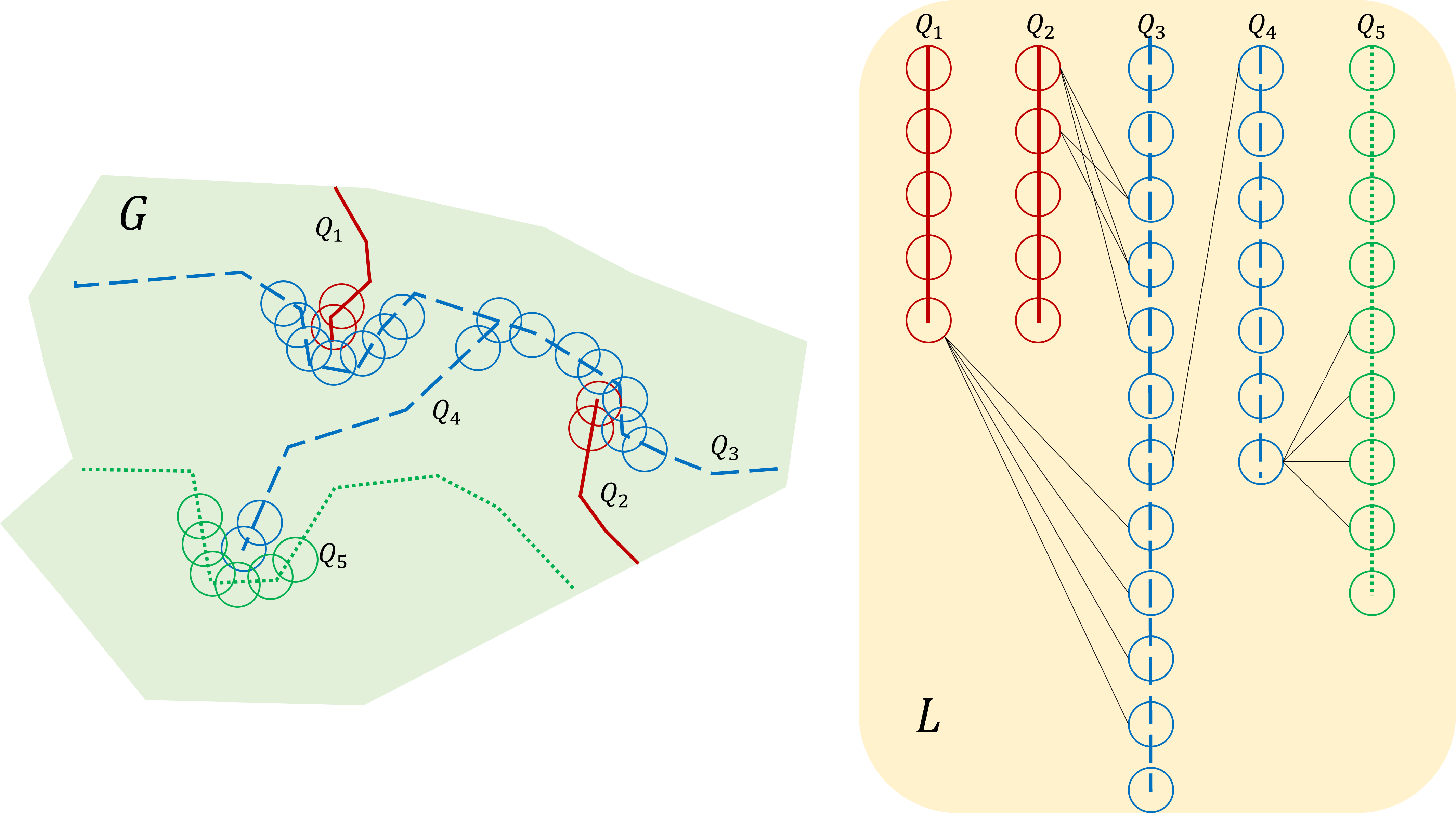
The clusters , that are defined in Definition 10 and in the proof of Lemma 6 (with ), have the property that paths of length at most , that intersect the path separator, are fully contained in one of these clusters, and are well-approximated by a path that goes through the corresponding -landmark. Thus, unifying several clusters and applying Observation 2 on the set of the corresponding landmarks takes care of all the -paths that are contained in these clusters. The remaining challenge is to find a way to divide all the clusters into small sets, such that we will be able to unify the clusters in each set, construct a forest cover to the resulting graph, and then glue forest covers of many different sets together. In terms of the path-clusters graph, this can be formalized using the notion of clustered coloring. This notion has appeared in the literature with several names or formulations, and was mostly studied from a graph-theoretical viewpoint.
Definition 11 ([5]).
Given an undirected graph , a clustered coloring of with colors and block size161616In [5], the block size was called the clustering of the clustered coloring. However, we find the term block size more suitable. E.g., note that when the block size is , a clustered coloring is simply a standard proper coloring of a graph. is a vertex coloring of , in which every monochromatic connected component has at most vertices. More formally, it is a function such that for every color , every connected component in the graph has at most vertices. Here, is the set of vertices colored by , and is the induced graph on .
Next, we argue that for producing tree and forest covers with small stretch and size, one can employ clustered colorings with small parameters for the cluster graphs obtained from path separators on different levels of the recursion.
Lemma 7.
Fix two real parameters , an integer parameter , and a graph on vertices. Suppose that every sub-graph of has a path separator , such that the path-clusters graph of with respect to has a clustered coloring with colors and block size . Then, admits a spanning forest cover , a (not necessarily spanning) tree cover , and an HST cover , all of which of size , such that for every with ,
Proof.
We prove the lemma by induction over (while the other parameters are fixed). For a constant , the claim is trivial. For a general , let be a path separator of , and let be the connected components of , all of which with at most vertices. By the induction hypothesis, every component has a spanning forest cover , a (not necessarily spanning) tree cover , and an HST cover , all with size , such that if , then
By Lemma 2, there is also a forest cover , a (not necessarily spanning) tree cover , and an HST cover171717Lemma 2 only considers forest cover, however, it is immediate to generalize it to hold also for HST covers. For this purpose, under some arbitrary enumeration of the HSTs in the HST covers of each connected component, one can merge the ’th HST of each of them, for every , by simply setting all their roots as children of a new root with label , or . A more explicit construction appears at the end of the proof of Theorem 8. , all with size , such that whenever ,
| (12) |
Next, denote by the path-clusters graph of with respect to . Fix some color . In the graph that is induced by the clusters (vertices of ) colored by , we consider a connected component . Note that the number of clusters in is at most , by the properties of the clustered coloring . Consider the graph that is induced by the union of all clusters in , i.e., . We now apply Lemma 4 on with the demand set (recall that is the center of the cluster ), and obtain a spanning forest cover , a (not necessarily spanning) tree cover , and an HST cover , all with size , as . By Observation 2, for every two vertices in , and any ,
Consider all connected components of . By the definition of the path-clusters graph , clusters do not intersect in if they are not neighbors in . This implies that the sub-graphs of , for every connected component of , are pairwise vertex disjoint, and so are the covers and . By Lemma 2,181818Technically, to apply Lemma 2, we have to consider a sub-graph of , which is the disjoint union of the graphs , without any edges that connect the different graphs . the graph admits a spanning forest cover , a (not necessarily spanning) tree cover , and an HST cover , all with size , such that for every two vertices in the same graph (for a connected component of ), and every ,
| (13) |
We finally can define the desired covers as
The size of each of the covers defined above is bounded by
as desired.
Fix two vertices with . If there is a shortest - path that does not intersect , then we have , and by (12), we get
Otherwise, we fix a shortest (with respect to ) - path , which must intersect . Let be the smallest index such that intersects a path from . Let be a vertex in which and intersect, and let be the -landmark on that is the closest to . In the same way as in the proof of Lemma 6, it is easy to prove that (using Lemma 5). Recall that . This implies that is in the cluster , and in fact, so are all the vertices of , since
We also conclude that the distance between and in the sub-graph induced by is at most
| (14) |
where the step holds since is on the shortest path , which is fully contained in .
Suppose that the cluster is colored by in the clustered coloring , i.e., , and is in a connected component of . Then, in the graph we have
Using this result, applying Inequality (13) with gives
∎
Lemma 7 reduces the problem of finding a forest cover (or a tree cover, or an HST cover) in path-separable graphs to finding a clustered coloring of its corresponding path-clusters graph. In fact, Lemma 6 can be viewed as an application of Lemma 7, where one colors the clusters of each one of the paths alternately by distinct colors, using distinct colors for different paths. This results in a clustered coloring with colors and block size . Then, each demand set consists of only one landmark. Thus, applying Lemma 4 (with ) actually provides a shortest path tree rooted at this landmark (w.l.o.g.). Setting , we obtain Lemma 6.
Next, we show that for -path-separable graphs, there always exists a clustered coloring with colors and block size in . Using Lemma 7, this will lead to a forest cover with larger stretch than in Theorem 9, but with a significantly smaller number of forests.
Lemma 8.
Let be an -vertex -path-separable graph, and let be a path separator such that consists of at most shortest paths in . Fix two parameters and denote . Then, the path-clusters graph of with respect to and has a clustered coloring with colors and block size .
Proof.
Denote by the path-clusters graph of with respect to and . Recall that the vertices of are all the clusters of the form , for some , where is the ’th -landmark (see Lemma 5) on the path from . Denote by the sub-graph of that is induced by such clusters , where is a path from . Note that the ’s are pairwise vertex disjoint (for and paths from and from , respective clusters may intersect in as subsets of , but is a vertex of , and is a vertex of ). We construct a clustered coloring of by focusing on a different each time, and using a distinct palette of colors for each of them. This results in colors overall.
Fix an index . Given a cluster in and an integer , we define the -ball
Note that the graph is unweighted, thus the notation stands for the unweighted distance (i.e., the smallest number of edges on a path) between and in .
Next, we argue that for every cluster and radius , we have the following bound on the size of its ball with radius .
| (15) |
Indeed, given a path in and its -landmarks , suppose that there is an index such that . Let be a path in from to , such that . Note that the radius of each cluster in this path, as a sub-graph of , is at most , and therefore there is a path in from to – the center of – with weight at most . Let be the lowest index such that , and let be the highest index such that . Using the bound we proved for the distances from the landmarks to , we conclude that . See Figure 4 for an illustration. By Lemma 5, the number of landmarks on is at most
Here we used the fact that , and that is a shortest path in , and therefore is the shortest path between . We conclude that there are at most clusters in that are centered in landmarks of , and therefore there are at most clusters in (since there are at most paths in ).

We proceed with a standard ball-carving technique [49, 9, 32]. We iterate over the colors , starting with . Fix an arbitrary cluster and consider the product
For simplicity, we assume here that is an integer number. At least one of the terms in this product must be bounded by the geometric mean, i.e., there is with
Here we used the bound , where . Analyzing the latter function of , one can show that it is decreasing for every , thus its maximum value is obtained when .
We color the clusters in by the color and remove all the clusters of the padded ball from the graph . After the deletion of these clusters, inequality (15) still holds, and we repeat the process with the remaining clusters of (each time coloring clusters by the same color ). When all the clusters of are removed, we move on to the next color and the graph without the clusters that were already colored. This completes the construction of .
To formalize notations, denote by the remaining graph from after removing the ’th ball on the ’th iteration. The arbitrary cluster that is fixed as center is denoted by and the corresponding radius , such that , is denoted by . That is, the clusters of are colored by , and the clusters of the padded ball are removed from to obtain .
If balls were removed in the ’th iteration, then the padded balls cover all of . We bound the number of clusters colored by the color as follows.
That is, each time we color a fraction of at least of the remaining uncolored clusters in . Hence, the number of colors until all clusters of are colored is at most . To color all clusters in , the coloring uses a total of colors.
Finally, notice that each ball that we colored by , for every and , is a connected component in , since neighboring vertices of this ball are immediately removed from (as they are in the padded ball ), and are not colored by . Using Inequality (15), we conclude that these connected components have at most
clusters each, and this is a bound on the block size of the clustered coloring .
∎
In the next lemma we consider tree-like -path-separable graphs, where all the path separators in a single union are rooted at the same vertex. We devise a better clustered coloring of the path-clusters graph for this important case (that includes, e.g., -minor-free graphs).
Lemma 9.
Let be an -vertex tree-like -path-separable graph, and let be a path separator such that consists of at most shortest paths in with a common root . Fix two parameters and denote . Then, the path-clusters graph of with respect to and has a clustered coloring with colors and block size .
Proof.
Similarly to the proof of Lemma 8, given the path-clusters graph of with respect to and , we define a coloring for each sub-graph of , that contains the clusters that are centered on a path from .
Fix an index . For every shortest path in , let be the -landmarks of from Lemma 5. Recall that the sub-graph consists of clusters of the form , for a shortest path in .
We define the color of any cluster in using the distance of , the center of this cluster, to the common root (which is an endpoint of ).
That is, the color that sets to the cluster is the remainder when dividing by . Clearly, the clustered coloring uses at most different colors for , i.e., at most colors for the entire path-clusters graph .
Fix two separator paths in , a landmark on and a landmark on . Suppose that and intersect each other, and let . Recall that have a common endpoint . Then, by the triangle inequality,
Therefore, we have
and thus . Hence, by the definition of , if the two clusters have the same color , i.e., then it must be that . This implies that for any color , and any connected component in , all the clusters in have the same value of .
Fix a color and a connected component of . Given a path in , let be the lowest index such that is in , and let be the highest index such that is in . The argument above shows that , and therefore
where we used the fact that is an endpoint of , and is a shortest path in . By Lemma 5, the number of landmarks in is at most , and therefore the number of the clusters in that are centered on is at most . This shows that the component has at most clusters overall, i.e., the clustered coloring has block size at most .
∎
We now apply the reduction from Lemma 7, to obtain the following corollaries.
Corollary 4.
Let be an -vertex -path-separable graph, let and be real parameters, and let be an integer parameter. Then, admits a spanning forest cover , a (not necessarily spanning) tree cover , and an HST cover , each of them with size , and for every with ,
If is tree-like -path-separable, then the size of these covers is .
The covers from Corollary 4 provide low stretch for pairs of vertices such that , for any given . To obtain low stretch for all pairs of vertices in the graph, we apply them on different scales . As in Section 5.3, if we consider every scale , for , we obtain covers with size (for the tree-like case) and low stretch (, and for a spanning forest cover, not necessarily spanning tree cover and HST cover, respectively). To get rid of the dependence on the aspect ratio , and replace by , we use the same reduction that we used in the proof of Theorem 9, that is presented in Appendix B.
Theorem 10.
Let be an -vertex -path-separable graph, let be a real parameter and let be an integer.
-
1.
has a spanning forest cover with stretch , a (not necessarily spanning) tree cover with stretch , and an HST cover with stretch , all of them with size
If is connected, then by Observation 1, also has a spanning tree cover with the same size and stretch .
-
2.
If is tree-like -path-separable, then the size of all these covers improves to
Note that for not-tree-like -path-separable graphs, one can replace the parameter by , then the size of the covers in Theorem 10 becomes , while the stretch grows by a factor of at most . In particular, the stretch of the spanning forest/tree cover remains .
Recall that -minor-free graphs are (weakly) tree-like -path-separable, for and , where , and that graphs with bounded genus are strongly tree-like -path-separable (see Items (2) and (3) in Theorem 3). Thus, the following corollary is derived by Theorem 10.
Corollary 5.
Let be an -vertex graph, and let be an integer.
-
1.
If is -minor-free, then it has a spanning forest cover with stretch , and a (not necessarily spanning) tree cover and an HST cover , both with stretch . Each of the covers and has size
If is connected, then by Observation 1, also has a spanning tree cover with the same size and stretch .
-
2.
If has bounded genus , then it has a spanning forest cover with stretch , and a (not necessarily spanning) tree cover and an HST cover , both with stretch . Each of the covers and has size
If is connected, then by Observation 1, also has a spanning tree cover with the same size and stretch . The result applies for both orientable and non-orientable genus.
6 Path-Reporting Spanners and Emulators
In this section, we show how tree covers give rise to path-reporting spanners and emulators. Spanners and emulators are well-studied objects (see Definition 2 for a formal definition). In this section we provide results for the stronger notions of path-reporting spanners/emulators (see Definition 3).
For the special case where the given graph is a tree, we next prove a useful fact, that admits a path-reporting spanner with optimal stretch, query time and size (, and , respectively). For this purpose, we use the following result by Harel and Tarjan [41].
Theorem 11 ([41]).
For every rooted tree on vertices there is an oracle with size , that given two vertices in , returns their lowest common ancestor (LCA) in within time.
Lemma 10.
Let be an undirected weighted tree with vertices. There is a path-reporting -spanner with constant query time and size .
Proof.
First, note that the set of underlying edges (in which all the output paths of must be contained) must be exactly , the edges of . The size of this set is .
Next, we construct the oracle . For an arbitrary chosen root , the oracle stores, for every , the distance and the parent of in (i.e., the next vertex on the unique path from to the root ). In addition, stores the LCA oracle from Theorem 11, for the rooted tree . Since the size of is , the total size of is also .
Given a query , the oracle invokes the LCA oracle to find the LCA of in . Then, the distance is computed within time by
If a - path is also required, the oracle uses the pointers , starting from , until it gets to . The concatenation of these two paths is the unique path in between . The time for this computation is proportional to the number of edges in the output path.
∎
Applying Lemma 10 on every tree of a given tree cover produces a path-reporting emulator (if the tree cover is non-spanning) or a path-reporting spanner (if the tree cover is spanning). The following lemma provides a formal argument.
Lemma 11.
Let be an undirected weighted graph, let be a set of vertex pairs, and let be a -pairwise tree cover for with stretch , (maximum) overlap and average overlap . Then, the graph has a -pairwise path-reporting -emulator with query time and size . Moreover, if is a spanning tree cover, then is a -pairwise path-reporting spanner with the same properties.
Proof.
Given the tree cover , for every , construct the path-reporting -spanner from Lemma 10 (here, is simply , the edges of the tree ). We define an oracle to contain all the oracles for . In addition, for every , the oracle contains a list of pointers to all trees such that .
Given a query , the oracle iterates over all trees that appear both in and in . For every such tree , using the oracle , the oracle computes the distance estimate , within time . This way, the tree with minimal value of is found. As is a -pairwise tree cover with stretch , this value is always at least , and if , it is at most . Lastly, the oracle returns either the distance estimate , within time , or a path in with weight , within time . Note that the total query time of is if an output path is not required, or if an output path is required.
By Lemma 10, the size of each oracle is . Hence, the size of is
by the definition of the average overlap (see Definition 8).
Note that all of the output paths of are contained in the union . Thus, we define the set of underlying edges to be this union. The size of is
We conclude that is a path-reporting -emulator with query time and size . If is a spanning tree cover, then by definition, it means that for all . Thus, , i.e., is a path-reporting spanner.
∎
Lemma 11 provides a unified framework of converting tree covers into path-reporting emulators and spanners. In fact, one can verify that the well known results by [59] and [52] can be achieved using this framework (however, with an improved query time that relies on their specific constructions).
We proceed by applying Lemma 11 on our new tree covers in this paper. By applying Lemma 11 on Corollary 1, we obtain the following theorem.
Theorem 12.
Let be an undirected weighted graph on vertices. Given an integer parameter , there exists a path-reporting spanner with stretch , query time and size .
Remark 1.
Theorem 13.
Let be an -vertex undirected weighted -vertex-separable graph, for some non-decreasing function . Let be an integer parameter, and denote . Then, has a path-reporting emulator with stretch , and a path-reporting spanner with stretch , both with query time and size .
The following corollaries are obtained by setting , for some , and setting , for some function of . They are analogous to Corollaries 2 and 3.
Corollary 6.
Let be an -vertex -vertex-separable graph, for , for some , and let be an integer. Then, has a path-reporting emulator with stretch , and a path-reporting spanner with stretch , both with query time and size .
Corollary 7.
Let be an -vertex graph with treewidth , and let be an integer. Then, admits a path-reporting emulator with stretch , and a path-reporting spanner with stretch , both with query time and size .
These results for path-reporting emulators improve upon previous bounds on the size-stretch tradeoff [59, 52, 31, 17] when , for a sufficiently small constant . For path-reporting spanners, our results improve upon existing state-of-the-art bounds for this tradeoff [31, 17, 59, 19] for . Note, however, that our query time is inferior to that of [59, 52, 31, 17, 19].
Applying Lemma 11 on Theorem 9 for -path-separable graphs provides a path-reporting spanner with stretch , and query time and size overhead (i.e., size divided by ) . Next, we use a more subtle construction that employs the fact that the tree cover from Theorem 9 consists of a different tree cover for each scale. To determine which scales should be used, we employ the tree cover of Gupta et al. [38]. This eliminates one of the factors from the query time of the resulting path-reporting spanner.
Theorem 14.
Let be an -vertex -path-separable graph, let be an integer parameter and let be a real parameter. Then, admits a path-reporting spanner with stretch , query time , and size .
Proof.
For simplicity, we show a path-reporting spanner with size , instead of . To obtain the latter, we apply our new aspect ratio reduction (see Appendix B.1). Here, as well as in Appendix B.1, we assume that , as otherwise we multiply the weight of each edge by . Then, the aspect ratio is simply the diameter . We also assume that the graph is connected, as otherwise we construct a path-reporting spanner for every connected component, and their union is the desired path-reporting spanner for .
In this proof we use the following result of [38], for tree covers of path-separable graphs.
Theorem 15 ([38]).
Every -vertex -path-separable graph admits a (spanning) tree cover with stretch and size .
Applying Lemma 11 on this tree cover by [38] (with ), we obtain a path-reporting -spanner with query time and size .
For every , let be the forest cover from Lemma 6, for . By Observation 1, for every there is also a tree cover for with the same properties. That is, the size of is , and for every such that , there is a tree with . This implies that is a -pairwise tree cover with stretch , for the set of vertex pairs . Indeed, for every pair we have , thus there is a tree with
We apply Lemma 11 on , and obtain a -pairwise path-reporting -spanner for with query time and size . In our new path-reporting spanner , we define , and we store all the oracles in .
Given a query , the oracle first applies on , to get an estimate , within time . Equivalently, we have . Then, the oracle finds all the indices such that the interval intersects the interval . We claim that there are at most three such values . Indeed, if and are both in , for some , then
i.e., . Hence, there is an index such that , or equivalently, . Thus, one of the oracles outputs a distance estimate for with stretch at most . The oracle applies these oracles on and finds the index such that outputs the minimal distance estimate for . If a path is also required, applies on to obtain such an approximate path. In both cases, has stretch at most .
Note that the query time of equals the query time of plus the query times of and . As these are all , the query time of is as well.
Lastly, observe that the output paths of are all in , and that the size of and of are both at most the total size of the oracles , which is .
∎
Consider Theorem 10, in which we presented tree covers for -path-separable graphs with stretch and sublinear size in . Applying Lemma 11 on this theorem provides the following result.
Theorem 16.
Let be an -vertex -path-separable graph, let be an integer parameter and let be a real parameter. Then, admits a path-reporting spanner (respectively, emulator) with stretch (resp., ), query time (resp., ), and size (resp., ). If is also tree-like -path-separable, then improves to and improves to .
A similar proof as the proof of Theorem 14 improves the query time of these path-reporting spanners and emulators to . For tree-like separators, the bound improves to . To find the right scale, we use the distance oracle that is implied by Theorem 16, with . The proof of the following result is in Appendix B.2
Theorem 17.
Let be an -vertex -path-separable graph, let be an integer parameter and let be a real parameter. Then, admits a path-reporting spanner (respectively, emulator) with stretch (resp., ), query time (resp., ), and size (resp., ). Here, if is also tree-like -path-separable, and otherwise .
Recall that -minor-free graphs are (weakly) tree-like -path-separable, for and , where , and that graphs with bounded genus are strongly tree-like -path-separable (see Items (2) and (3) in Theorem 3). Thus, the following corollaries are derived by Theorems 14 and 17.
Corollary 8.
Let be a -minor-free -vertex graph and let be an integer parameter. Recall that .
-
1.
has a path-reporting spanner with stretch , query time and size .
-
2.
has a path-reporting spanner with stretch , and a path-reporting emulator with stretch , both with query time and size .
Corollary 9.
Let be an -vertex graph with bounded genus , let be an integer parameter and let be a real parameter.
-
1.
has a path-reporting -spanner with query time and size .
-
2.
has a path-reporting spanner with stretch , query time , and size .
-
3.
has a path-reporting emulator with stretch , query time
, and size .
6.1 Path-Reporting Spanners with Improved Stretch
Consider our new path-reporting spanners for general graphs (Theorem 12), vertex-separable graphs (Theorem 13) and path-separable graphs (Theorems 14 and 17). In almost all these results, the stretch depends, albeit very mildly, on the parameters of the separators. Namely, the stretch is generally , where is the size of the recursive separators, the number of separator paths, or, in general graphs, simply . An exception is the path-reporting spanner with stretch for -path-separable graphs (see Theorem 14); however, the dependency on in the size and query time is linear (i.e., it is ).
In this section, we apply techniques from [31] on our new path-reporting emulators, to convert them into path-reporting -spanners, while only losing small factors in the size. Specifically, we use the following theorem from [31].
Theorem 18 ([31], Theorem 3 and Remark 1).
Given an undirected weighted graph , an integer , a positive parameter , and a set of pairs , there exists a path-reporting -pairwise -spanner with query time and size
where .
In addition, there exists a path-reporting -pairwise -spanner with query time and size
In the next lemma, we apply the pairwise path-reporting spanners from Theorem 18 on a path-reporting emulator, to obtain a path-reporting spanner (for all queries ).
Lemma 12.
Let be an undirected weighted -vertex graph, and suppose that admits a path-reporting emulator with stretch , query time and size , for some integer parameters . Suppose also that . Then, for every , the graph admits a path-reporting spanner with stretch , query time and size
where and .
In addition, admits a path-reporting spanner with stretch , query time and size
Proof.
Given the path-reporting emulator , we construct a path-reporting spanner as follows. Consider the set as a set of pairs (formally, we insert the pairs to , for every ). Let be the resulting path-reporting -pairwise -spanner (resp., -spanner) from Theorem 18. We define an oracle , that receives a query , and applies the oracle to obtain an estimate . If a - path is also required, the oracle obtains a - path in (again by applying ), the applies the oracle on every edges of , and finally concatenates the resulting paths in into a single - path in .
It is immediate to verify that the query time of the resulting path-reporting spanner is . To analyze the stretch of , let be any query, and suppose that a - path is required (otherwise, the stretch is at most , as in the path-reporting emulator ). Then, the - path obtained by has weight . Replacing every edge of by a path in of stretch or results in a - path in with stretch or , respectively.
In the former case, where has stretch , it has size , where . We choose (for the given parameters ), and obtain a path-reporting spanner with size
Here we used the assumptions that and .
In the latter case, where has stretch , it has size . We again choose , and a constant , and obtain a path-reporting spanner with size
∎
Lemma 12, when applied to our path-reporting emulators from Theorems 13 and 17, provides the following results for path-reporting spanners.
Theorem 19.
Let be an undirected weighted -vertex graph, let be any integer parameter and let be any real parameter. In what follows, we denote , for any parameter .
-
1.
Suppose that is -vertex-separable, for some non-decreasing function , and denote . Then, admits a path-reporting spanner with stretch (resp., ), query time and size (resp., ), where .
In particular, if , for a constant , then , and if the graph has treewidth , then .
-
2.
Suppose that is -path-separable. Then, admits a path-reporting spanner with stretch , query time and size , where . Here, if is also tree-like -path-separable, and otherwise.
-
3.
Suppose that is -path-separable. Then, admits a path-reporting spanner with stretch , query time and size ), where . Here, if is also tree-like -path-separable, and otherwise.
Recall that -minor-free graphs are (weakly) tree-like -path-separable, for and , where , and that graphs with bounded genus are strongly tree-like -path-separable (see Items (2) and (3) in Theorem 3). Thus, the following corollary is derived by Theorem 19.
Corollary 10.
Let be an undirected weighted -vertex graph, let be any integer parameter and let be any real parameter. In what follows, we denote , for any parameter .
-
1.
Suppose that is -minor-free. Then, admits a path-reporting spanner with stretch , query time and size , where .
-
2.
Suppose that has bounded genus . Then, admits a path-reporting spanner with stretch , query time and size , where .
-
3.
Suppose that has bounded genus . Then, admits a path-reporting spanner with stretch , query time and size ), where .
6.2 Distance Oracles with Improved Stretch
Recall that Theorem 13 provides a path-reporting emulator with stretch , query time and size , for any -vertex graph that is -vertex-separable, and any integer parameter . Here, we provide an improved stretch of . We note, however, that the structure that achieves this bound is not a path-reporting emulator, but only a distance oracle. That is, given a query , this structure outputs only an estimate that satisfies , but not a path with weight in a fixed small-size emulator of (see Definition 4). The proof of the following theorem is in Appendix C.
Theorem 20.
Let be an -vertex undirected weighted -vertex-separable graph, for a non-decreasing function . Let be an integer, and denote . Then, has a distance oracle with stretch at most , size , and query time .
References
- [1] (2020) Ramsey spanning trees and their applications. ACM Transactions on Algorithms (TALG) 16 (2), pp. 1–21. Cited by: Appendix A, Appendix A, §1.1, §1.1, §1.4, §1.4, §4, §5.1, §5.2, §5.2, Remark 1, Theorem 4.
- [2] (2006) Routing in networks with low doubling dimension. In 26th IEEE International Conference on Distributed Computing Systems (ICDCS’06), pp. 75–75. Cited by: §1.1.
- [3] (2006) Object location using path separators. In Proceedings of the Twenty-Fifth Annual ACM Symposium on Principles of Distributed Computing, PODC 2006, Denver, CO, USA, July 23-26, 2006, E. Ruppert and D. Malkhi (Eds.), pp. 188–197. External Links: Link, Document Cited by: Appendix A, §1.1, §1.2, §1.3, §1.4, Table 2, item 2, Definition 7, footnote 12, footnote 6.
- [4] (1996) Linear algorithms for partitioning embedded graphs of bounded genus. SIAM Journal on Discrete Mathematics 9 (1), pp. 129–150. Cited by: §1.2, item 3.
- [5] (2003) Partitioning into graphs with only small components. Journal of Combinatorial Theory, Series B 87 (2), pp. 231–243. External Links: ISSN 0095-8956, Document, Link Cited by: §1.4, Definition 11, footnote 16.
- [6] (1995) Euclidean spanners: short, thin, and lanky. In Proceedings of the Twenty-Seventh Annual ACM Symposium on Theory of Computing, 29 May-1 June 1995, Las Vegas, Nevada, USA, F. T. Leighton and A. Borodin (Eds.), pp. 489–498. External Links: Link, Document Cited by: §1.5.
- [7] (1992) Routing with polynomial communication-space tradeoff. SIAM J. Discrete Mathematics 5, pp. 151–162. Cited by: §3.
- [8] (1996) Probabilistic approximation of metric spaces and its algorithmic applications. In Proceedings of the 37th IEEE Symp. on Foundations of Computer Science, pp. 184– 193. Cited by: footnote 11.
- [9] (1996) Probabilistic approximation of metric spaces and its algorithmic applications. In Proceedings of 37th Conference on Foundations of Computer Science, Vol. , pp. 184–193. External Links: Document Cited by: §5.4.
- [10] (2022) Covering metric spaces by few trees. J. Comput. Syst. Sci. 130, pp. 26–42. External Links: Link, Document Cited by: Appendix A, Appendix A, §1.1, §1.1, §1.1, §1.1, §1.2, §1.2, §1.4, §1.5, Table 1, Table 1, Table 2, Table 2, Table 2, §5.3.
- [11] (2003) On metric Ramsey-type phenomena. In Proceedings of the 35th Annual ACM Symposium on Theory of Computing, June 9-11, 2003, San Diego, CA, USA, L. L. Larmore and M. X. Goemans (Eds.), pp. 463–472. External Links: Link, Document Cited by: Appendix A, §1.1, §1.1, §2.1, footnote 10, footnote 11.
- [12] (1995) Approximating treewidth, pathwidth, frontsize, and shortest elimination tree. Journal of Algorithms 18 (2), pp. 238–255. Cited by: §2.3.
- [13] (2016) On hierarchical routing in doubling metrics. ACM Trans. Algorithms 12 (4), pp. 55:1–55:22. External Links: Link, Document Cited by: §1.1, §1.5.
- [14] (2023) Covering planar metrics (and beyond): o(1) trees suffice. In 2023 IEEE 64th Annual Symposium on Foundations of Computer Science (FOCS), pp. 2231–2261. Cited by: §1.1, §1.1, §1.1, §1.2, Table 1.
- [15] (2024) Shortcut partitions in minor-free graphs: steiner point removal, distance oracles, tree covers, and more. In Proceedings of the 2024 Annual ACM-SIAM Symposium on Discrete Algorithms (SODA), pp. 5300–5331. Cited by: §1.1, §1.1, §1.1, §1.2, Table 1, Table 2.
- [16] (2025) Light tree covers, routing, and path-reporting oracles via spanning tree covers in doubling graphs. In Proceedings of the 57th Annual ACM Symposium on Theory of Computing, STOC 2025, Prague, Czechia, June 23-27, 2025, M. Koucký and N. Bansal (Eds.), pp. 2257–2268. External Links: Link, Document Cited by: §1.1, §1.1, §1.5.
- [17] (2024) Path-reporting distance oracles with logarithmic stretch and linear size. In 51st International Colloquium on Automata, Languages, and Programming (ICALP 2024), Cited by: §1.3, §6, Remark 1.
- [18] (2013) Compact routing schemes with improved stretch. In ACM Symposium on Principles of Distributed Computing, PODC ’13, Montreal, QC, Canada, July 22-24, 2013, P. Fatourou and G. Taubenfeld (Eds.), pp. 33–41. External Links: Link, Document Cited by: §D.2.
- [19] (2015) Approximate distance oracles with improved bounds. In Proceedings of the Forty-Seventh Annual ACM on Symposium on Theory of Computing, STOC 2015, Portland, OR, USA, June 14-17, 2015, R. A. Servedio and R. Rubinfeld (Eds.), pp. 1–10. External Links: Link, Document Cited by: §6.
- [20] (2025) Lower bounds on tree covers. arXiv preprint arXiv:2508.10376. Cited by: §1.1, §1.5.
- [21] (1998) Fast algorithms for constructing t-spanners and paths with stretch t. SIAM J. Comput. 28 (1), pp. 210–236. External Links: Link, Document Cited by: §1.4.
- [22] (2000) Polylog-time and near-linear work approximation scheme for undirected shortest paths. J. ACM 47 (1), pp. 132–166. External Links: Link, Document Cited by: §1.4.
- [23] (2010) Path separability of graphs. In International Workshop on Frontiers in Algorithmics, pp. 262–273. Cited by: §1.1.
- [24] (1985) A separator theorem for graphs of fixed genus. Serdica 11 (4), pp. 319–329. Cited by: §1.2.
- [25] (1988) Linear algorithms for graph separation problems. In Scandinavian Workshop on Algorithm Theory, pp. 216–222. Cited by: §1.2.
- [26] (2005) On monochromatic component size for improper colourings. Discrete Applied Mathematics 148 (1), pp. 89–105. External Links: ISSN 0166-218X, Document, Link Cited by: §1.4.
- [27] (2021) Ultra-sparse near-additive emulators. In Proceedings of the 2021 ACM Symposium on Principles of Distributed Computing, PODC’21, New York, NY, USA, pp. 235–246. External Links: ISBN 9781450385480, Link, Document Cited by: §1.4.
- [28] (2016) Space-efficient path-reporting approximate distance oracles. Theor. Comput. Sci. 651, pp. 1–10. External Links: Link, Document Cited by: §1.3.
- [29] (2019) Linear-size hopsets with small hopbound, and constant-hopbound hopsets in RNC. In The 31st ACM on Symposium on Parallelism in Algorithms and Architectures, SPAA 2019, Phoenix, AZ, USA, June 22-24, 2019., pp. 333–341. External Links: Link, Document Cited by: §1.4.
- [30] (2016) A linear-size logarithmic stretch path-reporting distance oracle for general graphs. ACM Trans. Algorithms 12 (4), pp. 50:1–50:31. External Links: Link, Document Cited by: §1.3.
- [31] (2023) Path-reporting distance oracles with logarithmic stretch and size o (n log log n). In 2023 IEEE 64th Annual Symposium on Foundations of Computer Science (FOCS), pp. 2278–2311. Cited by: §1.3, §1.3, §2.1, §2.2, §6.1, §6, Lemma 1, Remark 1, Theorem 18.
- [32] (2003) A tight bound on approximating arbitrary metrics by tree metrics. In Proceedings of the thirty-fifth annual ACM symposium on Theory of computing, pp. 448–455. Cited by: §5.4.
- [33] (2025) On sparse covers of minor free graphs, low dimensional metric embeddings, and other applications. In 41st International Symposium on Computational Geometry (SoCG 2025), pp. 49–1. Cited by: Table 3, Table 3, Table 3.
- [34] (2004) Distance labeling in graphs. Journal of algorithms 53 (1), pp. 85–112. Cited by: §D.1.
- [35] (1984) A separator theorem for graphs of bounded genus. Journal of Algorithms 5 (3), pp. 391–407. Cited by: §1.2.
- [36] (2025) Polynomial bounds for the graph minor structure theorem. arXiv preprint arXiv:2504.02532. Cited by: §1.1, Table 2, item 2.
- [37] (2006) Oblivious network design. In Proceedings of the seventeenth annual ACM-SIAM symposium on Discrete algorithm, pp. 970–979. Cited by: §1.1.
- [38] (2004) Traveling with a pez dispenser (or, routing issues in MPLS). SIAM J. Comput. 34 (2), pp. 453–474. External Links: Link, Document Cited by: §B.1, §1.1, §1.1, §1.1, §1.2, §1.2, §1.3, §1.4, §1.4, Table 1, Table 2, Table 2, Table 3, Table 3, Table 3, §5.3, §6, §6, §6, Theorem 15.
- [39] (2003) Tree based mpls routing. In Proceedings of the fifteenth annual ACM symposium on Parallel algorithms and architectures, pp. 193–199. Cited by: §1.1.
- [40] (2001) Steiner points in tree metrics don’t (really) help. In Proceedings of the Twelfth Annual Symposium on Discrete Algorithms, January 7-9, 2001, Washington, DC, USA, S. R. Kosaraju (Ed.), pp. 220–227. External Links: Link Cited by: Appendix A, §2.1.
- [41] (1984) Fast algorithms for finding nearest common ancestors. SIAM Journal on Computing 13 (2), pp. 338–355. External Links: Document, Link, https://doi.org/10.1137/0213024 Cited by: §6, Theorem 11.
- [42] (2022) Can’t see the forest for the trees: navigating metric spaces by bounded hop-diameter spanners. In Proceedings of the 2022 ACM Symposium on Principles of Distributed Computing, pp. 151–162. Cited by: §3.
- [43] (2011) Linear-space approximate distance oracles for planar, bounded-genus and minor-free graphs. In Automata, Languages and Programming: 38th International Colloquium, ICALP 2011, Zurich, Switzerland, July 4-8, 2011, Proceedings, Part I 38, pp. 135–146. Cited by: §1.3, footnote 6.
- [44] (2020) Quickly excluding a non-planar graph. arXiv preprint arXiv:2010.12397. Cited by: §1.1.
- [45] (1997) A randomized parallel algorithm for single-source shortest paths. J. Algorithms 25 (2), pp. 205–220. External Links: Link, Document Cited by: §1.4.
- [46] (2002) Preprocessing an undirected planar network to enable fast approximate distance queries. In Proceedings of the thirteenth annual ACM-SIAM Symposium on Discrete Algorithms, pp. 820–827. Cited by: §1.2, §1.3, §1.4, §1.4, §5.3.
- [47] (1997) Storage management for evolving databases. In Proceedings 38th Annual Symposium on Foundations of Computer Science, Vol. , pp. 353–362. External Links: Document Cited by: §1.4.
- [48] (2001) On approximating planar metrics by tree metrics. Information Processing Letters 80 (4), pp. 213–219. Cited by: §2.1.
- [49] (1993) Decomposing graphs into regions of small diameter. Combinatorica 13, pp. 441–454. Cited by: §5.4.
- [50] (1979) A separator theorem for planar graphs. SIAM Journal on Applied Mathematics 36 (2), pp. 177–189. Cited by: item 1.
- [51] (1996) On the distortion required for embedding finite metric spaces into normed spaces. Israel Journal of Mathematics 93 (1), pp. 333–344. Cited by: §D.1.
- [52] (2007) Ramsey partitions and proximity data structures. Journal of the European Mathematical Society 9 (2), pp. 253–275. Cited by: Appendix A, §1.1, §1.1, §1.4, §1.4, §4, §6, §6, Theorem 6, footnote 15, footnote 4.
- [53] (2012) Scale-oblivious metric fragmentation and the nonlinear Dvoretzky theorem. Israel Journal of Mathematics 192, pp. 489–504. Cited by: Appendix A, Appendix A, §1.1, §4, Theorem 5, footnote 4.
- [54] (2024) Path-Reporting Distance Oracles with Linear Size. In 19th Scandinavian Symposium and Workshops on Algorithm Theory (SWAT 2024), H. L. Bodlaender (Ed.), Leibniz International Proceedings in Informatics (LIPIcs), Vol. 294, Dagstuhl, Germany, pp. 36:1–36:16. Note: Keywords: Graph Algorithms, Shortest Paths, Distance Oracles External Links: ISBN 978-3-95977-318-8, ISSN 1868-8969, Link, Document Cited by: §1.3.
- [55] (2000) Informative labeling schemes for graphs. In Mathematical Foundations of Computer Science 2000, 25th International Symposium, MFCS 2000, Bratislava, Slovakia, August 28 - September 1, 2000, Proceedings, M. Nielsen and B. Rovan (Eds.), Lecture Notes in Computer Science, Vol. 1893, pp. 579–588. External Links: Link, Document Cited by: §D.1, Theorem 21.
- [56] (2000) Proximity-preserving labeling schemes. Journal of Graph Theory 33 (3), pp. 167–176. Cited by: §D.1, Theorem 21.
- [57] (1986) Graph minors. v. excluding a planar graph. Journal of Combinatorial Theory, Series B 41 (1), pp. 92–114. Cited by: item 2.
- [58] (2003) Graph minors. xvi. excluding a non-planar graph. Journal of Combinatorial Theory, Series B 89 (1), pp. 43–76. Cited by: §1.1, item 2.
- [59] (2001) Approximate distance oracles. In Proc. of the 33rd ACM Symp. on Theory of Computing, pp. 183–192. Cited by: §D.1, §1.3, §3, §6, §6.
- [60] (2001) Compact routing schemes. In Proceedings of the Thirteenth Annual ACM Symposium on Parallel Algorithms and Architectures, SPAA ’01, New York, NY, USA, pp. 1–10. External Links: ISBN 1-58113-409-6, Link, Document Cited by: §D.2, §3, Theorem 23.
- [61] (2004) Compact oracles for reachability and approximate distances in planar digraphs. Journal of the ACM (JACM) 51 (6), pp. 993–1024. Cited by: §1.2, §1.3, §1.4, §1.4, §1.4, §1.4, §1.4, Table 3, Table 3, item 1, §5.3, footnote 7.
- [62] (2012) Defective and clustered graph colouring. The Electronic Journal of Combinatorics, pp. DS23–Apr. Cited by: §1.4.
- [63] (2013) Approximate distance oracles with improved query time. In Proceedings of the Twenty-Fourth Annual ACM-SIAM Symposium on Discrete Algorithms, SODA 2013, New Orleans, Louisiana, USA, January 6-8, 2013, S. Khanna (Ed.), pp. 539–549. External Links: Link, Document Cited by: §1.3.
Appendix A Comparison with Constructions for General Graphs
It is instructive to compare our HST covers for -vertex-separable graphs (or graphs with treewidth ) with the HST covers of [52, 53]. For a parameter , our HST cover has stretch and size . The HST cover of [53] for general graphs has the same stretch and size . Hence, for any constant , our HST cover has smaller size as long as , i.e., our result provides a graceful generalization of the result of [53], parametrized by . This is also the case for our non-spanning and spanning tree covers for this graph family. Their stretch is and , respectively, with the same constants hidden by the -notation as in the respective state-of-the-art non-spanning and spanning tree covers for general graphs. Note that the tree covers of [52, 53, 1] are Ramsey ones (for general graphs), while our tree covers are not. Recall that a lower bound of [10, 11] rules out existence of Ramsey tree covers with stretch and size already for series-parallel graphs (that have treewidth ).
For strongly -path-separable graphs, our HST cover has stretch and size . For constant , this bound improves the bound for general graphs for , and this is also the case when comparing our non-spanning and spanning tree covers with the state-of-the-art bounds of [53, 40] and [1], respectively.
For weakly -path-separable graphs, our bounds leave larger room for improvement. Specifically, the size of our tree covers grows linearly with , while ideally it should be proportional to . Note, however, that the prime example of weakly -path-separable graph is the class of -minor-free graphs. The separator theorem of [3] provides these graphs with a weakly tree-like -path separator with (in particular, for ) and (the total number of paths in their separator is also at most ). Observe that for this graph class, is much smaller than , , and thus our bound of on the size of our tree cover is much smaller (for and ) than the previously known bound of on the size of the stretch- non-spanning tree covers for these graphs [10].
Appendix B Aspect Ratio Reduction
Recall that the spanning forest covers from Lemma 6 and the covers from Corollary 4 provide low stretch only for pairs of vertices with , for a given scale . In each of these results, constructing a cover for each relevant scale of the form , and unifying these covers, provides a cover with low stretch for all pairs , at the cost of multiplying the size by . For weighted graphs, the aspect ratio may be very large, thus the resulting size may be large as well.
In this appendix, we merge the covers for different scales in a more subtle way. See the discussion at the end of Section 1.4 for some intuition. As a result, their size is only multiplied by a factor of , rather than . This improves the naive construction whenever . We start with (spanning and non-spanning) forest covers.
Lemma 13.
Let be an -vertex undirected weighted graph, and let and be real parameters. Suppose that, for every , every minor of admits a forest cover with size at most , such that for every with there is a forest with . Then, admits a forest cover with size at most and stretch . Moreover, if for every minor and the forest cover is spanning, then is a spanning forest cover for .
Proof.
We assume that , as otherwise we multiply the weight of each edge by . Then, the aspect ratio is simply the diameter .
Fix some , and consider the sequence
In the proof, we will show the existence of a -pairwise forest cover for (see Definition 8), with size at most and stretch , for the set of pairs
As we will prove below, unifying these pairwise forest covers, for different values of , produces the desired forest cover for . To construct the pairwise forest cover , we prove the following claim by induction over .
Claim 1.
Given a graph and a positive parameter , for every integer there is a -pairwise forest cover for , with size and stretch , where
Moreover, if for every minor and the forest cover is spanning, then is a spanning forest cover too.
Proof.
For , consider the sub-graph , that is obtained from by removing all edges of weight greater than . This sub-graph (which is also a minor of ) has a forest cover of size at most , such that whenever , there is a forest with . For we have . In particular, the edges of any shortest - path in are of weight at most , and therefore they exist in the sub-graph , and . Hence, there is a forest with
This shows that is a -pairwise forest cover with size at most and stretch , thus proving the induction basis.
Next, fix some . Consider the minor that is obtained from by removing edges with a weight greater than , and contracting the edges with weight at most . For every vertex in , let be a sub-graph of , where is the set of vertices in that are contracted into in , and are the edges of with weight at most between vertices of . Note that is a connected graph, since its vertices and edges were all contracted to the same vertex .
Let be a forest cover for , with size at most , such that if satisfy , then there is a forest with .
For every vertex , we apply the induction hypothesis on the graph , and obtain a -pairwise forest cover with size at most and stretch at most . By Observation 1, there is also a -pairwise tree cover for , with the same size and stretch, which is spanning if is spanning. The latter happens, in particular, if for every minor and the forest cover is spanning, as implied by the induction hypothesis.
We now merge the forest cover (for the graph ) with the pairwise tree covers (for the graphs ), for every . Under some arbitrary enumeration of the forests in these covers, let be the ’th forest of , and let be the ’th tree of , for every vertex in . Here, since the sizes of and are at most , the index is at most . If there are less than forests in , we arbitrarily assign . Similarly, if for some the size of is less than , we define .
Fix some index and consider the forest . Recall that is not necessarily a spanning forest of the minor . That is, every edge of may exist in or not. In the former case, this edge originates at some edge of , with the same weight , such that and were contracted to and , respectively (i.e., and ). In the latter case, fix two arbitrary vertices and and define a new edge with weight . In both cases, we say that the edge corresponds to the edge , and vice versa.
We are now ready to define the merged forest . This forest consists of all the corresponding edges to the edges of , and of the edges of the trees , for every . Note that is a forest with vertices in , i.e., a (not necessarily spanning) forest of . Moreover, if and are spanning, then is a spanning forest of . To observe that is indeed a forest, note that it cannot contain a cycle in any of the trees , so if there is a cycle in , a subset of its edges corresponds to a cycle in , in contradiction to being a forest. The desired forest cover is now defined as
Fix some . To analyze the stretch of for the pair , we consider two cases. First, if , then it means, in particular, that , and therefore there is a shortest - path in that consists only of edges with weight at most . In the graph , this entire path is contracted to the same vertex . Thus, it is fully contained in the graph , and we have
for some . Since is a -pairwise tree cover with stretch , where is defined over the graph , we conclude that there is a tree (where is the ’th tree of ) with
The forest contains , and thus as well.
The second case is that , i.e., . Suppose that and were contracted to vertices and , respectively, in the minor . Since , every edge on the shortest - path in is either contracted or present in , and therefore . Thus, by our assumption on the forest cover , there is a forest (which is the ’th forest in ) such that
| (16) |
Consider the unique - path in , which has weight . For every , the edge corresponds to some edge , where and . Denoting and , we can say that for every . For every , recall that is a tree in the tree cover . Thus, it contains a path between and , such that every edge on is an edge of , or has weight . In both cases, the weight of the edge is the weight of some simple path in , and thus bounded by (since, by definition, all edges in have weight at most ). This proves that the weight of the path is at most .
Concatenating the paths , for every , with the edges , for every , we obtain a - path in . To bound its weight, we analyze the weight of an edge , for some . Recall that this edge corresponds to the edge of . If the forest is spanning, then is an edge of , and we have . Otherwise, this weight was defined as . Consider an - simple path in that follows the edges that correspond to the edges in the shortest - path in , and connects any two of them with an arbitrary simple path in an appropriate graph . These simple paths have a total of at most edges (of ), each of weight at most , by the definition of the graphs . Thus, , and therefore the weight of is . Since in non-spanning forest covers, the weight of each edge is at least the distance between its endpoints, we conclude that .
In both cases above, of being spanning or non-spanning, we obtained the bound on the weight of every edge of the form , , that participates in the path in the forest . Using this bound, we get
In conclusion, we saw that whenever , the forest cover , that has size at most , has a forest with . We conclude that is a -pairwise forest cover with stretch and size at most .
∎
Next, we note that for , every have , and therefore . By Claim 1, there is a -pairwise forest cover with size at most and stretch . Moreover, by Claim 1, this forest cover is spanning if is spanning.
We define
where is the pairwise forest cover with . Since the size of each is at most , the size of the forest cover is .
To analyze the stretch of , fix some . There is a unique index such that . Then, there is a unique index such that . Denoting , we have
Thus, , and there is a forest with .
We conclude that has stretch at most and size at most , and that it is a spanning forest cover if is a spanning forest cover for every minor and every . Replacing by , we obtain the desired result.
∎
Next, we prove an analogous lemma to Lemma 13 for HST covers.
Lemma 14.
Let be an -vertex undirected weighted graph, and let and be real parameters. Suppose that, for every , every minor of admits an HST cover with size at most , such that for every with there is an HST with . Then, admits an HST cover with size at most and stretch .
Proof.
As the proof of Lemma 13, we assume w.l.o.g. that , and thus .
Fix some , and consider the sequence
This sequence differs from the one in the proof of Lemma 13 by replacing by . We again define
Note that for . Thus, to obtain a -pairwise HST cover for , it is enough to prove the following claim (by induction over ).
Claim 2.
Given a graph and a positive parameter , for every integer there is a -pairwise HST cover for , with size and stretch .
Proof.
For , consider the sub-graph , that is obtained from by removing all edges of weight greater than . This sub-graph (which is also a minor of ) has an HST cover of size , such that whenever , there is an HST with . For we have . In particular, the edges of any shortest - path in are of weight at most , and therefore they exist in the sub-graph , and . Hence, there is an HST with
This shows that is a -pairwise HST cover with size and stretch , thus concludes the induction basis.
Next, fix some . Consider the minor that is obtained from by removing edges with a weight greater than , and contracting the edges with weight at most . Let be an HST cover for , with size , such that if satisfy , then there is an HST with .
For every vertex in , we denote by the induced graph of on the collection of vertices in that are contracted into in . Note that every two vertices in have a path between them, with edges of weight at most . For this graph, we apply the induction hypothesis, and obtain a -pairwise HST cover with size and stretch .
We now merge the HST cover (for the graph ) with the pairwise HST covers (for the graph ), for every . Under some arbitrary enumeration of the HSTs in these HST covers, let be the ’th HST of , and let be the ’th HST of , for every vertex in . Here, since the sizes of and are at most , the index is at most . If there are less than HSTs in , we arbitrarily assign . Similarly, if for some the size of is less than , we define .
Recall that the vertices are exactly the leaves of the HST . We replace each leaf in by – the root of the HST . In addition, we add an additive factor of to the label of every non-leaf vertex of . Denote by the resulting tree, and let . We next prove that each of the trees in are HSTs, and thus is an HST cover with size at most .
To verify that is an HST, for any , it is enough to show that the label of , for any , is not larger than the labels of all the inner vertices in , to which we added . Fix and . Note that without loss of generality, we may assume that the label of is at most , as otherwise we can replace it by without damaging the HST property or the approximation of the HST . Thus, it is enough to show that . Indeed, for every two vertices in , since they were contracted to the same vertex of , there is a - path in with edges of weight at most each. In particular, . This proves that is indeed an HST.
Fix some . We consider two cases. First, if , then it means, in particular, that , and therefore there is a shortest - path in that consists only of edges with weight at most . In the graph , this entire path is contracted to the same vertex . Thus, and are both in the graph , and moreover, we have
for some . Since is a -pairwise HST cover with stretch , where is defined over the graph , we conclude that there is an HST (where is the ’th HST of ) with
In the HST , the vertices are leaves of the same sub-tree, which is a copy of , thus as well.
The second case is when , i.e., . Suppose that and were contracted to vertices and , respectively, in the graph . Since , every edge on the shortest - path in is either contracted or present in , and therefore . Thus, by our assumption on the HST cover , there is an HST (which is the ’th HST in ) such that
Recall that is the label of the LCA of and in , and that the HST contains a copy of , with labels increased by . Also, the leaves of are replaced by some sub-trees. Specifically, the sub-trees that replace the leaves contain , respectively, and therefore
In both cases we saw that whenever , the HST cover , that has size at most , has an HST with . We conclude that is a -pairwise HST cover with stretch and size at most .
∎
For we have , and therefore Claim 2 implies that there is a -pairwise HST cover with size at most and stretch . We define
where is the pairwise HST cover for . The size of is .
For the stretch analysis, fix some . There are unique indices and such that . Denoting , we have
Thus, , and there is an HST with .
We conclude that has stretch at most and size at most . Replacing by , we obtain the desired result.
∎
B.1 Completing the Proof of Theorem 14
Recall that in Section 6 we proved a weaker version of Theorem 14, where the size of the resulting path-reporting spanner, for -vertex -path-separable graphs, is , instead of . In this section, we show that the latter can be achieved by essentially the same proof as of Theorem 14, by replacing the pairwise forest covers from Lemma 6 with the pairwise forest covers from the proof of Lemma 13 in this appendix.
Proof of Theorem 14.
We assume that , thus . We also assume that the graph is connected, as otherwise we construct a path-reporting spanner for every connected component, and their union is the desired path-reporting spanner for . In addition, we assume that , as otherwise the desired size of the path-reporting spanner is at least , and such path-reporting spanner is trivial.
Let be the path-reporting -spanner that is obtained by applying Lemma 11 on the tree cover in Theorem 15 (by [38]) with . It has query time and size .
For every , let be the -pairwise forest cover from the proof of Lemma 13. Since the graph is -path-separable, it satisfies the condition of this lemma with and , by Lemma 6. Thus, is a -pairwise forest cover with stretch and size . Recall that is defined by
By Observation 1, for every there is also a -pairwise tree cover for with stretch and size .
We apply Lemma 11 on , and obtain a -pairwise path-reporting -spanner for with query time and size . In our new path-reporting spanner , we define , and we store all the oracles , and the oracle in .
Given a query , the oracle first applies on , to get an estimate , i.e., , within time . Then, the oracle finds all the values and such that the interval intersects the interval . We claim that there are at most values of such that (for in the relevant range), and that for every such there are at most possible values of . Indeed, if and are both in , for some and , then
i.e., (here we assumed that , which is true, in particular, for every ). Also, if , we get from the same inequality that , and therefore (and symmetrically, ). Thus, there is a set of at most six indices such that is in , and therefore one of the oracles outputs a distance estimate for with stretch at most . The oracle applies these oracles on and finds the index such that outputs the minimal distance estimate for . If a path is also required, applies on to obtain such an approximate path. In both cases, has stretch at most .
Note that the query time of equals the query time of plus the query times of the (at most six) oracles . As these are all , the query time of is as well.
The output paths of are all in . The size of and of are both at most the total size of the oracles , which is (here we used our assumption that ). Replacing with , we get the desired result. ∎
B.2 Completing the Proof of Theorem 17
Proof of Theorem 17.
As in the proof in Appendix B.1, we assume that (thus ) that is connected, and that . In this proof we construct the desired path-reporting spanner with stretch . The construction of the path-reporting emulator with stretch is identical, when using the (not necessarily spanning) tree covers of Corollary 4, instead of the spanning forest cover of the same corollary. We elaborate on this variation at the end of this proof.
Apply Theorem 16 on , with and . We obtain a path-reporting emulator with stretch , query time and size .
The graph is -path-separable. Therefore, by Corollary 4, it satisfies the condition of Lemma 13 with and , by (these parameters hold for spanning tree covers). Thus, the proof of Lemma 13, in conjunction with Observation 1, shows that has a -pairwise spanning tree cover , for every , with stretch and size , where
For every , we apply Lemma 11 on , and obtain a -pairwise path-reporting -spanner for with query time and size . We define a new path-reporting spanner by , where stores all the oracles and the oracle .
Given a query , the oracle first applies on , to get an estimate for which , within time . Then, the oracle finds all the values and such that the interval intersects the interval . We claim that there are at most values of such that (for in the relevant range), and that for every such there are at most possible values of . Indeed, if and are both in , for some and , then
i.e., (here we assumed that , which is , is at most – this is true for any large enough ). Also, if , we get from the same inequality that , and therefore (and symmetrically, ). Thus, there is a set of indices, with size such that is in , and therefore one of the oracles outputs a distance estimate for with stretch . The oracle applies these oracles on and finds the index such that outputs the minimal distance estimate for . If a path is also required, applies on to obtain such an approximate path in . In both cases, has stretch at most .
Note that the query time of equals the query time of plus the query times of the oracles . As these query times are all , the query time of is .
The size of and of are both at most the total size of the oracles , which is
where we used our assumption that .
For a path-reporting emulator, we use the very same proof, but with defined as the -pairwise path-reporting -emulator that is implied by Lemma 11 when invoked on the tree cover from the proof of Lemma 13. By Corollary 4, the tree cover that is constructed191919In fact, Lemma 13 constructs a forest cover , but using Observation 1, we can assume that this is a tree cover. in Lemma 13 is not necessarily spanning, has stretch , and has size . The rest of the proof is identical, which results in a path-reporting emulator with the desired properties, when replacing by . ∎
Appendix C Distance Oracles with Improved Stretch
Theorem 13 applies Lemma 11 on Theorem 8, to obtain a path-reporting -emulator. In this section, we show how the stretch can be improved to . We note, however, that the structure we present here is not a path-reporting emulator, but only a distance oracle. That is, given a query , this structure outputs only an estimate that satisfies , but not a path with weight in a fixed small-size emulator of .
To construct such a distance oracle, we do not use the tree cover (or the HST cover) from Theorem 8 as a black-box, but instead we go back to the proof of Lemma 4. We roughly describe its details here. Given a graph , a parameter , and a subset of size , we iteratively find disjoint subsets and corresponding trees . Here, the vertex set of is . These trees has the property that for any , if is the minimal index such that a shortest - path intersects , then
Thus, every pair of vertices with a shortest path that intersects has a tree in this collection, in which there is a low-stretch path between .
The subsets and the trees are found using Theorem 7. In the proof of the next lemma, we replace each tree by an HST only over , as opposed to . Instead, for every , we store the closest vertex to , and the distance . Using this information (for every ), we are able to extract an estimate of , for every for which a shortest path intersects .
Lemma 15.
Let be an undirected weighted graph on vertices, and fix some with size . Define the set as the set of all pairs such that there is a shortest - path that contains a vertex of . Given an integer parameter , there exists a -pairwise distance oracle with stretch , size and query time . That is, there is an oracle of size , such that for every query , it outputs an estimate within time , that satisfies
Proof.
Similarly to the proof of Lemma 4, our construction is recursive over , the size of the demand set . Let and be upper bounds for the stretch, the size and the query time of the resulting -pairwise distance oracle, for a graph with vertices and a set with vertices.
For and , the oracle stores all the distances of the form , for every . Given a query , the oracle outputs the value . Recall that means that is on a shortest path between , and thus, . We conclude that the stretch of is . Clearly, the size and the query time of are (words) and , respectively. Hence, we set , and .
If , we use Theorem 5 to find a subset of size and an ultrametric over , such that
| (17) |
for every . Recall that by Fact 1, there is an HST with the vertices of as leaves and with labels such that , for every . Applying Theorem 11 on the HST , we obtain an oracle with size212121Generally, we may assume that an HST does not contain any vertex of degree , and therefore the number of vertices in an HST is at most a constant times the number of its leaves. , that can output, within a constant time, the LCA of any two vertices . Therefore, if stores the labels as well, it can output , for every within time.
We now define another oracle , that contains , and also stores, for every vertex , its closest vertex and the distance . The size of is . Given a query , the oracle outputs the estimate
Here, the first and the third components are explicitly stored in , and the second is the output of the oracle on the query . The query time is clearly still .
Consider the graph and the new demand set . Let . denote the number of vertices in , and let denote the number of vertices in . Recursively, let be a -pairwise distance oracle with stretch , size and query time . We define the oracle to store both oracles and . Given a query , the oracle first gets an estimate from , then gets an estimate from . Then, it outputs the minimal value among .
Note that the size and the query time of the oracle are bounded by and . Thus, we can set
Note that these are the same recursive relations as in the proof of Lemma 4 (see (10) and (9)). Hence, by the same proof, we get the bounds and on the size and the query time, respectively.
To analyze the stretch, let be a query. If there is a shortest - path that intersects , then the oracle provides an estimate with stretch at most for this query. Otherwise, by the definition of , there must be a shortest - path that contains a vertex of . Denote this vertex by . Recall that are the closest vertices in to , respectively, and therefore,
Using this inequality, we bound the output of , which in turn bounds the output of .
We obtain the following bound on the stretch of .
A simple inductive proof, similar to the one in the proof of Lemma 4, gives a bound of on the stretch of our oracle .
∎
Applying Lemma 15 on the separators of a vertex-separable graph, we get the following result.
Theorem (Theorem 20).
Let be an -vertex undirected weighted -vertex-separable graph, for some non-decreasing function . Let be an integer parameter, and denote . There exists a distance oracle for with stretch at most , size , and query time .
Proof.
We prove the theorem by induction over , the number of vertices. For any constant the theorem is trivial. For a general , assume by induction that any graph with vertices, that satisfies the condition in the theorem, has a distance oracle with stretch , size and query time . In particular, we assume that the size of is at most , where is the constant hidden in the -notation in the size of the pairwise distance oracle of Lemma 15.
Let be a separator of size , and let be the connected components of the graph . If is the number of vertices in , then for every we have . Let be a -pairwise distance oracle as in Lemma 15. Recall that is the set of all pairs for which a shortest - path intersects , and outputs a distance estimate for any such pair, with stretch . The size of is , and its query time is .
For every , the component are also -vertex-separable. By the induction hypothesis, there is a distance oracle for the sub-graph , with stretch , size and query time . We define a new distance oracle for the graph , that stores the oracle and the oracles , and a variable , for each , that indicates the unique index such that is in . Given a query , the oracle applies the oracle on this query, and obtains an estimate . Then, if , it applies the oracle on to obtain another estimate . Lastly, outputs the smaller among the estimates (in case , it simply outputs ).
To analyze the stretch of the oracle , we consider two cases. If , i.e., there is a shortest path between that intersects , then by Lemma 15 we have , and since the resulting estimate of is always at most , we conclude that this estimate has stretch at most as well. Otherwise, if every shortest path between do not intersect , then in particular, are in the same connected component of . In this case, by the induction hypothesis, the oracle outputs an estimate . The resulting estimate of is at most , and therefore it has stretch at most as well.
The size of the oracle consists of the size of , which is at most by Lemma 15, of the sum of the sizes of the oracles , which (by the induction hypothesis) is
and of the variables , which have a total size of less than words. We conclude that the total size of is at most
The last equality is due to the definition of .
Note that for every query , the oracle queries , which takes time, by Lemma 15. Then, if , the oracle queries as well, which takes time, by the induction hypothesis.Again, by the definition of , we conclude that the query time of is at most
∎
Corollary 11.
Let be an -vertex -vertex-separable graph, for , for some , and let be an integer. Then, has a distance oracle with stretch , size , and query time .
Corollary 12.
Let be an -vertex graph with treewidth , and let be an integer. Then, admits a distance oracle with stretch , query time and size .
Appendix D Distance Labeling and Routing Schemes
While a distance oracle provides a centralized data structure, that can approximately compute distances or shortest paths in a graph, an alternative goal is to distribute this information among the graph vertices. That is, with only a few words of information stored in each vertex of a graph , we want to be able to approximately compute , or a shortest - path in , given only the information stored in the vertices . If we are only interested in the distance itself, this approach is called a distance labeling scheme. In case we are interested in a shortest - path, we use the notion of routing schemes.
D.1 Distance Labeling Schemes
A distance labeling scheme of a graph is an assignment of a short label to each vertex, such that the (possibly approximate) distance between any two vertices can be computed efficiently by considering only their labels. The label of a vertex may contain any data, and its size is measured in words. Results on distance labeling schemes include [51, 56, 34, 59]. Usually, the main focus while constructing distance labeling schemes, is to reduce the stretch and the maximal, or sometimes average, size of a label. Next, we formally define distance labeling schemes.
Definition 12.
Given an -vertex undirected weighted graph , a distance labeling scheme is a collection of labels , and an algorithm that receives the labels of two vertices , and returns an estimate . We say that has stretch , for some real number , if for every ,
We denote by the length (in words) of the label . Then, we define the (maximum) label size of as , and the average label size of as .
Consider the following result of Peleg [55], regarding distance labeling schemes in trees.
Theorem 21 ([56, 55]).
Let be an undirected weighted tree with vertices. There exists a distance labeling scheme for with stretch , maximum label size .
Theorem 21, and Theorem 11, imply a direct way to construct a distance labeling scheme for a graph that is accompanied by a (not necessarily spanning) tree cover or an HST cover , respectively. Namely, the label of each vertex consists of its labels in , for every or for every . Given the labels of , we can simply iterate over all such trees , and using the labels of in , compute their distance estimate in . Finally, we return the minimum estimate we found. The following lemma formalizes this scheme.
Lemma 16.
Suppose that an undirected weighted -vertex graph has a tree cover , or an HST cover , with stretch and trees. Then, there is a distance labeling scheme for with stretch and maximum label size . Moreover, using the labels of two vertices , it is possible to find a tree , or an HST , such that , or respectively, .
Applying Lemma 16 on our new results for tree covers and HST covers, we obtain the following result (for each result, the tree cover or HST cover that it relies on is specified).
Theorem 22.
Let be an -vertex undirected weighted graph. Let be an integer parameter, and let be a real parameter.
-
1.
If is -vertex-separable, where , for some , then has a distance labeling scheme with stretch and maximum label size (Corollary 2).
-
2.
If has treewidth , then there exists a distance labeling scheme for with stretch and maximum label size (Corollary 3).
-
3.
If is -path-separable, then there exists a distance labeling scheme for with stretch and maximum label size (Theorem 9).
-
4.
If is -path-separable, then there exists a distance labeling scheme for with stretch and maximum label size (Theorem 10).
-
5.
If is tree-like -path-separable, then there exists a distance labeling scheme for with stretch and maximum label size (Theorem 10).
Recall that -minor-free graphs are (weakly) tree-like -path-separable, for and , where , and that graphs with bounded genus are strongly tree-like -path-separable (see Items (2) and (3) in Theorem 3). Thus, the following corollary is derived by Theorem 22.
Corollary 13.
Let be an -vertex undirected weighted graph. Let be an integer parameter, and let be a real parameter.
-
1.
If is -minor-free, then there exists a distance labeling scheme for with stretch and maximum label size .
-
2.
If has a bounded genus , then there exists a distance labeling scheme for with stretch and maximum label size .
-
3.
If is -minor-free, then there exists a distance labeling scheme for with stretch and maximum label size .
-
4.
If has a bounded genus , then there exists a distance labeling scheme for with stretch and maximum label size .
D.2 Routing Schemes
A routing scheme for an undirected and weighted graph is a distributed method to pass messages from one vertex to another. It consists of several objects. First, each vertex is assigned a label , that contains required data for sending a message to destination . Additionally, every vertex is provided with a routing table , which is a data structure that helps route messages. When a vertex wants to send a message to a destination , it accepts as an input its own routing table and its label , as well as the label of the destination . Given this information, it is allowed to create a short header and attach it to the message. Most importantly, it needs to compute the next hop, i.e., the neighbor of to which it will send the message (possibly with the header attached to it). The vertex , and any subsequent vertex which receives the message, acts similarly: based on its routing table , the destination label , and the header , it computes the next neighbor of , recomputes the header, and sends the updated message to .
This process creates a routing path
The routing scheme is said to be correct for the graph , if for every origin and destination , the routing path ends in . It is said to have stretch if
where . We are also interested in minimizing the sizes of the labels , the headers and the routing tables (all measured in words).
Next, we show that spanning tree covers imply routing schemes. For this purpose, we use the following routing scheme for trees.
Theorem 23 ([60]).
Every weighted tree on vertices has a routing scheme with stretch , labels of size and tables of size , all measured in words (there are no headers).
Lemma 17.
Suppose that an undirected weighted graph has vertices and a spanning tree cover with stretch and overlap .Then, has a routing scheme with stretch , labels of size , tables of size and headers of size .
Proof.
Given the graph , for every vertex and a tree that contains , let and be the label and the routing table of , in the routing scheme of the tree from Theorem 23. In addition, let be the distance label of from Lemma 16, when applied to the tree cover .
We define a routing scheme for the graph as follows. For every , the label consists of the label and all the labels , for every that contains . The table consists of all tables , again for all that contain .
Given an origin and a destination , assume that is given the label . Note that this label contains . Also, the origin knows , as it is a part of its own label . Using these two labels, the vertex finds the tree that satisfies . Next, creates a header that consists of the identity number of the tree . Using the table , the vertex passes the message to the next vertex on the - path in . Each such vertex proceeds to route the message, using the routing scheme of the tree . Note that has the identity of and the suitable table (in ).
Since the tree that was found at the first stage of the routing satisfies , and since after that the routing is performed using the routing scheme from Theorem 23 (which has stretch ) on the tree , we conclude that the routing path has stretch . The header consists of only one word (the identity of the tree ), and therefore the headers are of size .
To analyze the size of the labels , note that by Theorem 23, each label is of size , for each of the trees that contain . There are at most such trees, with an average of trees per vertex . In addition, by Lemma 16, the size of the label is at most , but on average. We get a total size of for the label , and on average.
As for the routing tables , recall that the size of the table , for each of the trees ( on average) that contain , is , by Theorem 23. We conclude that the size of the table is at most , but on average.
∎
Applying Lemma 17 on the tree cover from Theorem 8, and on Corollaries 2 and 3, we obtain the following result for vertex-separable graphs.
Theorem 24.
Let be an -vertex undirected weighted -vertex-separable graph, for some non-decreasing function . Let be an integer parameter, and denote . There exists a routing scheme for with stretch , with labels, tables and headers of sizes , and , respectively. In particular,
-
1.
if , for some , the stretch is , with labels and tables of sizes and , respectively.
-
2.
if has treewidth , the stretch is , with labels and tables of sizes and , respectively.
For , for some sufficiently small constant , the tradeoff between the stretch and the aggregate size of the routing table and label stored at each individual vertex is better in our scheme than in the state-of-the-art schemes [60, 18]. However, our label size is worse than the label size in [60, 18].
For path-separable graphs, we apply Lemma 17 on the spanning tree covers from Theorem 9 and Theorem 10.
Theorem 25.
Let be a connected -vertex undirected weighted graph, let be an integer parameter, and let be a real parameter.
-
1.
If is -path-separable, then has a routing scheme with stretch , labels of size , tables of size and headers of size .
-
2.
If is -path-separable, then has a routing scheme with stretch , labels of size , tables of size and headers of size .
-
3.
If is tree-like -path-separable, then the sizes of the labels and tables improve to and , respectively.
Recall that -minor-free graphs are (weakly) tree-like -path-separable, for and , where , and that graphs with bounded genus are strongly tree-like -path-separable (see Items (2) and (3) in Theorem 3). Thus, the following corollary is derived by Theorem 25.
Corollary 14.
Let be a connected -vertex undirected weighted graph, let be an integer parameter, and let be a real parameter.
-
1.
If is -minor-free, then has a routing scheme with stretch , labels of size , tables of size and headers of size .
-
2.
If has a bounded genus , then has a routing scheme with stretch , labels of size , tables of size and headers of size .
-
3.
If is -minor-free, then has a routing scheme with stretch , labels of size , tables of size and headers of size .
-
4.
If has a bounded genus , then has a routing scheme with stretch , labels of size , tables of size and headers of size .