SPECTRA: Spectral Domain-Aware Graph Generation for Imbalanced Molecular Property Regression
Abstract.
Molecular property regression struggles with cases in chemically-relevant target ranges that are underrepresented in datasets. Standard average error minimization approaches underperform in these highly relevant cases, and oversampling approaches lead to meaningless molecular representations. In this paper, we propose SPECTRA, a spectral, domain-aware graph generation method designed to improve the prediction of underrepresented but relevant molecular property values. It combines a rarity-aware budgeting scheme to focus generation where data are scarce, target-neighbors graph alignment to establish structural correspondence, and interpolation of Laplacian spectra, node features, and targets. Coupled with spectral GNN using edge-aware Chebyshev convolutions, SPECTRA shows its effectiveness in property prediction benchmarks with competitive performance over leading state-of-the-art methods in relevant target ranges, while requiring ~4x less computational time.
1. Introduction
Graph-structured data plays a central role in many scientific domains, including drug discovery, materials science, and genomics. These fields produce large volumes of complex, structured information that can be naturally represented as graphs, where nodes correspond to entities (e.g., atoms, molecules, genes) and edges capture their relationships (e.g., chemical bonds, interactions, and regulatory relationships). Graph Neural Networks (GNNs) have transformed the modeling of such data by operating directly on graph structures, enabling state-of-the-art predictions of molecular properties, material characteristics, and biological interactions. In drug discovery, for example, GNNs have been applied to property prediction (Xiong et al., 2019), molecular design (Jin et al., 2018), and drug–target interaction prediction (Lim et al., 2019), with increasing adoption by the pharmaceutical industry to accelerate a development pipeline (Vamathevan et al., 2019). Similar advances have been reported in materials science, where GNNs help identify compounds with desirable structural and functional properties (Karamad et al., 2020), such as crystalline stability, band gaps, and mechanical strength.
Despite this progress, a fundamental challenge remains unsolved: imbalanced regression on graphs. While imbalanced classification has received significant attention in graph learning, the regression setting has been comparatively neglected (Almeida et al., 2024; Xia et al., 2024; Ribeiro and Moniz, 2020a; Liu et al., 2023). Yet, many scientific problems involve continuous targets where the most valuable information comes from rare samples. Standard GNNs and other machine learning methods typically optimize for average performance across the full label distribution, which leads to poor accuracy in these rare but scientifically important regions. Common data augmentation methods with graph contrastive learning (e.g., edge perturbation, node dropping) are inadequate since they destroy biochemical structures. (Zhang et al., 2025; Wang et al., 2022; Magar et al., 2022). Another challenge lies in embedding-based augmentation methods, which often generate synthetic molecules in latent spaces that lack interpretability and offer no guarantees of structural validity. As a result, the augmented samples will unlikely correspond to chemically realistic molecules.
To address these challenges, we propose SPECTRA – Spectral Domain-Aware Graph Generation for Imbalanced Molecular Property Regression. SPECTRA introduces a novel approach to oversampling that operates directly in the spectral domain of graphs. Specifically, it leverages the eigenspace of the graph Laplacian to interpolate both Laplacian spectra and node features of matched graphs in a shared spectral basis. Unlike black-box embedding methods, this process produces molecular graphs that are physically coherent, chemically plausible, and explicitly tailored to underrepresented regions of the target distribution (see Figure 1), and achieving considerably lower computational cost w.r.t. state-of-the-art performing methods. Our contributions are as follows:

-
•
Novel methodology. We introduce a spectral-based generative method that generates samples in low-density regions of the label space while preserving topological fidelity, overcoming the limitations of existing oversampling techniques in regression.
-
•
Improved predictive performance. Across benchmark molecular property datasets, SPECTRA achieves low error on rare compounds without degrading performance on common cases.
-
•
Interpretability and efficiency. The synthetic graphs generated by SPECTRA are realistic and chemically meaningful, enabling direct inspection of generated molecules while maintaining a lower computational footprint compared to competing approaches.
All materials required to replicate the results presented in this paper are available in https://github.com/brendacnogueira/SPECTRA.

2. Related Work
The challenge of imbalanced distributions in graph learning tasks has received increasing attention, particularly in scientific domains where rare values are critical. Recent research by Almeida et al. (2024) demonstrates that imbalanced learning in drug discovery datasets can be tackled with techniques such as oversampling and loss function manipulation when using Graph Neural Networks (GNNs). Despite these advances, most approaches operate directly in graph space rather than the spectral domain, limiting their ability to maintain global structural constraints. Bo et al. (2023b) published a comprehensive survey on spectral GNNs, highlighting their unique ability to capture global information and provide better expressiveness than spatial approaches. Wang and Zhang (2022) further analyzed the theoretical expressive power of spectral GNNs, proving that they can produce arbitrary graph signals under specific conditions. However, these methods focus on balanced and classification datasets, illustrating the novelty and significance of SPECTRA.
2.1. Imbalanced Learning
Class imbalance has traditionally been addressed through resampling strategies, such as under-sampling majority classes or over-sampling minority classes. SMOTE (Chawla et al., 2002), for instance, generates synthetic minority samples by interpolating labeled data. Alternative approaches include cost-sensitive learning (Cui et al., 2019; Lin et al., 2017), which increases the loss weight of minority classes, and posterior recalibration (Cao et al., 2019; Menon et al., 2020; Tian et al., 2020), giving larger margins for minority predictions. In the context of a graph, a lot of approaches have been developed for imbalanced classification (Ma et al., 2025).
Imbalanced regression introduces additional challenges because labels are continuous rather than categorical (Ribeiro and Moniz, 2020a). Several methods from classification have been adapted to this setting. For example, SMOGN (Branco et al., 2017) extends SMOTE to regression, while BMSE (Ren et al., 2022) adapts logit re-calibration for numerical targets. LDS (Yang et al., 2021) smooths the label distribution using kernel density estimation, and RankSim (Gong et al., 2022) regularizes the latent space by aligning distances in label and feature space. Other approaches include SERA (Ribeiro and Moniz, 2020b), which proposes a relevance-aware evaluation metric; and SIRN (Zong et al., 2024), which combines deviation modeling with adaptive pseudo-label selection. In the graph domain, SGIR (Liu et al., 2023) leverages unlabeled graphs to enrich underrepresented label ranges. While these methods improve performance in underrepresented regions, they often reduce accuracy in well-represented areas, especially under limited supervision or when relying heavily on pseudo-labeling.
2.2. Spectral Graph Methods
Spectral graph theory has applications spanning dimensionality reduction, clustering, and graph signal processing. Recent work in spectral methods includes Specformer (Bo et al., 2023a), combining spectral GNNs with transformer architectures to create learnable set-to-set spectral filters, or the work by Ding et al. (2025) to enhance the scalability of spectral GNNs without decoupling the network architecture, addressing a key limitation in previous approaches. Yang et al. (2024) present a spectral-aware augmentation method that selectively perturbs eigenpairs to preserve task-relevant frequency bands in graph contrastive learning. These advanced spectral methods demonstrate improved performance on various graph learning tasks, but do not specifically target the regression setting or leverage the spectral domain for learning in imbalanced scenarios. Alharbi et al. (2024) applied spectral graph convolutional neural networks to Alzheimer’s disease diagnosis, showing how these representations can capture complex relationships in biomedical data, but did not address the challenge of imbalanced target distributions.
2.3. Graph Sampling and Synthesis in Scientific Domains
Due to domain-specific constraints and validity requirements, scientific applications pose unique challenges for graph-based methods. Yao et al. (2024) provided a comprehensive bibliometric analysis of GNN applications in drug discovery, showing significant growth in this area and highlighting the need for methods to handle the inherent data imbalances in these domains. Similarly, Fan et al. (2024) addressed the challenge of overconfident errors in molecular property classification, demonstrating the importance of uncertainty quantification in imbalanced datasets. These approaches focus primarily on classification rather than regression tasks. On regression tasks, a review on GNNs for predicting synergistic drug combinations (Besharatifard and Vafaee, 2024) noted that graph-based models often suffer from imbalanced data distributions, affecting their performance. They emphasized the need for methods to handle such imbalances to improve predictive accuracy effectively.
2.4. Molecular Generation
Molecular generation has become a central task in drug discovery, aiming to explore chemical space efficiently while ensuring chemical validity and optimizing for desired properties. Early approaches combined variational autoencoders (VAEs), recurrent neural networks (RNNs), and adversarial models to generate novel chemical structures from latent spaces, as in LatentGAN (Prykhodko et al., 2019), which integrated autoencoding with generative adversarial training for de novo molecular design. More recent methods leverage reinforcement learning to incorporate chemical constraints and multi-objective optimization. For example, DeepGraphMolGen (Khemchandani et al., 2020) employs Graph Convolutional Policy Networks to generate molecules while simultaneously optimizing for drug-likeness and synthetic accessibility, whereas MORLD (Jeon and Kim, 2020) integrates reinforcement learning with docking simulations to propose inhibitors directly guided by protein structures. Conditional generative frameworks, such as MGCVAE (Lee and Min, 2022), enable property-conditioned molecular graph generation, allowing for inverse design tasks like optimizing logP or molar refractivity. Beyond purely graph-based approaches, protein-informed generation methods such as DeepTarget (Chen et al., 2023) directly construct candidate molecules from amino acid sequences of target proteins, bridging structural biology with generative chemistry. Diffusion models have also been widely adopted in molecular generation (Zhang et al., 2023), for example, in DiGress (Vignac et al., 2022), discrete diffusion process that progressively edits graphs with noise, through the process of adding or removing edges and changing the categories. Despite these advances, most existing models focus on validity, novelty, and property optimization, without explicitly addressing the imbalance of molecular property distributions.
Novelty of SPECTRA
Our method introduces a spectral-based generative strategy that explicitly targets underrepresented regions of the label space while preserving global graph structure and chemical validity. Unlike many existing approaches that rely on pseudo-labeling or sacrifice accuracy in well-represented regions, SPECTRA generates new, chemically coherent samples where data are sparse, mitigating imbalance without degrading overall performance. By combining spectral alignment with rare-target–aware sampling and validity reconstruction, it enables computationally-efficient interpretable molecule generation and improves prediction in rare but scientifically critical regimes.
3. Method
We propose a spectral, domain-aware generative and learning pipeline for molecular property prediction that (i) constructs multi-attribute Laplacian representation from molecular graphs; (ii) aligns laplacians and nodes representations of different graphs using (Fused) Gromov–Wasserstein (FGW) (Mémoli, 2011; Vayer et al., 2020) couplings; (iii) interpolates eigenvalues and eigenvectors, along to node features in a stable orthonormal basis; and (iv) trains a spectral GNN with edge-aware Chebyshev convolutions (Defferrard et al., 2016) on original and augmented samples. Figure 2 summarizes the workflow.
3.1. From SMILES to Multi-Attribute Graphs
Given a SMILES string , we construct a graph with RDKit111RDKit: https://www.rdkit.org, where is a set of nodes (atoms), atom-feature matrix (using OGB utilities), with being number of nodes and node features dimensionality, and each undirected edge , for , has a 3D attribute vector (bond type, stereo, conjugation). We treat the three edge channels as separate weighted adjacencies ( is the number of edge-attribute channels) and we compute a (unnormalized) Laplacian per channel:
where is the vector of ones used for degree computation. To prevent disconnected subgraphs within individual bond-type channels, we add a small constant offset to each corresponding adjacency matrix, ensuring that all nodes maintain minimal connectivity. This adjustment stabilizes the Laplacian spectra across channels and avoids degenerate eigenmodes during spectral interpolation while preserving the relative structural topology. After generating the interpolated Laplacian, the offset is subtracted to restore the original structural scale before reconstruction.
3.2. Geometry-Aware Graph Alignment (FGW)
Network alignment (or graph matching) is a widely studied problem across scientific domains. In its basic form, it aims to identify a node correspondence between two graphs that best preserves their structural relationships (Lázaro et al., 2025). In molecular applications, this alignment enables the comparison of structural similarity across different compounds (Emmert-Streib et al., 2016).
To establish node correspondence between two molecules and , we solve a Gromov–Wasserstein (GW) or Fused GW (FGW) optimal transport problem on their zero-padded adjacency matrices (padding each graph to the larger node count). We define probability distributions (set of valid probability distributions) over the nodes of and , respectively. Each entry (or ) represents the relative “mass” assigned to node in (or node in ); in this work we use uniform weights so that and . The transport plan then specifies how this probability mass is moved from each node of to each node of , effectively giving a soft alignment between their nodes. When node attributes are available, we use FGW with a cost matrix that measures feature dissimilarity; otherwise we use pure GW:
where is the set of couplings with marginals and , is the squared-loss GW discrepancy, and balances structural versus feature similarity. The resulting optimal coupling provides a soft node-to-node correspondence; we convert it into a hard one-to-one mapping using the Hungarian assignment on and reorder and its features accordingly.
3.3. Spectral Interpolation
Given the matched pair, being the eigenvalues of A and B, respectively, and being the eigenvectors of A and B, respectively, we diagonalize
and align eigenvector signs and bases with an orthogonal Procrustes map , given where is the Frobenius norm, and is the number of eigenvalues/eigenvectors, yielding . We then interpolate eigenvalues and bases with a mixing coefficient :
where factorization used for re-orthogonalization, and synthesize an intermediate Laplacian:
We repeat this per edge channel ().
Node feature interpolation.
In the matched node domain we perform linear interpolation in the original node space, where is permuted by the GW/FGW correspondence:
3.4. Graph Reconstruction from Spectra
For each channel, we map back to a nonnegative adjacency:
We remove degrees and clip negatives. We then assemble multi-attribute edges by scanning with any positive channel weight and stacking per-channel features. The scalar label is interpolated as .
3.5. Rarity-Aware Pair Selection and Augmentation Budget
We compute a KDE over training labels to estimate density and define rarity weights (normalized). Each training molecule receives an augmentation budget (perc is a global rate). For molecule , we sort neighbors by and generate pairs in that order, producing up to the allocated number of augmented graphs.
For datasets with long tail label distributions, this process may cause collapse to (near) zero, resulting in almost no augmentations for most samples. To address this, we use the number of augmented samples () and allocate counts using a multinomial draw with probabilities proportional to the inverse densities, ensuring a stable and non-degenerate augmentation budget.
| Dataset | Model | |||||
| FreeSolv | SPECTRA | 1.000 | 0.568 | 1.000 | 0.949 | 0.167 |
| VAE | 1.000 | 0.404 | 0.900 | 0.879 | 0.671 | |
| ESOL | SPECTRA | 1.000 | 0.661 | 0.949 | 0.929 | 0.365 |
| VAE | 1.000 | 0.781 | 0.880 | 0.881 | 0.487 | |
| Lipo | SPECTRA | 1.000 | 0.706 | 0.992 | 0.918 | 0.236 |
| VAE | 1.000 | 0.907 | 0.963 | 0.885 | 0.616 | |
| QM9 | SPECTRA | 1.000 | 0.928 | 0.819 | 0.930 | 0.680 |
| VAE | 1.000 | 0.884 | 0.652 | 0.923 | 0.953 |
3.6. Graph to Molecule
Interpolation of graphs gives no guarantee that it will yield valid molecules. Many generative frameworks produce very large sets of candidate molecules and subsequently filter or rank them based on synthesizability, stability, or task-specific criteria (Gao et al., 2024; Xu et al., 2022). While not theoretically guaranteed, these assumptions have consistently been adopted in generative chemistry pipelines.
To verify that the augmented graphs correspond to real chemical compounds, we convert each generated graph back into a SMILES string and validate its chemical consistency with RDKit. Each node’s feature vector is translated back into an atom description by mapping the numerical features to basic chemical properties: the atom type (e.g., carbon, oxygen), its charge, chirality, hybridization state, and whether it is aromatic. We do not consider radical molecules. Bonds are reconstructed from edge attributes, including type, stereochemistry, and conjugation, while avoiding duplicates to maintain a simple chemical graph.
The resulting editable molecule is then sanitized with RDKit to enforce valence rules, aromaticity perception, and proper connectivity. Finally, the molecule is converted to a canonical SMILES string; graphs that cannot be sanitized are marked invalid.
3.7. Spectral GNN with Edge-Aware Chebyshev Convolutions
We use a stack of spectral graph-convolutional block layers with Chebyshev filters (ChebConv (Defferrard et al., 2016)), batch normalization, SiLU activation, and dropout. ChebConv provides localized polynomial approximations of Laplacian spectral filters, enabling efficient frequency-aware message passing that aligns naturally with SPECTRA’s spectral generation and structure-preserving interpolation objectives. Let denote the input node features, and the hidden representation at layer . Given a graph operator (constructed from the multi-channel Laplacians) and learnable edge-projection parameters , each block computes
where is the Chebyshev polynomial order and is applied with probability . Each edge carries a 3-dimensional attribute vector , which is projected through and incorporated into the convolutional kernels.
4. Experimental Evaluation
We evaluate our methods across four benchmark datasets (FreeSolv, ESOL, Lipo and QM9), in detail in Appendix A. To assess the model’s ability to generate a diverse set of real molecules distinct from the training data (RQ1) we evaluated the generated drugs against Lipinski’s Rule of Five, a widely used guideline in drug discovery for assessing physicochemical properties essential for oral bioavailability (Giménez et al., 2010), and assessed other important properties: quantitative estimate of drug-likeness (QED) (Bickerton et al., 2012) and synthetic accessibility score (SAS) (Ertl and Schuffenhauer, 2009). as well as standard metrics like validity, uniqueness, and novelty. We also evaluate the impact of the different steps of our methods along with their different parameters (RQ2), and assess the predictive performance of our model against state-of-the-art methods (RQ3). We also assess the computational efficiency of our approach relative to existing methods (RQ4) and finally, we analyze its behavior across the entire target domain to understand improvements in low-density regions compared to high-density regions (RQ5).

4.1. Molecule Generation Quality (RQ1)
To evaluate the quality of the generated molecules, we first assess their validity, uniqueness, novelty, and Internal Diversity. Validity is the fraction of generated molecules that follow basic principles of chemistry, i.e the ones that can be converted to a molecular structure. Uniqueness is the fraction of valid molecules that are non-duplicate, novelty is the fraction of unique molecules not present in the training set (Flam-Shepherd et al., 2022), and internal diversity measures the structural variety within the generated set, defined as one minus the mean pairwise Tanimoto similarity over Morgan fingerprints (Rogers and Hahn, 2010) of the unique generated molecules.
To evaluate whether the gains of our method stem from graph-level interpolation specifically, rather than from the augmentation strategy in general, we construct a VAE baseline (Marchan et al., 2025) where new molecules are generated by perturbing each training molecule’s posterior mean in a learned continuous latent space (Appendix F).
Table 1 shows that both methods achieve perfect validity across all datasets. It was expected of our method due to the validity-checking step. Spectra consistently outperforms the VAE in novelty across all benchmarks, with the largest gaps on QM9, where the VAE largely reconstructs known structures rather than generating new ones. Spectra also achieves higher internal diversity on all datasets, indicating that graph-level interpolation between structurally diverse parent pairs produces a more varied augmented set than neighborhood sampling in a learned latent space. The VAE achieves higher uniqueness only on ESOL and Lipo, but at the cost of lower novelty, suggesting its generated molecules, while distinct from each other, remain closer to the training set. Similarity with original molecules is lower than VAE in all datasets (¡ 0.7), suggesting structurally distinct molecules, expected in this imbalance regression setting, that reinforce the de novo potential of our method. On the contrary, VAE has a higher similarity, suggesting closer generative molecules. Overall, SPECTRA produces new, valid structures rather than replicating training molecules, supporting the advantage of interpolating directly in graph space over traversing a continuous latent representation.


To further understand the impact on chemical space, we visualize original and augmented molecules using t-SNE on Morgan fingerprints (Figure 4). For QM9 and ESOL, augmented samples overlap the original manifold and preserve smooth label gradients, indicating realistic local perturbations. In contrast, FreeSolv and Lipo exhibit new clusters formed by augmented samples that align with label values, suggesting exploration of property space. These results indicate that Generated molecules populate sparse regions, improving coverage and mitigating distributional imbalance.
| Dataset | Atoms | Rings | Bonds | |||||||
| min | mean | max | min | mean | max | min | mean | max | ||
| FreeSolv | Orig | 1 | 8.73 | 24 | 0 | 0.66 | 5 | 0 | 8.39 | 25 |
| Gen | 5 | 12.06 | 20 | 0 | 1.77 | 8 | 4 | 12.70 | 23 | |
| ESOL | Orig | 1 | 13.28 | 55 | 0 | 1.39 | 8 | 0 | 13.67 | 62 |
| Gen | 2 | 19.83 | 28 | 0 | 2.86 | 7 | 1 | 21.69 | 31 | |
| Lipo | Orig | 7 | 27.04 | 115 | 0 | 3.49 | 13 | 7 | 29.50 | 118 |
| Gen | 10 | 22.80 | 115 | 0 | 3.25 | 9 | 10 | 24.84 | 119 | |
| QM9 | Orig | 1 | 8.80 | 9 | 0 | 1.74 | 8 | 0 | 9.40 | 13 |
| Gen | 4 | 8.84 | 9 | 0 | 1.86 | 8 | 3 | 9.54 | 13 | |
We also assess structural complexity by comparing atom, ring, and bond statistics between original and augmented molecules in Table 2. In FreeSolv and ESOL, augmented molecules are generally larger and more cyclic, presenting higher mean atom and ring counts, along with higher bond counts, indicating increased structural complexity. Lipo and QM9, on the contrary, show similar overall distributions. Figure 3 further reveals composition-level changes beyond size. FreeSolv exhibits increased ring diversity, with 6-member rings decreasing and smaller rings emerging. ESOL shows the strongest chemical shift, with aromaticity increasing and heteroatom content rising substantially, indicating more conjugated and diverse scaffolds. Lipo displays moderate redistribution toward more saturated structure, with single bonds increasing and aromaticity decreasing. QM9 is the only exception, exhibiting nearly unchanged distributions due to its construction - molecules are restricted to only five elements (H, C, N, O, F) - resulting in small, chemically homogeneous structures with limited ring and bond diversity. Overall, these results indicate that our method broadens scaffold diversity while remaining within chemically reasonable bounds, reinforcing the improved dataset coverage and property–target alignment.
Furthermore, we evaluated the generated drugs against Lipinski’s Rule of Five. These rules include drugs having five or fewer hydrogen bond donors (HBD), a molecular weigh (MW) of less than 500 Da, a partition coefficient (logP) (Wildman and Crippen, 1999) of less than five, and ten or fewer hydrogen bond acceptors (HDA). As can be seen in Figure 5 that most of the generated molecules satisf Lipinski’s Rule of Five. The results illustrate that the joint distributions of SAS and QED, showing that the generated molecules generally fall within acceptable ranges for both properties. While some generated samples exhibit higher SAS or lower QED (suggesting increased synthetic complexity and reduced drug-likeness) the overall distribution still contains many promising candidates with low SA and high QED (Ertl and Schuffenhauer, 2009; Li et al., 2024). This indicates that, despite variability, the generative process is capable of producing molecules that maintain desirable medicinal chemistry characteristics.
4.2. Ablation Study (RQ2)
To disentangle the contributions of each design choice, we perform an ablation study on interpolation (Inter), spectral alignment (FGW), and KDE-based augmentation (Table 3). Removing interpolation and simply copying samples results in a consistent drop in performance across all datasets, indicating that sample diversity is essential. Excluding FGW alignment also reduces performance–except on ESOL–highlighting the importance of geometry-aware alignment for structurally diverse molecules. Likewise, removing KDE-based augmentation degrades performance in imbalanced regions, underscoring the value of density-aware augmentation for improved generalization. Overall, the full model achieves the best or near-best performance across all datasets. Figure 8 in Appendix B shows the effect of the alignment weight and mixing coefficient , with the best results obtained for and . This demonstrates that balanced alignment and coefficient jointly contribute to performance gains, confirming that each component of the pipeline plays a distinct and influential role.
| Aug | Inter | Align | KDE | ESOL | FreeSolv | Lipo | QM9 |
| 0.586(0.568) [87.84s] | 0.926(1.125) [43.03s] | 0.408(0.384) [334.27s] | 0.00369(0.005) [6980.84s] | ||||
| 0.542(0.516) [57.98s] | 0.799(1.087) [48.04s] | 0.383(0.361) [479.52s] | 0.00360(0.005) [7726.88s] | ||||
| 0.542(0.516) [75.43s] | 0.799(1.087) [52.18s] | 0.383(0.361) [355.64s] | 0.00360(0.005) [7292.71s] | ||||
| 0.542(0.512) [75.58s] | 0.863(1.128) [58.28s] | 0.384(0.371) [372.92s] | 0.00369(0.005) [7109.36s] | ||||
| 0.534(0.515) [84.42s] | 0.869(1.113) [57.26s] | 0.378(0.362) [380.28s] | 0.00374(0.005) [7046.01s] | ||||
| 0.571(0.557) [95.20s] | 0.807(1.164) [55.44s] | 0.389(0.363) [679.49s] | 0.00370(0.005) [8323.45s] | ||||
| 0.534(0.525) [95.90s] | 0.769(1.023) [113.99s] | 0.377(0.359) [691.24s] | 0.00357(0.005) [11582.16s] |
4.3. Predictive Performance (RQ3)
We compare our proposed method (SPECTRA) against representative state-of-the-art molecular representation learning models, including contrastive methods (GraphCL (You et al., 2020), MolCLR (Wang et al., 2022)), language–graph hybrids (Molformer (Ross et al., 2022), Cheb (Defferrard et al., 2016)), and recent GNN-based frameworks (HiMol (Zang et al., 2023), SGIR (Liu et al., 2023)). Table 4 reports both the general prediction accuracy, measured by mean absolute error (MAE), and performance under imbalance, measured by squared error relevance area (SERA) (Ribeiro and Moniz, 2020a). Table 6, in the Appendix, reports pairwise statistical tests demonstrating that SPECTRA significantly outperforms most models across the datasets, with only a few cases where differences are negligible. The experimental setup is presented in Appendix D.
| Model | MAE (mean var) | SERA (mean var) | ||||||
| ESOL | FreeSolv | Lipo | QM9 | ESOL | FreeSolv | Lipo | QM9 | |
| Cheb | 0.59 0.32 | 0.93 1.26 | 0.41 0.15 | 0.00360 0.0000 | 0.25 0.01 | 1.07 0.19 | 0.11 0.00 | 0.00002 0.0000 |
| GraphCL | 0.78 0.40 | 1.76 2.30 | 0.73 0.30 | 0.01077 0.0001 | 0.36 0.00 | 2.59 0.45 | 0.40 0.00 | 0.00011 0.0000 |
| HiMol | 0.51 0.22 | 0.97 1.46 | 0.41 0.14 | 0.06296 0.0018 | 0.17 0.00 | 1.34 0.74 | 0.10 0.00 | 0.00183 0.0000 |
| MolCLR | 0.73 0.40 | 1.12 1.31 | 0.43 0.14 | 0.00364 0.0000 | 0.32 0.00 | 1.36 0.18 | 0.11 0.00 | 0.00002 0.0000 |
| Molformer | 1.66 1.68 | 2.84 6.87 | 0.81 0.38 | 0.01628 0.0002 | 2.77 0.01 | 10.61 12.16 | 0.54 0.00 | 0.00038 0.0000 |
| SGIR | 0.46 0.19 | 0.68 0.85 | 0.37 0.13 | 0.00341 0.0000 | 0.13 0.00 | 0.69 0.05 | 0.09 0.00 | 0.00002 0.0000 |
| SPECTRA | 0.53 0.28 | 0.77 1.05 | 0.38 0.13 | 0.00357 0.0000 | 0.20 0.00 | 0.95 0.29 | 0.09 0.00 | 0.00002 0.0000 |

SPECTRA achieves consistently strong performance across all datasets. On ESOL, Lipo, and QM9, it remains competitive with the best-performing models, while on FreeSolv it surpasses most baselines, on both metrics, obtaining the second-best overall performance. Although SGIR attains the lowest MAE and SERA on average, these gains come at the cost of a substantially heavier training pipeline, as it relies on pseudo-labeling and latent-space augmentation. In contrast, SPECTRA provides a more efficient and stable alternative, maintaining competitive accuracy while achieving strong performance in underrepresented regions, as reflected by its consistently low SERA values. These results indicate that our spectral alignment generation strategy improves prediction in imbalanced regimes without sacrificing scalability or practical usability.
4.4. Time Efficiency Analysis (RQ4)
Computational efficiency is also crucial for real-world deployment. Figure 6 shows the runtime distribution of all models across the three datasets. SPECTRA is time-efficient and comparable to the fastest methods evaluated, and it runs substantially faster than SGIR (2x-7x faster).
4.5. Error Distribution Across Domain (RQ5)
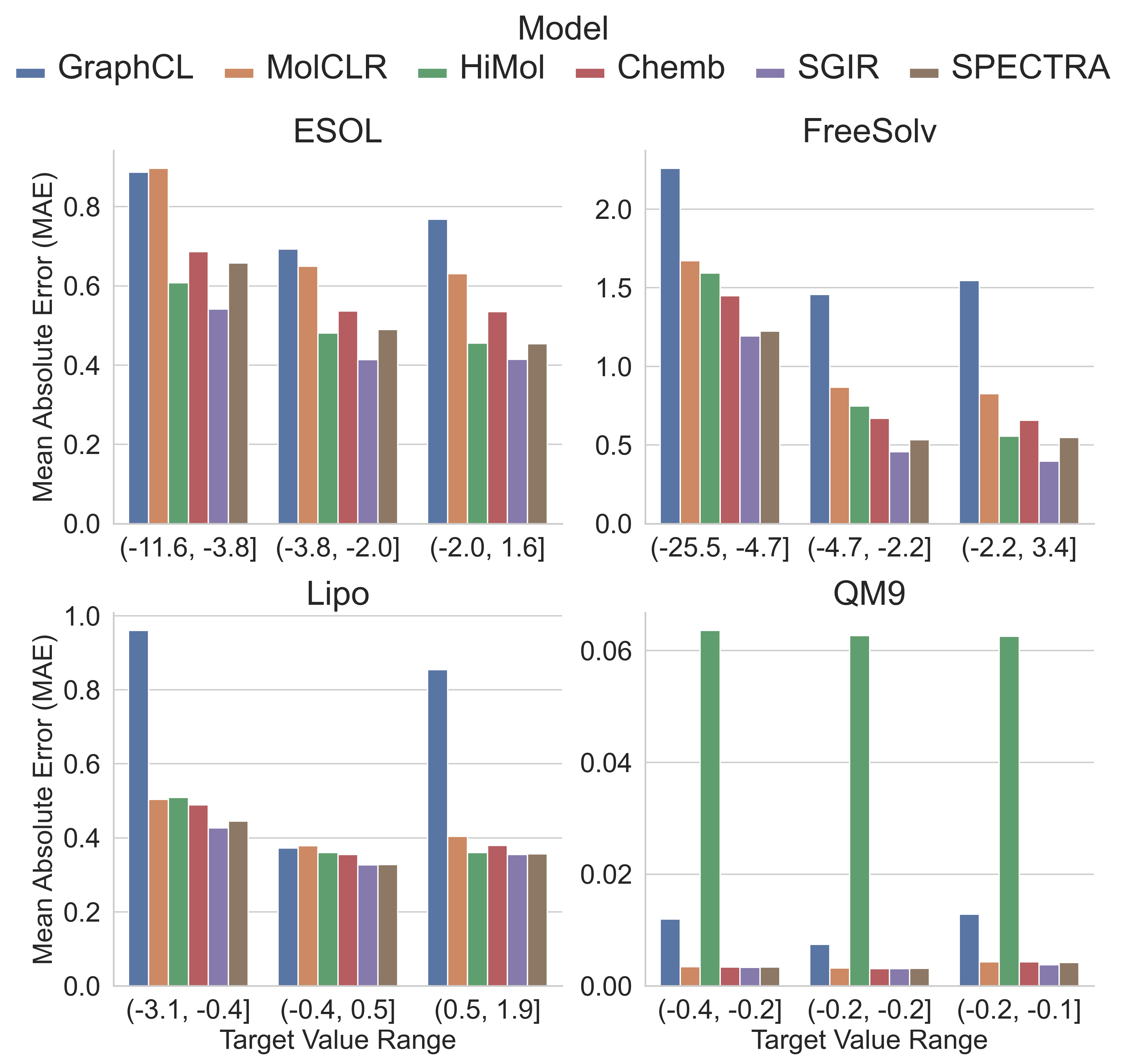
Figure 7 further dissects MAE by target value ranges. We observe that baseline models often suffer from considerably higher errors in the low-density regions, consistent with the imbalance in the training data. In contrast, SPECTRA demonstrates markedly lower errors in these sparse regions, highlighting its strength in addressing imbalance without degrading performance in high-density regions.
5. Conclusion
Experiments across benchmark datasets demonstrate that our method improves predictive accuracy in rare but critical property regimes, preserves structure–property correlations, and achieves a favorable balance between accuracy and computational efficiency. These results establish spectral-based generation as a promising and interpretable strategy for addressing class imbalance in molecular property prediction and related graph-structured scientific domains.
Several directions remain open for future work. First, we plan to extend the framework to multi-property prediction tasks and incorporate additional modalities such as 3D geometric features. Second, we aim to reduce the computational cost of Fused Gromov-Wasserstein alignment and spectral decomposition, either through more efficient algorithmic variants or hybrid strategies that combine spectral augmentation with model-based pseudo-labeling to better capture non-linear structure–label relationships. Finally, we intend to evaluate the approach on molecular datasets beyond MoleculeNet to assess generalization across domains.
6. Limitations and Ethical Considerations
For the small, drug-like molecules typical of MoleculeNet benchmarks, Fused Gromov–Wasserstein alignment remains computationally tractable. However, its cost may become prohibitive for larger and more complex graphs, such as polymers or protein–ligand systems. Addressing this limitation will require the integration of more efficient or approximate Optimal Transport solvers. In addition, our current framework is restricted to non-radical molecules, and extending it to handle radicals represents an important direction for future work
This work is intended to improve predictive modeling for scientific discovery. As with any generative augmentation method, the synthetic molecules produced should be treated as computational hypotheses subject to experimental validation, not as candidates for direct deployment. Practitioners should also be aware that imbalanced training sets often reflect real-world scarcity of certain chemical classes, and augmentation cannot substitute for domain knowledge about underrepresented regions of the chemical space.
Acknowledgements.
The project was partially supported by the National Science Foundation under the NSF Center for Computer Assisted Synthesis (C-CAS; grant no. CHE-2202693).GenAI Disclosure
We have used Generative AI in this work for English correction and code checking.
References
- (1)
- Alharbi et al. (2024) Hadeel Alharbi, Roben A Juanatas, Abdullah Al Hejaili, and Se-jung Lim. 2024. Spectral graph convolutional neural network for Alzheimer’s disease diagnosis and multi-disease categorization from functional brain changes in magnetic resonance images. Frontiers in Neuroinformatics 18 (2024), 1495571.
- Almeida et al. (2024) Rafael Lopes Almeida, Vinícius Gonçalves Maltarollo, and Frederico Gualberto Ferreira Coelho. 2024. Overcoming class imbalance in drug discovery problems: Graph neural networks and balancing approaches. Journal of Molecular Graphics and Modelling 126 (2024), 108627.
- Besharatifard and Vafaee (2024) Milad Besharatifard and Fatemeh Vafaee. 2024. A review on graph neural networks for predicting synergistic drug combinations. Artificial Intelligence Review 57, 3 (2024), 49.
- Bickerton et al. (2012) G Richard Bickerton, Gaia V Paolini, Jérémy Besnard, Sorel Muresan, and Andrew L Hopkins. 2012. Quantifying the chemical beauty of drugs. Nature chemistry 4, 2 (2012), 90–98.
- Bo et al. (2023a) Deyu Bo, Chuan Shi, Lele Wang, and Renjie Liao. 2023a. Specformer: Spectral Graph Neural Networks Meet Transformers. arXiv:2303.01028 [cs.LG] https://arxiv.org/abs/2303.01028
- Bo et al. (2023b) Deyu Bo, Xiao Wang, Yang Liu, Yuan Fang, Yawen Li, and Chuan Shi. 2023b. A survey on spectral graph neural networks. arXiv preprint arXiv:2302.05631 (2023).
- Branco et al. (2017) Paula Branco, Luís Torgo, and Rita P Ribeiro. 2017. SMOGN: a pre-processing approach for imbalanced regression. In First international workshop on learning with imbalanced domains: Theory and applications. PMLR, 36–50.
- Cao et al. (2019) Kaidi Cao, Colin Wei, Adrien Gaidon, Nikos Arechiga, and Tengyu Ma. 2019. Learning imbalanced datasets with label-distribution-aware margin loss. Advances in Neural Information Processing Systems 32 (2019).
- Chawla et al. (2002) Nitesh V Chawla, Kevin W Bowyer, Lawrence O Hall, and W Philip Kegelmeyer. 2002. SMOTE: synthetic minority over-sampling technique. Journal of artificial intelligence research 16 (2002), 321–357.
- Chen et al. (2023) Yangyang Chen, Zixu Wang, Lei Wang, Jianmin Wang, Pengyong Li, Dongsheng Cao, Xiangxiang Zeng, Xiucai Ye, and Tetsuya Sakurai. 2023. Deep generative model for drug design from protein target sequence. Journal of Cheminformatics 15, 1 (2023), 38.
- Chithrananda et al. (2020) Seyone Chithrananda, Gabriel Grand, and Bharath Ramsundar. 2020. ChemBERTa: large-scale self-supervised pretraining for molecular property prediction. arXiv preprint arXiv:2010.09885 (2020).
- Cui et al. (2019) Yin Cui, Menglin Jia, Tsung-Yi Lin, Yang Song, and Serge Belongie. 2019. Class-Balanced Loss Based on Effective Number of Samples. In Proceedings of the IEEE/CVF Conference on Computer Vision and Pattern Recognition (CVPR).
- Defferrard et al. (2016) Michaël Defferrard, Xavier Bresson, and Pierre Vandergheynst. 2016. Convolutional Neural Networks on Graphs with Fast Localized Spectral Filtering. In Advances in Neural Information Processing Systems, D. Lee, M. Sugiyama, U. Luxburg, I. Guyon, and R. Garnett (Eds.), Vol. 29. Curran Associates, Inc. https://proceedings.neurips.cc/paper_files/paper/2016/file/04df4d434d481c5bb723be1b6df1ee65-Paper.pdf
- Ding et al. (2025) Haipeng Ding, Zhewei Wei, and Yuhang Ye. 2025. Large-Scale Spectral Graph Neural Networks via Laplacian Sparsification: Technical Report. arXiv preprint arXiv:2501.04570 (2025).
- Emmert-Streib et al. (2016) Frank Emmert-Streib, Matthias Dehmer, and Yongtang Shi. 2016. Fifty years of graph matching, network alignment and network comparison. Information sciences 346-347 (2016), 180–197.
- Ertl and Schuffenhauer (2009) Peter Ertl and Ansgar Schuffenhauer. 2009. Estimation of synthetic accessibility score of drug-like molecules based on molecular complexity and fragment contributions. Journal of cheminformatics 1, 1 (2009), 8.
- Fan et al. (2024) Zhehuan Fan, Jie Yu, Xiang Zhang, Yijie Chen, Shihui Sun, Yuanyuan Zhang, Mingan Chen, Fu Xiao, Wenyong Wu, Xutong Li, et al. 2024. Reducing overconfident errors in molecular property classification using Posterior Network. Patterns 5, 6 (2024).
- Flam-Shepherd et al. (2022) Daniel Flam-Shepherd, Kevin Zhu, and Alán Aspuru-Guzik. 2022. Language models can learn complex molecular distributions. Nature Communications 13, 1 (2022), 3293.
- Gao et al. (2024) Wenhao Gao, Shitong Luo, and Connor W Coley. 2024. Generative artificial intelligence for navigating synthesizable chemical space. arXiv preprint arXiv:2410.03494 (2024).
- Giménez et al. (2010) BG Giménez, MS Santos, M Ferrarini, and JPS Fernandes. 2010. Evaluation of blockbuster drugs under the rule-of-five. Die Pharmazie-An International Journal of Pharmaceutical Sciences 65, 2 (2010), 148–152.
- Gong et al. (2022) Yu Gong, Greg Mori, and Frederick Tung. 2022. RankSim: Ranking Similarity Regularization for Deep Imbalanced Regression. arXiv:2205.15236 [cs.LG] https://arxiv.org/abs/2205.15236
- Jeon and Kim (2020) Woosung Jeon and Dongsup Kim. 2020. Autonomous molecule generation using reinforcement learning and docking to develop potential novel inhibitors. Scientific reports 10, 1 (2020), 22104.
- Jin et al. (2018) Wengong Jin, Regina Barzilay, and Tommi Jaakkola. 2018. Junction tree variational autoencoder for molecular graph generation. In International conference on machine learning. PMLR, 2323–2332.
- Karamad et al. (2020) Mohammadreza Karamad, Rishikesh Magar, Yuting Shi, Samira Siahrostami, Ian D. Gates, and Amir Barati Farimani. 2020. Orbital graph convolutional neural network for material property prediction. Phys. Rev. Mater. 4 (Sep 2020), 093801. Issue 9. doi:10.1103/PhysRevMaterials.4.093801
- Khemchandani et al. (2020) Yash Khemchandani, Stephen O’Hagan, Soumitra Samanta, Neil Swainston, Timothy J Roberts, Danushka Bollegala, and Douglas B Kell. 2020. DeepGraphMolGen, a multi-objective, computational strategy for generating molecules with desirable properties: a graph convolution and reinforcement learning approach. Journal of cheminformatics 12, 1 (2020), 53.
- Lázaro et al. (2025) Teresa Lázaro, Roger Guimerà, and Marta Sales-Pardo. 2025. Probabilistic alignment of multiple networks. Nature Communications 16, 3949 (2025).
- Lee and Min (2022) Myeonghun Lee and Kyoungmin Min. 2022. MGCVAE: multi-objective inverse design via molecular graph conditional variational autoencoder. Journal of chemical information and modeling 62, 12 (2022), 2943–2950.
- Li et al. (2024) Bowen Li, Zhen Wang, Ziqi Liu, Yanxin Tao, Chulin Sha, Min He, and Xiaolin Li. 2024. DrugMetric: quantitative drug-likeness scoring based on chemical space distance. Briefings in Bioinformatics 25, 4 (2024).
- Lim et al. (2019) Jaechang Lim, Seongok Ryu, Kyubyong Park, Yo Joong Choe, Jiyeon Ham, and Woo Youn Kim. 2019. Predicting drug–target interaction using a novel graph neural network with 3D structure-embedded graph representation. Journal of chemical information and modeling 59, 9 (2019), 3981–3988.
- Lin et al. (2017) Tsung-Yi Lin, Priya Goyal, Ross Girshick, Kaiming He, and Piotr Dollár. 2017. Focal loss for dense object detection. In Proceedings of the IEEE international conference on computer vision. 2980–2988.
- Liu et al. (2023) Gang Liu, Tong Zhao, Eric Inae, Tengfei Luo, and Meng Jiang. 2023. Semi-Supervised Graph Imbalanced Regression. In Proceedings of the 29th ACM SIGKDD Conference on Knowledge Discovery and Data Mining (Long Beach, CA, USA) (KDD ’23). Association for Computing Machinery, New York, NY, USA, 1453–1465. doi:10.1145/3580305.3599497
- Ma et al. (2025) Yihong Ma, Yijun Tian, Nuno Moniz, and Nitesh V. Chawla. 2025. Class-Imbalanced Learning on Graphs: A Survey. ACM Comput. Surv. 57, 8, Article 207 (March 2025), 16 pages. doi:10.1145/3718734
- Magar et al. (2022) Rishikesh Magar, Yuyang Wang, Cooper Lorsung, Chen Liang, Hariharan Ramasubramanian, Peiyuan Li, and Amir Barati Farimani. 2022. AugLiChem: data augmentation library of chemical structures for machine learning. Machine Learning: Science and Technology 3, 4 (nov 2022), 045015. doi:10.1088/2632-2153/ac9c84
- Marchan et al. (2025) Gabriela C Theis Marchan, Pegah Naghshnejad, Andrew Okafor, and José A Romagnoli. 2025. VAE-Assisted Data Augmentation for Improved Molecular Prediction with Graph Neural Networks (GNNs) in Low-Data Regimes. Chemical Engineering Transactions 117 (2025), 1021–1026.
- Mémoli (2011) Facundo Mémoli. 2011. Gromov–Wasserstein distances and the metric approach to object matching. Foundations of computational mathematics 11, 4 (2011), 417–487.
- Menon et al. (2020) Aditya Krishna Menon, Sadeep Jayasumana, Ankit Singh Rawat, Himanshu Jain, Andreas Veit, and Sanjiv Kumar. 2020. Long-tail learning via logit adjustment. CoRR abs/2007.07314 (2020). arXiv:2007.07314 https://arxiv.org/abs/2007.07314
- Prykhodko et al. (2019) Oleksii Prykhodko, Simon Viet Johansson, Panagiotis-Christos Kotsias, Josep Arús-Pous, Esben Jannik Bjerrum, Ola Engkvist, and Hongming Chen. 2019. A de novo molecular generation method using latent vector based generative adversarial network. Journal of cheminformatics 11, 1 (2019), 74.
- Ren et al. (2022) Jiawei Ren, Mingyuan Zhang, Cunjun Yu, and Ziwei Liu. 2022. Balanced MSE for Imbalanced Visual Regression. In Proceedings of the IEEE/CVF Conference on Computer Vision and Pattern Recognition (CVPR). 7926–7935.
- Ribeiro and Moniz (2020a) Rita P. Ribeiro and Nuno Moniz. 2020a. Imbalanced regression and extreme value prediction. Machine Learning 109, 9 (2020), 1803–1835.
- Ribeiro and Moniz (2020b) Rita P. Ribeiro and Nuno Moniz. 2020b. Imbalanced regression and extreme value prediction. Machine Learning 109, 9 (Sept. 2020), 1803–1835. doi:10.1007/s10994-020-05900-9
- Rogers and Hahn (2010) David Rogers and Mathew Hahn. 2010. Extended-connectivity fingerprints. Journal of chemical information and modeling 50, 5 (2010), 742–754.
- Ross et al. (2022) Jerret Ross, Brian Belgodere, Vijil Chenthamarakshan, Inkit Padhi, Youssef Mroueh, and Payel Das. 2022. Large-scale chemical language representations capture molecular structure and properties. Nature Machine Intelligence 4, 12 (2022), 1256–1264.
- Tian et al. (2020) Junjiao Tian, Yen-Cheng Liu, Nathaniel Glaser, Yen-Chang Hsu, and Zsolt Kira. 2020. Posterior re-calibration for imbalanced datasets. Advances in Neural Information Processing Systems 33 (2020), 8101–8113.
- Vamathevan et al. (2019) Jessica Vamathevan, Dominic Clark, Paul Czodrowski, Ian Dunham, Edgardo Ferran, George Lee, Bin Li, Anant Madabhushi, Parantu Shah, Michaela Spitzer, et al. 2019. Applications of machine learning in drug discovery and development. Nature reviews Drug discovery 18, 6 (2019), 463–477.
- Vayer et al. (2020) Titouan Vayer, Laetitia Chapel, Rémi Flamary, Romain Tavenard, and Nicolas Courty. 2020. Fused Gromov-Wasserstein distance for structured objects. Algorithms 13, 9 (2020), 212.
- Vignac et al. (2022) Clement Vignac, Igor Krawczuk, Antoine Siraudin, Bohan Wang, Volkan Cevher, and Pascal Frossard. 2022. Digress: Discrete denoising diffusion for graph generation. arXiv preprint arXiv:2209.14734 (2022).
- Wang and Zhang (2022) Xiyuan Wang and Muhan Zhang. 2022. How powerful are spectral graph neural networks. In International conference on machine learning. PMLR, 23341–23362.
- Wang et al. (2022) Yuyang Wang, Jianren Wang, Zhonglin Cao, and Amir Barati Farimani. 2022. Molecular contrastive learning of representations via graph neural networks. Nature Machine Intelligence 4, 3 (2022), 279–287.
- Wildman and Crippen (1999) Scott A Wildman and Gordon M Crippen. 1999. Prediction of physicochemical parameters by atomic contributions. Journal of chemical information and computer sciences 39, 5 (1999), 868–873.
- Wu et al. (2018) Zhenqin Wu, Bharath Ramsundar, Evan N Feinberg, Joseph Gomes, Caleb Geniesse, Aneesh S Pappu, Karl Leswing, and Vijay Pande. 2018. MoleculeNet: a benchmark for molecular machine learning. Chemical science 9, 2 (2018), 513–530.
- Xia et al. (2024) Riting Xia, Chunxu Zhang, Yan Zhang, Xueyan Liu, and Bo Yang. 2024. A novel graph oversampling framework for node classification in class-imbalanced graphs. Science China Information Sciences 67, 6 (2024), 162101.
- Xiong et al. (2019) Zhaoping Xiong, Dingyan Wang, Xiaohong Liu, Feisheng Zhong, Xiaozhe Wan, Xutong Li, Zhaojun Li, Xiaomin Luo, Kaixian Chen, Hualiang Jiang, et al. 2019. Pushing the boundaries of molecular representation for drug discovery with the graph attention mechanism. Journal of medicinal chemistry 63, 16 (2019), 8749–8760.
- Xu et al. (2022) Minkai Xu, Lantao Yu, Yang Song, Chence Shi, Stefano Ermon, and Jian Tang. 2022. Geodiff: A geometric diffusion model for molecular conformation generation. arXiv preprint arXiv:2203.02923 (2022).
- Yang et al. (2024) Kaiqi Yang, Haoyu Han, Wei Jin, and Hui Liu. 2024. Spectral-Aware Augmentation for Enhanced Graph Representation Learning. In Proceedings of the 33rd ACM International Conference on Information and Knowledge Management (Boise, ID, USA) (CIKM ’24). Association for Computing Machinery, New York, NY, USA, 2837–2847. doi:10.1145/3627673.3679762
- Yang et al. (2021) Yuzhe Yang, Kaiwen Zha, Yingcong Chen, Hao Wang, and Dina Katabi. 2021. Delving into Deep Imbalanced Regression. In Proceedings of the 38th International Conference on Machine Learning (Proceedings of Machine Learning Research, Vol. 139), Marina Meila and Tong Zhang (Eds.). PMLR, 11842–11851. https://proceedings.mlr.press/v139/yang21m.html
- Yao et al. (2024) Rufan Yao, Zhenhua Shen, Xinyi Xu, Guixia Ling, Rongwu Xiang, Tingyan Song, Fei Zhai, and Yuxuan Zhai. 2024. Knowledge mapping of graph neural networks for drug discovery: a bibliometric and visualized analysis. Frontiers in Pharmacology 15 (2024), 1393415.
- You et al. (2020) Yuning You, Tianlong Chen, Yongduo Sui, Ting Chen, Zhangyang Wang, and Yang Shen. 2020. Graph Contrastive Learning with Augmentations. In Advances in Neural Information Processing Systems, H. Larochelle, M. Ranzato, R. Hadsell, M.F. Balcan, and H. Lin (Eds.), Vol. 33. Curran Associates, Inc., 5812–5823. https://proceedings.neurips.cc/paper_files/paper/2020/file/3fe230348e9a12c13120749e3f9fa4cd-Paper.pdf
- Zang et al. (2023) Xuan Zang, Xianbing Zhao, and Buzhou Tang. 2023. Hierarchical molecular graph self-supervised learning for property prediction. Communications Chemistry 6, 1 (2023), 34.
- Zhang et al. (2023) Mengchun Zhang, Maryam Qamar, Taegoo Kang, Yuna Jung, Chenshuang Zhang, Sung-Ho Bae, and Chaoning Zhang. 2023. A survey on graph diffusion models: Generative ai in science for molecule, protein and material. arXiv preprint arXiv:2304.01565 (2023).
- Zhang et al. (2019) Si Zhang, Hanghang Tong, Jiejun Xu, and Ross Maciejewski. 2019. Graph convolutional networks: a comprehensive review. Computational Social Networks 6, 1 (2019), 1–23.
- Zhang et al. (2025) Yupu Zhang, Zelin Xu, Tingsong Xiao, Gustavo Seabra, Yanjun Li, Chenglong Li, and Zhe Jiang. 2025. DecoyDB: A Dataset for Graph Contrastive Learning in Protein-Ligand Binding Affinity Prediction. arXiv:2507.06366 [cs.LG] https://arxiv.org/abs/2507.06366
- Zong et al. (2024) Nannan Zong, Songzhi Su, and Changle Zhou. 2024. Boosting semi-supervised learning under imbalanced regression via pseudo-labeling. Concurrency and Computation: Practice and Experience 36, 19 (2024), e8103.
Appendix A Dataset Details
Our experimental evaluation uses molecular regression tasks from MoleculeNet (Wu et al., 2018), specifically ESOL, FreeSolv, Lipophilicity (Lipo) and QM9. A brief summary of these datasets is provided in Table 5. The QM9 dataset provides 12 quantum-chemical properties, from which we selected the HOMO energy as the target for evaluation.
| Dataset | # of Compounds | Description |
| ESOL | 1,128 | Water solubility (log solubility in mol/L) |
| FreeSolv | 642 | Hydration free energy in water |
| Lipophilicity | 4,200 | Octanol/water distribution coefficient (logD at pH 7.4) |
| QM9 | 133,886 | Geometric, energetic, electronic and thermodynamic |
| properties of DFT-modelled small molecules. |
Appendix B Parameter Evaluation
Figure 8 presents the impact of different value combinations of parameters in the validation sets, exploring the joint effects of the alignment parameter (which controls the balance of structural features) and the mixing coefficient . The heatmap summarizes the corresponding mean absolute error (MAE) across combinations of , allowing visual inspection of how these parameters interact and influence predictive performance. We choose lower values for as we want to be closer to the sample chosen for augmentation.

Appendix C Statistical Improvement
Table 6 provides a detailed statistical comparison between SPECTRA and all baseline models across the ESOL, FreeSolv, Lipo, and QM9 datasets. For each pairwise comparison, we compute the raw absolute-error improvement, defined as the per-sample difference in absolute prediction errors between SPECTRA and the competing model. Positive values indicate that SPECTRA produces lower predictive error. To assess whether these differences are statistically meaningful, we apply the paired t-test. The “Best Model” column identifies which method achieves the lowest absolute errors on average, while the “Significant” column reports whether the observed improvement is statistically significant.
| Dataset | Model | t-test | Mean Improvement | Best Model | Significant | |
| 0 | esol | Cheb | 0.000031 | 0.051921 | SPECTRA | Yes |
| 1 | esol | GraphCL | 0.000000 | 0.248316 | SPECTRA | Yes |
| 2 | esol | HiMol | 0.212130 | -0.019109 | HiMol | No |
| 3 | esol | MolCLR | 0.000000 | 0.191656 | SPECTRA | Yes |
| 4 | esol | Molformer | 0.000000 | 1.123755 | SPECTRA | Yes |
| 5 | esol | SGIR | 0.000000 | -0.077233 | SGIR | Yes |
| 6 | freesolv | Cheb | 0.000000 | 0.157728 | SPECTRA | Yes |
| 7 | freesolv | GraphCL | 0.000000 | 0.987215 | SPECTRA | Yes |
| 8 | freesolv | HiMol | 0.000002 | 0.197025 | SPECTRA | Yes |
| 9 | freesolv | MolCLR | 0.000000 | 0.353207 | SPECTRA | Yes |
| 10 | freesolv | Molformer | 0.000000 | 2.073809 | SPECTRA | Yes |
| 11 | freesolv | SGIR | 0.034940 | -0.085648 | SGIR | Yes |
| 12 | qm9 | Cheb | 0.000000 | 0.000037 | SPECTRA | Yes |
| 13 | qm9 | GraphCL | 0.000000 | 0.007201 | SPECTRA | Yes |
| 14 | qm9 | HiMol | 0.000000 | 0.059398 | SPECTRA | Yes |
| 15 | qm9 | MolCLR | 0.000009 | 0.000077 | SPECTRA | Yes |
| 16 | qm9 | Molformer | 0.000000 | 0.012717 | SPECTRA | Yes |
| 17 | qm9 | SGIR | 0.000000 | -0.000161 | SGIR | Yes |
| 18 | lipo | Cheb | 0.000000 | 0.031565 | SPECTRA | Yes |
| 19 | lipo | GraphCL | 0.000000 | 0.352521 | SPECTRA | Yes |
| 20 | lipo | HiMol | 0.000000 | 0.033232 | SPECTRA | Yes |
| 21 | lipo | MolCLR | 0.000000 | 0.052444 | SPECTRA | Yes |
| 22 | lipo | Molformer | 0.000000 | 0.430608 | SPECTRA | Yes |
| 23 | lipo | SGIR | 0.153037 | -0.006892 | SGIR | No |
Overall, the results demonstrate that SPECTRA consistently outperforms most baselines, with particularly strong margins on FreeSolv, showing both large error reductions and highly significant -values. A few cases, such as HiMol and SGIR on specific datasets, show either negligible differences or slight advantages for the baseline, and these are reflected accordingly in the statistical tests.
| Model | MAE (mean var) | SERA (mean var) | ||||||
| ESOL | FreeSolv | Lipo | QM9 | ESOL | FreeSolv | Lipo | QM9 | |
| ChemBERTa | 0.79 0.53 | 1.19 2.54 | 0.49 0.20 | 0.00492 0.0000 | 0.47 0.00 | 2.72 2.34 | 0.17 0.00 | 0.00003 0.0000 |
| ChemBERTa + SPECTRA | 0.80 0.50 | 1.24 2.58 | 0.49 0.20 | 0.00512 0.0000 | 0.48 0.00 | 2.80 2.23 | 0.17 0.00 | 0.00003 0.0000 |
| GCN | 0.59 0.31 | 0.81 1.05 | 0.42 0.15 | 0.00443 0.0000 | 0.24 0.00 | 0.90 0.20 | 0.12 0.00 | 0.00002 0.0000 |
| GCN + SPECTRA | 0.55 0.28 | 0.83 1.30 | 0.41 0.15 | 0.00449 0.0000 | 0.23 0.00 | 1.10 0.29 | 0.11 0.00 | 0.00002 0.0000 |
| Cheb | 0.59 0.32 | 0.93 1.26 | 0.41 0.15 | 0.00360 0.0000 | 0.25 0.01 | 1.07 0.19 | 0.11 0.00 | 0.00002 0.0000 |
| Cheb + SPECTRA (Ours) | 0.53 0.28 | 0.77 1.05 | 0.38 0.13 | 0.00357 0.0000 | 0.20 0.00 | 0.95 0.29 | 0.09 0.00 | 0.00002 0.0000 |

Appendix D Experimental Setup
All experiments were conducted on a Linux server equipped with two 12-core Intel(R) Haswell processors, 256 GB of RAM, and four NVIDIA A100 GPUs, each with 80 GB of memory. Our method is implemented in Python 3.8.19 using PyTorch 2.1.2. We used Chebyshev GCN (cheb) (Defferrard et al., 2016). We perform a manual hyperparameter search over the following ranges:
-
•
Hidden dimension:
-
•
Number of spectral block layers:
-
•
Dropout:
-
•
Learning rate:
-
•
Chebyshev filter order ():
-
•
Epochs:
-
•
Batch size:
-
•
Gamma:
-
•
Alpha:
-
•
Augmentation Percentage(%):
The optimal configuration uses a hidden dimension of 128, four layers, a dropout rate of 0.1, a learning rate of , and hyperparameters , , and . The selected augmentation rates are 0.25 for FreeSolv and 0.10 for ESOL, Lipo and QM9.
Appendix E SPECTRA Across Prediction Models
To investigate how SPECTRA-generated molecular graphs improve the performance of different prediction models, we conduct additional experiments combining SPECTRA-based augmentation with three downstream predictors: Cheb (Defferrard et al., 2016), GCN (Zhang et al., 2019), and ChemBERTa (Chithrananda et al., 2020). As shown in Table 7, the effect of SPECTRA augmentation varies across models. For GCN, SPECTRA improves performance on ESOL and Lipo. For ChemBERTa, however, the augmentation does not yield consistent gains, with slight degradation observed across several datasets — suggesting that transformer-based models pretrained on large corpora may be less sensitive to graph-level augmentation. ChebNet, on the other hand, benefits most consistently and substantially from SPECTRA augmentation, achieving the lowest MAE and SERA values across nearly all datasets. These results demonstrate that SPECTRA is broadly applicable as an augmentation strategy, while also revealing that the choice of downstream predictor plays an important role in the magnitude of improvement. The consistent superior gains observed with ChebNet across all evaluated datasets justify our design choice.
Appendix F VAE Baseline
To understand the effectiveness of our generative method, we construct a VAE baseline (Marchan et al., 2025) designed as a controlled ablation. The baseline mirrors our augmentation pipeline in every respect except the generation step: it uses the same augmentation budget, the same KDE inverse-density weighting to focus generation on underrepresented label regions, and the same five-fold cross-validation splits. In the VAE baseline, each training molecule is first encoded into a Gaussian posterior in a SELFIES-based latent space, and new samples are generated by perturbing its posterior mean with Gaussian noise before being decoded back into valid molecular structures.
Appendix G Linear Interpolation Assumption Analysis
Our augmentation method assigns property labels to generated molecules via linear interpolation. To empirically validate this assumption, we train the same Cheb model (Section 3.7) on each training fold and use it to predict properties for all augmented molecules, comparing these predictions with the interpolated labels. Figure 9 reports the mean absolute error (MAE) between and , along with the Wasserstein distance between each label distribution and the original training distribution. We observe higher MAE values for FreeSolv and Lipo, indicating larger discrepancies between interpolated and model-predicted labels, whereas ESOL and QM9 exhibit lower MAE. In terms of distributional alignment, the GNN predictions tend to more closely match the training distribution than SPECTRA (except in QM9), particularly for Lipo. However, despite the higher MAE in FreeSolv, both SPECTRA and the GNN demonstrate alignment in underrepresented regions, a trend that is also evident in ESOL. In Lipo, our method continues to provide stronger coverage of these underrepresented regions, while the GNN follows the original training distribution.
Appendix H Valid Molecule Generation
Our method adopts an exploratory strategy in which candidate molecules are generated by interpolating between structurally similar pairs. Given that linearity is a strong assumption in molecular space, we do not expect successful interpolation for all pairs, and some degree of search is inherently required. Despite this, the method consistently identifies valid molecules across datasets, even within the vast and highly discrete chemical space. The proportion of successful interpolations varies by dataset, yielding approximately 3.2% for FreeSolv, 15.6% for ESOL, 2.8% for Lipophilicity, and 27.7% for QM9. These differences reflect the influence of dataset-specific structural properties and distributional characteristics on interpolation feasibility.