跳到论文正文
W Papers独立论文阅读器 arXiv:2511.04019 论文正文 计算阅读时间 · 0%
引用这篇论文根据当前论文元数据生成,正式投稿前建议核对。


Functional central limit theorem for Euler–Maruyama scheme with decreasing step sizes

Qiyang Pei Department of Mathematics, Faculty of Science and Technology, University of Macau, Macau S.A.R., China. yc37431@um.edu.mo, qiyangpei@gmail.com and Lihu Xu Department of Mathematics, Faculty of Science and Technology, University of Macau, Macau S.A.R., China. lihuxu@um.edu.mo
(Date: 5th December 2025)
Abstract.

We consider the Euler–Maruyama (EM) scheme of a family of dissipative stochastic differential equations (SDEs), whose step sizes η1≥η2≥η3≥⋯\eta_{1}\geq\eta_{2}\geq\eta_{3}\geq\cdots are decreasing, and prove that the EM scheme weakly converges to a subordinated Brownian motion {Ba​(t)}0≤t≤1\{B_{a(t)}\}_{0\leq t\leq 1} rather than the standard Brownian motion {Bt}0≤t≤1\{B_{t}\}_{0\leq t\leq 1}, where a​(t)a(t) is an increasing function depending on the choice of {ηk}k≥1\{\eta_{k}\}_{k\geq 1}, for instance, a​(t)=t1+αa(t)=t^{1+\alpha} if ηk=k−α\eta_{k}=k^{-\alpha}.

Compared to the EM scheme with constant step sizes, there are substantial differences as the following:

  • (i)

    the EM time series is inhomogeneous and weakly converges to the ergodic measure in a polynomial speed;

  • (ii)

    we have a special number Tn=1η1+⋯+1ηnT_{n}=\frac{1}{\eta_{1}}+\cdots+\frac{1}{\eta_{n}} which roughly measures the dependence of the EM time series;

  • (iii)

    the normalized number in the CLT is nTn\frac{n}{\sqrt{T_{n}}} rather than n\sqrt{n}, in particular, nTn∝n(1−β)/2\frac{n}{\sqrt{T_{n}}}\propto n^{(1-\beta)/2} when ηk=1kβ\eta_{k}=\frac{1}{k^{\beta}} with β∈(0,1)\beta\in(0,1);

  • (iv)

    in the critical choice ηk=1k\eta_{k}=\frac{1}{k}, we have nTn=O​(1)\frac{n}{\sqrt{T_{n}}}=O(1) and thus conjecture that the CLT and FCLT do not hold. This conjecture has been verified by simulations.

A key distinction arises between the constant and decreasing step size implementations of the EM scheme. Under a constant step size, the time series is time-homogeneous. This property allows one to use a stationary initialization, which automatically eliminates several complex terms in the subsequent proof of the CLT. Conversely, the time series generated by the EM scheme with decreasing step sizes forms an inhomogeneous Markov chain. To manage the analogous difficult terms in this case, that is, when the test function hh is Lipschitz, we must instead establish a bound for the Wasserstein-2 distance W2​(θk,Xtk)W_{2}(\theta_{k},X_{t_{k}}). This technique for handling the inhomogeneous case could be of independent interest beyond the current proof.

Key words and phrases:
Stochastic differential equation; Euler-Maruyama scheme; central limit theorem; functional central limit theorem; Wasserstein distance

1. Introduction

We consider the following stochastic differential equation (SDE),

(1.1) d​Xt=b​(Xt)​d​t+σ​d​Bt,X0=x∈ℝd,\displaystyle{\rm d}X_{t}=b(X_{t}){\rm d}t+\sigma{\rm d}B_{t},\ X_{0}=x\in\mathbb{R}^{d},

where {Bt}t≥0\{B_{t}\}_{t\geq 0} is dd-dimensional standard Brownian motion, σ\sigma is an invertible d×dd\times d matrix, and the drift b:ℝd→ℝdb:\mathbb{R}^{d}\to\mathbb{R}^{d} above is assumed to satisfy Assumption 2.1, which ensures that SDE (1.1) admits a unique strong solution and a unique invariant measure π\pi; see more details in [22, 20].

In practice, we use Euler–Maruyama (EM) scheme to numerically approximate the solution of SDE (1.1), which reads as

(1.2) θk+1=θk+ηk+1​b​(θk)+ηk+1​σ​ξk+1,θ0=x,ξk+1∼i.i.d.𝒩​(0,Id),\displaystyle\theta_{k+1}=\theta_{k}+\eta_{k+1}b(\theta_{k})+\sqrt{\eta_{k+1}}\sigma\xi_{k+1},\ \theta_{0}=x,\ \xi_{k+1}\stackrel{{\scriptstyle\text{i.i.d.}}}{{\sim}}\mathcal{N}(0,I_{d}),

where 𝒩​(0,Id)\mathcal{N}(0,I_{d}) denotes the dd-dimensional standard normal distribution, and {ηk}k≥1\{\eta_{k}\}_{k\geq 1} is a decreasing sequence satisfying η1≥η2≥⋯​ηk≥ηk+1≥⋯>0\eta_{1}\geq\eta_{2}\geq\cdots\eta_{k}\geq\eta_{k+1}\geq\cdots>0 and the assumptions in Section 2.

It is easy to see that {θk}k≥0\{\theta_{k}\}_{k\geq 0} is an inhomogeneous Markov chain. Define

(1.3) t0=0;tk=η1+⋯+ηk,k≥1,\displaystyle t_{0}=0;\quad t_{k}=\eta_{1}+\cdots+\eta_{k},\quad k\geq 1,

and define the empirical measure associated to {θk}k≥0\{\theta_{k}\}_{k\geq 0} as the following:

(1.4) Πn=1n​∑k=0n−1δθk,n≥1,\displaystyle\Pi_{n}=\frac{1}{n}\sum_{k=0}^{n-1}\delta_{\theta_{k}},\quad n\geq 1,

where δθk\delta_{\theta_{k}} is the delta measure at the point θk\theta_{k}. It has been shown in [17, Theorem 2.1] that the distribution of {θk}k≥0\{\theta_{k}\}_{k\geq 0} converges to π\pi and that the empirical measure Πn\Pi_{n} weakly converges to π\pi.

We shall prove a central limit theorem (CLT) and a functional central limit theorem (FCLT) for the EM scheme sequence {θk}k≥0\{\theta_{k}\}_{k\geq 0}, more precisely, determining

(1.5) limn→∞nTn​[Πn​(h)−π​(h)]\displaystyle\lim_{n\rightarrow\infty}\frac{n}{\sqrt{T_{n}}}[\Pi_{n}(h)-\pi(h)]

and

(1.6) limn→∞{[n​t]Tn​[Π[n​t]​(h)−π​(h)]}t∈[0,1]in​D​([0,1]),\displaystyle\lim_{n\rightarrow\infty}\left\{\frac{[nt]}{\sqrt{T_{n}}}[\Pi_{[nt]}(h)-\pi(h)]\right\}_{t\in[0,1]}\quad{\rm in}\ D([0,1]),

where

(1.7) Tn=1η1+⋯+1ηn\displaystyle T_{n}=\frac{1}{\eta_{1}}+\cdots+\frac{1}{\eta_{n}}

and hh is a Lipschitz function, [x][x] denotes the integer part of x∈ℝx\in\mathbb{R}, and D​([0,1])D([0,1]) denotes the càdlàg function space from [0,1][0,1] to ℝ\mathbb{R}.

1.1. Related work

Lu et al. [20] have established a CLT with h∈Cb2​(ℝd;ℝ)h\in C_{b}^{2}(\mathbb{R}^{d};\mathbb{R}) for the EM scheme of (1.1) whose step sizes are constant, while Dai et al. extended the result in [4] to the case with the test function h∈Lip​(ℝd;ℝ)h\in\text{{\rm Lip}}(\mathbb{R}^{d};\mathbb{R}). Lovas et al. [19] established a functional CLT for stochastic gradient Langevin dynamics (SGLD) with constant step size, which converges to a standard Brownian motion. Yu et al. [34] derived a CLT for stochastic gradient descent (SGD) with constant step size by Meyn and Tweedie’s approach [24, Theorem 17.0.1]. Li et al. [16] established CLTs for the average of the outputs of SGD and momentum SGD with decreasing step sizes. Related results on moderate deviations can be found in [4, 11, 13, 27]. Jin [15] later analyzed the backward EM scheme, obtained by replacing b​(θk)b(\theta_{k}) in (1.2) with b​(θk+1)b(\theta_{k+1}), also under constant step size, and proved a CLT.

When b​(x)=−∇U​(x)b(x)=-\nabla U(x) with UU being a potential function and σ=2​Id\sigma=\sqrt{2}I_{d} with IdI_{d} being d×dd\times d identity matrix, π\pi admits a probability density proportional to e−U​(x)e^{-U(x)} and (1.2) is called unadjusted Langevin algorithm (ULA). ULA has been widely applied in statistics and data science; see for example [5, 6]. When UU is convex outside a ball and ηk=η\eta_{k}=\eta for all kk, [21] proved that ULA converges to π\pi at a speed η1/4\eta^{1/4}. This result has been extended to tamed ULA in [18, 26].

1.2. Contributions and approach

Our main results are a CLT and a FCLT. Different from the classical CLT, our scaling number is nTn\frac{n}{\sqrt{T_{n}}} rather than n\sqrt{n}. This is because that the time series {θk}k≥0\{\theta_{k}\}_{k\geq 0} is an inhomogeneous Markov chain and more and more correlated as k→∞k\rightarrow\infty. To see this, let us take ηk=1kβ\eta_{k}=\frac{1}{k^{\beta}} with β∈[0,1]\beta\in[0,1], we have

nTn≍n(β−1)/2.\displaystyle\frac{n}{\sqrt{T_{n}}}\asymp n^{(\beta-1)/2}.

As β=0\beta=0, nTn≍n1/2\frac{n}{\sqrt{T_{n}}}\asymp n^{1/2} which is the order of time-homogeneous time series. Because the correlation of {θk}k≥0\{\theta_{k}\}_{k\geq 0} increases with respect to β\beta, the scaling number nTn\frac{n}{\sqrt{T_{n}}} of CLT decreases. As β=1\beta=1, we arrive at a critical point and conjecture that the CLT does not hold true. This has been verified by simulation below. To prove the CLT, we use the decomposition (3.4) by solving the Poisson equation (2.11), in which the term MnM_{n} is a martingale difference and Rn,0,⋯,Rn,3R_{n,0},\cdots,R_{n,3} are all negligible.

As for the FCLT, unlike the classical case, the limit of our FCLT is a Brownian motion with a time change a​(t)a(t), i.e. {Ba​(t)}t∈[0,1]\{B_{a(t)}\}_{t\in[0,1]}, where

a​(t):t∈[0,1]→ℝ+.\displaystyle a(t):t\in[0,1]\rightarrow\mathbb{R}_{+}.

The form of this a​(t)a(t) depends on the choice of step sizes {ηk}k≥1\{\eta_{k}\}_{k\geq 1}. McLeish’s classical criterion for FCLT [23, Theorem 3.2] is not applied directly. Following the same argument of proving [23, Theorem 3.2] with a little adjustment, we make a tiny generalization of this criterion, which derives our FCLT immediately.

Since the Markov chain {θk}k≥0\{\theta_{k}\}_{k\geq 0} of (1.2) is inhomogeneous, it converges to the ergodic measure polynomially rather than exponentially; see [17]. This makes the techniques based on the homogeneous Markov chain such as the stationary initialization in [12, 20] not work any more, and we have to estimate the error between θk\theta_{k} and XtkX_{t_{k}} in the Wasserstein-2 distance. By the coupling technique established in [8], we show that the Wasserstein-2 distance W2​(θk,Xtk)\text{\rm{W}}_{2}(\theta_{k},X_{t_{k}}) is bounded by ηk1/4\eta_{k}^{1/4}, which is consistent with the result in [21].

Due to the inhomogeneity of {θk}k≥0\{\theta_{k}\}_{k\geq 0} of (1.2), the methods in the recent papers [4, 19, 20] such as stationary initialization [12, 20] and the techniques based on α\alpha-mixing [19] are not applicable. More precisely, thanks to the homogeneous Markov chain, [20, 4] all applied a stationary initialization trick so that {θk}k≥0\{\theta_{k}\}_{k\geq 0} is stationary, making several terms in the decomposition (3.4) below automatically vanish, and that bounding the Wasserstein-1 error W1​(θk,Xtk)\text{\rm{W}}_{1}(\theta_{k},X_{t_{k}}) is sufficient. However, in our case, it is difficult to handle these terms and we need to bound the Wasserstein-2 error W2​(θk,Xtk)\text{\rm{W}}_{2}(\theta_{k},X_{t_{k}}). Using the stationary initialization trick, [19] applied the well developed techniques for the stationary α\alpha-mixing time series to prove a functional CLT, whose limiting distribution is the standard Brownian motion.

The second difficulty in our case arises from the Lipschitz test function family, which is much larger than the function family Cb2​(ℝd;ℝ)C_{b}^{2}(\mathbb{R}^{d};\mathbb{R}). The corresponding Poisson equation has a worse regularity, this makes bounding the error terms in the decomposition (3.4) much more involved.

1.3. Notations

For two real numbers a,ba,b, we denote a∨b≔max⁡{a,b}a\lor b\coloneqq\max\{a,b\} and define [a]≔sup{n∈ℤ:n≤a}[a]\coloneqq\sup\{n\in\mathbb{Z}:n\leq a\}. For a finite set AA, we write ♯​A\sharp A to denote its cardinality.

Let Id∈ℝd×dI_{d}\in\mathbb{R}^{d\times d} be (d×d)(d\times d)-identity matrix. For the symmetric matrices A,B∈ℝd×dA,B\in\mathbb{R}^{d\times d}, write A≲BA\lesssim B if B−AB-A is positive semi-definite. The notation |⋅||\cdot| denotes the Euclidean norm for ℝd\mathbb{R}^{d}-vectors and the Frobenius norm for matrices. We write f​(n)≍g​(n)f(n)\asymp g(n) if there are constants C1,C2>0C_{1},C_{2}>0 such that for all n≥n0n\geq n_{0}, C1​f​(n)≤g​(n)≤C2​f​(n)C_{1}f(n)\leq g(n)\leq C_{2}f(n).

For a function f:ℝd→ℝf:\mathbb{R}^{d}\to\mathbb{R} that is sufficiently smooth, we denote its gradient and Hessian at xx by ∇f​(x)∈ℝd\nabla f(x)\in\mathbb{R}^{d} and ∇2f​(x)∈ℝd×d\nabla^{2}f(x)\in\mathbb{R}^{d\times d} respectively. We denote by Cbk​(ℝd;ℝ)C_{b}^{k}(\mathbb{R}^{d};\mathbb{R}) the space of the bounded continuous functions from ℝd\mathbb{R}^{d} to ℝ\mathbb{R} whose 11-st, … ,kk-th order derivatives are all bounded continuous. Denote by

Lip(ℝd;ℝ)≔{f:ℝd→ℝ:thereissomeL>0s.t.supx≠y|f​(x)−f​(y)||x−y|≤L}\displaystyle\textbf{\rm{Lip}}(\mathbb{R}^{d};\mathbb{R})\coloneqq\left\{f:\mathbb{R}^{d}\to\mathbb{R}:{\rm there\ is\ some}\ L>0\ {\rm s.t.}\ \sup_{x\neq y}\frac{|f(x)-f(y)|}{|x-y|}\leq L\right\}

the family of Lipschitz functions. For a bounded continuous function f:ℝd→ℝf:\mathbb{R}^{d}\to\mathbb{R}, we define the uniform norm ‖f‖∞≔supx∈ℝd|f​(x)|\|f\|_{\infty}\coloneqq\sup_{x\in\mathbb{R}^{d}}|f(x)|.

If a random variable XX has distribution (or law) μ\mu, we write X∼μX\sim\mu or Law​(X)=μ\text{\rm{Law}}(X)=\mu; if two random variables XX and YY have the same law, we write X=dYX\stackrel{{\scriptstyle d}}{{=}}Y. The notation Xn⇒XX_{n}\Rightarrow X denotes that the sequence of random variables {Xn}n\{X_{n}\}_{n} converges weakly to the random variable XX. We denote by 𝒩​(μ,Σ)\mathcal{N}(\mu,\Sigma) the Gaussian distribution with mean μ\mu and covariance Σ\Sigma. For a measure π\pi and a measurable function ff defined on ℝd\mathbb{R}^{d}, we write

π​(f)=∫ℝdf​(x)​π​(d​x).\displaystyle\pi(f)=\int_{\mathbb{R}^{d}}f(x)\pi({\rm d}x).

The conditional expectation 𝔼[⋅|θk]\mathbb{E}[\cdot|\theta_{k}] is abbreviated as 𝔼k​[⋅]\mathbb{E}_{k}[\cdot]. Denote by D​([0,T])D([0,T]) the Skorohod DD–space on [0,T][0,T] for T>0T>0.

The Wasserstein-pp distance between probability measures μ\mu and ν\nu is defined as

Wp​(μ,ν)=infγ∈C​(μ,ν)[𝔼(X,Y)∼γ​|X−Y|p]1/p,\displaystyle\textbf{\rm{W}}_{p}(\mu,\nu)=\inf_{\gamma\in\textbf{C}(\mu,\nu)}[\mathbb{E}_{(X,Y)\sim\gamma}|X-Y|^{p}]^{1/p},

where C​(ν,μ)\textbf{C}(\nu,\mu) denote the set of all couplings with marginals ν\nu and μ\mu, where ν\nu and μ\mu are probability measures. The Kantorovich distance of two probability measures μ\mu and ν\nu on a metric space (S,ρ)(S,\rho) is defined by

(1.8) Wρ​(ν,μ)=infγ∈C​(ν,μ)∫ρ​(x,y)​γ​(d​x,d​y).\displaystyle\text{\rm{W}}_{\rho}(\nu,\mu)=\inf_{\gamma\in\textbf{C}(\nu,\mu)}\int\rho(x,y)\gamma({\rm d}x,{\rm d}y).

Let X,YX,Y be random variables with X∼μX\sim\mu and Y∼νY\sim\nu, we will also use the notations Wp​(X,Y)≔Wp​(μ,ν)W_{p}(X,Y)\coloneqq W_{p}(\mu,\nu) and Wρ​(X,Y)≔Wρ​(μ,ν)W_{\rho}(X,Y)\coloneqq W_{\rho}(\mu,\nu).

To study EM scheme (1.2), it will be helpful to consider the following auxiliary continuous system:

(1.9) Y0=x,d​Yt=b​(Ytk−1)​d​t+σ​d​Bt,t∈(tk−1,tk],k≥1.\displaystyle\begin{split}&Y_{0}=x,\\ &{\rm d}Y_{t}=b(Y_{t_{k-1}}){\rm d}t+\sigma{\rm d}B_{t},\ t\in(t_{k-1},t_{k}],\quad k\geq 1.\end{split}

It is easy to see that YtkY_{t_{k}} and θk\theta_{k} have the same distributions for all kk.

1.4. Organization of this paper

In the next section, we first provide the assumptions and then present the main results, Theorems 2.4 and 2.6, and the byproducts of independent interest, Theorems 2.7 and 2.8. We then provide a discussion of the results and point out that a special step sizes {1/k}k≥1\{1/k\}_{k\geq 1} may leads to a non-existence of CLT, accompanied by simulation verification. The remaining of the paper is devoted to proving the CLT and the FCLT. To this end, we establish several supporting results; see Figure 1 for a map of the proof.

Refer to caption
Figure 1. The map of proof

In Section 3, we derive the decomposition (3.4). The remainder terms Rn,0,⋯,Rn,3R_{n,0},\cdots,R_{n,3} therein are justified to be negligible (Lemma 3.4), proved by Lemmas 3.1, 3.2 and 3.3. With Lemma 3.4 in hand, it is sufficient to prove the CLT and the FCLT for the martingale part in (3.4). Lemmas in Section 3 are proved in Appendix A.

The CLT is proved in Section 4 by weak comparison (Lemma 4.1). As a byproduct, we obtain a Wasserstein-2 error bound (Theorem 2.7). Theorem 2.7 is proved in Section 6, preceded by Lemmas 6.1 and 6.2. Lemma 4.1, along with Lemmas 6.1 and 6.2, is proved in Appendix B.

The FCLT is proved in Section 5 by verifying the conditions of a criterion (Theorem 2.8). Since the criterion is a slightly modification of [23, Theorem 3.2], we include its proof in Appendix C for completeness.

2. Assumptions and Main results

2.1. Assumptions

For the drift of SDE (1.1) and EM scheme, we need the following assumptions:

Assumption 2.1.

Assume that the drift b:ℝd→ℝdb:\mathbb{R}^{d}\to\mathbb{R}^{d} of SDE (1.1) is continuous and satisfies the following conditions:
(1)(1) ((Lipschitz condition)): There exists some constant L>0L>0, such that

|b​(x)−b​(y)|≤L​|x−y|,∀x,y∈ℝd;\displaystyle|b(x)-b(y)|\leq L|x-y|,\quad\forall x,y\in\mathbb{R}^{d};

(2)(2) ((Partial dissipation)): There exist constants K1>0K_{1}>0, K2≥0K_{2}\geq 0, such that

⟨b​(x)−b​(y),x−y⟩≤−K1​|x−y|2+K2,∀x,y∈ℝd.\displaystyle\langle b(x)-b(y),x-y\rangle\leq-K_{1}|x-y|^{2}+K_{2},\quad\forall x,y\in\mathbb{R}^{d}.

Assume that there exists K3>1K_{3}>1, such that σ∈ℝd×d\sigma\in\mathbb{R}^{d\times d} of SDE (1.1) is invertible and satisfies

K3−1​Id≲σ​σ⊺≲K3​Id.\displaystyle K_{3}^{-1}I_{d}\lesssim\sigma\sigma^{\intercal}\lesssim K_{3}I_{d}.

The Assumption 2.1 implies that for some C>0C>0, for all x,y∈ℝdx,y\in\mathbb{R}^{d},

(2.1) ⟨x,b​(x)⟩\displaystyle\langle x,b(x)\rangle ≤−K12​|x|2+C,\displaystyle\leq-\frac{K_{1}}{2}|x|^{2}+C,
(2.2) |b​(x)|\displaystyle|b(x)| ≤C​(1+|x|),\displaystyle\leq C(1+|x|),

and

(2.3) K3−1​|y|2≤|σ−1​y|2≤K3​|y|2.\displaystyle K_{3}^{-1}|y|^{2}\leq|\sigma^{-1}y|^{2}\leq K_{3}|y|^{2}.

It is easy to see that the infinitesimal generator of the SDE (1.1) is

(2.4) 𝒜​f​(x)=⟨b​(x),∇f​(x)⟩+12​⟨σ​σ⊺,∇2f​(x)⟩HS,\displaystyle\mathcal{A}f(x)=\langle b(x),\nabla f(x)\rangle+\frac{1}{2}\langle\sigma\sigma^{\intercal},\nabla^{2}f(x)\rangle_{\text{HS}},

and [20, Lemma 2.3] shows that for V​(x)=1+|x|2V(x)=1+|x|^{2}, one has

(2.5) 𝒜​V​(x)≤−λ​V​(x)+q\displaystyle\mathcal{A}V(x)\leq-\lambda V(x)+q

for some constants λ,q>0\lambda,q>0.

Assumption 2.2.

The sequence of step sizes {ηk}k≥1⊂(0,1)\{\eta_{k}\}_{k\geq 1}\subset(0,1) is non-increasing and satisfies the following conditions:
(1)(1)

∑k=1∞ηk=∞.\displaystyle\sum_{k=1}^{\infty}\eta_{k}=\infty.

(2)(2) For some constant c>0c>0,

(2.6) ηk−1−ηk≤c​ηk2,k≥2.\displaystyle\eta_{k-1}-\eta_{k}\leq c\eta_{k}^{2},\quad k\geq 2.
Assumption 2.3.

The sequence of step sizes {ηk}k≥1⊂(0,1)\{\eta_{k}\}_{k\geq 1}\subset(0,1) further satisfies:
(1)(1) For some 0<ϵ<10<\epsilon<1,

(2.7) ∑k=1∞ηk2−ϵ<∞.\displaystyle\sum_{k=1}^{\infty}\eta_{k}^{2-\epsilon}<\infty.

(2)(2) As n→∞n\to\infty,

(2.8) log⁡nηn​Tn→0,\displaystyle\frac{\sqrt{\log n}}{\eta_{n}\sqrt{T_{n}}}\to 0,

where TnT_{n} is defined by (1.7).

Remark 2.1.

11. The classical Robbins and Monro condition [28] is given by:

(2.9) ∑k=1∞ηk=∞,∑k=1∞ηk2<∞.\displaystyle\sum_{k=1}^{\infty}\eta_{k}=\infty,\quad\sum_{k=1}^{\infty}\eta_{k}^{2}<\infty.

However, due to the lower regularity of the solution to Poisson equation, we require a slightly stronger condition, as stated in (1)(1) of Assumption 2.3.
22. Condition (2)(2) in Assumption 2.3 implies that for any constant C>0C>0, we have Cηn​Tn→0\frac{C}{\eta_{n}\sqrt{T_{n}}}\to 0 as n→∞n\to\infty. The term log⁡n\sqrt{\log n} appears for technical reason and is not the only possible choice; see the proof of Lemma 3.3 for details.

2.2. The main results

Consider Πn\Pi_{n} with a test function h∈Lip​(ℝd;ℝ)h\in\text{\rm{Lip}}(\mathbb{R}^{d};\mathbb{R}), i.e.

Πn​(h)=1n​∑k=0n−1δθk​(h)=1n​∑k=0n−1h​(θk).\displaystyle\Pi_{n}(h)=\frac{1}{n}\sum_{k=0}^{n-1}\delta_{\theta_{k}}(h)=\frac{1}{n}\sum_{k=0}^{n-1}h(\theta_{k}).

Under the above assumptions, we shall prove the following CLT.

Theorem 2.4.

Suppose that Assumptions 2.1, 2.2 and 2.3 hold. Assume that η1≤η∗\eta_{1}\leq\eta^{\ast} for some sufficiently small η∗>0\eta^{\ast}>0. Let h∈Lip​(ℝd;ℝ)h\in\text{\rm{Lip}}(\mathbb{R}^{d};\mathbb{R}), then we have

(2.10) nTn​[Πn​(h)−π​(h)]⇒𝒩​(0,π​(|σ⊺​∇φ|2)), as ​n→∞,\displaystyle\frac{n}{\sqrt{T_{n}}}[\Pi_{n}(h)-\pi(h)]\Rightarrow\mathcal{N}(0,\pi(|\sigma^{\intercal}\nabla\varphi|^{2})),\quad\text{ as }n\to\infty,

where φ\varphi solves Poisson equation

(2.11) h−π​(h)=𝒜​φ,\displaystyle h-\pi(h)=\mathcal{A}\varphi,

and 𝒜\mathcal{A} is the generator of SDE (1.1) given by (2.4).

Remark 2.2.

The order of n​Tn−1/2nT_{n}^{-1/2} is determined by the choice of step sizes {ηk}k≥1\{\eta_{k}\}_{k\geq 1}. In the classical CLT framework, the order of time scaling factor is n1/2n^{1/2}; see, for example, [7, Theorem 3.4.1]. In our setting, n⋅Tn−1/2n\cdot T_{n}^{-1/2} varies with {ηk}k≥1\{\eta_{k}\}_{k\geq 1}. For instance, when ηk=k−β\eta_{k}=k^{-\beta}, n​Tn−1/2nT_{n}^{-1/2} is of order n(1−β)/2n^{(1-\beta)/2}.

Furthermore, we obtain a FCLT related to Theorem 2.4 under the following extra assumption.

Assumption 2.5.

Let T>0T>0. Assume that:
(1)(1) a​(t):[0,T]→ℝ+a(t):[0,T]\to\mathbb{R}_{+} be a strictly increasing continuous function on [0,T][0,T] satisfying a​(0)=0a(0)=0;
(2)(2)For any constant C>0C>0,

limδ→0τ​(δ)δ⋅e−C​τ​(δ)−2=0,\displaystyle\lim_{\delta\to 0}\frac{\tau(\delta)}{\delta}\cdot e^{-C\tau(\delta)^{-2}}=0,

where τm​(δ)≔a​((m+1)​δ)−a​(m​δ)\tau_{m}(\delta)\coloneqq\sqrt{a((m+1)\delta)-a(m\delta)} and τ​(δ)≔supm<δ−1​Tτm​(δ)\tau(\delta)\coloneqq\sup_{m<\delta^{-1}T}\tau_{m}(\delta).

Theorem 2.6.

Under the assumptions of Theorem 2.4, assume further the limit

a​(t)≔limn→∞T[n​t]Tn∈[0,1]\displaystyle a(t)\coloneqq\lim_{n\to\infty}\frac{T_{[nt]}}{T_{n}}\in[0,1]

exists and satisfies Assumption 2.5 with T=1T=1. Then one has

{[n​t]Tn​[Π[n​t]​(h)−π​(h)]}t∈[0,1]⇒π​(|σ⊺​∇φ|2)​{Ba​(t)}t∈[0,1]\displaystyle\left\{\frac{[nt]}{\sqrt{T_{n}}}[\Pi_{[nt]}(h)-\pi(h)]\right\}_{t\in[0,1]}\Rightarrow\sqrt{\pi(|\sigma^{\intercal}\nabla\varphi|^{2})}\{B_{a(t)}\}_{t\in[0,1]}

as n→∞n\to\infty on D​([0,1])D([0,1]).

An example: Let ηk=k−α\eta_{k}=k^{-\alpha}, α∈(12−ϵ,1)\alpha\in(\frac{1}{2-\epsilon},1), T=1T=1. It is easy to check that

a​(t)=limn→∞T[n​t]Tn=t1+α,\displaystyle a(t)=\lim_{n\to\infty}\frac{T_{[nt]}}{T_{n}}=t^{1+\alpha},

which satisfies Assumption 2.5, so that Theorem 2.6 tells us

{[n​t]Tn​[Π[n​t]​(h)−π​(h)]}t∈[0,1]⇒π​(|σ⊺​∇φ|2)​{Bt1+α}t∈[0,1].\displaystyle\left\{\frac{[nt]}{\sqrt{T_{n}}}[\Pi_{[nt]}(h)-\pi(h)]\right\}_{t\in[0,1]}\Rightarrow\sqrt{\pi(|\sigma^{\intercal}\nabla\varphi|^{2})}\left\{B_{t^{1+\alpha}}\right\}_{t\in[0,1]}.

2.3. Byproducts of independent interest

When proving Theorem 2.4, we need the crucial Lemma 4.1 below, whose proof heavily depends on a bound on the Wasserstein-2 distance W2​(Xtn,θn)\text{\rm{W}}_{2}(X_{t_{n}},\theta_{n}) as the following. Such bound for W2​(Xtn,θn)\text{\rm{W}}_{2}(X_{t_{n}},\theta_{n}) is of independent interest.

Theorem 2.7.

Suppose that Assumption 2.1 and Assumption 2.2 hold. Assume that η1≤η∗\eta_{1}\leq\eta^{\ast} for some sufficiently small η∗>0\eta^{\ast}>0. Let {Xt}t≥0\{X_{t}\}_{t\geq 0} and {θk}k≥0\{\theta_{k}\}_{k\geq 0} be given as in (1.1) and (1.9) respectively. For all n≥1n\geq 1, any 0≤i<n0\leq i<n, with Xti=θi=z∈ℝdX_{t_{i}}=\theta_{i}=z\in\mathbb{R}^{d} be given, we have

W2​(Xtn,θn)≤C​(1+|z|1/2)​ηn1/4.\displaystyle\text{\rm{W}}_{2}(X_{t_{n}},\theta_{n})\leq C(1+|z|^{1/2})\eta_{n}^{1/4}.
Remark 2.3.

Majka et al [21] proved the Wasserstein-2 convergence rate for ULA with a fixed step size to the target distribution π\pi is of order η1/4\eta^{1/4}. Their approach employs a novel coupling technique that combines synchronous coupling with the coupling method introduced in [10]. [21, Section 5.1] gives a brief discussion on the possible extension to the case of decreasing step sizes.

When proving Theorem 2.6, McLeish’s classical criterion in [23, Theorem 3.2] is not applied directly. Following the argument of proving [23, Theorem 3.2], we make a tiny generalization of this criterion, which can be directly applied to prove our FCLT.

Theorem 2.8.

Let {kn​(t)}n≥1\{k_{n}(t)\}_{n\geq 1} be a sequence of integer-valued non-decreasing right-continuous function defined on [0,T][0,T] with kn​(0)=0k_{n}(0)=0 for all n≥1n\geq 1. Suppose Xn,iX_{n,i} is a martingale difference array satisfying that for each t∈[0,T]t\in[0,T], as n→∞n\to\infty:
(1)(1) maxi≤kn​(t)⁡|Xn,i|→0\max_{i\leq k_{n}(t)}|X_{n,i}|\to 0 in L2L^{2};
(2)(2) ∑i=1kn​(t)Xn,i2→a​(t)\sum_{i=1}^{k_{n}(t)}X_{n,i}^{2}\to a(t) in Probability.
Let

Bn​(t)≔∑i=1kn​(t)Xn,i,t∈[0,T].\displaystyle B_{n}(t)\coloneqq\sum_{i=1}^{k_{n}(t)}X_{n,i},\ t\in[0,T].

Then, under Assumption 2.5,

{Bn​(t)}t∈[0,T]⇒{Ba​(t)}t∈[0,T]\displaystyle\{B_{n}(t)\}_{t\in[0,T]}\Rightarrow\{B_{a(t)}\}_{t\in[0,T]}

as n→∞n\to\infty on D​([0,T])D([0,T]), where BB denotes standard Brownian motion.

Theorem 2.8 can be proved by following the argument in proving [23, Theorem 3.2]. We put its proof in Appendix C.

2.4. Discussions on a special case

Let us discuss a special step size ηk=1k\eta_{k}=\frac{1}{k} with k≥1k\geq 1, we have

1ηn​Tn≍1,\displaystyle\frac{1}{\eta_{n}\sqrt{T_{n}}}\asymp 1,

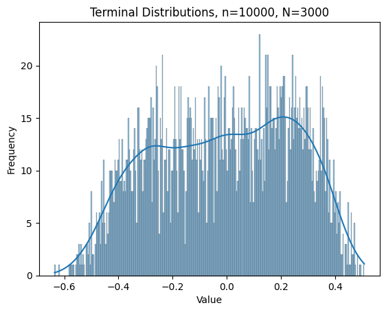
so that Assumption 2.3 is not satisfied. We conduct simulations to investigate whether the CLT fails in this case.

We consider the one dimensional case, setting σ=1\sigma=1 and choosing

b​(x)=−x+sin⁡x.\displaystyle b(x)=-x+\sin x.

Let the Lipschitz test function be

h​(x)=11+x2.\displaystyle h(x)=\frac{1}{1+x^{2}}.

We run the EM scheme N=3000N=3000 times, each with n=105n=10^{5} iterations whose initializations are uniformly chosen from {−8,2,12}\{-8,2,12\}. We consider three step size sequences:

ηk=1k3/4,ηk=log⁡(k+1)k+1,ηk=1k.\displaystyle\eta_{k}=\frac{1}{k^{3/4}},\quad\eta_{k}=\frac{\log(k+1)}{k+1},\quad\eta_{k}=\frac{1}{k}.

The first two satisfy Assumption 2.3, while the third fails.

The resulting empirical distributions of Tn−1/2​∑k=0n−1[h​(θk)−π​(h)]T_{n}^{-1/2}\sum_{k=0}^{n-1}[h(\theta_{k})-\pi(h)] are shown in Figure 2, which suggests that the CLT may not hold when Assumption 2.3 is violated.

Figure 2. Distribution of 1Tn​∑k=0n−1[h​(θk)−π​(h)]\frac{1}{\sqrt{T_{n}}}\sum_{k=0}^{n-1}[h(\theta_{k})-\pi(h)], h​(x)=11+x2h(x)=\frac{1}{1+x^{2}}, n=105n=10^{5}.
Refer to caption
(a) ηk=1k0.75\eta_{k}=\frac{1}{k^{0.75}}
Refer to caption
(b) ηk=log⁡(1+k)k+1\eta_{k}=\frac{\log(1+k)}{k+1}
Refer to caption
(c) ηk=1k\eta_{k}=\frac{1}{k}

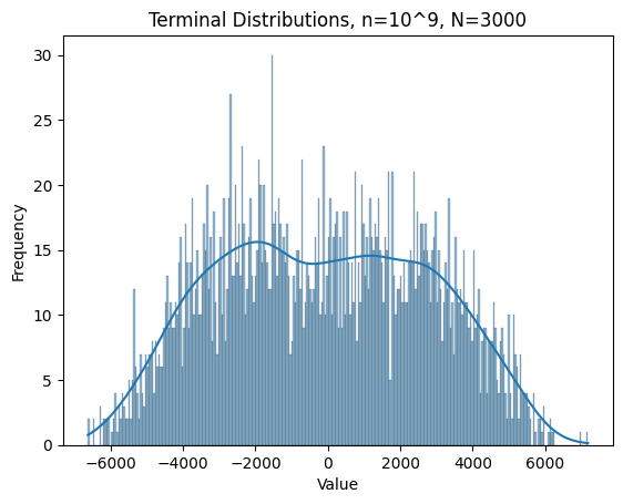
One may doubt whether such failure is due to insufficient number of iterations since ∑k=1105(1/k)≈9.7\sum_{k=1}^{10^{5}}(1/k)\approx 9.7. To test this concern, we fix the step size sequence as ηk=1/k\eta_{k}=1/k, increase the number of iterations to n=109n=10^{9} and consider three different test functions

h​(x)=11+x2,h​(x)=sin⁡x,h​(x)=x.\displaystyle h(x)=\frac{1}{1+x^{2}},\quad h(x)=\sin x,\quad h(x)=x.

The results are shown in Figure 3, which shows significant variation across different test functions, suggesting that the CLT does not hold when ηk=1/k\eta_{k}=1/k. We leave it as a problem.

Problem 2.9.

Let TnT_{n} be defined as in (1.7), and let {θk}k≥0\{\theta_{k}\}_{k\geq 0} be defined as in (1.2) under Assumption 2.1, with step sizes ηk=1/k\eta_{k}=1/k. Determine the limiting distribution of Tn−1/2​∑k=0n−1[h​(θk)−π​(h)]T_{n}^{-1/2}\sum_{k=0}^{n-1}[h(\theta_{k})-\pi(h)] as n→∞n\to\infty.

Figure 3. Distribution of 1Tn​∑k=0n−1[h​(θk)−π​(h)]\frac{1}{\sqrt{T_{n}}}\sum_{k=0}^{n-1}[h(\theta_{k})-\pi(h)], ηk=1k\eta_{k}=\frac{1}{k}, n=109n=10^{9}.
Refer to caption
(a) h​(x)=11+x2h(x)=\frac{1}{1+x^{2}}
Refer to caption
(b) h​(x)=sin⁡xh(x)=\sin x
Refer to caption
(c) h​(x)=xh(x)=x

3. Decomposition, Poisson equation and auxiliary lemmas

Let us give the strategy for proving our main results, which includes a decomposition and a Poisson equation, and auxiliary lemmas for the proofs.

3.1. The strategy for proving CLT

Let φ:ℝd→ℝ\varphi:\mathbb{R}^{d}\rightarrow\mathbb{R} be a function with a certain regularity such that the following Taylor expansion holds:

φ​(θk+1)−φ​(θk)=⟨∇φ​(θk),Δ​θk+1⟩+12​⟨∇2φ​(θk),(Δ​θk+1)​(Δ​θk+1)⊺⟩HS+ℛk+1,\displaystyle\varphi(\theta_{k+1})-\varphi(\theta_{k})=\langle\nabla\varphi(\theta_{k}),\Delta\theta_{k+1}\rangle+\frac{1}{2}\langle\nabla^{2}\varphi(\theta_{k}),(\Delta\theta_{k+1})(\Delta\theta_{k+1})^{\intercal}\rangle_{\text{HS}}+\mathcal{R}_{k+1},

where

(3.1) Δ​θk+1≔θk+1−θk=ηk+1​b​(θk)+ηk+1​σ​ξk+1,\displaystyle\Delta\theta_{k+1}\coloneqq\theta_{k+1}-\theta_{k}=\eta_{k+1}b(\theta_{k})+\sqrt{\eta_{k+1}}\sigma\xi_{k+1},
(3.2) ℛk+1≔∫01∫01r​⟨∇2φ​(θk+r​s​Δ​θk+1)−∇2φ​(θk),(Δ​θk+1)​(Δ​θk+1)⊺⟩HS​dr​ds.\displaystyle\mathcal{R}_{k+1}\coloneqq\int_{0}^{1}\int_{0}^{1}r\langle\nabla^{2}\varphi(\theta_{k}+rs\Delta\theta_{k+1})-\nabla^{2}\varphi(\theta_{k}),(\Delta\theta_{k+1})(\Delta\theta_{k+1})^{\intercal}\rangle_{\text{HS}}{\rm d}r{\rm d}s.

Recall the definition of 𝒜\mathcal{A} from (2.4), we have

(3.3) φ​(θk+1)−φ​(θk)−ηk+1​𝒜​φ​(θk)=ηk+1​⟨∇φ​(θk),σ​ξk+1⟩+12​⟨∇2φ​(θk),(Δ​θk+1)​(Δ​θk+1)⊺−ηk+1​σ​σ⊺⟩HS+ℛk+1.\displaystyle\begin{split}&\varphi(\theta_{k+1})-\varphi(\theta_{k})-\eta_{k+1}\mathcal{A}\varphi(\theta_{k})\\ =&\sqrt{\eta_{k+1}}\langle\nabla\varphi(\theta_{k}),\sigma\xi_{k+1}\rangle+\frac{1}{2}\langle\nabla^{2}\varphi(\theta_{k}),(\Delta\theta_{k+1})(\Delta\theta_{k+1})^{\intercal}-\eta_{k+1}\sigma\sigma^{\intercal}\rangle_{\text{HS}}+\mathcal{R}_{k+1}.\end{split}

In order to make a connection between the above expansion and our CLT, we introduce the Poisson equation (2.11), i.e.,

𝒜​φ=h−π​(h).\displaystyle\mathcal{A}\varphi=h-\pi(h).

Let φ\varphi be the solution to the Poisson equation, we obtain:

∑k=0n−1[h​(θk)−π​(h)]\displaystyle\sum_{k=0}^{n-1}[h(\theta_{k})-\pi(h)] =∑k=0n−11ηk+1​𝒜​φ​(θk)​ηk+1\displaystyle=\sum_{k=0}^{n-1}\frac{1}{\eta_{k+1}}\mathcal{A}\varphi(\theta_{k})\eta_{k+1}
=∑k=0n−11ηk+1​[𝒜​φ​(θk)​ηk+1−[φ​(θk+1)−φ​(θk)]]+∑k=0n−1φ​(θk+1)−φ​(θk)ηk+1.\displaystyle=\sum_{k=0}^{n-1}\frac{1}{\eta_{k+1}}\left[\mathcal{A}\varphi(\theta_{k})\eta_{k+1}-[\varphi(\theta_{k+1})-\varphi(\theta_{k})]\right]+\sum_{k=0}^{n-1}\frac{\varphi(\theta_{k+1})-\varphi(\theta_{k})}{\eta_{k+1}}.

By (3.3), we further get the following decomposition:

(3.4) 1Tn​∑k=0n−1[h​(θk)−π​(h)]=1Tn​Mn+Rn,0+Rn,1−Rn,2−Rn,3,\displaystyle\frac{1}{\sqrt{T_{n}}}\sum_{k=0}^{n-1}[h(\theta_{k})-\pi(h)]=\frac{1}{\sqrt{T_{n}}}M_{n}+R_{n,0}+R_{n,1}-R_{n,2}-R_{n,3},

where

Mn≔\displaystyle M_{n}\coloneqq −∑k=0n−11ηk+1​⟨∇φ​(θk),σ​ξk+1⟩,\displaystyle-\sum_{k=0}^{n-1}\frac{1}{\sqrt{\eta_{k+1}}}\langle\nabla\varphi(\theta_{k}),\sigma\xi_{k+1}\rangle,
Rn,0≔\displaystyle R_{n,0}\coloneqq 1Tn​∑k=0n−11ηk+1​[φ​(θk+1)−φ​(θk)],\displaystyle\frac{1}{\sqrt{T_{n}}}\sum_{k=0}^{n-1}\frac{1}{\eta_{k+1}}[\varphi(\theta_{k+1})-\varphi(\theta_{k})],
Rn,1≔\displaystyle R_{n,1}\coloneqq 12​Tn​∑k=0n−1⟨∇2φ​(θk),σ​σ⊺−(σ​ξk+1)​(σ​ξk+1)⊺⟩HS\displaystyle\frac{1}{2\sqrt{T_{n}}}\sum_{k=0}^{n-1}\langle\nabla^{2}\varphi(\theta_{k}),\sigma\sigma^{\intercal}-(\sigma\xi_{k+1})(\sigma\xi_{k+1})^{\intercal}\rangle_{\text{HS}}
+12​Tn​∑k=0n−1ηk+11/2​⟨∇2φ​(θk),b​(θk)​(σ​ξk+1)⊺+(σ​ξk+1)​b​(θk)⊺⟩HS,\displaystyle+\frac{1}{2\sqrt{T_{n}}}\sum_{k=0}^{n-1}\eta_{k+1}^{1/2}\langle\nabla^{2}\varphi(\theta_{k}),b(\theta_{k})(\sigma\xi_{k+1})^{\intercal}+(\sigma\xi_{k+1})b(\theta_{k})^{\intercal}\rangle_{\text{HS}},
Rn,2≔\displaystyle R_{n,2}\coloneqq 12​Tn​∑k=0n−1ηk+1​⟨∇2φ​(θk),b​(θk)​b​(θk)⊺⟩HS,\displaystyle\frac{1}{2\sqrt{T_{n}}}\sum_{k=0}^{n-1}\eta_{k+1}\langle\nabla^{2}\varphi(\theta_{k}),b(\theta_{k})b(\theta_{k})^{\intercal}\rangle_{\text{HS}},
Rn,3≔\displaystyle R_{n,3}\coloneqq 1Tn​∑k=0n−11ηk+1​ℛk+1.\displaystyle\frac{1}{\sqrt{T_{n}}}\sum_{k=0}^{n-1}\frac{1}{\eta_{k+1}}\mathcal{R}_{k+1}.

With the decomposition (3.4), we shall apply CLT criterion for martingale difference sequence to handle Tn−1/2​MnT_{n}^{-1/2}M_{n} and prove that the remainder terms Rn,0,…,Rn,3R_{n,0},...,R_{n,3} are all negligible.

To advance this strategy, we require the following auxiliary lemmas, which encompass the regularity of the Poisson equation, the moment estimates associated with SDE and the bounds with respect to step sizes.

3.2. Poisson equation (2.11) and regularity of its solution

Let φ\varphi be the solution of Poisson equation (2.11), namely:

𝒜​φ=h−π​(h).\displaystyle\mathcal{A}\varphi=h-\pi(h).

When the test function h∈Cb2​(ℝd;ℝ)h\in C_{b}^{2}(\mathbb{R}^{d};\mathbb{R}), it follows that the solution φ∈Cb4\varphi\in C_{b}^{4} with ‖∇kφ‖∞≤C\|\nabla^{k}\varphi\|_{\infty}\leq C, k=0,1,2,3,4k=0,1,2,3,4, as shown in [20, Lemma 3.1]. In this paper, we consider test function h∈Lip​(ℝd;ℝ)h\in\text{\rm{Lip}}(\mathbb{R}^{d};\mathbb{R}) for instead, and the corresponding regularity of φ\varphi is given by the following lemma.

Lemma 3.1 (Lemma 3.3 in [4]).

Let the Assumption 2.1 hold. Let h∈Lip​(ℝd;ℝ)h\in\text{\rm{Lip}}(\mathbb{R}^{d};\mathbb{R}), and let φ\varphi be solution to Poisson equation (2.11). Then there exists a constant C>0C>0, such that

(3.5) |∇kφ​(x)|≤C​(1+|x|k+2),k=0,1,2.\displaystyle|\nabla^{k}\varphi(x)|\leq C(1+|x|^{k+2}),\ k=0,1,2.

Further, it follows that

(3.6) supy:|y−x|≤1|∇2φ​(x)−∇2φ​(y)||x−y|≤C​(1+|x|5).\displaystyle\sup_{y:|y-x|\leq 1}\frac{|\nabla^{2}\varphi(x)-\nabla^{2}\varphi(y)|}{|x-y|}\leq C(1+|x|^{5}).

3.3. Remainder terms in decomposition (3.4) are negligible

Since each remainder term involves both sequences {θk}k≥0\{\theta_{k}\}_{k\geq 0} and {ηk}k≥1\{\eta_{k}\}_{k\geq 1}, we additionally introduce two auxiliary lemmas to address their respective properties; see Appendix A for their proofs.

Lemma 3.2 (Moment estimations).

Let {Xt}t≥0\{X_{t}\}_{t\geq 0} be the solution of SDE (1.1), and {θk}k≥1\{\theta_{k}\}_{k\geq 1} be the associated EM scheme defined by (1.2) Then, under the Assumption 2.1, one has:
(1)(1) For any p≥1p\geq 1, there exist a positive constant C1>0C_{1}>0 such that

supt≥s𝔼​[|Xt|p|Xs=z]≤C1​(1+|z|p)\displaystyle\sup_{t\geq s}\mathbb{E}[|X_{t}|^{p}|X_{s}=z]\leq C_{1}(1+|z|^{p})

for all s≥0s\geq 0 and z∈ℝdz\in\mathbb{R}^{d}.
(2)(2) Let Assumption 2.2 hold. Assume further that there exists η∗>0\eta^{\ast}>0 sufficiently small, such that η1<η∗\eta_{1}<\eta^{\ast}. Then for any p≥1p\geq 1, there exists a positive constant C2>0C_{2}>0 such that

(3.7) supk≥i𝔼​[|b​(θk)|p|θi=z]≤C2​(1+|z|p),supk≥i𝔼​[|θk|p|θi=z]≤C2​(1+|z|p)\displaystyle\sup_{k\geq i}\mathbb{E}[|b(\theta_{k})|^{p}|\theta_{i}=z]\leq C_{2}(1+|z|^{p}),\quad\sup_{k\geq i}\mathbb{E}[|\theta_{k}|^{p}|\theta_{i}=z]\leq C_{2}(1+|z|^{p})

for all i≥0i\geq 0 and z∈ℝdz\in\mathbb{R}^{d}.

Lemma 3.3.

Under Assumptions 2.2 and 2.3, as n→∞n\to\infty, the following holds:
(1)(1)

(3.8) Tn−2​∑1≤i<j≤nηi−3/4​ηj−1→0;\displaystyle T_{n}^{-2}\sum_{1\leq i<j\leq n}\eta_{i}^{-3/4}\eta_{j}^{-1}\to 0;

(2)(2) For any n≥2n\geq 2, any constant C1>0C_{1}>0, and any q∈[0,1]q\in[0,1], there exists a constant C2>0C_{2}>0 independent of nn, such that:

(3.9) ∑k=2ne−C1​(tn−tk)​ηk1+q≤C2​ηnq;\displaystyle\sum_{k=2}^{n}e^{-C_{1}(t_{n}-t_{k})}\eta_{k}^{1+q}\leq C_{2}\eta_{n}^{q};

(3)(3) For any p≥1p\geq 1,

(3.10) Tn−1/2​∑k=1nηkp/2→0;\displaystyle T_{n}^{-1/2}\sum_{k=1}^{n}\eta_{k}^{p/2}\to 0;

(4)(4) For any constant C>0C>0,

(3.11) Tn−2​∑1≤i<j≤nηi−1​ηj−1​e−C​(tj−ti)→0.\displaystyle T_{n}^{-2}\sum_{1\leq i<j\leq n}\eta_{i}^{-1}\eta_{j}^{-1}e^{-C(t_{j}-t_{i})}\to 0.

Combining the three lemmas above, we obtain the following result:

Lemma 3.4.

Let Assumption 2.1 2.2 and 2.3 hold. Then, as n→∞n\to\infty,

Rn,0+Rn,1−Rn,2−Rn,3→0​ in probability,\displaystyle R_{n,0}+R_{n,1}-R_{n,2}-R_{n,3}\to 0\text{ in probability},

where Rn,pR_{n,p}, p=0,1,2,3p=0,1,2,3 are defined in (3.4).

Remark 3.1.
  • •

    The term Rn,0R_{n,0} will be automatically vanished in the homogeneous Markov chain by the stationary initialization trick. However, {θk}k≥0\{\theta_{k}\}_{k\geq 0} in our case is inhomogeneous, to show its negligibility, we need to use Abel’s transform and need the condition (2)(2) in Assumption 2.3.

  • •

    Due to the worse regularity of φ\varphi, we cannot further expand the term Rn,3R_{n,3}. To prove its negligibility, we need the condition (1)(1) in Assumption 2.3.

4. Proof of Theorem 2.4 (CLT)

With Lemma 3.4 in hand, it is sufficient to prove the CLT for Tn−(1/2)​MnT_{n}^{-(1/2)}M_{n} by verifying conditions of McLeish’s martingale CLT [23, Theorem 2.3]. To this end, we need the following Lemma 4.1, which addresses the error between |σ⊺​∇φ​(θk)|2|\sigma^{\intercal}\nabla\varphi(\theta_{k})|^{2} and π​(|σ⊺​∇φ|2)\pi(|\sigma^{\intercal}\nabla\varphi|^{2}).

Lemma 4.1.

Under the assumptions of Theorem 2.4, for i<j−1i<j-1,

(4.1) |𝔼i​[|σ⊺​∇φ​(θj−1)|2−π​(|σ⊺​∇φ|2)]|≤C1​V6​(θi)​e−C0​(tj−ti)+C2​(1+|θi|15/2)​ηj−11/4,\displaystyle\left|\mathbb{E}_{i}[|\sigma^{\intercal}\nabla\varphi(\theta_{j-1})|^{2}-\pi(|\sigma^{\intercal}\nabla\varphi|^{2})]\right|\leq C_{1}V_{6}(\theta_{i})e^{-C_{0}(t_{j}-t_{i})}+C_{2}(1+|\theta_{i}|^{15/2})\eta_{j-1}^{1/4},

holds for some constants C0,C1,C2>0C_{0},C_{1},C_{2}>0, where 𝔼i[⋅]≔𝔼[⋅|θi]\mathbb{E}_{i}[\cdot]\coloneqq\mathbb{E}[\cdot|\theta_{i}], V6​(x)=1+|x|6V_{6}(x)=1+|x|^{6}, ti,tjt_{i},t_{j} are defined as in (1.3) and φ\varphi solves Poisson equation (2.11).

The Lemma 4.1 follows from a Wasserstein-2 distance bound between the θk\theta_{k} and XtkX_{t_{k}}, i.e., Theorem 2.7, and ergodicity of SDE; see Appendix B below for its detailed proof.

Proof of Theorem 2.4.

Recall the decomposition (3.4). Combining Lemma 3.4 and the well-known Slutsky’s Theorem [32], it is sufficient to show that as n→∞n\to\infty,

(4.2) 1Tn​Mn⇒N​(0,π​(|σ⊺​∇φ|2)).\displaystyle\frac{1}{\sqrt{T_{n}}}M_{n}\Rightarrow N(0,\pi(|\sigma^{\intercal}\nabla\varphi|^{2})).

Write

1Tn​Mn=∑k=1nZkTn,Zk=−1ηk​⟨∇φ​(θk−1),σ​ξk⟩.\displaystyle\frac{1}{\sqrt{T_{n}}}M_{n}=\sum_{k=1}^{n}\frac{Z_{k}}{\sqrt{T_{n}}},\quad Z_{k}=-\frac{1}{\sqrt{\eta_{k}}}\langle\nabla\varphi(\theta_{k-1}),\sigma\xi_{k}\rangle.

According to McLeish’s martingale central limit theorem [23, Theorem 2.3], (4.2) holds if we can verify as n→∞n\to\infty the following conditions are true:

(C1) 𝔼​max1≤i≤n⁡|Zi|Tn→0\displaystyle\mathbb{E}\max_{1\leq i\leq n}\frac{|Z_{i}|}{\sqrt{T_{n}}}\to 0

and

(C2) ∑k=1nZk2Tn→π​(|σ⊺​∇φ|2)​ in probability.\displaystyle\sum_{k=1}^{n}\frac{Z_{k}^{2}}{T_{n}}\to\pi(|\sigma^{\intercal}\nabla\varphi|^{2})\text{ in probability}.

Verification of (C1): We turn to verify

(C1’) max1≤i≤n⁡|Zi|Tn→0​ in ​L2,\displaystyle\max_{1\leq i\leq n}\frac{|Z_{i}|}{\sqrt{T_{n}}}\to 0\text{ in }L^{2},

which implies (C1) by Hölder’s inequality. It will also be applied in proving FCLT. To verify this, for each ii, define Ai={|Zi|2≤ηn−2}A_{i}=\{|Z_{i}|^{2}\leq\eta_{n}^{-2}\}, we have

(4.3) (max1≤i≤n⁡|Zi|Tn)2=1Tn​max1≤i≤n⁡|Zi|2=1Tn​max1≤i≤n⁡|Zi​1Ai|2+1Tn​max1≤i≤n⁡|Zi​1Aic|2.\displaystyle\left(\max_{1\leq i\leq n}\frac{|Z_{i}|}{\sqrt{T_{n}}}\right)^{2}=\frac{1}{T_{n}}\max_{1\leq i\leq n}|Z_{i}|^{2}=\frac{1}{T_{n}}\max_{1\leq i\leq n}|Z_{i}1_{A_{i}}|^{2}+\frac{1}{T_{n}}\max_{1\leq i\leq n}|Z_{i}1_{A_{i}^{c}}|^{2}.

For bounding first term in (4.3), by construction of AiA_{i} and the condition (2.8), we have

(4.4) 𝔼​1Tn​max1≤i≤n⁡|Zi​1Ai|2≤ηn−2Tn=1(ηn​Tn)2→0.\displaystyle\mathbb{E}\frac{1}{T_{n}}\max_{1\leq i\leq n}|Z_{i}1_{A_{i}}|^{2}\leq\frac{\eta_{n}^{-2}}{T_{n}}=\frac{1}{\left(\eta_{n}\sqrt{T_{n}}\right)^{2}}\to 0.

For bounding second term in (4.3), by polynomial growth property (3.5) of |∇φ​(x)||\nabla\varphi(x)|, moment estimation (3.7), condition (2.3) and the independence of ξi\xi_{i} and θi−1\theta_{i-1}, we have for each 1≤i≤n1\leq i\leq n,

𝔼​|Zi|2≤1ηi​𝔼​|∇φ​(θi−1)|2​𝔼​|σ​ξi|2≤Cηi​(1+𝔼​|θi−1|6)​𝔼​|ξi|2≤Cηi.\displaystyle\mathbb{E}|Z_{i}|^{2}\leq\frac{1}{\eta_{i}}\mathbb{E}|\nabla\varphi(\theta_{i-1})|^{2}\mathbb{E}|\sigma\xi_{i}|^{2}\leq\frac{C}{\eta_{i}}(1+\mathbb{E}|\theta_{i-1}|^{6})\mathbb{E}|\xi_{i}|^{2}\leq\frac{C}{\eta_{i}}.

Similarly, 𝔼​|Zi|4≤C​ηi−2\mathbb{E}|Z_{i}|^{4}\leq C\eta_{i}^{-2}. Hence,

𝔼​[|Zi|2​1Aic]≤[𝔼​|Zi|4]1/2​[ℙ​(Aic)]1/2≤Cηi​ℙ​(|Zi|2>ηn−2)≤C​ηnηi3/2,\displaystyle\mathbb{E}[|Z_{i}|^{2}1_{A_{i}^{c}}]\leq[\mathbb{E}|Z_{i}|^{4}]^{1/2}[\mathbb{P}(A_{i}^{c})]^{1/2}\leq\frac{C}{\eta_{i}}\sqrt{\mathbb{P}\left(|Z_{i}|^{2}>\eta_{n}^{-2}\right)}\leq\frac{C\eta_{n}}{\eta_{i}^{3/2}},

where the last inequality follows from Chebyshev’s inequality. We arrive at

𝔼​1Tn​max1≤i≤n⁡|Zi​1Aic|2≤1Tn​∑i=1n𝔼​[|Zi|2​1Aic]≤C​ηnTn​∑i=1n1ηi3/2.\displaystyle\mathbb{E}\frac{1}{T_{n}}\max_{1\leq i\leq n}|Z_{i}1_{A_{i}^{c}}|^{2}\leq\frac{1}{T_{n}}\sum_{i=1}^{n}\mathbb{E}[|Z_{i}|^{2}1_{A_{i}^{c}}]\leq\frac{C\eta_{n}}{T_{n}}\sum_{i=1}^{n}\frac{1}{\eta_{i}^{3/2}}.

The monotonicity of {ηk}k≥1\{\eta_{k}\}_{k\geq 1} gives ηi−1/2≤ηn−1/2\eta_{i}^{-1/2}\leq\eta_{n}^{-1/2} for all 1≤i≤n1\leq i\leq n, so

(4.5) 𝔼​1Tn​max1≤i≤n⁡|Zi​1Aic|2≤C​ηnTn​ηn−1/2​Tn≤C​ηn1/2→0\displaystyle\mathbb{E}\frac{1}{T_{n}}\max_{1\leq i\leq n}|Z_{i}1_{A_{i}^{c}}|^{2}\leq\frac{C\eta_{n}}{T_{n}}\eta_{n}^{-1/2}T_{n}\leq C\eta_{n}^{1/2}\to 0

as n→∞n\to\infty. Combine (4.4) and (4.5) to get (C1’).

Verification of (C2): It suffices to show the following L2L^{2} convergence: as n→∞n\to\infty,

𝔼​(∑k=1nZk2Tn−π​(|σ⊺​∇φ|2))2→0.\displaystyle\mathbb{E}\left(\sum_{k=1}^{n}\frac{Z_{k}^{2}}{T_{n}}-\pi(|\sigma^{\intercal}\nabla\varphi|^{2})\right)^{2}\to 0.

It follows from direct computation with taking absolute value that

(4.6) 𝔼​(∑k=1nZk2Tn−π​(|σ⊺​∇φ|2))2=1Tn2​(∑k=1n1ηk​[⟨∇φ​(θk−1),σ​ξk⟩2−π​(|σ⊺​∇φ|2)])2≤1Tn2​∑k=1n1ηk2​𝔼​Jk+1Tn2​∑1≤i<j≤n1ηi​1ηj​|𝔼​Ji​j|,\displaystyle\begin{split}\mathbb{E}\left(\sum_{k=1}^{n}\frac{Z_{k}^{2}}{T_{n}}-\pi(|\sigma^{\intercal}\nabla\varphi|^{2})\right)^{2}=&\frac{1}{T_{n}^{2}}\left(\sum_{k=1}^{n}\frac{1}{\eta_{k}}[\langle\nabla\varphi(\theta_{k-1}),\sigma\xi_{k}\rangle^{2}-\pi(|\sigma^{\intercal}\nabla\varphi|^{2})]\right)^{2}\\ \leq&\frac{1}{T_{n}^{2}}\sum_{k=1}^{n}\frac{1}{\eta_{k}^{2}}\mathbb{E}J_{k}+\frac{1}{T_{n}^{2}}\sum_{1\leq i<j\leq n}\frac{1}{\eta_{i}}\frac{1}{\eta_{j}}|\mathbb{E}J_{ij}|,\end{split}

where

Jk\displaystyle J_{k} ≔[⟨∇φ​(θk−1),σ​ξk⟩2−π​(|σ⊺​∇φ|2)]2,\displaystyle\coloneqq[\langle\nabla\varphi(\theta_{k-1}),\sigma\xi_{k}\rangle^{2}-\pi(|\sigma^{\intercal}\nabla\varphi|^{2})]^{2},
Ji​j\displaystyle J_{ij} ≔[⟨∇φ​(θi−1),σ​ξi⟩2−π​(|σ⊺​∇φ|2)]​[⟨∇φ​(θj−1),σ​ξj⟩2−π​(|σ⊺​∇φ|2)],\displaystyle\coloneqq[\langle\nabla\varphi(\theta_{i-1}),\sigma\xi_{i}\rangle^{2}-\pi(|\sigma^{\intercal}\nabla\varphi|^{2})][\langle\nabla\varphi(\theta_{j-1}),\sigma\xi_{j}\rangle^{2}-\pi(|\sigma^{\intercal}\nabla\varphi|^{2})],

and we estimate them below.

By the Cauchy–Schwartz inequality, (3.5), (2.3), and the moment estimation (3.7), we have

𝔼​Jk≤𝔼​|∇φ​(θk−1)|4​𝔼​|σ​ξk|4+2​π​(|σ⊺​∇φ|2)4≤C​(1+|x|12)\displaystyle\mathbb{E}J_{k}\leq\mathbb{E}|\nabla\varphi(\theta_{k-1})|^{4}\mathbb{E}|\sigma\xi_{k}|^{4}+2\pi(|\sigma^{\intercal}\nabla\varphi|^{2})^{4}\leq C(1+|x|^{12})

which gives

|𝔼​Ji​j|≤[𝔼​Ji]1/2​[𝔼​Jj]1/2≤C​(1+|x|12).\displaystyle|\mathbb{E}J_{ij}|\leq[\mathbb{E}J_{i}]^{1/2}[\mathbb{E}J_{j}]^{1/2}\leq C(1+|x|^{12}).

Therefore,

(4.7) ∑k=1n1ηk2​𝔼​Jk+∑1≤i<j≤n,i=j−11ηi​1ηj​|𝔼​Ji​j|≤C​(1+|x|12)​(∑k=1n1ηk2+∑1≤i<j≤n,i=j−11ηi​1ηj)≤C​(1+|x|12)​∑k=1n1ηk2.\displaystyle\begin{split}&\quad\sum_{k=1}^{n}\frac{1}{\eta_{k}^{2}}\mathbb{E}J_{k}+\sum_{\begin{subarray}{c}1\leq i<j\leq n,\\ i=j-1\end{subarray}}\frac{1}{\eta_{i}}\frac{1}{\eta_{j}}|\mathbb{E}J_{ij}|\\ &\leq C(1+|x|^{12})\left(\sum_{k=1}^{n}\frac{1}{\eta_{k}^{2}}+\sum_{\begin{subarray}{c}1\leq i<j\leq n,\\ i=j-1\end{subarray}}\frac{1}{\eta_{i}}\frac{1}{\eta_{j}}\right)\leq C(1+|x|^{12})\sum_{k=1}^{n}\frac{1}{\eta_{k}^{2}}.\end{split}

Let us estimate the remaining terms Ji​jJ_{ij} with j−1>ij-1>i. We have

|𝔼​Ji​j|\displaystyle\left|\mathbb{E}J_{ij}\right|
=\displaystyle= |𝔼​[𝔼i​Ji​j]|\displaystyle\left|\mathbb{E}[\mathbb{E}_{i}J_{ij}]\right|
≤\displaystyle\leq 𝔼​[|⟨∇φ​(θi−1),σ​ξi⟩2−π​(|σ⊺​∇φ|2)|​|𝔼i​[|σ⊺​∇φ​(θj−1)|2−π​(|σ⊺​∇φ|2)]|]\displaystyle\mathbb{E}\left[|\langle\nabla\varphi(\theta_{i-1}),\sigma\xi_{i}\rangle^{2}-\pi(|\sigma^{\intercal}\nabla\varphi|^{2})|\left|\mathbb{E}_{i}[|\sigma^{\intercal}\nabla\varphi(\theta_{j-1})|^{2}-\pi(|\sigma^{\intercal}\nabla\varphi|^{2})]\right|\right]
≤\displaystyle\leq (𝔼​|∇φ​(θi−1)|2​|σ​ξi|2+|π​(|σ⊺​∇φ|2)|2)1/2​(𝔼​|𝔼i​[|σ⊺​∇φ​(θj−1)|2−π​(|σ⊺​∇φ|2)]|2)1/2\displaystyle\left(\mathbb{E}|\nabla\varphi(\theta_{i-1})|^{2}|\sigma\xi_{i}|^{2}+|\pi(|\sigma^{\intercal}\nabla\varphi|^{2})|^{2}\right)^{1/2}\left(\mathbb{E}\left|\mathbb{E}_{i}[|\sigma^{\intercal}\nabla\varphi(\theta_{j-1})|^{2}-\pi(|\sigma^{\intercal}\nabla\varphi|^{2})]\right|^{2}\right)^{1/2}

where 𝔼i\mathbb{E}_{i} denotes the conditional expectation 𝔼[⋅|θi]\mathbb{E}[\cdot|\theta_{i}]. By (3.5) and (3.7), we have

𝔼​|∇φ​(θi−1)|2​|σ​ξi|2+|π​(|σ⊺​∇φ|2)|2≤C​(1+|x|6).\displaystyle\mathbb{E}|\nabla\varphi(\theta_{i-1})|^{2}|\sigma\xi_{i}|^{2}+|\pi(|\sigma^{\intercal}\nabla\varphi|^{2})|^{2}\leq C(1+|x|^{6}).

First applying Lemma 4.1 to |𝔼i​[|σ⊺​∇φ​(θj−1)|2−π​(|σ⊺​∇φ|2)]|\left|\mathbb{E}_{i}[|\sigma^{\intercal}\nabla\varphi(\theta_{j-1})|^{2}-\pi(|\sigma^{\intercal}\nabla\varphi|^{2})]\right| and then using (3.5) and (3.7), we have

𝔼​|𝔼i​[|σ⊺​∇φ​(θj−1)|2−π​(|σ⊺​∇φ|2)]|2≤C​e−2​C0​(tj−1−ti)​(1+|x|12)+C​(1+|x|15)​ηj−11/2.\displaystyle\mathbb{E}\left|\mathbb{E}_{i}[|\sigma^{\intercal}\nabla\varphi(\theta_{j-1})|^{2}-\pi(|\sigma^{\intercal}\nabla\varphi|^{2})]\right|^{2}\leq Ce^{-2C_{0}(t_{j-1}-t_{i})}(1+|x|^{12})+C(1+|x|^{15})\eta^{1/2}_{j-1}.

Hence, for all j−1>ij-1>i,

(4.8) |𝔼​Ji​j|≤C​(1+|x|11)​(e−C0​(tj−1−ti)+ηj−11/4)≤C​(1+|x|11)​(e−C0​(tj−ti)+ηi1/4),\displaystyle|\mathbb{E}J_{ij}|\leq C(1+|x|^{11})\left(e^{-C_{0}(t_{j-1}-t_{i})}+\eta_{j-1}^{1/4}\right)\leq C(1+|x|^{11})\left(e^{-C_{0}(t_{j}-t_{i})}+\eta_{i}^{1/4}\right),

where the last inequality follows from e−C0​(tj−1−ti)≤e−C0​(tj−1−tj)​e−C0​(tj−ti)≤e−C0​η1​e−C0​(tj−ti)e^{-C_{0}(t_{j-1}-t_{i})}\leq e^{-C_{0}(t_{j-1}-t_{j})}e^{-C_{0}(t_{j}-t_{i})}\leq e^{-C_{0}\eta_{1}}e^{-C_{0}(t_{j}-t_{i})} by noting ηi≥ηj−1\eta_{i}\geq\eta_{j-1}.

Combining (4.6), (4.7) and (4.8) and using Lemma 3.3, we have

1Tn2​𝔼​(∑k=1n1ηk​[⟨∇φ​(θk−1),σ​ξk⟩2−π​(|σ⊺​∇φ|2)])2\displaystyle\frac{1}{T_{n}^{2}}\mathbb{E}\left(\sum_{k=1}^{n}\frac{1}{\eta_{k}}[\langle\nabla\varphi(\theta_{k-1}),\sigma\xi_{k}\rangle^{2}-\pi(|\sigma^{\intercal}\nabla\varphi|^{2})]\right)^{2}
≤\displaystyle\leq C​(1+|x|12)​(1Tn2​∑1≤i<j≤n,i<j−11ηi​1ηj​e−C0​(tj−ti)+1Tn2​∑1≤i<j≤n,i<j−11ηi3/4​1ηj+1Tn2​∑k=1n1ηk2)\displaystyle C(1+|x|^{12})\left(\frac{1}{T_{n}^{2}}\sum_{\begin{subarray}{c}1\leq i<j\leq n,\\ i<j-1\end{subarray}}\frac{1}{\eta_{i}}\frac{1}{\eta_{j}}e^{-C_{0}(t_{j}-t_{i})}+\frac{1}{T_{n}^{2}}\sum_{\begin{subarray}{c}1\leq i<j\leq n,\\ i<j-1\end{subarray}}\frac{1}{\eta_{i}^{3/4}}\frac{1}{\eta_{j}}+\frac{1}{T_{n}^{2}}\sum_{k=1}^{n}\frac{1}{\eta_{k}^{2}}\right)
→\displaystyle\to 0\displaystyle 0

as n→∞n\to\infty, where we also used the following argument:

1Tn2​∑k=1n1ηk2≤1Tn2​1ηn​∑k=1n1ηk=1ηn​Tn→0.\displaystyle\frac{1}{T_{n}^{2}}\sum_{k=1}^{n}\frac{1}{\eta_{k}^{2}}\leq\frac{1}{T^{2}_{n}}\frac{1}{\eta_{n}}\sum_{k=1}^{n}\frac{1}{\eta_{k}}=\frac{1}{\eta_{n}T_{n}}\rightarrow 0.

Hence, the condition (C2) is verified. ∎

5. Proof of Theorem 2.6 (FCLT)

With Lemma 3.4 in hand, it is sufficient to prove the FCLT for Tn−1/2​MnT_{n}^{-1/2}M_{n} by verifying conditions of criterion Theorem 2.8.

Proof of Theorem 2.6.

Recall the decomposition (3.4), it is sufficient to prove the FCLT for martingale difference sequence

1Tn​Mn=∑k=1nZkTn.\displaystyle\frac{1}{\sqrt{T_{n}}}M_{n}=\sum_{k=1}^{n}\frac{Z_{k}}{\sqrt{T_{n}}}.

To this end, we verify conditions in Theorem 2.8. Recall that in proving Theorem 2.4, the condition (1)(1) of Theorem 2.8 has been checked as in (C1’), and by (C2) one has

1π​(|σ⊺​∇φ|2)​∑k=1nZk2Tn→1 in ​L2, as ​n→∞,\displaystyle\frac{1}{\pi(|\sigma^{\intercal}\nabla\varphi|^{2})}\sum_{k=1}^{n}\frac{Z_{k}^{2}}{T_{n}}\to 1\quad\text{ in }L^{2},\quad\text{ as }n\to\infty,

which implies for each t∈[0,T]t\in[0,T] that

1π​(|σ⊺​∇φ|2)​∑k=1[n​t]Zk2Tn=1π​(|σ⊺​∇φ|2)​T[n​t]Tn​∑k=1[n​t]Zk2T[n​t]→a​(t) in ​L2\displaystyle\frac{1}{\pi(|\sigma^{\intercal}\nabla\varphi|^{2})}\sum_{k=1}^{[nt]}\frac{Z_{k}^{2}}{T_{n}}=\frac{1}{\pi(|\sigma^{\intercal}\nabla\varphi|^{2})}\frac{T_{[nt]}}{T_{n}}\sum_{k=1}^{[nt]}\frac{Z_{k}^{2}}{T_{[nt]}}\to a(t)\quad\text{ in }L^{2}

as n→∞n\to\infty. By Theorem 2.8, the result follows. ∎

6. Proof of Theorem 2.7 (Wasserstein-2 convergence)

6.1. The framework and some notations for coupling

We shall use the reflection coupling framework in [9] to prove Theorem 2.7. Since we need to bound the Wasserstein-2 distance W2​(Xtk,θk){\rm W_{2}}(X_{t_{k}},\theta_{k}), we cannot apply the result in [9] directly but use the reflection coupling method in [8, 9] for each time interval [ti,ti+1][t_{i},t_{i+1}] for 0≤i≤k−10\leq i\leq k-1.

Let us briefly introduce the notation in [9]. We shall use the distance ρ1\rho_{1} introduced in [9]:

(6.1) ρ1​(x,y)≔1{x≠y}​[f​(|x−y|)+ε​V​(x)+ε​V​(y)],\displaystyle\rho_{1}(x,y)\coloneqq 1_{\{x\neq y\}}[f(|x-y|)+\varepsilon V(x)+\varepsilon V(y)],

where ff is a non-decreasing concave continuous function satisfying f​(0)=0f(0)=0, ε>0\varepsilon>0 is a positive constant to be chosen later, and VV is a Lyapunov function that will be chosen in our setting as

V​(x)=1+|x|2.\displaystyle V(x)=1+|x|^{2}.

It is known that (see for example [33, Theorem 6.15]) the Wasserstein-22 distance between probability measures μ\mu and ν\nu is controlled by a weighted total variation norm

W2​(μ,ν)≤2​(∫|z|2​|μ−ν|​(d​z))1/2,\displaystyle\text{\rm{W}}_{2}(\mu,\nu)\leq\sqrt{2}\left(\int|z|^{2}|\mu-\nu|({\rm d}z)\right)^{1/2},

combine the facts |z|2<1+|z|2=V​(z)|z|^{2}<1+|z|^{2}=V(z) for z∈ℝdz\in\mathbb{R}^{d} and

∫ℝdV​(z)​|μ−ν|​(d​z)=infγ∈C​(μ,ν)∫[V​(x)+V​(y)]​1{x≠y}​γ​(d​x,d​y)\displaystyle\int_{\mathbb{R}^{d}}V(z)|\mu-\nu|(dz)=\inf_{\gamma\in\textbf{C}(\mu,\nu)}\int[V(x)+V(y)]1_{\{x\neq y\}}\gamma({\rm d}x,{\rm d}y)

as shown in [14, Lemma 2.1], it follows that

(6.2) W2​(μ,ν)≤2​ε−(1/2)​[Wρ1​(μ,ν)]1/2.\displaystyle\text{\rm{W}}_{2}(\mu,\nu)\leq\sqrt{2}\varepsilon^{-(1/2)}[\text{\rm{W}}_{\rho_{1}}(\mu,\nu)]^{1/2}.

For completeness, let us recall the construction of ff in [8], which will also be used in our setting. By Assumption 2.1, there exists a function κ:[0,∞)→ℝ\kappa:[0,\infty)\to\mathbb{R} satisfying

(6.3) ⟨b​(x)−b​(y),x−y⟩≤κ​(|x−y|)​|x−y|2,\displaystyle\langle b(x)-b(y),x-y\rangle\leq\kappa(|x-y|)|x-y|^{2},
(6.4) limr→∞κ​(r)=−K1<0,limδ→0supr∈[0,δ]r​κ​(r)=0,∫0∞r​[κ​(r)∨0]​dr<∞.\displaystyle\lim_{r\to\infty}\kappa(r)=-K_{1}<0,\quad\lim_{\delta\to 0}\sup_{r\in[0,\delta]}r\kappa(r)=0,\quad\int_{0}^{\infty}r[\kappa(r)\lor 0]{\rm d}r<\infty.

For example, one may take κ​(r)=min⁡{−K1+K2r2,L}\kappa(r)=\min\{-K_{1}+\frac{K_{2}}{r^{2}},L\}. For such κ\kappa, define R0≔inf{s≥0:κ​(r)≤0,∀r≥s}R_{0}\coloneqq\inf\{s\geq 0:\kappa(r)\leq 0,\ \forall r\geq s\} and R1≔inf{s≥R0:s​(s−R0)​κ​(r)≤−8,∀r≥s}R_{1}\coloneqq\inf\{s\geq R_{0}:s(s-R_{0})\kappa(r)\leq-8,\ \forall r\geq s\}. Further, define function φ,Φ:ℝ+→ℝ+\varphi,\Phi:\mathbb{R}_{+}\to\mathbb{R}_{+} by

φ​(r)≔exp⁡(−K32​∫0rs​[κ​(s)∨0]​ds),Φ​(r)=∫0rφ​(s)​ds,\displaystyle\varphi(r)\coloneqq\exp\left(-\frac{K_{3}}{2}\int_{0}^{r}s[\kappa(s)\lor 0]{\rm d}s\right),\Phi(r)=\int_{0}^{r}\varphi(s){\rm d}s,

and the function gg is defined as

g​(r)≔1−c1​K32​∫0r∧R1Φ​(s)​φ−1​(s)​ds−c2​K3​∫0r∧R1φ​(s)−1​ds,\displaystyle g(r)\coloneqq 1-\frac{c_{1}K_{3}}{2}\int_{0}^{r\land R_{1}}\Phi(s)\varphi^{-1}(s){\rm d}s-c_{2}K_{3}\int_{0}^{r\land R_{1}}\varphi(s)^{-1}{\rm d}s,

where constants c1c_{1} and c2c_{2} are given by

(6.5) c1≔[2​K3​∫0R1Φ​(r)​φ​(r)−1​dr]−1,c2≔[4​K3​∫0R1φ​(r)−1​dr]−1.\displaystyle c_{1}\coloneqq\left[2K_{3}\int_{0}^{R_{1}}\Phi(r)\varphi(r)^{-1}{\rm d}r\right]^{-1},\ c_{2}\coloneqq\left[4K_{3}\int_{0}^{R_{1}}\varphi(r)^{-1}{\rm d}r\right]^{-1}.

Using φ\varphi and gg, we can define a non-decreasing concave function f:ℝ+→ℝ+f:\mathbb{R}_{+}\to\mathbb{R}_{+} by setting

(6.6) f​(r)≔∫0rφ​(s)​g​(s)​ds.\displaystyle f(r)\coloneqq\int_{0}^{r}\varphi(s)g(s){\rm d}s.

It can be verify that ff is a twice differentiable function, such that for any r≥0r\geq 0,

(6.7) 0≤f′​(r)≤1,φ​(R0)2​r≤f​(r)≤r\displaystyle 0\leq f^{\prime}(r)\leq 1,\quad\frac{\varphi(R_{0})}{2}r\leq f(r)\leq r

and for r∈[0,R1]r\in[0,R_{1}],

(6.8) 1K3​f′′​(r)+12​r​κ​(r)​f′​(r)≤−c12​f​(r)−c2.\displaystyle\frac{1}{K_{3}}f^{\prime\prime}(r)+\frac{1}{2}r\kappa(r)f^{\prime}(r)\leq-\frac{c_{1}}{2}f(r)-c_{2}.

Further, one can check for r≥0r\geq 0 that

(6.9) 1K3​f′′​(r)+12​r​κ​(r)​f′​(r)≤−12​c1′​f​(r)\displaystyle\frac{1}{K_{3}}f^{\prime\prime}(r)+\frac{1}{2}r\kappa(r)f^{\prime}(r)\leq-\frac{1}{2}c_{1}^{\prime}f(r)

for some c1′>0c_{1}^{\prime}>0; c.f. [8, Section 4].

For fixed δ>0\delta>0, let ϕ1δ,ϕ2δ:ℝd→[0,1]\phi_{1}^{\delta},\phi_{2}^{\delta}:\mathbb{R}^{d}\to[0,1] be two continuous and Lipschitz functions satisfying

(6.10) [ϕ1δ​(x)]2+[ϕ2δ​(x)]2=1,∀x∈ℝd\displaystyle[\phi_{1}^{\delta}(x)]^{2}+[\phi_{2}^{\delta}(x)]^{2}=1,\ \forall x\in\mathbb{R}^{d}

and

ϕ1δ​(x)={1,|x|≥δ,0,|x|≤δ2.\displaystyle\phi_{1}^{\delta}(x)=\left\{\begin{array}[]{ll}1,&|x|\geq\delta,\\ 0,&|x|\leq\frac{\delta}{2}.\end{array}\right.

By (6.7) and the definition of ϕ2δ\phi_{2}^{\delta}, it is easy to see that for all x∈ℝdx\in\mathbb{R}^{d},

(6.11) [ϕ2δ​(x)]2≤1{|x|<δ},[ϕ2δ​(x)]2​f​(|x|)≤δ,[ϕ2δ​(x)]2​|x|​κ​(|x|)​f′​(|x|)≤supr∈[0,δ]r​κ​(r).\displaystyle[\phi_{2}^{\delta}(x)]^{2}\leq 1_{\{|x|<\delta\}},\quad\ [\phi_{2}^{\delta}(x)]^{2}f(|x|)\leq\delta,\quad\ [\phi_{2}^{\delta}(x)]^{2}|x|\kappa(|x|)f^{\prime}(|x|)\leq\sup_{r\in[0,\delta]}r\kappa(r).

6.2. The coupling argument and auxiliary lemmas

We will work with the continuous systems. Given Xti=zX_{t_{i}}=z and Yti=zY_{t_{i}}=z. Let us consider the two stochastic processes {Xt}ti≤t≤tn\{X_{t}\}_{t_{i}\leq t\leq t_{n}} and {Yt}ti≤t≤tn\{Y_{t}\}_{t_{i}\leq t\leq t_{n}} which are correspondingly governed by

(6.12) d​Xt=b​(Xt)​d​t+σ​d​Bt,Xti=z;\displaystyle{\rm d}X_{t}=b(X_{t}){\rm d}t+\sigma{\rm d}B_{t},\quad X_{t_{i}}=z;

and

(6.13) Yti=z,d​Yt=b​(Ytk−1)​d​t+σ​d​Bt,t∈(tk−1,tk],i+1≤k≤n.\displaystyle\begin{split}&Y_{t_{i}}=z,\\ &{\rm d}Y_{t}=b(Y_{t_{k-1}}){\rm d}t+\sigma{\rm d}B_{t},\ t\in(t_{k-1},t_{k}],\quad i+1\leq k\leq n.\end{split}

To bound Wasserstein-2 distance, according to (6.2), we wish to obtain a Wρ1W_{\rho_{1}}-distance upper bound for instead. By definition of Wρ1W_{\rho_{1}}-distance, the problem reduces to bound 𝔼​ρ1​(Xtn,Ytn)\mathbb{E}\rho_{1}(X_{t_{n}},Y_{t_{n}}). To this end, we shall follow exactly the reflection coupling method developed in [8].

Consider the following reflection coupling for t∈[tn−1,tn]t\in[t_{n-1},t_{n}], n−1≥in-1\geq i:

(6.14) d​X~t=b​(X~t)​d​t+ϕ1δ​(Zt)​σ​d​Bt1+ϕ2δ​(Zt)​σ​d​Bt2,d​Y~t=b​(Y~tn−1)​d​t+ϕ1δ​(Zt)​[Id−2​(σ−1​Zt)​(σ−1​Zt)⊺|σ−1​Zt|2]​σ​d​Bt1+ϕ2δ​(Z2)​σ​d​Bt2,\begin{split}{\rm d}\widetilde{X}_{t}&=b(\widetilde{X}_{t}){\rm d}t+\phi_{1}^{\delta}(Z_{t})\sigma{\rm d}B_{t}^{1}+\phi_{2}^{\delta}(Z_{t})\sigma{\rm d}B_{t}^{2},\\ {\rm d}\widetilde{Y}_{t}&=b(\widetilde{Y}_{t_{n-1}}){\rm d}t+\phi_{1}^{\delta}(Z_{t})\left[I_{d}-\frac{2(\sigma^{-1}Z_{t})(\sigma^{-1}Z_{t})^{\intercal}}{|\sigma^{-1}Z_{t}|^{2}}\right]\sigma{\rm d}B_{t}^{1}+\phi_{2}^{\delta}(Z_{2})\sigma{\rm d}B_{t}^{2},\end{split}

where X~ti=Y~ti=z\widetilde{X}_{t_{i}}=\widetilde{Y}_{t_{i}}=z, Zt≔X~t−Y~tZ_{t}\coloneqq\widetilde{X}_{t}-\widetilde{Y}_{t} and {Bt1}t≥ti\{B_{t}^{1}\}_{t\geq t_{i}}, {Bt2}t≥ti\{B_{t}^{2}\}_{t\geq t_{i}} are two mutually independent standard Brownian motions. Under the Assumption 2.1, it is easy to see that X~t=dXt\widetilde{X}_{t}\stackrel{{\scriptstyle d}}{{=}}X_{t} and Y~t=dYt\widetilde{Y}_{t}\stackrel{{\scriptstyle d}}{{=}}Y_{t}.

Lemma 6.1.

Let {X~t}tn−1≤t≤tn\{\widetilde{X}_{t}\}_{t_{n-1}\leq t\leq t_{n}}, {Y~t}tn−1≤t≤tn\{\widetilde{Y}_{t}\}_{t_{n-1}\leq t\leq t_{n}} be defined as in (6.14), Zt≔X~t−Y~tZ_{t}\coloneqq\widetilde{X}_{t}-\widetilde{Y}_{t}. Let i≥0i\geq 0, for all n≥i+1n\geq i+1, t∈[tn−1,tn]t\in[t_{n-1},t_{n}], one has

(6.15) d​|Zt|=1|Zt|​⟨Zt,b​(X~t)−b​(Y~tn−1)⟩​d​t+2​ϕ1δ​(Zt)​|Zt|​(σ−1​Zt)⊺|σ−1​Zt|2​d​Bt1.\displaystyle{\rm d}|Z_{t}|=\frac{1}{|Z_{t}|}\langle Z_{t},b(\widetilde{X}_{t})-b(\widetilde{Y}_{t_{n-1}})\rangle{\rm d}t+2\phi_{1}^{\delta}(Z_{t})\frac{|Z_{t}|(\sigma^{-1}Z_{t})^{\intercal}}{|\sigma^{-1}Z_{t}|^{2}}{\rm d}B_{t}^{1}.

We see from the definition (6.1) of ρ1\rho_{1} that

(6.16) ddt​𝔼​ρ1​(Xt,Yt)≤ddt​𝔼​f​(|Zt|)+ddt​𝔼​[ε​V​(Xt)+ε​V​(Yt)],\displaystyle\frac{\rm d}{\rm dt}\mathbb{E}\rho_{1}(X_{t},Y_{t})\leq\frac{\rm d}{\rm dt}\mathbb{E}f(|Z_{t}|)+\frac{\rm d}{\rm dt}\mathbb{E}[\varepsilon V(X_{t})+\varepsilon V(Y_{t})],

where the function ff is chosen as in (6.6). Starting from (6.16), we can derive the following result, which yields an upper bound of 𝔼​ρ1​(Xtn,Ytn)\mathbb{E}\rho_{1}(X_{t_{n}},Y_{t_{n}}) as desired.

Lemma 6.2.

Let {Xt}tn−1≤t≤tn\{X_{t}\}_{t_{n-1}\leq t\leq t_{n}} and {Yt}tn−1≤t≤tn\{Y_{t}\}_{t_{n-1}\leq t\leq t_{n}} be defined as in (6.12) and (6.13) respectively. There exist constants C1,C2>0C_{1},C_{2}>0, such that for any small δ>0\delta>0 and t∈[tn−1,tn]t\in[t_{n-1},t_{n}],

(6.17) dd​t​𝔼​ρ1​(Xt,Yt)≤−C1​𝔼​ρ1​(Xt,Yt)+c1​δ+supr∈[0,δ]r​κ​(r)+2​c2​ℙ​(|Zt|<δ)+C2​(1+|z|)​ηn1/2,\displaystyle\frac{{\rm d}}{{\rm d}t}\mathbb{E}\rho_{1}(X_{t},Y_{t})\leq-C_{1}\mathbb{E}\rho_{1}(X_{t},Y_{t})+c_{1}\delta+\sup_{r\in[0,\delta]}r\kappa(r)+2c_{2}\mathbb{P}\left(|Z_{t}|<\delta\right)+C_{2}(1+|z|)\eta_{n}^{1/2},

where constants c1,c2>0c_{1},c_{2}>0 are defined as in (6.5).

We then use lemmas above to prove Theorem 2.7. The proofs of these lemmas can be found in Appendix B.

6.3. Proof of Theorem 2.7

Proof of Theorem 2.7 .

Given Xti=zX_{t_{i}}=z and Yti=zY_{t_{i}}=z. Consider the stochastic processes {Xt}ti≤t≤tn\{X_{t}\}_{t_{i}\leq t\leq t_{n}} and {Yt}ti≤t≤tn\{Y_{t}\}_{t_{i}\leq t\leq t_{n}} defined in (6.12) and (6.13). We shall follow the reflection coupling method developed in [9] to show

(6.18) 𝔼​ρ1​(Xtn,Ytn)≤C​(1+|z|)​∑k=i+1ne−c​(tn−tk)​ηk3/2,\displaystyle\mathbb{E}\rho_{1}(X_{t_{n}},Y_{t_{n}})\leq C(1+|z|)\sum_{k=i+1}^{n}e^{-c(t_{n}-t_{k})}\eta_{k}^{3/2},

which, together with the definition of Wρ1{\rm W}_{\rho_{1}}, implies

Wρ1​(Law​(Xtn),Law​(Ytn))≤C​(1+|z|)​∑k=i+1ne−c​(tn−tk)​ηk3/2.\displaystyle\text{\rm{W}}_{\rho_{1}}(\text{\rm{Law}}(X_{t_{n}}),\text{\rm{Law}}(Y_{t_{n}}))\leq C(1+|z|)\sum_{k=i+1}^{n}e^{-c(t_{n}-t_{k})}\eta_{k}^{3/2}.

By (6.2) and Lemma 3.3, we get the bound

W2​(Law​(Xtn),Law​(Ytn))≤C​(1+|z|1/2)​ηn1/4.\displaystyle\text{\rm{W}}_{2}(\text{\rm{Law}}(X_{t_{n}}),\text{\rm{Law}}(Y_{t_{n}}))\leq C(1+|z|^{1/2})\eta_{n}^{1/4}.

as desired.

It remains to prove (6.18). We shall follow exactly the method developed in [9]. Consider the processes {X~t}tn−1≤t≤tn\{\widetilde{X}_{t}\}_{t_{n-1}\leq t\leq t_{n}}, {Y~t}tn−1≤t≤tn\{\widetilde{Y}_{t}\}_{t_{n-1}\leq t\leq t_{n}} defined via reflection coupling (6.14) for t∈[tn−1,tn]t\in[t_{n-1},t_{n}], where X~ti=Y~ti=z\widetilde{X}_{t_{i}}=\widetilde{Y}_{t_{i}}=z, Zt≔X~t−Y~tZ_{t}\coloneqq\widetilde{X}_{t}-\widetilde{Y}_{t}. From Lemma 6.2, multiplying e−C1​te^{-C_{1}t} on both sides of (6.17), integrating over [tn−1,tn][t_{n-1},t_{n}] and letting δ→0\delta\to 0, we arrive at

(6.19) 𝔼​ρ1​(Xtn,Ytn)≤e−C1​ηn​𝔼​ρ1​(Xtn−1,Ytn−1)+C​(1+|z|)​ηn3/2.\displaystyle\mathbb{E}\rho_{1}(X_{t_{n}},Y_{t_{n}})\leq e^{-C_{1}\eta_{n}}\mathbb{E}\rho_{1}(X_{t_{n-1}},Y_{t_{n-1}})+C(1+|z|)\eta_{n}^{3/2}.

By iteration, (6.18) follows immediately.

∎

Appendix A Proof of Lemmas in Section 3

A.1. Proof of Lemma 3.2

Proof of Lemma 3.2.

By Jensen’s inequality we only need to consider the case p≥2p\geq 2. Note by (2.1) and Young’s inequality that for all x∈ℝdx\in\mathbb{R}^{d}, there exist constants C1,C2>0C_{1},C_{2}>0 such that

(A.1) p​|x|p−2​⟨x,b​(x)⟩+12​p​(p−1)​|x|p−2​|σ|2≤−K2​p​|x|p+K1​p​|x|p−2+12​p​(p−1)​|x|p−2​|σ|2≤C1−C2​|x|p.\displaystyle\begin{split}&p|x|^{p-2}\langle x,b(x)\rangle+\frac{1}{2}p(p-1)|x|^{p-2}|\sigma|^{2}\\ \leq&-K_{2}p|x|^{p}+K_{1}p|x|^{p-2}+\frac{1}{2}p(p-1)|x|^{p-2}|\sigma|^{2}\\ \leq&C_{1}-C_{2}|x|^{p}.\end{split}

(1)(1) By Itô’s formula and (A.1), there exists a martingale {Mt}t≥s\{M_{t}\}_{t\geq s} independent to XsX_{s}, such that for all t≥st\geq s,

d​|Xt|p−d​Mt≤\displaystyle{\rm d}|X_{t}|^{p}-{\rm d}M_{t}\leq (p​|Xt|p−2​⟨Xt,b​(Xt)⟩+12​p​(p−1)​|Xt|p−2​|σ|2)​d​t\displaystyle\left(p|X_{t}|^{p-2}\langle X_{t},b(X_{t})\rangle+\frac{1}{2}p(p-1)|X_{t}|^{p-2}|\sigma|^{2}\right){\rm d}t
≤\displaystyle\leq (C1−C2​|Xt|p)​d​t,\displaystyle\left(C_{1}-C_{2}|X_{t}|^{p}\right){\rm d}t,

which implies for all t≥st\geq s that

dd​t​𝔼​[|Xt|p|Xs=z]≤(C1−C2​𝔼​[|Xt|p|Xs=z]),\displaystyle\frac{{\rm d}}{{\rm d}t}\mathbb{E}[|X_{t}|^{p}|X_{s}=z]\leq(C_{1}-C_{2}\mathbb{E}[|X_{t}|^{p}|X_{s}=z]),

multiplying eC2​te^{C_{2}t} on both sides, integrating over [s,t][s,t] and dividing eC2​te^{C_{2}t} to get

𝔼​[|Xt|p|Xs=z]≤e−C2​(t−s)​𝔼​[|Xs|p|Xs=z]+C1​∫ste−C2​(t−s)​ds≤C1C2+|z|p\displaystyle\mathbb{E}[|X_{t}|^{p}|X_{s}=z]\leq e^{-C_{2}(t-s)}\mathbb{E}[|X_{s}|^{p}|X_{s}=z]+C_{1}\int_{s}^{t}e^{-C_{2}(t-s)}{\rm d}s\leq\frac{C_{1}}{C_{2}}+|z|^{p}

as desired.
(2)(2) According to (2.2) we only need to show the second assertion with discussing the range of k≥ik\geq i. To this end, we use continuous system (1.9) with recalling Ytk=dθkY_{t_{k}}\stackrel{{\scriptstyle d}}{{=}}\theta_{k} for all kk. First we note for all m≥0m\geq 0, s∈[tm,tm+1]s\in[t_{m},t_{m+1}] that

(A.2) |Ys−Ytm|p=|(s−tm)​b​(Ytm)+s−tm​σ​ξm+1|p≤C1​(s−tm)p​|b​(Ytm)|p+C2​(s−tm)p/2​|ξm+1|p≤C1​ηm+1p​(1+|Ytm|p)+C2​ηm+1p/2​|ξm+1|p.\displaystyle\begin{split}|Y_{s}-Y_{t_{m}}|^{p}&=|(s-t_{m})b(Y_{t_{m}})+\sqrt{s-t_{m}}\sigma\xi_{m+1}|^{p}\\ &\leq C_{1}(s-t_{m})^{p}|b(Y_{t_{m}})|^{p}+C_{2}(s-t_{m})^{p/2}|\xi_{m+1}|^{p}\\ &\leq C_{1}\eta_{m+1}^{p}(1+|Y_{t_{m}}|^{p})+C_{2}\eta_{m+1}^{p/2}|\xi_{m+1}|^{p}.\end{split}

Note that (3.7) holds trivially for k=ik=i; by using independence of YtiY_{t_{i}} and ξi+1\xi_{i+1} with taking m=im=i, s=ti+1s=t_{i+1} in (A.2), the case k=i+1k=i+1 follows. It remains to consider the case when k>i+1k>i+1. By Itô’s formula and (A.1), for all t∈[tk,tk+1]t\in[t_{k},t_{k+1}], there exist a martingale {Mt}t≥s\{M_{t}\}_{t\geq s} independent to θi\theta_{i}, such that

d​|Yt|p−d​Mt\displaystyle{\rm d}|Y_{t}|^{p}-{\rm d}M_{t} ≤(p​|Yt|p−2​[⟨Yt,b​(Yt)⟩+⟨Yt,b​(Ytk)−b​(Yt)⟩]+12​p​(p−1)​|Yt|p−2​|σ|2)​d​t\displaystyle\leq\left(p|Y_{t}|^{p-2}\left[\langle Y_{t},b(Y_{t})\rangle+\langle Y_{t},b(Y_{t_{k}})-b(Y_{t})\rangle\right]+\frac{1}{2}p(p-1)|Y_{t}|^{p-2}|\sigma|^{2}\right){\rm d}t
≤(C1​(1+|Yt−Ytk|p)−C2​|Yt|p)​d​t,\displaystyle\leq\left(C_{1}(1+|Y_{t}-Y_{t_{k}}|^{p})-C_{2}|Y_{t}|^{p}\right){\rm d}t,

where the last step follows from (A.1) and the Young’s inequality. This implies that

𝔼​[|Ytk+1|p|θi=z]\displaystyle\mathbb{E}[|Y_{t_{k+1}}|^{p}|\theta_{i}=z]
≤\displaystyle\leq e−C1​ηk+1​𝔼​[|Ytk|p|θi=z]+C1​ηk+1+C1​∫tktk+1𝔼​[|Ys−Ytk|p|θi=z]​ds\displaystyle e^{-C_{1}\eta_{k+1}}\mathbb{E}[|Y_{t_{k}}|^{p}|\theta_{i}=z]+C_{1}\eta_{k+1}+C_{1}\int_{t_{k}}^{t_{k+1}}\mathbb{E}[|Y_{s}-Y_{t_{k}}|^{p}|\theta_{i}=z]{\rm d}s
≤\displaystyle\leq (C1​ηk+11+p+e−C2​ηk+1)​𝔼​[|Ytk|p|θi=z]+C2​ηk+1,\displaystyle(C_{1}\eta_{k+1}^{1+p}+e^{-C_{2}\eta_{k+1}})\mathbb{E}[|Y_{t_{k}}|^{p}|\theta_{i}=z]+C_{2}\eta_{k+1},

where the following estimation from independence of θi\theta_{i} and ξk+1\xi_{k+1} for all k≥ik\geq i and (A.2) has been applied in the last step:

∫tktk+1𝔼​[|Ys−Ytk|p|θi=z]​ds≤C1​ηk+11+p​𝔼​[|Ytk|p|θi=z]+C2​ηk+11+p/2\displaystyle\int_{t_{k}}^{t_{k+1}}\mathbb{E}[|Y_{s}-Y_{t_{k}}|^{p}|\theta_{i}=z]{\rm d}s\leq C_{1}\eta_{k+1}^{1+p}\mathbb{E}[|Y_{t_{k}}|^{p}|\theta_{i}=z]+C_{2}\eta_{k+1}^{1+p/2}

In words, we arrive at

(A.3) 𝔼​[|θk+1|p|θi=z]≤(C1​ηk+11+p+e−C2​ηk+1)​𝔼​[|θk|p|θi=z]+C3​ηk+11+p/2.\displaystyle\mathbb{E}[|\theta_{k+1}|^{p}|\theta_{i}=z]\leq\left(C_{1}\eta_{k+1}^{1+p}+e^{-C_{2}\eta_{k+1}}\right)\mathbb{E}[|\theta_{k}|^{p}|\theta_{i}=z]+C_{3}\eta_{k+1}^{1+p/2}.

By recursively using (A.3), one has for k>i+1k>i+1,

(A.4) 𝔼​[|θk|p|θi=z]≤C0​𝔼​[|θi|p|θi=z]+C​(ηk+∑m=i+1k−1ηm​∏j=m+1k[C2​ηm1+p+e−C1​ηm]).\displaystyle\mathbb{E}[|\theta_{k}|^{p}|\theta_{i}=z]\leq C_{0}\mathbb{E}[|\theta_{i}|^{p}|\theta_{i}=z]+C\left(\eta_{k}+\sum_{m=i+1}^{k-1}\eta_{m}\prod_{j=m+1}^{k}[C_{2}\eta_{m}^{1+p}+e^{-C_{1}\eta_{m}}]\right).

By assumptions, one may choose η∗\eta^{\ast} sufficiently small, such that for all k≥1k\geq 1,

0≤C2​ηk1+p+e−C1​ηk≤1−12​C1​ηk.\displaystyle 0\leq C_{2}\eta_{k}^{1+p}+e^{-C_{1}\eta_{k}}\leq 1-\frac{1}{2}C_{1}\eta_{k}.

In such case, the summation in (A.4) can be bounded by a constant via applying (3.9) with q=0q=0. (3.7) then follows from (A.4). ∎

A.2. Proof of Lemma 3.3

Proof of Lemma 3.3.

(1)(1) One can see from direct computation that

∑1≤i<j≤nηi−3/4​ηj−1(∑k=1nηk−1)2≤(∑i=1nηi−3/4)​(∑j=1nηj−1)(∑k=1nηk−1)2=∑k=1nηk−3/4∑k=1nηk−1.\displaystyle\frac{\sum_{1\leq i<j\leq n}\eta_{i}^{-3/4}\eta_{j}^{-1}}{\left(\sum_{k=1}^{n}\eta_{k}^{-1}\right)^{2}}\leq\frac{\left(\sum_{i=1}^{n}\eta_{i}^{-3/4}\right)\left(\sum_{j=1}^{n}\eta_{j}^{-1}\right)}{\left(\sum_{k=1}^{n}\eta_{k}^{-1}\right)^{2}}=\frac{\sum_{k=1}^{n}\eta_{k}^{-3/4}}{\sum_{k=1}^{n}\eta_{k}^{-1}}.

To continue, we split the sum. For arbitrarily given ϵ>0\epsilon>0, since ηk↓0\eta_{k}\downarrow 0, there exists some positive integer n0(ϵ)=:n0n_{0}(\epsilon)=:n_{0}, such that ηk<ϵ4/16\eta_{k}<\epsilon^{4}/16 for all k≥n0k\geq n_{0}. Without loss of generality, assume that n>n0n>n_{0}, splitting the sum by n0n_{0} to get

∑k=1nηk−3/4∑k=1nηk−1=∑k=1n0ηk−3/4+∑k=n0+1nηk−3/4∑k=1n0ηk−1+∑k=n0+1nηk−1≤∑k=1n0ηk−3/4∑k=n0+1nηk−1+∑k=n0+1nηk−3/4∑k=n0+1nηk−1,\displaystyle\frac{\sum_{k=1}^{n}\eta_{k}^{-3/4}}{\sum_{k=1}^{n}\eta_{k}^{-1}}=\frac{\sum_{k=1}^{n_{0}}\eta_{k}^{-3/4}+\sum_{k=n_{0}+1}^{n}\eta_{k}^{-3/4}}{\sum_{k=1}^{n_{0}}\eta_{k}^{-1}+\sum_{k=n_{0}+1}^{n}\eta_{k}^{-1}}\leq\frac{\sum_{k=1}^{n_{0}}\eta_{k}^{-3/4}}{\sum_{k=n_{0}+1}^{n}\eta_{k}^{-1}}+\frac{\sum_{k=n_{0}+1}^{n}\eta_{k}^{-3/4}}{\sum_{k=n_{0}+1}^{n}\eta_{k}^{-1}},

where the last inequality follows from dividing both numerator and denominator by ∑k=n0+1nηk−1\sum_{k=n_{0}+1}^{n}\eta_{k}^{-1}, which is monotone increasing in nn. This monotonicity yields, for the first term, that there exists some positive integer NN, such that for all n≥Nn\geq N, this term is bounded by ϵ2\frac{\epsilon}{2}; for the second term, the monotonicity yields ∑k=n0+1nηk−1≥ηn0−1/4​∑k=n0+1nηk−3/4\sum_{k=n_{0}+1}^{n}\eta_{k}^{-1}\geq\eta_{n_{0}}^{-1/4}\sum_{k=n_{0}+1}^{n}\eta_{k}^{-3/4}, which gives

∑k=n0+1nηk−3/4∑k=n0+1nηk−1≤ηn01/4​∑k=n0+1nηk−3/4∑k=n0+1nηk−3/4≤ϵ2.\displaystyle\frac{\sum_{k=n_{0}+1}^{n}\eta_{k}^{-3/4}}{\sum_{k=n_{0}+1}^{n}\eta_{k}^{-1}}\leq\eta_{n_{0}}^{1/4}\frac{\sum_{k=n_{0}+1}^{n}\eta_{k}^{-3/4}}{\sum_{k=n_{0}+1}^{n}\eta_{k}^{-3/4}}\leq\frac{\epsilon}{2}.

Combine estimations above, for arbitrarily given ϵ>0\epsilon>0, there exists some N>0N>0 such that for all n≥Nn\geq N,

∑1≤i<j≤nηi−3/4​ηj−1(∑k=1nηk−1)2≤∑k=1nηk−3/4∑k=1nηk−1≤∑k=1n0ηk−3/4∑k=n0+1nηk−1+∑k=n0+1nηk−3/4∑k=n0+1nηk−1<ϵ.\displaystyle\frac{\sum_{1\leq i<j\leq n}\eta_{i}^{-3/4}\eta_{j}^{-1}}{\left(\sum_{k=1}^{n}\eta_{k}^{-1}\right)^{2}}\leq\frac{\sum_{k=1}^{n}\eta_{k}^{-3/4}}{\sum_{k=1}^{n}\eta_{k}^{-1}}\leq\frac{\sum_{k=1}^{n_{0}}\eta_{k}^{-3/4}}{\sum_{k=n_{0}+1}^{n}\eta_{k}^{-1}}+\frac{\sum_{k=n_{0}+1}^{n}\eta_{k}^{-3/4}}{\sum_{k=n_{0}+1}^{n}\eta_{k}^{-1}}<\epsilon.

(2)(2) Denote Sn≔∑k=2ne−C1​(tn−tk)​ηk1+qS_{n}\coloneqq\sum_{k=2}^{n}e^{-C_{1}(t_{n}-t_{k})}\eta_{k}^{1+q}, then (3.9) will follow from contraction if we can find some constants c1∈(0,1)c_{1}\in(0,1) and c2>0c_{2}>0, such that for all n≥2n\geq 2 the estimation

(A.5) Sn≤c1​Sn+c2​ηnq\displaystyle S_{n}\leq c_{1}S_{n}+c_{2}\eta_{n}^{q}

holds. For showing this, note by monotonicity of {ηk}k≥1\{\eta_{k}\}_{k\geq 1} that

Sn≤eC1​η1​∑k=2ne−C1​(tn−tk−1)​ηk1+q≤C1−1​eC1​η1​∑k=2nηkq​[e−C1​(tn−tk)−e−C1​(tn−tk−1)],\displaystyle S_{n}\leq e^{C_{1}\eta_{1}}\sum_{k=2}^{n}e^{-C_{1}(t_{n}-t_{k-1})}\eta_{k}^{1+q}\leq C_{1}^{-1}e^{C_{1}\eta_{1}}\sum_{k=2}^{n}\eta_{k}^{q}[e^{-C_{1}(t_{n}-t_{k})}-e^{-C_{1}(t_{n}-t_{k-1})}],

where the last inequality follows from the estimation

e−C1​(tn−tn−1)​ηk1+q≤e−C1​(tn−tk−1)​ηkq​C1−1​[eC1​ηk−1].\displaystyle e^{-C_{1}(t_{n}-t_{n-1})}\eta_{k}^{1+q}\leq e^{-C_{1}(t_{n}-t_{k-1})}\eta_{k}^{q}C_{1}^{-1}[e^{C_{1}\eta_{k}}-1].

By adding and subtracting ηk−1q​e−C1​(tn−tk−1)\eta_{k-1}^{q}e^{-C_{1}(t_{n}-t_{k-1})} in each summand, the summation above becomes

∑k=2nηkq​[e−C1​(tn−tk)−e−C1​(tn−tk−1)]\displaystyle\sum_{k=2}^{n}\eta_{k}^{q}[e^{-C_{1}(t_{n}-t_{k})}-e^{-C_{1}(t_{n}-t_{k-1})}]
=\displaystyle= ∑k=2n[e−C1​(tn−tk)​ηkq−e−C1​(tn−tk−1)​ηk−1q]+∑k=2ne−C1​(tn−tk−1)​(ηk−1q−ηkq)\displaystyle\sum_{k=2}^{n}[e^{-C_{1}(t_{n}-t_{k})}\eta_{k}^{q}-e^{-C_{1}(t_{n}-t_{k-1})}\eta_{k-1}^{q}]+\sum_{k=2}^{n}e^{-C_{1}(t_{n}-t_{k-1})}(\eta_{k-1}^{q}-\eta_{k}^{q})
=\displaystyle= [ηnq−e−C2​(tn−t1)​η1q]+∑k=2ne−C1​(tn−tk−1)​(ηk−1q−ηkq)\displaystyle[\eta_{n}^{q}-e^{-C_{2}(t_{n}-t_{1})}\eta_{1}^{q}]+\sum_{k=2}^{n}e^{-C_{1}(t_{n}-t_{k-1})}(\eta_{k-1}^{q}-\eta_{k}^{q})
≤\displaystyle\leq ηnq+c​∑k=2ne−C1​(tn−tk−1)​ηk1+q,\displaystyle\eta_{n}^{q}+c\sum_{k=2}^{n}e^{-C_{1}(t_{n}-t_{k-1})}\eta_{k}^{1+q},

where the last inequality follows from the estimation

ηk−1q−ηkq≤ηkq−1​(ηk−1−ηk)≤c​ηk1+q\displaystyle\eta_{k-1}^{q}-\eta_{k}^{q}\leq\eta_{k}^{q-1}(\eta_{k-1}-\eta_{k})\leq c\eta_{k}^{1+q}

due to (2.6) for q∈[0,1]q\in[0,1]. Noting that e−C1​(tn−tk−1)=e−C1​(tn−tk)​e−C1​ηk≤e−C1​(tn−tk)e^{-C_{1}(t_{n}-t_{k-1})}=e^{-C_{1}(t_{n}-t_{k})}e^{-C_{1}\eta_{k}}\leq e^{-C_{1}(t_{n}-t_{k})}, one arrives at

Sn≤C1−1​eC1​η1​[ηnq+c​Sn].\displaystyle S_{n}\leq C_{1}^{-1}e^{C_{1}\eta_{1}}\left[\eta_{n}^{q}+cS_{n}\right].

Taking c1=C1−1​eC1​η1​cc_{1}=C_{1}^{-1}e^{C_{1}\eta_{1}}c and c2=C1−1​eC1​η1c_{2}=C_{1}^{-1}e^{C_{1}\eta_{1}}, with choosing suitable cc in (2)(2) of Assumption 2.2 such that c1∈(0,1)c_{1}\in(0,1), we obtain (A.5) as desired.
(3)(3) In the case p=1p=1, consider 0<a<10<a<1, by using Hölder’s inequality for conjugate exponents 1/a1/a and 1/(1−a)1/(1-a), one has

∑k=1nηk1/2Tn=∑k=1nηka+1/2​ηk−aTn≤[∑k=1nηk(a+1/2)/(1−a)]1−a​(Tn)aTn=[∑k=1nηk(a+1/2)/(1−a)]1−a(Tn)−a+1/2.\displaystyle\frac{\sum_{k=1}^{n}\eta_{k}^{1/2}}{\sqrt{T_{n}}}=\frac{\sum_{k=1}^{n}\eta_{k}^{a+1/2}\eta_{k}^{-a}}{\sqrt{T_{n}}}\leq\frac{\left[\sum_{k=1}^{n}\eta_{k}^{(a+1/2)/(1-a)}\right]^{1-a}(T_{n})^{a}}{\sqrt{T_{n}}}=\frac{\left[\sum_{k=1}^{n}\eta_{k}^{(a+1/2)/(1-a)}\right]^{1-a}}{(T_{n})^{-a+1/2}}.

To make the last term above tends to 0, constant aa should be satisfy

(A.8) {−a+1/2>0,(2​a+1)/21−a≥2−δ,\displaystyle\left\{\begin{array}[]{l}-a+1/2>0,\\ \frac{(2a+1)/2}{1-a}\geq 2-\delta,\end{array}\right.

where the δ∈(0,1)\delta\in(0,1) is a given constant in Assumption 2.3. Solving (A.8) to get

(3−2​δ)/23−δ<a<12=(3−δ)/23−δ.\displaystyle\frac{(3-2\delta)/2}{3-\delta}<a<\frac{1}{2}=\frac{(3-\delta)/2}{3-\delta}.

Taking a=(6−3​δ)/43−δa=\frac{(6-3\delta)/4}{3-\delta} so that (A.8) applies, we see from (2.7) that

∑k=1nηk1/2Tn≤[∑k=1nηk(a+1/2)/(1−a)]1−a(Tn)−a+1/2≤C(Tn)−a+1/2→0.\displaystyle\frac{\sum_{k=1}^{n}\eta_{k}^{1/2}}{\sqrt{T_{n}}}\leq\frac{\left[\sum_{k=1}^{n}\eta_{k}^{(a+1/2)/(1-a)}\right]^{1-a}}{(T_{n})^{-a+1/2}}\leq\frac{C}{(T_{n})^{-a+1/2}}\to 0.

For case p>1p>1, p−1>0p-1>0 so the monotonicity of {ηk}k≥1\{\eta_{k}\}_{k\geq 1} yields ∑k=1nηkp/2≤η1(p−1)/2​∑k=1nηk1/2\sum_{k=1}^{n}\eta_{k}^{p/2}\leq\eta_{1}^{(p-1)/2}\sum_{k=1}^{n}\eta_{k}^{1/2}, and the result follows from that of case p=1p=1.
(4)(4) Note that the term e−C​(tj−ti)e^{-C(t_{j}-t_{i})} will not work when tj−tit_{j}-t_{i} is small, we need to split the sum by discussing the range of tj−tit_{j}-t_{i}. Note by monotonicity of {ηk}k≥1\{\eta_{k}\}_{k\geq 1} that for all i<j≤ni<j\leq n, tj−ti≥(j−i)​ηnt_{j}-t_{i}\geq(j-i)\eta_{n}. For each ii, j−i≥ηn−1​log⁡nj-i\geq\eta_{n}^{-1}\log n will imply tj−ti≥log⁡nt_{j}-t_{i}\geq\log n, hence for each ii, ♯​{j:ti−ti≤log⁡n}≤ηn−1​log⁡n\sharp\{j:t_{i}-t_{i}\leq\log n\}\leq\eta_{n}^{-1}\log n, which gives

(A.9) ∑1≤i<j≤n,tj−ti≤log⁡n1ηi​1ηj​e−C​(tj−ti)≤ηn−2​log⁡n​∑k=1nηk−1.\displaystyle\sum_{\begin{subarray}{c}1\leq i<j\leq n,\\ t_{j}-t_{i}\leq\log n\end{subarray}}\frac{1}{\eta_{i}}\frac{1}{\eta_{j}}e^{-C(t_{j}-t_{i})}\leq\eta_{n}^{-2}\log n\sum_{k=1}^{n}\eta_{k}^{-1}.

On the other hand, if tj−ti≥log⁡nt_{j}-t_{i}\geq\log n, then e−C​(tj−ti)≤n−Ce^{-C(t_{j}-t_{i})}\leq n^{-C}, so

(A.10) ∑1≤i<j≤n,tj−ti≥log⁡n1ηi​1ηj​e−C​(tj−ti)≤n−C​∑1≤i<j≤nηi−1​ηj−1.\displaystyle\sum_{\begin{subarray}{c}1\leq i<j\leq n,\\ t_{j}-t_{i}\geq\log n\end{subarray}}\frac{1}{\eta_{i}}\frac{1}{\eta_{j}}e^{-C(t_{j}-t_{i})}\leq n^{-C}\sum_{1\leq i<j\leq n}\eta_{i}^{-1}\eta_{j}^{-1}.

Using (A.9) and (A.10) to get

∑1≤i<j≤nηi−1​ηj−1​e−C​(tj−ti)Tn2≤\displaystyle\frac{\sum_{1\leq i<j\leq n}\eta_{i}^{-1}\eta_{j}^{-1}e^{-C(t_{j}-t_{i})}}{T_{n}^{2}}\leq C1​n−C​∑1≤i<j≤nηi−1​ηj−1[∑k=1nηk−1]2+C2​[∑k=1nηk−1]​ηn−2​log⁡n[∑k=1nηk−1]2\displaystyle C_{1}n^{-C}\frac{\sum_{1\leq i<j\leq n}\eta_{i}^{-1}\eta_{j}^{-1}}{[\sum_{k=1}^{n}\eta_{k}^{-1}]^{2}}+C_{2}\frac{[\sum_{k=1}^{n}\eta_{k}^{-1}]\eta_{n}^{-2}\log n}{[\sum_{k=1}^{n}\eta_{k}^{-1}]^{2}}
≤\displaystyle\leq C1​n−C+C2​[log⁡nηn​Tn]2\displaystyle C_{1}n^{-C}+C_{2}\left[\frac{\sqrt{\log n}}{\eta_{n}\sqrt{T_{n}}}\right]^{2}
→\displaystyle\to 0,\displaystyle 0,

as n→∞n\to\infty, where (2.8) in Assumption 2.3 has been applied in the last step.

∎

A.3. Proof of Lemma 3.4

Proof of Lemma 3.4.

It suffices to show that as n→∞n\rightarrow\infty,

𝔼​|Rn,p|→0,p=0,2,3;𝔼​|Rn,1|2→0.\displaystyle\mathbb{E}|R_{n,p}|\to 0,\ p=0,2,3;\quad\mathbb{E}|R_{n,1}|^{2}\to 0.

For 𝔼​|Rn,0|\mathbb{E}|R_{n,0}|, recall Rn,0=Tn−1/2​∑k=0n−11ηk+1​[φ​(θk+1)−φ​(θk)]R_{n,0}=T_{n}^{-1/2}\sum_{k=0}^{n-1}\frac{1}{\eta_{k+1}}[\varphi(\theta_{k+1})-\varphi(\theta_{k})]. Using the Abel transform (see for example [29, Theorem 3.41]), we have

∑k=1n1ηk​[φ​(θk)−φ​(θk−1)]\displaystyle\sum_{k=1}^{n}\frac{1}{\eta_{k}}[\varphi(\theta_{k})-\varphi(\theta_{k-1})]
=\displaystyle= ∑k=1n−1(1ηk−1ηk+1)​(∑i=1k[φ​(θi)−φ​(θi−1)])+1ηn​(∑i=1n[φ​(θi)−φ​(θi−1)])\displaystyle\sum_{k=1}^{n-1}\left(\frac{1}{\eta_{k}}-\frac{1}{\eta_{k+1}}\right)\left(\sum_{i=1}^{k}[\varphi(\theta_{i})-\varphi(\theta_{i-1})]\right)+\frac{1}{\eta_{n}}\left(\sum_{i=1}^{n}[\varphi(\theta_{i})-\varphi(\theta_{i-1})]\right)
=\displaystyle= ∑k=1n−1(1ηk−1ηk+1)​[φ​(θk)−φ​(θ0)]+1ηn​[φ​(θn)−φ​(θ0)],\displaystyle\sum_{k=1}^{n-1}\left(\frac{1}{\eta_{k}}-\frac{1}{\eta_{k+1}}\right)[\varphi(\theta_{k})-\varphi(\theta_{0})]+\frac{1}{\eta_{n}}[\varphi(\theta_{n})-\varphi(\theta_{0})],

thus

|∑k=0n−11ηk+1​[φ​(θk+1)−φ​(θk)]|≤∑k=1n−1(1ηk+1−1ηk)​|φ​(θk)−φ​(θ0)|+1ηn​|φ​(θn)−φ​(θ0)|.\displaystyle\left|\sum_{k=0}^{n-1}\frac{1}{\eta_{k+1}}[\varphi(\theta_{k+1})-\varphi(\theta_{k})]\right|\leq\sum_{k=1}^{n-1}\left(\frac{1}{\eta_{k+1}}-\frac{1}{\eta_{k}}\right)|\varphi(\theta_{k})-\varphi(\theta_{0})|+\frac{1}{\eta_{n}}|\varphi(\theta_{n})-\varphi(\theta_{0})|.

Note that 1ηk+1−1ηk≥0\frac{1}{\eta_{k+1}}-\frac{1}{\eta_{k}}\geq 0 because {ηk}k≥1\{\eta_{k}\}_{k\geq 1} is decreasing. By (3.5) and (3.7), we have

(A.11) 𝔼​|φ​(θk)−φ​(θ0)|≤C​𝔼​(1+|θk|2+|x|2)≤C​(1+|x|2),∀k≥1,\displaystyle\mathbb{E}|\varphi(\theta_{k})-\varphi(\theta_{0})|\leq C\mathbb{E}(1+|\theta_{k}|^{2}+|x|^{2})\leq C(1+|x|^{2}),\quad\forall k\geq 1,

where the constant CC above is independent to kk. Noticing ∑k=1n−1(1ηk+1−1ηk)≤1ηn\sum_{k=1}^{n-1}\left(\frac{1}{\eta_{k+1}}-\frac{1}{\eta_{k}}\right)\leq\frac{1}{\eta_{n}}, we have

𝔼​|Rn,0|≤\displaystyle\mathbb{E}|R_{n,0}|\leq 1Tn​𝔼​|∑k=0n−11ηk+1​[φ​(θk+1)−φ​(θk)]|\displaystyle\frac{1}{\sqrt{T_{n}}}\mathbb{E}\left|\sum_{k=0}^{n-1}\frac{1}{\eta_{k+1}}[\varphi(\theta_{k+1})-\varphi(\theta_{k})]\right|
≤\displaystyle\leq 1Tn​∑k=1n−1(1ηk+1−1ηk)​𝔼​|φ​(θk)−φ​(θ0)|+1ηn​Tn​𝔼​|φ​(θn)−φ​(θ0)|\displaystyle\frac{1}{\sqrt{T_{n}}}\sum_{k=1}^{n-1}\left(\frac{1}{\eta_{k+1}}-\frac{1}{\eta_{k}}\right)\mathbb{E}|\varphi(\theta_{k})-\varphi(\theta_{0})|+\frac{1}{\eta_{n}\sqrt{T_{n}}}\mathbb{E}|\varphi(\theta_{n})-\varphi(\theta_{0})|
≤\displaystyle\leq CTn​∑k=1n−1(1ηk+1−1ηk)​(1+|x|2)+Cηn​Tn​(1+|x|2)\displaystyle\frac{C}{\sqrt{T_{n}}}\sum_{k=1}^{n-1}\left(\frac{1}{\eta_{k+1}}-\frac{1}{\eta_{k}}\right)(1+|x|^{2})+\frac{C}{\eta_{n}\sqrt{T_{n}}}(1+|x|^{2})
≤\displaystyle\leq C​(1+|x|2)ηn​Tn\displaystyle\frac{C(1+|x|^{2})}{\eta_{n}\sqrt{T_{n}}}
→\displaystyle\to 0\displaystyle 0

as n→∞n\to\infty, where the last step is by (2.8).

For 𝔼​|Rn,1|2\mathbb{E}|R_{n,1}|^{2}, one has 𝔼​|Rn,1|2≤2​𝔼​|Rn,1,1|2+2​𝔼​|Rn,1,1|2\mathbb{E}|R_{n,1}|^{2}\leq 2\mathbb{E}|R_{n,1,1}|^{2}+2\mathbb{E}|R_{n,1,1}|^{2}, where

Rn,1,1\displaystyle R_{n,1,1} ≔12​Tn​∑k=0n−1⟨∇2φ​(θk),σ​σ⊺−(σ​ξk+1)​(σ​ξk+1)⊺⟩HS,\displaystyle\coloneqq\frac{1}{2\sqrt{T_{n}}}\sum_{k=0}^{n-1}\langle\nabla^{2}\varphi(\theta_{k}),\sigma\sigma^{\intercal}-(\sigma\xi_{k+1})(\sigma\xi_{k+1})^{\intercal}\rangle_{\text{HS}},
Rn,1,2\displaystyle R_{n,1,2} ≔12​Tn​∑k=0n−1ηk+11/2​⟨∇2φ​(θk),b​(θk)​(σ​ξk+1)⊺+(σ​ξk+1)​b​(θk)⊺⟩HS.\displaystyle\coloneqq\frac{1}{2\sqrt{T_{n}}}\sum_{k=0}^{n-1}\eta_{k+1}^{1/2}\langle\nabla^{2}\varphi(\theta_{k}),b(\theta_{k})(\sigma\xi_{k+1})^{\intercal}+(\sigma\xi_{k+1})b(\theta_{k})^{\intercal}\rangle_{\text{HS}}.

For Rn,1,1R_{n,1,1}, direct computation gives

𝔼​|Rn,1,1|2\displaystyle\mathbb{E}|R_{n,1,1}|^{2}
=\displaystyle= 14​Tn​𝔼​∑k=0n−1⟨∇2φ​(θk),σ​σ⊺−(σ​ξk+1)​(σ​ξk+1)⊺⟩HS2\displaystyle\frac{1}{4T_{n}}\mathbb{E}\sum_{k=0}^{n-1}\langle\nabla^{2}\varphi(\theta_{k}),\sigma\sigma^{\intercal}-(\sigma\xi_{k+1})(\sigma\xi_{k+1})^{\intercal}\rangle_{\text{HS}}^{2}
+12​Tn​𝔼​∑0≤i<j≤n−1⟨∇2φ​(θi),σ​σ⊺−(σ​ξk+1)​(σ​ξk+1)⊺⟩HS​⟨∇2φ​(θj),σ​σ⊺−(σ​ξk+1)​(σ​ξk+1)⊺⟩HS.\displaystyle+\frac{1}{2T_{n}}\mathbb{E}\sum_{\begin{subarray}{c}0\leq i<j\leq n-1\end{subarray}}\langle\nabla^{2}\varphi(\theta_{i}),\sigma\sigma^{\intercal}-(\sigma\xi_{k+1})(\sigma\xi_{k+1})^{\intercal}\rangle_{\text{HS}}\langle\nabla^{2}\varphi(\theta_{j}),\sigma\sigma^{\intercal}-(\sigma\xi_{k+1})(\sigma\xi_{k+1})^{\intercal}\rangle_{\text{HS}}.

For the second summation, we first note that ξj+1\xi_{j+1} is independent of θi\theta_{i} and ξi+1\xi_{i+1} for all 0≤i≤j0\leq i\leq j. Also note that 𝔼​[σ​σ⊺−(σ​ξk+1)​(σ​ξk+1)⊺]=0\mathbb{E}[\sigma\sigma^{\intercal}-(\sigma\xi_{k+1})(\sigma\xi_{k+1})^{\intercal}]=0, we immediately get

𝔼​∑0≤i<j≤n−1⟨∇2φ​(θi),σ​σ⊺−(σ​ξk+1)​(σ​ξk+1)⊺⟩HS​⟨∇2φ​(θj),σ​σ⊺−(σ​ξk+1)​(σ​ξk+1)⊺⟩HS=0.\displaystyle\mathbb{E}\sum_{0\leq i<j\leq n-1}\langle\nabla^{2}\varphi(\theta_{i}),\sigma\sigma^{\intercal}-(\sigma\xi_{k+1})(\sigma\xi_{k+1})^{\intercal}\rangle_{\text{HS}}\langle\nabla^{2}\varphi(\theta_{j}),\sigma\sigma^{\intercal}-(\sigma\xi_{k+1})(\sigma\xi_{k+1})^{\intercal}\rangle_{\text{HS}}=0.

For the first summation, by Cauchy–Schwartz inequality, (2.3), (3.5), (3.7) and the independence, we have

(A.12) 𝔼​⟨∇2φ​(θk),σ​σ⊺−(σ​ξk+1)​(σ​ξk+1)⊺⟩HS2≤𝔼​|∇2φ​(θk)|2​𝔼​|σ​σ⊺−(σ​ξk+1)​(σ​ξk+1)⊺|2≤C​(1+|x|8),\displaystyle\begin{split}&\mathbb{E}\langle\nabla^{2}\varphi(\theta_{k}),\sigma\sigma^{\intercal}-(\sigma\xi_{k+1})(\sigma\xi_{k+1})^{\intercal}\rangle_{\text{HS}}^{2}\\ \leq&\mathbb{E}|\nabla^{2}\varphi(\theta_{k})|^{2}\mathbb{E}|\sigma\sigma^{\intercal}-(\sigma\xi_{k+1})(\sigma\xi_{k+1})^{\intercal}|^{2}\\ \leq&C(1+|x|^{8}),\end{split}

which gives

(A.13) 𝔼​|Rn,1,1|2≤C​(1+|x|8)​nTn.\displaystyle\mathbb{E}|R_{n,1,1}|^{2}\leq C(1+|x|^{8})\frac{n}{T_{n}}.

For Rn,1,2R_{n,1,2}, similarly, one has

𝔼​|Rn,1,2|2=14​Tn​∑k=0n−1ηk+1​𝔼​[⟨∇2φ​(θk),b​(θk)​(σ​ξk+1)⊺+(σ​ξk+1)​b​(θk)⊺⟩HS]2,\displaystyle\mathbb{E}|R_{n,1,2}|^{2}=\frac{1}{4T_{n}}\sum_{k=0}^{n-1}\eta_{k+1}\mathbb{E}[\langle\nabla^{2}\varphi(\theta_{k}),b(\theta_{k})(\sigma\xi_{k+1})^{\intercal}+(\sigma\xi_{k+1})b(\theta_{k})^{\intercal}\rangle_{\text{HS}}]^{2},

where the cross terms vanished by conditioning. By the same reason as in deriving (A.12), we have

𝔼​[⟨∇2φ​(θk),b​(θk)​(σ​ξk+1)⊺+(σ​ξk+1)​b​(θk)⊺⟩HS]2≤C​(1+|x|10),\displaystyle\mathbb{E}[\langle\nabla^{2}\varphi(\theta_{k}),b(\theta_{k})(\sigma\xi_{k+1})^{\intercal}+(\sigma\xi_{k+1})b(\theta_{k})^{\intercal}\rangle_{\text{HS}}]^{2}\leq C(1+|x|^{10}),

which gives

(A.14) 𝔼​|Rn,1,1|2≤C​(1+|x|10)Tn​∑k=1nηk.\displaystyle\mathbb{E}|R_{n,1,1}|^{2}\leq\frac{C(1+|x|^{10})}{T_{n}}\sum_{k=1}^{n}\eta_{k}.

Combining the bounds (A.13), (A.14), and the fact that {ηk}k≥1⊂(0,1)\{\eta_{k}\}_{k\geq 1}\subset(0,1), we arrive at

𝔼​|Rn,1|2≤C1​nTn+C2​∑k=1nηkTn≤C1​∑k=1nηk2n+C2​∑k=1nηkTn→0\displaystyle\mathbb{E}|R_{n,1}|^{2}\leq C_{1}\frac{n}{T_{n}}+C_{2}\frac{\sum_{k=1}^{n}\eta_{k}}{T_{n}}\leq\frac{C_{1}\sqrt{\sum_{k=1}^{n}\eta_{k}^{2}}}{\sqrt{n}}+\frac{C_{2}\sum_{k=1}^{n}\eta_{k}}{T_{n}}\to 0

as n→∞n\to\infty, where the second inequality follows from QM-HM inequality n∑k=1nak−1≤(∑k=1nak2n)1/2\frac{n}{\sum_{k=1}^{n}a_{k}^{-1}}\leq\left(\frac{\sum_{k=1}^{n}a_{k}^{2}}{n}\right)^{1/2} for positive sequence {ai}k=1n\{a_{i}\}_{k=1}^{n} (see for example [31, (3.5)]), and the last step is because the finiteness (2.7) of ∑k=1∞ηk2\sum_{k=1}^{\infty}\eta_{k}^{2} and Lemma 3.3.

For 𝔼​|Rn,2|\mathbb{E}|R_{n,2}|, we have

𝔼​|Rn,2|≤CTn​∑k=0n−1ηk+1​𝔼​|∇2φ​(θk)|​|b​(θk)|2.\displaystyle\mathbb{E}|R_{n,2}|\leq\frac{C}{\sqrt{T_{n}}}\sum_{k=0}^{n-1}\eta_{k+1}\mathbb{E}|\nabla^{2}\varphi(\theta_{k})||b(\theta_{k})|^{2}.

By the growth conditions (2.2) and (3.5), we have

𝔼​|∇2φ​(θk)|​|b​(θk)|2≤C​(1+𝔼​|θk|6)≤C​(1+|x|6),\displaystyle\mathbb{E}|\nabla^{2}\varphi(\theta_{k})||b(\theta_{k})|^{2}\leq C(1+\mathbb{E}|\theta_{k}|^{6})\leq C(1+|x|^{6}),

which yields

𝔼​|Rn,2|≤C​(1+|x|6)Tn​∑k=0n−1ηk+1→0\displaystyle\mathbb{E}|R_{n,2}|\leq\frac{C(1+|x|^{6})}{\sqrt{T_{n}}}\sum_{k=0}^{n-1}\eta_{k+1}\to 0

as n→∞n\to\infty, where the limit is obtained by Lemma 3.3.

For 𝔼​|Rn,3|\mathbb{E}|R_{n,3}|, according regularity of solution of Poisson equation in Lemma 3.1, we need to write

𝔼​|Rn,3|=𝔼​|Rn,3​(1{|Δ​θk+1|>1}+1{|Δ​θk+1|≤1})|,\displaystyle\mathbb{E}|R_{n,3}|=\mathbb{E}|R_{n,3}(1_{\{|\Delta\theta_{k+1}|>1\}}+1_{\{|\Delta\theta_{k+1}|\leq 1\}})|,

where Δ​θk+1=ηk+1​b​(θk)+ηk+1​σ​ξk+1\Delta\theta_{k+1}=\eta_{k+1}b(\theta_{k})+\sqrt{\eta_{k+1}}\sigma\xi_{k+1} satisfying

𝔼​|Δ​θk+1|≤ηk+1​𝔼​|b​(θk)|+ηk+1​|σ​ξk+1|≤C​(1+|x|)​ηk+11/2.\displaystyle\mathbb{E}|\Delta\theta_{k+1}|\leq\eta_{k+1}\mathbb{E}|b(\theta_{k})|+\sqrt{\eta_{k+1}}|\sigma\xi_{k+1}|\leq C(1+|x|)\eta_{k+1}^{1/2}.

Recall the definition (3.2) of ℛk+1.\mathcal{R}_{k+1}.On the set {|Δ​θk+1|≤1}\{|\Delta\theta_{k+1}|\leq 1\}, we use (3.6) in Lemma 3.1 and Hölder’s inequality to get

𝔼​|ℛk+1​1{|Δ​θk+1|≤1}|\displaystyle\mathbb{E}\left|\mathcal{R}_{k+1}1_{\{|\Delta\theta_{k+1}|\leq 1\}}\right|
≤\displaystyle\leq ∫01∫01r2​s​𝔼​|∇2φ​(θk+r​s​(Δ​θk+1))−∇2φ​(θk)||r​s​Δ​θk+1|​|Δ​θk+1|3​1{|Δ​θk+1|≤1}​dr​ds\displaystyle\int_{0}^{1}\int_{0}^{1}r^{2}s\mathbb{E}\frac{|\nabla^{2}\varphi(\theta_{k}+rs(\Delta\theta_{k+1}))-\nabla^{2}\varphi(\theta_{k})|}{|rs\Delta\theta_{k+1}|}|\Delta\theta_{k+1}|^{3}1_{\{|\Delta\theta_{k+1}|\leq 1\}}{\rm d}r{\rm d}s
≤\displaystyle\leq C​𝔼​[(1+|θk+Δ​θk+1|5)​|Δ​θk+1|3​1{|Δ​θk+1|≤1}]\displaystyle C\mathbb{E}[(1+|\theta_{k}+\Delta\theta_{k+1}|^{5})|\Delta\theta_{k+1}|^{3}1_{\{|\Delta\theta_{k+1}|\leq 1\}}]
≤\displaystyle\leq C​[𝔼​(1+|θk+1|5)2​1{|Δ​θk+1|≤1}]1/2​[𝔼​|Δ​θk+1|6]1/2\displaystyle C\left[\mathbb{E}(1+|\theta_{k+1}|^{5})^{2}1_{\{|\Delta\theta_{k+1}|\leq 1\}}\right]^{1/2}[\mathbb{E}|\Delta\theta_{k+1}|^{6}]^{1/2}
≤\displaystyle\leq C​(1+|x|8)​ηk+13/2,\displaystyle C(1+|x|^{8})\eta_{k+1}^{3/2},

while on the set {|Δ​θk+1|≥1}\{|\Delta\theta_{k+1}|\geq 1\},

𝔼​|ℛk+1​1{|Δ​θk+1|>1}|\displaystyle\mathbb{E}\left|\mathcal{R}_{k+1}1_{\{|\Delta\theta_{k+1}|>1\}}\right|
≤\displaystyle\leq ∫01∫01r𝔼[(|∇2φ(θk+rsΔθk+1)|+|∇2φ(θk))|)|Δθk+1|21{|Δ​θk+1|>1}]drds\displaystyle\int_{0}^{1}\int_{0}^{1}r\mathbb{E}\left[(|\nabla^{2}\varphi(\theta_{k}+rs\Delta\theta_{k+1})|+|\nabla^{2}\varphi(\theta_{k}))|)|\Delta\theta_{k+1}|^{2}1_{\{|\Delta\theta_{k+1}|>1\}}\right]{\rm d}r{\rm d}s
≤\displaystyle\leq C​𝔼​[(1+|θk|4+|θk+Δ​θk+1|4)​|Δ​θk+1|2​1{|Δ​θk+1|>1}]\displaystyle C\mathbb{E}\left[\left(1+|\theta_{k}|^{4}+|\theta_{k}+\Delta\theta_{k+1}|^{4}\right)|\Delta\theta_{k+1}|^{2}1_{\{|\Delta\theta_{k+1}|>1\}}\right]
≤\displaystyle\leq C​[𝔼​(1+|θk|4+|θk+Δ​θk+1|4)2​|Δ​θk+1|4]1/2​[𝔼​1{|Δ​θk+1|>1}]1/2\displaystyle C\left[\mathbb{E}\left(1+|\theta_{k}|^{4}+|\theta_{k}+\Delta\theta_{k+1}|^{4}\right)^{2}|\Delta\theta_{k+1}|^{4}\right]^{1/2}\left[\mathbb{E}1_{\{|\Delta\theta_{k+1}|>1\}}\right]^{1/2}
≤\displaystyle\leq C​(1+|x|12)​ηk+12,\displaystyle C(1+|x|^{12})\eta_{k+1}^{2},

where in the last step we applied the following estimation based on Chebyshev’s inequality and moment estimation (3.7):

ℙ​(|Δ​θk+1|>1)=ℙ​(|Δ​θk+1|4>1)≤𝔼​|Δ​θk+1|4≤C​(1+|x|4)​ηk+12.\displaystyle\mathbb{P}\left(|\Delta\theta_{k+1}|>1\right)=\mathbb{P}\left(|\Delta\theta_{k+1}|^{4}>1\right)\leq\mathbb{E}|\Delta\theta_{k+1}|^{4}\leq C(1+|x|^{4})\eta_{k+1}^{2}.

Combine estimations above, we arrive at

𝔼​|Rn,3|≤\displaystyle\mathbb{E}|R_{n,3}|\leq 1Tn​∑k=0n−11ηk+1​[𝔼​|ℛk+1​1{|Δ​θk+1|≤1}|+𝔼​|ℛk+1​1{|Δ​θk+1|>1}|]\displaystyle\frac{1}{\sqrt{T_{n}}}\sum_{k=0}^{n-1}\frac{1}{\eta_{k+1}}[\mathbb{E}\left|\mathcal{R}_{k+1}1_{\{|\Delta\theta_{k+1}|\leq 1\}}\right|+\mathbb{E}\left|\mathcal{R}_{k+1}1_{\{|\Delta\theta_{k+1}|>1\}}\right|]
≤\displaystyle\leq 1Tn​∑k=0n−1[C1​ηk+11/2+C2​ηk+1]\displaystyle\frac{1}{\sqrt{T_{n}}}\sum_{k=0}^{n-1}[C_{1}\eta_{k+1}^{1/2}+C_{2}\eta_{k+1}]
→\displaystyle\to 0\displaystyle 0

as n→∞n\to\infty, where Lemma 3.3 has applied in last step. ∎

Appendix B Proof of Lemmas in Sections 4 and 6

B.1. Proof of Lemma 4.1

Proof of Lemma 4.1.

Let {X^t}t≥ti\{\widehat{X}_{t}\}_{t\geq t_{i}} be the solution to SDE

(B.1) d​X^t=b​(X^t)​d​t+σ​d​Bt,X^ti=θi\displaystyle{\rm d}\widehat{X}_{t}=b(\widehat{X}_{t}){\rm d}t+\sigma{\rm d}B_{t},\ \widehat{X}_{t_{i}}=\theta_{i}

where bb and σ\sigma satisfies Assumption 2.1, {Bt}t≥0\{B_{t}\}_{t\geq 0} is dd-dimensional standard Brownian motion independent to θi\theta_{i}, and θi\theta_{i} is given by (1.2). By inserting the term 𝔼i​|σ⊺​∇φ​(X^tj−1)|2\mathbb{E}_{i}|\sigma^{\intercal}\nabla\varphi(\widehat{X}_{t_{j-1}})|^{2}, triangle inequality gives

(B.2) |𝔼i​[|σ⊺​∇φ​(θj−1)|2−π​(|σ⊺​∇φ|2)]|≤|𝔼i​|σ⊺​∇φ​(θj−1)|2−𝔼i​|σ⊺​∇φ​(X^tj−1)|2|+|𝔼i​|σ⊺​∇φ​(X^tj−1)|2−π​(|σ⊺​∇φ|2)|.\displaystyle\begin{split}&\left|\mathbb{E}_{i}[|\sigma^{\intercal}\nabla\varphi(\theta_{j-1})|^{2}-\pi(|\sigma^{\intercal}\nabla\varphi|^{2})]\right|\\ \leq&|\mathbb{E}_{i}|\sigma^{\intercal}\nabla\varphi(\theta_{j-1})|^{2}-\mathbb{E}_{i}|\sigma^{\intercal}\nabla\varphi(\widehat{X}_{t_{j-1}})|^{2}|+|\mathbb{E}_{i}|\sigma^{\intercal}\nabla\varphi(\widehat{X}_{t_{j-1}})|^{2}-\pi(|\sigma^{\intercal}\nabla\varphi|^{2})|.\end{split}

For bounding the latter term in (B.2), we use ergodicity of SDE (1.1). It is easy to see that X^tj−1=dXtj−1−ti\widehat{X}_{t_{j-1}}\stackrel{{\scriptstyle d}}{{=}}X_{t_{j-1}-t_{i}} with X0=θiX_{0}=\theta_{i} be given. The irreducibility of Markov process {Xt}t≥0\{X_{t}\}_{t\geq 0} has been checked in [20, Lemma 2.3]. Take Lyapunov function V6​(x)=1+|x|6V_{6}(x)=1+|x|^{6}, the dissipativity (2.1) gives for some constant C,C1>0C,C_{1}>0 that

𝒜​V6​(x)=6​|x|4​⟨x,b​(x)⟩+C​|x|4≤−3​K1​|x|6+C1​|x|4≤−32​K1​V6​(x)+q1​1A​(x),\displaystyle\mathcal{A}V_{6}(x)=6|x|^{4}\langle x,b(x)\rangle+C|x|^{4}\leq-3K_{1}|x|^{6}+C_{1}|x|^{4}\leq-\frac{3}{2}K_{1}V_{6}(x)+q_{1}1_{A}(x),

where the constant K1>0K_{1}>0 is given in (2.1), q1=C1​(1+(2​C1)/(3​K1))2+(3/2)​K1q_{1}=C_{1}\left(1+(2C_{1})/(3K_{1})\right)^{2}+(3/2)K_{1}, and A={|x|≤1+(2​C1)/(3​K1)}A=\{|x|\leq\sqrt{1+(2C_{1})/(3K_{1})}\}. Note that |∇φ​(x)|2≤C​(1+|x|6)≤C​V6​(x)|\nabla\varphi(x)|^{2}\leq C(1+|x|^{6})\leq CV_{6}(x), [25, Theorem 6.1] gives for arbitrary x∈ℝdx\in\mathbb{R}^{d} that

|𝔼​|σ⊺​∇φ​(Xt)|2−π​(|σ⊺​∇φ|2)|≤C1​V6​(x)​e−C0​t\displaystyle|\mathbb{E}|\sigma^{\intercal}\nabla\varphi(X_{t})|^{2}-\pi(|\sigma^{\intercal}\nabla\varphi|^{2})|\leq C_{1}V_{6}(x)e^{-C_{0}t}

for some constant C0>0C_{0}>0, which implies that

|𝔼i​|σ⊺​∇φ​(X^tj−1)|2−π​(|σ⊺​∇φ|2)|≤C1​V6​(θi)​e−C0​(tj−1−ti).\displaystyle|\mathbb{E}_{i}|\sigma^{\intercal}\nabla\varphi(\widehat{X}_{t_{j-1}})|^{2}-\pi(|\sigma^{\intercal}\nabla\varphi|^{2})|\leq C_{1}V_{6}(\theta_{i})e^{-C_{0}(t_{j-1}-t_{i})}.

For bounding another term in (B.2), note by (3.5) that |∇|σ⊺​∇φ​(x)|2|≤C​(1+|x|7)|\nabla|\sigma^{\intercal}\nabla\varphi(x)|^{2}|\leq C(1+|x|^{7}), expand the difference with applying the conditional version of Hölder’s inequality (see for example [7, Page187]) to get

|𝔼i​|σ⊺​∇φ​(θj−1)|2−𝔼i​|σ⊺​∇φ​(X^tj−1)|2|\displaystyle\left|\mathbb{E}_{i}|\sigma^{\intercal}\nabla\varphi(\theta_{j-1})|^{2}-\mathbb{E}_{i}|\sigma^{\intercal}\nabla\varphi(\widehat{X}_{t_{j-1}})|^{2}\right|
=\displaystyle= |𝔼[|σ⊺∇φ(θj−1)|2−|σ⊺∇φ(X^tj−1)|2∣θi]|\displaystyle\left|\mathbb{E}\left[|\sigma^{\intercal}\nabla\varphi(\theta_{j-1})|^{2}-|\sigma^{\intercal}\nabla\varphi(\widehat{X}_{t_{j-1}})|^{2}\mid\theta_{i}\right]\right|
=\displaystyle= |∫01𝔼[∇|σ⊺∇φ(X^tj−1+r(θj−1−X^tj−1))|2⋅(θj−1−X^tj−1)∣θi]dr|\displaystyle\left|\int_{0}^{1}\mathbb{E}\left[\nabla|\sigma^{\intercal}\nabla\varphi(\widehat{X}_{t_{j-1}}+r(\theta_{j-1}-\widehat{X}_{t_{j-1}}))|^{2}\cdot(\theta_{j-1}-\widehat{X}_{t_{j-1}})\mid\theta_{i}\right]{\rm d}r\right|
≤\displaystyle\leq C​∫01[𝔼​[1+|X^tj−1+r​(θj−1−X^tj−1)|14|θi]]1/2​dr​[𝔼​[|θj−1−X^tj−1|2|θi]]1/2\displaystyle C\int_{0}^{1}\left[\mathbb{E}[1+|\widehat{X}_{t_{j-1}}+r(\theta_{j-1}-\widehat{X}_{t_{j-1}})|^{14}|\theta_{i}]\right]^{1/2}{\rm d}r\left[\mathbb{E}[|\theta_{j-1}-\widehat{X}_{t_{j-1}}|^{2}|\theta_{i}]\right]^{1/2}
≤\displaystyle\leq C​(1+|θi|7)​[𝔼​[|θj−1−X^tj−1|2|θi]]1/2,\displaystyle C(1+|\theta_{i}|^{7})\left[\mathbb{E}[|\theta_{j-1}-\widehat{X}_{t_{j-1}}|^{2}|\theta_{i}]\right]^{1/2},

where the expectation 𝔼\mathbb{E} above is taking with respect to any coupling realization of θj−1\theta_{j-1} and X^tj−1\widehat{X}_{t_{j-1}}, and the last inequality follows from moment estimation. In particular, with selecting a coupling attains Wasserstein-2 distance and using the upper bound in Theorem 2.7 with given θi\theta_{i}, it follows that

|𝔼i​|σ⊺​∇φ​(θj−1)|2−𝔼i​|σ⊺​∇φ​(X^tj−1)|2|≤C2​(1+|θi|15/2)​ηj−11/4.\displaystyle|\mathbb{E}_{i}|\sigma^{\intercal}\nabla\varphi(\theta_{j-1})|^{2}-\mathbb{E}_{i}|\sigma^{\intercal}\nabla\varphi(\widehat{X}_{t_{j-1}})|^{2}|\leq C_{2}(1+|\theta_{i}|^{15/2})\eta_{j-1}^{1/4}.

∎

B.2. Proof of Lemma 6.1

Proof of Lemma 6.1.

For t∈[tn−1,tn]t\in[t_{n-1},t_{n}], one has

d​Zt=[b​(X~t)−b​(Y~tn−1)]​d​t+2​ϕ1δ​(Zt)​Zt​(σ−1​Zt)⊺|σ−1​Zt|2​d​Bt1,\displaystyle{\rm d}Z_{t}=[b(\widetilde{X}_{t})-b(\widetilde{Y}_{t_{n-1}})]{\rm d}t+2\phi_{1}^{\delta}(Z_{t})\frac{Z_{t}(\sigma^{-1}Z_{t})^{\intercal}}{|\sigma^{-1}Z_{t}|^{2}}{\rm d}B_{t}^{1},

Itô’s formula gives

(B.3) d​|Zt|2=2​⟨b​(X~t)−b​(Y~tn−1),Zt⟩​d​t+4​[ϕ1δ​(Zt)]2​|Zt|2|σ−1​Zt|2​d​t+4​ϕ1δ​(Zt)​|Zt|2​(σ−1​Zt)⊺|σ−1​Zt|2​d​Bt1.\displaystyle{\rm d}|Z_{t}|^{2}=2\langle b(\widetilde{X}_{t})-b(\widetilde{Y}_{t_{n-1}}),Z_{t}\rangle{\rm d}t+4[\phi_{1}^{\delta}(Z_{t})]^{2}\frac{|Z_{t}|^{2}}{|\sigma^{-1}Z_{t}|^{2}}{\rm d}t+4\phi_{1}^{\delta}(Z_{t})\frac{|Z_{t}|^{2}(\sigma^{-1}Z_{t})^{\intercal}}{|\sigma^{-1}Z_{t}|^{2}}{\rm d}B_{t}^{1}.

Take ψa​(r)≔(a+r)1/2\psi_{a}(r)\coloneqq(a+r)^{1/2}, then ψa∈C2​(ℝ+;ℝ+)\psi_{a}\in C^{2}(\mathbb{R}_{+};\mathbb{R}_{+}), ψa′​(r)=12​(a+r)1/2\psi_{a}^{\prime}(r)=\frac{1}{2(a+r)^{1/2}}, ψa′′​(r)=4(a+r)3/2\psi_{a}^{\prime\prime}(r)=\frac{4}{(a+r)^{3/2}}. Using Itô’s formula again, we obtain

(B.4) d​ψa​(|Zt|2)=2​ψa′​(|Zt|2)​[⟨b​(X~t)−b​(Y~tn−1),Zt⟩​d​t+2​ϕ1δ​(Zt)​|Zt|2​(σ−1​Zt)⊺|σ−1​Zt|2​d​Bt1]+4​[ϕ1δ​(Zt)]2​[ψa′​(|Zt|2)​|Zt|2|σ−1​Zt|2+2​ψa′′​(|Zt|2)​|Zt|4|σ−1​Zt|2]​d​t.\displaystyle\begin{split}d\psi_{a}(|Z_{t}|^{2})=&2\psi_{a}^{\prime}(|Z_{t}|^{2})\left[\langle b(\widetilde{X}_{t})-b(\widetilde{Y}_{t_{n-1}}),Z_{t}\rangle{\rm d}t+2\phi_{1}^{\delta}(Z_{t})\frac{|Z_{t}|^{2}(\sigma^{-1}Z_{t})^{\intercal}}{|\sigma^{-1}Z_{t}|^{2}}{\rm d}B_{t}^{1}\right]\\ &+4[\phi_{1}^{\delta}(Z_{t})]^{2}\left[\psi_{a}^{\prime}(|Z_{t}|^{2})\frac{|Z_{t}|^{2}}{|\sigma^{-1}Z_{t}|^{2}}+2\psi_{a}^{\prime\prime}(|Z_{t}|^{2})\frac{|Z_{t}|^{4}}{|\sigma^{-1}Z_{t}|^{2}}\right]{\rm d}t.\end{split}

For any T∈[0,ηn]T\in[0,\eta_{n}], since 2​r​ψa′​(r2)=r(a+r2)1/2≤12r\psi_{a}^{\prime}(r^{2})=\frac{r}{(a+r^{2})^{1/2}}\leq 1, by Lebesgue dominated convergence theorem, one has

lima→0∫0T2​ψa′​(|Zt|2)​⟨b​(X~t)−b​(Y~tn−1),Zt⟩​dt=\displaystyle\lim_{a\to 0}\int_{0}^{T}2\psi_{a}^{\prime}(|Z_{t}|^{2})\langle b(\widetilde{X}_{t})-b(\widetilde{Y}_{t_{n-1}}),Z_{t}\rangle{\rm d}t= ∫0T1|Zt|​⟨b​(X~t)−b​(Y~tn−1),Zt⟩​dt,\displaystyle\int_{0}^{T}\frac{1}{|Z_{t}|}\langle b(\widetilde{X}_{t})-b(\widetilde{Y}_{t_{n-1}}),Z_{t}\rangle{\rm d}t,
lima→0∫0T4​ψa′​(|Zt|2)​ϕ1δ​(Zt)​|Zt|2​(σ−1​Zt)⊺|σ−1​Zt|2​dBt1=\displaystyle\lim_{a\to 0}\int_{0}^{T}4\psi_{a}^{\prime}(|Z_{t}|^{2})\phi_{1}^{\delta}(Z_{t})\frac{|Z_{t}|^{2}(\sigma^{-1}Z_{t})^{\intercal}}{|\sigma^{-1}Z_{t}|^{2}}{\rm d}B_{t}^{1}= ∫0T2​ϕ1δ​(Zt)​|Zt|​(σ−1​Zt)⊺|σ−1​Zt|2​dBt1;\displaystyle\int_{0}^{T}2\phi_{1}^{\delta}(Z_{t})\frac{|Z_{t}|(\sigma^{-1}Z_{t})^{\intercal}}{|\sigma^{-1}Z_{t}|^{2}}{\rm d}B_{t}^{1};

since ψa′​(r2)+2​r2​ψa′′​(r2)=a(r2+a)3/2≤a2​r3\psi_{a}^{\prime}(r^{2})+2r^{2}\psi_{a}^{\prime\prime}(r^{2})=\frac{a}{(r^{2}+a)^{3/2}}\leq\frac{a}{2r^{3}}, ϕ1δ​(z)=0\phi_{1}^{\delta}(z)=0 for |z|<δ2|z|<\frac{\delta}{2}, it follows that

lima→0∫0T[ϕ1δ​(Zt)]2​[ψa′​(|Zt|2)+2​ψa′′​(|Zt|2)​|Zt|2]​|Zt|2|σ−1​Zt|2​dt=0.\displaystyle\lim_{a\to 0}\int_{0}^{T}[\phi_{1}^{\delta}(Z_{t})]^{2}\left[\psi_{a}^{\prime}(|Z_{t}|^{2})+2\psi_{a}^{\prime\prime}(|Z_{t}|^{2})|Z_{t}|^{2}\right]\frac{|Z_{t}|^{2}}{|\sigma^{-1}Z_{t}|^{2}}{\rm d}t=0.

The result then follows form letting a→0a\to 0 in (B.4). ∎

B.3. Proof of Lemma 6.2

Proof of Lemma 6.2.

We prove (6.17) by bounding the right-hand side of inequality (6.16).

Bounding ddt​𝔼​[ε​V​(Xt)+ε​V​(Yt)]\frac{\rm d}{\rm dt}\mathbb{E}[\varepsilon V(X_{t})+\varepsilon V(Y_{t})]: Itô’s formula gives almost surely that

d​[ε​V​(Xt)+ε​V​(Yt)]=ε​[𝒜​V​(Xt)+𝒜​V​(Yt)]​d​t+d​Mt,\displaystyle{\rm d}[\varepsilon V(X_{t})+\varepsilon V(Y_{t})]=\varepsilon[\mathcal{A}V(X_{t})+\mathcal{A}V(Y_{t})]{\rm d}t+{\rm d}M_{t},

where {Mt}t≥0\{M_{t}\}_{t\geq 0} is a martingale. This, combining Lyapunov condition (2.5), implies that

(B.5) d​𝔼​[ε​V​(Xt)+ε​V​(Yt)]≤−λ​𝔼​[ε​V​(Xt)+ε​V​(Yt)]​d​t+q​ε​d​t,\displaystyle{\rm d}\mathbb{E}[\varepsilon V(X_{t})+\varepsilon V(Y_{t})]\leq-\lambda\mathbb{E}[\varepsilon V(X_{t})+\varepsilon V(Y_{t})]{\rm d}t+q\varepsilon{\rm d}t,

where the constant qq is given by (2.5) and the constant ε\varepsilon will be selected later.

Bounding ddt​𝔼​f​(|Zt|)\frac{\rm d}{\rm dt}\mathbb{E}f(|Z_{t}|): Using Itô’s formula again, it follows that

d​f​(|Zt|)=1|Zt|​f′​(|Zt|)​⟨Zt,b​(X~t)−b​(Y~tn−1)⟩​d​t+2​[ϕ1δ​(Zt)]2​f′′​(|Zt|)​|Zt|2|σ−1​Zt|2​d​t+d​Mt,\displaystyle{\rm d}f(|Z_{t}|)=\frac{1}{|Z_{t}|}f^{\prime}(|Z_{t}|)\langle Z_{t},b(\widetilde{X}_{t})-b(\widetilde{Y}_{t_{n-1}})\rangle{\rm d}t+2[\phi_{1}^{\delta}(Z_{t})]^{2}f^{\prime\prime}(|Z_{t}|)\frac{|Z_{t}|^{2}}{|\sigma^{-1}Z_{t}|^{2}}{\rm d}t+{\rm d}M_{t},

which implies that

(B.6) ddt​𝔼​f​(|Zt|)=E1+E2,\displaystyle\frac{\rm d}{\rm dt}\mathbb{E}f(|Z_{t}|)=E_{1}+E_{2},

where

E1\displaystyle E_{1} ≔𝔼​[1|Zt|​f′​(|Zt|)​⟨Zt,b​(Y~t)−b​(Y~tn−1)⟩],\displaystyle\coloneqq\mathbb{E}\left[\frac{1}{|Z_{t}|}f^{\prime}(|Z_{t}|)\langle Z_{t},b(\widetilde{Y}_{t})-b(\widetilde{Y}_{t_{n-1}})\rangle\right],
E2\displaystyle E_{2} ≔𝔼​[1|Zt|​f′​(|Zt|)​⟨Zt,b​(X~t)−b​(Y~t)⟩+2​[ϕ1δ​(Zt)]2​f′′​(|Zt|)​|Zt|2|σ−1​Zt|2].\displaystyle\coloneqq\mathbb{E}\left[\frac{1}{|Z_{t}|}f^{\prime}(|Z_{t}|)\langle Z_{t},b(\widetilde{X}_{t})-b(\widetilde{Y}_{t})\rangle+2[\phi_{1}^{\delta}(Z_{t})]^{2}f^{\prime\prime}(|Z_{t}|)\frac{|Z_{t}|^{2}}{|\sigma^{-1}Z_{t}|^{2}}\right].

For E1E_{1}, the Cauchy–Schwartz inequality, (6.7) and Assumption 2.1 give that

(B.7) E1≤L​[𝔼​|Y~t−Y~tn−1|2]1/2≤C​(1+|z|)​ηn1/2,\displaystyle E_{1}\leq L[\mathbb{E}|\widetilde{Y}_{t}-\widetilde{Y}_{t_{n-1}}|^{2}]^{1/2}\leq C(1+|z|)\eta_{n}^{1/2},

where the last inequality follows from (A.2) and (3.7).

For E2E_{2} in (B.6), we discuss it on set {|Zt|≤R1}\{|Z_{t}|\leq R_{1}\} first. Using inequality (6.8), which holds only on {|Zt|≤R1}\{|Z_{t}|\leq R_{1}\}, (2.3) with noting the concavity of ff, and (6.3) to get

(B.8) E2≤𝔼​[|Zt|​κ​(|Zt|)​f′​(|Zt|)+2K3​[ϕ1δ​(Zt)]2​f′′​(|Zt|)]≤𝔼​[−c1​[ϕ1δ​(Zt)]2​f​(|Zt|)+[ϕ2δ​(Zt)]2​|Zt|​κ​(|Zt|)​f′​(|Zt|)−2​c2​[ϕ1δ​(Zt)]2]=𝔼​[−c1​f​(|Zt|)−2​c2+[ϕ2δ​(Zt)]2​(c1​f​(|Zt|)+2​c2)+[ϕ2δ​(Zt)]2​|Zt|​κ​(|Zt|)​f′​(|Zt|)]≤𝔼​[−c1​f​(|Zt|)−2​c2+c1​δ+supr∈[0,δ]r​κ​(r)+2​c2​1{|x|<δ}],\displaystyle\begin{split}E_{2}\leq&\mathbb{E}\left[|Z_{t}|\kappa(|Z_{t}|)f^{\prime}(|Z_{t}|)+\frac{2}{K_{3}}[\phi_{1}^{\delta}(Z_{t})]^{2}f^{\prime\prime}(|Z_{t}|)\right]\\ \leq&\mathbb{E}\left[-c_{1}[\phi_{1}^{\delta}(Z_{t})]^{2}f(|Z_{t}|)+[\phi_{2}^{\delta}(Z_{t})]^{2}|Z_{t}|\kappa(|Z_{t}|)f^{\prime}(|Z_{t}|)-2c_{2}[\phi_{1}^{\delta}(Z_{t})]^{2}\right]\\ =&\mathbb{E}\left[-c_{1}f(|Z_{t}|)-2c_{2}+[\phi_{2}^{\delta}(Z_{t})]^{2}\left(c_{1}f(|Z_{t}|)+2c_{2}\right)+[\phi_{2}^{\delta}(Z_{t})]^{2}|Z_{t}|\kappa(|Z_{t}|)f^{\prime}(|Z_{t}|)\right]\\ \leq&\mathbb{E}\left[-c_{1}f(|Z_{t}|)-2c_{2}+c_{1}\delta+\sup_{r\in[0,\delta]}r\kappa(r)+2c_{2}1_{\{|x|<\delta\}}\right],\end{split}

where the equality follows from (6.10), and (6.11) has been applied in the last step. Then consider E2E_{2} on the set {|Zt|>R1}\{|Z_{t}|>R_{1}\}. In such case, we have (6.9) instead of (6.8), so the following estimation holds

(B.9) E2≤𝔼​[−c1​f​(|Zt|)+c1​δ+supr∈[0,δ]r​κ​(r)]\displaystyle E_{2}\leq\mathbb{E}\left[-c_{1}f(|Z_{t}|)+c_{1}\delta+\sup_{r\in[0,\delta]}r\kappa(r)\right]

for instead.

Combining (B.7), (B.8), (B.9), (B.6), one has

(B.10) dd​t​𝔼​[f​(|Zt|)]≤−C1​𝔼​f​(|Zt|)−2​c2+c1​δ+supr∈[0,δ]r​κ​(r)+2​c2​ℙ​(|Zt|<δ)+C2​(1+|z|)​ηn1/2.\displaystyle\frac{{\rm d}}{{\rm d}t}\mathbb{E}[f(|Z_{t}|)]\leq-C_{1}\mathbb{E}f(|Z_{t}|)-2c_{2}+c_{1}\delta+\sup_{r\in[0,\delta]}r\kappa(r)+2c_{2}\mathbb{P}\left(|Z_{t}|<\delta\right)+C_{2}(1+|z|)\eta_{n}^{1/2}.

on {|Zt|≤R1}\{|Z_{t}|\leq R_{1}\}, and

(B.11) dd​t​𝔼​[f​(|Zt|)]≤−C1​𝔼​f​(|Zt|)+c1​δ+supr∈[0,δ]r​κ​(r)+C2​(1+|z|)​ηn1/2.\displaystyle\frac{{\rm d}}{{\rm d}t}\mathbb{E}[f(|Z_{t}|)]\leq-C_{1}\mathbb{E}f(|Z_{t}|)+c_{1}\delta+\sup_{r\in[0,\delta]}r\kappa(r)+C_{2}(1+|z|)\eta_{n}^{1/2}.

on {|Zt|>R1}\{|Z_{t}|>R_{1}\}.

Finally, implementing (B.5) with choosing ε=2​q−1​c2\varepsilon=2q^{-1}c_{2} and (B.10) into (6.16), (6.17) can be checked on set {|Zt|≤R1}\{|Z_{t}|\leq R_{1}\}. While on set {|Zt|>R1}\{|Z_{t}|>R_{1}\}, we can use

d​𝔼​[ε​V​(Xt)+ε​V​(Yt)]≤−λ2​𝔼​[ε​V​(Xt)+ε​V​(Yt)]​d​t\displaystyle{\rm d}\mathbb{E}[\varepsilon V(X_{t})+\varepsilon V(Y_{t})]\leq-\frac{\lambda}{2}\mathbb{E}[\varepsilon V(X_{t})+\varepsilon V(Y_{t})]{\rm d}t

instead of (B.5), because |Zt|≥R1|Z_{t}|\geq R_{1} implies |Xt|2+|Yt|2≥R124|X_{t}|^{2}+|Y_{t}|^{2}\geq\frac{R_{1}^{2}}{4} and one can enlarge R1R_{1} such that ε​(8​q−λ​R12)≤0\varepsilon(8q-\lambda R_{1}^{2})\leq 0 for ensuring the estimation above holds. This, combine with (B.11), shows that (6.17) also holds on {|Zt|≥R1}\{|Z_{t}|\geq R_{1}\}. ∎

Appendix C Proof of Theorem 2.8

Here we follow the argument in proving McLeish’s criterion [23, Theorem 3.2] of FCLT to prove its generalization Theorem 2.8. Begin with truncation. The Lemma C.1 below can be verified in the same way as [23, Theorem 3.2].

Lemma C.1.

Under assumptions of Lemma 2.8, let

(C.1) X¯n,i≔Xn,i​1{∑m=1i−1Xn,m2≤T+1},\displaystyle\bar{X}_{n,i}\coloneqq X_{n,i}1_{\{\sum_{m=1}^{i-1}X_{n,m}^{2}\leq T+1\}},

then {X¯n,i}i=1kn​(T)\{\bar{X}_{n,i}\}_{i=1}^{k_{n}(T)} is a martingale difference array satisfying, for each t∈[0,T]t\in[0,T]:

(A1) maxi≤kn​(T)⁡|X¯n,i|→0 in probability\displaystyle\max_{i\leq k_{n}(T)}|\bar{X}_{n,i}|\to 0\quad\text{ in probability}

and

(A2) ∑i=1kn​(t)X¯n,i2→a​(t) in ​L1,t∈[0,T].\displaystyle\sum_{i=1}^{k_{n}(t)}\bar{X}_{n,i}^{2}\to a(t)\quad\text{ in }L^{1},\quad t\in[0,T].

Moreover,

(C.2) ℙ​(∃i≤kn​(t),X¯n,i≠Xn,i)→0\displaystyle\mathbb{P}(\exists i\leq k_{n}(t),\ \bar{X}_{n,i}\neq X_{n,i})\to 0

for each t∈[0,T]t\in[0,T] as n→∞n\to\infty.

After truncation, following the argument in proving [23, Theorem 3.2], we will show that the truncated array admits finite dimensional distribution convergence and tightness. In particular, we additionally need Assumption 2.5 for showing tightness, which automatically holds under the setting of [23, Theorem 3.2].

Proof of Theorem 2.8.

Consider the truncated martingale difference array {X¯n,i}i=1kn​(T)\{\bar{X}_{n,i}\}_{i=1}^{k_{n}(T)} as in (C.1), which satisfies (A1) and (A2) as in Lemma C.1. Denoting

B¯n​(t)≔∑i=1kn​(t)X¯n,i,\displaystyle\bar{B}_{n}(t)\coloneqq\sum_{i=1}^{k_{n}(t)}\bar{X}_{n,i},

(C.2) gives that ℙ​(Bn≠B¯n)→0\mathbb{P}(B_{n}\neq\bar{B}_{n})\to 0, so it is sufficient to show that B¯n​(⋅)⇒Ba​(⋅)\bar{B}_{n}(\cdot)\Rightarrow B_{a(\cdot)} on D​[0,T]D[0,T]. To this end, we prove the convergence of finite dimensional distribution and tightness respectively.

For the convergence of finite dimensional distribution, we use Cramér–Wold argument established in [3]. Specifically, consider mm arbitrary elements 0=t0<t1<⋯<tm<T0=t_{0}<t_{1}<\cdots<t_{m}<T in [0,T][0,T], let u1,⋯,umu_{1},\cdots,u_{m} be arbitrary reals, put

Yn,i≔{uj​X¯n,i,kn​(tm)≥i0,kn​(tm)<i\displaystyle Y_{n,i}\coloneqq\left\{\begin{array}[]{ll}u_{j}\bar{X}_{n,i},&k_{n}(t_{m})\geq i\\ 0,&k_{n}(t_{m})<i\end{array}\right.

where j=inf{ℓ:kn​(tℓ)≥i}j=\inf\{\ell:k_{n}(t_{\ell})\geq i\}. Note that

∑i=1kn​(T)Yn,i=∑j=1muj​[B¯n​(tj)−B¯n​(tj−1)],∑i=1kn​(T)Yn,i2=∑j=1muj2​[∑i=1kn​(tj)X¯n,i2−∑i=1kn​(tj−1)X¯n,i2],\displaystyle\sum_{i=1}^{k_{n}(T)}Y_{n,i}=\sum_{j=1}^{m}u_{j}[\bar{B}_{n}(t_{j})-\bar{B}_{n}(t_{j-1})],\ \sum_{i=1}^{k_{n}(T)}Y_{n,i}^{2}=\sum_{j=1}^{m}u_{j}^{2}\left[\sum_{i=1}^{k_{n}(t_{j})}\bar{X}_{n,i}^{2}-\sum_{i=1}^{k_{n}(t_{j-1})}\bar{X}_{n,i}^{2}\right],

with denoting σ2≔∑j=1muj2​(a​(tj)−a​(tj−1))\sigma^{2}\coloneqq\sum_{j=1}^{m}u_{j}^{2}(a(t_{j})-a(t_{j-1})), condition (A2) gives that

(C.3) ∑i=1kn​(T)𝔼​Yn,i2=∑j=1muj2​[𝔼​∑i=1kn​(tj)X¯n,i2−𝔼​∑i=1kn​(tj−1)X¯n,i2]→σ2\displaystyle\sum_{i=1}^{k_{n}(T)}\mathbb{E}Y_{n,i}^{2}=\sum_{j=1}^{m}u_{j}^{2}\left[\mathbb{E}\sum_{i=1}^{k_{n}(t_{j})}\bar{X}_{n,i}^{2}-\mathbb{E}\sum_{i=1}^{k_{n}(t_{j-1})}\bar{X}_{n,i}^{2}\right]\to\sigma^{2}

as n→∞n\to\infty. On the other hand, by Markov’s inequality and (A2), one has

(C.4) ℙ​(σ2−∑i=1kn​(T)Yn,i2>ε)≤ℙ​(|σ2−∑i=1kn​(T)Yn,i2|>ε)≤ε−1​𝔼​|σ2−∑i=1kn​(T)Yn,i2|→0\displaystyle\mathbb{P}\left(\sigma^{2}-\sum_{i=1}^{k_{n}(T)}Y_{n,i}^{2}>\varepsilon\right)\leq\mathbb{P}\left(\left|\sigma^{2}-\sum_{i=1}^{k_{n}(T)}Y_{n,i}^{2}\right|>\varepsilon\right)\leq\varepsilon^{-1}\mathbb{E}\left|\sigma^{2}-\sum_{i=1}^{k_{n}(T)}Y_{n,i}^{2}\right|\to 0

as n→∞n\to\infty. Under (C.3) and (C.4), [23, Corollary 2.8] applies, which gives the following weakly convergence as n→∞n\to\infty:

∑j=1muj​[B¯n​(tj)−B¯n​(tj−1)]=∑i=1kn​(T)Yn,i⇒𝒩​(0,σ2)=d∑i=1mui​[B​(a​(ti))−B​(a​(ti−1))].\displaystyle\sum_{j=1}^{m}u_{j}[\bar{B}_{n}(t_{j})-\bar{B}_{n}(t_{j-1})]=\sum_{i=1}^{k_{n}(T)}Y_{n,i}\Rightarrow\mathcal{N}(0,\sigma^{2})\stackrel{{\scriptstyle d}}{{=}}\sum_{i=1}^{m}u_{i}[B(a(t_{i}))-B(a(t_{i-1}))].

The convergence of finite dimensional distribution has checked.

To show the tightness, as in showing [23, Theorem 3.2], it is sufficient to show for each ε>0\varepsilon>0 that

limδ→0lim¯n→∞⁡ℙ​(sup|s−t|≤δ,s,t∈[0,T]|B¯n​(s)−B¯n​(t)|>ε)=0.\displaystyle\lim_{\delta\to 0}\varlimsup_{n\to\infty}\mathbb{P}\left(\sup_{\begin{subarray}{c}|s-t|\leq\delta,\\ s,t\in[0,T]\end{subarray}}|\bar{B}_{n}(s)-\bar{B}_{n}(t)|>\varepsilon\right)=0.

We follow the approach as in showing [2, Theorem 3]. By considering a δ\delta-mesh of interval [0,T][0,T], inserting terms B¯n​(m​t)\bar{B}_{n}(mt) and taking supremum over mm, it follows that

sup|s−t|≤δ,s,t∈[0,T]|B¯n​(s)−B¯n​(t)|≤\displaystyle\sup_{\begin{subarray}{c}|s-t|\leq\delta,\\ s,t\in[0,T]\end{subarray}}|\bar{B}_{n}(s)-\bar{B}_{n}(t)|\leq 2​supm<δ−1​Tsupm​δ≤t≤(m+2)​δ|B¯n​(t)−B¯n​(m​δ)|\displaystyle 2\sup_{m<\delta^{-1}T}\sup_{m\delta\leq t\leq(m+2)\delta}|\bar{B}_{n}(t)-\bar{B}_{n}(m\delta)|
≤\displaystyle\leq 4​supm<δ−1​Tsupm​δ≤t≤(m+1)​δ|B¯n​(t)−B¯n​(m​δ)|.\displaystyle 4\sup_{m<\delta^{-1}T}\sup_{m\delta\leq t\leq(m+1)\delta}|\bar{B}_{n}(t)-\bar{B}_{n}(m\delta)|.

Therefore, one has

ℙ​(sup|s−t|≤δ,s,t∈[0,T]|B¯n​(s)−B¯n​(t)|>ε)≤\displaystyle\mathbb{P}\left(\sup_{\begin{subarray}{c}|s-t|\leq\delta,\\ s,t\in[0,T]\end{subarray}}|\bar{B}_{n}(s)-\bar{B}_{n}(t)|>\varepsilon\right)\leq ∑m<δ−1​Tℙ​(supm​δ<t≤(m+1)​δ|B¯n​(t)−B¯n​(m​δ)|>ε4)\displaystyle\sum_{m<\delta^{-1}T}\mathbb{P}\left(\sup_{m\delta<t\leq(m+1)\delta}|\bar{B}_{n}(t)-\bar{B}_{n}(m\delta)|>\frac{\varepsilon}{4}\right)
=\displaystyle= ∑m<δ−1​Tℙ​(supm​δ≤t≤(m+1)​δ|∑i=kn​(m​δ)kn​(t)X¯n,i|>ε4)\displaystyle\sum_{m<\delta^{-1}T}\mathbb{P}\left(\sup_{m\delta\leq t\leq(m+1)\delta}\left|\sum_{i=k_{n}(m\delta)}^{k_{n}(t)}\bar{X}_{n,i}\right|>\frac{\varepsilon}{4}\right)
≤\displaystyle\leq 8ε​∑m<δ−1​T𝔼​[|Zm(n)|​1{|Zm(n)|>ε/8}],\displaystyle\frac{8}{\varepsilon}\sum_{m<\delta^{-1}T}\mathbb{E}\left[|Z^{(n)}_{m}|1_{\{|Z^{(n)}_{m}|>\varepsilon/8\}}\right],

where Zm(n)≔B¯n​((m+1)​δ)−B¯n​(m​δ)Z_{m}^{(n)}\coloneqq\bar{B}_{n}((m+1)\delta)-\bar{B}_{n}(m\delta) and the last step follows from the a maximal inequality for martingale, known as [2, Lemma 4].

The convergence of finite dimensional distribution gives Zm(n)⇒ZmZ_{m}^{(n)}\Rightarrow Z_{m} as n→∞n\to\infty, where Zm=d𝒩​(0,τm2)Z_{m}\stackrel{{\scriptstyle d}}{{=}}\mathcal{N}(0,\tau_{m}^{2}), τm​(δ)2=a​((m+1)​δ)−a​(m​δ)\tau_{m}(\delta)^{2}=a((m+1)\delta)-a(m\delta). By Skorohod representation theorem [1, Theorem 6.7], one may find {Z~m(n)}n≥1\{\widetilde{Z}_{m}^{(n)}\}_{n\geq 1}, Z~m\widetilde{Z}_{m} with Z~m(n)=dZm(n)\widetilde{Z}_{m}^{(n)}\stackrel{{\scriptstyle d}}{{=}}Z_{m}^{{(n)}} and Z~=dZm\widetilde{Z}\stackrel{{\scriptstyle d}}{{=}}Z_{m} on some probability space, such that Z~m(n)→Zm\widetilde{Z}_{m}^{(n)}\to Z_{m} a.s. as n→∞n\to\infty. Note by condition (A2) that

𝔼​|Z~m(n)|2=𝔼​|Zm(n)|2=𝔼​∑i=1kn​((m+1)​δ)X¯n,i2−𝔼​∑i=1kn​(m​δ)X¯n,i2→τm​(δ)2=𝔼​|Zm|2<∞,\displaystyle\mathbb{E}|\widetilde{Z}_{m}^{(n)}|^{2}=\mathbb{E}|Z_{m}^{(n)}|^{2}=\mathbb{E}\sum_{i=1}^{k_{n}((m+1)\delta)}\bar{X}_{n,i}^{2}-\mathbb{E}\sum_{i=1}^{k_{n}(m\delta)}\bar{X}_{n,i}^{2}\to\tau_{m}(\delta)^{2}=\mathbb{E}|Z_{m}|^{2}<\infty,

which implies the uniformly integrability of {Z~m(n)}n≥1\{\widetilde{Z}_{m}^{(n)}\}_{n\geq 1}. By using the Vitali convergence theorem [30, Theorem 16.6] again, one has Z~m(n)→Z~m\widetilde{Z}_{m}^{(n)}\to\widetilde{Z}_{m} in L1L^{1} as n→∞n\to\infty, which implies

limn→∞𝔼​[|Zm(n)|​1{|Zm(n)|>ε/8}]=𝔼​[|Zm|​1{|Zm|>ε/8}].\displaystyle\lim_{n\to\infty}\mathbb{E}[|Z^{(n)}_{m}|1_{\{|Z^{(n)}_{m}|>\varepsilon/8\}}]=\mathbb{E}[|Z_{m}|1_{\{|Z_{m}|>\varepsilon/8\}}].

Therefore, one arrives at

lim¯n→∞⁡ℙ​(sup|s−t|≤δ,s,t∈[0,T]|B¯n​(s)−B¯n​(t)|>ε)≤\displaystyle\varlimsup_{n\to\infty}\mathbb{P}\left(\sup_{\begin{subarray}{c}|s-t|\leq\delta,\\ s,t\in[0,T]\end{subarray}}|\bar{B}_{n}(s)-\bar{B}_{n}(t)|>\varepsilon\right)\leq Cε​∑m<δ−1​T∫{|Zm|>ε/8}|Zm|​dℙ\displaystyle\frac{C}{\varepsilon}\sum_{m<\delta^{-1}T}\int_{\{|Z_{m}|>\varepsilon/8\}}|Z_{m}|{\rm d}\mathbb{P}
≤\displaystyle\leq Cε2​∑m<δ−1​T∫{|Zm|>φ/8}|Zm|2​dℙ\displaystyle\frac{C}{\varepsilon^{2}}\sum_{m<\delta^{-1}T}\int_{\{|Z_{m}|>\varphi/8\}}|Z_{m}|^{2}{\rm d}\mathbb{P}
=\displaystyle= Cε2​∑m<δ−1​Tτm​(δ)2​π​∫{|x|>ε/[8​τm​(δ)]}x2​e−x22​dℙ\displaystyle\frac{C}{\varepsilon^{2}}\sum_{m<\delta^{-1}T}\frac{\tau_{m}(\delta)}{\sqrt{2\pi}}\int_{\{|x|>\varepsilon/[8\tau_{m}(\delta)]\}}x^{2}e^{-\frac{x^{2}}{2}}{\rm d}\mathbb{P}
≤\displaystyle\leq C​τ​(δ)δ​e−C​[τ​(δ)]−2,\displaystyle C\frac{\tau(\delta)}{\delta}e^{-C[\tau(\delta)]^{-2}},

which tends to 0 as δ→0\delta\to 0 under the Assumption 2.5. The tightness follows. ∎

References

  • [1] Patrick Billingsley, Probability and measure, Wiley Series in Probability and Mathematical Statistics, John Wiley & Sons, New York-Chichester-Brisbane, 1979. MR 534323
  • [2] B. M. Brown, Martingale central limit theorems, Ann. Math. Statist. 42 (1971), 59–66. MR 290428
  • [3] H. Cramér and H. Wold, Some Theorems on Distribution Functions, J. London Math. Soc. 11 (1936), no. 4, 290–294. MR 1574927
  • [4] Hongsheng Dai, Xiequan Fan, and Jianya Lu, Self-normalized Cramér-type moderate deviation of stochastic gradient langevin dynamics, arXiv preprint arXiv:2410.22047 (2024).
  • [5] Arnak S. Dalalyan, Theoretical guarantees for approximate sampling from smooth and log-concave densities, J. R. Stat. Soc. Ser. B. Stat. Methodol. 79 (2017), no. 3, 651–676. MR 3641401
  • [6] Alain Durmus and Éric Moulines, High-dimensional Bayesian inference via the unadjusted Langevin algorithm, Bernoulli 25 (2019), no. 4A, 2854–2882. MR 4003567
  • [7] Rick Durrett, Probability: Theory and examples, fifth ed., Cambridge Series in Statistical and Probabilistic Mathematics, vol. 49, Cambridge University Press, Cambridge, 2019. MR 3930614
  • [8] Andreas Eberle, Reflection couplings and contraction rates for diffusions, Probab. Theory Related Fields 166 (2016), no. 3-4, 851–886. MR 3568041
  • [9] Andreas Eberle, Arnaud Guillin, and Raphael Zimmer, Quantitative Harris-type theorems for diffusions and McKean-Vlasov processes, Trans. Amer. Math. Soc. 371 (2019), no. 10, 7135–7173. MR 3939573
  • [10] Andreas Eberle and Mateusz B. Majka, Quantitative contraction rates for Markov chains on general state spaces, Electron. J. Probab. 24 (2019), Paper No. 26, 36. MR 3933205
  • [11] Xiequan Fan, Haijuan Hu, and Lihu Xu, Normalized and self-normalized Cramér-type moderate deviations for the Euler-Maruyama scheme for the SDE, Sci. China Math. 67 (2024), no. 8, 1865–1880. MR 4772706
  • [12] Xiao Fang, Qi-Man Shao, and Lihu Xu, Multivariate approximations in Wasserstein distance by Stein’s method and Bismut’s formula, Probab. Theory Related Fields 174 (2019), no. 3-4, 945–979. MR 3980309
  • [13] Yunshi Gao, Hui Jiang, and Shaochen Wang, Moderate deviations for Euler-Maruyama approximation of Hull-White stochastic volatility model, Front. Math. China 13 (2018), no. 4, 809–832. MR 3835640
  • [14] Martin Hairer and Jonathan C. Mattingly, Yet another look at Harris’ ergodic theorem for Markov chains, Seminar on Stochastic Analysis, Random Fields and Applications VI, Progr. Probab., vol. 63, Birkhäuser/Springer Basel AG, Basel, 2011, pp. 109–117. MR 2857021
  • [15] Diancong Jin, Central limit theorem for temporal average of backward Euler-Maruyama method, J. Comput. Math. 43 (2025), no. 3, 588–614. MR 4829500
  • [16] Tiejun Li, Tiannan Xiao, and Guoguo Yang, Revisiting the central limit theorems for the SGD-type methods, Commun. Math. Sci. 22 (2024), no. 5, 1427–1454. MR 4773388
  • [17] Xiang Li, Feng-Yu Wang, and Lihu Xu, Unadjusted langevin algorithms for SDEs with Hölder drift, arXiv preprint arXiv:2310.00232 (2023).
  • [18] Dong-Young Lim, Ariel Neufeld, Sotirios Sabanis, and Ying Zhang, Non-asymptotic estimates for TUSLA algorithm for non-convex learning with applications to neural networks with ReLU activation function, IMA J. Numer. Anal. 44 (2024), no. 3, 1464–1559. MR 4755061
  • [19] A. Lovas and M. Rásonyi, Functional central limit theorem and strong law of large numbers for stochastic gradient Langevin dynamics, Appl. Math. Optim. 88 (2023), no. 3, Paper No. 78, 22. MR 4633766
  • [20] Jianya Lu, Yuzhen Tan, and Lihu Xu, Central limit theorem and self-normalized Cramér-type moderate deviation for Euler-Maruyama scheme, Bernoulli 28 (2022), no. 2, 937–964. MR 4388925
  • [21] Mateusz B. Majka, Aleksandar Mijatović, and Ł ukasz Szpruch, Nonasymptotic bounds for sampling algorithms without log-concavity, Ann. Appl. Probab. 30 (2020), no. 4, 1534–1581. MR 4132634
  • [22] Xuerong Mao, Stochastic differential equations and applications, second ed., Horwood Publishing Limited, Chichester, 2008. MR 2380366
  • [23] D. L. McLeish, Dependent central limit theorems and invariance principles, Ann. Probability 2 (1974), 620–628. MR 358933
  • [24] Sean Meyn and Richard L. Tweedie, Markov chains and stochastic stability, second ed., Cambridge University Press, Cambridge, 2009, With a prologue by Peter W. Glynn. MR 2509253
  • [25] Sean P. Meyn and R. L. Tweedie, Stability of Markovian processes. III. Foster-Lyapunov criteria for continuous-time processes, Adv. in Appl. Probab. 25 (1993), no. 3, 518–548. MR 1234295
  • [26] Ariel Neufeld, Matthew Ng, and Ying Zhang, Non-asymptotic convergence bounds for modified tamed unadjusted Langevin algorithm in non-convex setting, J. Math. Anal. Appl. 543 (2025), no. 1, Paper No. 128892, 53. MR 4803778
  • [27] Hongjiang Qian and George Yin, Moderate deviations for the langevin equations: Strong damping and fast markovian switching, Journal of Mathematical Physics 63 (2022), no. 12.
  • [28] Herbert Robbins and Sutton Monro, A stochastic approximation method, Ann. Math. Statistics 22 (1951), 400–407. MR 42668
  • [29] Walter Rudin, Principles of mathematical analysis, second ed., McGraw-Hill Book Co., New York, 1964. MR 166310
  • [30] René L. Schilling, Measures, integrals and martingales, second ed., Cambridge University Press, Cambridge, 2017. MR 3644418
  • [31] Hayk Sedrakyan and Nairi Sedrakyan, Algebraic inequalities, Problem Books in Mathematics, Springer, Cham, 2018. MR 3837561
  • [32] E. Slutsky, Ueber stochastische asymptoten und grenzwerte, Metron; Internationale statistische Zeitschrift, Amministrazione del "Metron", 1925.
  • [33] Cédric Villani, Optimal transport, Grundlehren der mathematischen Wissenschaften [Fundamental Principles of Mathematical Sciences], vol. 338, Springer-Verlag, Berlin, 2009, Old and new. MR 2459454
  • [34] Lu Yu, Krishnakumar Balasubramanian, Stanislav Volgushev, and Murat A Erdogdu, An analysis of constant step size sgd in the non-convex regime: Asymptotic normality and bias, Advances in Neural Information Processing Systems 34 (2021), 4234–4248.