Scaling Multi-Agent Environment Co-Design with Diffusion Models
Abstract
The agent-environment co-design paradigm jointly optimises agent policies and environment configurations in search of improved system performance, promising to fundamentally reshape how we deploy multi-agent systems in domains such as warehouse logistics and windfarm management. However, current co-design methods collapse under high dimensional environment design spaces and suffer from sample inefficiency when addressing moving targets inherent to joint optimisation. We address this by developing Diffusion Co-Design (DiCoDe), a scalable and sample-efficient co-design framework incorporating two core innovations. We introduce Projected Universal Guidance (PUG), enabling exploration of constraint-satisfying reward-maximising environments, and devise a critic distillation mechanism to transfer knowledge from the reinforcement learning loop to a guided diffusion model. Together, these improvements lead to superior environment-policy pairs when validated on challenging multi-agent co-design benchmarks, for example, exceeding state-of-the-art in a warehouse setting with 39% higher rewards and 66% fewer simulation steps.
1 Introduction

The performance of agents is fundamentally tied to the environments they inhabit. In real world settings, engineers have many opportunities to coordinate agent policies and environments together. For example, contractors match robot delivery policies with an ordered grid of shelves to streamline deliveries in autonomous warehouses (Christianos et al., 2020) and energy engineers strategically control the placement of turbines to maximise energy capture in wind farms (Bizon Monroc et al., 2024). Agent-environment co-design is a paradigm that captures this coupling by jointly optimising environments and agent policies for a shared goal, with the potential to fundamentally reshape how we deploy multi-agent systems by enabling performance gains unachievable with tuning either agents or environments alone. Agent-environment co-design has attracted much interest in recent years, with theoretical results establishing a link between the existence of efficient policies and the choice of environment (Amir and Bruckstein, 2025), and existing methods producing successful agent-environment pairs using RL (Cheney et al., 2018; Schaff et al., 2019; Gao and Prorok, 2023). However, these methods hit a scalability barrier when faced with high-dimensional environments thus restricting their application to toy problems. We identify two fundamental obstacles:
1. The Curse of Combinatorial Design Spaces. Real-world environments often comprise numerous elements with domain-specific constraints, inducing an exponential explosion in possibilities. For example, placing 50 obstacles on a grid yields configurations. Conventional approaches struggle. Methods relying on simple distributions, such as truncated Gaussians (Gao and Prorok, 2023), impose restrictive assumptions and lack the expressivity to capture complex environmental structures. Evolutionary methods (Cheney et al., 2018) scale poorly with design dimensions, and sequential generators (Dennis et al., 2020) impose an unsuitable temporal structure.
2. Sample Inefficiency Driven by Policy Shift. As agent policies evolve during training, the optimal environment shifts (Van Hasselt et al., 2018), a phenomenon we refer to as policy shift. Existing methods typically address this by freezing the policy while updating the environment generator. This approach is highly sample-inefficient, as the decoupled optimisation prevents shared utilisation of costly rollout data. Moreover, the scalar episode return is often used as the sole learning signal for the environment generator, discarding valuable information contained within the trajectory.
To overcome these limitations, we propose Diffusion Co-Design (DiCoDe) (Figure 1), a scalable and sample-efficient framework that harnesses the power of guided diffusion models and multi-agent reinforcement learning (MARL). Diffusion models have emerged as the state-of-the-art for modelling complex, high-dimensional distributions (Dhariwal and Nichol, 2021). Although recently validated in the distinct area of unsupervised environment design (UED) (Chung et al., 2024), their potential for the cooperative co-design problem remains largely untapped. DiCoDe introduces two key innovations:
Projected Universal Guidance (PUG) for Constrained Environment Generation. To navigate complex design spaces, we develop PUG, a novel sampling technique unifying universal guidance (Bansal et al., 2023) with projective constraints (Christopher et al., 2024). PUG generates high-rewarding environments while enforcing hard physical constraints (e.g., non overlapping shelf placements in warehouses or minimum distances between wind turbines), significantly improving the quality of generated designs compared to standard classifier guidance.
Critic Distillation for Knowledge Sharing. To address sample inefficiency, we break the separation between agent training and environment optimization. Instead of treating agent training as a black box, DiCoDe explicitly distils environment value estimates from the MARL critic into an environment critic used to guide the diffusion model. The MARL critic confers three key advantages: (1) it is trained on full trajectories rather than just scalar episode returns, (2) it filters intra-episode stochasticity to improve training stability and (3) tracks the current policy to mitigate policy shift. This provides a dense, low-variance, and up-to-date learning signal for the environment generator without freezing agent or environment generation policy at any point, thus drastically reducing the need for costly simulation rollouts and rapidly adapting the environment generator to the current agent capabilities.
We evaluate DiCoDe on a suite of challenging multi-agent co-design scenarios adapted from established benchmarks in warehouse management (D-RWARE) (Christianos et al., 2020), wind farm control (WFCRL) (Bizon Monroc et al., 2024), and multi-agent pathfinding (VMAS) (Bettini et al., 2022). Our experimental results demonstrate that DiCoDe significantly outperforms existing co-design methodologies, discovering environment-policy pairs that improve task rewards by up to while achieving a reduction in sample complexity.
1.1 Preliminaries
We briefly describe underspecified games and diffusion models, the foundations of our work.
1.2 Environment Co-design over Underspecified Games
The co-design problem can be formalised as an underspecified (Dennis et al., 2020) RL problem. We adopt the formulation by Samvelyan et al. (2023) to account for designable multi-agent environments. Consider an underspecified partially observable stochastic game (UPOSG) with agents. Let subscripts denote the timestep: trajectories are drawn with states and actions (joint action space ). denotes the joint observation space of the agents; are the respective observation functions of each agent where is a function . Finally, design space may refer to the space of object layouts or physical dynamics, inducing a conditioned transition function and initial state distribution . We define environment instantiation as the function from to . The agent objective is captured by the reward function supplying rewards , superscript to denote agent index. We assume agents are collaborative, and the team objective is to maximise the sum of agent rewards. The co-design objective is an optimal tuple such that the agents are able to effectively complete their tasks in environment under parameterised policy . Formally, this goal is captured as
| (1) |
1.3 Guided Diffusion Models
At a high level, a diffusion process (Ho et al., 2020; Dhariwal and Nichol, 2021; Bansal et al., 2023; Christopher et al., 2024) iteratively adds noise to a sample . This may be represented as a variance preserving (VP) stochastic differential equation (SDE) (Song and Ermon, 2019; Song et al., 2021b) with standard Brownian motion and noise schedule evolving over time
| (2) |
A famous result by Anderson (1982) (applied to the VP SDE) states that the reverse process is given by the reverse-time SDE:
| (3) |
Here, stands for the reverse process of . Therefore, given a score function , such as a neural network parameterised by and trained with score-matching (Song and Ermon, 2019), it is possible to sample by following the reverse SDE with initial condition of . For example, DDIM (Song et al., 2021a) may be considered a compute efficient discretisation of the VP SDE. Given a noise schedule , this is represented as
| (4) |
We may also be inclined to sample from a conditional distribution , where is a condition (e.g. environment description). In the co-design process, this allows us to specify specific properties of desired environments. The score function in Equation 3 may be decomposed conditionally as
| (5) |
Dhariwal and Nichol (2021) introduce classifier guidance by learning a time-dependent classifier . The gradient of wrt. is an approximation of and is the score function of the unconditional diffusion process. Christopher et al. (2024) further introduce projected diffusion models (PDM) as a method to enforce constraints in the process, and Bansal et al. (2023) propose universal guidance to improve the quality of generated conditional samples beyond classifier guidance. Additional details of diffusion models are provided in Appendix A.
2 Related Work
In prior co-design literature, Cheney et al. (2018) apply evolutionary methods to the morphology of robots, whereas Hauser (2013) remove navigation obstacles. Roodbergen et al. (2015) jointly design warehouse control policies and layouts. Zhang et al. (2024) scale optimisation of cellular warehouses using agent-based simulations, but do not train the robot control policy. Jain et al. (2017) incorporate the environment (dynamic cache partitioning) as part of the POSG and leverage MARL to train agents. Schaff et al. (2019) transform environment (robot morphology) design into a reinforcement learning problem and apply policy gradient. Gao and Prorok (2023) formalize the co-design process and coordinate the optimization of environment generation and agent policies in a mutually recursive process with MAPPO and policy gradient. Compared to simpler representations such as truncated Gaussians (Gao and Prorok, 2023), Gaussian mixture models (Schaff et al., 2019) or binary decisions (Hauser, 2013), our work is the first to leverage diffusion models for co-design, enabling scaling to high-dimensional domains. It is also the first learning co-design method to distil knowledge between agents and environment, explicitly addressing sample inefficiency and moving targets. Moreover, we evaluate over general domains without restriction to a certain class of co-design scenarios.
Unsupervised environment design (UED) is a related area of research with a distinct focus on curriculum training. Under dual curriculum design (DCD) (Jiang et al., 2021a), an agent policy is trained with RL against an adversarial environment generator. Dennis et al. (2020) employ a RL approach with environment learnability as reward, whereas (Jiang et al., 2021b, a) prioritise level replay (PLR) from a uniform generator. Parker-Holder et al. (2022) successfully combine evolutionary methods and PLR with ACCEL. (Samvelyan et al., 2023) extend UED to the multi-agent game in MAESTRO. Chung et al. (2024) introduce the use of diffusion models in the UED domain (ADD). By proposing a differentiable measurement of regret, they are able to exploit classifier guidance on pre-trained diffusion models to both produce meaningful environments and maintain the diversity of generated environments. Although UED is a fundamentally different paradigm to co-design with conflicting rather than shared objectives, lessons on information architectures can be shared. Building upon the codebase of regret-guided diffusion models in ADD, we develop a novel sampling technique for constraint-aware environment diffusion broadly applicable to UED as well as co-design.
3 Methodology
We develop Diffusion Co-Design (DiCoDe) (Figure 1) as a sample-efficient and scalable framework for multi-agent environment co-design by harnessing critic-guided diffusion models. At a high-level (Figure 1), DiCoDe consists of several delineated components. First, DiCoDe pre-trains a diffusion model on a uniform distribution over the support of valid environments. Then, in the main training loop, DiCoDe alternates between sampling environments, executing rollouts, and updating parameters for agent policy or environment critic . Crucially, environments are drawn from a reward-maximising distribution (Section 3.1) using a novel guidance method tailored for environment generation (Section 3.2). We adopt multi-agent proximal policy optimisation (PPO) (Yu et al., 2022) as the underlying RL engine to optimise , and introduce a knowledge sharing distillation mechanism (Section 3.3) to efficiently update . We conclude with comments on the overall framework and its advantages in Section 3.4.
3.1 Exploring Performant Environments with Guided Diffusion
A pillar of co-design is a desirable distribution over environments. Ideally, this distribution should exploit the current policy behaviour to achieve a high reward and explore the space of environments to avoid local optima. We define the soft co-design distribution to maximise
| (6) |
where is a weighting hyper-parameter and is the entropy of distribution . We can interpret the entropy bonus as a regularisation term to encourage exploration of the environment space, akin to the entropy regularisation term in RL (Schulman et al., 2017). In practice, we find it beneficial to linearly anneal to encourage broad exploration of early on before gradually shifting focus towards exploitation of high-reward environments. The solution to is a well-known result (Jaynes, 1957), with score
| (7) |
where is the diffusion time-step and is the environment diffused by the forward process. is the uniform exploration distribution, and we subscript with to denote time-dependent values: and .
It is possible to approximate with a pre-trained diffusion model , or equivalently , assuming access to a procedural environment generator to sample from . Therefore, given an environment critic trained to approximate environment returns , we can formulate a reverse diffusion sampling process by substituting Equation 7 into Equation 3.
| (8) |
In prior UED literature for environment generation using diffusion (Chung et al., 2024), the reverse process is sampled with DDIM and trained on noise-injected environments to condition a time-dependent critic. However, we find empirically that is not effective at estimating the reward of noise-injected environments. We speculate this is due to low signal-to-noise ratio induced from noisy combined with aleatoric uncertainty of environment returns. Additionally, the pre-trained diffusion model inadequately constrains the diffusion process, leading to invalid environments when is increased because leaves the data manifold.
3.2 Projected Universal Guidance
To overcome the limitations (Section 3.1) of standard classifier-guidance in environment generation, we propose projected universal guidance (PUG) as a unification of universal guidance with PDM. First, we incorporate the insight that the expected clean image
| (9) |
is a suitable input for an environment critic via direct application of universal guidance (Appendix B). Consequently, we can replace with an environment critic trained directly on environments predicting the expected return.
Second, consider the scenario design space as a feasible region within a wider diffusion domain and that , operate on the wider domain . For example, may be the set of images identifying an environment and . Our goal is to constrain all generated samples to be in , assuming there exists a projection operator that maps a sample to the closest valid environment (Appendix D). We overload the definition of to be applied to noise.
| (10) |
Our proposed PUG applies onto the predicted clean image in the universal guidance process to enforce constraints. The complete algorithm is shown in Algorithm 1.
Compared to PDM, our method does not require thereby relaxing unnecessary constraints within the diffusion process. PUG generates high-quality environments with DDIM as the underlying diffusion process, whereas Christopher et al. (2024) found that PDM exhibited suboptimal performance with DDIM. We discuss the general applicability of projection operators and constraint satisfaction in Appendix D.
3.3 Agent-to-Environment Critic Distillation
The learning target of the environment critic is dynamic: as agent policies evolve, the optimal environment shifts, making it challenging to obtain a stable and informative training signal. We address this by distilling knowledge from the MARL agent critic, a standard component in MARL algorithms, directly into the environment critic.
Consider the UPOSG as an equivalent POSG where the first state-action pair is environment generation (Simaan and Cruz Jr, 1973). In this formulation, is closely related to the value function used in RL algorithms to obtain the expected return. Agent critics are estimators of the value function, typically used to reduce variance (Sutton et al., 1999) or obtain the policy directly (Mnih et al., 2015). In our use case, a standard agent critic is a promising surrogate target for the environment critic. Suppose the agent critic is an unbiased estimator, then:
| (11) |
There are three clear advantages to using an environment critic extracted from the agent critic, due to how the agent critic is trained.
-
1.
First, the agent critic is trained on all transition tuples collected, which contains richer information than just the sampled episode return used by previous methods.
-
2.
Second, because the agent critic is trained jointly on the same data as the agent policy (with off-policy adaptations (Mnih et al., 2016) predetermined by the RL algorithm), we can assume the agent critic adapts to the current policy. Distilling this to the environment critic mitigates policy-shift with an accurate and up-to-date signal.
-
3.
Third, the agent critic provides targets with low variance by filtering out stochasticity within an episode from the policy or transition function, which we conjecture improves training stability.
It is possible to leverage knowledge of the environment design space to assist in constructing the environment critic. If is differentiable, we can backpropagate through to directly use the agent critic as an environment critic. If not, we propose to train the environment critic on a distillation loss
| (12) |
using Monte-Carlo sampling to estimate with samples. Choosing a suitable balances between variance reduction (due to ) and computation speed. is a design choice for the practitioner: we suggest sampling from a FIFO memory buffer of the previous environments used to train the agent, but it is also possible to sample on demand by calling PUG. We describe this process as distillation due to similarities with knowledge distillation literature (Hinton et al., 2015). Certainly, any techniques there will apply to our setting.
3.4 Diffusion Co-Design (DiCoDe)
We now present the full DiCoDe method in Algorithm 2, which combines the soft co-design distribution, projected universal guidance and critic distillation into a single framework.
In contrast to Gao and Prorok (2023), DiCoDe does not alternate between training the environment generator and agent policies. Instead, the same trajectories are used to update both the agent and environment critic, improving sample efficiency. Furthermore, distillation of the agent critic to the environment critic induces knowledge sharing between the two components. Analogous to the warmup phase in off-policy RL, DiCoDe can optionally start with a warmup delay before training the environment critic when environments are sampled from to prevent overfitting. Alternatively, it is sometimes helpful to add linear annealing to the guidance weighting — a broad coverage of prevents overfitting. Finally, we optionally choose to run multiple trajectories () on an environment before generating a new batch; this is helpful in simulation when environment generation takes a significant amount of time compared to parallelised rollouts.
4 Experimental Evaluation
In this section, we empirically evaluate the effectiveness of the DiCoDe framework in co-design scenarios. We conduct nine random seeds for each training run and report the mean episode reward. Due to space constraints, we leave the discussion of implementation details to the Appendix F.
Baselines: Apart from DiCoDe, our proposed method, we evaluate against a representative set of baselines111We additionally implemented an evolutionary method inspired by ACCEL (Parker-Holder et al., 2022), but could not demonstrate performance above random sampling. and ablations. RL refers to the approach by Gao and Prorok (2023), which trains the environment generator with policy gradient. Fixed refers to the setting without co-design where the environment is fixed to a sample from , and DR refers to domain randomisation (Tobin et al., 2017) where environments are continuously sampled from . DiCoDe-{Descent, Sampling, ADD, MC} refer to ablations where (a) we use gradient descent in place of PUG, (b) replace PUG with a top- sampler, (c) replace PUG with the diffusion guidance method used by Chung et al. (2024), and (d) train the environment critic directly on past trajectory returns instead of targets constructed with distillation. We choose MAPPO (Yu et al., 2022) as the MARL algorithm in our implementation.

Scenarios: We evaluate the methods on established MARL benchmarks adapted to environment co-design (Figure 2). Specifically, we consider D-RWARE, an adaptation of the the RWARE (Papoudakis et al., 2021) warehouse management benchmark with deliver robots; WFCRL (Bizon Monroc et al., 2024), a windfarm control benchmark to strategise turbine placement and yaw control; and VMAS (Bettini et al., 2022), used for multi-agent pathfinding. Together, these settings cover a comprehensive and diverse set of real-world challenges. In contrast, prior co-design methods typically restrict their scope to a scenario class. To the best of our knowledge, no widely recognised benchmark suite exists for environment co-design, necessitating adaptations.
1) Performance of DiCoDe relative to prior methods. In the scenario denoted Corner, agents cycle packages between goals located in the four corners and fifty shelves in the gridworld. The goals and shelves are evenly split into colours, and deliveries are constrained to match the colours of goals and shelves. Each method was trained for million environment interactions with episodes of timesteps each apart from RL which was trained for million interactions 222Following prior work (Parker-Holder et al., 2022), this allows us to report results when aligning the training budget to the number of policy updates.. We consider two representations of (See Appendix F.1), where the standard representation is a binary mask of shelves (DiCoDe, DiCoDe-Sampling, DiCoDe-MC) and the alternative representation is a list of shelf coordinates (DiCoDe-, DiCoDe-Descent).
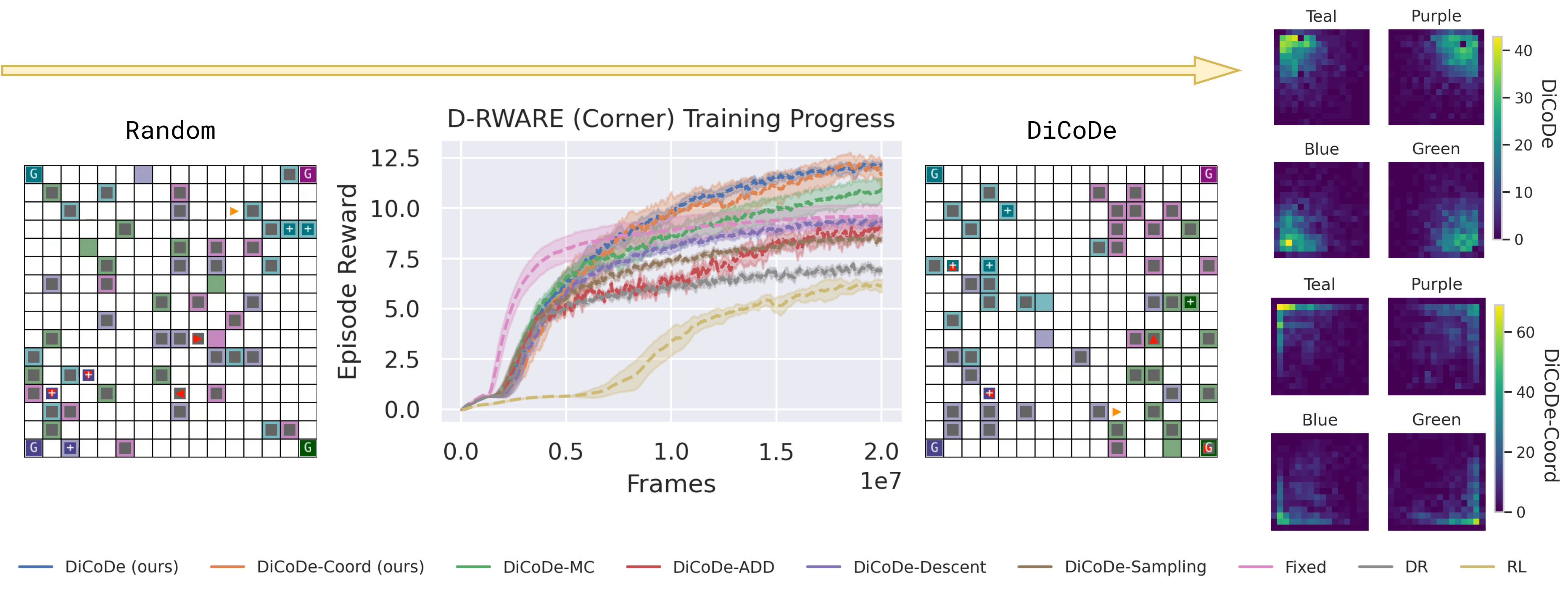
Training curves for Corner can be seen in Figure 3, left, and we provide quantitative summaries for all experiments in Table 1. These results show that DiCoDe improve multi-agent system performance considerably, converging on successful environment policy pairs with higher rewards than baselines and ablations. In particular, DiCoDe outperforms training on a fixed environment by , demonstrating the tangible benefits of considering the environment as a decision variable. Furthermore, we highlight that DiCoDe delivers more boxes on average than the RL method when measuring performance by a fixed number of policy updates with fewer samples, and more when normalized to the number of samples.
Empirically, DiCoDe continuously samples across a distribution of high-performing environments instead of collapsing to a single environment. Figure 3, right, visualises the distribution of generated post-training. DiCoDe captures the intuition that shelves should be close to goals of the same color. Furthermore, borders are left clear, possibly as navigation channels. Although DiCoDe- achieves quantitively similar rewards as the standard representation, the heat-map generated is sharper. We speculate this is related to the interpretation of gradients in the encoding of shelves. Coordinate encodings support small adaptations by moving in the direction of the critic gradient, but in the shelf mask encoding, a small step in the gradient direction leaves the manifold of valid environments. The environments generated lack rigid structure to the human eye, yet achieve impressive performance, suggesting co-design may help explore a range of environments otherwise not considered by human experts.
2) Ablation on the impact of PUG and Critic Distillation. Ablations DiCoDe-{Descent, Sampling, ADD} validate the value gain of PUG and DiCoDe-MC validates the value gain of environment critic distillation. The combined DiCoDe method outperforms DiCoDe-Descent by , DiCoDe-Sampling by , DiCoDe-ADD by and DiCoDe-MC by , showing the impact of our contributed modules. We investigate further in two directions.


First, we compare different Sampling, Descent and Universal Guidance (UG) (Bansal et al., 2023) methods compared to PUG, using the same fixed pre-trained environment critic on . In Figure 4, we observe that PUG and UG obtain similar values exceeding the other methods. This indicates carefully-designed diffusion is an effective search method over : constraint-projection leads to minimal loss in optimisation performance, noting that UG generates invalid environments. The highest-value achieved by sampling the best of uniformly sampled environments is worse in comparison to the mean of PUG, suggesting future environment design methods should rely on learnt generators rather than replay (Jiang et al., 2021b). Visualisations (see Appendix 10) verify PUG generates environments with distribution of shelves close to goals of the same colour while leaving clear navigation channels. The baseline methods are in local minima, in particular the colour of shelves which are hard to optimise as switching colours is a large jump in .
| Scenario | DiCoDe | Baselines | Ablations | ||||||
| Fixed | DR | Desc. | Sampl. | ADD | MC | ||||
| Corner | |||||||||
| WFCRL2 | — | — | |||||||
| WFCRL4 | — | — | |||||||
| WFCRL8 | — | — | |||||||
| WFCRL16 | — | — | |||||||
| ONav | — | — | |||||||
Second, we analyse the environment critic targets generated by DiCoDe against DiCoDe-MC during a training run. Using confers several noticeable properties in favour of DiCoDe. Notice in Figure 5 how has a lower maximum and higher minimum than , supporting the claim that critic-generated targets may filter out stochasticity within rollouts of fixed . Extreme values of may reflect luck rather than true environment quality. Additionally, up until approximately step , remains below due to sampling rollout returns that do not reflect the latest policy. Conversely, minimum increases earlier, showing mitigation of policy-shift. These results demonstrate critic distillation confers a stable and accurate training signal, improving sample efficiency.
3) Generalisation to continuous environments and comments on scalability. We evaluate our method on four windfarm management scenarios, WFCRL-{2,4,8,16}, with the suffix denoting the number of turbines to be placed on a square map. There is a minimum distance constraint between turbines and agents policies control the yaw of each turbine to adjust to wind conditions. Each setup is trained for frames across environments. Additionally, we examine applicability to the multi-agent navigation VMAS-ONav scenario, equipped with obstacles that can be reconfigured in their local neighbourhoods. This is trained on frames across environments.
Table 1 shows average returns after training. In these scenarios, the proposed algorithm outperforms baselines by achieving higher episode returns across averaging above Fixed environments, above RL (despite training on fewer environments) and above domain randomisation.
When fine-tuning for WFCRL, we found it essential to anneal the guidance weights in training as discussed in Section 3.4, reflecting PUG enables control over the amount of environment exploration during training. In samples of the windfarms generated by DiCoDe (Figure 2), we see the guided diffusion model learns to split turbines into two groups and distribute them in the major axis of wind to reduce turbulence. These results demonstrate the efficacy of DiCoDe across a wide range of environments, both continuous and discrete, whereas prior methods limit implementation to a single class of scenarios.

In Figure 6, we plot the progression of performance as the number of turbines increase which corresponds to increasing number of agents and environment design dimensionality. In contrast to the severe drop-off of RL performance past turbines, DiCoDe maintains performance gains, demonstrating the scalability of our approach. The computational complexity of DiCoDe does not scale with the number of training iterations, taking a constant amount of time each iteration, and requires substantially fewer samples. Our implementations are not production optimised and experiments ran on heterogenous hardware, thus we do not report exact wall-clock times, but note that DiCoDe took significantly less time than the RL approach in our setup. As environment design occurs orders of magnitude less frequently than environment sampling, we emphasise sample efficiency as a more accurate indicator of real-world time complexity.

In Figure 7, we visualise representative examples of environments generated by DiCoDe and baselines. In both the ONav and WFCRL4 environments, the DiCoDe-generated examples exhibit structures that lie closer to the boundary of feasible design space, distinguishing them clearly from those produced by the prior state-of-the-art approach. We hypothesize this improvement arises from two factors. First, the sample inefficient RL method may not have fully converged to the optimal solution in the training budget. Second, the diffusion-based generative distribution more effectively captures the multi-modal clusters of performant environments than the multi-variate Gaussian representation employed in Reinforce.
5 Discussion
We introduced diffusion co-design (DiCoDe), a novel, state-of-the-art co-design framework for learning highly rewarding policy-environments pairs. DiCoDe incorporates projected universal guidance (PUG) for guiding pre-trained diffusion models and critic distillation to improve sample efficiency (by mitigating policy shift and incorporating knowledge of individual agent interactions), and coordinates these techniques with multi-agent reinforcement learning. In empirical evaluations across five scenarios encompassing warehouse delivery, windfarm management and multi-agent navigation, DiCoDe achieves in expectation reward above state-of-the-art, and above the case without co-design. Collectively, these improvements redefine the limits of multi-agent environment co-design to previously intractable domains.
There exist several directions for future work. Although our method uses an uninformative prior , there is an opportunity to exploit a different underlying distribution by incorporating foundational models (Lehman et al., 2023; Xian et al., 2023) trained on existing datasets of expert-designed environments. Secondly, DiCoDe relies on the soft co-design distribution to explore the environment design space. This can be improved by incorporating unsupervised environment design in a multi-objective framework. Finally, although our method shows strong empirical performance and is built on principled foundations, we do not provide theoretical guarantees. Theoretically examining co-design convergence is of interest.
Impact Statement
This paper presents work which advances the field of agent-environment co-design, with many potential applications across societal domains. We do not feel any consequences must be specifically highlighted.
References
- Wind power plants layouts according to arbitrary reference points, thanet, west of duddon sands, ormonde, westermost rough, horns rev 1 & 2, anholt, and london array [data set]. zenodo. Cited by: Figure 9, Figure 9.
- Trends and new practical applications for warehouse allocation and layout design: a literature review. SN Applied Sciences 5 (12), pp. 378. Cited by: §F.1.
- Time, travel, and energy in the uniform dispersion problem. IEEE Transactions on Robotics. Cited by: §1.
- Reverse-time diffusion equation models. Stochastic Processes and their Applications 12 (3), pp. 313–326. Cited by: §1.3.
- What matters for on-policy deep actor-critic methods? a large-scale study. In International conference on learning representations, Cited by: Table 3, Table 3.
- Universal guidance for diffusion models. In Proceedings of the IEEE/CVF Conference on Computer Vision and Pattern Recognition, pp. 843–852. Cited by: Appendix B, Appendix B, §1.3, §1.3, §1, §4.
- Vmas: a vectorized multi-agent simulator for collective robot learning. In International Symposium on Distributed Autonomous Robotic Systems, pp. 42–56. Cited by: §F.1, §1, §4.
- WFCRL: a multi-agent reinforcement learning benchmark for wind farm control. Advances in Neural Information Processing Systems 37, pp. 133254–133281. Cited by: §F.1, §1, §1, §4.
- TorchRL: a data-driven decision-making library for pytorch. In The Twelfth International Conference on Learning Representations, External Links: Link Cited by: §G.1.
- Offline reinforcement learning via high-fidelity generative behavior modeling. In The Eleventh International Conference on Learning Representations, External Links: Link Cited by: Appendix E.
- Scalable co-optimization of morphology and control in embodied machines. Journal of The Royal Society Interface 15 (143), pp. 20170937. Cited by: §1, §1, §2.
- Diffusion policy: visuomotor policy learning via action diffusion. The International Journal of Robotics Research, pp. 02783649241273668. Cited by: Appendix E.
- Shared experience actor-critic for multi-agent reinforcement learning. In Advances in Neural Information Processing Systems, H. Larochelle, M. Ranzato, R. Hadsell, M. F. Balcan, and H. Lin (Eds.), Vol. 33, pp. 10707–10717. External Links: Link Cited by: §1, §1.
- Constrained synthesis with projected diffusion models. Advances in Neural Information Processing Systems 37, pp. 89307–89333. Cited by: Appendix B, Appendix D, §1.3, §1.3, §1, §3.2.
- Adversarial environment design via regret-guided diffusion models. In The Thirty-eighth Annual Conference on Neural Information Processing Systems, Cited by: Appendix C, Appendix C, Appendix E, §G.1, §1, §2, §3.1, §4.
- Emergent complexity and zero-shot transfer via unsupervised environment design. Advances in Neural Information Processing Systems 33, pp. 13049–13061. Cited by: §1.2, §1, §2.
- Diffusion models beat gans on image synthesis. Advances in neural information processing systems 34, pp. 8780–8794. Cited by: §1.3, §1.3, §1.
- Constrained environment optimization for prioritized multi-agent navigation. IEEE Open Journal of Control Systems 2 (), pp. 337–355. External Links: Document Cited by: §F.1, §1, §1, §2, §3.4, §4.
- Wind plant power optimization through yaw control using a parametric model for wake effects—a cfd simulation study. Wind Energy 19 (1), pp. 95–114. Cited by: §F.1.
- DiffAxE: diffusion-driven hardware accelerator generation and design space exploration. External Links: 2508.10303, Link Cited by: Appendix E.
- Aligning optimization trajectories with diffusion models for constrained design generation. Advances in Neural Information Processing Systems 36, pp. 51830–51861. Cited by: Appendix B, Appendix D.
- Minimum constraint displacement motion planning.. In Robotics: science and systems, Vol. 6, pp. 2. Cited by: §2.
- Distilling the knowledge in a neural network. arXiv preprint arXiv:1503.02531. Cited by: §3.3.
- Denoising diffusion probabilistic models. Advances in neural information processing systems 33, pp. 6840–6851. Cited by: Appendix A, Appendix A, §F.1, §1.3.
- A review of offshore wind farm layout optimization and electrical system design methods. Journal of Modern Power Systems and Clean Energy 7 (5), pp. 975–986. Cited by: §F.1.
- Cooperative multi-agent reinforcement learning-based co-optimization of cores, caches, and on-chip network. ACM Transactions on Architecture and Code Optimization (TACO) 14 (4), pp. 1–25. Cited by: §2.
- Planning with diffusion for flexible behavior synthesis. In International Conference on Machine Learning, pp. 9902–9915. Cited by: Appendix E.
- Information theory and statistical mechanics. Physical review 106 (4), pp. 620. Cited by: §3.1.
- A note on wind generator interaction. Risø National Laboratory. Cited by: §F.1.
- Replay-guided adversarial environment design. Advances in Neural Information Processing Systems 34, pp. 1884–1897. Cited by: §2.
- Prioritized level replay. In International Conference on Machine Learning, pp. 4940–4950. Cited by: §2, §4.
- Adam: A method for stochastic optimization. In 3rd International Conference on Learning Representations, ICLR 2015, San Diego, CA, USA, May 7-9, 2015, Conference Track Proceedings, Y. Bengio and Y. LeCun (Eds.), External Links: Link Cited by: Appendix B.
- The hungarian method for the assignment problem. Naval research logistics quarterly 2 (1-2), pp. 83–97. Cited by: 2nd item.
- Design of wind farm layout for maximum wind energy capture. Renewable energy 35 (3), pp. 685–694. Cited by: §F.1.
- Handwritten digit recognition with a back-propagation network. Advances in neural information processing systems 2. Cited by: §F.1.
- Evolution through large models. In Handbook of evolutionary machine learning, pp. 331–366. Cited by: §5.
- Asynchronous methods for deep reinforcement learning. In International conference on machine learning, pp. 1928–1937. Cited by: item 2.
- Human-level control through deep reinforcement learning. nature 518 (7540), pp. 529–533. Cited by: §3.3.
- Policy invariance under reward transformations: theory and application to reward shaping. In Icml, Vol. 99, pp. 278–287. Cited by: §F.1.
- Benchmarking multi-agent deep reinforcement learning algorithms in cooperative tasks. In Proceedings of the Neural Information Processing Systems Track on Datasets and Benchmarks (NeurIPS), External Links: Link Cited by: §F.1, §4.
- Evolving curricula with regret-based environment design. In International Conference on Machine Learning, pp. 17473–17498. Cited by: §2, footnote 1, footnote 2.
- [42] Diffusion policy policy optimization. In CoRL 2024 Workshop on Mastering Robot Manipulation in a World of Abundant Data, Cited by: Appendix E.
- U-net: convolutional networks for biomedical image segmentation. In Medical image computing and computer-assisted intervention–MICCAI 2015: 18th international conference, Munich, Germany, October 5-9, 2015, proceedings, part III 18, pp. 234–241. Cited by: §F.1.
- Simultaneous determination of warehouse layout and control policies. International Journal of Production Research 53 (11), pp. 3306–3326. Cited by: §F.1, §2.
- MAESTRO: open-ended environment design for multi-agent reinforcement learning. In The Eleventh International Conference on Learning Representations, Cited by: §1.2, §2.
- E (n) equivariant graph neural networks. In International conference on machine learning, pp. 9323–9332. Cited by: §F.1, footnote 4.
- Diffusion-based curriculum reinforcement learning. Advances in Neural Information Processing Systems 37, pp. 97587–97617. Cited by: Appendix E.
- Jointly learning to construct and control agents using deep reinforcement learning. In 2019 international conference on robotics and automation (ICRA), pp. 9798–9805. Cited by: §1, §2.
- On the convergence of a sequential quadratic programming method with an augmented lagrangian line search function. Mathematische Operationsforschung und Statistik. Series Optimization 14 (2), pp. 197–216. Cited by: §F.1.
- Proximal policy optimization algorithms. arXiv preprint arXiv:1707.06347. Cited by: §3.1.
- On the stackelberg strategy in nonzero-sum games. Journal of Optimization Theory and Applications 11 (5), pp. 533–555. Cited by: §3.3.
- Denoising diffusion implicit models. In International Conference on Learning Representations, External Links: Link Cited by: Appendix A, §1.3.
- Generative modeling by estimating gradients of the data distribution. Advances in neural information processing systems 32. Cited by: §1.3, §1.3.
- Solving inverse problems in medical imaging with score-based generative models. In International Conference on Learning Representations, External Links: Link Cited by: Appendix B.
- Score-based generative modeling through stochastic differential equations. In 9th International Conference on Learning Representations, ICLR 2021, Virtual Event, Austria, May 3-7, 2021, External Links: Link Cited by: Appendix B, Appendix B, §1.3.
- Policy gradient methods for reinforcement learning with function approximation. Advances in neural information processing systems 12. Cited by: §3.3.
- Domain randomization for transferring deep neural networks from simulation to the real world. In 2017 IEEE/RSJ international conference on intelligent robots and systems (IROS), pp. 23–30. Cited by: §4.
- Deep reinforcement learning and the deadly triad. arXiv preprint arXiv:1812.02648. Cited by: §1.
- Comparative study on optimizing the wind farm layout using different design methods and cost models. Journal of Wind Engineering and Industrial Aerodynamics 146, pp. 1–10. Cited by: §F.1.
- Diffusion policies as an expressive policy class for offline reinforcement learning. In The Eleventh International Conference on Learning Representations, External Links: Link Cited by: Appendix E.
- Bayesian learning via stochastic gradient langevin dynamics. In Proceedings of the 28th international conference on machine learning (ICML-11), pp. 681–688. Cited by: Appendix B.
- Towards generalist robots: a promising paradigm via generative simulation. External Links: 2305.10455, Link Cited by: §5.
- Censored sampling of diffusion models using 3 minutes of human feedback. Advances in Neural Information Processing Systems 36, pp. 52811–52862. Cited by: §G.1.
- The surprising effectiveness of ppo in cooperative multi-agent games. Advances in neural information processing systems 35, pp. 24611–24624. Cited by: §3, §4.
- Multi-robot coordination and layout design for automated warehousing. In Proceedings of the International Symposium on Combinatorial Search, Vol. 17, pp. 305–306. Cited by: §2.
- Diffusion models for reinforcement learning: a survey. arXiv preprint arXiv:2311.01223. Cited by: Appendix E.
This section contains additional information on diffusion model background, a comparison of our work with ADD, other use cases of diffusion models in reinforcement learning settings, additional figures of our experiments, and our experiment setup.
Appendix A Denoising Diffusion Implicit Models
In this section, we provide additional details on diffusion models, primarily from the perspective of noise addition and removal based on DDPM (Ho et al., 2020).
A forward diffusion process iteratively adds Gaussian noise to a sample (environment) for timesteps according to variance schedule to form a Markov chain.
| (13) | ||||
Given target distribution , the process above defines a series of latent variable distributions . The distribution of interest is (e.g. a distribution of valid environments), which, although unknown, we may have samples for.
Consider the inverse of the forward process: the reverse diffusion process iteratively removes noise until a clean environment remains.
| (14) | ||||
Therefore, learning reduces to matching a reverse process with forward process, using samples from the desired distribution. In our use case, this is the uniform distribution of valid environments.
Ho et al. (2020) introduce DDPM as a concrete method to learn Equation 14. First, assume a linear noise schedule . We can consider learning a simplified approximation (parameterised by ) of the evidence-based lower bound for with surrogate error function using standard gradient descent techniques. The loss is defined as
| (15) | ||||
where is unit Gaussian noise, is uniformly sampled between and is a training sample. In other words, attempts to estimate the time-conditioned noise. It is possible to sample from the target distribution by following the reverse Markov process:
| (16) | ||||
In later work, Song et al. (2021a) construct non-Markovian diffusion processes with denoising diffusion implicit models (DDIM) to speed up the reverse sampling process; their method uses the same training procedure as DDPMs. This relies on as a predictor of as in Equation 9. In our implementation of DiCoDe, we train the diffusion model as in DDPM (Equation 15).
Appendix B Universal Guidance and Projected Diffusion Models
Recall the score decomposition in Equation 5, which is conditioned on diffusion time . Bansal et al. (2023) introduce universal guidance to skip conditioning the classifier on noisy images. Instead, they leverage the information within the expected clean image. Assuming the underlying process is DDIM, forward guidance is defined as
| (17) |
where is the guidance strength hyperparameter and is a classifier network. It is possible to use in place of the original estimated noise in the reverse process. In addition to forward guidance, Bansal et al. (2023) introduce backward guidance and recurrence steps.
Backward guidance improves the conditional guidance bias by replacing the single step gradient, , with the linear interpolation of multiple gradient descent steps, enabling a more accurate direction towards the local minima. In practice, the backward guidance process begins with the result of forward guidance
| (18) |
and uses the Adam optimiser (Kingma and Ba, 2015) to compute the backward guided prediction as
| (19) | ||||
Recurrence steps enable inference-time scalingm. For steps and , iteratively compute
| (20) |
where is the sampling method of the chosen reverse diffusion process.
Alternative to gradient based guidance, projection methods enforce hard constraints on the generated samples and approximate the constrained score function. For example, post-processing projections (Giannone et al., 2023) can be used on the samples of diffusion models, and Song et al. (2021b, 2022) apply linear projections at each step of the diffusion process to ensure samples are consistent with measurements.
In recent work, Christopher et al. (2024) propose projected diffusion models (PDM) as a method to enforce constraints on score diffusion models. Their method may be directly applied to stochastic gradient Langevin dynamics (SGLD) (Welling and Teh, 2011) and the sampling method suggested by Song et al. (2021b). At a high level, PDM casts the reverse process as a constrained optimisation problem and theoretically justifies projecting samples onto the constrained domain (assuming a convex constraint set) at each step of the reverse process. However, PDM directly applied to DDPM or DDIM was shown to have poor empirical performance.
Appendix C Comparison to Chung et al. (2024)
DiCoDe is partially inspired by the success of ADD (Chung et al., 2024) in the domain of unsupervised environment design . However, despite structural similarities, there are key methodological differences.
DiCoDCe and ADD share the same pre-training paradigm. Divergence occurs in environment generation and environment critic training. Whereas ADD employs standard classifier guidance, we introduce projected universal guidance. Relative to classifier guidance, PUG is better suited for co-design with its constraint satisfying properties and avoidance of noise-conditioning critics. Our ablations against DiCoDe-ADD (Table 1) show PUG is a key component that leads to improvement in reward.
In environment critic training, ADD uses a differentiable regret estimator for the adversarial UED target, while we propose critic distillation in DiCoDe. These two approaches are incomparable due to the different objectives.
Appendix D General Applicability of Projected Constraints
A potential concern with PUG is whether the projection operator is widely applicable across different environment spaces. In practice, projection onto the feasible set (often referred to as post-processing projection) is well-established for a wide range of problems (Giannone et al., 2023; Christopher et al., 2024). In our settings, cardinality constraints of the number of shelves can be reduced to a scaling factor or top- sorting, and hard constraints can be enforced with off-the-shelf solvers (See Appendix F.1). In early explorative work, we experimented with applying constraints with a binary classifier added to the score estimation, however we found this led to unsatisfactory results.
Additionally, we report the fraction of invalid environments without projected constraints on the pixel domain for D-RWARE.
| Recurrences | |||||
| 1 | 72.66 | 72.66 | 60.94 | 23.44 | 0.00 |
| 8 | 98.44 | 98.44 | 98.44 | 96.88 | 87.50 |
Increasing results in the critic’s signal dominating the pre-trained diffusion model, leading to a low percentage of valid environments. This cannot be fully recovered by increasing the number of recurrence steps.
Appendix E Diffusion Models in Reinforcement Learning
Diffusion models in reinforcement learning have been utilised in systems beyond ours and Chung et al. (2024). (Zhu et al., 2023) and (Janner et al., 2022) experiment with diffusion models as a trajectory planner for robotic tasks; they leverage classifier guidance and find that physical constraints can be adequately posed as an in-painting problem. Wang et al. (2023), Chen et al. (2023), Chi et al. (2023) andRen et al. use diffusion models as an expressive policy class with success in multi-modal action and trajectory distributions. Sayar et al. (2024) use diffusion models as a goal-distribution generator for curriculum learning. Concurrently with our work, recently Ghosh et al. (2025) developed a diffusion-based hardware accelerator generator to replace reinforcement learning and sampling techniques.
Appendix F Experimental Details
We discuss the experimental setup, including scenarios, hyper-parameters and compute required.
F.1 Scenarios
Designable Multi-Agent Warehouse. Warehouse layout design and application is an important real-world problem, accounting for over of logistics costs (Roodbergen et al., 2015), inciting significant research interest: the recent survey by Albert et al. (2023) reviewed papers over a -year timeframe. Multi-robot warehouse (RWARE) (Papoudakis et al., 2021) is a widely used MARL benchmark inspired by real-world warehouse management tasks. In RWARE, a team of robots collaboratively pick up (uniformly sampled) requested boxes from shelves and deliver them to goals — a reward is received each time a box is delivered, and empty boxes must be returned to shelves. Shelves act as obstacles, interfering with agent navigation — a designer must strike a careful balance between placing shelves close to goals and freeing movement channels.

As part of our contributions, we fork RWARE and propose a new environment Designable Multi-Robot Warehouse (D-RWARE), shown in Figure 8. D-RWARE extends RWARE with a number of improvements including an environment design API, coloured objectives, and reward shaping. The D-RWARE scenario is a configurable grid world with a fixed number of robots, shelves and goals. Agents interact with the world using a discrete action space: movement in the four cardinal directions and picking/dropping boxes on their square. They receive observations on (shelves, boxes and teammates) within a certain distance from the agent, heuristics to the nearest (requested box, goal and empty shelf), and personal status information. We select a convolutional neural network (CNN) (LeCun et al., 1989) architecture, followed by an MLP head for the policy, and share parameters between different agents.
In RWARE, an agent receives a reward of for each box delivered to a goal. We apply a shaped reward in D-RWARE to reduce the sparseness of the reward signal: part of the reward allocation is transferred to picking up a requested box, bringing requested boxes closer to goals, and returning empty boxes to shelves. Because the reward shaping is potential-based333We ignore the discount factor in shaping for simplicity, so there may be minor changes to the optimal policy. (Ng et al., 1999), we can keep the original interpretation of episode returns as the count of boxes delivered.
The agent critic should be able to evaluate the expected return of a policy across different environments. We use the same UNET encoder with attention (Ronneberger et al., 2015; Ho et al., 2020) as ADD for the backbone of our critic network. The agent critic network takes in agent observations, concatenated with a global map of the environment, to estimate the expected return of the agent policy.
A key design choice of DiCoDe is selecting suitable , , and for the diffusion process; the representation can implicitly encode invariances and structural constraints. We assume goal and agent positions are known in advance, and examine two possible representations for deciding the layout of shelves.
-
•
Standard: The layout of shelves is represented as a binary mask for each colour, where each pixel represents a square in the grid world. Let denote and is the set of colours
This representation assigns each shelf to a single square in the grid world, and the natural CNN architecture choice is invariant to translations, which aids neural network training. Although adequately guides boxes of different channels to different squares and pushes real values to binary, it insufficiently constrains the number of shelves within a channel. Therefore, projection operation sorts the pixels in a channel by value, retains the specified number (shelves) of top-ranked values, followed by transformation to a binary mask. A UNET is suitable for the diffusion model , and we use the same UNET encoder architecture as the agent critic for the environment critic .
-
•
Coord: Alternatively, we can represent shelves as a set of coordinate-colour pairs.
will constrain the correct number of shelves but does not snap locations to . We use the Hungarian algorithm (Kuhn, 1955) to match shelves to the closest grid squares, where the cost function is the Manhattan distance between the shelf and the grid coordinate. Then, we move shelf coordinates linearly towards the matched grid square until the target grid square is the closest grid square for . At the end of the diffusion process, we snap shelf coordinates exactly — the prior projections guarantee this will lead to a valid environment.
Empirically, an MLP suffices for . To select a suitable architecture for the environment critic model, we evaluate444We also experiment with E(n) equivariant neural networks (Satorras et al., 2021), with unsatisfactory performance. a UNET decoder (as in the image representation) preceded by a graph attentional layer (veličković2018graphattentionnetworks): the graph attentional layer takes in the shelf coordinates as nodes, and connects edges (encoded with radial distance) from shelves to nearby grid points. Initial node encodings for shelves are one-hot encodings of the shelf colour. The grid points, after the graph attentional layer, can then be interpreted as pixels in an image by the CNN. By construction, this architecture is invariant to the permutation of shelves and also captures the spatial relationships between shelves and grid points. In the limiting case where shelf coordinates are perfectly aligned to the grid, the architecture is equivalent to representation.
Wind Farm Control (WFCRL). The increasing demand for clean energy is leading to rising industrial and academic interest in designing efficient wind farms (Wang et al., 2015; Hou et al., 2019). The primary objective of wind farm control lies in minimising wind power losses by the wake interaction (Jensen, 1983) caused by turbulence from upstream turbines; a secondary objective may be to reduce mechanical fatigue. Both the control policy and farm layout have a direct impact on this objective. To provide a tool to aid the development of agent-based wind farm control policies, Bizon Monroc et al. (2024) introduce Wind Farm Control with Reinforcement Learning (WFCRL), an open-source MARL environment for the wind farm control problem with adjustable layouts.

A WFCRL scenario consists of homogenous turbine agents spread out on a map with a minimum distance constraint (Kusiak and Song, 2010) between turbines. Agents receive local measurements of the wind conditions (speed and direction) as observation, concatenated with the layout. Using these observations, agents may adjust their yaw to balance between maximising local power product and deflecting wake away from downstream turbines. The team of turbines receive the same reward as the mean power subtracted by fatigue. The scenario’s transition function depends on an underlying wind condition simulator; we choose the FLORIS (Gebraad et al., 2016) simulator option and sample initial free wind conditions from the Weibull distribution.
In our implementation of DiCoDe for WFCRL, we parametrise the diffusion model with an MLP. We assume there are available communication links between the turbines: the policy is parameterised by an E(3)555Group of rotations, reflections and translations in 3D. equivariant graph neural network (GNN) (Satorras et al., 2021). To transform the set of turbines into a graph, we use a fully connected structure (WFCRL-2,4,8) or a closest neighbour approach (WFCRL-16), with attention weightings on each edge. Similarly, we parametrise the agent critic with E(3) invariant GNN — an equivariant GNN followed by an invariant aggregation layer. The environment critic takes in turbine positions as input without wind directions. Therefore, we use a translationally invariant GNN that is not invariant in rotations and reflections.
To enforce the minimum distance constraint, we formulate as a soft constraint to penalise constraint violations while trying to minimise movement of turbine locations; this is solved with gradient descent. To enforce hard constraint satisfaction, we apply a Sequential Least SQuares Programming (SLSQP) solver (Schittkowski, 1983) to the final layout.
Multi-agent navigation is a mandatory subroutine in robotic application settings such as warehouses, factories, or hospitality. Additionally, it is the setting considered in prior work for comparison (Gao and Prorok, 2023). We implement a multi-agent navigation scenario as a using the VMAS (Bettini et al., 2022) multi-agent physics simulator. In our formulation, each agent is spawned in a fixed position, and is rewarded for approaching a fixed goal. We parametrise the diffusion model, agent policy, agent critic and environment critic with MLPs, and set up the obstacles with a local boundary such that constraints are not necessary in the environment. We remark that because both agent critic and environment critic use the same information processing architecture, and that the environment setup is differentiable, this is an edge case of distillation where agent critic and environment critic may share parameter weights. Finally, we note that the training time on multi-agent navigation with our hyperparameter selection is an order of magnitude lower than D-RWARE (20 minutes compared to 30 hours, and that prior co-design works were often limited to only multi-agent navigation problems.
Appendix G Reproducibility Statement
We understand the importance of reproducibility, and make efforts to ensure our work is reproducible. We provide detailed explanations of our methodology in Section 3, and discuss the evaluation setup in Section 4 and Appendix F. We publicly release our training and evaluation code at https://github.com/MarkHaoxiang/diffusion-co-design, which can readily be used to reproduce all results in this paper. We used up-to-date package management practices to enable easy installation of the environment.
G.1 Hyper-parameters
We use the MAPPO implementation of TorchRL (Bou et al., 2024) and our diffusion pipeline is forked from Chung et al. (2024), which itself is a fork of Yoon et al. (2023).
| MAPPO HP | Value | ||
| D-RWARE | WFCRL | VMAS | |
| Optimiser | Adam | ||
| Learning rate annealing | Cosine (Restartless) | ||
| Initial actor LR | 3e-4 | ||
| Final actor LR | 0 | ||
| Initial critic LR | 3e-4 | ||
| Discount factor () | 0.99 | ||
| Clip ratio () | 0.2 | ||
| Max gradient norm | 1.0 | ||
| Critic loss criterion | Huber | ||
| Final critic LR | 1e-4 | 2e-4 | 1e-4 |
| GAE parameter () | 0.9 | 0.95 | 0.9 |
| Entropy coefficient | 1e-3 | 0 | 1e-3 |
| Update epochs | 5 | 8 | 10 |
| Minibatch size | 500 | 150 | 400 |
| Minibatches per epoch | 10 | 20 | 10 |
| Normalise advantage | False | True | False |
| Critic normalisation | False | True | False |
Table 3 lists the MAPPO hyper-parameters used in experiments. Table 4 lists additional hyperparameters.
| DiCoDe HP | Value | |||
| D-RWARE | D-RWARE | WFCRL | VMAS | |
| Diffusion Steps | 1000 | |||
| Diffusion Process | DDIM (50 steps) | |||
| Optimiser | Adam | – | ||
| buffer size | 8096 | – | ||
| Warmup Environment | 2048 | 400 | 400 | |
| LR | 3e-5 | 1e-4 | – | |
| 10 | 1 | 1 | ||
| Loss Criterion | MSE | Huber | – | |
| Batch size | 64 | 32 | – | |
| 3 | 3 | – | ||
| Recurrences | 8 | 4 | 8 | |
| 200 | 5 | 50 | ||
| Backward | 0 | 16 (LR=0.01) | 0 | 6 (LR=0.01) |
For other hyper-parameters not listed, please refer to the codebase with yaml configuration files.
G.2 Training Hardware
Experiments were run on several different devices.
The first device had a single NVIDIA RTX 3090 GPU with 24GB of VRAM. The device used an Intel i5-13600KF CPU with 14 cores and 64GB of RAM, running Endeavour OS.
The second device had a single NVIDA RTX 4090 GPU with 24GB of VRAM. The device used an AMD Ryzen 7 7800X3D CPU with 8 cores and 64GB of RAM, running Windows 11 Pro and WSL.
The third device had a single NVIDIA RTX 5090 GPU with 32GB of VRAM. The device used an AMD Ryzen 9 9950 CPU with 16 cores and 64GB of RAM, running Endeavour OS.
The first server has 4 NVIDIA RTX2080TI GPUs, each with 12GB of VRAM. The device used an Intel Xeon Gold 6248R CPU with 48 cores, running Ubuntu 22.04. Experiments were run with Docker.
The second server has 4 NVIDIA L40S GPUs, each with 48GB of VRAM. The device used an Intel Xeon Platinum 8452Y CPU with 72 cores, running Ubuntu 22.04. Experiments were run with Docker.
This work was performed using resources provided by the Cambridge Service for Data Driven Discovery (CSD3) operated by the University of Cambridge Research Computing Service (www.csd3.cam.ac.uk), provided by Dell EMC and Intel using Tier-2 funding from the Engineering and Physical Sciences Research Council (capital grant EP/T022159/1), and DiRAC funding from the Science and Technology Facilities Council (www.dirac.ac.uk).
Appendix H Additional Results
We visualise the environments generated by our ablations in Figure 10 for qualitative analysis. The results reveal clear, intuitive structures present in the PUG example, where navigation channels — a space of at least one cell — are present, and colours cluster together. In contrast, the examples obtained through Descent or Sampling are in local minima, particularly the colours of shelves. Additionally, the Sampling method exhibits an untraversable goal in the bottom left corner.


We provide additional examples of generated environments in the D-RWARE Corners environment, at the start and end of training, in Figures 11 and 12.


Finally, we present training curves and additional ablations in Figures 13, 14 and 15. Our results corroborate with Section 4, demonstrating that PUG diffusion models can effectively search over a constrained, continuous domain, and that DiCoDe is able to learn effective environment policy pairs in this domain.
Appendix I LLM Disclosure
We use LLM generated output for word/phrasing suggestions in writing, and error-checking. We also use Github Copilot and Claude Code for line-level code auto-completion, and to assist in figure generation (with data processing written by hand).
Appendix J Software Dependencies
We use uv for our package management. Table 5 shows the core dependencies used in this project.
| Package Name | License |
| matplotlib | PSF |
| numpy | BSD |
| rware | MIT |
| ADD | CC BY-NC 4.0 |
| torchrl | MIT |
| torch | BSD |
| wandb | MIT |
| hydra-core | MIT |
| pydantic | MIT |
| torch-geometric | MIT |
| torch-scatter | MIT |
| wfcrl | Apache 2.0 |
| seaborn | BSD |
| scipy | BSD |
| uv | Apache 2.0 |
| vmas | GPL-3.0 |