跳到论文正文
W Papers独立论文阅读器 arXiv:2511.02517 论文正文 计算阅读时间 · 0%
引用这篇论文根据当前论文元数据生成,正式投稿前建议核对。


License: CC BY 4.0
arXiv:2511.02517v3 [math.SP] 09 Jun 2026

Nearly optimal spectral gaps for random Belyi surfaces

Yang Shen Fudan University, Shanghai, China shenwang@fudan.edu.cn and Yunhui Wu Tsinghua University, Beijing, China yunhui_wu@tsinghua.edu.cn
Abstract.

In this paper, we show that a random hyperbolic surface in the Brooks-Makover model has a spectral gap greater than (14−clog⁡n)\left(\frac{1}{4}-\frac{c}{\log n}\right) for some universal constant c>0c>0 , confirming the nearly optimal spectral gap conjecture in this model.

2020 Mathematics Subject Classification:
58J50, 05C80, 57K20

1. Introduction

Let XgX_{g} be a closed hyperbolic surface of genus gg, and let λ1​(Xg)\lambda_{1}(X_{g}) be its first Laplacian eigenvalue. It is known from e.g. Huber [24] or Cheng [15] that

lim supg→∞λ1​(Xg)≤14\limsup\limits_{g\to\infty}\lambda_{1}(X_{g})\leq\frac{1}{4}

for any sequence of closed hyperbolic surfaces {Xg}g≥2\{X_{g}\}_{g\geq 2}. A long-standing conjecture of Buser [49] predicted the sharpness of this bound, i.e., the existence of a sequence {Xg}\{X_{g}\} of closed hyperbolic surfaces with λ1​(Xg)→14\lambda_{1}(X_{g})\to\frac{1}{4} as g→∞g\to\infty. This was first achieved by Hide-Magee [27], who essentially proved the nearly optimal spectral gap for random covers of a cusped hyperbolic surface. For closed surfaces, research has focused on three prominent randomness models: the Brooks-Makover model, the Weil-Petersson model, and the covering model. It is widely conjectured that a random closed hyperbolic surface in all these three models has nearly optimal spectral gap. In what follows, we briefly review the progress toward this conjecture across the three models.

Brooks-Makover Model: Brooks and Makover [11] proved that a random closed hyperbolic surface in their model has a uniform spectral gap c>0c>0, where the constant cc is implicit. This was not only the first proof of a uniform spectral gap for random closed hyperbolic surfaces but also remains the only such result within their specific model.

Weil-Petersson Model: The study of spectral gaps for random closed hyperbolic surfaces in this model began with Mirzakhani [47], who proved a lower bound 0.002470.00247. This bound was significantly improved to (316−ϵ)\left(\frac{3}{16}-\epsilon\right) for any ϵ>0\epsilon>0 by Wu-Xue [63] using a completely different method, a result independently obtained by Lipnowski-Wright [36]. In a series of subsequent works, Anantharaman-Monk raised the lower bound further to (29−ϵ)\left(\frac{2}{9}-\epsilon\right) in [2] and eventually to (14−ϵ)\left(\frac{1}{4}-\epsilon\right) in the remarkable work [3], resolving the nearly optimal spectral gap conjecture for the Weil-Petersson model. Most recently, Hide-Macera-Thomas [26] provided an alternative proof via the polynomial method, additionally refining the ϵ\epsilon term to a significant explicit polynomial error of order 1gδ\frac{1}{g^{\delta}} for some uniform δ>0\delta>0.

Covering Model: Magee-Naud-Puder [42] proved that for any ϵ>0\epsilon>0 and any fixed closed hyperbolic surface XX, the eigenvalues (with multiplicity) of a random covering surface of XX within (0,316−ϵ)\left(0,\frac{3}{16}-\epsilon\right) coincide with those of XX. In a recent remarkable work [44], Magee-Puder-van Handel used the polynomial method to improve the bound from (316−ϵ)\left(\frac{3}{16}-\epsilon\right) to (14−ϵ)\left(\frac{1}{4}-\epsilon\right), resolving the nearly optimal spectral gap conjecture for the covering model. Hide-Macera-Thomas [25] refined the term ϵ\epsilon to a polynomial error of order 1gb\frac{1}{g^{b}} for some uniform b>0b>0.

Recall that for all n≥1n\geq 1, set

ℱn⋆={(Γ,𝒪);Γ​ is a 3−regular graph with 2​n vertices,𝒪​ is an orientation on ​Γ}.\mathcal{F}_{n}^{\star}=\left\{(\Gamma,\mathcal{O});\ \begin{matrix}\Gamma\text{ is a $3-$regular graph with $2n$ vertices,}\\ \mathcal{O}\text{ is an orientation on }\Gamma\end{matrix}\right\}.

As introduced by Brooks-Makover [11], there are two associated hyperbolic surfaces for each (Γ,𝒪)∈ℱn⋆(\Gamma,\mathcal{O})\in\mathcal{F}_{n}^{\star}: a cusped hyperbolic surface SO​(Γ,𝒪)S^{O}(\Gamma,\mathcal{O}) which is obtained by gluing 2​n2n hyperbolic ideal triangles in a certain way, and a closed hyperbolic surface SC​(Γ,𝒪)S^{C}(\Gamma,\mathcal{O}) which is the conformal compactification of SO​(Γ,𝒪)S^{O}(\Gamma,\mathcal{O}) by filling in all the cusps. It is known that such constructions produce all the so-called Belyi surfaces that are dense in the space of all Riemann surfaces in a certain sense (see e.g. [4, 20]). For each nn, the set ℱn⋆\mathcal{F}_{n}^{\star} is finite, and hence there is a classical probability measure denoted by ProbBMn\textnormal{Prob}_{\textnormal{BM}}^{n} on ℱn⋆\mathcal{F}_{n}^{\star}, which was introduced by Bollabás [6].

As mentioned previously, the Brooks-Makover model has stood as the final piece of the puzzle among the three models of random closed hyperbolic surfaces, being the only one for which the nearly optimal spectral gap conjecture was still unproven. Our work completes this picture by resolving the conjecture (as e.g. formulated in [52, Page 71]). Specifically, we prove

Theorem 1.1.

There exists a universal constant c>0c>0 such that the following limit holds:

limn→∞ProbBMn​((Γ,𝒪)∈ℱn⋆;λ1​(SC​(Γ,𝒪))>14−clog⁡n)=1.\lim\limits_{n\to\infty}\textnormal{Prob}_{\textnormal{BM}}^{n}\left((\Gamma,\mathcal{O})\in\mathcal{F}_{n}^{\star};\ \lambda_{1}\left(S^{C}(\Gamma,\mathcal{O})\right)>\frac{1}{4}-\frac{c}{\log n}\right)=1.

We will first show that the spectral gap of a cusped hyperbolic surface becomes larger after compactification (see Proposition 2.1). Therefore, to prove Theorem 1.1, it suffices to show that a random cusped hyperbolic surface SO​(Γ,𝒪)S^{O}(\Gamma,\mathcal{O}) has no eigenvalue in (0,14−clog⁡n)\left(0,\frac{1}{4}-\frac{c}{\log n}\right). Our approach is inspired by the work [44] of Magee-Puder-van Handel that builds upon the polynomial method in e.g. [13, 14, 41]. Meanwhile, we believe that the novel ingredients developed in this work will find further applications in studying the asymptotics of other geometric quantities in this model of random hyperbolic surfaces.

For more related results of spectral gaps on random hyperbolic surfaces, one may refer to e.g. [29, 28, 59] for the Weil-Petersson model and to e.g. [43, 27, 38] for the covering model. Similar results on spectral gaps also hold for random graphs. Alon [1] conjectured and Friedman [19] proved that a random d−d-regular (d≥3)(d\geq 3) graph has nearly optimal spectral gap, as the number NN of vertices goes to infinity. A recent breakthrough of Huang-Mckenzie-Yau [30] proved that as N→∞N\to\infty, about 69%69\% d−d-regular graphs with NN vertices are Ramanujan graphs, that is, have optimal spectral gaps. It is natural to ask whether an analogous result holds for all these three models of random closed hyperbolic surfaces. That is,

Question 1.

Does there exist a constant c∈(0,1)c\in(0,1) such that

limg→∞Prob​(λ1​(X)≥14)=c​?\lim\limits_{g\to\infty}\textnormal{Prob}\left(\lambda_{1}(X)\geq\frac{1}{4}\right)=c?

where the constant c>0c>0 may be different for these three models of random closed hyperbolic surfaces.

The existence of infinite families of Ramanujan graphs was first proved in [39, 46, 45]. We remark here that it remains even open that there exists a closed hyperbolic surface XgX_{g} of genus gg such that λ1​(Xg)≥14\lambda_{1}(X_{g})\geq\frac{1}{4} for all g≥2g\geq 2. It is known from [61, 16, 18] that such so-called Ramanujan surfaces exist in genera 22 to 77, 1414 and 1717. In this paper, based on [7] we show that Ramanujan surfaces also exist in genera

g​(N)=1+N2​(N−6)24​∏p∣N(1−1p2)g(N)=1+\frac{N^{2}(N-6)}{24}\prod_{p\mid N}\Big(1-\frac{1}{p^{2}}\Big)

whenever 7≤N≤2267\leq N\leq 226. See Theorem 2.5.

Strategy on the proof of Theorem 1.1. We first give a new geometric description for each cusped hyperbolic surface SO​(Γ,𝒪)S^{O}(\Gamma,\mathcal{O}) in the Brooks-Makover model.

For n≥1n\geq 1, assume that S6​nS_{6n} is the permutation group of 6​n6n elements. Set

ℰn={(σ,τ);σ,τ∈S6​n, σ has order 2 and no fixed point,τ has order 3 and no fixed point.}.\mathcal{E}_{n}=\left\{(\sigma,\tau);\ \begin{matrix}\sigma,\tau\in S_{6n},\text{ $\sigma$ has order $2$ and no fixed point,}\\ \text{$\tau$ has order $3$ and no fixed point}.\end{matrix}\right\}.

For each (σ,τ)∈ℰn(\sigma,\tau)\in\mathcal{E}_{n}, it induces a group homomorphism

Φ​(σ,τ):PSL​(2,ℤ)→S6​n,\Phi(\sigma,\tau):\textnormal{PSL}(2,\mathbb{Z})\to S_{6n},

which corresponds to a degree 6​n6n covering hyperbolic surface SO​(σ,τ)S^{O}(\sigma,\tau) of the modular surface ℍ/PSL​(2,ℤ)\mathbb{H}/\textnormal{PSL}(2,\mathbb{Z}). For each cusped hyperbolic surface SO​(Γ,𝒪)S^{O}(\Gamma,\mathcal{O}) in the Brooks-Makover model, it is isometric to certain SO​(σ,τ)S^{O}(\sigma,\tau) (see e.g. Theorem 2.8). One major difference between the Brooks-Makover model and the covering model of cusped hyperbolic surfaces (see e.g. [27]) is as following: All degree nn covering hyperbolic surfaces of a fixed cusped hyperbolic surface XX correspond to all group homomorphisms ϕ∈Hom​(π1​(X),Sn)\phi\in\textnormal{Hom}(\pi_{1}(X),S_{n}), while the set of all hyperbolic surfaces SO​(σ,τ)S^{O}(\sigma,\tau) in the Brooks-Makover model corresponds to an “asymptotic measure zero” subset of

Hom​(PSL​(2,ℤ),S6​n)\textnormal{Hom}(\textnormal{PSL}(2,\mathbb{Z}),S_{6n})

as n→∞n\to\infty.

Next, we adapt the polynomial method for the strong convergence of random matrices, introduced by Chen, Garza-Vargas, Tropp and van Handel in [13], and its generalization to the strong convergence of surface groups by Magee, Puder and van Handel [44], to study the strong convergence property of PSL​(2,ℤ)\textnormal{PSL}(2,\mathbb{Z}) in the Brooks-Makover model. We prove two important propositions: Proposition 4.1 and 4.3 that correspond to Assumption 1.3 and 1.4 in [44], respectively. Recall that the group PSL​(2,ℤ)\textnormal{PSL}(2,\mathbb{Z}) has a unitary representation called the regular representation:

λ:PSL​(2,ℤ)→𝒰​(ℓ2​(PSL​(2,ℤ))),λ​(γ)​[f]​(x)=f​(γ−1​x)\lambda:\textnormal{PSL}(2,\mathbb{Z})\to\mathcal{U}(\ell^{2}(\textnormal{PSL}(2,\mathbb{Z}))),\ \lambda(\gamma)[f](x)=f(\gamma^{-1}x)

for any f∈ℓ2​(PSL​(2,ℤ))f\in\ell^{2}\left(\textnormal{PSL}(2,\mathbb{Z})\right) and x∈PSL​(2,ℤ)x\in\textnormal{PSL}(2,\mathbb{Z}). The regular representation could also be linearly extended to ℂ​[PSL​(2,ℤ)]\mathbb{C}\left[\textnormal{PSL}(2,\mathbb{Z})\right] where

ℂ[PSL(2,ℤ)]={∑γ∈PSL​(2,ℤ)aγγ;aγ∈ℂ,aγ≠0 for finitely many γ′s}.\mathbb{C}\left[\textnormal{PSL}(2,\mathbb{Z})\right]=\left\{\sum\limits_{\gamma\in\textnormal{PSL}(2,\mathbb{Z})}a_{\gamma}\gamma;\ a_{\gamma}\in\mathbb{C},\ a_{\gamma}\neq 0\text{ for finitely many }\gamma^{\prime}s\right\}.

For any n≥1n\geq 1, denote by 𝒰​(n)\mathcal{U}(n) the group of n×nn\times n complex unitary matrices. The 6​n−6n-dimensional linear representation of S6​nS_{6n} by permutation matrices has a (6​n−1)−(6n-1)-dimensional irreducible subrepresentation

std:S6​n→𝒰​(6​n−1)\textnormal{std}:S_{6n}\to\mathcal{U}(6n-1)

obtained by removing non-zero invariant vectors. Define

tr ​Πγ:ℰn→ℝ\textnormal{tr }\Pi_{\gamma}:\mathcal{E}_{n}\to\mathbb{R}

as

tr ​Πγ​(σ,τ)​=def​16​n​Tr ​(std∘Φ​(σ,τ)​(γ)),\textnormal{tr }\Pi_{\gamma}(\sigma,\tau)\overset{\mathrm{def}}{=}\frac{1}{6n}\textnormal{Tr }\left(\textnormal{std}\circ\Phi(\sigma,\tau)(\gamma)\right),

where Tr ​(⋅)\textnormal{Tr }(\cdot) is the trace of a unitary matrix in 𝒰​(6​n−1)\mathcal{U}(6n-1). Denote by 𝔼n​[⋅]\mathbb{E}_{n}\left[\cdot\right] the expectation on ℰn\mathcal{E}_{n}. The first proposition is as follows.

Proposition 1.2 (=Proposition 4.1).

There exists a sequence {ui​(γ)}i≥0⊂ℝ\{u_{i}(\gamma)\}_{i\geq 0}\subset\mathbb{R} for all γ∈PSL​(2,ℤ)\gamma\in\textnormal{PSL}(2,\mathbb{Z}) such that u0​(γ)=ρ​(λ​(γ))u_{0}(\gamma)=\rho(\lambda(\gamma)) and

|𝔼n​[tr ​Πγ]−∑i=0m−1ui​(γ)(6​n)i|≤(18​m)18​m(6​n)m\left|\mathbb{E}_{n}\left[\textnormal{tr }\Pi_{\gamma}\right]-\sum\limits_{i=0}^{m-1}\frac{u_{i}(\gamma)}{(6n)^{i}}\right|\leq\frac{(18m)^{18m}}{(6n)^{m}}

for all m≥|γ|+1m\geq|\gamma|+1 and n≥18​m18n\geq 18m^{18}.

Assume (σ,τ)∈ℰn(\sigma,\tau)\in\mathcal{E}_{n}, then there are two related group homomorphisms

Φ​(σ,τ):PSL​(2,ℤ)→S6​n​ and ​Φ~​(σ,τ):F2→S6​n.\Phi(\sigma,\tau):\textnormal{PSL}(2,\mathbb{Z})\to S_{6n}\text{ and }\tilde{\Phi}(\sigma,\tau):\textbf{F}_{2}\to S_{6n}.

To prove Proposition 1.2, it suffices to count the number of fixed points of permutation Φ~​(σ,τ)​(ω)​(ω∈F2)\tilde{\Phi}(\sigma,\tau)(\omega)\ (\omega\in\textbf{F}_{2}). Inspired by the work of Puder-Parzanchevski [53], we construct two graphs Γ​(σ,τ)\Gamma(\sigma,\tau) and ΓX​(ω)¯\overline{\Gamma_{X}(\omega)}, then the set of fixed points of Φ~​(σ,τ)​(ω)\tilde{\Phi}(\sigma,\tau)(\omega) corresponds to the set of certain graph homomorphisms f¯:ΓX​(ω)¯→Γ​(σ,τ)\overline{f}:\overline{\Gamma_{X}(\omega)}\to\Gamma(\sigma,\tau). Such graph homomorphisms could be decomposed into two parts: surjective homomorphisms g:ΓX​(ω)¯→Γg:\overline{\Gamma_{X}(\omega)}\to\Gamma and injective homomorphisms ι:Γ→Γ​(σ,τ)\iota:\Gamma\to\Gamma(\sigma,\tau). In Section 3.2.1, we deal with the part of injective homomorphisms, and calculate the expected value of the number of such homomorphisms (see Proposition 3.2 and 3.4). In Section 3.2.2, we introduce an algorithm to analyze the properties of such surjective homomorphisms. Together with these two parts, we calculate the expected value 𝔼n​[fixω]\mathbb{E}_{n}[\textnormal{fix}_{\omega}] for any fixed ω∈F2\omega\in\textbf{F}_{2} (see Proposition 3.7). Using all these properties, we will complete the proof of Proposition 1.2.

Recall that α∈ℂ​[PSL​(2,ℤ)]\alpha\in\mathbb{C}[\textnormal{PSL}(2,\mathbb{Z})] is called self-adjoint if

α=∑γ∈PSL​(2,ℤ)aγ​γ=∑γ∈PSL​(2,ℤ)aγ¯​γ−1.\alpha=\sum\limits_{\gamma\in\textnormal{PSL}(2,\mathbb{Z})}a_{\gamma}\gamma=\sum\limits_{\gamma\in\textnormal{PSL}(2,\mathbb{Z})}\overline{a_{\gamma}}\gamma^{-1}.

From Proposition 1.2, the coefficient u1​(⋅)u_{1}(\cdot) gives a functional on ℂ​[PSL​(2,ℤ)]\mathbb{C}[\textnormal{PSL}(2,\mathbb{Z})]. The second proposition is as follows.

Proposition 1.3 (=Proposition 4.3).

For every self-adjoint α∈ℂ​[PSL​(2,ℤ)]\alpha\in\mathbb{C}[\textnormal{PSL}(2,\mathbb{Z})], we have

lim supp→∞|u1​(αp)|1p≤‖λ​(α)‖,\limsup\limits_{p\to\infty}\left|u_{1}(\alpha^{p})\right|^{\frac{1}{p}}\leq||\lambda(\alpha)||,

where the right hand side is the operator norm.

It is known from e.g. [5, Theorem 3.38] that λ1​(ℍ/PSL​(2,ℤ))>14\lambda_{1}(\mathbb{H}/\textnormal{PSL}(2,\mathbb{Z}))>\frac{1}{4}. Finally, based on Proposition 1.2 and 1.3, we finish the proof of Theorem 1.1 following the arguments in [25, 48, 44].

Plan of the paper. In Section 2, we revisit the construction of the Brooks–Makover model and furnish it with a novel geometric characterization; we further establish a useful inequality relating the spectral gap of a cusped hyperbolic surface to that of its conformal compactification. In Section 3, we study certain group homomorphisms and calculate the expected value 𝔼n​[fixω]\mathbb{E}_{n}[\textnormal{fix}_{\omega}] for any fixed ω∈F2\omega\in\textbf{F}_{2}, which is essential in the proof of Proposition 1.2. In Section 4, we prove the strong convergence property of PSL​(2,ℤ)\textnormal{PSL}(2,\mathbb{Z}) and complete the proof of Theorem 1.1. In the Appendix, we prove an analogue of Theorem 1.1 for the cusped case, building on Propositions 1.2 and 1.3.

Acknowledgment. We are very grateful to Bram Petri for invaluable discussions on the new description of the Brooks-Makover model and his comment on this paper. We also thank Yuxin He, Yuhao Xue and Haohao Zhang for many helpful discussions and suggestions on this project. We are also grateful to Doron Puder, Joe Thomas and Ramon van Handel for their interests and comments on this paper. The first named author is supported by the NSFC grant No. 12401081, and the second named author is partially supported by the NSFC grant No. 12425107 and 12361141813.

2. Brooks-Makover Model

In this section, we recall the construction of random hyperbolic surfaces by Brooks-Makover in [11], and introduce an alternative description. Moreover, we also provide a useful inequality relating the spectral gap of a cusped hyperbolic surface to that of its conformal compactification.

2.1. Brooks-Makover random hyperbolic surfaces

Brooks and Makover [11] established a model of random hyperbolic surfaces. For each n≥1n\geq 1, denote by

ℱn​=def​{all partitions of ​{1,2,…,6​n}​ into pairs}.\mathcal{F}_{n}\overset{\mathrm{def}}{=}\{\text{all partitions of }\{1,2,...,6n\}\text{ into pairs}\}.

Then the cardinality satisfies

|ℱn|=1(3​n)!×(6​n2)×(6​n−22)×⋯×(22)=(6​n)!23​n​(3​n)!.|\mathcal{F}_{n}|=\frac{1}{(3n)!}\times\binom{6n}{2}\times\binom{6n-2}{2}\times\cdots\times\binom{2}{2}=\frac{(6n)!}{2^{3n}(3n)!}.

Assume that there are 2​n2n vertices {v1,…,v2​n}\{v_{1},...,v_{2n}\}, and for each vertex vi​(1≤i≤2​n)v_{i}\ (1\leq i\leq 2n), there are 33 half-edges {3​i−2, 3​i−1, 3​i}\{3i-2,\ 3i-1,\ 3i\} emanating from it. For any element

𝒫=⟨j1​k1⟩​…​⟨j3​n​k3​n⟩∈ℱn,\mathcal{P}=\langle j_{1}k_{1}\rangle...\langle j_{3n}k_{3n}\rangle\in\mathcal{F}_{n},

gluing the half-edges jtj_{t} and ktk_{t} (1≤t≤3​n)(1\leq t\leq 3n) together, one may obtain a 3−3-regular graph Γ​(𝒫)\Gamma(\mathcal{P}) with 2​n2n vertices. Hence ℱn\mathcal{F}_{n} is a set of certain 3−3-regular graphs.

Let Γ\Gamma be a 3−3-regular graph and V​(Γ)V(\Gamma) be the set of vertices. An orientation 𝒪\mathcal{O} on Γ\Gamma is an assignment, for each vertex v∈V​(Γ)v\in V(\Gamma), of a cyclic order for the three edges emanating from vv. Denote by

ℱn⋆​=def​{(Γ,𝒪);Γ​ is a 3−regular graph with 2​n vertices,𝒪​ is an orientation on ​Γ}.\mathcal{F}_{n}^{\star}\overset{\mathrm{def}}{=}\left\{(\Gamma,\mathcal{O});\ \begin{matrix}\Gamma\text{ is a $3-$regular graph with $2n$ vertices},\\ \mathcal{O}\text{ is an orientation on }\Gamma\end{matrix}\right\}.

Then we have

(1) |ℱn⋆|=|ℱn|×22​n=(6​n)!2n​(3​n)!.\displaystyle|\mathcal{F}_{n}^{\star}|=|\mathcal{F}_{n}|\times 2^{2n}=\frac{(6n)!}{2^{n}(3n)!}.

Now we recall the construction of Brooks and Makover in [11]. Up to a Möbius transformation, one may assume that a hyperbolic ideal triangle TT always has vertices 0,10,1 and ∞\infty. The ideal triangle TT has a natural clockwise orientation

(i, 1+i,1+i2).\left(\textbf{i},\ 1+\textbf{i},\ \frac{1+\textbf{i}}{2}\right).

As in Figure 1, the clockwise orientation induces a direction on each side of TT. The points {i, 1+i,1+i2}\left\{\textbf{i},\ 1+\textbf{i},\ \frac{1+\textbf{i}}{2}\right\} are called the mid-points of three sides of TT.

Refer to caption
Figure 1. The standard hyperbolic ideal triangle TT

Given an element (Γ,𝒪)∈ℱn⋆(\Gamma,\mathcal{O})\in\mathcal{F}_{n}^{\star}, we replace each vertex v∈V​(Γ)v\in V(\Gamma) by a copy of TT, three half-edges emanating from vv correspond to three sides of TT such that the natural clockwise orientation of TT coincides with the orientation of Γ\Gamma at the vertex vv. If two vertices of Γ\Gamma are joined by an edge, we glue the two copies of TT along the corresponding sides subject to the following conditions:

  1. (1)

    the mid-points of two sides are glued together;

  2. (2)

    the gluing preserves the orientations of two copies of TT.

As in [11], the surface SO​(Γ,𝒪)S^{O}(\Gamma,\mathcal{O}) is uniquely determined by the two conditions above and is a cusped hyperbolic surface with area equal to 2​π​n2\pi n. We remark here that orientation-preserving means that two sides are glued together via reverse directions. As in Figure 2, the ideal triangle TT has three sides a,b,ca,\ b,\ c with orientation (a​b​c)(abc), and the ideal triangle T′T^{\prime} has three sides a′,b′,c′a^{\prime},\ b^{\prime},\ c^{\prime} with orientation (a′​b′​c′)(a^{\prime}b^{\prime}c^{\prime}). If we glue the sides aa and a′a^{\prime} together such that the orientations of TT and T′T^{\prime} are preserved, then we obtain a quadrilateral.

Refer to caption
Figure 2. Orientation-preserving
Definition.

The compact Riemann surface SC​(Γ,𝒪)S^{C}(\Gamma,\mathcal{O}) is defined as the conformal compactification of SO​(Γ,𝒪)S^{O}(\Gamma,\mathcal{O}) by filling in all the punctures.

For any fixed n∈ℕn\in\mathbb{N}, ℱn⋆\mathcal{F}_{n}^{\star} is finite, hence there is a classic probability measure ProbBMn\textnormal{Prob}_{\textnormal{BM}}^{n} on it. For any random variable f:ℱn⋆→ℝf:\mathcal{F}_{n}^{\star}\to\mathbb{R}, let 𝔼BMn​[f]\mathbb{E}_{\textnormal{BM}}^{n}[f] be its expected value. More precisely,

ProbBMn​(𝒜)=|𝒜||ℱn⋆|​ and ​𝔼BMn​[f]=∑(Γ,𝒪)∈ℱn⋆f​(Γ,𝒪)|ℱn⋆|,\textnormal{Prob}_{\textnormal{BM}}^{n}(\mathcal{A})=\frac{|\mathcal{A}|}{|\mathcal{F}_{n}^{\star}|}\text{ \ and \ }\mathbb{E}_{\textnormal{BM}}^{n}[f]=\frac{\sum\limits_{(\Gamma,\mathcal{O})\in\mathcal{F}_{n}^{\star}}f(\Gamma,\mathcal{O})}{|\mathcal{F}_{n}^{\star}|},

where 𝒜⊂ℱn⋆\mathcal{A}\subset\mathcal{F}_{n}^{\star} is a subset. It is known from [11, Theorem 2.1 & Theorem 4.3] that there exists a uniform constant c>0c>0 such that

(2) limn→∞ProbBMn​(genus​(SO​(Γ,𝒪))≥c⋅n)=1.\lim\limits_{n\to\infty}\textnormal{Prob}_{\textnormal{BM}}^{n}\left(\mathrm{genus(S^{O}(\Gamma,\mathcal{O}))}\geq c\cdot n\right)=1.

One may also refer to e.g. [20, 51, 12, 58, 37, 21] for related results on this random surface model.

2.2. Comparison of eigenvalues

In this subsection, we show that the spectral gap becomes larger after conformal compactification. More precisely,

Proposition 2.1.

Let SOS^{O} be a non-compact hyperbolic surface of finite area with genus ≥2\geq 2, and let SCS^{C} be the conformal compactification of SOS^{O} obtained by filling in all the cusps of SOS^{O}, then

λ1​(SC)>RayQ​(SO)​=def​inff∈L2​(SO),∫SOf=0∫SO|∇f|2​dvolO∫SOf2​dvolO,\lambda_{1}(S^{C})>\textnormal{RayQ}(S^{O})\overset{\mathrm{def}}{=}\inf\limits_{f\in L^{2}(S^{O}),\ \int_{S^{O}}f=0}\frac{\int_{S^{O}}|\nabla f|^{2}\mathop{\rm dvol}_{O}}{\int_{S^{O}}f^{2}\mathop{\rm dvol}_{O}},

where dvolO\mathop{\rm dvol}_{O} is the volume form on SOS^{O}.

Proof.

Denote by dvolC\mathop{\rm dvol}_{C} the volume form on SCS^{C}. There is a natural holomorphic inclusion

(SO,dvolO)→(SC,dvolC).(S^{O},\mathrm{dvol_{O}})\to(S^{C},\mathrm{dvol_{C}}).

By the Ahlfors–Schwarz Lemma,

dvolO>dvolC.\mathrm{dvol_{O}}>\mathrm{dvol_{C}}.

Let φ∈C∞​(SC)\varphi\in C^{\infty}(S^{C}) be an eigenfunction w.r.t the first eigenvalue λ1​(SC)\lambda_{1}(S^{C}). Define

φ~​=def​φ−1vol​(SO)​∫SOφ​dvolO.\widetilde{\varphi}\overset{\mathrm{def}}{=}\varphi-\frac{1}{\mathrm{vol}(S^{O})}\int_{S^{O}}\varphi\mathrm{dvol_{O}}.

Then we have ∫SOφ~​dvolO=0\int_{S^{O}}\widetilde{\varphi}\mathrm{dvol_{O}}=0. Moreover, we have

(3) ∫SO(φ~)2​dvolO\displaystyle\int_{S^{O}}(\widetilde{\varphi})^{2}\mathrm{dvol_{O}} >∫SC(φ~)2​dvolC\displaystyle>\int_{S^{C}}(\widetilde{\varphi})^{2}\mathrm{dvol_{C}}
=∫SCφ2​dvolC+vol​(SC)vol​(SO)2​(∫SOφ​dvolO)2\displaystyle=\int_{S^{C}}\varphi^{2}\mathrm{dvol_{C}}+\frac{\mathrm{vol}(S^{C})}{\mathrm{vol}(S^{O})^{2}}\Big(\int_{S^{O}}\varphi\mathrm{dvol_{O}}\Big)^{2}
≥∫SCφ2​dvolC,\displaystyle\geq\int_{S^{C}}\varphi^{2}\mathrm{dvol_{C}},

where in the second line we use ∫SCφ​dvolC=0\int_{S^{C}}\varphi\mathrm{dvol_{C}}=0. By the conformal invariance of two-dimensional Dirichlet integral, we have

(4) ∫SO|∇φ~|2​dvolO=∫SC|∇φ~|2​dvolC=∫SC|∇φ|2​dvolC.\int_{S^{O}}\lvert\nabla\widetilde{\varphi}\rvert^{2}\mathrm{dvol_{O}}=\int_{S^{C}}\lvert\nabla\widetilde{\varphi}\rvert^{2}\mathrm{dvol_{C}}=\int_{S^{C}}\lvert\nabla\varphi\rvert^{2}\mathrm{dvol_{C}}.

It then follows from (3) and (4) that

λ1​(SC)=∫SC|∇φ|2​dvolC∫SCφ2​dvolC>∫SO|∇φ~|2​dvolO∫SO(φ~)2​dvolO≥RayQ​(SO).\lambda_{1}(S^{C})=\frac{\int_{S^{C}}\lvert\nabla\varphi\rvert^{2}\mathrm{dvol_{C}}}{\int_{S^{C}}\varphi^{2}\mathrm{dvol_{C}}}>\frac{\int_{S^{O}}\lvert\nabla\widetilde{\varphi}\rvert^{2}\mathrm{dvol_{O}}}{\int_{S^{O}}(\widetilde{\varphi})^{2}\mathrm{dvol_{O}}}\geq\textnormal{RayQ}(S^{O}).

The proof is complete. ∎

The following fundamental question still remains open (see e.g. [56]).

Question 2.

Does a complete non-compact hyperbolic surface of finite area always have a non-zero eigenvalue?

Combined with the standard result for spectral theory (see e.g. [55, Theorem XIII.1]), we have the following consequence of Proposition 2.1 that gives a new insight into Question 2.

Theorem 2.2.

Let SOS^{O} be a non-compact hyperbolic surface of finite area with genus ≥2\geq 2 such that its conformal compactification SCS^{C} has first eigenvalue ≤14\leq\frac{1}{4}. Then SOS^{O} has a non-zero eigenvalue.

Following the terminology of [18], we call a finite-area hyperbolic surface XX a Ramanujan surface if λ1​(X)≥14\lambda_{1}(X)\geq\frac{1}{4}. As introduced in the introduction, the following question is important and widely open (see e.g. [18, 62]).

Question 3.

Does there exist a closed Ramanujan surface of genus gg for all g≥2g\geq 2?

Such surfaces are known to exist in genera 22, 33, and 44, as established in [61] and [16], where they made numerical computations of λ1\lambda_{1} for the Bolza surface, the Klein quartic and the Bring’s curve, respectively. More recently, in [18], Bourque–Petri using linear programming methods proved the existence of closed Ramanujan surfaces in genera 55 to 77, 1414 and 1717.

Now we recall some arithmetics. The principal congruence subgroup Γ​(N)\Gamma(N) of the modular group PSL​(2,ℤ)\mathrm{PSL}(2,\mathbb{Z}) of level N≥2N\geq 2 is defined as

Γ​(N)​=def​{(abcd)∈PSL​(2,ℤ);(abcd)≡(1001)modN}.\Gamma(N)\overset{\mathrm{def}}{=}\left\{\begin{pmatrix}a&b\\ c&d\end{pmatrix}\in\mathrm{PSL}(2,\mathbb{Z});\ \begin{pmatrix}a&b\\ c&d\end{pmatrix}\equiv\begin{pmatrix}1&0\\ 0&1\end{pmatrix}\mod N\right\}.

The quotient Y​(N):=ℍ/Γ​(N)Y(N):=\mathbb{H}/\Gamma(N) is a non-compact hyperbolic surface of finite area. The genus g​(N)g(N) of Y​(N)Y(N) can be computed explicitly by using the Riemann–Hurwitz formula, see e.g. [60] or [17, Page 108]. For N≥3N\geq 3, an explicit formula is

g​(N)=1+N2​(N−6)24​∏p∣N(1−1p2).g(N)=1+\frac{N^{2}(N-6)}{24}\prod_{p\mid N}\Big(1-\frac{1}{p^{2}}\Big).

This is always a non-negative integer.

The celebrated Selberg 14\frac{1}{4}-eigenvalue conjecture states that

Conjecture 2.3.

For each integer N≥1N\geq 1,

λ1​(Y​(N))≥14.\lambda_{1}(Y(N))\geq\frac{1}{4}.

We refer the reader to [57, 22, 40, 33, 34, 35] for the history and developments on this conjecture. Huxley [31] proved the Selberg eigenvalue conjecture for N≤18N\leq 18. Recently, Booker-Lee-Strömbergsson [7] greatly improved Huxley’s result.

Theorem 2.4 ([7, Theorem 1.1]).

The Selberg eigenvalue conjecture holds for the principal congruence subgroups Γ​(N)\Gamma(N) with N≤226N\leq 226.

Indeed, they proved that the conjecture also holds for another family of congruence subgroups Γ1​(N)\Gamma_{1}(N) with N≤880N\leq 880, improving the previous result of Booker–Strömbergsson [8]. The genera of the corresponding surfaces ℍ/Γ1​(N)\mathbb{H}/\Gamma_{1}(N) can be also explicitly computed (see e.g. [17, Page 108]); however, the resulting table for N≤880N\leq 880 is too long and is therefore omitted here.

Let X​(N)X(N) be the conformal compactification of Y​(N)Y(N) obtained by filling in all the cusps. Then by Proposition 2.1 and noting that g​(N)>1g(N)>1 when N≥7N\geq 7, we have

Theorem 2.5.

For each 7≤N≤2267\leq N\leq 226, we have

λ1​(X​(N))>14.\lambda_{1}(X(N))>\frac{1}{4}.

In particular, there exist closed Ramanujan surfaces in all the corresponding genera (see Table 1).

NN g​(N)g(N)     NN g​(N)g(N)     NN g​(N)g(N)     NN g​(N)g(N)     NN g​(N)g(N)     NN g​(N)g(N)
3 0     42 1729     81 18226     120 43777     159 143209     198 207361
4 0     43 2850     82 15961     121 69576     160 118273     199 318451
5 0     44 2281     83 22100     122 53941     161 163681     200 232801
6 1     45 2809     84 14977     123 65521     162 113725     201 291721
7 3     46 2641     85 22753     124 56641     163 173800     202 249901
8 5     47 3773     86 18481     125 74376     164 132721     203 330961
9 10     48 2689     87 22681     126 51841     165 152641     204 228097
10 13     49 4215     88 19681     127 81313     166 137761     205 334321
11 26     50 3301     89 27391     128 62465     167 187083     206 265201
12 25     51 4321     90 18145     129 75769     168 124417     207 318385
13 50     52 3865     91 28561     130 62497     169 192830     208 271489
14 49     53 5500     92 22705     131 89376     170 141697     209 365401
15 73     54 3889     93 27841     132 60481     171 178201     210 235009
16 81     55 5881     94 24289     133 91441     172 153385     211 380276
17 133     56 4801     95 32041     134 71809     173 208250     212 289225
18 109     57 6121     96 23041     135 83593     174 141121     213 347761
19 196     58 5461     97 35673     136 74881     175 202801     214 297649
20 169     59 7686     98 27049     137 102443     176 163201     215 386233
21 241     60 5185     99 33481     138 69697     177 198361     216 272161
22 241     61 8526     100 28201     139 107066     178 170281     217 405121
23 375     62 6721     101 40376     140 77185     179 230956     218 314821
24 289     63 8209     102 27649     141 99361     180 150337     219 378289
25 476     64 7425     103 42875     142 85681     181 238876     220 308161
26 421     65 9913     104 32929     143 115081     182 177409     221 433441
27 568     66 7201     105 38017     144 79489     183 219481     222 295489
28 529     67 11408     106 35101     145 116761     184 187969     223 449625
29 806     68 8929     107 48178     146 93241     185 244873     224 334849
30 577     69 11089     108 33049     147 110545     186 172801     225 394201
31 1001     70 9217     109 50986     148 97129     187 260641     226 351121
32 833     71 13651     110 37441     149 132276     188 200929    
33 1081     72 9505     111 47881     150 86401     189 237169    
34 1009     73 14875     112 40705     151 137751     190 198721    
35 1393     74 11629     113 56925     152 105121     191 281201    
36 1081     75 13801     114 38881     153 127009     192 190465    
37 1768     76 12601     115 57553     154 106561     193 290225    
38 1441     77 17041     116 46201     155 143041     194 221089    
39 1849     78 12097     117 55945     156 100801     195 254017    
40 1633     79 18981     118 48721     157 155078     196 223441    
41 2451     80 14209     119 65089     158 118561     197 308848    
Table 1. The values of g​(N)g(N) for 3≤N≤2263\leq N\leq 226

2.3. An alternative description of Brooks-Makover model

For n≥1n\geq 1, assume that S6​nS_{6n} is the permutation group of 6​n6n elements. Now we consider a special subset of S6​n×S6​nS_{6n}\times S_{6n}, which is defined as

ℰn​=def​{(σ,τ);σ,τ∈S6​n, σ has order 2 and no fixed point,τ has order 3 and no fixed point.}.\mathcal{E}_{n}\overset{\mathrm{def}}{=}\left\{(\sigma,\tau);\ \begin{matrix}\sigma,\tau\in S_{6n},\text{ $\sigma$ has order $2$ and no fixed point,}\\ \text{$\tau$ has order $3$ and no fixed point}.\end{matrix}\right\}.

Now we give the construction of a hyperbolic surface from (σ,τ)∈ℰn(\sigma,\tau)\in\mathcal{E}_{n}.

Construction (Construction of SO​(σ,τ)S^{O}(\sigma,\tau)).

For any (σ,τ)∈ℰn(\sigma,\tau)\in\mathcal{E}_{n}, assume

σ=(j11​j12)​⋯​(j3​n1​j3​n2)​ and ​τ=(i11​i12​i13)​⋯​(i2​n1​i2​n2​i2​n3).\sigma=\left(j_{1}^{1}j_{1}^{2}\right)\cdots(j_{3n}^{1}j_{3n}^{2})\text{ and }\tau=\left(i_{1}^{1}i_{1}^{2}i_{1}^{3}\right)\cdots\left(i_{2n}^{1}i_{2n}^{2}i_{2n}^{3}\right).

We first take 2​n2n copies {T1,…,T2​n}\{T_{1},...,T_{2n}\} of the hyperbolic ideal triangle TT. For each 1≤k≤2​n1\leq k\leq 2n, label the three sides of TkT_{k} by ik1,ik2i_{k}^{1},\ i_{k}^{2} and ik3i_{k}^{3} such that the natural orientation

(i,1+i,1+i2)\left(\textbf{i},1+\textbf{i},\frac{1+\textbf{i}}{2}\right)

of TkT_{k} coincides with the cyclic orientation (ik1​ik2​ik3)(i_{k}^{1}i_{k}^{2}i_{k}^{3}). Then for each 1≤t≤3​n1\leq t\leq 3n, glue the sides which are labeled by jt1j_{t}^{1} and jt2j_{t}^{2} together such that

  1. (1)

    the mid-points of two sides are glued together;

  2. (2)

    the gluing preserves the orientations of ideal triangles.

Then we obtain a non-compact hyperbolic surface SO​(σ,τ)S^{O}(\sigma,\tau) (see Figure 4 for two examples), and hence ℰn\mathcal{E}_{n} could be regarded as a set of certain cusped hyperbolic surfaces.

Now we study the relationship between ℰn\mathcal{E}_{n} and ℱn⋆\mathcal{F}_{n}^{\star}.

For any (σ,τ)∈ℰn(\sigma,\tau)\in\mathcal{E}_{n}, one may assume

σ=(j11​j12)​⋯​(j3​n1​j3​n2)​ and ​τ=(i11​i12​i13)​⋯​(i2​n1​i2​n2​i2​n3),\sigma=\left(j_{1}^{1}j_{1}^{2}\right)\cdots(j_{3n}^{1}j_{3n}^{2})\text{ and }\tau=\left(i_{1}^{1}i_{1}^{2}i_{1}^{3}\right)\cdots\left(i_{2n}^{1}i_{2n}^{2}i_{2n}^{3}\right),

with i11<i21<⋯<i2​n1i_{1}^{1}<i_{2}^{1}<\cdots<i_{2n}^{1} and ik1<ik2,ik3i_{k}^{1}<i_{k}^{2},\ i_{k}^{3} for all 1≤k≤2​n1\leq k\leq 2n. Set [6​n]={1,2,…,6​n}[6n]=\{1,2,...,6n\}. There is a natural bijection

h:[6​n]→[6​n]h:[6n]\to[6n]

associated with (σ,τ)(\sigma,\tau) such that for all 1≤k≤2​n1\leq k\leq 2n,

  1. (1)

    h​(ik1)=3​k−2h(i_{k}^{1})=3k-2;

  2. (2)

    h​(min⁡{ik2,ik3})=3​k−1h\left(\min\left\{i_{k}^{2},i_{k}^{3}\right\}\right)=3k-1 and h​(max⁡{ik2,ik3})=3​kh\left(\max\left\{i_{k}^{2},i_{k}^{3}\right\}\right)=3k.

Then we define a map φn:ℰn→ℱn⋆\varphi_{n}:\mathcal{E}_{n}\to\mathcal{F}_{n}^{\star} by

φn​(σ,τ)​=def​(Γ,𝒪),\varphi_{n}(\sigma,\tau)\overset{\mathrm{def}}{=}(\Gamma,\mathcal{O}),

where

  • •

    Γ=Γ​(𝒫)\Gamma=\Gamma(\mathcal{P}) for

    𝒫=⟨h​(j11)​h​(j12)⟩​⋯​⟨h​(j3​n1)​h​(j3​n2)⟩;\mathcal{P}=\langle h(j_{1}^{1})h(j_{1}^{2})\rangle\cdots\langle h(j_{3n}^{1})h(j_{3n}^{2})\rangle;
  • •

    𝒪\mathcal{O} is an orientation on Γ\Gamma such that at vertex vk​(1≤k≤2​n)v_{k}\ (1\leq k\leq 2n) the cyclic ordering is (h​(ik1)​h​(ik2)​h​(ik3)).\left(h(i_{k}^{1})h(i_{k}^{2})h(i_{k}^{3})\right).

It is clear that ϕn\phi_{n} is surjective. Moreover, we have

Lemma 2.6.

Assume n≥1n\geq 1, then

  1. (1)
    |ℰn|=(6​n)!23​n​(3​n)!×(6​n)!32​n​(2​n)!.|\mathcal{E}_{n}|=\frac{(6n)!}{2^{3n}(3n)!}\times\frac{(6n)!}{3^{2n}(2n)!}.
  2. (2)

    For any oriented graph (Γ,𝒪)∈ℱn⋆(\Gamma,\mathcal{O})\in\mathcal{F}_{n}^{\star},

    |φn−1​(Γ,𝒪)|=(6​n)!62​n​(2​n)!.|\varphi_{n}^{-1}(\Gamma,\mathcal{O})|=\frac{(6n)!}{6^{2n}(2n)!}.
  3. (3)

    Assume (σ,τ)∈ℰn(\sigma,\tau)\in\mathcal{E}_{n} and (Γ,𝒪)∈ℱn⋆(\Gamma,\mathcal{O})\in\mathcal{F}_{n}^{\star} satisfy

    φn​(σ,τ)=(Γ,𝒪),\varphi_{n}(\sigma,\tau)=(\Gamma,\mathcal{O}),

    then SO​(σ,τ)S^{O}(\sigma,\tau) is isometric to SO​(Γ,𝒪)S^{O}(\Gamma,\mathcal{O}).

Proof.

(1). The number of different σ′\sigma^{\prime}s is

1(3​n)!×(6​n2)×(6​n−22)×⋯×(22)=(6​n)!23​n​(3​n)!.\displaystyle\frac{1}{(3n)!}\times\binom{6n}{2}\times\binom{6n-2}{2}\times\cdots\times\binom{2}{2}=\frac{(6n)!}{2^{3n}(3n)!}.

The number of different τ′\tau^{\prime}s is

1(2​n)!×(6​n3)×(6​n−33)×⋯​(33)×22​n=(6​n)!32​n​(2​n)!.\frac{1}{(2n)!}\times\binom{6n}{3}\times\binom{6n-3}{3}\times\cdots\binom{3}{3}\times 2^{2n}=\frac{(6n)!}{3^{2n}(2n)!}.

It follows that

|ℰn|=(6​n)!23​n​(3​n)!×(6​n)!32​n​(2​n)!.|\mathcal{E}_{n}|=\frac{(6n)!}{2^{3n}(3n)!}\times\frac{(6n)!}{3^{2n}(2n)!}.

(2). Assume that (Γ,𝒪)∈ℱn⋆(\Gamma,\mathcal{O})\in\mathcal{F}_{n}^{\star} is fixed. Let

τ=(i11​i12​i13)​⋯​(i2​n1​i2​n2​i2​n3),\tau=\left(i_{1}^{1}i_{1}^{2}i_{1}^{3}\right)\cdots\left(i_{2n}^{1}i_{2n}^{2}i_{2n}^{3}\right),

with i11<i21<⋯<i2​n1i_{1}^{1}<i_{2}^{1}<\cdots<i_{2n}^{1} and ik1<ik2,ik3i_{k}^{1}<i_{k}^{2},\ i_{k}^{3} (1≤k≤2​n)(1\leq k\leq 2n) such that

φn​(σ,τ)=(Γ,𝒪)\varphi_{n}(\sigma,\tau)=(\Gamma,\mathcal{O})

for some σ\sigma that is uniquely determined by τ\tau and Γ\Gamma. From the definition of map φn\varphi_{n}, we have that for any 1≤k≤2​n1\leq k\leq 2n, the cyclic ordering (h​(ik1)​h​(ik2)​h​(ik3))\left(h(i_{k}^{1})h(i_{k}^{2})h(i_{k}^{3})\right) is equal to the cyclic ordering at vertex vkv_{k} in Γ\Gamma. From the definition of hh, one may check that for any such τ\tau, the comparison of ik2i_{k}^{2} and ik3i_{k}^{3} (1≤k≤2​n)(1\leq k\leq 2n) is determined, i.e.

  1. (1)

    if the cyclic ordering at vkv_{k} in Γ\Gamma is (3​k−2,3​k−1,3​k)(3k-2,3k-1,3k), then ik2<ik3i_{k}^{2}<i_{k}^{3};

  2. (2)

    if the cyclic ordering at vkv_{k} in Γ\Gamma is (3​k−2,3​k,3​k−1)(3k-2,3k,3k-1), then ik3<ik2i_{k}^{3}<i_{k}^{2}.

Recall that the number of all τ\tau’s is (6​n)!32​n​(2​n)!\frac{(6n)!}{3^{2n}(2n)!}. It follows that

|φn−1​(Γ,𝒪)|=122​n×(6​n)!32​n​(2​n)!=(6​n)!62​n​(2​n)!.\displaystyle\left|\varphi_{n}^{-1}(\Gamma,\mathcal{O})\right|=\frac{1}{2^{2n}}\times\frac{(6n)!}{3^{2n}(2n)!}=\frac{(6n)!}{6^{2n}(2n)!}.

(3). Assume

σ=(j11​j12)​⋯​(j3​n1​j3​n2)​ and ​τ=(i11​i12​i13)​⋯​(i2​n1​i2​n2​i2​n3),\sigma=\left(j_{1}^{1}j_{1}^{2}\right)\cdots(j_{3n}^{1}j_{3n}^{2})\text{ and }\tau=\left(i_{1}^{1}i_{1}^{2}i_{1}^{3}\right)\cdots\left(i_{2n}^{1}i_{2n}^{2}i_{2n}^{3}\right),

with i11<i21<⋯<i2​n1i_{1}^{1}<i_{2}^{1}<\cdots<i_{2n}^{1} and ik1<ik2,ik3i_{k}^{1}<i_{k}^{2},\ i_{k}^{3} for all 1≤k≤2​n1\leq k\leq 2n. Then from the definition of φn\varphi_{n}, we have

  1. (i)

    Γ=Γ​(𝒫)\Gamma=\Gamma(\mathcal{P}) for

    𝒫=⟨h​(j11)​h​(j12)⟩​⋯​⟨h​(j3​n1)​h​(j3​n2)⟩;\mathcal{P}=\langle h(j_{1}^{1})h(j_{1}^{2})\rangle\cdots\langle h(j_{3n}^{1})h(j_{3n}^{2})\rangle;
  2. (ii)

    the cyclic ordering at vertex vk​(1≤k≤2​n)v_{k}\ (1\leq k\leq 2n) in Γ\Gamma is (h​(ik1)​h​(ik2)​h​(ik3)).\left(h(i_{k}^{1})h(i_{k}^{2})h(i_{k}^{3})\right).

Now we recall the constructions of SO​(Γ,𝒪)S^{O}(\Gamma,\mathcal{O}) and SO​(σ,τ)S^{O}(\sigma,\tau) as follows.

  • •

    SO​(σ,τ)S^{O}(\sigma,\tau): take 2​n2n copies {T1,…,T2​n}\{T_{1},...,T_{2n}\} of the ideal triangle TT. Label the three sides of Tk​(1≤k≤2​n)T_{k}\ (1\leq k\leq 2n) by i1k,ik2i_{1}^{k},\ i_{k}^{2} and ik3i_{k}^{3} such that the cyclic orientation (ik1​ik2​ik3)\left(i_{k}^{1}i_{k}^{2}i_{k}^{3}\right) coincides with the natural orientation

    (i,1+i,1+i2)\left(\textbf{i},1+\textbf{i},\frac{1+\textbf{i}}{2}\right)

    of TkT_{k}. Then glue the sides js1j_{s}^{1} and js2​(1≤s≤3​n)j_{s}^{2}\ (1\leq s\leq 3n) together subject to two precise conditions;

  • •

    SO​(Γ,𝒪)S^{O}(\Gamma,\mathcal{O}): replace the vertex vk​(1≤k≤2​n)v_{k}\ (1\leq k\leq 2n) by a copy Tk′T_{k}^{\prime} of the ideal triangle TT, the three sides of Tk′T_{k}^{\prime} correspond to the three half-edges

    {3​k−2,3​k−1,3​k}\{3k-2,3k-1,3k\}

    emanating from vkv_{k} such that the cyclic orientation (h​(ik1)​h​(ik2)​h​(ik3))\left(h(i_{k}^{1})h(i_{k}^{2})h(i_{k}^{3})\right) coincides with the natural orientation

    (i,1+i,1+i2)\left(\textbf{i},1+\textbf{i},\frac{1+\textbf{i}}{2}\right)

    of Tk′T_{k}^{\prime}. Then glue the sides h​(js1)h(j_{s}^{1}) and h​(js2)​(1≤s≤3​n)h(j_{s}^{2})\ (1\leq s\leq 3n) together subject to two precise conditions.

Identify TkT_{k} with Tk′​(1≤k≤2​n)T_{k}^{\prime}\ (1\leq k\leq 2n) and the three sides ik1,ik2,ik3i_{k}^{1},\ i_{k}^{2},\ i_{k}^{3} of TkT_{k} correspond to the three sides h​(ik1),h​(ik2),h​(ik3)h(i_{k}^{1}),\ h(i_{k}^{2}),\ h(i_{k}^{3}) of Tk′T_{k}^{\prime}, respectively. It is clear that the construction of SO​(σ,τ)S^{O}(\sigma,\tau) coincides with the construction of SO​(Γ,𝒪)S^{O}(\Gamma,\mathcal{O}). Hence SO​(σ,τ)S^{O}(\sigma,\tau) is isometric to SO​(Γ,𝒪)S^{O}(\Gamma,\mathcal{O}).

The proof is complete. ∎

Since ℰn​(n≥1)\mathcal{E}_{n}\ (n\geq 1) is a finite set, there is a classic probability Probn\textnormal{Prob}_{n} on it. For any random variable f:ℰn→ℝf:\mathcal{E}_{n}\to\mathbb{R}, let 𝔼n​[f]\mathbb{E}_{n}[f] be its expected value. More precisely,

Probn​(𝒜)=|𝒜||ℰn|​ and ​𝔼n​[f]=∑(σ,τ)∈ℰnf​(σ,τ)|ℰn|,\textnormal{Prob}_{n}(\mathcal{A})=\frac{|\mathcal{A}|}{|\mathcal{E}_{n}|}\text{ \ and \ }\mathbb{E}_{n}[f]=\frac{\sum\limits_{(\sigma,\tau)\in\mathcal{E}_{n}}f(\sigma,\tau)}{|\mathcal{E}_{n}|},

where 𝒜\mathcal{A} is a subset of ℰn\mathcal{E}_{n}.

Then we have the following proposition.

Proposition 2.7.

Let PP be a geometric property of hyperbolic surfaces, denote by

𝒜BMn​(P)={(Γ,𝒪)∈ℱn⋆;SO​(Γ,𝒪)​ satisfies property ​P}\mathcal{A}_{\textnormal{BM}}^{n}(P)=\left\{(\Gamma,\mathcal{O})\in\mathcal{F}_{n}^{\star};\ S^{O}(\Gamma,\mathcal{O})\text{ satisfies property }P\right\}

and

𝒜n​(P)={(σ,τ)∈ℰn;SO​(σ,τ)​ satisfies property ​P}.\mathcal{A}_{n}(P)=\{(\sigma,\tau)\in\mathcal{E}_{n};\ S^{O}(\sigma,\tau)\text{ satisfies property }P\}.

Then for any n≥1n\geq 1,

ProbBMn​(𝒜BMn​(P))=Probn​(𝒜n​(P)).\displaystyle\textnormal{Prob}_{\textnormal{BM}}^{n}\left(\mathcal{A}_{\textnormal{BM}}^{n}(P)\right)=\textnormal{Prob}_{n}\left(\mathcal{A}_{n}(P)\right).
Proof.

For any (σ,τ)∈ℰn(\sigma,\tau)\in\mathcal{E}_{n} and (Γ,𝒪)∈ℱn⋆(\Gamma,\mathcal{O})\in\mathcal{F}_{n}^{\star} with φn​(σ,τ)=(Γ,𝒪)\varphi_{n}(\sigma,\tau)=(\Gamma,\mathcal{O}), it follows from Part (3)(3) of Lemma 2.6 that SO​(Γ,𝒪)S^{O}(\Gamma,\mathcal{O}) is isometric to SO​(σ,τ)S^{O}(\sigma,\tau). Hence

𝒜n​(P)={(σ,τ)∈φn−1​(Γ,𝒪);(Γ,𝒪)∈𝒜BMn​(P)}.\mathcal{A}_{n}(P)=\{(\sigma,\tau)\in\varphi_{n}^{-1}(\Gamma,\mathcal{O});\ (\Gamma,\mathcal{O})\in\mathcal{A}_{\textnormal{BM}}^{n}(P)\}.

Then from Part (2)(2) of Lemma 2.6 we have that

|𝒜n​(P)|=|𝒜BMn​(P)|×(6​n)!62​n​(2​n)!.|\mathcal{A}_{n}(P)|=|\mathcal{A}_{\textnormal{BM}}^{n}(P)|\times\frac{(6n)!}{6^{2n}(2n)!}.

This, together with (1) and Part (1) of Lemma 2.6, implies that

Probn​(𝒜n​(P))\displaystyle\textnormal{Prob}_{n}\left(\mathcal{A}_{n}(P)\right) =|𝒜n​(P)||ℰn|=|𝒜BMn​(P)|×(6​n)!62​n​(2​n)!|ℱn⋆|×(6​n)!62​n​(2​n)!\displaystyle=\frac{|\mathcal{A}_{n}(P)|}{|\mathcal{E}_{n}|}=\frac{|\mathcal{A}_{\textnormal{BM}}^{n}(P)|\times\frac{(6n)!}{6^{2n}(2n)!}}{|\mathcal{F}_{n}^{\star}|\times\frac{(6n)!}{6^{2n}(2n)!}}
=|𝒜BMn​(P)||ℱn⋆|=ProbBMn​(𝒜BMn​(P)).\displaystyle=\frac{|\mathcal{A}_{\textnormal{BM}}^{n}(P)|}{|\mathcal{F}_{n}^{\star}|}=\textnormal{Prob}_{\textnormal{BM}}^{n}\left(\mathcal{A}_{\textnormal{BM}}^{n}(P)\right).

The proof is complete. ∎

On the other hand, ℰn\mathcal{E}_{n} could also be regarded as a space of certain special group homomorphisms. It is well-known that PSL​(2,ℤ)≃ℤ2⋆ℤ3\textnormal{PSL}(2,\mathbb{Z})\simeq\mathbb{Z}_{2}\star\mathbb{Z}_{3} and matrices

b=(01−10)​ and ​c=(01−11),b=\begin{pmatrix}0&1\\ -1&0\end{pmatrix}\text{ and }c=\begin{pmatrix}0&1\\ -1&1\end{pmatrix},

are generators of ℤ2\mathbb{Z}_{2} and ℤ3\mathbb{Z}_{3} respectively. For any (σ,τ)∈ℰn(\sigma,\tau)\in\mathcal{E}_{n}, there is a unique group homomorphism Φ​(σ,τ):PSL​(2,ℤ)→S6​n\Phi(\sigma,\tau):\textnormal{PSL}(2,\mathbb{Z})\to S_{6n} such that

Φ​(σ,τ)​(b)=σ​ and ​Φ​(σ,τ)​(c)=τ.\Phi(\sigma,\tau)(b)=\sigma\text{ and }\Phi(\sigma,\tau)(c)=\tau.

The group PSL​(2,ℤ)\textnormal{PSL}(2,\mathbb{Z}) acts on ℍ×[6​n]\mathbb{H}\times[6n] by

γ​(x,i)=(γ​(x),Φ​(σ,τ)​(γ)​(i))\gamma(x,i)=(\gamma(x),\Phi(\sigma,\tau)(\gamma)(i))

for any γ∈PSL​(2,ℤ),x∈ℍ\gamma\in\textnormal{PSL}(2,\mathbb{Z}),\ x\in\mathbb{H} and i∈[6​n]i\in[6n]. A Belyi surface can be viewed as a covering surface of the modular space (see [10, Section 1]) and [37, Subsection 2.6]. We provide a detailed proof in our setting here.

Theorem 2.8.

The quotient space PSL​(2,ℤ)∖Φ​(σ,τ)ℍ×[6​n]\textnormal{PSL}(2,\mathbb{Z})\setminus_{\Phi(\sigma,\tau)}\mathbb{H}\times[6n] is a covering surface of the modular surface ℍ/PSL​(2,ℤ)\mathbb{H}/\textnormal{PSL}(2,\mathbb{Z}) and is isometric to SO​(σ,τ)S^{O}(\sigma,\tau).

Proof.

We write Φ=Φ​(σ,τ)\Phi=\Phi(\sigma,\tau) for simplicity. Also write

S=PSL​(2,ℤ)∖Φℍ×[6​n].S=\textnormal{PSL}(2,\mathbb{Z})\setminus_{\Phi}\mathbb{H}\times[6n].

Consider a fundamental domain FF of the modular surface ℍ/PSL​(2,ℤ)\mathbb{H}/\textnormal{PSL}(2,\mathbb{Z}) defined as

F​=def​{x+i​y;0≤x≤12,(x−1)2+y2≥1}.F\overset{\mathrm{def}}{=}\left\{x+\textbf{i}y;\ \begin{matrix}0\leq x\leq\frac{1}{2},\ (x-1)^{2}+y^{2}\geq 1\end{matrix}\right\}.

Then FF is a geodesic triangle with three sides and

ℍ=⋃γ∈PSL​(2,ℤ)γ​F,\mathbb{H}=\bigcup\limits_{\gamma\in\textnormal{PSL}(2,\mathbb{Z})}\gamma F,

where for γ1≠γ2∈PSL​(2,ℤ)\gamma_{1}\neq\gamma_{2}\in\textnormal{PSL}(2,\mathbb{Z}), γ1​F\gamma_{1}F and γ2​F\gamma_{2}F have no interior intersection (see the first one of Figure 3).

Refer to caption
Figure 3. Tilings

For 1≤i≤6​n1\leq i\leq 6n and γ∈PSL​(2,ℤ)\gamma\in\textnormal{PSL}(2,\mathbb{Z}), denote by

Fγ,i​=def​{(γ​p,i);p∈F},F_{\gamma,i}\overset{\mathrm{def}}{=}\{(\gamma p,i);\ p\in F\},

which is a subset of ℍ×[6​n]\mathbb{H}\times[6n], and write Fi=Fe,iF_{i}=F_{e,i} for simplicity, where ee is the unitary element in PSL​(2,ℤ)\textnormal{PSL}(2,\mathbb{Z}). Then we have

  1. (1)

    for any γ∈PSL​(2,ℤ)\gamma\in\textnormal{PSL}(2,\mathbb{Z}) and 1≤i≤6​n1\leq i\leq 6n, Fγ,iF_{\gamma,i} is identical to FΦ​(γ−1)​(i)F_{\Phi(\gamma^{-1})(i)} in SS;

  2. (2)

    for any 1≤i≠j≤6​n1\leq i\neq j\leq 6n, FiF_{i} and FjF_{j} have no interior intersection in SS.

Hence, the quotient space SS could be obtained by gluing all Fi′​sF_{i}^{\prime}s along their sides. For any 1≤i≤6​n1\leq i\leq 6n, the domain FiF_{i} has a unique side, which is a geodesic line joining 0 and ∞\infty. On such a side, there is a natural direction from 0 to ∞\infty with a mid-point i. We also label such a side by ii. Now we assume

σ=(j11​j12)​⋯​(j3​n1​j3​n2)​ and ​τ=(i11​i12​i13)​⋯​(i2​n1​i2​n2​i2​n3).\sigma=(j_{1}^{1}j_{1}^{2})\cdots(j_{3n}^{1}j_{3n}^{2})\text{ and }\tau=(i_{1}^{1}i_{1}^{2}i_{1}^{3})\cdots(i_{2n}^{1}i_{2n}^{2}i_{2n}^{3}).

Recall that

b=(01−10)​ and ​c=(01−11).b=\begin{pmatrix}0&1\\ -1&0\end{pmatrix}\text{ and }c=\begin{pmatrix}0&1\\ -1&1\end{pmatrix}.

Then we have

  1. (1)

    for 1≤t≤2​n1\leq t\leq 2n, as the second one of Figure 3, Fit1F_{i_{t}^{1}} is identical to Fc2,it3F_{c^{2},i_{t}^{3}} in SS, and Fit2F_{i_{t}^{2}} is identical to Fc,it3F_{c,i_{t}^{3}} in SS. It follows that Fit1,Fit2,Fit3F_{i_{t}^{1}},\ F_{i_{t}^{2}},\ F_{i_{t}^{3}} are glued together to form an ideal triangle TtT_{t} in SS. The three sides of the ideal triangle Tt​(1≤t≤2​n)T_{t}\ (1\leq t\leq 2n) have been labeled by it1,it2,it3i_{t}^{1},\ i_{t}^{2},\ i_{t}^{3} such that the cyclic orientation (it1​it2​it3)(i_{t}^{1}i_{t}^{2}i_{t}^{3}) coincides with the natural orientation

    (i,1+i,1+i2)\left(\textbf{i},1+\textbf{i},\frac{1+\textbf{i}}{2}\right)

    of TkT_{k}. Moreover, the directions on these three sides it1,it2i_{t}^{1},\ i_{t}^{2} and it3i_{t}^{3} coincide with the ones that are induced by the orientation of TtT_{t}.

  2. (2)

    For 1≤s≤3​n1\leq s\leq 3n, Fjs1F_{j_{s}^{1}} is identical to Fb,js2F_{b,j_{s}^{2}} in SS. It follows that the sides js1j_{s}^{1} and js2j_{s}^{2} are glued together via reverse directions in SS. Moreover, the mid-points of sides js1j_{s}^{1} and js2j_{s}^{2} are glued together.

Then from the construction of SO​(σ,τ)S^{O}(\sigma,\tau), one may conclude that SS is isometric to SO​(σ,τ)S^{O}(\sigma,\tau). The proof is complete. ∎

Refer to caption
Figure 4. Two examples for SO​(σ,τ)S^{O}(\sigma,\tau)

Now we give two examples (see Figure 4).

  1. (1)

    Assume σ1=(16)​(25)​(34)\sigma_{1}=(16)(25)(34) and τ1=(123)​(456)\tau_{1}=(123)(456). Then F1,F2F_{1},\ F_{2} and F3F_{3} are glued together to form an ideal triangle T1T_{1} with orientation (123)(123), F4,F5F_{4},\ F_{5} and F6F_{6} are glued together to form an ideal triangle T2T_{2} with orientation (456)(456). Gluing the geodesic boundaries of T1T_{1} and T2T_{2} according to σ1\sigma_{1}, we obtain a non-compact hyperbolic surface SO​(σ1,τ1)≃S0,3S^{O}(\sigma_{1},\tau_{1})\simeq S_{0,3}, a hyperbolic three-punctured sphere.

  2. (2)

    Assume σ2=(16)​(25)​(34)\sigma_{2}=(16)(25)(34) and τ2=(132)​(456)\tau_{2}=(132)(456). Then F1,F2F_{1},\ F_{2} and F3F_{3} are glued together to form an ideal triangle T1T_{1} with orientation (132)(132), F4,F5F_{4},\ F_{5} and F6F_{6} are glued together to form an ideal triangle T2T_{2} with orientation (456)(456). Gluing the geodesic boundaries of T1T_{1} and T2T_{2} according to σ2\sigma_{2}, we obtain a non-compact hyperbolic surface SO​(σ2,τ2)≃S1,1S^{O}(\sigma_{2},\tau_{2})\simeq S_{1,1}, a hyperbolic once-punctured torus.

3. Group representations of F2\textbf{F}_{2}

Assume X={x1,x2}X=\{x_{1},x_{2}\} is a basis for the free group F2\textbf{F}_{2} of rank 22. For n≥1n\geq 1 and (σ,τ)∈ℰn(\sigma,\tau)\in\mathcal{E}_{n}, there exists a unique group homomorphism

Φ~​(σ,τ):F2→S6​n\tilde{\Phi}(\sigma,\tau):\textbf{F}_{2}\to S_{6n}

such that

Φ~​(σ,τ)​(x1)=σ​ and ​Φ~​(σ,τ)​(x2)=τ.\tilde{\Phi}(\sigma,\tau)(x_{1})=\sigma\text{ and }\tilde{\Phi}(\sigma,\tau)(x_{2})=\tau.

This gives a one-to-one correspondence between ℰn\mathcal{E}_{n} and the set of all such Φ~:F2→S6​n\tilde{\Phi}:\textbf{F}_{2}\to S_{6n}. Hence ℰn\mathcal{E}_{n} could be regarded as a space of certain special group homomorphisms from F2\textbf{F}_{2} to S6​nS_{6n}. In this section, we study their related properties.

3.1. Labeled graphs and homomorphisms

Assume X={x1,x2}X=\{x_{1},x_{2}\} is a basis for the free group F2\textbf{F}_{2}. As in [53], a graph Γ\Gamma is called X−X-labeled if

  1. (1)

    each edge in E​(Γ)E(\Gamma) is directed and labeled by x1​ or ​x2x_{1}\text{ or }x_{2};

  2. (2)

    any two different edges emanating from (terminating at) the same vertex have different labels.

We remark here that an X−X-labeled graph Γ\Gamma may be disconnected, moreover it may have loops and multi-edges. For each edge in E​(Γ)E(\Gamma), it could be represented as

u​→xi​v​ or ​v​→xi−1​u.u\overset{x_{i}}{\to}v\text{ or }v\overset{x_{i}^{-1}}{\to}u.

Now we introduce two useful constructions of X−X-labeled graphs.

Construction (graph associated with a word).

For any reduced word ω=e1​e2​⋯​ek∈F2\omega=e_{1}e_{2}\cdots e_{k}\in\textbf{F}_{2} where ei∈{x1±,x2±}e_{i}\in\left\{x_{1}^{\pm},x_{2}^{\pm}\right\}, denote by ΓX​(ω)\Gamma_{X}(\omega) a closed path with its edges labeled as follows:

u1​→ek​u2​→ek−1​⋯​→e2​uk​→e1​u1.u_{1}\overset{e_{k}}{\to}u_{2}\overset{e_{k-1}}{\to}\cdots\overset{e_{2}}{\to}u_{k}\overset{e_{1}}{\to}u_{1}.

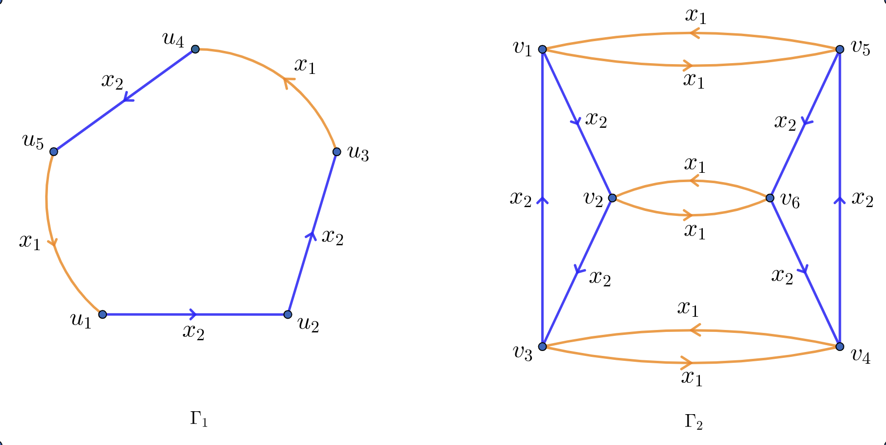
See the first one of Figure 5 where ω=x1​x2​x1​x22\omega=x_{1}x_{2}x_{1}x_{2}^{2}.

Refer to caption
Figure 5. Two X−X-labeled graphs
Construction (graph associated with (σ,τ)(\sigma,\tau)).

for any n≥1n\geq 1 and (σ,τ)∈ℰn(\sigma,\tau)\in\mathcal{E}_{n}, the associated X−X-labeled graph Γ​(σ,τ)\Gamma(\sigma,\tau) is constructed as follows,

  1. (1)

    firstly, there are 6​n6n vertices v1,…,v6​nv_{1},...,v_{6n};

  2. (2)

    for 1≤i≤6​n1\leq i\leq 6n, join viv_{i} and vσ​(i)v_{\sigma(i)} with a directed and labeled edge

    vi​→x1​vσ​(i);v_{i}\overset{x_{1}}{\to}v_{\sigma(i)};
  3. (3)

    for 1≤i≤6​n1\leq i\leq 6n, join viv_{i} and vτ​(i)v_{\tau(i)} with a directed and labeled edge

    vi​→x2​vτ​(i).v_{i}\overset{x_{2}}{\to}v_{\tau(i)}.

See the second one of Figure 5, where Γ2=Γ​(σ,τ)\Gamma_{2}=\Gamma(\sigma,\tau) for

σ=(15)​(26)​(34)​ and ​τ=(123)​(456).\sigma=(15)(26)(34)\text{ and }\tau=(123)(456).

By construction, it is easy to see that for any (σ,τ)∈ℰn​(n≥1)(\sigma,\tau)\in\mathcal{E}_{n}\ (n\geq 1), the X−X-labeled graph Γ​(σ,τ)\Gamma(\sigma,\tau) satisfies

  1. (1)

    the vertex set

    V​(Γ​(σ,τ))={v1,…,v6​n},V(\Gamma(\sigma,\tau))=\{v_{1},...,v_{6n}\},

    and for each vertex vi​(1≤i≤6​n)v_{i}\ (1\leq i\leq 6n), there are exactly four different edges based at it: two outgoing edges x1,x2x_{1},\ x_{2} and two incoming edges x1,x2x_{1},\ x_{2};

  2. (2)

    the edge set E​(Γ​(σ,τ))E(\Gamma(\sigma,\tau)) consists of cycles that are of the following two forms,

    vi​→x1​vσ​(i)​→x1​vi​ for ​1≤i≤6​nv_{i}\overset{x_{1}}{\to}v_{\sigma(i)}\overset{x_{1}}{\to}v_{i}\text{ for }1\leq i\leq 6n

    or

    vi​→x2​vτ​(i)​→x2​vτ2​(i)​→x2​vi​ for ​1≤i≤6​n.v_{i}\overset{x_{2}}{\to}v_{\tau(i)}\overset{x_{2}}{\to}v_{\tau^{2}(i)}\overset{x_{2}}{\to}v_{i}\text{ for }1\leq i\leq 6n.

Assume that GG and HH are both X−X-labeled graphs. Recall that as in [53], an X−X-labeled graph homomorphism

f:G→Hf:G\to H

is a pair of maps V​(G)→V​(H)V(G)\to V(H) and E​(G)→E​(H)E(G)\to E(H) such that

f​(u​→𝑒​v)=f​(u)​→𝑒​f​(v)f(u\overset{e}{\to}v)=f(u)\overset{e}{\to}f(v)

for any edge u​→𝑒​v∈E​(G)u\overset{e}{\to}v\in E(G) where u,v∈V​(G)u,v\in V(G) and e∈{x1,x2}e\in\{x_{1},x_{2}\}. It is called an X−X-labeled graph isomorphism if ff is a bijective X−X-labeled graph homomorphism. Now we give an example for an X−X-labeled graph homomorphism as follows: Let Γ1,Γ2\Gamma_{1},\Gamma_{2} be as in Figure 5, the graph homomorphism h:Γ1→Γ2h:\Gamma_{1}\to\Gamma_{2} is defined by

  1. (1)

    for 1≤i≤51\leq i\leq 5, set

    h​(ui)=vi;h(u_{i})=v_{i};
  2. (2)

    for 1≤i≤41\leq i\leq 4, set

    h​(ui​→ei​ui+1)=vi​→ei​vi+1,h(u_{i}\overset{e_{i}}{\to}u_{i+1})=v_{i}\overset{e_{i}}{\to}v_{i+1},

    where ei∈{x1,x2}e_{i}\in\{x_{1},x_{2}\} is uniquely determined by ii, and set

    h​(u5​→x1​u1)=v5​→x1​v1.h(u_{5}\overset{x_{1}}{\to}u_{1})=v_{5}\overset{x_{1}}{\to}v_{1}.

For this particular example, the X−X-labeled graph homomorphism hh defined above gives an embedding of Γ1\Gamma_{1} into Γ2\Gamma_{2}. However, in general, an X−X-labeled graph homomorphism hh defined on ΓX​(ω)\Gamma_{X}(\omega) is not necessarily an embedding.

3.2. Counting of fixed points

Assume ω=e1​e2​⋯​ek​(ei∈{x1±,x2±})\omega=e_{1}e_{2}\cdots e_{k}\ (e_{i}\in\{x_{1}^{\pm},x_{2}^{\pm}\}) is a reduced word in F2\textbf{F}_{2} and (σ,τ)∈ℰn​(n≥1)(\sigma,\tau)\in\mathcal{E}_{n}\ (n\geq 1), then Φ~​(σ,τ)​(ω)\tilde{\Phi}(\sigma,\tau)(\omega) is a permutation in S6​nS_{6n}. Denote by

fixω​(σ,τ)=#​{fixed points of thepermutation ​Φ~​(σ,τ)​(ω)}.\textnormal{fix}_{\omega}(\sigma,\tau)=\#\left\{\begin{matrix}\text{fixed points of the}\\ \text{permutation }\tilde{\Phi}(\sigma,\tau)(\omega)\end{matrix}\right\}.

Then

fixω:ℰn→ℤ≥0\textnormal{fix}_{\omega}:\mathcal{E}_{n}\to\mathbb{Z}^{\geq 0}

gives a random variable on ℰn\mathcal{E}_{n}. In this subsection, we will calculate its expected value

𝔼n​[fixω]=∑(σ,τ)∈ℰnfixω​(σ,τ)|ℰn|.\mathbb{E}_{n}[\textnormal{fix}_{\omega}]=\frac{\sum\limits_{(\sigma,\tau)\in\mathcal{E}_{n}}\textnormal{fix}_{\omega}(\sigma,\tau)}{|\mathcal{E}_{n}|}.

First of all, we have the following lemma.

Lemma 3.1.

Assume n≥1n\geq 1. Then for any reduced word ω∈F2\omega\in\textbf{F}_{2} and (σ,τ)∈ℰn(\sigma,\tau)\in\mathcal{E}_{n},

fixω​(σ,τ)=#​{X−labeled graph homomorphism f:ΓX​(ω)→Γ​(σ,τ)}.\displaystyle\textnormal{fix}_{\omega}(\sigma,\tau)=\#\left\{\begin{matrix}\text{$X-$labeled graph homomorphism }\\ f:\Gamma_{X}(\omega)\to\Gamma(\sigma,\tau)\end{matrix}\right\}.
Proof.

Assume ω=e1​e2​⋯​ek\omega=e_{1}e_{2}\cdots e_{k}, where ei∈{x1±,x2±}e_{i}\in\{x_{1}^{\pm},x_{2}^{\pm}\} and kk is the word length of ω\omega. For 1≤i≤k1\leq i\leq k, set

ξi={σ± if ​ei=x1±;τ± if ​ei=x2±.\xi_{i}=\begin{cases}\sigma^{\pm}&\text{ if }e_{i}=x_{1}^{\pm};\\ \tau^{\pm}&\text{ if }e_{i}=x_{2}^{\pm}.\end{cases}

Denote by ρ0=i​d\rho_{0}=id and

ρi=ξk−i+1​⋯​ξk.\rho_{i}=\xi_{k-i+1}\cdots\xi_{k}.

It is obvious that ρi∈S6​n​(0≤i≤k)\rho_{i}\in S_{6n}\ (0\leq i\leq k) and ρk=ξ1​⋯​ξk\rho_{k}=\xi_{1}\cdots\xi_{k}. Fix 1≤j≤6​n1\leq j\leq 6n. Since ρi+1​(j)=ξk−i​(ρi​(j))​(0≤i≤k−1)\rho_{i+1}(j)=\xi_{k-i}(\rho_{i}(j))\ (0\leq i\leq k-1), from the construction of Γ​(σ,τ)\Gamma(\sigma,\tau) there exists an edge

vρi​(j)​→ek−i​vρi+1​(j)v_{\rho_{i}(j)}\overset{e_{k-i}}{\to}v_{\rho_{i+1}(j)}

that joins vρi​(j)v_{\rho_{i}(j)} and vρi+1​(j)v_{\rho_{i+1}(j)} in Γ​(σ,τ)\Gamma(\sigma,\tau). It follows that there is a consecutive path PjP_{j}

vj​→ek​vρ1​(j)​→ek−1​⋯​→e2​vρk−1​(j)​→e1​vρk​(j)v_{j}\overset{e_{k}}{\to}v_{\rho_{1}(j)}\overset{e_{k-1}}{\to}\cdots\overset{e_{2}}{\to}v_{\rho_{k-1}(j)}\overset{e_{1}}{\to}v_{\rho_{k}(j)}

in Γ​(σ,τ)\Gamma(\sigma,\tau). Recall that ΓX​(ω)\Gamma_{X}(\omega) is a closed path

u1​→ek​u2​→ek−1​⋯​→e2​uk​→e1​u1.u_{1}\overset{e_{k}}{\to}u_{2}\overset{e_{k-1}}{\to}\cdots\overset{e_{2}}{\to}u_{k}\overset{e_{1}}{\to}u_{1}.

It follows that

ρk​(j)=j\displaystyle\rho_{k}(j)=j ⟺Pj​ is a closed path\displaystyle\Longleftrightarrow P_{j}\text{ is a closed path}
⟺there is a unique X−labeled graph homomorphismf:ΓX​(ω)→Γ​(σ,τ)​ such that f​(u1)=vj.\displaystyle\Longleftrightarrow\begin{matrix}\text{there is a unique $X-$labeled graph homomorphism}\\ f:\Gamma_{X}(\omega)\to\Gamma(\sigma,\tau)\text{ such that $f(u_{1})=v_{j}$.}\end{matrix}

Notice that

Φ~​(σ,τ)​(ω)=ρk=ξ1​ξ2​⋯​ξk,\tilde{\Phi}(\sigma,\tau)(\omega)=\rho_{k}=\xi_{1}\xi_{2}\cdots\xi_{k},

it follows that

fixω​(σ,τ)\displaystyle\textnormal{fix}_{\omega}(\sigma,\tau) =#​{fixed points of ​ρk}\displaystyle=\#\{\text{fixed points of }\rho_{k}\}
=#​{X−labeled graph homomorphism f:ΓX​(ω)→Γ​(σ,τ)}.\displaystyle=\#\left\{\begin{matrix}\text{$X-$labeled graph homomorphism }\\ f:\Gamma_{X}(\omega)\to\Gamma(\sigma,\tau)\end{matrix}\right\}.

The proof is complete. ∎

Example.

We consider an example (see Figure 5) for ω=x1​x2​x1​x22\omega=x_{1}x_{2}x_{1}x_{2}^{2} and

σ=(15)​(26)​(34),τ=(123)​(456).\sigma=(15)(26)(34),\ \tau=(123)(456).

Then it is direct to check that

Φ~​(σ,τ)​(ω)=i​d.\tilde{\Phi}(\sigma,\tau)(\omega)=id.

Hence for each 1≤i≤61\leq i\leq 6, ii is a fixed point of Φ~​(σ,τ)​(ω)\tilde{\Phi}(\sigma,\tau)(\omega). Meanwhile, for each 1≤i≤61\leq i\leq 6, there exists a unique X−X-labeled graph homomorphism hi:Γ1→Γ2h_{i}:\Gamma_{1}\to\Gamma_{2} such that hi​(u1)=vih_{i}(u_{1})=v_{i}.

From now on, we always assume that a word ω∈F2\omega\in\textbf{F}_{2} is of form

ω=x1​x2i1​⋯​x1​x2ik,\omega=x_{1}x_{2}^{i_{1}}\cdots x_{1}x_{2}^{i_{k}},

where k≥1k\geq 1 and ij∈{1,2}​(1≤j≤k)i_{j}\in\{1,2\}\ (1\leq j\leq k).

Construction (completion of ΓX​(ω)\Gamma_{X}(\omega)).

Based on ΓX​(ω)\Gamma_{X}(\omega), we construct an associated X−X-labeled graph ΓX​(ω)¯\overline{\Gamma_{X}(\omega)} as follows:

  1. (1)

    for any edge v1​→x1​v2v_{1}\overset{x_{1}}{\to}v_{2} in ΓX​(ω)\Gamma_{X}(\omega), add an edge v2​→x1​v1v_{2}\overset{x_{1}}{\to}v_{1} to ΓX​(ω)\Gamma_{X}(\omega);

  2. (2)

    for any consecutive edges

    u1​→x1​v1​→x2​v2​→x1​u2u_{1}\overset{x_{1}}{\to}v_{1}\overset{x_{2}}{\to}v_{2}\overset{x_{1}}{\to}u_{2}

    in ΓX​(ω)\Gamma_{X}(\omega), add a new vertex ww, and two new edges

    v2​→x2​w,ω​→x2​v1v_{2}\overset{x_{2}}{\to}w,\ \omega\overset{x_{2}}{\to}v_{1}

    to ΓX​(ω)\Gamma_{X}(\omega);

  3. (3)

    for any consecutive edges

    u1​→x1​v1​→x2​v2​→x2​v3​→x1​u2u_{1}\overset{x_{1}}{\to}v_{1}\overset{x_{2}}{\to}v_{2}\overset{x_{2}}{\to}v_{3}\overset{x_{1}}{\to}u_{2}

    in ΓX​(ω)\Gamma_{X}(\omega), add a new edge v3​→x2​v1v_{3}\overset{x_{2}}{\to}v_{1} to ΓX​(ω)\Gamma_{X}(\omega).

Refer to caption
Figure 6. Completion of ΓX​(ω)\Gamma_{X}(\omega)

One may see Figure 6 for an example of ω=x1​x2​x1​x22\omega=x_{1}x_{2}x_{1}x_{2}^{2}. It is obvious that for any (σ,τ)∈ℰn(\sigma,\tau)\in\mathcal{E}_{n} and X−X-labeled graph homomorphism f:ΓX​(ω)→Γ​(σ,τ)f:\Gamma_{X}(\omega)\to\Gamma(\sigma,\tau), ff could be uniquely extended to an X−X-labeled graph homomorphism

f¯:ΓX​(ω)¯→Γ​(σ,τ).\overline{f}:\overline{\Gamma_{X}(\omega)}\to\Gamma(\sigma,\tau).

Denote by

(5) F​(ω)={(g,Γ);g:ΓX​(ω)¯→Γ​ is a surjective X−labeledhomomorphism and Γ is a subgraph of Γ​(σ,τ) for some ​(σ,τ)∈ℰn​(n≥1)}.F(\omega)=\left\{(g,\Gamma);\ \begin{matrix}g:\overline{\Gamma_{X}(\omega)}\to\Gamma\text{ is a surjective $X-$labeled}\\ \text{homomorphism and $\Gamma$ is a subgraph }\\ \text{of $\Gamma(\sigma,\tau)$ for some }(\sigma,\tau)\in\mathcal{E}_{n}\ (n\geq 1)\end{matrix}\right\}.

For any two elements (g1,Γ1),(g2,Γ2)∈F​(ω)(g_{1},\Gamma_{1}),\ (g_{2},\Gamma_{2})\in F(\omega), we say that (g1,Γ1)(g_{1},\Gamma_{1}) and (g2,Γ2)(g_{2},\Gamma_{2}) are equivalent if there exists an X−X-labeled graph isomorphism ξ:Γ1→Γ2\xi:\Gamma_{1}\to\Gamma_{2} such that g2=ξ∘g1g_{2}=\xi\circ g_{1}, i.e. the following diagram commutes:

Γ1ΓX​(ω)¯Γ2ξg1g2.\hbox to68.96pt{\vbox to71.3pt{\pgfpicture\makeatletter\hbox{\hskip 34.4792pt\lower-35.65141pt\hbox to0.0pt{\pgfsys@beginscope\pgfsys@invoke{ }\definecolor{pgfstrokecolor}{rgb}{0,0,0}\pgfsys@color@rgb@stroke{0}{0}{0}\pgfsys@invoke{ }\pgfsys@color@rgb@fill{0}{0}{0}\pgfsys@invoke{ }\pgfsys@setlinewidth{\the\pgflinewidth}\pgfsys@invoke{ }\nullfont\hbox to0.0pt{\pgfsys@beginscope\pgfsys@invoke{ }{}{}{}{{}}\hbox{\hbox{{\pgfsys@beginscope\pgfsys@invoke{ }{{}{}{{{}}{{}}{{}}}{{{}}}{{}{}{{ {}{}}}{ {}{}} {{}{{}}}{{}{}}{}{{}{}} { }{{{{}}\pgfsys@beginscope\pgfsys@invoke{ }\pgfsys@transformcm{1.0}{0.0}{0.0}{1.0}{-34.4792pt}{-30.4917pt}\pgfsys@invoke{ }\hbox{\vbox{\halign{\pgf@matrix@init@row\pgf@matrix@step@column{\pgf@matrix@startcell#\pgf@matrix@endcell}&#\pgf@matrix@padding&&\pgf@matrix@step@column{\pgf@matrix@startcell#\pgf@matrix@endcell}&#\pgf@matrix@padding\cr\hfil\thinspace\hbox{{\pgfsys@beginscope\pgfsys@invoke{ }\pgfsys@invoke{ }\pgfsys@endscope{}}}&\thinspace\hfil&\hfil\qquad\hbox{{\pgfsys@beginscope\pgfsys@invoke{ }\pgfsys@invoke{ }\pgfsys@endscope{}}}&\thinspace\hfil&\hfil\hskip 27.67366pt\hbox{{\pgfsys@beginscope\pgfsys@invoke{ }{{}}\hbox{\hbox{{\pgfsys@beginscope\pgfsys@invoke{ }{{}{}{{ {}{}}}{ {}{}} {{}{{}}}{{}{}}{}{{}{}} { }{{{{}}\pgfsys@beginscope\pgfsys@invoke{ }\pgfsys@transformcm{1.0}{0.0}{0.0}{1.0}{-5.36807pt}{0.0pt}\pgfsys@invoke{ }\hbox{{\definecolor{pgfstrokecolor}{rgb}{0,0,0}\pgfsys@color@rgb@stroke{0}{0}{0}\pgfsys@invoke{ }\pgfsys@color@rgb@fill{0}{0}{0}\pgfsys@invoke{ }\hbox{${\Gamma_{1}}$} }}\pgfsys@invoke{ }\pgfsys@endscope}}} \pgfsys@invoke{ }\pgfsys@endscope}}} \pgfsys@invoke{ }\pgfsys@endscope}}&\quad\hfil\cr\vskip 13.50008pt\cr\hfil\thinspace\hbox{{\pgfsys@beginscope\pgfsys@invoke{ }\pgfsys@invoke{ }\pgfsys@endscope}}&\thinspace\hfil&\hfil\hskip 24.80559pt\hbox{{\pgfsys@beginscope\pgfsys@invoke{ }{{}}\hbox{\hbox{{\pgfsys@beginscope\pgfsys@invoke{ }{{}{}{{ {}{}}}{ {}{}} {{}{{}}}{{}{}}{}{{}{}} { }{{{{}}\pgfsys@beginscope\pgfsys@invoke{ }\pgfsys@transformcm{1.0}{0.0}{0.0}{1.0}{-2.5pt}{0.0pt}\pgfsys@invoke{ }\hbox{{\definecolor{pgfstrokecolor}{rgb}{0,0,0}\pgfsys@color@rgb@stroke{0}{0}{0}\pgfsys@invoke{ }\pgfsys@color@rgb@fill{0}{0}{0}\pgfsys@invoke{ }\hbox{${\overline{\Gamma_{X}(\omega)}}$} }}\pgfsys@invoke{ }\pgfsys@endscope}}} \pgfsys@invoke{ }\pgfsys@endscope}}} \pgfsys@invoke{ }\pgfsys@endscope}}&\quad\hfil&\hfil\qquad\hbox{{\pgfsys@beginscope\pgfsys@invoke{ }\pgfsys@invoke{ }\pgfsys@endscope}}&\thinspace\hfil\cr\vskip 13.50008pt\cr\hfil\thinspace\hbox{{\pgfsys@beginscope\pgfsys@invoke{ }\pgfsys@invoke{ }\pgfsys@endscope}}&\thinspace\hfil&\hfil\qquad\hbox{{\pgfsys@beginscope\pgfsys@invoke{ }\pgfsys@invoke{ }\pgfsys@endscope}}&\thinspace\hfil&\hfil\hskip 27.67366pt\hbox{{\pgfsys@beginscope\pgfsys@invoke{ }{{}}\hbox{\hbox{{\pgfsys@beginscope\pgfsys@invoke{ }{{}{}{{ {}{}}}{ {}{}} {{}{{}}}{{}{}}{}{{}{}} { }{{{{}}\pgfsys@beginscope\pgfsys@invoke{ }\pgfsys@transformcm{1.0}{0.0}{0.0}{1.0}{-5.36807pt}{0.0pt}\pgfsys@invoke{ }\hbox{{\definecolor{pgfstrokecolor}{rgb}{0,0,0}\pgfsys@color@rgb@stroke{0}{0}{0}\pgfsys@invoke{ }\pgfsys@color@rgb@fill{0}{0}{0}\pgfsys@invoke{ }\hbox{${\Gamma_{2}}$} }}\pgfsys@invoke{ }\pgfsys@endscope}}} \pgfsys@invoke{ }\pgfsys@endscope}}} \pgfsys@invoke{ }\pgfsys@endscope}}&\quad\hfil\cr}}}\pgfsys@invoke{ }\pgfsys@endscope}}}{{{{}}}{{}}{{}}{{}}}} \pgfsys@invoke{ }\pgfsys@endscope}}} {}{ {}{}{}}{}{ {}{}{}} {{{{{}}{ {}{}}{}{}{{}{}}}}}{}{{{{{}}{ {}{}}{}{}{{}{}}}}}{{}}{}{}{}{}{}{{{}{}}}{}{{}}{}{}{}{{{}{}}}\pgfsys@beginscope\pgfsys@invoke{ }\pgfsys@setlinewidth{\the\pgflinewidth}\pgfsys@invoke{ }{}{{ {\pgfsys@beginscope \pgfsys@setdash{\pgf@temp}{\the\pgf@x}\pgfsys@roundcap\pgfsys@roundjoin{} {}{}{} {}{}{} \pgfsys@moveto{-2.07988pt}{2.39986pt}\pgfsys@curveto{-1.69989pt}{0.95992pt}{-0.85313pt}{0.27998pt}{0.0pt}{0.0pt}\pgfsys@curveto{-0.85313pt}{-0.27998pt}{-1.69989pt}{-0.95992pt}{-2.07988pt}{-2.39986pt}\pgfsys@stroke\pgfsys@endscope}} }{}{}{{}}{}{}{{}}\pgfsys@moveto{24.80559pt}{19.79868pt}\pgfsys@lineto{24.80559pt}{-19.39871pt}\pgfsys@stroke\pgfsys@invoke{ }{{}{{}}{}{}{{}}{{{}}}}{{}{{}}{}{}{{}}{{{}}{{{}}{\pgfsys@beginscope\pgfsys@invoke{ }\pgfsys@transformcm{0.0}{-1.0}{1.0}{0.0}{24.80559pt}{-19.5987pt}\pgfsys@invoke{ }\pgfsys@invoke{ }\pgfsys@invoke{ }\pgfsys@endscope}}{{}}}}\hbox{\hbox{{\pgfsys@beginscope\pgfsys@invoke{ }{{}{}{{ {}{}}}{ {}{}} {{}{{}}}{{}{}}{}{{}{}} { }{{{{}}\pgfsys@beginscope\pgfsys@invoke{ }\pgfsys@transformcm{1.0}{0.0}{0.0}{1.0}{27.15836pt}{-1.75pt}\pgfsys@invoke{ }\hbox{{\definecolor{pgfstrokecolor}{rgb}{0,0,0}\pgfsys@color@rgb@stroke{0}{0}{0}\pgfsys@invoke{ }\pgfsys@color@rgb@fill{0}{0}{0}\pgfsys@invoke{ }\hbox{$\scriptstyle{\xi}$} }}\pgfsys@invoke{ }\pgfsys@endscope}}} \pgfsys@invoke{ }\pgfsys@endscope}}} \pgfsys@invoke{ }\pgfsys@endscope{}{ {}{}{}}{}{ {}{}{}} {{{{{}}{ {}{}}{}{}{{}{}}}}}{}{{{{{}}{ {}{}}{}{}{{}{}}}}}{{}}{}{}{}{}{}{{{}{}}}{}{{}}{}{}{}{{{}{}}}\pgfsys@beginscope\pgfsys@invoke{ }\pgfsys@setlinewidth{\the\pgflinewidth}\pgfsys@invoke{ }{}{}{}{}{{}}{}{}{{}}\pgfsys@moveto{-2.66808pt}{5.3483pt}\pgfsys@lineto{14.81905pt}{19.54657pt}\pgfsys@stroke\pgfsys@invoke{ }{{}{{}}{}{}{{}}{{{}}}}{{}{{}}{}{}{{}}{{{}}{{{}}{\pgfsys@beginscope\pgfsys@invoke{ }\pgfsys@transformcm{0.77634}{0.63033}{-0.63033}{0.77634}{14.97429pt}{19.67262pt}\pgfsys@invoke{ }\pgfsys@invoke{ }\pgfsys@invoke{ }\pgfsys@endscope}}{{}}}}\hbox{\hbox{{\pgfsys@beginscope\pgfsys@invoke{ }{{}{}{{ }}{ } {{}{{}}}{{}{}}{}{{}{}} { }{{{{}}\pgfsys@beginscope\pgfsys@invoke{ }\pgfsys@transformcm{1.0}{0.0}{0.0}{1.0}{-4.1773pt}{16.28734pt}\pgfsys@invoke{ }\hbox{{\definecolor{pgfstrokecolor}{rgb}{0,0,0}\pgfsys@color@rgb@stroke{0}{0}{0}\pgfsys@invoke{ }\pgfsys@color@rgb@fill{0}{0}{0}\pgfsys@invoke{ }\hbox{$\scriptstyle{g_{1}}$} }}\pgfsys@invoke{ }\pgfsys@endscope}}} \pgfsys@invoke{ }\pgfsys@endscope}}} \pgfsys@invoke{ }\pgfsys@endscope{}{ {}{}{}}{}{ {}{}{}} {{{{{}}{ {}{}}{}{}{{}{}}}}}{}{{{{{}}{ {}{}}{}{}{{}{}}}}}{{}}{}{}{}{}{}{{{}{}}}{}{{}}{}{}{}{{{}{}}}\pgfsys@beginscope\pgfsys@invoke{ }\pgfsys@setlinewidth{\the\pgflinewidth}\pgfsys@invoke{ }{}{}{}{}{{}}{}{}{{}}\pgfsys@moveto{-2.66808pt}{-5.95734pt}\pgfsys@lineto{14.62pt}{-19.8258pt}\pgfsys@stroke\pgfsys@invoke{ }{{}{{}}{}{}{{}}{{{}}}}{{}{{}}{}{}{{}}{{{}}{{{}}{\pgfsys@beginscope\pgfsys@invoke{ }\pgfsys@transformcm{0.78003}{-0.62573}{0.62573}{0.78003}{14.77599pt}{-19.95093pt}\pgfsys@invoke{ }\pgfsys@invoke{ }\pgfsys@invoke{ }\pgfsys@endscope}}{{}}}}\hbox{\hbox{{\pgfsys@beginscope\pgfsys@invoke{ }{{}{}{{}}{} {{}{{}}}{{}{}}{}{{}{}} { }{{{{}}\pgfsys@beginscope\pgfsys@invoke{ }\pgfsys@transformcm{1.0}{0.0}{0.0}{1.0}{-4.2761pt}{-18.38335pt}\pgfsys@invoke{ }\hbox{{\definecolor{pgfstrokecolor}{rgb}{0,0,0}\pgfsys@color@rgb@stroke{0}{0}{0}\pgfsys@invoke{ }\pgfsys@color@rgb@fill{0}{0}{0}\pgfsys@invoke{ }\hbox{$\scriptstyle{g_{2}}$} }}\pgfsys@invoke{ }\pgfsys@endscope}}} \pgfsys@invoke{ }\pgfsys@endscope}}} \pgfsys@invoke{ }\pgfsys@endscope \pgfsys@invoke{ }\pgfsys@endscope{}{}{}\hss}\pgfsys@discardpath\pgfsys@invoke{ }\pgfsys@endscope\hss}}\endpgfpicture}}.

Denote by

ℐ​(ω)= the set of all equivalent classes in F​(ω).\mathcal{I}(\omega)=\textit{ the set of all equivalent classes in $F(\omega)$.}

For any X−X-labeled graph homomorphism

f¯:ΓX​(ω)¯→Γ​(σ,τ),\overline{f}:\overline{\Gamma_{X}(\omega)}\to\Gamma(\sigma,\tau),

let Γ\Gamma be the image f¯​(ΓX​(ω)¯)⊂Γ​(σ,τ)\overline{f}\left(\overline{\Gamma_{X}(\omega)}\right)\subset\Gamma(\sigma,\tau) that induces a unique injective X−X-labeled homomorphism ι:Γ→Γ​(σ,τ)\iota:\Gamma\to\Gamma(\sigma,\tau) such that f¯=ι∘f¯\overline{f}=\iota\circ\overline{f}. Moreover, (f¯,f¯​(ΓX​(ω)¯))\left(\overline{f},\overline{f}\left(\overline{\Gamma_{X}(\omega)}\right)\right) corresponds to a unique element in ℐ​(ω)\mathcal{I}(\omega) denoted by (g,Γ)(g,\Gamma). Thus, together with Lemma 3.1, we have that for any fixed (σ,τ)∈ℰn(\sigma,\tau)\in\mathcal{E}_{n} and ω∈F2\omega\in\textbf{F}_{2},

(6) fixω​(σ,τ)\displaystyle\textnormal{fix}_{\omega}(\sigma,\tau) =#​{X−labeled graph homomorphism f:ΓX​(ω)→Γ​(σ,τ)}\displaystyle=\#\left\{\begin{matrix}\text{$X-$labeled graph homomorphism }\\ f:\Gamma_{X}(\omega)\to\Gamma(\sigma,\tau)\end{matrix}\right\}
=#​{X−labeled graph homomorphism f¯:ΓX​(ω)¯→Γ​(σ,τ)}\displaystyle=\#\left\{\begin{matrix}\text{$X-$labeled graph homomorphism }\\ \overline{f}:\overline{\Gamma_{X}(\omega)}\to\Gamma(\sigma,\tau)\end{matrix}\right\}
=∑(g,Γ)∈ℐ​(ω)#​{injective X−labeled graphhomomorphism ​ι:Γ→Γ​(σ,τ)}.\displaystyle=\sum\limits_{(g,\Gamma)\in\mathcal{I}(\omega)}\#\left\{\begin{matrix}\text{injective $X-$labeled graph}\\ \text{homomorphism }\iota:\Gamma\to\Gamma(\sigma,\tau)\end{matrix}\right\}.

3.2.1. Injective X−X-labeled graph homomorphisms

We first consider injective X−X-labeled graph homomorphisms. For any (σ,τ)∈ℰn​(n≥1)(\sigma,\tau)\in\mathcal{E}_{n}\ (n\geq 1) and (g,Γ)∈ℐ​(ω)(g,\Gamma)\in\mathcal{I}(\omega), set

𝒩Γ​(σ,τ)={injective X−labeled graph homomorphism ​ι:Γ→Γ​(σ,τ)}\mathcal{N}_{\Gamma}(\sigma,\tau)=\left\{\begin{matrix}\text{injective $X-$labeled graph }\\ \text{homomorphism }\iota:\Gamma\to\Gamma(\sigma,\tau)\end{matrix}\right\}

and

NΓ​(σ,τ)=#​𝒩Γ​(σ,τ).N_{\Gamma}(\sigma,\tau)=\#\mathcal{N}_{\Gamma}(\sigma,\tau).

Then

NΓ:ℰn→ℤ≥0N_{\Gamma}:\mathcal{E}_{n}\to\mathbb{Z}^{\geq 0}

is a random variable.

Definition.
  1. (1)

    An X−X-labeled graph H1H_{1} is called an x1−x_{1}-cycle if

    V​(H1)={u1,u2}​ and ​E​(H1)={u1​→x1​u2,u2​→x1​u1}.V(H_{1})=\{u_{1},u_{2}\}\text{ and }E(H_{1})=\{u_{1}\overset{x_{1}}{\to}u_{2},u_{2}\overset{x_{1}}{\to}u_{1}\}.
  2. (2)

    An X−X-labeled graph is called an x2−x_{2}-cycle if

    V​(H2)={u1,u2,u3}​ and ​E​(H2)={u1​→x2​u2,u2​→x2​u3,u3​→x2​u1}.V(H_{2})=\{u_{1},u_{2},u_{3}\}\text{ and }E(H_{2})=\{u_{1}\overset{x_{2}}{\to}u_{2},u_{2}\overset{x_{2}}{\to}u_{3},u_{3}\overset{x_{2}}{\to}u_{1}\}.

One may see Figure 7 for illustrations.

Refer to caption
Figure 7. Two cycles

Recall that the word ω∈F2\omega\in\textbf{F}_{2} is of form

ω=x1​x2i1​⋯​x1​x2ik\omega=x_{1}x_{2}^{i_{1}}\cdots x_{1}x_{2}^{i_{k}}

where k≥1,ij∈{1,2}​(1≤j≤k)k\geq 1,\ i_{j}\in\{1,2\}\ (1\leq j\leq k). For any element (g,Γ)∈ℐ​(ω)(g,\Gamma)\in\mathcal{I}(\omega), since gg maps xi−x_{i}-cycles in ΓX​(ω)¯\overline{\Gamma_{X}(\omega)} to xi−x_{i}-cycles in Γ​(σ,τ)\Gamma(\sigma,\tau) for i∈{1,2}i\in\{1,2\}, it follows that Γ=g​(ΓX​(ω)¯)\Gamma=g\left(\overline{\Gamma_{X}(\omega)}\right) is a union of certain x1−x_{1}-cycles and x2−x_{2}-cycles. Moreover, it satisfies that

  1. (1)

    for any vertex v∈V​(Γ)v\in V(\Gamma), it is contained in some an x2−x_{2}-cycle of Γ\Gamma;

  2. (2)

    for any x2−x_{2}-cycle of Γ\Gamma, at least two of its vertices are contained in some x1−x_{1}-cycles of Γ\Gamma.

Assume that Γ\Gamma has pp x1−x_{1}-cycles and qq x2−x_{2}-cycles. From condition (i) above, we have

|V​(Γ)|=3​q.|V(\Gamma)|=3q.

From condition (ii) above, we have p≥qp\geq q. See Figure 9 for an example in which p=4p=4 and q=3q=3. Define

η​(Γ)​=def​p−q≥0.\eta(\Gamma)\overset{\mathrm{def}}{=}p-q\geq 0.

Then we have the following lemma.

Proposition 3.2.

With the same assumptions as above, if |V​(Γ)|=o​(n12)|V(\Gamma)|=o\left(n^{\frac{1}{2}}\right), then we have

𝔼n​(NΓ)=1(6​n)η​(Γ)​(1+O​(|V​(Γ)|2n)),\mathbb{E}_{n}(N_{\Gamma})=\frac{1}{(6n)^{\eta(\Gamma)}}\left(1+O\left(\frac{|V(\Gamma)|^{2}}{n}\right)\right),

where the implied constant is independent of nn and Γ\Gamma.

Proof.

For any (σ,τ)∈ℰn(\sigma,\tau)\in\mathcal{E}_{n} and ι∈𝒩Γ​(σ,τ)\iota\in\mathcal{N}_{\Gamma}(\sigma,\tau), it naturally induces an injective map

ιv:V​(Γ)→{v1,…,v6​n}.\iota_{v}:V(\Gamma)\to\{v_{1},...,v_{6n}\}.

Since |V​(Γ)|=3​q|V(\Gamma)|=3q, it follows that there are

(7) ∏i=03​q−1(6​n−i)\displaystyle\prod\limits_{i=0}^{3q-1}(6n-i)

choices of such injective maps. Now we fix an injective map

ζ:V​(Γ)→{v1,…,v6​n}.\zeta:V(\Gamma)\to\{v_{1},...,v_{6n}\}.

Assume ι∈𝒩Γ​(σ,τ)\iota\in\mathcal{N}_{\Gamma}(\sigma,\tau) such that ιv=ζ\iota_{v}=\zeta. Then for any vertices u1≠u2∈V​(Γ)u_{1}\neq u_{2}\in V(\Gamma) and edge u1​→𝑒​u2∈E​(Γ)​(e∈{x1,x2})u_{1}\overset{e}{\to}u_{2}\in E(\Gamma)\ (e\in\{x_{1},x_{2}\}), there exists an edge

ζ​(u1)​→𝑒​ζ​(u2)∈E​(Γ​(σ,τ)).\zeta(u_{1})\overset{e}{\to}\zeta(u_{2})\in E(\Gamma(\sigma,\tau)).

Since ζ\zeta is injective and Γ\Gamma has pp x1−x_{1}-cycles and qq x2−x_{2}-cycles, it follows that there are pp x1−x_{1}-cycles and qq x2−x_{2}-cycles in Γ​(σ,τ)\Gamma(\sigma,\tau) that are determined by ζ\zeta. Recall that there are 3​n3n x1−x_{1}-cycles and 2​n2n x2−x_{2}-cycles in Γ​(σ,τ)\Gamma(\sigma,\tau), similar to the proof of Part (1) of Lemma 2.6 there are

(6​n−2​p)!(3​n−p)!​23​n−p×(6​n−3​q)!(2​n−q)!​32​n−q\frac{(6n-2p)!}{(3n-p)!2^{3n-p}}\times\frac{(6n-3q)!}{(2n-q)!3^{2n-q}}

choices to determine the remaining (3​n−p)(3n-p) x1−x_{1}-cycles and (2​n−q)(2n-q) x2−x_{2}-cycles. Hence we have

#​{ι;ι∈𝒩Γ​(σ,τ)​ for some ​(σ,τ)∈ℰn such that ​ιv=ζ}=(6​n−2​p)!(3​n−p)!​23​n−p×(6​n−3​q)!(2​n−q)!​32​n−q.\#\left\{\iota;\ \begin{matrix}\iota\in\mathcal{N}_{\Gamma}(\sigma,\tau)\text{ for some }(\sigma,\tau)\in\mathcal{E}_{n}\\ \text{ such that }\iota_{v}=\zeta\end{matrix}\right\}=\frac{(6n-2p)!}{(3n-p)!2^{3n-p}}\times\frac{(6n-3q)!}{(2n-q)!3^{2n-q}}.

This, together with (7) and Part (1)(1) of Lemma 2.6, implies that

(8) 𝔼n​(NΓ)\displaystyle\mathbb{E}_{n}(N_{\Gamma}) =∑(σ,τ)∈ℰnNΓ​(σ,τ)|ℰn|\displaystyle=\frac{\sum\limits_{(\sigma,\tau)\in\mathcal{E}_{n}}N_{\Gamma}(\sigma,\tau)}{|\mathcal{E}_{n}|}
=∏i=03​q−1(6​n−i)×(6​n−2​p)!(3​n−p)!​23​n−p×(6​n−3​q)!(2​n−q)!​32​n−q(6​n)!(3​n)!​23​n×(6​n)!(2​n)!​32​n\displaystyle=\frac{\prod\limits_{i=0}^{3q-1}(6n-i)\times\frac{(6n-2p)!}{(3n-p)!2^{3n-p}}\times\frac{(6n-3q)!}{(2n-q)!3^{2n-q}}}{\frac{(6n)!}{(3n)!2^{3n}}\times\frac{(6n)!}{(2n)!3^{2n}}}
=∏i=0p−1(3​n−i)×∏i=0q−1(2​n−i)∏i=02​p−1(6​n−i)×2p​3q.\displaystyle=\frac{\prod\limits_{i=0}^{p-1}(3n-i)\times\prod\limits_{i=0}^{q-1}(2n-i)}{\prod\limits_{i=0}^{2p-1}(6n-i)}\times 2^{p}3^{q}.

For any vertex v∈V​(Γ)v\in V(\Gamma), it is contained in at most one x1−x_{1}-cycle, and hence

(9) p≤|V​(Γ)|2.\displaystyle p\leq\frac{|V(\Gamma)|}{2}.

For k=o​(m12)k=o\left(m^{\frac{1}{2}}\right) and m>0m>0 large enough, it is known that

∏i=0k−1(m−i)=mk​(1+O​(k2m)).\prod\limits_{i=0}^{k-1}(m-i)=m^{k}\left(1+O\left(\frac{k^{2}}{m}\right)\right).

This together with (8) implies that

𝔼n​(NΓ)\displaystyle\mathbb{E}_{n}(N_{\Gamma}) =(3​n)p×(2​n)q(6​n)2​p×2p​3q​(1+O​(p2+q2n))\displaystyle=\frac{(3n)^{p}\times(2n)^{q}}{(6n)^{2p}}\times 2^{p}3^{q}\left(1+O\left(\frac{p^{2}+q^{2}}{n}\right)\right)
=1(6​n)η​(Γ)​(1+O​(|V​(Γ)|2n)),\displaystyle=\frac{1}{(6n)^{\eta(\Gamma)}}\left(1+O\left(\frac{|V(\Gamma)|^{2}}{n}\right)\right),

where we apply |V​(Γ)|=3​q|V(\Gamma)|=3q and (9) in the last equation. The proof is complete. ∎

The following lemma is the same as [44, Lemma 2.2] except an explicit expression for the constant C′C^{\prime} in [44, Lemma 2.2].

Lemma 3.3.

Let P,QP,\ Q be real polynomials of degree at most m∈ℕm\in\mathbb{N}, and let

Φ​(t)=P​(t)Q​(t).\Phi(t)=\frac{P(t)}{Q(t)}.

Assume that there is a constant C>1C>1 such that

(10) |P​(1n)|≤C​ and ​C−1≤Q​(1n)≤C\displaystyle\left|P\left(\frac{1}{n}\right)\right|\leq C\text{ and }C^{-1}\leq Q\left(\frac{1}{n}\right)\leq C

for all n∈ℕn\in\mathbb{N} with n≥(C​m)Cn\geq(Cm)^{C}. Denote by C′=4​C+5C^{\prime}=4C+5, then for all l≤C​ml\leq Cm,

supt∈[0,(C′​m)−C′]|Φ(l)​(t)|≤(C′​m)C′​l.\sup\limits_{t\in\left[0,(C^{\prime}m)^{-C^{\prime}}\right]}\left|\Phi^{(l)}(t)\right|\leq(C^{\prime}m)^{C^{\prime}l}.
Proof.

From the proof of [44, Lemma 2.2], we have

|Φ(l)​(t)|≤2l​(2​C)2​l+2​(2​C​m)4​C​l​l!\left|\Phi^{(l)}(t)\right|\leq 2^{l}(2C)^{2l+2}(2Cm)^{4Cl}l!

for any t∈[0,(2​C​m)−2​C−1]t\in[0,(2Cm)^{-2C-1}]. Hence for any l≤C​ml\leq Cm,

supt∈[0,(2​C​m)−2​C−1]|Φ(l)​(t)|\displaystyle\sup\limits_{t\in\left[0,(2Cm)^{-2C-1}\right]}\left|\Phi^{(l)}(t)\right| ≤2l​(2​C)2​l+2​(2​C​m)4​C​l​l!\displaystyle\leq 2^{l}(2C)^{2l+2}(2Cm)^{4Cl}l!
≤(2​C)2​l+2​(2​C​m)(4​C+1)​l\displaystyle\leq(2C)^{2l+2}(2Cm)^{(4C+1)l}
≤(2​C​m)(4​C+5)​l\displaystyle\leq(2Cm)^{(4C+5)l}

which implies that

supt∈[0,(C′​m)−C′]|Φ(l)​(t)|≤supt∈[0,(2​C​m)−2​C−1]|Φ(l)​(t)|≤(C′​m)C′​l.\sup\limits_{t\in\left[0,(C^{\prime}m)^{-C^{\prime}}\right]}\left|\Phi^{(l)}(t)\right|\leq\sup\limits_{t\in\left[0,(2Cm)^{-2C-1}\right]}\left|\Phi^{(l)}(t)\right|\leq(C^{\prime}m)^{C^{\prime}l}.

The proof is complete. ∎

Now we prove a more precise version of Proposition 3.2 for a fixed word ω∈F2\omega\in\textbf{F}_{2}.

Proposition 3.4.

Assume word ω=x1​x2i1​⋯​x1​x2ik∈F2\omega=x_{1}x_{2}^{i_{1}}\cdots x_{1}x_{2}^{i_{k}}\in\textbf{F}_{2}, where k≥1k\geq 1 and ij∈{1,2}​(1≤j≤k)i_{j}\in\{1,2\}\ (1\leq j\leq k). Also assume (g,Γ)∈ℐ​(ω)(g,\Gamma)\in\mathcal{I}(\omega), then

  1. (1)

    there exists a sequence {ai​(Γ)}i≥0⊂ℝ\{a_{i}(\Gamma)\}_{i\geq 0}\subset\mathbb{R} such that a0​(Γ)=1a_{0}(\Gamma)=1 and

    𝔼n​(NΓ)=1(6​n)η​(Γ)​∑i=0∞ai​(Γ)(6​n)i.\mathbb{E}_{n}(N_{\Gamma})=\frac{1}{(6n)^{\eta(\Gamma)}}\sum\limits_{i=0}^{\infty}\frac{a_{i}(\Gamma)}{(6n)^{i}}.
  2. (2)

    For all m≥2​km\geq 2k, l≤ml\leq m and 6​n≥(17​m)176n\geq(17m)^{17},

    |𝔼n​(NΓ)−1(6​n)η​(Γ)​∑i=0l−1ai​(Γ)(6​n)i|≤(17​m)17​ll!​(6​n)l+η​(Γ).\displaystyle\left|\mathbb{E}_{n}(N_{\Gamma})-\frac{1}{(6n)^{\eta(\Gamma)}}\sum\limits_{i=0}^{l-1}\frac{a_{i}(\Gamma)}{(6n)^{i}}\right|\leq\frac{(17m)^{17l}}{l!(6n)^{l+\eta(\Gamma)}}.
Proof.

(1). Assume that Γ\Gamma has pp x1−x_{1}-cycles and qq x2−x_{2}-cycles. Since (g,Γ)∈ℐ​(ω)(g,\Gamma)\in\mathcal{I}(\omega), we have

p,q≤k​ and ​|V​(Γ)|=3​q.p,q\leq k\text{ and }|V(\Gamma)|=3q.

From (8) in the proof of Lemma 3.2, we have

𝔼n​(NΓ)\displaystyle\mathbb{E}_{n}(N_{\Gamma}) =∏i=0p−1(3​n−i)×∏i=1q−1(2​n−i)∏i=02​p−1(6​n−i)×2p​3q\displaystyle=\frac{\prod\limits_{i=0}^{p-1}(3n-i)\times\prod\limits_{i=1}^{q-1}(2n-i)}{\prod\limits_{i=0}^{2p-1}(6n-i)}\times 2^{p}3^{q}
=1(6​n)η​(Γ)×∏i=0p−1(1−2​i6​n)×∏i=1q−1(1−3​i6​n)∏i=02​p−1(1−i6​n).\displaystyle=\frac{1}{(6n)^{\eta(\Gamma)}}\times\frac{\prod\limits_{i=0}^{p-1}\left(1-\frac{2i}{6n}\right)\times\prod\limits_{i=1}^{q-1}\left(1-\frac{3i}{6n}\right)}{\prod\limits_{i=0}^{2p-1}\left(1-\frac{i}{6n}\right)}.

Set

P​(t)=∏i=0p−1(1−2​i​t)×∏i=0q−1(1−3​i​t)​ and ​Q​(t)=∏i=02​p−1(1−i​t).P(t)=\prod\limits_{i=0}^{p-1}\left(1-2it\right)\times\prod\limits_{i=0}^{q-1}\left(1-3it\right)\text{ and }Q(t)=\prod\limits_{i=0}^{2p-1}\left(1-it\right).

Then the function PQ​(t)\frac{P}{Q}(t) could be represented as

PQ​(t)=∑i=0∞ai​(Γ)​ti\frac{P}{Q}(t)=\sum\limits_{i=0}^{\infty}a_{i}(\Gamma)t^{i}

for a sequence {ai​(Γ)}i≥0⊂ℝ\{a_{i}(\Gamma)\}_{i\geq 0}\subset\mathbb{R}. Hence

a0​(Γ)=PQ​(0)=1a_{0}(\Gamma)=\frac{P}{Q}(0)=1

and

𝔼n​(NΓ)=1(6​n)η​(Γ)×PQ​(16​n)=1(6​n)η​(Γ)​∑i=0∞ai​(Γ)(6​n)i.\mathbb{E}_{n}(N_{\Gamma})=\frac{1}{(6n)^{\eta(\Gamma)}}\times\frac{P}{Q}\left(\frac{1}{6n}\right)=\frac{1}{(6n)^{\eta(\Gamma)}}\sum\limits_{i=0}^{\infty}\frac{a_{i}(\Gamma)}{(6n)^{i}}.

(2). Assume m≥2​k≥2​pm\geq 2k\geq 2p. For 6​n≥(3​m)36n\geq(3m)^{3}, we have

|P​(16​n)|<3\left|P\left(\frac{1}{6n}\right)\right|<3

and

3\displaystyle 3 >Q​(16​n)=∏i=02​p−1(1−i6​n)\displaystyle>Q\left(\frac{1}{6n}\right)=\prod\limits_{i=0}^{2p-1}\left(1-\frac{i}{6n}\right)
≥∏i=02​p−1(1−i(3​m)3)≥∏i=02​p−1(1−1i2)>13.\displaystyle\geq\prod\limits_{i=0}^{2p-1}\left(1-\frac{i}{(3m)^{3}}\right)\geq\prod\limits_{i=0}^{2p-1}\left(1-\frac{1}{i^{2}}\right)>\frac{1}{3}.

Apply Lemma 3.3 to P​(t),Q​(t)P(t),\ Q(t) and C=3C=3, we have for any l≤3​ml\leq 3m,

supt∈[0,(17​m)−17]|(PQ)(l)​(t)|≤(17​m)17​l.\sup\limits_{t\in\left[0,(17m)^{-17}\right]}\left|\left(\frac{P}{Q}\right)^{(l)}(t)\right|\leq(17m)^{17l}.

It follows that for 6​n≥(17​m)176n\geq(17m)^{17} and l≤ml\leq m, there exists ξ∈[0,16​n]\xi\in[0,\frac{1}{6n}] such that

|𝔼n​(NΓ)−1(6​n)η​(Γ)​∑i=0l−1ai​(Γ)(6​n)i|\displaystyle\left|\mathbb{E}_{n}(N_{\Gamma})-\frac{1}{(6n)^{\eta(\Gamma)}}\sum\limits_{i=0}^{l-1}\frac{a_{i}(\Gamma)}{(6n)^{i}}\right| =1(6​n)η​(Γ)​|1l!​(6​n)l​(PQ)(l)​(ξ)|\displaystyle=\frac{1}{(6n)^{\eta(\Gamma)}}\left|\frac{1}{l!(6n)^{l}}\left(\frac{P}{Q}\right)^{(l)}(\xi)\right|
≤(17​m)17​ll!​(6​n)l+η​(Γ).\displaystyle\leq\frac{(17m)^{17l}}{l!(6n)^{l+\eta(\Gamma)}}.

The proof is complete. ∎

3.2.2. Surjective X−X-labeled graph homomorphisms

Now we consider surjective X−X-labeled graph homomorphisms. Assume ω∈F2\omega\in\textbf{F}_{2} is of form

ω=x1​x2i1​⋯​x1​x2ik=e1​e2​⋯​el,\omega=x_{1}x_{2}^{i_{1}}\cdots x_{1}x_{2}^{i_{k}}=e_{1}e_{2}\cdots e_{l},

where k≥1k\geq 1, ij∈{1,2}​(1≤j≤k)i_{j}\in\{1,2\}\ (1\leq j\leq k), 2​k≤l≤3​k2k\leq l\leq 3k, and ej∈{x1,x2}​(1≤j≤l)e_{j}\in\{x_{1},x_{2}\}\ (1\leq j\leq l). Recall that ΓX​(ω)\Gamma_{X}(\omega) is a closed path with its edges labeled as follows:

v1​→el​v2​→el−1​⋯​→e2​vl​→e1​v1.v_{1}\overset{e_{l}}{\to}v_{2}\overset{e_{l-1}}{\to}\cdots\overset{e_{2}}{\to}v_{l}\overset{e_{1}}{\to}v_{1}.

So for each 1≤j≤k1\leq j\leq k, x2ik+1−jx_{2}^{i_{k+1-j}} corresponds to certain consecutive edges in ΓX​(ω)\Gamma_{X}(\omega) of form

w1​→x1​w2​→x2​w3​→x1​w4​when ​ik+1−j=1,w_{1}\overset{x_{1}}{\to}w_{2}\overset{x_{2}}{\to}w_{3}\overset{x_{1}}{\to}w_{4}\ \text{when }i_{k+1-j}=1,

or

w1​→x1​w2​→x2​w3​→x2​w4​→x1​w5​when ​ik+1−j=2,w_{1}\overset{x_{1}}{\to}w_{2}\overset{x_{2}}{\to}w_{3}\overset{x_{2}}{\to}w_{4}\overset{x_{1}}{\to}w_{5}\ \text{when }i_{k+1-j}=2,

hence corresponds to an x2−x_{2}-cycle Δj\Delta_{j} in ΓX​(ω)¯\overline{\Gamma_{X}(\omega)}. For each 1≤j≤k1\leq j\leq k, there is an x1−x_{1}-cycle connecting Δj\Delta_{j} and Δj+1\Delta_{j+1} (set Δk+1=Δ1\Delta_{k+1}=\Delta_{1}).

Now we relabel the vertices in ΓX​(ω)¯\overline{\Gamma_{X}(\omega)} as follows: x2ik+1−j​(1≤j≤k)x_{2}^{i_{k+1-j}}\ (1\leq j\leq k) corresponds to an x2−x_{2}-cycle Δj\Delta_{j} of ΓX​(ω)¯\overline{\Gamma_{X}(\omega)}, label its vertices by v2​j−1,v2​jv_{2j-1},\ v_{2j} and uju_{j} so that

  1. (1)

    the two vertices v2​jv_{2j} and v2​j+1v_{2j+1} (1≤j≤k)(1\leq j\leq k) are joined by an x1−x_{1}-cycle of ΓX​(ω)¯\overline{\Gamma_{X}(\omega)}, (set v2​k+1=v1v_{2k+1}=v_{1});

  2. (2)

    the vertex uj​(1≤j≤k)u_{j}\ (1\leq j\leq k) is not contained in any x1−x_{1}-cycle of ΓX​(ω)¯\overline{\Gamma_{X}(\omega)}.

One may see Figure 8 for an example of ω=x1​x22​x1​x2​x1​x2\omega=x_{1}x_{2}^{2}x_{1}x_{2}x_{1}x_{2}.

Refer to caption
Figure 8. Relabel ΓX​(ω)¯\overline{\Gamma_{X}(\omega)} when ω=x1​x22​x1​x2​x1​x2\omega=x_{1}x_{2}^{2}x_{1}x_{2}x_{1}x_{2}

Now we give an algorithm to output all possible elements in ℐ​(ω)\mathcal{I}(\omega).

Algorithm (Algorithm for all outputs in ℐ​(ω)\mathcal{I}(\omega)).

First, we have the initial data 𝒜1=(Γ1,G1,f1,a1)\mathcal{A}_{1}=(\Gamma_{1},G_{1},f_{1},a_{1}), where

  • •

    Γ1\Gamma_{1} is the first x2−x_{2}-cycle Δ1\Delta_{1} in ΓX​(ω)¯\overline{\Gamma_{X}(\omega)};

  • •

    G1G_{1} is an x2−x_{2}-cycle w1​→x2​w2​→x2​w3​→x2​w1w_{1}\overset{x_{2}}{\to}w_{2}\overset{x_{2}}{\to}w_{3}\overset{x_{2}}{\to}w_{1};

  • •

    f1:Γ1→G1f_{1}:\Gamma_{1}\to G_{1} is the unique X−X-labeled graph homomorphism such that

    f​(v1)=w1;f(v_{1})=w_{1};
  • •

    a1=0a_{1}=0.

Suppose that we have 𝒜t=(Γt,Gt,ft,at)​(1≤t≤k−1)\mathcal{A}_{t}=(\Gamma_{t},G_{t},f_{t},a_{t})\ (1\leq t\leq k-1) after the (t−1)−(t-1)-th step. In the t−t-th step, we construct 𝒜t+1=(Γt+1,Gt+1,ft+1,at+1)\mathcal{A}_{t+1}=(\Gamma_{t+1},G_{t+1},f_{t+1},a_{t+1}) from 𝒜t\mathcal{A}_{t} as follows. Let Γt+1\Gamma_{t+1} be the subgraph of ΓX​(ω)¯\overline{\Gamma_{X}(\omega)} which consists of x2−x_{2}-cycles {Δ1,…,Δt+1}\{\Delta_{1},...,\Delta_{t+1}\} and x1−x_{1}-cycles that join Δi\Delta_{i} and Δi+1\Delta_{i+1} for all 1≤i≤t1\leq i\leq t, i.e. Γt+1\Gamma_{t+1} is obtained by adding an x1−x_{1}-cycle and an x2−x_{2}-cycle to Γt\Gamma_{t}. Then we construct Gt+1G_{t+1}. After relabeling ΓX​(ω)¯\overline{\Gamma_{X}(\omega)}, assume

ft​(v2​t)=wj,f_{t}(v_{2t})=w_{j},

where wjw_{j} is a vertex in GtG_{t},

  1. (1)

    if ωj\omega_{j} is not contained in any x1−x_{1}-cycle of GtG_{t}, then pick one of the following two operations randomly:

    • •

      Operation I: Take a new x2−x_{2}-cycle Δ\Delta

      w3​s+1​→x2​w3​s+2​→x2​w3​s+3​→x2​w3​s+1,w_{3s+1}\overset{x_{2}}{\to}w_{3s+2}\overset{x_{2}}{\to}w_{3s+3}\overset{x_{2}}{\to}w_{3s+1},

      where |V​(Gt)|=3​s|V(G_{t})|=3s. Let Gt+1G_{t+1} be the X−X-labeled graph which is obtained from GtG_{t} by adding an x2−x_{2}-cycle Δ\Delta and an x1−x_{1}-cycle that joins ωj\omega_{j} and ω3​s+1\omega_{3s+1}. Then ftf_{t} could be uniquely extended to an X−X-labeled graph homomorphism ft+1:Γt+1→Gt+1f_{t+1}:\Gamma_{t+1}\to G_{t+1}. Set at+1=ata_{t+1}=a_{t}.

    • •

      Operation II: Take a vertex ωl≠ωj∈V​(Gt)\omega_{l}\neq\omega_{j}\in V(G_{t}) such that wlw_{l} is not contained in any x1−x_{1}-cycle of GtG_{t}. Let Gt+1G_{t+1} be the X−X-labeled graph which is obtained from GtG_{t} by adding an x1−x_{1}-cycle that joins wjw_{j} and wlw_{l}. Then ftf_{t} could be uniquely extended to an X−X-labeled graph homomorphism ft+1:Γt+1→Gt+1f_{t+1}:\Gamma_{t+1}\to G_{t+1}. Set at+1=at+1a_{t+1}=a_{t}+1.

  2. (2)

    If ωj\omega_{j} is contained in an x1−x_{1}-cycle of GtG_{t}, we then set Gt+1=GtG_{t+1}=G_{t}, and ftf_{t} could be uniquely extended to an X−X-labeled graph homomorphism

    ft+1:Γt+1→Gt+1.f_{t+1}:\Gamma_{t+1}\to G_{t+1}.

    Set at+1=ata_{t+1}=a_{t}.

After the (k−1)−(k-1)-th step, we obtain 𝒜k=(Γk,Gk,fk,ak)\mathcal{A}_{k}=(\Gamma_{k},G_{k},f_{k},a_{k}). Now we finish the last step. Assume

fk​(v2​k)=wr,f_{k}(v_{2k})=w_{r},

where wrw_{r} is a vertex of GkG_{k}, there are three possible outputs as follows:

  1. (1)

    If neither wrw_{r} nor w1w_{1} is contained in any x1−x_{1}-cycle of GkG_{k}, denote by Gk+1G_{k+1} the X−X-labeled graph obtained from GkG_{k} by adding an x1−x_{1}-cycle that joins ωr\omega_{r} and ω1\omega_{1} (i.e. we make Operation II). Then fkf_{k} could be uniquely extended to a surjective X−X-labeled graph homomorphism fk+1:ΓX​(ω)¯→Gk+1f_{k+1}:\overline{\Gamma_{X}(\omega)}\to G_{k+1}. Set ak+1=ak+1a_{k+1}=a_{k}+1.

  2. (2)

    If wrw_{r} and w1w_{1} are contained in the same x1−x_{1}-cycle of GkG_{k}, set Gk+1=GkG_{k+1}=G_{k}. Then fkf_{k} could be uniquely extended to a surjective X−X-labeled graph homomorphism fk+1:ΓX​(ω)¯→Gk+1f_{k+1}:\overline{\Gamma_{X}(\omega)}\to G_{k+1}. Set ak+1=aka_{k+1}=a_{k}.

  3. (3)

    For all remaining cases, set 𝒜k+1=∅.\mathcal{A}_{k+1}=\emptyset.

Finally, we obtain 𝒜k+1=(ΓX​(ω)¯,Gk+1,fk+1,ak+1)\mathcal{A}_{k+1}=\left(\overline{\Gamma_{X}(\omega)},G_{k+1},f_{k+1},a_{k+1}\right) or ∅\emptyset.

Remark.

It is clear that for any output 𝒜k+1=(ΓX​(ω)¯,Gk+1,fk+1,ak+1)\mathcal{A}_{k+1}=\left(\overline{\Gamma_{X}(\omega)},G_{k+1},f_{k+1},a_{k+1}\right) of ω\omega, we have

ak+1≤k.a_{k+1}\leq k.
Refer to caption
Figure 9. An output for ω=x1​x2​x1​x22​x1​x2​x1​x2​x1​x22\omega=x_{1}x_{2}x_{1}x_{2}^{2}x_{1}x_{2}x_{1}x_{2}x_{1}x_{2}^{2}
Example.

Now we consider an example for ω=x1​x2​x1​x22​x1​x2​x1​x2​x1​x22\omega=x_{1}x_{2}x_{1}x_{2}^{2}x_{1}x_{2}x_{1}x_{2}x_{1}x_{2}^{2} containing all possible operations above (see Figure 9). Assume that the vertices of ΓX​(ω)¯\overline{\Gamma_{X}(\omega)} have been relabeled. First, we have 𝒜1=(Γ1,G1,f1,a1=0)\mathcal{A}_{1}=(\Gamma_{1},G_{1},f_{1},a_{1}=0), where the X−X-labeled graph homomorphism f1f_{1} is uniquely determined by

f1​(v1)=w1,f1​(v2)=w3,f1​(u1)=w2.f_{1}(v_{1})=w_{1},\ f_{1}(v_{2})=w_{3},\ f_{1}(u_{1})=w_{2}.

Step 1: w3w_{3} is not contained in any x1−x_{1}-cycle of G1G_{1}. Make Operation I, we obtain a graph G2G_{2} from G1G_{1} by adding a new x2−x_{2}-cycle

w4​→x2​w5​→x2​w6​→x2​w4,w_{4}\overset{x_{2}}{\to}w_{5}\overset{x_{2}}{\to}w_{6}\overset{x_{2}}{\to}w_{4},

and joining w3w_{3} and w4w_{4} with an x1−x_{1}-cycle. Set a2=0a_{2}=0. The X−X-labeled graph homomorphism f1f_{1} could be uniquely extended to f2:Γ2→G2f_{2}:\Gamma_{2}\to G_{2} such that

f2​(v3)=w4,f2​(v4)=w5,f2​(u2)=w6.f_{2}(v_{3})=w_{4},\ f_{2}(v_{4})=w_{5},\ f_{2}(u_{2})=w_{6}.

Step 2: w5w_{5} is not contained in any x1−x_{1}-cycle of G2G_{2}. Make Operation II, we obtain a graph G3G_{3} from G2G_{2} by joining w5w_{5} and w2w_{2} with an x1−x_{1}-cycle (we remark here that this is not the unique way, e.g. one may add an x1−x_{1}-cycle between w5w_{5} and w1w_{1}). Set a3=1a_{3}=1. The X−X-labeled graph homomorphism f2f_{2} could be uniquely extended to f3:Γ3→G3f_{3}:\Gamma_{3}\to G_{3} such that

f3​(v5)=w2,f3​(v6)=w3,f3​(u3)=w1.f_{3}(v_{5})=w_{2},\ f_{3}(v_{6})=w_{3},\ f_{3}(u_{3})=w_{1}.

Step 3: w3w_{3} is contained in an x1−x_{1}-cycle of G3G_{3}. Set G4=G3G_{4}=G_{3} and a4=1a_{4}=1. The X−X-labeled graph homomorphism f3f_{3} could be uniquely extended to f4:Γ4→G4f_{4}:\Gamma_{4}\to G_{4} such that

f4​(v7)=w4,f4​(v8)=w6,f4​(u4)=w5.f_{4}(v_{7})=w_{4},\ f_{4}(v_{8})=w_{6},\ f_{4}(u_{4})=w_{5}.

Step 4: w6w_{6} is not contained in any x1−x_{1}-cycle of G4G_{4}. Make Operation I, we obtain a graph G5G_{5} from G4G_{4} by adding a new x2−x_{2}-cycle

w7​→x2​w8​→x2​w9​→x2​w7,w_{7}\overset{x_{2}}{\to}w_{8}\overset{x_{2}}{\to}w_{9}\overset{x_{2}}{\to}w_{7},

and joining w6w_{6} and w7w_{7} with an x1−x_{1}-cycle. Set a5=1a_{5}=1. The X−X-labeled graph homomorphism f4f_{4} could be uniquely extended to f5:Γ5→G5f_{5}:\Gamma_{5}\to G_{5} such that

f5​(v9)=w7,f5​(v10)=w8,f5​(u5)=w9.f_{5}(v_{9})=w_{7},\ f_{5}(v_{10})=w_{8},\ f_{5}(u_{5})=w_{9}.

Step 5: Neither w8w_{8} nor w1w_{1} is contained in any x1−x_{1}-cycle of G5G_{5}. We obtain a graph G6G_{6} from G5G_{5} by joining w8w_{8} and w1w_{1} with an x1−x_{1}-cycle. Set a6=2a_{6}=2. The X−X-labeled graph homomorphism f5f_{5} could be uniquely extended to

f6:ΓX​(ω)¯→G6.f_{6}:\overline{\Gamma_{X}(\omega)}\to G_{6}.

Finally, we get an output

𝒜6=(ΓX​(ω)¯,G6,f6,2).\mathcal{A}_{6}=\left(\overline{\Gamma_{X}(\omega)},G_{6},f_{6},2\right).

Recall that ω∈F2\omega\in\textbf{F}_{2} could be represented as

ω=x1​x2i1​⋯​x1​x2ik,\omega=x_{1}x_{2}^{i_{1}}\cdots x_{1}x_{2}^{i_{k}},

where k≥1k\geq 1 and ij∈{1,2}​(1≤j≤k)i_{j}\in\{1,2\}\ (1\leq j\leq k). Denote by

𝔇​(ω)={all possible output data 𝒜=(ΓX​(ω)¯,G,f,a) for ​ω}.\mathfrak{D}(\omega)=\left\{\text{all possible output data $\mathcal{A}=\left(\overline{\Gamma_{X}(\omega)},G,f,a\right)$ for }\omega\right\}.

For any 𝒜=(ΓX​(ω)¯,G,f,a)\mathcal{A}=\left(\overline{\Gamma_{X}(\omega)},G,f,a\right) and 𝒜′=(ΓX​(ω)¯,G′,f′,a′)\mathcal{A}^{\prime}=\left(\overline{\Gamma_{X}(\omega)},G^{\prime},f^{\prime},a^{\prime}\right) in 𝔇​(ω)\mathfrak{D}(\omega), we say 𝒜\mathcal{A} and 𝒜′\mathcal{A}^{\prime} are equivalent if (f,G)(f,G) and (f′,G′)(f^{\prime},G^{\prime}) are equivalent in F​(ω)F(\omega) given by (5). Denote by

𝔉​(ω)= the set of all equivalent classes in ​𝔇​(ω)\mathfrak{F}(\omega)=\text{ the set of all equivalent classes in }\mathfrak{D}(\omega)

and

𝔉h(ω)={𝒜=(ΓX​(ω)¯,G,f,a)∈𝔉(ω);a=h} for h≥1.\mathfrak{F}_{h}(\omega)=\left\{\mathcal{A}=\left(\overline{\Gamma_{X}(\omega)},G,f,a\right)\in\mathfrak{F}(\omega);\ a=h\right\}\text{ for }h\geq 1.

Then we have the following two lemmas.

Lemma 3.5.

Assume h≥1h\geq 1 and ω∈F2\omega\in\textbf{F}_{2} is of form

ω=x1​x2i1​⋯​x1​x2ik,\omega=x_{1}x_{2}^{i_{1}}\cdots x_{1}x_{2}^{i_{k}},

where k≥1k\geq 1 and ij∈{1,2}​(1≤j≤k)i_{j}\in\{1,2\}\ (1\leq j\leq k), then we have

  1. (1)

    |𝔉h​(ω)|≤k2​h−1|\mathfrak{F}_{h}(\omega)|\leq k^{2h-1}.

  2. (2)

    Assume 𝒜=(ΓX​(ω)¯,G,f,h)∈𝔉h​(ω)\mathcal{A}=\left(\overline{\Gamma_{X}(\omega)},G,f,h\right)\in\mathfrak{F}_{h}(\omega), then

    η​(G)=h−1.\eta(G)=h-1.
Proof.

Recall from the algorithm above the initial data 𝒜1=(Γ1,G1,f1,a1)\mathcal{A}_{1}=(\Gamma_{1},G_{1},f_{1},a_{1}), and after the t−t-th step (1≤t≤k1\leq t\leq k), we obtain

𝒜t+1=(Γt+1,Gt+1,ft+1,at+1).\mathcal{A}_{t+1}=(\Gamma_{t+1},G_{t+1},f_{t+1},a_{t+1}).

Consider the processes that produce elements in 𝔉h​(ω)\mathfrak{F}_{h}(\omega). During such processes, we make Operation II exactly hh times. For any 1≤t≤k−11\leq t\leq k-1,

  1. (1)

    if at the t−t-th step, we make Operation II, then there are at most kk different choices for constructing a new graph Gt+1G_{t+1} from GtG_{t};

  2. (2)

    otherwise, the new graph Gt+1G_{t+1} is uniquely determined by GtG_{t}.

Moreover, there exists some 1≤t0≤k1\leq t_{0}\leq k such that at the t0−t_{0}-th step, we make Operation II and join w1w_{1} with some wiw_{i} by an x1−x_{1}-cycle. Since there are at most (kh)\binom{k}{h} different choices to determine the remaining hh steps at which we make Operation II, it follows that

|𝔉h​(ω)|≤(kh)×kh−1≤k2​h−1,\displaystyle|\mathfrak{F}_{h}(\omega)|\leq\binom{k}{h}\times k^{h-1}\leq k^{2h-1},

which yields the desired bound in Part (1)(1).

Now we prove Part (2)(2). Consider a process that outputs 𝒜\mathcal{A}, i.e. 𝒜=𝒜k+1\mathcal{A}=\mathcal{A}_{k+1}. Also, assume that the graph GtG_{t} has ptp_{t} x1−x_{1}-cycles and qtq_{t} x2−x_{2}-cycles for 1≤t≤(k+1)1\leq t\leq(k+1). Denote by

ηt=pt−qt.\eta_{t}=p_{t}-q_{t}.

By the definition of our algorithm, it is clear that

p1=0,q1=1​ and ​η1=−1.p_{1}=0,\ q_{1}=1\text{ and }\eta_{1}=-1.

For any 1≤t≤k−11\leq t\leq k-1,

  1. (1)

    if at the t−t-th step, we make Operation I, then

    pt+1=pt+1,qt+1=qt+1​ and ​ηt+1=ηt;p_{t+1}=p_{t}+1,\ q_{t+1}=q_{t}+1\text{ and }\eta_{t+1}=\eta_{t};
  2. (2)

    if at the t−t-th step, we make Operation II, then

    pt+1=pt+1,qt+1=qt​ and ​ηt+1=ηt+1;p_{t+1}=p_{t}+1,\ q_{t+1}=q_{t}\text{ and }\eta_{t+1}=\eta_{t}+1;
  3. (3)

    for the remaining case, we have

    pt+1=pt,qt+1=qt​ and ​ηt+1=ηt.p_{t+1}=p_{t},\ q_{t+1}=q_{t}\text{ and }\eta_{t+1}=\eta_{t}.

Consider the k−k-th step, i.e. the final step,

  1. (a)

    if neither wjw_{j} nor w1w_{1} is contained in any x1−x_{1}-cycle of GkG_{k}, then we make Operation II and

    pk+1=pk+1,qk+1=qk​ and ​ηk+1=ηk+1;p_{k+1}=p_{k}+1,\ q_{k+1}=q_{k}\text{ and }\eta_{k+1}=\eta_{k}+1;
  2. (b)

    if wjw_{j} and w1w_{1} are contained in the same x1−x_{1}-cycle of GkG_{k}, then

    pk+1=pk,qk+1=qk​ and ​ηk+1=ηk.p_{k+1}=p_{k},\ q_{k+1}=q_{k}\text{ and }\eta_{k+1}=\eta_{k}.

Since we make Operation II exactly hh times, it follows that η​(G)=ηk+1=h−1\eta(G)=\eta_{k+1}=h-1.

The proof is complete. ∎

Lemma 3.6.

Assume ω∈F2\omega\in\textbf{F}_{2} is of form

ω=x1​x2i1​⋯​x1​x2ik,\omega=x_{1}x_{2}^{i_{1}}\cdots x_{1}x_{2}^{i_{k}},

where k≥1k\geq 1 and ij∈{1,2}​(1≤j≤k)i_{j}\in\{1,2\}\ (1\leq j\leq k). Assume 𝒜=(ΓX​(ω)¯,G,f,1)∈𝔉1​(ω)\mathcal{A}=\left(\overline{\Gamma_{X}(\omega)},G,f,1\right)\in\mathfrak{F}_{1}(\omega), then

G=ΓX​(ν)¯,G=\overline{\Gamma_{X}(\nu)},

where ν∈F2\nu\in\textbf{F}_{2} is a reduced word such that ω=νq\omega=\nu^{q} for some q≥1q\geq 1.

Proof.

Consider a process that outputs 𝒜\mathcal{A}, i.e. 𝒜=𝒜k+1\mathcal{A}=\mathcal{A}_{k+1}. We assume after the t−t-th (0≤t≤k)(0\leq t\leq k) step, we obtain

𝒜t+1=(Γt+1,Gt+1,ft+1,at+1),\mathcal{A}_{t+1}=(\Gamma_{t+1},G_{t+1},f_{t+1},a_{t+1}),

and ft+1​(v2​t+2)=wjt+1∈V​(Gt+1)f_{t+1}(v_{2t+2})=w_{j_{t+1}}\in V(G_{t+1}). Since

𝒜=(ΓX​(ω)¯,G,f,1)∈𝔉1​(ω),\mathcal{A}=\left(\overline{\Gamma_{X}(\omega)},G,f,1\right)\in\mathfrak{F}_{1}(\omega),

we only make one Operation II at some s−s-th step where 1≤s≤k1\leq s\leq k. Now we claim that at the s−s-th step, wjsw_{j_{s}} and w1w_{1} is joined by an x1−x_{1}-cycle. Otherwise, we find that wjsw_{j_{s}} and wlw_{l} is joined by an x1−x_{1}-cycle for some l≠1l\neq 1, then w1w_{1} is not contained in any x1−x_{1}-cycle of GkG_{k}, and hence we have to join w1w_{1} and some vertex in GkG_{k} with an x1−x_{1}-cycle at the k−k-th step. It follows that we make Operation II at least twice, which leads to a contradiction. Then we have

  1. (1)

    for 1≤t≤s−11\leq t\leq s-1, we make Operation I at each t−t-th step (i.e Gt+1G_{t+1} is obtained from GtG_{t} by adding a new x1−x_{1}-cycle and a new x2−x_{2}-cycle);

  2. (2)

    for s+1≤t≤ks+1\leq t\leq k, wjtw_{j_{t}} is contained in an x1−x_{1}-cycle of GtG_{t}. Hence Gt=Gt+1G_{t}=G_{t+1}.

Take

ν=x1​x2ik+1−s​⋯​x1​x2ik,\nu=x_{1}x_{2}^{i_{k+1-s}}\cdots x_{1}x_{2}^{i_{k}},

then from conditions (i) and (ii) above, we have

G=Gs+1=ΓX​(ν)¯​ and ​ω=νqG=G_{s+1}=\overline{\Gamma_{X}(\nu)}\textnormal{ \ and \ }\omega=\nu^{q}

for some q≥1q\geq 1. The proof is complete. ∎

3.2.3. Number of fixed points

In this subsection, we calculate the expected value 𝔼n​[fixω]\mathbb{E}_{n}[\textnormal{fix}_{\omega}] for any fixed ω∈F2\omega\in\textbf{F}_{2}. We prove two propositions.

Proposition 3.7.

Assume ω∈F2\omega\in\textbf{F}_{2} is a fixed word of form

ω=x1​x2i1​⋯​x1​x2ik,\omega=x_{1}x_{2}^{i_{1}}\cdots x_{1}x_{2}^{i_{k}},

where k≥1k\geq 1 and ij∈{1,2}​(1≤j≤k)i_{j}\in\{1,2\}\ (1\leq j\leq k). Then there exist a sequence {vi​(ω)}i≥0⊂ℝ\{v_{i}(\omega)\}_{i\geq 0}\subset\mathbb{R} such that

|𝔼n​[fixω]−∑i=0m−1vi​(ω)(6​n)i|≤(18​m)18​m(6​n)m\left|\mathbb{E}_{n}\left[\textnormal{fix}_{\omega}\right]-\sum\limits_{i=0}^{m-1}\frac{v_{i}(\omega)}{(6n)^{i}}\right|\leq\frac{(18m)^{18m}}{(6n)^{m}}

for all m≥2​km\geq 2k and 6​n≥18​m186n\geq 18m^{18}.

Proof.

Assume m≥2​km\geq 2k and 6​n≥17​m176n\geq 17m^{17}. From (6) we know that

𝔼n​[fixω]=∑(g,Γ)∈ℐ​(ω)𝔼n​(NΓ).\mathbb{E}_{n}\left[\textnormal{fix}_{\omega}\right]=\sum\limits_{(g,\Gamma)\in\mathcal{I}(\omega)}\mathbb{E}_{n}(N_{\Gamma}).

Then we have

(11) |𝔼n​[fixω]−∑(g,Γ)∈ℐ​(ω)1(6​n)η​(Γ)​∑i=0m−1−η​(Γ)ai​(Γ)(6​n)i|\displaystyle\ \ \ \ \left|\mathbb{E}_{n}\left[\textnormal{fix}_{\omega}\right]-\sum\limits_{(g,\Gamma)\in\mathcal{I}(\omega)}\frac{1}{(6n)^{\eta(\Gamma)}}\sum\limits_{i=0}^{m-1-\eta(\Gamma)}\frac{a_{i}(\Gamma)}{(6n)^{i}}\right|
=|∑(g,Γ)∈ℐ​(ω)𝔼n​(NΓ)−∑(g,Γ)∈ℐ​(ω)1(6​n)η​(Γ)​∑i=0m−1−η​(Γ)ai​(Γ)(6​n)i|\displaystyle=\left|\sum\limits_{(g,\Gamma)\in\mathcal{I}(\omega)}\mathbb{E}_{n}(N_{\Gamma})-\sum\limits_{(g,\Gamma)\in\mathcal{I}(\omega)}\frac{1}{(6n)^{\eta(\Gamma)}}\sum\limits_{i=0}^{m-1-\eta(\Gamma)}\frac{a_{i}(\Gamma)}{(6n)^{i}}\right|
≤∑(g,Γ)∈ℐ​(ω)|𝔼n​(NΓ)−1(6​n)η​(Γ)​∑i=0m−1−η​(Γ)ai​(Γ)(6​n)i|,\displaystyle\leq\sum\limits_{(g,\Gamma)\in\mathcal{I}(\omega)}\left|\mathbb{E}_{n}(N_{\Gamma})-\frac{1}{(6n)^{\eta(\Gamma)}}\sum\limits_{i=0}^{m-1-\eta(\Gamma)}\frac{a_{i}(\Gamma)}{(6n)^{i}}\right|,

where in the summations above, we set

∑i=0m−1−η​(Γ)ai​(Γ)(6​n)i=0\sum\limits_{i=0}^{m-1-\eta(\Gamma)}\frac{a_{i}(\Gamma)}{(6n)^{i}}=0

for the case η​(Γ)≥m\eta(\Gamma)\geq m. Now applying Proposition 3.4 to (g,Γ)∈ℐ​(ω)(g,\Gamma)\in\mathcal{I}(\omega) and l=m−η​(Γ)l=m-\eta(\Gamma), we have

(12) |𝔼n​(NΓ)−1(6​n)η​(Γ)​∑i=0m−1−η​(Γ)ai​(Γ)(6​n)i|≤(17​m)17​(m−η​(Γ))(6​n)m.\displaystyle\left|\mathbb{E}_{n}(N_{\Gamma})-\frac{1}{(6n)^{\eta(\Gamma)}}\sum\limits_{i=0}^{m-1-\eta(\Gamma)}\frac{a_{i}(\Gamma)}{(6n)^{i}}\right|\leq\frac{(17m)^{17(m-\eta(\Gamma))}}{(6n)^{m}}.

From Lemma 3.5 we have for h≥0h\geq 0,

#​{(g,Γ)∈ℐ​(ω);η​(Γ)=h}=|𝔉h+1​(ω)|≤k2​h+1.\#\{(g,\Gamma)\in\mathcal{I}(\omega);\ \eta(\Gamma)=h\}=|\mathfrak{F}_{h+1}(\omega)|\leq k^{2h+1}.

It then follows that for m≥2​km\geq 2k and 6​n≥18​m186n\geq 18m^{18},

(13) ∑(g,Γ)∈ℐ​(ω)(17​m)17​(m−η​(Γ))(6​n)m\displaystyle\sum\limits_{(g,\Gamma)\in\mathcal{I}(\omega)}\frac{(17m)^{17(m-\eta(\Gamma))}}{(6n)^{m}} =∑h=0∞∑(g,Γ)∈ℐ​(ω)η​(Γ)=h(17​m)17​(m−h)(6​n)m\displaystyle=\sum\limits_{h=0}^{\infty}\sum\limits\limits_{\begin{subarray}{c}(g,\Gamma)\in\mathcal{I}(\omega)\\ \eta(\Gamma)=h\end{subarray}}\frac{(17m)^{17(m-h)}}{(6n)^{m}}
≤∑h=0∞(17​m)17​(m−h)(6​n)m×k2​h+1\displaystyle\leq\sum\limits_{h=0}^{\infty}\frac{(17m)^{17(m-h)}}{(6n)^{m}}\times k^{2h+1}
≤(18​m)18​m(6​n)m.\displaystyle\leq\frac{(18m)^{18m}}{(6n)^{m}}.

Take

(14) vj​(ω)=∑(g,Γ)∈ℐ​(ω)aj−η​(Γ)​(Γ)​ for ​j≥0,v_{j}(\omega)=\sum\limits_{(g,\Gamma)\in\mathcal{I}(\omega)}a_{j-\eta(\Gamma)}(\Gamma)\text{ for }j\geq 0,

where in the summation above, ai​(Γ)=0a_{i}(\Gamma)=0 for i<0i<0. Together with (LABEL:e-tr-1), (12) and (13), one may conclude that {vj​(γ)}j≥0\{v_{j}(\gamma)\}_{j\geq 0} is as desired. The proof is complete. ∎

Proposition 3.8.

Assume that ω∈F2\omega\in\textbf{F}_{2} is of form

ω=x1​x2i1​x1​x2i2​…​x1​x2ik\omega=x_{1}x_{2}^{i_{1}}x_{1}x_{2}^{i_{2}}...x_{1}x_{2}^{i_{k}}

for some k≥1k\geq 1 and ij∈{1,2}i_{j}\in\{1,2\}. Also assume ω=ω0μ∈F2\omega=\omega_{0}^{\mu}\in\textbf{F}_{2}, where μ≥1\mu\geq 1 and ω0\omega_{0} is a primitive word. Then the coefficient v0​(ω)v_{0}(\omega) defined in Proposition 3.7 satisfies

v0​(ω)=d​(μ)​=def​#​{divisors of ​μ}.v_{0}(\omega)=d(\mu)\overset{\textnormal{def}}{=}\#\{\text{divisors of }\mu\}.
Proof.

First, it follows from (14) that

v0​(ω)=∑(g,Γ)∈ℐ​(ω)η​(Γ)=0a0​(Γ).v_{0}(\omega)=\sum\limits_{\begin{subarray}{c}(g,\Gamma)\in\mathcal{I}(\omega)\\ \eta(\Gamma)=0\end{subarray}}a_{0}(\Gamma).

From Part (1)(1) of Proposition 3.4, we know that a0​(Γ)=1a_{0}(\Gamma)=1. Then from Part (2)(2) of Lemma 3.5, we have

v0​(ω)=|𝔉1​(ω)|.\displaystyle v_{0}(\omega)=|\mathfrak{F}_{1}(\omega)|.

Assume 𝒜=(ΓX​(ω)¯,G,f,1)∈𝔉1​(ω)\mathcal{A}=\left(\overline{\Gamma_{X}(\omega)},G,f,1\right)\in\mathfrak{F}_{1}(\omega). From Lemma 3.6, there exists a reduced word ν∈F2\nu\in\textbf{F}_{2} and q≥1q\geq 1 such that

G=ΓX​(ν)¯​ and ​ω=νq.G=\overline{\Gamma_{X}(\nu)}\text{ and }\omega=\nu^{q}.

Since ω=ω0μ\omega=\omega_{0}^{\mu} and ω0\omega_{0} is primitive, it follows that

q​ is a divisor of μ and ​ν=ω0μq.q\text{ is a divisor of $\mu$ and }\nu=\omega_{0}^{\frac{\mu}{q}}.

Hence

v0​(ω)=|𝔉1​(ω)|≤d​(μ).v_{0}(\omega)=|\mathfrak{F}_{1}(\omega)|\leq d(\mu).

On the other hand, if qq is a divisor of μ\mu, then there exists a natural surjective X−X-labeled graph homomorphism

fq:ΓX​(ω)¯→ΓX​(ω0q)¯.f_{q}:\overline{\Gamma_{X}(\omega)}\to\overline{\Gamma_{X}(\omega_{0}^{q})}.

The element 𝒜​(q)=(ΓX​(ω)¯,ΓX​(ω0q)¯,fq,1)∈𝔉1​(ω)\mathcal{A}(q)=\left(\overline{\Gamma_{X}(\omega)},\overline{\Gamma_{X}(\omega_{0}^{q})},f_{q},1\right)\in\mathfrak{F}_{1}(\omega). It is obvious that for any two divisors q1≠q2q_{1}\neq q_{2} of μ\mu, 𝒜​(q1)\mathcal{A}(q_{1}) and 𝒜​(q2)\mathcal{A}(q_{2}) are not equivalent; hence they are two different elements in 𝔉1​(ω)\mathfrak{F}_{1}(\omega). It follows that

v0​(ω)=|𝔉1​(ω)|≥d​(μ).v_{0}(\omega)=|\mathfrak{F}_{1}(\omega)|\geq d(\mu).

The proof is complete. ∎

Remark.

We thank Doron Puder for informing us that he and Zimhoni, in their work [54], studied a more general model involving two independent random permutations σ\sigma and τ\tau, where σ2=id\sigma^{2}=\textnormal{id} and τ3=id\tau^{3}=\textnormal{id}, where τ\tau is allowed to have nonempty fixed points. Although the overall behavior of these two models differs significantly, certain similarities remain. Interested readers may refer to [54] for more details.

4. Strong convergence property of PSL​(2,ℤ)\textnormal{PSL}(2,\mathbb{Z})

In this section, we first prove two propositions that are analogous to Assumptions 1.3 and 1.4 in [44]. Based on such two propositions and the argument in [44], we will finish the proof of Theorem 1.1 by first proving the strong convergence property of PSL​(2,ℤ)\textnormal{PSL}(2,\mathbb{Z}). For strong convergence, one may refer to e.g. [23, 9, 13, 14, 41, 38] and a recent survey [62] for more related topics.

4.1. Group and C⋆−C^{\star}-algebra

In this subsection, we recall certain related notation of the C⋆−C^{\star}-algebra that may be referred to [44] for more details. Consider the group algebra

ℂ[PSL(2,ℤ)]={∑γ∈PSL​(2,ℤ)aγγ;aγ∈ℂ,aγ≠0 for only finitely many γ′s}.\mathbb{C}\left[\textnormal{PSL}(2,\mathbb{Z})\right]=\left\{\sum\limits_{\gamma\in\textnormal{PSL}(2,\mathbb{Z})}a_{\gamma}\gamma;\ a_{\gamma}\in\mathbb{C},\ a_{\gamma}\neq 0\text{ for only finitely many }\gamma^{\prime}s\right\}.

There is a natural involution on the group algebra ℂ​[PSL​(2,ℤ)]\mathbb{C}[\textnormal{PSL}(2,\mathbb{Z})], i.e.

α⋆=∑γ∈PSL​(2,ℤ)aγ¯​γ−1​ for any ​α=∑γ∈PSL​(2,ℤ)aγ​γ.\alpha^{\star}=\sum\limits_{\gamma\in\textnormal{PSL}(2,\mathbb{Z})}\overline{a_{\gamma}}\gamma^{-1}\text{ for any }\alpha=\sum\limits_{\gamma\in\textnormal{PSL}(2,\mathbb{Z})}a_{\gamma}\gamma.

An element α\alpha is called self-adjoint if α=α⋆\alpha=\alpha^{\star}. Recall that the group PSL​(2,ℤ)\textnormal{PSL}(2,\mathbb{Z}) has a unitary representation called the regular representation:

λ:PSL​(2,ℤ)→𝒰​(ℓ2​(PSL​(2,ℤ))),λ​(γ)​[f]​(x)=f​(γ−1​x)\lambda:\textnormal{PSL}(2,\mathbb{Z})\to\mathcal{U}(\ell^{2}(\textnormal{PSL}(2,\mathbb{Z}))),\ \lambda(\gamma)[f](x)=f(\gamma^{-1}x)

for any f∈ℓ2​(PSL​(2,ℤ))f\in\ell^{2}\left(\textnormal{PSL}(2,\mathbb{Z})\right) and x∈PSL​(2,ℤ)x\in\textnormal{PSL}(2,\mathbb{Z}). The regular representation could also be linearly extended onto ℂ​[PSL​(2,ℤ)]\mathbb{C}\left[\textnormal{PSL}(2,\mathbb{Z})\right], i.e. for α=∑γ∈PSL​(2,ℤ)aγ​γ\alpha=\sum\limits_{\gamma\in\textnormal{PSL}(2,\mathbb{Z})}a_{\gamma}\gamma,

λ​(α)​[f]​(x)=∑γ∈PSL​(2,ℤ)aγ​f​(γ−1​x).\lambda(\alpha)[f](x)=\sum\limits_{\gamma\in\textnormal{PSL}(2,\mathbb{Z})}a_{\gamma}f(\gamma^{-1}x).

The reduced C⋆−C^{\star}-algebra Cred⋆​[PSL​(2,ℤ)]C^{\star}_{\textnormal{red}}[\textnormal{PSL}(2,\mathbb{Z})] is the norm-closure of

{λ​(α);α∈ℂ​[PSL​(2,ℤ)]}.\{\lambda(\alpha);\alpha\in\mathbb{C}[\textnormal{PSL}(2,\mathbb{Z})]\}.

Denote by ρ\rho the canonical trace on Cred⋆​[PSL​(2,ℤ)]C^{\star}_{\textnormal{red}}[\textnormal{PSL}(2,\mathbb{Z})], i.e.

ρ​(φ)=⟨δe,φ​δe⟩​ for ​φ∈Cred⋆​[PSL​(2,ℤ)],\rho(\varphi)=\langle\delta_{e},\varphi\delta_{e}\rangle\text{ for }\varphi\in C^{\star}_{\textnormal{red}}[\textnormal{PSL}(2,\mathbb{Z})],

where ee is the unitary element in PSL​(2,ℤ)\textnormal{PSL}(2,\mathbb{Z}), and the function δγ∈ℓ2​(PSL​(2,ℤ))​(γ∈PSL​(2,ℤ))\delta_{\gamma}\in\ell^{2}(\textnormal{PSL}(2,\mathbb{Z}))\ (\gamma\in\textnormal{PSL}(2,\mathbb{Z})) is defined by

δγ​(x)={1 if ​x=γ;0otherwise.\delta_{\gamma}(x)=\begin{cases}1&\text{ if }x=\gamma;\\ 0&\text{otherwise}.\end{cases}

4.2. Estimate of traces

Recall that for any γ∈PSL​(2,ℤ)\gamma\in\textnormal{PSL}(2,\mathbb{Z}), it could be represented as a word with only letters bb and cc, where

b=(01−10)​ and ​c=(01−11).b=\begin{pmatrix}0&1\\ -1&0\end{pmatrix}\text{ and }c=\begin{pmatrix}0&1\\ -1&1\end{pmatrix}.

Denote by |γ||\gamma| the minimal length for γ\gamma to be represented as a word with only letters bb, cc (without c−1c^{-1}). For n≥1n\geq 1 and (σ,τ)∈ℰn(\sigma,\tau)\in\mathcal{E}_{n},

Φ​(σ,τ):PSL​(2,ℤ)→S6​n\Phi(\sigma,\tau):\textnormal{PSL}(2,\mathbb{Z})\to S_{6n}

is the group homomorphism that satisfies

Φ​(σ,τ)​(b)=σ​ and ​Φ​(σ,τ)​(c)=τ.\Phi(\sigma,\tau)(b)=\sigma\text{ and }\Phi(\sigma,\tau)(c)=\tau.

For γ∈PSL​(2,ℤ)\gamma\in\textnormal{PSL}(2,\mathbb{Z}), define

fixγ​(σ,τ)​=def​#​{ fixed points of permutation ​Φ​(σ,τ)​(γ)}.\textnormal{fix}_{\gamma}(\sigma,\tau)\overset{\textnormal{def}}{=}\#\left\{\begin{matrix}\text{ fixed points of }\\ \text{permutation }\Phi(\sigma,\tau)(\gamma)\end{matrix}\right\}.

Then

fixγ:ℰn→ℤ≥0\textnormal{fix}_{\gamma}:\mathcal{E}_{n}\to\mathbb{Z}^{\geq 0}

is a random variable. For any n≥1n\geq 1, denote by 𝒰​(n)\mathcal{U}(n) the group of n×nn\times n complex unitary matrices. The 6​n−6n-dimensional linear representation of S6​nS_{6n} by permutation matrices has a (6​n−1)−(6n-1)-dimensional irreducible subrepresentation

std:S6​n→𝒰​(6​n−1)\textnormal{std}:S_{6n}\to\mathcal{U}(6n-1)

obtained by removing non-zero invariant vectors. Assume

Π​(σ,τ)=std∘Φ​(σ,τ):PSL​(2,ℤ)→𝒰​(6​n−1).\Pi(\sigma,\tau)=\textnormal{std}\circ\Phi(\sigma,\tau):\textnormal{PSL}(2,\mathbb{Z})\to\mathcal{U}(6n-1).

For any (σ,τ)∈ℰn(\sigma,\tau)\in\mathcal{E}_{n} and γ∈PSL​(2,ℤ)\gamma\in\textnormal{PSL}(2,\mathbb{Z}), define

Tr ​Π​(σ,τ)​(γ)​=def​trace of unitary matrix ​Π​(σ,τ)​(γ)\textnormal{Tr }\Pi(\sigma,\tau)(\gamma)\overset{\textnormal{def}}{=}\text{trace of unitary matrix }\Pi(\sigma,\tau)(\gamma)

and

tr ​Π​(σ,τ)​(γ)​=def​16​n​Tr ​Π​(σ,τ)​(γ).\textnormal{tr }\Pi(\sigma,\tau)(\gamma)\overset{\textnormal{def}}{=}\frac{1}{6n}\textnormal{Tr }\Pi(\sigma,\tau)(\gamma).

Let tr ​Πγ:ℰn→ℝ\textnormal{tr }\Pi_{\gamma}:\mathcal{E}_{n}\to\mathbb{R} be the random variable that satisfies

tr ​Πγ​(σ,τ)=tr ​Π​(σ,τ)​(γ).\textnormal{tr }\Pi_{\gamma}(\sigma,\tau)=\textnormal{tr }\Pi(\sigma,\tau)(\gamma).

The following proposition is analogous to [44, Assumption 1.3].

Proposition 4.1.

There exists a sequence {ui​(γ)}i≥0\{u_{i}(\gamma)\}_{i\geq 0} of real numbers for all γ∈PSL​(2,ℤ)\gamma\in\textnormal{PSL}(2,\mathbb{Z}) such that u0​(γ)=ρ​(λ​(γ))u_{0}(\gamma)=\rho(\lambda(\gamma)) and

|𝔼n​[tr ​Πγ]−∑i=0m−1ui​(γ)(6​n)i|≤(18​m)18​m(6​n)m\left|\mathbb{E}_{n}\left[\textnormal{tr }\Pi_{\gamma}\right]-\sum\limits_{i=0}^{m-1}\frac{u_{i}(\gamma)}{(6n)^{i}}\right|\leq\frac{(18m)^{18m}}{(6n)^{m}}

for all m≥|γ|+1m\geq|\gamma|+1 and 6​n≥18​m186n\geq 18m^{18}.

Proof.

Recall that the matrices

b=(01−10)​ and ​c=(01−11)b=\begin{pmatrix}0&1\\ -1&0\end{pmatrix}\text{ and }c=\begin{pmatrix}0&1\\ -1&1\end{pmatrix}

are generators of PSL​(2,ℤ)\textnormal{PSL}(2,\mathbb{Z}). For any γ∈PSL​(2,ℤ)\gamma\in\textnormal{PSL}(2,\mathbb{Z}), it satisfies one of the following three conditions:

  1. (1)

    γ\gamma is the unitary element ee;

  2. (2)

    γ\gamma is conjugate to one of {b,c,c2}\{b,c,c^{2}\};

  3. (3)

    γ\gamma is conjugate to the element

    γ0=b​ci1​⋯​b​cik,\gamma_{0}=bc^{i_{1}}\cdots bc^{i_{k}},

    where k≥1k\geq 1 and ij∈{1,2}​(1≤j≤k)i_{j}\in\{1,2\}\ (1\leq j\leq k).

Now we prove it case by case. For the first case, i.e. γ=e\gamma=e, we have for any (σ,τ)∈ℰn(\sigma,\tau)\in\mathcal{E}_{n},

tr ​Πe​(σ,τ)\displaystyle\textnormal{tr }\Pi_{e}(\sigma,\tau) =16​n​Tr ​Π​(σ,τ)​(e)=16​n​(fixe​(σ,τ)−1)=1−16​n.\displaystyle=\frac{1}{6n}\textnormal{Tr }\Pi(\sigma,\tau)(e)=\frac{1}{6n}(\textnormal{fix}_{e}(\sigma,\tau)-1)=1-\frac{1}{6n}.

Hence,

𝔼n​[tr ​Πe]=1−16​n,\mathbb{E}_{n}\left[\textnormal{tr }\Pi_{e}\right]=1-\frac{1}{6n},

it suffices to take

u0​(e)=ρ​(λ​(e))=1,u1​(e)=−1​ and ​ui​(e)=0​(i≥2).u_{0}(e)=\rho(\lambda(e))=1,\ u_{1}(e)=-1\text{ and }u_{i}(e)=0\ (i\geq 2).

For the second case, we have for any (σ,τ)∈ℰn(\sigma,\tau)\in\mathcal{E}_{n},

tr ​Πγ​(σ,τ)\displaystyle\textnormal{tr }\Pi_{\gamma}(\sigma,\tau) =16​n​Tr ​Π​(σ,τ)​(γ)=16​n​(fixγ​(σ,τ)−1)=−16​n.\displaystyle=\frac{1}{6n}\textnormal{Tr }\Pi(\sigma,\tau)(\gamma)=\frac{1}{6n}(\textnormal{fix}_{\gamma}(\sigma,\tau)-1)=-\frac{1}{6n}.

Hence,

𝔼n​[tr ​Πγ]=−16​n,\mathbb{E}_{n}\left[\textnormal{tr }\Pi_{\gamma}\right]=-\frac{1}{6n},

it suffices to take

u0​(γ)=ρ​(λ​(γ))=0,u1​(γ)=−1​ and ​ui​(γ)=0​(i≥2).u_{0}(\gamma)=\rho(\lambda(\gamma))=0,\ u_{1}(\gamma)=-1\text{ and }u_{i}(\gamma)=0\ (i\geq 2).

For the third case, we have |γ|≥2​k|\gamma|\geq 2k. Denote by

ω=x1​x2i1​⋯​x1​x2ik∈F2.\omega=x_{1}x_{2}^{i_{1}}\cdots x_{1}x_{2}^{i_{k}}\in\textbf{F}_{2}.

Since for any (σ,τ)∈ℰn(\sigma,\tau)\in\mathcal{E}_{n},

Φ~​(σ,τ)​(ω)=Φ​(σ,τ)​(γ0)=σ​τi1​⋯​σ​τik,\tilde{\Phi}(\sigma,\tau)(\omega)=\Phi(\sigma,\tau)(\gamma_{0})=\sigma\tau^{i_{1}}\cdots\sigma\tau^{i_{k}},

it follows that

(15) 𝔼n​[tr ​Πγ]\displaystyle\mathbb{E}_{n}\left[\textnormal{tr }\Pi_{\gamma}\right] =𝔼n​[tr ​Πγ0]\displaystyle=\mathbb{E}_{n}\left[\textnormal{tr }\Pi_{\gamma_{0}}\right]
=16​n​(𝔼n​[fixγ0]−1)=16​n​(𝔼n​[fixω]−1).\displaystyle=\frac{1}{6n}\left(\mathbb{E}_{n}\left[\textnormal{fix}_{\gamma_{0}}\right]-1\right)=\frac{1}{6n}\left(\mathbb{E}_{n}\left[\textnormal{fix}_{\omega}\right]-1\right).

From (15) and Proposition 3.7, we have for any (m−1)≥|γ|≥2​k(m-1)\geq|\gamma|\geq 2k and 6​n≥18​m186n\geq 18m^{18},

|𝔼n​[tr ​Πγ]−16​n​(∑i=0m−2vi​(ω)(6​n)i−1)|\displaystyle\ \ \ \ \left|\mathbb{E}_{n}\left[\textnormal{tr }\Pi_{\gamma}\right]-\frac{1}{6n}\left(\sum\limits_{i=0}^{m-2}\frac{v_{i}(\omega)}{(6n)^{i}}-1\right)\right|
=16​n​|𝔼n​[fixω]−∑i=0m−2vi​(ω)(6​n)i|≤(18​m)18​m(6​n)m.\displaystyle=\frac{1}{6n}\left|\mathbb{E}_{n}[\textnormal{fix}_{\omega}]-\sum\limits_{i=0}^{m-2}\frac{v_{i}(\omega)}{(6n)^{i}}\right|\leq\frac{(18m)^{18m}}{(6n)^{m}}.

It suffices to take u0​(γ)=ρ​(λ​(γ))=0u_{0}(\gamma)=\rho(\lambda(\gamma))=0, u1​(γ)=v0​(ω)−1u_{1}(\gamma)=v_{0}(\omega)-1 and

uj​(γ)=vj−1​(ω)​(j≥2).u_{j}(\gamma)=v_{j-1}(\omega)\ (j\geq 2).

The proof is complete. ∎

We have the following lemma.

Lemma 4.2.

Let

u1​(⋅):PSL​(2,ℤ)→ℝu_{1}(\cdot):\textnormal{PSL}(2,\mathbb{Z})\to\mathbb{R}

be the function defined in Proposition 4.1. Then we have

  1. (1)

    if γ\gamma is the unitary element or it is conjugate to one of {b,c,c2}\{b,c,c^{2}\}, then

    u1​(γ)=−1.u_{1}(\gamma)=-1.
  2. (2)

    If γ\gamma is conjugate to γ0μ​(μ≥1)\gamma_{0}^{\mu}\ (\mu\geq 1), where

    γ0=b​ci1​⋯​b​cik\gamma_{0}=bc^{i_{1}}\cdots bc^{i_{k}}

    for some k≥1k\geq 1, ij∈{1,2}​(1≤j≤k)i_{j}\in\{1,2\}\ (1\leq j\leq k) and γ0\gamma_{0} is primitive. Then

    u1​(γ)=d​(μ)−1,u_{1}(\gamma)=d(\mu)-1,

    where d​(μ)d(\mu) is the number of divisors of μ\mu.

Proof.

Part (1)(1) is contained in the proof of Proposition 4.1. For Part (2)(2), denote by

ω0=x1​x2i1​⋯​x1​x2ik​ and ​ω=ω0μ.\omega_{0}=x_{1}x_{2}^{i_{1}}\cdots x_{1}x_{2}^{i_{k}}\text{ and }\omega=\omega_{0}^{\mu}.

By the definition of u1u_{1} in Proposition 4.1, u1​(γ)=v0​(ω)−1u_{1}(\gamma)=v_{0}(\omega)-1. It then follows from Proposition 3.8 that

u1​(γ)=v0​(ω)−1=d​(μ)−1.u_{1}(\gamma)=v_{0}(\omega)-1=d(\mu)-1.

The proof is complete. ∎

4.3. Estimate of operator norms

The function

u1:PSL​(2,ℤ)→ℂu_{1}:\textnormal{PSL}(2,\mathbb{Z})\to\mathbb{C}

defined in Proposition 4.1 could be linearly extended to the group algebra ℂ​[PSL​(2,ℤ)]\mathbb{C}[\textnormal{PSL}(2,\mathbb{Z})]. Then we have the following proposition, which is analogous to [44, Assumption 1.4].

Proposition 4.3.

For every self-adjoint α∈ℂ​[PSL​(2,ℤ)]\alpha\in\mathbb{C}[\textnormal{PSL}(2,\mathbb{Z})], we have

lim supp→∞|u1​(αp)|1p≤‖λ​(α)‖,\limsup\limits_{p\to\infty}\left|u_{1}(\alpha^{p})\right|^{\frac{1}{p}}\leq||\lambda(\alpha)||,

where the right hand side is the operator norm.

Before showing Proposition 4.3, we prove the following pure algebraic fact for PSL​(2,ℤ)\textnormal{PSL}(2,\mathbb{Z}), which will be applied to prove Proposition 4.3. Assume that 𝒮⊂PSL​(2,ℤ)\mathcal{S}\subset\textnormal{PSL}(2,\mathbb{Z}) is a finite subset and ω\omega is a not-necessary-reduced word that could be represented as

ω=ω1​ω2​⋯​ωp,\omega=\omega_{1}\omega_{2}\cdots\omega_{p},

where ωi∈𝒮\omega_{i}\in\mathcal{S}. For any 1≤s≤t≤p1\leq s\leq t\leq p, denote by

ω[s,t]=ωs​⋯​ωt​ and ​ω[s,t)=ωs​⋯​ωt−1,\omega_{[s,t]}=\omega_{s}\cdots\omega_{t}\text{ and }\omega_{[s,t)}=\omega_{s}\cdots\omega_{t-1},

if s=ts=t, set ω[s,t)\omega_{[s,t)} as the unitary element in PSL​(2,ℤ)\textnormal{PSL}(2,\mathbb{Z}).

Lemma 4.4.

Fix a finite subset 𝒮⊂PSL​(2,ℤ)\mathcal{S}\subset\textnormal{PSL}(2,\mathbb{Z}) such that maxγ∈𝒮⁡|γ|≤d\max\limits_{\gamma\in\mathcal{S}}|\gamma|\leq d, and let ω\omega be any not-necessary-reduced word of length pp with letters in 𝒮\mathcal{S},

  1. (1)

    if ω\omega is conjugate to one of {b,c,c2}\{b,c,c^{2}\} as an element in PSL​(2,ℤ)\textnormal{PSL}(2,\mathbb{Z}), then there exist 1≤t1≤t2≤p1\leq t_{1}\leq t_{2}\leq p, elements ξ,v1,v2∈PSL​(2,ℤ)\xi,v_{1},v_{2}\in\textnormal{PSL}(2,\mathbb{Z}), and h∈{b,c,c2}h\in\{b,c,c^{2}\} with |vi|≤d|v_{i}|\leq d (i=1,2)(i=1,2) such that

    ω[1,t1)​v1≡ξ,v1−1​ω[t1,t2)​v2≡h,v2−1​ω[t2,p]≡ξ−1.\omega_{[1,t_{1})}v_{1}\equiv\xi,\ v_{1}^{-1}\omega_{[t_{1},t_{2})}v_{2}\equiv h,\ v_{2}^{-1}\omega_{[t_{2},p]}\equiv\xi^{-1}.
  2. (2)

    If ω\omega is conjugate to h0m​(m≥2)h_{0}^{m}\ (m\geq 2) as an element in PSL​(2,ℤ)\textnormal{PSL}(2,\mathbb{Z}) for some h0∈PSL​(2,ℤ)h_{0}\in\textnormal{PSL}(2,\mathbb{Z}), where h0h_{0} is primitive and

    h0=b​ci1​⋯​b​cikh_{0}=bc^{i_{1}}\cdots bc^{i_{k}}

    for some k≥1k\geq 1 and ij∈{1,2}​(1≤j≤k)i_{j}\in\{1,2\}\ (1\leq j\leq k), then there exist 1≤t1≤t2≤t3≤t4≤p1\leq t_{1}\leq t_{2}\leq t_{3}\leq t_{4}\leq p and elements ξ,h,v1,…,v4∈PSL​(2,ℤ)\xi,h,v_{1},...,v_{4}\in\textnormal{PSL}(2,\mathbb{Z}) with |vi|≤d+1​(1≤i≤4)|v_{i}|\leq d+1\ (1\leq i\leq 4) such that

    ω[1,t1)​v1≡ξ,v1−1​ω[t1,t2)​v2≡v2−1​ω[t2,t3)​v3≡h,v3−1​ω[t3,t4)​v4≡hm−2,v4−1​ω[t4,p]≡ξ−1.\begin{matrix}\omega_{[1,t_{1})}v_{1}\equiv\xi,&v_{1}^{-1}\omega_{[t_{1},t_{2})}v_{2}\equiv v_{2}^{-1}\omega_{[t_{2},t_{3})}v_{3}\equiv h,\\ v_{3}^{-1}\omega_{[t_{3},t_{4})}v_{4}\equiv h^{m-2},&v_{4}^{-1}\omega_{[t_{4},p]}\equiv\xi^{-1}.\end{matrix}

Here, ‘​‘≡”``\equiv" means that two words are the same element in PSL​(2,ℤ)\textnormal{PSL}(2,\mathbb{Z}).

Proof.

Firstly by our assumption one may write

ω=ω1​ω2​⋯​ωp,\omega=\omega_{1}\omega_{2}\cdots\omega_{p},

where each ωi=ei1​⋯​eili∈𝒮\omega_{i}=e_{i}^{1}\cdots e_{i}^{l_{i}}\in\mathcal{S} with 1≤li≤d1\leq l_{i}\leq d and eij∈{b,c}e_{i}^{j}\in\{b,c\}. So we write

ω1​ω2​⋯​ωp=ω=e1​e2​⋯​el,\omega_{1}\omega_{2}\cdots\omega_{p}=\omega=e_{1}e_{2}\cdots e_{l},

where l=∑i=1pli≤p​dl=\sum_{i=1}^{p}l_{i}\leq pd and ei∈{b,c}​(1≤i≤l)e_{i}\in\{b,c\}\ (1\leq i\leq l). For any non-unitary element θ∈PSL​(2,ℤ)\theta\in\textnormal{PSL}(2,\mathbb{Z}), it could be represented as

θ=f1​⋯​ft,\theta=f_{1}\cdots f_{t},

where fi∈{b,c,c2}f_{i}\in\{b,c,c^{2}\} and {fi,fi+1}={b,c}\{f_{i},f_{i+1}\}=\{b,c\} or {b,c2}\{b,c^{2}\} for each 1≤i≤t−11\leq i\leq t-1. We call it a (b,c)−(b,c)-representation of θ\theta. In remaining part of the proof, for f=b,cf=b,\ c and c2c^{2}, we set f−1=b,c2f^{-1}=b,\ c^{2} and cc respectively.

(1). We first consider the case that ω\omega is conjugate to bb. Then there exists ξ0∈PSL​(2,ℤ)\xi_{0}\in\textnormal{PSL}(2,\mathbb{Z}) such that ω≡ξ0​b​ξ0−1\omega\equiv\xi_{0}b\xi_{0}^{-1}. Assume

ξ0=f1​⋯​ft\xi_{0}=f_{1}\cdots f_{t}

is a (b,c)−(b,c)-representation of ξ0\xi_{0}. If ft=bf_{t}=b, then ft−1=cf_{t-1}=c or c2c^{2} and

ω≡f1​⋯​ft​b​ft−1​⋯​f1−1≡f1​⋯​ft−1​b​ft−1−1​⋯​f1−1,\omega\equiv f_{1}\cdots f_{t}bf_{t}^{-1}\cdots f_{1}^{-1}\equiv f_{1}\cdots f_{t-1}bf_{t-1}^{-1}\cdots f_{1}^{-1},

where the word in the right hand side is reduced. Take ξ=f1​⋯​ft−1\xi=f_{1}\cdots f_{t-1}, then ω≡ξ​b​ξ−1\omega\equiv\xi b\xi^{-1}, and there exist 1≤j1≤j2≤l1\leq j_{1}\leq j_{2}\leq l such that

e1​e2​⋯​ej1≡ξ​ and ​e1​e2​⋯​ej2≡ξ​b.e_{1}e_{2}\cdots e_{j_{1}}\equiv\xi\text{ and }e_{1}e_{2}\cdots e_{j_{2}}\equiv\xi b.

Hence

ej1+1​⋯​ej2≡b​ and ​ej2+1​⋯​el≡ξ−1.e_{j_{1}+1}\cdots e_{j_{2}}\equiv b\text{ and }e_{j_{2}+1}\cdots e_{l}\equiv\xi^{-1}.

Assume ej1e_{j_{1}} and ej2e_{j_{2}} are contained in ωt1\omega_{t_{1}} and ωt2\omega_{t_{2}} (1≤t1≤t2≤p)(1\leq t_{1}\leq t_{2}\leq p) respectively. Write

ωt1=es1​es1+1​⋯​ek1​ and ​ωt2=es2​es2+1​⋯​ek2\omega_{t_{1}}=e_{s_{1}}e_{s_{1}+1}\cdots e_{k_{1}}\textit{ \ and \ }\omega_{t_{2}}=e_{s_{2}}e_{s_{2}+1}\cdots e_{k_{2}}

for some s1≤j1≤k1s_{1}\leq j_{1}\leq k_{1} and s2≤j2≤k2s_{2}\leq j_{2}\leq k_{2}. Take

v1=es1​es1+1​⋯​ej1​ and ​v2=es2​es2+1​⋯​ej2.v_{1}=e_{s_{1}}e_{s_{1}+1}\cdots e_{j_{1}}\text{ and }v_{2}=e_{s_{2}}e_{s_{2}+1}\cdots e_{j_{2}}.

Then we have

  1. (1)

    |v1|≤|wt1|≤d​ and ​|v2|≤|wt2|≤d|v_{1}|\leq|w_{t_{1}}|\leq d\text{ and }|v_{2}|\leq|w_{t_{2}}|\leq d;

  2. (2)

    ω[1,t1)​v1≡ω1​⋯​ωt1−1​es1​⋯​ej1≡e1​⋯​es1−1⋅es1​⋯​ej1≡ξ\omega_{[1,t_{1})}v_{1}\equiv\omega_{1}\cdots\omega_{t_{1}-1}e_{s_{1}}\cdots e_{j_{1}}\equiv e_{1}\cdots e_{s_{1}-1}\cdot e_{s_{1}}\cdots e_{j_{1}}\equiv\xi;

  3. (3)

    v1−1​ω[t1,t2)​v2≡(es1​⋯​ej1)−1​ωt1​⋯​ωt2−1​(es2​⋯​ej2)≡b;v_{1}^{-1}\omega_{[t_{1},t_{2})}v_{2}\equiv(e_{s_{1}}\cdots e_{j_{1}})^{-1}\omega_{t_{1}}\cdots\omega_{t_{2}-1}(e_{s_{2}}\cdots e_{j_{2}})\equiv b;

  4. (4)

    v2−1​ω[t2,p]≡(es2​⋯​ej2)−1​ωt2​⋯​ωp≡ej2+1​⋯​el≡ξ−1v_{2}^{-1}\omega_{[t_{2},p]}\equiv(e_{s_{2}}\cdots e_{j_{2}})^{-1}\omega_{t_{2}}\cdots\omega_{p}\equiv e_{j_{2}+1}\cdots e_{l}\equiv\xi^{-1}.

It follows that 1≤t1≤t2≤p1\leq t_{1}\leq t_{2}\leq p and ξ,v1,v2∈PSL​(2,ℤ)\xi,\ v_{1},\ v_{2}\in\textnormal{PSL}(2,\mathbb{Z}) and h=bh=b are desired.

If ft=cf_{t}=c or c2c^{2}, take ξ=ξ0\xi=\xi_{0}. Then

ω≡f1​⋯​ft​b​ft−1​⋯​f1−1,\omega\equiv f_{1}\cdots f_{t}bf_{t}^{-1}\cdots f_{1}^{-1},

where the word in the right hand side is reduced. With similar argument to above, one may find desired 1≤t1≤t2≤p1\leq t_{1}\leq t_{2}\leq p and ξ,v1,v2∈PSL​(2,ℤ)\xi,\ v_{1},\ v_{2}\in\textnormal{PSL}(2,\mathbb{Z}) and h∈{b,c,c2}h\in\{b,c,c^{2}\}.

The proof of Part (1)(1) is complete.

(2). By assumption there exists ξ0∈PSL​(2,ℤ)\xi_{0}\in\textnormal{PSL}(2,\mathbb{Z}) such that

ω≡ξ0​h0m​ξ0−1\omega\equiv\xi_{0}h_{0}^{m}\xi_{0}^{-1}

where

h0=f1​⋯​fth_{0}=f_{1}\cdots f_{t}

is a (b,c)−(b,c)-representation of h0h_{0}, in which each fs∈{b,c,c2}f_{s}\in\{b,c,c^{2}\} and f1=bf_{1}=b, ft=cf_{t}=c or c2c^{2}. Take a (b,c)−(b,c)-representation of ξ0\xi_{0} whose last letter could be one of {b,c,c2}\{b,c,c^{2}\}. We only consider the case that the last letter is bb; the proofs for the cases of cc and c2c^{2} are similar, that we leave to interested readers. Recall that b2≡1b^{2}\equiv 1. Since f1=bf_{1}=b and the last letter of ξ0\xi_{0} is bb, there are certain cancellations in ξ0​h0m​ξ0−1.\xi_{0}h_{0}^{m}\xi_{0}^{-1}. So up to maximal cancellations, ξ0\xi_{0} has a (b,c)−(b,c)-representation with one of the following forms,

  1. (1)

    ξ0=(ft−1​⋯​f1−1)q\xi_{0}=\left(f_{t}^{-1}\cdots f_{1}^{-1}\right)^{q} for some q≥0q\geq 0;

  2. (2)

    ξ0=fj−1​⋯​f1−1​(ft−1​⋯​f1−1)q\xi_{0}=f_{j}^{-1}\cdots f_{1}^{-1}\left(f_{t}^{-1}\cdots f_{1}^{-1}\right)^{q} for some 1≤j≤t−11\leq j\leq t-1 and q≥0q\geq 0;

  3. (3)

    ξ0=g1​⋯​gi​fj−1​⋯​f1−1​(ft−1​⋯​f1−1)q\xi_{0}=g_{1}\cdots g_{i}f_{j}^{-1}\cdots f_{1}^{-1}\left(f_{t}^{-1}\cdots f_{1}^{-1}\right)^{q} for some i≥1i\geq 1, 1≤j≤t−11\leq j\leq t-1 and q≥0q\geq 0; moreover, gi≠fj+1−1g_{i}\neq f_{j+1}^{-1}. In this case, it is not hard to see that gi=fj+1=cg_{i}=f_{j+1}=c or c2c^{2}.

We prove the lemma when ξ0\xi_{0} is of form (c) above, i.e.,

ξ0=g1​⋯​gi​fj−1​⋯​f1−1​(ft−1​⋯​f1−1)q;\xi_{0}=g_{1}\cdots g_{i}f_{j}^{-1}\cdots f_{1}^{-1}\left(f_{t}^{-1}\cdots f_{1}^{-1}\right)^{q};

the proofs are similar for the other two cases. Then we have

(16) e1​e2​⋯​el=ω≡g1​⋯​gi​fj+1​⋯​ft​(f1​⋯​ft)m−1​f1​⋯​fj​gi−1​⋯​g1−1.\displaystyle e_{1}e_{2}\cdots e_{l}=\omega\equiv g_{1}\cdots g_{i}f_{j+1}\cdots f_{t}\left(f_{1}\cdots f_{t}\right)^{m-1}f_{1}\cdots f_{j}g_{i}^{-1}\cdots g_{1}^{-1}.

Take ξ=g1​⋯​gi\xi=g_{1}\cdots g_{i} and h=fj+1​⋯​ft​f1​⋯​fjh=f_{j+1}\cdots f_{t}f_{1}\cdots f_{j}. So we have

e1​e2​⋯​el=ω≡ξ​hm​ξ−1.e_{1}e_{2}\cdots e_{l}=\omega\equiv\xi h^{m}\xi^{-1}.
  • •

    If gi=fj+1=cg_{i}=f_{j+1}=c, then the word in the right hand side of (16) is reduced. It follows that there exist 1≤j1≤j2≤j3≤j4≤l1\leq j_{1}\leq j_{2}\leq j_{3}\leq j_{4}\leq l such that

    e1​⋯​ej1≡ξ,e1​⋯​ej2≡ξ​h,e1​⋯​ej3≡ξ​h2,e1​⋯​ej4≡ξ​hm.\begin{matrix}e_{1}\cdots e_{j_{1}}\equiv\xi,&e_{1}\cdots e_{j_{2}}\equiv\xi h,\\ e_{1}\cdots e_{j_{3}}\equiv\xi h^{2},&e_{1}\cdots e_{j_{4}}\equiv\xi h^{m}.\end{matrix}

    Then the claim follows from a similar argument to that of Part (1)(1).

  • •

    If gi=fj+1=c2g_{i}=f_{j+1}=c^{2}, then ω\omega could be written as a reduced word of form

    ω≡g1​⋯​gi−1​c​fj+2​⋯​ft​(f1​⋯​ft)m−1​f1​⋯​fj​gi−1​⋯​g1−1.\omega\equiv g_{1}\cdots g_{i-1}cf_{j+2}\cdots f_{t}\left(f_{1}\cdots f_{t}\right)^{m-1}f_{1}\cdots f_{j}g_{i}^{-1}\cdots g_{1}^{-1}.

    Note that

    g1​⋯​gi−1​c​fj+2​⋯​ft⋅f1​⋯​fj≡ξ​h.g_{1}\cdots g_{i-1}cf_{j+2}\cdots f_{t}\cdot f_{1}\cdots f_{j}\equiv\xi h.

    It follows that there exist 1≤j1≤j2≤j3≤j4≤l1\leq j_{1}\leq j_{2}\leq j_{3}\leq j_{4}\leq l such that

    e1​⋯​ej1​c≡g1​⋯​gi−1​c2=ξ,e1​⋯​ej2≡ξ​h,e1​⋯​ej3≡ξ​h2,e1​⋯​ej4≡ξ​hm.\begin{matrix}e_{1}\cdots e_{j_{1}}c\equiv g_{1}\cdots g_{i-1}c^{2}=\xi,&\ e_{1}\cdots e_{j_{2}}\equiv\xi h,\\ e_{1}\cdots e_{j_{3}}\equiv\xi h^{2},&e_{1}\cdots e_{j_{4}}\equiv\xi h^{m}.\end{matrix}

    Then the claim follows from a similar argument to that of Part (1)(1).

The proof of Part (2)(2) is also complete. ∎

The following lemma will be applied later.

Lemma 4.5.

Assume α=∑γ∈PSL​(2,ℤ)aγ​γ∈ℂ​[PSL​(2,ℤ)]\alpha=\sum\limits_{\gamma\in\textnormal{PSL}(2,\mathbb{Z})}a_{\gamma}\gamma\in\mathbb{C}\left[\textnormal{PSL}(2,\mathbb{Z})\right] has all coefficients aγ≥0a_{\gamma}\geq 0. Then for any ui∈PSL​(2,ℤ)​(1≤i≤4)u_{i}\in\textnormal{PSL}(2,\mathbb{Z})\ (1\leq i\leq 4) and m1,m2≥0m_{1},m_{2}\geq 0, the following inequalities hold:

∑ξ∈PSL​(2,ℤ)⟨δu1​ξ​u2,λ​(α)m1​δe⟩​⟨δu3​ξ​u4,λ​(α)m2​δe⟩≤‖λ​(α)‖m1+m2\sum\limits_{\xi\in\textnormal{PSL}(2,\mathbb{Z})}\langle\delta_{u_{1}\xi u_{2}},\lambda(\alpha)^{m_{1}}\delta_{e}\rangle\langle\delta_{u_{3}\xi u_{4}},\lambda(\alpha)^{m_{2}}\delta_{e}\rangle\leq||\lambda(\alpha)||^{m_{1}+m_{2}}

and

∑ξ∈PSL​(2,ℤ)⟨δu1​ξ​u2,λ​(α)m1​δe⟩​⟨δu3​ξ−1​u4,λ​(α)m2​δe⟩≤‖λ​(α)‖m1+m2.\sum\limits_{\xi\in\textnormal{PSL}(2,\mathbb{Z})}\langle\delta_{u_{1}\xi u_{2}},\lambda(\alpha)^{m_{1}}\delta_{e}\rangle\langle\delta_{u_{3}\xi^{-1}u_{4}},\lambda(\alpha)^{m_{2}}\delta_{e}\rangle\leq||\lambda(\alpha)||^{m_{1}+m_{2}}.
Proof.

Since for any t≥0t\geq 0,

∑γ∈PSL​(2,ℤ)⟨δγ,λ​(α)t​δe⟩2=‖λ​(α)t​δe‖2≤‖λ​(α)‖2​t,\sum\limits_{\gamma\in\textnormal{PSL}(2,\mathbb{Z})}\langle\delta_{\gamma},\lambda(\alpha)^{t}\delta_{e}\rangle^{2}=\left|\left|\lambda(\alpha)^{t}\delta_{e}\right|\right|^{2}\leq||\lambda(\alpha)||^{2t},

together with Cauchy-Schwarz inequality, it follows that

∑ξ∈PSL​(2,ℤ)⟨δu1​ξ​u2,λ​(α)m1​δe⟩​⟨δu3​ξ​u4,λ​(α)m2​δe⟩\displaystyle\ \ \ \ \sum\limits_{\xi\in\textnormal{PSL}(2,\mathbb{Z})}\langle\delta_{u_{1}\xi u_{2}},\lambda(\alpha)^{m_{1}}\delta_{e}\rangle\langle\delta_{u_{3}\xi u_{4}},\lambda(\alpha)^{m_{2}}\delta_{e}\rangle
≤(∑ξ∈PSL​(2,ℤ)⟨δu1​ξ​u2,λ​(α)m1​δe⟩2)​(∑ξ∈PSL​(2,ℤ)⟨δu3​ξ​u4,λ​(α)m2​δe⟩2)\displaystyle\leq\sqrt{\left(\sum\limits_{\xi\in\textnormal{PSL}(2,\mathbb{Z})}\langle\delta_{u_{1}\xi u_{2}},\lambda(\alpha)^{m_{1}}\delta_{e}\rangle^{2}\right)\left(\sum\limits_{\xi\in\textnormal{PSL}(2,\mathbb{Z})}\langle\delta_{u_{3}\xi u_{4}},\lambda(\alpha)^{m_{2}}\delta_{e}\rangle^{2}\right)}
≤‖λ​(α)‖2​m1​‖λ​(α)‖2​m2=‖λ​(α)‖m1+m2.\displaystyle\leq\sqrt{||\lambda(\alpha)||^{2m_{1}}||\lambda(\alpha)||^{2m_{2}}}=||\lambda(\alpha)||^{m_{1}+m_{2}}.

Similarly, we can also prove the second inequality.

The proof is complete. ∎

Now we start to prove Proposition 4.3.

Proof of Proposition 4.3.

Fix a self-adjoint α=∑γaγ​γ\alpha=\sum\limits_{\gamma}a_{\gamma}\gamma with

maxaγ≠0⁡|γ|=d.\max\limits_{a_{\gamma}\neq 0}|\gamma|=d.

According to [32, Theorem A], if groups AA and BB both satisfy the rapid decay property, then so does their free product A⋆BA\star B. Since PSL​(2,ℤ)≃ℤ2⋆ℤ3\textnormal{PSL}(2,\mathbb{Z})\simeq\mathbb{Z}_{2}\star\mathbb{Z}_{3} and any finite group satisfies the rapid decay property, it follows that PSL​(2,ℤ)\textnormal{PSL}(2,\mathbb{Z}) satisfies the rapid decay property. From [41, Proposition 6.3], we can assume that α\alpha has positive coefficients, and after a normalization, we assume ∑γaγ=1\sum\limits_{\gamma}a_{\gamma}=1. Thus we can write αp=𝔼​[γ1​⋯​γp]\alpha^{p}=\mathbb{E}[\gamma_{1}\cdots\gamma_{p}] for every p∈ℕp\in\mathbb{N}, where the γi\gamma_{i}’s are i.i.d random variables over PSL​(2,ℤ)\textnormal{PSL}(2,\mathbb{Z}) with

ℙ​(γi=γ)=aγ.\mathbb{P}\left(\gamma_{i}=\gamma\right)=a_{\gamma}.

Then we have

(17) u1​(αp)\displaystyle u_{1}(\alpha^{p}) =−𝔼​[1γ1​⋯​γp≡e]−∑h1𝔼​[1γ1​⋯​γp≡h1]\displaystyle=-\mathbb{E}\left[1_{\gamma_{1}\cdots\gamma_{p}\equiv e}\right]-\sum\limits_{h_{1}}\mathbb{E}\left[1_{\gamma_{1}\cdots\gamma_{p}\equiv h_{1}}\right]
+∑m=2p​d(d​(m)−1)​∑hm𝔼​[1γ1​⋯​γp≡hm],\displaystyle+\sum\limits_{m=2}^{pd}(d(m)-1)\sum\limits_{h_{m}}\mathbb{E}\left[1_{\gamma_{1}\cdots\gamma_{p}\equiv h_{m}}\right],

where ee is the unitary element in PSL​(2,ℤ)\textnormal{PSL}(2,\mathbb{Z}), h1h_{1} is taken over all elements in PSL​(2,ℤ)\textnormal{PSL}(2,\mathbb{Z}) which are conjugate to one of {b,c,c2}\{b,c,c^{2}\}, hm​(m≥2)h_{m}\ (m\geq 2) is taken over all elements in PSL​(2,ℤ)\textnormal{PSL}(2,\mathbb{Z}) which are conjugate to some hmh^{m}, where hh is a primitive word of form

h=b​ci1​⋯​b​cikh=bc^{i_{1}}\cdots bc^{i_{k}}

for some k≥1k\geq 1, ij∈{1,2}​(1≤j≤k)i_{j}\in\{1,2\}\ (1\leq j\leq k). Notice that for any γ∈PSL​(2,ℤ)\gamma\in\textnormal{PSL}(2,\mathbb{Z}),

1γ1​⋯​γp≡γ=⟨δγ,λ​(γ1​⋯​γp)​δe⟩1_{\gamma_{1}\cdots\gamma_{p}\equiv\gamma}=\langle\delta_{\gamma},\lambda(\gamma_{1}\cdots\gamma_{p})\delta_{e}\rangle

and

𝔼​[1γ1​⋯​γp≡γ]=⟨δγ,λ​(α)p​δe⟩.\mathbb{E}\left[1_{\gamma_{1}\cdots\gamma_{p}\equiv\gamma}\right]=\langle\delta_{\gamma},\lambda(\alpha)^{p}\delta_{e}\rangle.

For the first term of (17), we have

(18) 𝔼​[1γ1​⋯​γp≡e]=⟨δe,λ​(α)p​δe⟩≤‖λ​(α)‖p.\displaystyle\mathbb{E}\left[1_{\gamma_{1}\cdots\gamma_{p}\equiv e}\right]=\langle\delta_{e},\lambda(\alpha)^{p}\delta_{e}\rangle\leq||\lambda(\alpha)||^{p}.

For the second term of (17), from Lemma 4.4, we have

∑h11γ1​⋯​γp≡h1\displaystyle\sum\limits_{h_{1}}1_{\gamma_{1}\cdots\gamma_{p}\equiv h_{1}} ≤∑1≤t1≤t2≤p∑ξ,v1,v2∈PSL​(2,ℤ)h∈{b,c,c2}|v1|,|v2|≤d1γ1​⋯​γt1−1≡ξ​v1−1​1γt1​⋯​γt2≡v1​h​v2−1\displaystyle\leq\sum\limits_{1\leq t_{1}\leq t_{2}\leq p}\ \sum\limits_{\begin{subarray}{c}\xi,v_{1},v_{2}\in\textnormal{PSL}(2,\mathbb{Z})\\ h\in\{b,c,c^{2}\}\\ |v_{1}|,\ |v_{2}|\leq d\end{subarray}}1_{\gamma_{1}\cdots\gamma_{t_{1}-1}\equiv\xi v_{1}^{-1}}1_{\gamma_{t_{1}}\cdots\gamma_{t_{2}}\equiv v_{1}hv_{2}^{-1}}
×1γt2+1​⋯​γp≡v2​ξ−1.\displaystyle\times 1_{\gamma_{t_{2}+1}\cdots\gamma_{p}\equiv v_{2}\xi^{-1}}.

It follows that

∑h1𝔼​[1γ1​⋯​γp≡h1]\displaystyle\sum\limits_{h_{1}}\mathbb{E}\left[1_{\gamma_{1}\cdots\gamma_{p}\equiv h_{1}}\right] ≤∑1≤t1≤t2≤p∑ξ,v1,v2∈PSL​(2,ℤ)h∈{b,c,c2}|v1|,|v2|≤d⟨δξ​v1−1,λ​(α)t1−1​δe⟩\displaystyle\leq\sum\limits_{1\leq t_{1}\leq t_{2}\leq p}\ \sum\limits_{\begin{subarray}{c}\xi,v_{1},v_{2}\in\textnormal{PSL}(2,\mathbb{Z})\\ h\in\{b,c,c^{2}\}\\ |v_{1}|,|v_{2}|\leq d\end{subarray}}\langle\delta_{\xi v_{1}^{-1}},\lambda(\alpha)^{t_{1}-1}\delta_{e}\rangle
×⟨δv1​h​v2−1,λ​(α)t2−t1​δe⟩​⟨δv2​ξ−1,λ​(α)p+1−t2​δe⟩.\displaystyle\times\langle\delta_{v_{1}hv_{2}^{-1}},\lambda(\alpha)^{t_{2}-t_{1}}\delta_{e}\rangle\langle\delta_{v_{2}\xi^{-1}},\lambda(\alpha)^{p+1-t_{2}}\delta_{e}\rangle.

Apply Lemma 4.5, one may conclude that for any fixed 1≤t1≤t2≤p1\leq t_{1}\leq t_{2}\leq p, v1,v2∈PSL​(2,ℤ)v_{1},\ v_{2}\in\textnormal{PSL}(2,\mathbb{Z}) and h∈{b,c,c2}h\in\{b,c,c^{2}\},

∑ξ∈PSL​(2,ℤ)⟨δξ​v1−1,λ​(α)t1−1​δe⟩​⟨δv1​h​v2−1,λ​(α)t2−t1​δe⟩​⟨δv2​ξ−1,λ​(α)p+1−t2​δe⟩\displaystyle\ \ \ \ \sum\limits_{\xi\in\textnormal{PSL}(2,\mathbb{Z})}\langle\delta_{\xi v_{1}^{-1}},\lambda(\alpha)^{t_{1}-1}\delta_{e}\rangle\langle\delta_{v_{1}hv_{2}^{-1}},\lambda(\alpha)^{t_{2}-t_{1}}\delta_{e}\rangle\langle\delta_{v_{2}\xi^{-1}},\lambda(\alpha)^{p+1-t_{2}}\delta_{e}\rangle
≤‖λ​(α)‖t2−t1×(∑ξ∈PSL​(2,ℤ)⟨δξ​v1−1,λ​(α)t1−1​δe⟩​⟨δv2​ξ−1,λ​(α)p+1−t2​δe⟩)\displaystyle\leq||\lambda(\alpha)||^{t_{2}-t_{1}}\times\left(\sum\limits_{\xi\in\textnormal{PSL}(2,\mathbb{Z})}\langle\delta_{\xi v_{1}^{-1}},\lambda(\alpha)^{t_{1}-1}\delta_{e}\rangle\langle\delta_{v_{2}\xi^{-1}},\lambda(\alpha)^{p+1-t_{2}}\delta_{e}\rangle\right)
≤‖λ​(α)‖t2−t1×‖λ​(α)‖p−t2+t1=‖λ​(α)‖p.\displaystyle\leq||\lambda(\alpha)||^{t_{2}-t_{1}}\times||\lambda(\alpha)||^{p-t_{2}+t_{1}}=||\lambda(\alpha)||^{p}.

There are at most p2p^{2} choices for 1≤t1≤t2≤p1\leq t_{1}\leq t_{2}\leq p, at most 32​d3^{2d} choices for v1,v2∈PSL​(2,ℤ)v_{1},v_{2}\in\textnormal{PSL}(2,\mathbb{Z}), and 33 choices for h∈{b,c,c2}h\in\{b,c,c^{2}\}. Hence,

(19) ∑h1𝔼​[1γ1​⋯​γp≡h1]≤3​p2×32​d​‖λ​(x)‖p.\displaystyle\sum\limits_{h_{1}}\mathbb{E}\left[1_{\gamma_{1}\cdots\gamma_{p}\equiv h_{1}}\right]\leq 3p^{2}\times 3^{2d}||\lambda(x)||^{p}.

For the third term of (17), apply Lemma 4.4 and a similar argument as above, we have that for fixed m≥2m\geq 2,

∑hm𝔼​[1γ1​⋯​γp≡hm]\displaystyle\sum\limits_{h_{m}}\mathbb{E}\left[1_{\gamma_{1}\cdots\gamma_{p}\equiv h_{m}}\right] ≤∑1≤t1≤t2≤t3≤t4≤p∑ξ,h,v1,…,v4∈PSL​(2,ℤ)|v1|,…,|v4|≤d+1⟨δξ​v1−1,λ​(α)t1−1​δe⟩\displaystyle\leq\sum\limits_{\begin{subarray}{c}1\leq t_{1}\leq t_{2}\\ \leq t_{3}\leq t_{4}\leq p\end{subarray}}\ \sum\limits_{\begin{subarray}{c}\xi,h,v_{1},...,v_{4}\in\textnormal{PSL}(2,\mathbb{Z})\\ |v_{1}|,...,|v_{4}|\leq d+1\end{subarray}}\langle\delta_{\xi v_{1}^{-1}},\lambda(\alpha)^{t_{1}-1}\delta_{e}\rangle
×⟨δv1​h​v2−1,λ​(x)t2−t1​δe⟩​⟨δv2​h​v3−1,λ​(α)t3−t2​δe⟩\displaystyle\times\langle\delta_{v_{1}hv_{2}^{-1}},\lambda(x)^{t_{2}-t_{1}}\delta_{e}\rangle\langle\delta_{v_{2}hv_{3}^{-1}},\lambda(\alpha)^{t_{3}-t_{2}}\delta_{e}\rangle
×⟨δv3​hm−2​v4−1,λ​(α)t4−t3​δe⟩​⟨δv4​ξ−1,λ​(α)p+1−t4​δe⟩\displaystyle\times\langle\delta_{v_{3}h^{m-2}v_{4}^{-1}},\lambda(\alpha)^{t_{4}-t_{3}}\delta_{e}\rangle\langle\delta_{v_{4}\xi^{-1}},\lambda(\alpha)^{p+1-t_{4}}\delta_{e}\rangle

Apply Lemma 4.5, one may conclude that for fixed 1≤t1≤t2≤t3≤t4≤p1\leq t_{1}\leq t_{2}\leq t_{3}\leq t_{4}\leq p and v1,…,v4∈PSL​(2,ℤ)v_{1},...,v_{4}\in\textnormal{PSL}(2,\mathbb{Z}),

∑ξ,h∈PSL​(2,ℤ)⟨δξ​v1−1,λ​(α)t1−1​δe⟩×⟨δv1​h​v2−1,λ​(α)t2−t1​δe⟩​⟨δv2​h​v3−1,λ​(α)t3−t2​δe⟩\displaystyle\ \ \ \ \sum\limits_{\xi,h\in\textnormal{PSL}(2,\mathbb{Z})}\langle\delta_{\xi v_{1}^{-1}},\lambda(\alpha)^{t_{1}-1}\delta_{e}\rangle\times\langle\delta_{v_{1}hv_{2}^{-1}},\lambda(\alpha)^{t_{2}-t_{1}}\delta_{e}\rangle\langle\delta_{v_{2}hv_{3}^{-1}},\lambda(\alpha)^{t_{3}-t_{2}}\delta_{e}\rangle
×⟨δv3​hm−2​v4−1,λ​(α)t4−t3​δe⟩​⟨δv4​ξ−1,λ​(α)p+1−t4​δe⟩\displaystyle\times\langle\delta_{v_{3}h^{m-2}v_{4}^{-1}},\lambda(\alpha)^{t_{4}-t_{3}}\delta_{e}\rangle\langle\delta_{v_{4}\xi^{-1}},\lambda(\alpha)^{p+1-t_{4}}\delta_{e}\rangle
≤‖λ​(α)‖t4−t3×(∑ξ∈PSL​(2,ℤ)⟨δξ​v1−1,λ​(α)t1−1​δe⟩​⟨δv4​ξ−1,λ​(α)p+1−t4​δe⟩)\displaystyle\leq||\lambda(\alpha)||^{t_{4}-t_{3}}\times\left(\sum\limits_{\xi\in\textnormal{PSL}(2,\mathbb{Z})}\langle\delta_{\xi v_{1}^{-1}},\lambda(\alpha)^{t_{1}-1}\delta_{e}\rangle\langle\delta_{v_{4}\xi^{-1}},\lambda(\alpha)^{p+1-t_{4}}\delta_{e}\rangle\right)
×(∑h∈PSL​(2,ℤ)⟨δv1​h​v2−1,λ​(α)t2−t1​δe⟩​⟨δv2​h​v3−1,λ​(α)t3−t2​δe⟩)\displaystyle\times\left(\sum\limits_{h\in\textnormal{PSL}(2,\mathbb{Z})}\langle\delta_{v_{1}hv_{2}^{-1}},\lambda(\alpha)^{t_{2}-t_{1}}\delta_{e}\rangle\langle\delta_{v_{2}hv_{3}^{-1}},\lambda(\alpha)^{t_{3}-t_{2}}\delta_{e}\rangle\right)
≤‖λ​(α)‖t4−t3×‖λ​(α)‖p−t4+t1×‖λ​(α)‖t3−t1=‖λ​(α)‖p.\displaystyle\leq||\lambda(\alpha)||^{t_{4}-t_{3}}\times||\lambda(\alpha)||^{p-t_{4}+t_{1}}\times||\lambda(\alpha)||^{t_{3}-t_{1}}=||\lambda(\alpha)||^{p}.

There are at most p4p^{4} choices for 1≤t1≤t2≤t3≤t4≤p1\leq t_{1}\leq t_{2}\leq t_{3}\leq t_{4}\leq p and at most 34​d+43^{4d+4} choices for v1,v2,v3,v4∈PSL​(2,ℤ)v_{1},v_{2},v_{3},v_{4}\in\textnormal{PSL}(2,\mathbb{Z}). It follows that

(20) ∑m=2p​d(d​(m)−1)​∑hm𝔼​[1γ1​⋯​γp≡hm]≤(p​d)2​p4×34​d+4​‖λ​(α)‖p.\displaystyle\sum\limits_{m=2}^{pd}(d(m)-1)\sum\limits_{h_{m}}\mathbb{E}\left[1_{\gamma_{1}\cdots\gamma_{p}\equiv h_{m}}\right]\leq(pd)^{2}p^{4}\times 3^{4d+4}||\lambda(\alpha)||^{p}.

From (17), (18), (19) and (20), one may complete the proof. ∎

4.4. Proofs of strong convergence property and Theorem 1.1

In this subsection, we complete the proof of Theorem 1.1. We first prove the strong convergence property of PSL​(2,ℤ)\textnormal{PSL}(2,\mathbb{Z}).

Recall that for any (σ,τ)∈ℰn(\sigma,\tau)\in\mathcal{E}_{n}

Π​(σ,τ)=std∘Φ​(σ,τ):PSL​(2,ℤ)→𝒰​(6​n−1),\Pi(\sigma,\tau)=\textnormal{std}\circ\Phi(\sigma,\tau):\textnormal{PSL}(2,\mathbb{Z})\to\mathcal{U}(6n-1),

and it could be extended to ℂ​[PSL​(2,ℤ)]\mathbb{C}[\textnormal{PSL}(2,\mathbb{Z})] naturally. For any real polynomial hh and x∈ℂ​[PSL​(2,ℤ)]x\in\mathbb{C}[\textnormal{PSL}(2,\mathbb{Z})], h​(Π​(σ,τ)​(x))h\left(\Pi(\sigma,\tau)(x)\right) is a matrix. Denote by

tr ​h​(Π​(σ,τ)​(x))=16​n​Tr ​h​(Π​(σ,τ)​(x)).\textnormal{tr }h\left(\Pi(\sigma,\tau)(x)\right)=\frac{1}{6n}\textnormal{Tr }h\left(\Pi(\sigma,\tau)(x)\right).

Then tr ​h​(Πx):ℰn→ℝ\textnormal{tr }h(\Pi_{x}):\mathcal{E}_{n}\to\mathbb{R} defined by

tr ​h​(Πx)​(σ,τ)=16​n​Tr ​h​(Π​(σ,τ)​(x))\textnormal{tr }h(\Pi_{x})(\sigma,\tau)=\frac{1}{6n}\textnormal{Tr }h\left(\Pi(\sigma,\tau)(x)\right)

is a random variable on ℰn\mathcal{E}_{n}. For any x=∑γ∈PSL​(2,ℤ)aγ​γx=\sum\limits_{\gamma\in\textnormal{PSL}(2,\mathbb{Z})}a_{\gamma}\gamma, define

|x|=maxaγ≠0⁡|γ|​ and ​m​(x)=#​{γ;aγ≠0}.|x|=\max\limits_{a_{\gamma}\neq 0}|\gamma|\text{ and }m(x)=\#\{\gamma;\ a_{\gamma}\neq 0\}.

From Proposition 4.1 and an identical proof of [44, Lemma 3.1], we have the following property.

Proposition 4.6.

Fix a self-adjoint element and Let K=‖x‖C⋆​(PSL​(2,ℤ))K=||x||_{C^{\star}(\textnormal{PSL}(2,\mathbb{Z}))}. Then

|u1​(h​(x))|≤2​(108​q​|x|)216​‖h‖[−K,K]|u_{1}(h(x))|\leq 2(108q|x|)^{216}||h||_{[-K,K]}

and

|𝔼n​[tr ​h​(Πx)]−ρ​(h​(λ​(x)))−16​n​u1​(h​(x))|≤8​(108​q​|x|)216(6​n)2​‖h‖[−K,K]\left|\mathbb{E}_{n}[\textnormal{tr }h(\Pi_{x})]-\rho(h(\lambda(x)))-\frac{1}{6n}u_{1}(h(x))\right|\leq\frac{8(108q|x|)^{216}}{(6n)^{2}}||h||_{[-K,K]}

for all n≥1n\geq 1 and every real polynomial hh of degree at most qq.

Remark.

From (6) and (8) we know that for any ω∈F2\omega\in\textbf{F}_{2},

𝔼n​[fixω]=∑(g,Γ)∈ℐ​(ω)𝔼n​(NΓ)=∑(g,Γ)∈ℐ​(ω)1(6​n)η​(Γ)×∏i=0p−1(1−2​i6​n)×∏i=1q−1(1−3​i6​n)∏i=02​p−1(1−i6​n)\mathbb{E}_{n}[\textnormal{fix}_{\omega}]=\sum\limits_{(g,\Gamma)\in\mathcal{I}(\omega)}\mathbb{E}_{n}(N_{\Gamma})=\sum\limits_{(g,\Gamma)\in\mathcal{I}(\omega)}\frac{1}{(6n)^{\eta(\Gamma)}}\times\frac{\prod\limits_{i=0}^{p-1}\left(1-\frac{2i}{6n}\right)\times\prod\limits_{i=1}^{q-1}\left(1-\frac{3i}{6n}\right)}{\prod\limits_{i=0}^{2p-1}\left(1-\frac{i}{6n}\right)}

is a rational function of 16​n\frac{1}{6n}. One may also deduce Proposition 4.6 by directly applying the methods in [13] without using Proposition 4.1. In this paper, the important function u1u_{1} in Proposition 4.3, which is essential in the proof of Theorem 4.8, is defined in Proposition 4.1. We are grateful to Will Hide, Doron Puder and Ramon van Handel for kindly pointing this to us.

From Proposition 4.6, the proof of [44, Corollary 3.2] gives the following result.

Corollary 4.7.

Fix a self-adjoint x∈ℂ​[PSL​(2,ℤ)]x\in\mathbb{C}[\textnormal{PSL}(2,\mathbb{Z})] and K=‖x‖C⋆​(PSL​(2,ℤ))K=||x||_{C^{\star}(\textnormal{PSL}(2,\mathbb{Z}))}. Then ν​(h)​=def​u1​(h​(x))\nu(h)\overset{\textnormal{def}}{=}u_{1}(h(x)) extends a compactly supported distribution, and

|𝔼n​[tr ​h​(Πx)]−ρ​(h​(λ​(x)))−16​n​ν​(h)|≤32​(108​|x|)216(6​n)2​‖f(217)‖[0,2​π]\left|\mathbb{E}_{n}\left[\textnormal{tr }h(\Pi_{x})\right]-\rho(h(\lambda(x)))-\frac{1}{6n}\nu(h)\right|\leq\frac{32(108|x|)^{216}}{(6n)^{2}}||f^{(217)}||_{[0,2\pi]}

for all n≥1n\geq 1, h∈C∞​(ℝ)h\in C^{\infty}(\mathbb{R}) and f​(θ)=h​(K​cos⁡θ)f(\theta)=h(K\cos\theta).

Now we prove the following theorem which is analogous to [44, Theorem 3.3].

Theorem 4.8.

For any self-adjoint x∈ℂ​[PSL​(2,ℤ)]x\in\mathbb{C}[\textnormal{PSL}(2,\mathbb{Z})], n≥1n\geq 1 and ϵ>0\epsilon>0,

Probn​((σ,τ)∈ℰn;‖Π​(σ,τ)​(x)‖≥(1+ϵ)​‖λ​(x)‖)≤C​|x|217​m​(x)217n​ϵ217,\mathrm{Prob}_{n}\Big((\sigma,\tau)\in\mathcal{E}_{n};\ \big\|\Pi(\sigma,\tau)(x)\big\|\geq(1+\epsilon)\big\|\lambda(x)\big\|\Big)\leq\frac{C|x|^{217}m(x)^{217}}{n\epsilon^{217}},

where C>0C>0 is a universal constant.

Proof.

Assume K=‖x‖C⋆​(PSL​(2,ℤ))K=||x||_{C^{\star}(\textnormal{PSL}(2,\mathbb{Z}))} and take δ=ϵ​‖λ​(x)‖\delta=\epsilon||\lambda(x)||. Then the proof of [13, Lemma 4.10] gives that for any m≥1m\geq 1 and ϵ>0\epsilon>0, there exists an h∈C∞​(ℝ)h\in C^{\infty}(\mathbb{R}) with values in [0,1][0,1] and f​(θ)=h​(K​cos⁡θ)f(\theta)=h(K\cos\theta) such that

(21) h​(z)=0h(z)=0 for |z|≤‖λ​(x)‖+δ2|z|\leq||\lambda(x)||+\frac{\delta}{2} and h​(z)=1h(z)=1 for |z|≥‖λ​(x)‖+δ|z|\geq||\lambda(x)||+\delta

and

(22) ‖f(m+1)‖[0,2​π]≤16​(4​m)m​(2​Kδ)m+12||f^{(m+1)}||_{[0,2\pi]}\leq 16(4m)^{m}\left(\frac{2K}{\delta}\right)^{m+\frac{1}{2}}.

From Proposition 4.3 and [13, Lemma 4.9], we have

supp ​ν⊂[−‖λ​(x)‖,‖λ​(x)‖],\textnormal{supp }\nu\subset[-||\lambda(x)||,||\lambda(x)||],

which together with (21), (22) and Corollary 4.7 implies

ρ​(h​(λ​(x)))=ν​(h)=0,\rho(h(\lambda(x)))=\nu(h)=0,

and

Probn​((σ,τ)∈ℰn;‖Π​(σ,τ)​(x)‖≥‖λ​(x)‖+δ)\displaystyle\ \ \ \ \mathrm{Prob}_{n}\left((\sigma,\tau)\in\mathcal{E}_{n};\ \big\|\Pi(\sigma,\tau)(x)\big\|\geq\big\|\lambda(x)\big\|+\delta\right)
≤𝔼n​[Tr ​h​(Π​(σ,τ))​(x)]\displaystyle\leq\mathbb{E}_{n}\left[\textnormal{Tr\ }h(\Pi(\sigma,\tau))(x)\right]
≤6​n×32​(108​|x|)216(6​n)2×16×864216​(2​Kδ)216+12\displaystyle\leq 6n\times\frac{32(108|x|)^{216}}{(6n)^{2}}\times 16\times 864^{216}\left(\frac{2K}{\delta}\right)^{216+\frac{1}{2}}
=O​(1n​(|x|​Kδ)217).\displaystyle=O\left(\frac{1}{n}\left(\frac{|x|K}{\delta}\right)^{217}\right).

Similarly to [44, Equation (3.3)], for x=∑γaγ​γx=\sum\limits_{\gamma}a_{\gamma}\gamma, we have

K=‖x‖C⋆​(PSL​(2,ℤ))≤∑γ|aγ|≤m​(x)​‖λ​(x)‖.K=||x||_{C^{\star}(\textnormal{PSL}(2,\mathbb{Z}))}\leq\sum\limits_{\gamma}|a_{\gamma}|\leq m(x)||\lambda(x)||.

It follows that

Probn​((σ,τ)∈ℰn;‖Π​(σ,τ)​(x)‖≥(1+ϵ)​‖λ​(x)‖)≤C​|x|217​m​(x)217n​ϵ217,\mathrm{Prob}_{n}\left((\sigma,\tau)\in\mathcal{E}_{n};\ \big\|\Pi(\sigma,\tau)(x)\big\|\geq(1+\epsilon)\big\|\lambda(x)\big\|\right)\leq\frac{C|x|^{217}m(x)^{217}}{n\epsilon^{217}},

where C>0C>0 is a universal constant. The proof is complete. ∎

Based on Theorem 4.8, the proof of [44, Theorem 3.4] gives the following theorem, which is a matrix coefficient version of Theorem 4.8.

Theorem 4.9.

For any self-adjoint x∈Md​(ℂ)⊗ℂ​[PSL​(2,ℤ)]x\in M_{d}(\mathbb{C})\otimes\mathbb{C}[\textnormal{PSL}(2,\mathbb{Z})], n≥1n\geq 1 and ϵ>0\epsilon>0, we have

Probn​((σ,τ)∈ℰn;‖[id⊗Π​(σ,τ)]​(x)‖≥(1+ϵ)​‖[id⊗λ]​(x)‖)≤d​C​|x|217​m​(x)217n​ϵ217,\textnormal{Prob}_{n}\left((\sigma,\tau)\in\mathcal{E}_{n};\ ||[\textnormal{id}\otimes\Pi(\sigma,\tau)](x)||\geq(1+\epsilon)||[\textnormal{id}\otimes\lambda](x)||\right)\leq\frac{dC|x|^{217}m(x)^{217}}{n\epsilon^{217}},

where C>0C>0 is a universal constant.

From Theorem 2.8 and Theorem 4.9, we obtain the following key result.

Theorem 4.10.

There exists a universal constant c>0c>0 such that

limn→∞Probn​((σ,τ)∈ℰn;Spec​(Δℍ/PSL​(2,ℤ))∩(0,14−clog⁡n)=Spec​(ΔSO​(σ,τ))∩(0,14−clog⁡n))=1.\displaystyle\lim\limits_{n\to\infty}\textnormal{Prob}_{n}\left((\sigma,\tau)\in\mathcal{E}_{n};\ \begin{matrix}\textnormal{Spec}(\Delta_{\mathbb{H}/\textnormal{PSL}(2,\mathbb{Z})})\cap\left(0,\frac{1}{4}-\frac{c}{\log n}\right)\vskip 5.0pt\\ =\textnormal{Spec}(\Delta_{S^{O}(\sigma,\tau)})\cap\left(0,\frac{1}{4}-\frac{c}{\log n}\right)\end{matrix}\right)=1.
Proof.

We leave the proof into Appendix A. ∎

Finally, we are ready to prove Theorem 1.1.

Proof of Theorem 1.1.

Since λ1​(ℍ/PSL​(2,ℤ))>14\lambda_{1}(\mathbb{H}/\textnormal{PSL}(2,\mathbb{Z}))>\frac{1}{4} (see e.g. [5, Theorem 3.38]), it follows from Theorem 4.10 that

limn→∞ProbBMn​((Γ,𝒪)∈ℱn⋆;Spec​(ΔSO​(Γ,𝒪))∩(0,14−clog⁡n)=∅)=1.\displaystyle\lim\limits_{n\to\infty}\textnormal{Prob}_{\textnormal{BM}}^{n}\left((\Gamma,\mathcal{O})\in\mathcal{F}_{n}^{\star};\ \textnormal{Spec}(\Delta_{S^{O}(\Gamma,\mathcal{O})})\cap\left(0,\frac{1}{4}-\frac{c}{\log n}\right)=\emptyset\right)=1.

This together with Proposition 2.1 and (2) completes the proof. ∎

Appendix A Proof of Theorem 4.10

We are very grateful to Will Hide for the helpful discussions on this part.

For any complete hyperbolic surface XX, since the spectrum of ΔX\Delta_{X} is a subset of ℝ≥0\mathbb{R}_{\geq 0}, one can define the heat operator exp⁡(−t​ΔX):L2​(X)→L2​(X)\exp(-t\Delta_{X}):L^{2}(X)\to L^{2}(X) by functional calculus for t≥0t\geq 0. There exists a unique smooth function HX​(t,x,y)∈C∞​(ℝ+×X×X)H_{X}(t,x,y)\in C^{\infty}(\mathbb{R}_{+}\times X\times X), called the heat kernel, such that for all f∈L2​(X)f\in L^{2}(X) and x∈Xx\in X,

exp⁡(−t​ΔX)​f​(x)=∫XHX​(t,x,y)​f​(y)​𝑑y.\exp(-t\Delta_{X})f(x)=\int_{X}H_{X}(t,x,y)f(y)dy.

From [50, Lemma 7.4.26], for any x,y∈ℍx,\ y\in\mathbb{H}, there exists a universal constant C>0C>0 such that

(23) Hℍ​(t,x,y)≤C​t−1​exp⁡(−dℍ​(x,y)28​t).\displaystyle H_{\mathbb{H}}(t,x,y)\leq Ct^{-1}\exp\left(-\frac{d_{\mathbb{H}}(x,y)^{2}}{8t}\right).

One may refer to [50, Chapter 7] for more details of the heat kernel.

For simplicity, we write PSL​(2,ℤ)\textnormal{PSL}(2,\mathbb{Z}) as Γ\Gamma in this appendix. Assume ℳ=ℍ/Γ\mathcal{M}=\mathbb{H}/\Gamma is the modular surface. Then for any (σ,τ)∈ℰn(\sigma,\tau)\in\mathcal{E}_{n},

L2​(SO​(σ,τ))≃Lnew2​(SO​(σ,τ))⊕L2​(ℳ)L^{2}(S^{O}(\sigma,\tau))\simeq L^{2}_{\text{new}}(S^{O}(\sigma,\tau))\oplus L^{2}(\mathcal{M})

and

Lnew2​(SO​(σ,τ))≃L2​(F)⊗V6​n0,L^{2}_{\text{new}}(S^{O}(\sigma,\tau))\simeq L^{2}(F)\otimes V_{6n}^{0},

where

V6​n0={(x1,…,x6​n)∈ℝ6​n;∑i=16​nxi=0}.V_{6n}^{0}=\left\{(x_{1},...,x_{6n})\in\mathbb{R}^{6n};\ \sum\limits_{i=1}^{6n}x_{i}=0\right\}.

Then we have exp⁡(−t​ΔSO​(σ,τ)):Lnew2​(SO​(σ,τ))→Lnew2​(SO​(σ,τ))\exp\left(-t\Delta_{S^{O}(\sigma,\tau)}\right):L^{2}_{\text{new}}(S^{O}(\sigma,\tau))\to L^{2}_{\text{new}}(S^{O}(\sigma,\tau)).

Now we start to estimate the operator norm ‖exp⁡(−t​ΔSO​(σ,τ))‖Lnew2​(SO​(σ,τ))\left|\left|\exp\left(-t\Delta_{S^{O}(\sigma,\tau)}\right)\right|\right|_{L^{2}_{\text{new}}(S^{O}(\sigma,\tau))}. Fix a point o∈ℳo\in\mathcal{M} and define

𝒞R={x∈ℳ;d​(x,o)>R}.\mathcal{C}_{R}=\{x\in\mathcal{M};\ d(x,o)>R\}.

For any (σ,τ)∈ℰn(\sigma,\tau)\in\mathcal{E}_{n}, let 𝒞R(σ,τ)\mathcal{C}_{R}^{(\sigma,\tau)} be a lift of 𝒞R\mathcal{C}_{R} in SO​(σ,τ)S^{O}(\sigma,\tau) and χ𝒞R(σ,τ):SO​(σ,τ)→ℝ\chi_{\mathcal{C}_{R}^{(\sigma,\tau)}}:S^{O}(\sigma,\tau)\to\mathbb{R} is defined by

χ𝒞R(σ,τ)​(x)={1x∈𝒞R(σ,τ);0x∉𝒞R(σ,τ).\chi_{\mathcal{C}_{R}^{(\sigma,\tau)}}(x)=\begin{cases}1&x\in\mathcal{C}_{R}^{(\sigma,\tau)};\\ 0&x\notin\mathcal{C}_{R}^{(\sigma,\tau)}.\end{cases}

Then we may write

exp⁡(−t​ΔSO​(σ,τ))=exp⁡(−t​ΔSO​(σ,τ))​χ𝒞R(σ,τ)+exp⁡(−t​ΔSO​(σ,τ))​(1−χ𝒞R(σ,τ)).\exp\left(-t\Delta_{S^{O}(\sigma,\tau)}\right)=\exp\left(-t\Delta_{S^{O}(\sigma,\tau)}\right)\chi_{\mathcal{C}_{R}^{(\sigma,\tau)}}+\exp\left(-t\Delta_{S^{O}(\sigma,\tau)}\right)\left(1-\chi_{\mathcal{C}_{R}^{(\sigma,\tau)}}\right).

For the first part, the proof of [48, Proposition 3.6] yields

Proposition A.1.

For some R,t>0R,\ t>0 large enough and r>0r>0 such that R≥2​rR\geq 2r, consider the operator

exp⁡(−t​ΔSO​(σ,τ))​χ𝒞R(σ,τ).\exp\left(-t\Delta_{S^{O}(\sigma,\tau)}\right)\chi_{\mathcal{C}_{R}^{(\sigma,\tau)}}.

Then

exp⁡(−t​ΔSO​(σ,τ))​χ𝒞R(σ,τ)=χ𝒞r(σ,τ)​exp⁡(−t​Δ𝒞r(σ,τ))​χ𝒞R(σ,τ)+ℛ,\exp\left(-t\Delta_{S^{O}(\sigma,\tau)}\right)\chi_{\mathcal{C}_{R}^{(\sigma,\tau)}}=\chi_{\mathcal{C}_{r}^{(\sigma,\tau)}}\exp\left(-t\Delta_{\mathcal{C}_{r}^{(\sigma,\tau)}}\right)\chi_{\mathcal{C}_{R}^{(\sigma,\tau)}}+\mathcal{R},

where Δ𝒞r(σ,τ)\Delta_{\mathcal{C}_{r}^{(\sigma,\tau)}} is the Dirichlet Laplacian in 𝒞r(σ,τ)\mathcal{C}_{r}^{(\sigma,\tau)} and the error term satisfies

‖ℛ‖L2​(SO​(σ,τ))≤C1​(1+t)​exp⁡(C1​R−c1​R2t)||\mathcal{R}||_{L^{2}(S^{O}(\sigma,\tau))}\leq C_{1}(1+\sqrt{t})\exp\left(C_{1}R-\frac{c_{1}R^{2}}{t}\right)

for two universal constants C1,c1>0C_{1},\ c_{1}>0.

Now we consider the part exp⁡(−t​ΔSO​(σ,τ))​(1−χ𝒞R(σ,τ))\exp\left(-t\Delta_{S^{O}(\sigma,\tau)}\right)\left(1-\chi_{\mathcal{C}_{R}^{(\sigma,\tau)}}\right). Let π:ℍ→ℳ\pi:\mathbb{H}\to\mathcal{M} be a universal covering, assume

𝒞~R=π−1​(𝒞R)\tilde{\mathcal{C}}_{R}=\pi^{-1}(\mathcal{C}_{R})

and FF is the Dirichlet domain of ℳ\mathcal{M} about oo. The operator

exp⁡(−t​ΔSO​(σ,τ))​(1−χ𝒞R(σ,τ))\exp\left(-t\Delta_{S^{O}(\sigma,\tau)}\right)\left(1-\chi_{\mathcal{C}_{R}^{(\sigma,\tau)}}\right)

acts on Lnew2​(SO​(σ,τ))L^{2}_{\text{new}}(S^{O}(\sigma,\tau)) is equivalent to that the operator

∑γ∈Γaγ⊗Π​(σ,τ)​(γ−1)\sum\limits_{\gamma\in\Gamma}a_{\gamma}\otimes\Pi(\sigma,\tau)(\gamma^{-1})

acts on L2​(F)⊗V6​n0L^{2}(F)\otimes V_{6n}^{0}, where aγ:L2​(F)→L2​(F)a_{\gamma}:L^{2}(F)\to L^{2}(F) is an integral operator with kernel

aγ​(x,y)=Hℍ​(t,x,γ​y)​(1−χ𝒞~R)​(y).a_{\gamma}(x,y)=H_{\mathbb{H}}(t,x,\gamma y)(1-\chi_{\tilde{\mathcal{C}}_{R}})(y).

Write aγ=aγ(1)+aγ(2)a_{\gamma}=a_{\gamma}^{(1)}+a_{\gamma}^{(2)}, where aγ(1)a_{\gamma}^{(1)} and aγ(2)a_{\gamma}^{(2)} are integral operators with kernels

aγ​(x,y)​1d​(x,y)≤R​ and ​aγ​(x,y)​1d​(x,y)>Ra_{\gamma}(x,y)1_{d(x,y)\leq R}\text{ and }a_{\gamma}(x,y)1_{d(x,y)>R}

respectively. Similar to the proof of [48, Section 4.5], one may obtain that

(24) ‖∑γ∈Γaγ(2)⊗Π​(σ,τ)​(γ−1)‖L2​(F)⊗V6​n0≤C2​exp⁡(C2​R−c2​R2t)\displaystyle\left|\left|\sum\limits_{\gamma\in\Gamma}a_{\gamma}^{(2)}\otimes\Pi(\sigma,\tau)(\gamma^{-1})\right|\right|_{L^{2}(F)\otimes V_{6n}^{0}}\leq C_{2}\exp\left(C_{2}R-c_{2}\frac{R^{2}}{t}\right)

for two universal constants C2,c2>0C_{2},c_{2}>0.

For the remaining part, we assume t≥1t\geq 1 and

SR={γ∈Γ;aγ(1)≠0}.S_{R}=\left\{\gamma\in\Gamma;\ a_{\gamma}^{(1)}\neq 0\right\}.

Together with (23) and similar to the proofs in [27] or [25], we have the following two lemmas.

Lemma A.2.

There exists a universal constant C>0C>0 such that

#​SR≤C​e4​R,\#S_{R}\leq Ce^{4R},

and for any γ∈SR\gamma\in S_{R}, it has word length |γ|≤C​e4​R|\gamma|\leq Ce^{4R}.

Lemma A.3.

For any k∈ℕk\in\mathbb{N}, there exist a universal constant C>0C>0, a finite dimensional subspace Wk⊂L2​(F)W_{k}\subset L^{2}(F) of rank d​(k)≤k​#​SRd(k)\leq k\#S_{R} and operators bγ(k):Wk→Wkb_{\gamma}^{(k)}:W_{k}\to W_{k} such that for every γ∈SR\gamma\in S_{R},

‖aγ(1)−bγ(k)‖L2​(F)→L2​(F)≤C​e4​Rk.\left|\left|a_{\gamma}^{(1)}-b_{\gamma}^{(k)}\right|\right|_{L^{2}(F)\to L^{2}(F)}\leq\frac{Ce^{4R}}{\sqrt{k}}.

Consider

x=∑γ∈Γbγ(k)⊗γ−1∈Md​(k)​(ℂ)⊗ℂ​[Γ]x=\sum\limits_{\gamma\in\Gamma}b_{\gamma}^{(k)}\otimes\gamma^{-1}\in M_{d(k)}(\mathbb{C})\otimes\mathbb{C}[\Gamma]

and

x~=∑γ∈Γb~γ(k)⊗γ−1∈M2​d​(k)​(ℂ)⊗ℂ​[Γ],\tilde{x}=\sum\limits_{\gamma\in\Gamma}\tilde{b}_{\gamma}^{(k)}\otimes\gamma^{-1}\in M_{2d(k)}(\mathbb{C})\otimes\mathbb{C}[\Gamma],

where d​(k)d(k) is defined in Lemma A.3 and for γ∈Γ\gamma\in\Gamma,

b~γ(k)=(0bγ(k)(bγ(k))⋆0).\tilde{b}_{\gamma}^{(k)}=\begin{pmatrix}0&b_{\gamma}^{(k)}\\ \left(b_{\gamma}^{(k)}\right)^{\star}&0\end{pmatrix}.

Then x~\tilde{x} is self-adjoint and for any unitary representation ρ:Γ→V\rho:\Gamma\to V,

(25) ‖∑γ∈PSL​(2,ℤ)bγ(k)⊗ρ​(γ−1)‖Md​(k)​(ℂ)⊗V=‖∑γ∈PSL​(2,ℤ)b~γ(k)⊗ρ​(γ−1)‖M2​d​(k)​(ℂ)⊗V.\displaystyle\left|\left|\sum\limits_{\gamma\in\textnormal{PSL}(2,\mathbb{Z})}b_{\gamma}^{(k)}\otimes\rho(\gamma^{-1})\right|\right|_{M_{d(k)}(\mathbb{C})\otimes V}=\left|\left|\sum\limits_{\gamma\in\textnormal{PSL}(2,\mathbb{Z})}\tilde{b}_{\gamma}^{(k)}\otimes\rho(\gamma^{-1})\right|\right|_{M_{2d(k)}(\mathbb{C})\otimes V}.

From Lemma A.2 and Lemma A.3, we have

d​(k)≤k​#​S​(R)≤C​k​e2​R,d(k)\leq k\#S(R)\leq Cke^{2R},

and

|x~|=|x|≤C​e2​R​ and ​m​(x~)=m​(x)≤C​e2​R.|\tilde{x}|=|x|\leq Ce^{2R}\text{ and }m(\tilde{x})=m(x)\leq Ce^{2R}.

Take

ϵ=(m​(x)217​|x|217​d​(k)​log⁡nn)1217.\epsilon=\left(\frac{m(x)^{217}|x|^{217}d(k)\log n}{n}\right)^{\frac{1}{217}}.

Apply Theorem 4.9 to x~\tilde{x} and ϵ\epsilon, we have that with probability at least 1−O​(1log⁡n)1-O\left(\frac{1}{\log n}\right), a random element (σ,τ)∈ℰn(\sigma,\tau)\in\mathcal{E}_{n} satisfies

‖∑γ∈PSL​(2,ℤ)b~γ(k)⊗Π​(σ,τ)​(γ−1)‖M2​d​(k)​(ℂ)⊗V6​n0\displaystyle\ \ \ \ \left|\left|\sum\limits_{\gamma\in\textnormal{PSL}(2,\mathbb{Z})}\tilde{b}_{\gamma}^{(k)}\otimes\Pi(\sigma,\tau)(\gamma^{-1})\right|\right|_{M_{2d(k)}(\mathbb{C})\otimes V_{6n}^{0}}
≤(1+ϵ)​‖∑γ∈Γb~γ(k)⊗λ​(γ−1)‖M2​d​(k)​(ℂ)⊗L2​(Γ)\displaystyle\leq(1+\epsilon)\left|\left|\sum\limits_{\gamma\in\Gamma}\tilde{b}_{\gamma}^{(k)}\otimes\lambda(\gamma^{-1})\right|\right|_{M_{2d(k)}(\mathbb{C})\otimes L^{2}(\Gamma)}
≤‖∑γ∈Γb~γ(k)⊗λ​(γ−1)‖M2​d​(k)​(ℂ)⊗L2​(Γ)​(1+(C​k​e830​R​log⁡nn)1217).\displaystyle\leq\left|\left|\sum\limits_{\gamma\in\Gamma}\tilde{b}_{\gamma}^{(k)}\otimes\lambda(\gamma^{-1})\right|\right|_{M_{2d(k)}(\mathbb{C})\otimes L^{2}(\Gamma)}\left(1+\left(\frac{Cke^{830R}\log n}{n}\right)^{\frac{1}{217}}\right).

Since Π​(σ,τ)\Pi(\sigma,\tau) and λ\lambda are both unitary representations, it follows from (25) that

(26) ‖∑γ∈PSL​(2,ℤ)bγ(k)⊗Π​(σ,τ)​(γ−1)‖Md​(k)​(ℂ)⊗V6​n0\displaystyle\ \ \ \ \left|\left|\sum\limits_{\gamma\in\textnormal{PSL}(2,\mathbb{Z})}b_{\gamma}^{(k)}\otimes\Pi(\sigma,\tau)(\gamma^{-1})\right|\right|_{M_{d(k)}(\mathbb{C})\otimes V_{6n}^{0}}
≤‖∑γ∈Γbγ(k)⊗λ​(γ−1)‖Md​(k)​(ℂ)⊗L2​(Γ)​(1+(C​k​e830​R​log⁡nn)1217).\displaystyle\leq\left|\left|\sum\limits_{\gamma\in\Gamma}b_{\gamma}^{(k)}\otimes\lambda(\gamma^{-1})\right|\right|_{M_{d(k)}(\mathbb{C})\otimes L^{2}(\Gamma)}\left(1+\left(\frac{Cke^{830R}\log n}{n}\right)^{\frac{1}{217}}\right).

It then follows from Lemma A.2 and Lemma A.3 that

‖∑γ∈Γaγ(1)⊗Π​(σ,τ)​(γ−1)‖L2​(F)⊗V6​n0≤‖∑γ∈Γbγ(k)⊗Π​(σ,τ)​(γ−1)‖L2​(F)⊗V6​n0+e8​Rk\displaystyle\left|\left|\sum\limits_{\gamma\in\Gamma}a_{\gamma}^{(1)}\otimes\Pi(\sigma,\tau)(\gamma^{-1})\right|\right|_{L^{2}(F)\otimes V_{6n}^{0}}\leq\left|\left|\sum\limits_{\gamma\in\Gamma}b_{\gamma}^{(k)}\otimes\Pi(\sigma,\tau)(\gamma^{-1})\right|\right|_{L^{2}(F)\otimes V_{6n}^{0}}+\frac{e^{8R}}{\sqrt{k}}

and

‖∑γ∈Γbγ(k)⊗λ​(γ−1)‖L2​(F)⊗L2​(Γ)≤‖∑γ∈Γaγ(1)⊗λ​(γ−1)‖L2​(F)⊗L2​(Γ)+e8​Rk.\displaystyle\left|\left|\sum\limits_{\gamma\in\Gamma}b_{\gamma}^{(k)}\otimes\lambda(\gamma^{-1})\right|\right|_{L^{2}(F)\otimes L^{2}(\Gamma)}\leq\left|\left|\sum\limits_{\gamma\in\Gamma}a_{\gamma}^{(1)}\otimes\lambda(\gamma^{-1})\right|\right|_{L^{2}(F)\otimes L^{2}(\Gamma)}+\frac{e^{8R}}{\sqrt{k}}.

Together with (LABEL:e-com-1), it follows that

‖∑γ∈Γaγ(1)⊗Π​(σ,τ)​(γ−1)‖L2​(F)⊗V6​n0\displaystyle\ \ \ \ \left|\left|\sum\limits_{\gamma\in\Gamma}a_{\gamma}^{(1)}\otimes\Pi(\sigma,\tau)(\gamma^{-1})\right|\right|_{L^{2}(F)\otimes V_{6n}^{0}}
≤(‖∑γ∈Γaγ(1)⊗λ​(γ−1)‖L2​(F)⊗L2​(Γ)+e8​Rr)​(1+(C​k​e828​R​log⁡nn)1217)+e8​Rk.\displaystyle\leq\left(\left|\left|\sum\limits_{\gamma\in\Gamma}a_{\gamma}^{(1)}\otimes\lambda(\gamma^{-1})\right|\right|_{L^{2}(F)\otimes L^{2}(\Gamma)}+\frac{e^{8R}}{\sqrt{r}}\right)\left(1+\left(\frac{Cke^{828R}\log n}{n}\right)^{\frac{1}{217}}\right)+\frac{e^{8R}}{\sqrt{k}}.

Notice that L2​(F)⊗L2​(Γ)≃L2​(ℍ)L^{2}(F)\otimes L^{2}(\Gamma)\simeq L^{2}(\mathbb{H}) and under this identification

T=∑γ∈Γaγ(1)⊗λ​(γ−1):L2​(ℍ)→L2​(ℍ)T=\sum\limits_{\gamma\in\Gamma}a_{\gamma}^{(1)}\otimes\lambda(\gamma^{-1}):L^{2}(\mathbb{H})\to L^{2}(\mathbb{H})

is an integral operator with kernel

T​(x,y)=Hℍ​(t,x,y)​1d​(x,y)≤R​(1−χ𝒞~R)​(y).T(x,y)=H_{\mathbb{H}}(t,x,y)1_{d(x,y)\leq R}(1-\chi_{\tilde{\mathcal{C}}_{R}})(y).

Since

0≤T​(x,y)≤Hℍ​(t,x,y)=e−t​Δℍ​(x,y),0\leq T(x,y)\leq H_{\mathbb{H}}(t,x,y)=e^{-t\Delta_{\mathbb{H}}}(x,y),

it follows that

‖T‖L2​(ℍ)≤‖e−t​Δℍ‖L2​(ℍ)=e−14​t.\left|\left|T\right|\right|_{L^{2}(\mathbb{H})}\leq\left|\left|e^{-t\Delta_{\mathbb{H}}}\right|\right|_{L^{2}(\mathbb{H})}=e^{-\frac{1}{4}t}.

Hence we deduce that

(27) ‖∑γ∈PSL​(2,ℤ)aγ(1)⊗Π​(σ,τ)​(γ−1)‖L2​(F)⊗V6​n0\displaystyle\ \ \ \ \left|\left|\sum\limits_{\gamma\in\textnormal{PSL}(2,\mathbb{Z})}a_{\gamma}^{(1)}\otimes\Pi(\sigma,\tau)(\gamma^{-1})\right|\right|_{L^{2}(F)\otimes V_{6n}^{0}}
≤(e−14​t+e8​Rk)​(1+(C​k​e830​R​log⁡nn)1217)+e8​Rk.\displaystyle\leq\left(e^{-\frac{1}{4}t}+\frac{e^{8R}}{\sqrt{k}}\right)\left(1+\left(\frac{Cke^{830R}\log n}{n}\right)^{\frac{1}{217}}\right)+\frac{e^{8R}}{\sqrt{k}}.

Take t=ϵ1​log⁡nt=\epsilon_{1}\log n, R=ϵ2​log⁡nR=\epsilon_{2}\log n and k=⌈na⌉k=\lceil n^{a}\rceil, where ϵ1,ϵ2,a∈ℝ+\epsilon_{1},\ \epsilon_{2},\ a\in\mathbb{R}^{+} with

C1​ϵ2−c1​ϵ22ϵ1≤−3,C2​ϵ2−c2​ϵ22ϵ1≤−3C_{1}\epsilon_{2}-\frac{c_{1}\epsilon_{2}^{2}}{\epsilon_{1}}\leq-3,\ C_{2}\epsilon_{2}-\frac{c_{2}\epsilon_{2}^{2}}{\epsilon_{1}}\leq-3

and

32​ϵ1, 32​ϵ2≤a, 830​ϵ2+a≤12.32\epsilon_{1},\ 32\epsilon_{2}\leq a,\ 830\epsilon_{2}+a\leq\frac{1}{2}.

For RR large enough, CR/2(σ,τ)C_{R/2}^{(\sigma,\tau)} is a union of certain cusp neighborhoods and

infSpec​(ΔCR/2(σ,τ))=14.\inf\textnormal{Spec}\left(\Delta_{C_{R/2}^{(\sigma,\tau)}}\right)=\frac{1}{4}.

Then together with Proposition A.1, we have

(28) ‖exp⁡(−t​ΔSO​(σ,τ))​χ𝒞R(σ,τ)‖L2​(SO​(σ,τ))≤e−14​t+1n2.\displaystyle\left|\left|\exp(-t\Delta_{S^{O}(\sigma,\tau)})\chi_{\mathcal{C}_{R}^{(\sigma,\tau)}}\right|\right|_{L^{2}(S^{O}(\sigma,\tau))}\leq e^{-\frac{1}{4}t}+\frac{1}{n^{2}}.

From (24), we have

(29) ‖∑γ∈Γaγ(2)⊗Π​(σ,τ)​(γ−1)‖L2​(F)⊗V6​n0≤1n2.\displaystyle\left|\left|\sum\limits_{\gamma\in\Gamma}a_{\gamma}^{(2)}\otimes\Pi(\sigma,\tau)(\gamma^{-1})\right|\right|_{L^{2}(F)\otimes V_{6n}^{0}}\leq\frac{1}{n^{2}}.

From (LABEL:e-com-2), we have with probability 1−O​(1log⁡n)1-O\left(\frac{1}{\log n}\right),

(30) ‖∑γ∈PSL​(2,ℤ)aγ(1)⊗Π​(σ,τ)​(γ−1)‖L2​(F)⊗V6​n0≤3​(e−14​t+1na4).\displaystyle\left|\left|\sum\limits_{\gamma\in\textnormal{PSL}(2,\mathbb{Z})}a_{\gamma}^{(1)}\otimes\Pi(\sigma,\tau)(\gamma^{-1})\right|\right|_{L^{2}(F)\otimes V_{6n}^{0}}\leq 3\left(e^{-\frac{1}{4}t}+\frac{1}{n^{\frac{a}{4}}}\right).

If ΔSO​(σ,τ):Lnew2​(SO​(σ,τ))→Lnew2​(SO​(σ,τ))\Delta_{S^{O}(\sigma,\tau)}:L^{2}_{\text{new}}(S^{O}(\sigma,\tau))\to L^{2}_{\text{new}}(S^{O}(\sigma,\tau)) has some discrete eigenvalues contained in (0,14)(0,\frac{1}{4}). Assume λ1new​(SO​(σ,τ))\lambda_{1}^{\text{new}}(S^{O}(\sigma,\tau)) is the smallest one, then together with (28), (29), (30) and the triangle inequality, one may deduce that with probability 1−O​(1log⁡n)1-O\left(\frac{1}{\log n}\right),

e−t​λ1new​(SO​(σ,τ))\displaystyle e^{-t\lambda_{1}^{\text{new}}(S^{O}\left(\sigma,\tau)\right)} =‖e−t​ΔSO​(σ,τ)‖Lnew2​(SO​(σ,τ))\displaystyle=\left|\left|e^{-t\Delta_{S^{O}(\sigma,\tau)}}\right|\right|_{L^{2}_{\text{new}}(S^{O}(\sigma,\tau))}
≤4​e−14​t+2n2+3na4≤5​e−14​t\displaystyle\leq 4e^{-\frac{1}{4}t}+\frac{2}{n^{2}}+\frac{3}{n^{\frac{a}{4}}}\leq 5e^{-\frac{1}{4}t}

which implies that

λ1new​(SO​(σ,τ))≥14−log⁡5ϵ1⋅1log⁡n.\lambda_{1}^{\text{new}}(S^{O}\left(\sigma,\tau)\right)\geq\frac{1}{4}-\frac{\log 5}{\epsilon_{1}}\cdot\frac{1}{\log n}.

In summary, we may conclude the following result.

Theorem A.4 (=Theorem 4.10).

There exists a universal constant c>0c>0 such that

limn→∞Probn​((σ,τ)∈ℰn;Spec​(ΔSO​(σ,τ))∩(0,14−clog⁡n)=Spec​(Δℍ/PSL​(2,ℤ))∩(0,14−clog⁡n))=1.\lim\limits_{n\to\infty}\textnormal{Prob}_{n}\left((\sigma,\tau)\in\mathcal{E}_{n};\ \begin{matrix}\textnormal{Spec}\left(\Delta_{S^{O}(\sigma,\tau)}\right)\cap\left(0,\frac{1}{4}-\frac{c}{\log n}\right)\\ \vskip 8.5359pt=\textnormal{Spec}\left(\Delta_{\mathbb{H}/\textnormal{PSL}(2,\mathbb{Z})}\right)\cap\left(0,\frac{1}{4}-\frac{c}{\log n}\right)\end{matrix}\right)=1.

References

  • [1] N. Alon (1986) Eigenvalues and expanders. Combinatorica 6 (2), pp. 83–96. Note: Theory of computing (Singer Island, Fla., 1984) Cited by: §1.
  • [2] N. Anantharaman and L. Monk (2023) Friedman-ramanujan functions in random hyperbolic geometry and application to spectral gaps. Note: Preprint, arXiv:2304.02678 Cited by: §1.
  • [3] N. Anantharaman and L. Monk (2025) Friedman-ramanujan functions in random hyperbolic geometry and application to spectral gaps ii. Note: Preprint, arXiv:2502.12268 Cited by: §1.
  • [4] G. V. Belyi (1979) Galois extensions of a maximal cyclotomic field. Izv. Akad. Nauk SSSR Ser. Mat. 43 (2), pp. 267–276. Note: 479 Cited by: §1.
  • [5] N. Bergeron (2011) Le spectre des surfaces hyperboliques. Savoirs Actuels (Les Ulis), EDP Sciences, Les Ulis; CNRS Éditions, Paris. Cited by: §1, §4.4.
  • [6] B. Bollobás (1988) The isoperimetric number of random regular graphs. European J. Combin. 9 (3), pp. 241–244. Cited by: §1.
  • [7] A. R. Booker, M. Lee, and A. Strömbergsson (2020) Twist-minimal trace formulas and the Selberg eigenvalue conjecture. J. Lond. Math. Soc. 102 (3), pp. 1067–1134. Cited by: §1, §2.2, Theorem 2.4.
  • [8] A. R. Booker and A. Strömbergsson (2007) Numerical computations with the trace formula and the Selberg eigenvalue conjecture. J. Reine Angew. Math. 607, pp. 113–161. Cited by: §2.2.
  • [9] C. Bordenave and B. Collins (2019) Eigenvalues of random lifts and polynomials of random permutation matrices. Ann. of Math. (2) 190 (3), pp. 811–875. Cited by: §4.
  • [10] R. Brooks and E. Makover (2001) Riemann surfaces with large first eigenvalue. J. Anal. Math. 83, pp. 243–258. Cited by: §2.3.
  • [11] R. Brooks and E. Makover (2004) Random construction of Riemann surfaces. J. Differential Geom. 68, pp. 121–157. Cited by: §1, §1, §2.1, §2.1, §2.1, §2.1, §2.
  • [12] T. Budzinski, N. Curien, and B. Petri (2021) The diameter of random Belyi surfaces. Algebr. Geom. Topol. 21 (6), pp. 2929–2957. Cited by: §2.1.
  • [13] C. Chen, J. Garza-Vargas, J. A. Tropp, and R. van Handel (2024) A new approach to strong convergence. Ann. of Math.. Note: To appear, arXiv:2405.16026 Cited by: §1, §1, §4.4, §4.4, §4, Remark.
  • [14] C. Chen, J. Garza-Vargas, and R. van Handel (2024) A new approach to strong convergence ii. the classical ensembles. Note: Preprint, arXiv:2412.00593 Cited by: §1, §4.
  • [15] S. Cheng (1975) Eigenvalue comparison theorems and its geometric applications. Math. Z. 143 (3), pp. 289–297. Cited by: §1.
  • [16] J. Cook (2018) Properties of eigenvalues on riemann surfaces with large symmetry groups. Ph.D. Thesis, Loughborough University. Note: arXiv:2108.11825 Cited by: §1, §2.2.
  • [17] F. Diamond and J. Shurman (2005) A first course in modular forms. 1 edition, Graduate Texts in Mathematics, Vol. 228, Springer, New York. Cited by: §2.2, §2.2.
  • [18] M. Fortier Bourque and B. Petri (2023) Linear programming bounds for hyperbolic surfaces. Ann. Sci. École Norm. Sup.. Note: To appear, arXiv:2302.02540 Cited by: §1, §2.2, §2.2.
  • [19] J. Friedman (2008) A proof of Alon’s second eigenvalue conjecture and related problems. Mem. Amer. Math. Soc. 195 (910), pp. viii+100. Cited by: §1.
  • [20] A. Gamburd (2006) Poisson-dirichlet distribution for random Belyi surfaces. Ann. Probab. 34 (5), pp. 1827–1848. Cited by: §1, §2.1.
  • [21] Y. Gao, Z. Wang, and Y. Wu (2025) Asymptotics of shortest filling closed multi-geodesics. Note: Preprint, arXiv:2508.17566 Cited by: §2.1.
  • [22] S. Gelbart and H. Jacquet (1978) A relation between automorphic representations of GL(2) and GL(3). Ann. Sci. École Norm. Sup. 11 (4), pp. 471–542. Cited by: §2.2.
  • [23] U. Haagerup and S. Thorbjørnsen (2005) A new application of random matrices: Ext​(Cred∗​(F2))\mathrm{Ext}(C^{*}_{\mathrm{red}}(F_{2})) is not a group. Ann. of Math. (2) 162 (2), pp. 711–775. Cited by: §4.
  • [24] H. Heinz (1974) Über den ersten eigenwert des Laplace-operators auf kompakten Riemannschen Flächen. Comment. Math. Helv. 49, pp. 251–259. Cited by: §1.
  • [25] W. Hide, D. Macera, and J. Thomas (2025) Spectral gap with polynomial rate for random covering surfaces. Note: Preprint, arXiv:2505.08479 Cited by: Appendix A, §1, §1.
  • [26] W. Hide, D. Macera, and J. Thomas (2025) Spectral gap with polynomial rate for weil-petersson random surfaces. Note: Preprint, arXiv:2508.14874 Cited by: §1.
  • [27] W. Hide and M. Magee (2023) Near optimal spectral gaps for hyperbolic surfaces. Ann. of Math. (2) 198 (2), pp. 791–824. Cited by: Appendix A, §1, §1, §1.
  • [28] W. Hide and J. Thomas (2025) Short geodesics and small eigenvalues on random hyperbolic punctured spheres. Comment. Math. Helv. 100 (3), pp. 463–506. Cited by: §1.
  • [29] W. Hide (2023) Spectral gap for Weil-Petersson random surfaces with cusps. Int. Math. Res. Not. IMRN (20), pp. 17411–17460. Cited by: §1.
  • [30] J. Huang, T. McKenzie, and H. Yau (2025) Ramanujan property and edge universality of random regular graphs. Note: Preprint, arXiv:2412.20263 Cited by: §1.
  • [31] M. N. Huxley (1985) Introduction to Kloostermania. Banach Center Publications 17 (1), pp. 217–306. Cited by: §2.2.
  • [32] P. Jolissaint (1990) Rapidly decreasing functions in reduced C∗C^{*}-algebras of groups. Trans. Amer. Math. Soc. 317 (1), pp. 167–196. Cited by: §4.3.
  • [33] H. H. Kim and F. Shahidi (2002) Cuspidality of symmetric powers with applications. Duke Math. J. 112 (1), pp. 177–197. Cited by: §2.2.
  • [34] H. H. Kim and F. Shahidi (2002) Functorial products for GL×2{}_{2}\times GL3 and the symmetric cube for GL2. Ann. of Math. 155 (3), pp. 837–893. Cited by: §2.2.
  • [35] H. H. Kim (2003) Functoriality for the exterior square of GL4 and the symmetric fourth of GL2. J. Amer. Math. Soc. 16 (1), pp. 139–183. Note: With appendix 1 by Dinakar Ramakrishnan and appendix 2 by Kim and Peter Sarnak Cited by: §2.2.
  • [36] M. Lipnowski and A. Wright (2024) Towards optimal spectral gaps in large genus. Ann. Probab. 52 (2), pp. 545–575. Cited by: §1.
  • [37] M. Liu and B. Petri (2024) Random surfaces with large systoles. Note: Preprint, arXiv:2312.11428 Cited by: §2.1, §2.3.
  • [38] L. Louder and M. Magee (2025) Strongly convergent unitary representations of limit groups. J. Funct. Anal. 288 (6), pp. Paper No. 110803, 28. Note: With an appendix by Will Hide and Michael Magee Cited by: §1, §4.
  • [39] A. Lubotzky, R. Phillips, and P. Sarnak (1988) Ramanujan graphs. Combinatorica 8 (3), pp. 261–277. Cited by: §1.
  • [40] W. Luo, Z. Rudnick, and P. Sarnak (1995) On Selberg’s eigenvalue conjecture. Geom. Funct. Anal. 5 (2), pp. 387–401. Cited by: §2.2.
  • [41] M. Magee and M. de la Salle (2024) Strong asymptotic freeness of haar unitaries in quasi-exponential dimensional representations. Geom. Funct. Anal.. Note: To appear Cited by: §1, §4.3, §4.
  • [42] M. Magee, F. Naud, and D. Puder (2022) A random cover of a compact hyperbolic surface has relative spectral gap 316−ϵ\frac{3}{16}-\epsilon. Geom. Funct. Anal. 32 (3), pp. 595–661. Cited by: §1.
  • [43] M. Magee and F. Naud (2020) Explicit spectral gaps for random covers of Riemann surfaces. Publ. Math. Inst. Hautes Études Sci. 132, pp. 137–179. Cited by: §1.
  • [44] M. Magee, D. Puder, and R. van Handel (2025) Strong convergence of uniformly random permutation representations of surface groups. Note: Preprint, arXiv:2504.08988 Cited by: §1, §1, §1, §1, §3.2.1, §3.2.1, §4.1, §4.2, §4.3, §4.4, §4.4, §4.4, §4.4, §4.4, §4.
  • [45] A. W. Marcus, D. A. Spielman, and N. Srivastava (2015) Interlacing families I: bipartite Ramanujan graphs of all degrees. Ann. of Math. (2) 182 (1), pp. 307–325. Cited by: §1.
  • [46] G. A. Margulis (1988) Explicit group-theoretic constructions of combinatorial schemes and their applications in the construction of expanders and concentrators. Problemy Peredachi Informatsii 24 (1), pp. 51–60. Cited by: §1.
  • [47] M. Mirzakhani (2013) Growth of Weil-Petersson volumes and random hyperbolic surfaces of large genus. J. Differential Geom. 94 (2), pp. 267–300. Cited by: §1.
  • [48] J. Moy (2025) Spectral gap of random covers of negatively curved noncompact surfaces. Note: Preprint, arXiv:2505.07056 Cited by: Appendix A, Appendix A, §1.
  • [49] B. Peter (1984) On the bipartition of graphs. Discrete Appl. Math. 9 (1), pp. 105–109. Cited by: §1.
  • [50] B. Peter (1992) Geometry and spectra of compact riemann surfaces. Progress in Mathematics, Vol. 106, Birkhäuser Boston, Inc., Boston, MA. Cited by: Appendix A, Appendix A.
  • [51] B. Petri (2017) Random regular graphs and the systole of a random surface. J. Topol. 10 (1), pp. 211–267. Cited by: §2.1.
  • [52] B. Petri (2024) Extremal and random hyperbolic geometry. Defended at the Institut de Mathématiques de Jussieu - Paris Rive Gauche. Note: HDR thesis Cited by: §1.
  • [53] D. Puder and O. Parzanchevski (2015) Measure preserving words are primitive. J. Amer. Math. Soc. 28, pp. 63–97. Cited by: §1, §3.1, §3.1.
  • [54] D. Puder and T. Zimhoni (2024) Local statistics of random permutations from free products. Int. Math. Res. Not. IMRN (5), pp. 4242–4300. Cited by: Remark.
  • [55] M. Reed and B. Simon (1978) Methods of modern mathematical physics. IV. analysis of operators. Academic Press [Harcourt Brace Jovanovich, Publishers], New York-London. Cited by: §2.2.
  • [56] P. Sarnak (2003) Spectra of hyperbolic surfaces. Bull. Amer. Math. Soc. (N.S.) 40 (4), pp. 441–478. Cited by: §2.2.
  • [57] A. Selberg (1965) On the estimation of Fourier coefficients of modular forms. In Theory of Numbers (Providence, R.I.), A. L. Whiteman (Ed.), Proceedings of Symposia in Pure Mathematics, Vol. VIII, pp. 1–15. Cited by: §2.2.
  • [58] Y. Shen and Y. Wu (2023) The Cheeger constants of random Belyi surfaces. Int. Math. Res. Not. IMRN (17), pp. 15266–15298. Cited by: §2.1.
  • [59] Y. Shen and Y. Wu (2025) Arbitrarily small spectral gaps for random hyperbolic surfaces with many cusps. Comm. Math. Phys. 406 (8), pp. Paper No. 190, 44. Cited by: §1.
  • [60] G. Shimura (1971) Introduction to the arithmetic theory of automorphic functions. 1 edition, Publications of the Mathematical Society of Japan, Vol. 11, Princeton University Press, Princeton, N.J.. Cited by: §2.2.
  • [61] A. Strohmaier and V. Uski (2013) An algorithm for the computation of eigenvalues, spectral zeta functions and zeta-determinants on hyperbolic surfaces. Comm. Math. Phys. 317, pp. 827–869. Cited by: §1, §2.2.
  • [62] R. van Handel (2025) Strong convergence: a short survey. Note: Preprint, arXiv:2510.12520 Cited by: §2.2, §4.
  • [63] Y. Wu and Y. Xue (2022) Random hyperbolic surfaces of large genus have first eigenvalues greater than 316−ϵ\frac{3}{16}-\epsilon. Geom. Funct. Anal. 32 (2), pp. 340–410. Cited by: §1.