X-TRACK: Physics-Aware xLSTM for Realistic Vehicle Trajectory Prediction
Abstract
Accurate trajectory prediction is crucial for safe and reliable autonomous driving systems, requiring models that capture long-term temporal dependencies while accounting for social interactions among neighboring vehicles in highway driving scenarios. While Long Short Term Memory (LSTM) networks have been widely used in the domain of trajectory prediction, they have limitations such as limited memory capacity and scalar cell state. The recently introduced Extended Long Short Term Memory (xLSTM) addresses these limitations of traditional LSTMs by introducing exponential gating and enhanced memory structures, making them better suited for modeling long-term temporal dependencies. Despite their potential, xLSTM-based models remain underexplored in the context of vehicle trajectory prediction. This paper introduces a novel xLSTM-based highway trajectory prediction framework, X-TRAJ, as the first application of xLSTM, and its physics-aware variant, X-TRACK (eXtended LSTM for TRAjectory prediction Constraint by Kinematics), which explicitly integrates vehicle motion kinematics into the model learning process. By introducing physical constraints, the proposed model generates realistic and feasible highway trajectories. A comprehensive evaluation on the publicly available highway datasets, highD and NGSIM, demonstrates that X-TRACK outperforms state-of-the-art baselines on highD and is among the state-of-the-art models on the NGSIM dataset.
I Introduction
In autonomous driving, anticipating the future trajectories of neighboring vehicles is crucial for safe motion planning [1]. Vehicle motion is influenced not only by individual dynamics but also by social interactions and environmental context. Autonomous vehicles must precisely anticipate the behavior of surrounding vehicles as the environment is highly dynamic, particularly during maneuvers such as lane changes, merging, or braking. Therefore, for accurate trajectory prediction, it is crucial to capture social interactions and, among other factors, the implicit influence of the driving environment reflected in vehicle motion. Additionally, the predicted trajectories must be both socially compliant and physically feasible to ensure the safety of traffic participants.
Due to the ability of Recurrent Neural Networks (RNNs) to model temporal sequences, they are widely used for vehicle trajectory prediction. Particularly, Long Short Term Memory (LSTM) [2] is commonly used in encoder-decoder architectures to capture temporal and social interactions [3, 4, 5]. However, purely data-driven RNN-based models often fail to ensure physical feasibility or compliance with physical laws of vehicular motion. Therefore, a kinematic bicycle model was introduced where predictions of a deep learning model are refined through a kinematic layer [6]. By incorporating the physical characteristics of the target vehicle, such as non-holonomic dynamics, these hybrid approaches improve trajectory smoothness and feasibility [6].
Further, conventional LSTMs exhibit several inherent limitations, including restricted memory capacity, scalar-valued cell states, and limited parallelization. To address these limitations, Beck et al. [7] introduced Extended Long Short Term Memory (xLSTM) with improved memory dynamics, representational capacity, and computational efficiency.
Recent studies [8, 9, 10, 11] demonstrate the effectiveness of xLSTM in time series forecasting across diverse domains. However, its potential in the field of vehicle trajectory prediction remains underexplored. Richer memory representations and enhanced temporal abstraction make xLSTM well-suited for capturing complex vehicle interactions over extended time frames. Our work leverages the strengths of xLSTM as an encoder to present a highway trajectory prediction architecture, X-TRAJ.
To ensure realistic and physically consistent trajectory predictions, the proposed framework integrates a physics-based kinematic model into the xLSTM-based architecture. While learning-based models achieve high accuracy by modeling motion patterns solely from data, they may produce physically implausible trajectories, such as abrupt turns or unrealistic accelerations [6]. In contrast, purely physics-based models strictly adhere to kinematic laws but often lack the flexibility to represent complex traffic behavior [12]. Explicitly incorporating vehicle dynamics into the data-driven learning process, the proposed hybrid framework, termed X-TRACK (eXtended LSTM for TRAjectory prediction Constraint by Kinematics), leverages the strengths of both paradigms, generating trajectories that are accurate and physically consistent with real-world vehicular motion.
The main contributions are as follows:
-
•
A novel trajectory prediction framework that leverages xLSTM’s ability to model long-range temporal dependencies for predicting trajectories on highways.
-
•
Integration of a physics-based kinematic layer into an xLSTM-based prediction framework to predict trajectories in accordance with the vehicle dynamics.
-
•
Evaluation of xLSTM variants for encoding and decoding purposes with respect to the trajectory prediction task.
-
•
Performance evaluation on the publicly available highway datasets, highD and NGSIM.
II Related Work
Vehicle trajectory prediction aims to forecast the future motion of a target vehicle. In this work, we focus on highway driving scenarios, where motion is primarily influenced by interactions such as car-following, lane keeping, and lane changes. Two major challenges arise in this task: difficulty in modeling social interactions among vehicles and managing the inherent multimodality of future trajectories, where identical histories may lead to multiple feasible trajectories. Prior works range from rule-based models to deep learning approaches. Conventional methods involve maneuver-based, physics-based, and interaction-aware motion models [13]. This section reviews deep learning-based models and physics-based approaches, with a focus on highway trajectory prediction. A comprehensive survey can be found in Lefèvre et al. [13].
II-A Deep Learning-Based Trajectory Prediction
Due to the sequential nature of trajectory data, RNNs such as LSTMs [2] and Gated Recurrent Units (GRUs) are widely adopted to model temporal dependencies in vehicular motion. Deo and Trivedi proposed CS-LSTM [3], which uses convolutional social pooling to model vehicle interactions. Messaoud et al. introduced a Multi-Head Attention (MHA) mechanism [4] to model distant traffic participants.
Recent developments leverage Graph Neural Networks (GNNs) to create a scene graph and represent the neighboring participants as nodes. Mo et al. [5] employed Graph Attention Networks (GATs) [14] to model inter-vehicle interactions, while Repulsion and Attraction Graph Attention (RA-GAT) [15] captures repulsive and attractive forces within a traffic scenario. Hierarchical Spatio-Temporal Attention (HSTA) [16] combines GATs, MHAs, and LSTMs to model spatio-temporal interactions. Chen et al. [17] proposed a non-autoregressive transformer-based model for trajectory prediction. Despite the success of LSTMs, they are limited in capturing long-term dependencies. To address this, xLSTM architectures extend traditional LSTMs through exponential gating and augmented memory structures, enabling models to capture long-range temporal dependencies [7].
II-B Physics-Based Trajectory Prediction
Incorporating physical constraints leads to the prediction of physically feasible trajectories, which are often overlooked by data-driven deep learning approaches. The kinematic bicycle model is widely used to describe vehicle motion under physical constraints. Cui et al. [6] integrated a kinematic layer into a deep learning framework to explicitly encode vehicle dynamics, generating safer and more feasible trajectory predictions. A Similar hybrid approach was adopted by Neumeier et al. [18] to enforce physical consistency by using a kinematic bicycle model in addition to their network. However, when combined with conventional LSTM architectures, such models might still suffer from limited memory capacity due to their scalar cell states. To overcome this, a kinematic layer is combined with an xLSTM architecture that provides enhanced representational capacity and rich memory structures.
III xLSTM-based Vehicle Trajectory Prediction
This section formulates the vehicle trajectory prediction problem and presents the proposed xLSTM-based framework with its components, followed by the integration of a kinematic layer to ensure physically plausible trajectory predictions.
III-A Problem Definition
The aim is to predict the future trajectory of the target vehicle on a highway using solely historical trajectories of neighboring vehicles from time to . The input to the model is the history of the target and its surrounding vehicles in the same lane as the target vehicle and the lanes adjacent to the target vehicle lane. The input trajectory of a vehicle is defined as where . Here, and denote the position coordinates of the vehicle at time , and , are the velocity and acceleration, respectively.
The position coordinates of all the vehicles are represented in a stationary frame of reference with the origin fixed at the target vehicle’s position at time . The points towards the direction of motion on the highway, and the points downward, perpendicular to the .
X-TRAJ outputs the predicted positions of the target vehicle for the next time steps.
| (1) |
where is the predicted position coordinates of the target vehicle at time .
For X-TRACK, the input of the model is defined in a similar way as , where , where longitudinal acceleration () and yaw rate () represents the vehicle’s kinematic state. Similarly, the model predicts i.e., the longitudinal acceleration and yaw rate for the next time steps.
III-B Overview of xLSTM Architecture
Beck et al. introduced xLSTM [7] with two novel building blocks: sLSTM and mLSTM, to overcome the limitations of original LSTMs [2]. sLSTM has a scalar memory, scalar updates, and memory mixing, whereas mLSTM has matrix memory and a covariance update rule. In our trajectory prediction framework, an sLSTM block is employed as the encoder. Exponential gating combined with normalization and stabilization is used to provide sLSTM the ability to revise storage decisions. In addition to this, sLSTM can have multiple heads that enable memory mixing via recurrent connections where from the hidden state vector to memory cell input and the gates . This new way of memory mixing is possible within each head but not across heads. The forward pass of sLSTM is given by [7]:
| (2) |
where represent the cell state, normalizer state, and hidden state, respectively, and is element-wise multiplication. is the cell input activation function, typically , is sigmoid and is exponential activation function. are the input weight matrices between inputs and cell input, input gate, forget gate, and output gate, respectively. correspond to the recurrent weights between hidden state and cell input, input gate, forget gate, and output gate, respectively. The corresponding bias terms are . A detailed discussion of (2), as well as comparison to LSTMs, can be found in [7].
III-C Overall Framework
This section defines the proposed trajectory prediction framework, illustrated in Fig. 1. The model features an encoder-decoder structure, where an sLSTM encoder processes the sequential position of each vehicle to represent the temporal evolution of trajectories. sLSTM extends vanilla LSTM with exponential gating, scalar memory updates, and recurrent memory mixing, enabling sequential state tracking as evident in [7]. In contrast, mLSTM employs parallelizable matrix memory without hidden-to-hidden recurrence, enabling scalability while trading sequential mixing. Additionally, sLSTM was employed by Kraus et al. [10] in xLSTM-Mixer for multivariate time series to capture complex temporal relationships, highlighting the unsuitability of mLSTM due to their independent treatment of the sequence elements [10], making sLSTM better suited for trajectory prediction in our setting.
To model social interactions, the encoded vectors are forwarded to a GAT to compute the attention scores among vehicles and create a context vector. The future trajectory of the target vehicle, conditioned on the target encoding and social context, is then predicted using an LSTM decoder. The LSTM decoder ensures stable and efficient autoregressive predictions, as more complex variants such as sLSTM did not produce additional benefits for short-horizon prediction. This design choice of using an sLSTM as the encoder and an LSTM as the decoder is motivated by their theoretical properties and subsequently validated through empirical evaluation in Section V-A. Our architecture leverages the strengths of social modeling, first introduced by Mo et al. [5], and differs in two significant aspects: an xLSTM encoder for improved modeling of long-term dependencies, and the integration of a physics-based kinematics model to generate physically plausible trajectories.

III-C1 Temporal Encoder
This layer encodes the trajectories of the target vehicle and its neighboring vehicles: preceding, following, left/right preceding, left/right alongside, left/right following. For every neighboring vehicle , the state vector at time , denoted as , is passed through a fully connected layer to create an embedding :
| (3) |
where is implemented as a fully connected layer with a LeakyReLU activation, and represents the learnable weights. xLSTM encoder captures the temporal dynamics by processing these embedding vectors sequentially.
| (4) |
where denotes the hidden state of the vehicle at time and are the encoder weights. In the case of the encoder, an sLSTM block is employed.
III-C2 Vehicle Interaction Modeling
The interaction among vehicles is modeled as a graph where each vehicle in the scenario is represented as a node in a graph, with the central node being the target vehicle. The central node is indexed at , and all the neighboring vehicles are indexed at .
| (5) |
where is a directed edge from node to node (the target vehicle node) which implies that node is a neighbor of target node and node ’s behavior is impacted by node ’s behavior.
At each time , node features are the xLSTM encoder states . A two-layer multi-head GAT model is used to predict the pairwise vehicular interactions within the traffic scenario. The hidden state is passed through two successive GAT [14] layers and that compute attention scores over neighbors and aggregate their messages; outputs of the target vehicle are projected by a linear layer to produce an interaction feature .
| (6) |
where and are the learnable weights of GAT layers. is a fully connected layer with LeakyReLU activation and are the learned projection weights.
III-C3 Future Decoder
LSTM decoder predicts the future trajectory of the target vehicle T using the concatenation of the target vehicle’s encoding vector and interaction vector generated by the GAT module. The LSTM layer is followed by a fully connected layer that outputs the future position coordinates of the target vehicle for time steps :
| (7) |
where is the predicted position of the target vehicle at time . The mapping function consists of a fully connected layer followed by LeakyReLU non-linearity. The decoder is parameterized by the learnable weights , and the hidden state vector from the previous time step is .
III-C4 Physics-based Kinematic Layer
Instead of directly predicting the position coordinates, the future decoder predicts the motion parameters, namely the yaw rate and longitudinal acceleration , as described in III-A, which are subsequently transformed into trajectory coordinates using the physics-based kinematic layer. The encoder-decoder structure remains the same; however, the input to the physics-aware variant, X-TRACK, is , where .
To compute ground truth, numerical derivatives and are calculated. From the predicted where , the position , velocity and heading angle of a vehicle at time step are computed as shown below [19, 18]:
| (8) |
where , being the heading angle at time and is the time step size.
The predicted motion parameters are bounded by the physical limits [20] and [21] to ensure that the predicted trajectory is feasible to be executed by the target vehicle. X-TRACK does not rely on position coordinates to understand the vehicle dynamics; instead, it uses non-holonomic constraints of the vehicle to predict reliable future motion.
IV Dataset, Experiments and Evaluation
IV-A Datasets
To ensure a fair evaluation of the proposed framework on highway data, the publicly available Highway Drone (highD) and Next Generation SIMulation (NGSIM) datasets are used.
highD: The dataset has vehicle trajectories with a sample rate of Hz captured using a drone at six different highway locations in Germany. There is a large imbalance in scenarios where keep lane scenarios are more frequent than lane change scenarios [22]. To address this, traffic scenarios are extracted during the preprocessing step to ensure uniform distribution. Later, the extracted scenarios are split into subsets with ratio: train, validation, and test with , , samples, respectively.
NGSIM: The dataset was recorded on US highways US-, I- with a sample rate of Hz. Similar to highD, NGSIM also has a huge imbalance of scenarios [15]. Therefore, the data is preprocessed in a similar way to extract an equal proportion of each scenario type. This, in turn, heavily reduces the total number of scenarios in the NGSIM dataset; however, training on a balanced dataset is crucial to avoid biasing the model towards lane-keeping scenarios, which constitute the majority class in both datasets [23]. The proportionate dataset is then split into train, validation, and test sets with , , and scenarios, respectively.
Each scenario spans s, with s of observed history and s of future trajectory. In scenarios with insufficient surrounding context, such as when only a few surrounding vehicles are present, ghost vehicles are introduced during X-TRAJ training, following the successful strategy adopted in prior work [23] to handle missing interaction participants. These vehicles are provided with the same motion features as the target vehicle, to avoid adding artificially simulated dynamic [23].
IV-B Training and Implementation Details
The model is implemented in PyTorch [24] with GAT layers using PyTorch Geometric [25]. The encoder consists of a single-layer sLSTM block [7] with a -dimensional hidden state and the LSTM decoder with a -dimensional hidden state. The input features are transformed into a -dimensional space before encoding. The GAT layer [14] employs four concatenated attention heads, and LeakyReLU with a negative slope of is used. The model is trained using a batch size of with the Adam optimizer [26]. Training is performed using a combined trajectory and kinematic loss, where is a weighted mean squared error over the prediction horizon and supervises the predicted longitudinal acceleration and yaw rate.
| (9) |
where balances the influence of kinematic supervision: for X-TRAJ training (kinematic module disabled) and for X-TRACK training. The value of was selected through empirical evaluation as it achieved optimal performance by balancing kinematic constraints with trajectory accuracy without allowing the dynamic loss to dominate. Empirically, and yielded the best results and are consistent with prior findings in [5]. For code and further implementation details, see the link to the GitHub repository.
IV-C Evaluation Metrics
The following commonly used metrics are used to report and evaluate our model as compared to baselines:
Average Displacement Error (ADE): The mean Euclidean distance between the predicted and ground truth trajectories averaged across all time steps and all trajectories.
| (10) |
Final Displacement Error (FDE): The Euclidean distance between the predicted and ground truth final positions for each trajectory, averaged over all trajectories.
| (11) |
Root Mean Square Error (RMSE) at time t: The square root of the average of the squared differences between the predicted and corresponding ground truth positions for all trajectories.
| (12) |
IV-D Comparison with Baselines
For evaluation, the model’s performance is benchmarked against state-of-the-art LSTM-based, Transformer-based, and Diffusion-based kinematic trajectory prediction methods. Within the scope of this work, only models that rely solely on highway trajectory data, without map or road-structure priors, are considered. Below are the models considered in comparison:
-
•
Convolutional Social LSTM (CS-LSTM) [3]: To model vehicle interaction, CS-LSTM uses convolution layers with social pooling and an LSTM-based encoder-decoder.
-
•
Graph and Recurrent Neural Network (Two Channel) [5]: Utilizes GATs to model social interactions with a GRU encoder and LSTM decoder to predict the future path of the vehicle.
-
•
Multi-Head Attention LSTM (MHA-LSTM) [4]: an LSTM-based encoder-decoder model that leverages both global and local attention to capture social interactions between the target and its neighboring vehicles.
-
•
Repulsion and Attraction Graph Attention (RA-GAT) [15]: Model vehicles and spaces as nodes in a graph and employ a dual graph attention mechanism to model repulsion from surrounding vehicles and attraction to the non-vehicle spaces.
-
•
Hierarchical Spatio-Temporal Attention (HSTA) [16]: MHA is used to encode temporal correlations of interactions along with GAT to capture spatial interactions, followed by a state-gated fusion layer to integrate both spatial and temporal dependencies.
-
•
Intention-aware Non-Autoregressive Transformer (iNATran) [17]: Integrates graph attention with the transformer encoder and temporal attention learning (TAL) module to capture social and temporal dependencies. In the decoder, it combines cross-attention learning with intention-aware query generation.
-
•
Graph Fourier Transformation Neural Network (GFTNNv2) [22]: Vehicle interactions are transformed using Graph Fourier Transform (GFT) into a spectral scenario representation. This is fed to a neural network, and the prediction is converted to the spatio-temporal domain by applying the inverse GFT.
- •
-
•
Graph-Based Spatial-Temporal Attentive Network (GSTAN) [27]: To efficiently capture vehicle interactions, this model leverages attentive spatio-temporal modeling. The weighted distance GATs are integrated with dynamic attention assignment and modeled using multi-headed attention-based transformers, which capture social interaction patterns.
-
•
X-TRAJ and X-TRACK: The proposed model in this paper, where xLSTM is used to encode relationships with LSTM as a decoder and integrate it with the kinematic bicycle model to generate feasible trajectories. The two proposed models: one without the kinematic layer (X-TRAJ, see III-C3) and another with the kinematic layer (X-TRACK, see III-C4).
V Results and Discussion
| Architecture | highD | NGSIM | ||
| ADE | FDE | ADE | FDE | |
| X-TRACK (Ours) | 0.56 | 1.76 | 2.11 | 5.17 |
| X-TRAJ (Ours) | 1.14 | 2.65 | 1.99 | 4.99 |
| CS-LSTM [3] | 2.14 | 5.09 | 2.69 | 5.81 |
| Two Channel [5] | 2.08 | 4.84 | 2.89 | 6.26 |
| MHA-LSTM [4] | 1.97 | 4.72 | 2.54 | 5.47 |
| RA-GAT [15] | 1.99 | 4.83 | 2.70 | 5.88 |
| HSTA [16] | 1.99 | 4.60 | 2.54 | 5.80 |
| iNATran [17] | 1.84 | 3.95 | 2.43 | 5.33 |
| GFTNNv2 [22] | 0.92 | 2.20 | 2.26 | 4.83 |
| cVMD [17] | 1.74 | 4.95 | 3.02 | 7.23 |
| GSTAN [27] | 1.28 | 2.66 | 1.94 | 4.50 |
| Note: The best results are in bold, and the second-best are underlined. | ||||
| Dataset | Architecture | Prediction Horizon (s) | ||||
|---|---|---|---|---|---|---|
| 1 | 2 | 3 | 4 | 5 | ||
| highD | X-TRACK (Ours) | 0.10 | 0.31 | 0.71 | 1.31 | 2.16 |
| X-TRAJ (Ours) | 0.48 | 1.01 | 1.58 | 2.20 | 3.17 | |
| CS-LSTM [3] | 0.76 | 1.77 | 3.08 | 4.66 | 6.52 | |
| Two Channel [5] | 0.81 | 1.70 | 2.94 | 4.41 | 6.14 | |
| MHA-LSTM [4] | 0.71 | 1.62 | 2.85 | 4.31 | 6.06 | |
| RA-GAT [15] | 0.67 | 1.58 | 2.79 | 4.29 | 6.06 | |
| HSTA [16] | 1.16 | 2.43 | 3.84 | 5.38 | 7.09 | |
| iNATran [17] | 0.88 | 1.62 | 2.35 | 3.58 | 4.95 | |
| GFTNNv2 [22] | 0.47 | 0.61 | 1.05 | 1.75 | 2.69 | |
| cVMD [18] | 0.26 | 1.03 | 2.27 | 3.93 | 5.99 | |
| GSTAN [27] | 0.51 | 1.02 | 1.60 | 2.23 | 3.09 | |
| NGSIM | X-TRACK (Ours) | 0.68 | 1.78 | 3.25 | 4.80 | 6.67 |
| X-TRAJ (Ours) | 0.73 | 1.65 | 2.84 | 4.11 | 6.44 | |
| CS-LSTM [3] | 1.17 | 2.24 | 3.84 | 5.64 | 7.66 | |
| Two Channel [5] | 1.23 | 2.50 | 4.17 | 6.04 | 8.15 | |
| MHA-LSTM [4] | 1.17 | 2.14 | 3.60 | 5.22 | 7.11 | |
| RA-GAT [15] | 1.24 | 2.24 | 3.80 | 5.54 | 7.65 | |
| HSTA [16] | 0.97 | 2.11 | 3.66 | 5.35 | 7.40 | |
| iNATran [17] | 1.20 | 2.07 | 3.51 | 5.05 | 7.03 | |
| GFTNNv2 [22] | 0.99 | 1.98 | 3.26 | 4.67 | 6.30 | |
| cVMD [18] | 0.92 | 2.38 | 4.26 | 6.43 | 8.88 | |
| GSTAN [27] | 0.89 | 1.66 | 2.74 | 4.00 | 5.90 | |
| Note: The best results are in bold, and the second-best are underlined. | ||||||
Table I reports the ADE and FDE values for compared models on highD and NGSIM datasets, and Table II summarizes the RMSE errors over the 5-second prediction horizon. All the models were implemented (in case the code was not available), trained, and evaluated on the same balanced dataset resulting from the data preprocessing step as described in IV-A. The dataset is adjusted to accommodate the input required by the evaluated models. Both the models proposed in this paper, X-TRAJ and X-TRACK, achieve the best performance across all evaluation metrics in highD and performance comparable to state-of-the-art baselines in the case of NGSIM.
On highD, the integration of the kinematic layer to our xLSTM-based vehicle trajectory prediction framework yields substantial improvements: in ADE and in FDE. For RMSE, the X-TRACK model improves by at the -second prediction and by at the -second prediction. This performance enhancement indicates that the non-holonomic constraints introduced by the kinematic layer enforce physically consistent motion and prevent implausible trajectory drift. Fig. 2 presents two representative prediction examples from the highD dataset, comparing X-TRAJ and X-TRACK, and shows that X-TRACK exhibits closer alignment with the ground-truth trajectory.
Quantitatively, X-TRACK outperforms the compared baselines on the highD dataset across the prediction horizons. Compared to the best performing baseline without xLSTM (GFTNNv2 [22]), X-TRACK achieves and improvement at -second and -second prediction, respectively. In contrast, X-TRAJ performs and worse than GFTNNv2 at the and -second prediction, respectively, on the highD dataset, highlighting the importance of incorporating kinematic constraints.
For NGSIM, X-TRAJ achieves better performance, with and improvements in ADE and FDE, respectively, compared to X-TRACK. The second-best performance is achieved by X-TRAJ, preceded by GSTAN [27], with and improvements in ADE and FDE, respectively, relative to X-TRAJ. In terms of RMSE, the lowest RMSE at -second is achieved by X-TRACK, and at -second is achieved by GSTAN. X-TRACK shows better performance than GSTAN [27] at -second RMSE and worse performance at -second RMSE.
Compared to highD, all evaluated models exhibit higher ADE, FDE, and RMSE on NGSIM, with performance gains being more pronounced on highD. This behavior highlights a well-established characteristic of physics-based trajectory prediction: non-holonomic constraints are most effective when the underlying data is physically consistent and smoothly annotated.
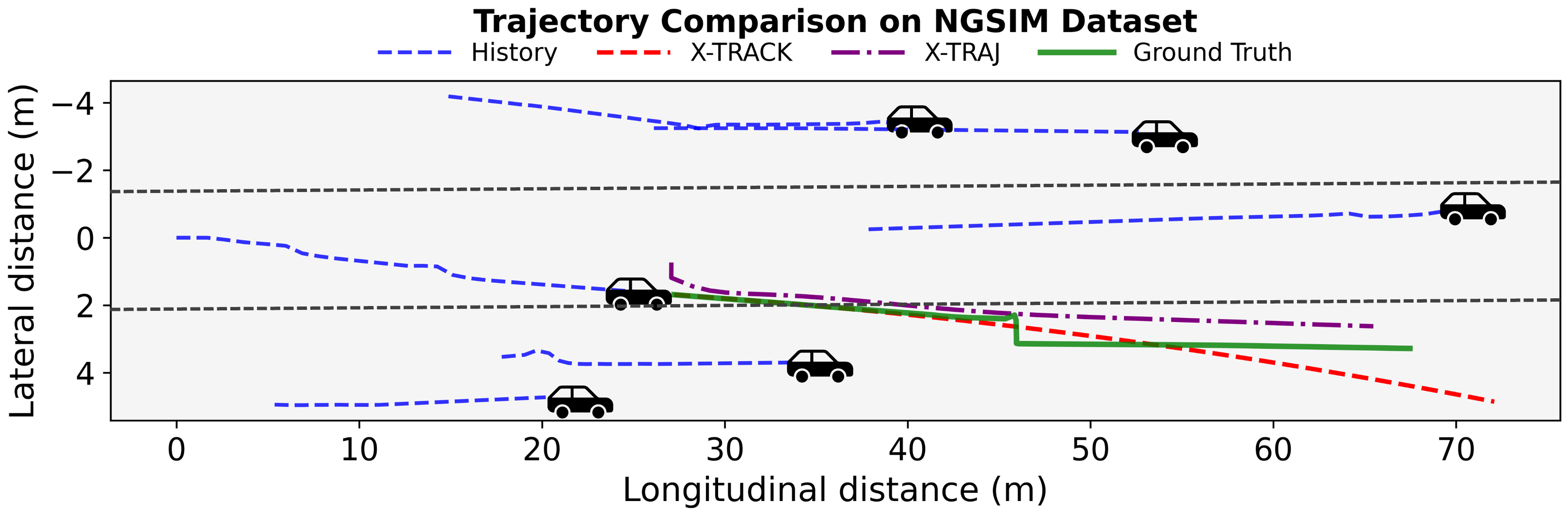
An extensive statistical analysis by Coifman et al. [28] conclusively shows that the NGSIM dataset contains significant annotation inaccuracies, giving rise to complex and physically implausible vehicle motion patterns as seen in Fig 3. In contrast, highD consists of well-annotated highway scenarios with substantially smoother and more physically consistent trajectories. Notably, Coifman et al. [28] observed that NGSIM acceleration often exhibits unrealistically large magnitudes, demonstrating that these inaccuracies disproportionately affect models that rely on acceleration either as an input or an output. As X-TRACK explicitly enforces constraints on acceleration through its kinematic layer, its performance is directly impacted by such inaccuracies.
As a result, while X-TRAJ is able to overfit these annotation artifacts and achieve lower displacement errors, X-TRACK prioritizes physically consistent motion, which may lead to higher displacement errors when evaluated against noisy or physically implausible ground truth labels. This directly explains why the kinematic layer yields significant performance improvements on highD but does not consistently translate into gains on NGSIM.
Another contributing factor to the weaker performance on NGSIM is the limited number of training samples extracted to create a balanced dataset. Since the original NGSIM data is severely imbalanced, training on the entire dataset would bias the model toward dominant keep-lane behavior. Therefore, after preprocessing, only scenarios were retained, approximately times fewer than in highD. This reduction further increases the sensitivity of physics-constrained models to annotation noise and limits the model’s ability to generalize.

(a) Keep Lane scenario

(b) Lane Change scenario
V-A Ablation Study on xLSTM Variants in X-TRACK
| Encoder | Decoder | ADE[m] | FDE[m]@5s |
|---|---|---|---|
| LSTM | sLSTM | 0.63 | 1.78 |
| sLSTM | sLSTM | 0.57 | 1.78 |
| LSTM | LSTM | 0.65 | 1.85 |
| sLSTM | LSTM | 0.56 | 1.76 |
Table III shows the ADE and FDE metrics of X-TRACK on the highD dataset, using either LSTM or sLSTM for the encoder-decoder combination. With LSTM as decoder, switching the encoder from LSTM to sLSTM gives better ADE and FDE metrics. Similarly, with sLSTM as decoder, switching the encoder from LSTM to sLSTM also produces lower errors. It was observed that an sLSTM encoder and an LSTM decoder yield the lowest error among all configurations. The worst performance is observed when LSTM is used both as an encoder and as a decoder, and all the other configurations show similar performance. The sLSTM encoder in combination with the LSTM decoder achieves and performance improvement in ADE and FDE on highD, respectively, than the conventional LSTM encoder-decoder architecture with an integrated physics-based kinematic model.
VI Conclusion
This paper introduced a novel xLSTM-based framework for highway vehicle trajectory prediction. The paper presents X-TRAJ as the first application of xLSTM to trajectory prediction, along with its physics-augmented extension X-TRACK. On highD, X-TRACK reduces the prediction error by and at -second and -second prediction, respectively, corresponding to approximately and lower error compared to the strongest baseline, GFTNNv2 [22].
In the case of highD, X-TRACK achieves an improvement of up to at a -second and about at a -second prediction horizon as compared to X-TRAJ, demonstrating that the use of non-holonomic vehicle constraints leads to smoother and physically consistent predictions. The kinematic module enables more accurate prediction of highway trajectories as the physical laws of vehicle dynamics are known and need not be inferred from the data in the case of deep learning-based models.
X-TRACK consistently outperforms state-of-the-art baselines in the case of the highD dataset. The evaluation on the NGSIM dataset indicates that X-TRACK is among the state-of-the-art models, though with the annotation inaccuracies causing non-realistic driving trajectories and the reduced dataset size in NGSIM, making it difficult for X-TRACK to predict accurate trajectories, and therefore, the results are less statistically significant as compared to the highD dataset.
These findings suggest that physics-based priors, when combined with data-driven sequence models, bridge the gap between predictive accuracy and physical consistency for highway trajectory prediction. While our current scope is limited to highway scenarios, future work will extend the framework by integrating richer contextual information, such as detailed road structure and HD map data, to improve scenario representation. Incorporating multi-modal prediction and uncertainty quantification offers a natural extension to capture multiple plausible future trajectories. Furthermore, the proposed xLSTM architecture could also be extended to urban driving datasets in order to evaluate its performance under more diverse and complex traffic environments.
Acknowledgment
This research was supported by Technische Hochschule Augsburg and the Hightech Agenda Bavaria, funded by the Free State of Bavaria, Germany. The authors would like to thank their colleagues at Data Science und Autonome Systeme Technologietransferzentrum (TTZ) Landsberg for their insightful discussions and support.
References
- [1] M. Bahari, H. Caesar, N. Navab, and T. F. C. de Campos, “Vehicle trajectory prediction works, but not everywhere,” in Proceedings of the IEEE/CVF Conference on Computer Vision and Pattern Recognition (CVPR), New Orleans, LA, USA, 2022, pp. 17 102–17 112.
- [2] S. Hochreiter and J. Schmidhuber, “Long short-term memory,” Neural Computation, vol. 9, no. 8, pp. 1735–1780, 1997.
- [3] N. Deo and M. M. Trivedi, “Convolutional social pooling for vehicle trajectory prediction,” in Proceedings of the IEEE Conference on Computer Vision and Pattern Recognition (CVPR), 2018, pp. 1549–15 498.
- [4] K. Messaoud, I. Yahiaoui, A. Verroust-Blondet, and F. Nashashibi, “Attention based vehicle trajectory prediction,” IEEE Transactions on Intelligent Vehicles, pp. 175–185, 2021.
- [5] X. Mo, Y. Xing, and C. Lv, “Graph and recurrent neural network-based vehicle trajectory prediction for highway driving,” in 2021 IEEE International Intelligent Transportation Systems Conference (ITSC). IEEE, 2021, pp. 1934–1939.
- [6] H. Cui et al., “Deep kinematic models for kinematically feasible vehicle trajectory predictions,” in Proceedings of the IEEE International Conference on Robotics and Automation (ICRA), Paris, France, 2020, pp. 10 563–10 569.
- [7] M. Beck, K. Pöppel, M. Spanring, A. Auer, O. Prudnikova, M. Kopp, G. Klambauer, J. Brandstetter, and S. Hochreiter, “xlstm: Extended long short-term memory,” Advances in Neural Information Processing Systems, vol. 37, pp. 107 547–107 603, 2024.
- [8] G. Gil, P. Duhamel-Sebline, and A. Mccarren, “An evaluation of deep learning models for stock market trend prediction,” arXiv preprint arXiv:2408.12408, 2024.
- [9] M. Alharthi and A. Mahmood, “xlstmtime: Long-term time series forecasting with xlstm,” AI, vol. 5, no. 3, pp. 1482–1495, 2024, https://www.mdpi.com/2673-2688/5/3/71. [Online]. Available: https://www.mdpi.com/2673-2688/5/3/71
- [10] M. Kraus, F. Divo, D. S. Dhami, and K. Kersting, “xLSTM-mixer: Multivariate time series forecasting by mixing via scalar memories,” in Proc. 39th Annu. Conf. Neural Information Processing Systems (NeurIPS), 2025. [Online]. Available: https://openreview.net/forum?id=JlVn0XRpy0
- [11] A. Auer, P. Podest, D. Klotz, S. Böck, G. Klambauer, and S. Hochreiter, “Tirex: Zero-shot forecasting across long and short horizons with enhanced in-context learning,” in Proc. 39th Annu. Conf. Neural Information Processing Systems (NeurIPS), 2025.
- [12] Y. Huang, J. Du, Z. Yang, Z. Zhou, L. Zhang, and H. Chen, “A survey on trajectory-prediction methods for autonomous driving,” IEEE Transactions on Intelligent Vehicles, vol. 7, no. 3, pp. 652–674, 2022.
- [13] S. Lefèvre, D. Vasquez, and C. Laugier, “A survey on motion prediction and risk assessment for intelligent vehicles,” Robomech Journal, vol. 1, 2014.
- [14] P. Veličković, G. Cucurull, A. Casanova, A. Romero, P. Liò, and Y. Bengio, “Graph attention networks,” in International Conference on Learning Representations (ICLR), 2018. [Online]. Available: https://openreview.net/forum?id=rJXMpikCZ
- [15] Z. Ding, Z. Yao, and H. Zhao, “Ra-gat: Repulsion and attraction graph attention for trajectory prediction,” in Proceedings of the IEEE International Conference on Intelligent Transportation Systems (ITSC), 2021, pp. 734–741.
- [16] Y. Wu, G. Chen, Z. Li, L. Zhang, L. Xiong, Z. Liu, and A. Knoll, “Hsta: A hierarchical spatio-temporal attention model for trajectory prediction,” IEEE Transactions on Intelligent Transportation Systems, vol. 70, pp. 11 295–11 307, 2021.
- [17] X. Chen, H. Zhang, F. Zhao, Y. Cai, H. Wang, and Q. Ye, “Vehicle trajectory prediction based on intention-aware non-autoregressive transformer with multi-attention learning for internet of vehicles,” IEEE Transactions on Instrumentation and Measurement, vol. 71, pp. 1–12, 2022.
- [18] M. Neumeier, S. Dorn, M. Botsch, and W. Utschick, “Reliable trajectory prediction and uncertainty quantification with conditioned diffusion models,” in Proceedings of the IEEE/CVF Conference on Computer Vision and Pattern Recognition (CVPR) Workshops, Jun. 2024, pp. 3461–3470.
- [19] M. Botsch and W. Utschick, Fahrzeugsicherheit und automatisiertes Fahren: Methoden der Signalverarbeitung und des maschinellen Lernens. München: Hanser, 2020.
- [20] N. M. Yusof, J. Karjanto, J. Terken, F. Delbressine, M. Z. Hassan, and M. Rauterberg, “The exploration of autonomous vehicle driving styles: Preferred longitudinal, lateral, and vertical accelerations,” in Proceedings of the 8th International Conference on Automotive User Interfaces and Interactive Vehicular Applications, 2016, pp. 245–252.
- [21] J. Kontos, B. Kránicz, and Á. Vathy-Fogarassy, “Prediction for future yaw rate values of vehicles using long short-term memory network,” Sensors, vol. 23, no. 12, 2023.
- [22] M. Neumeier, S. Dorn, M. Botsch, and W. Utschick, “Prediction and interpretation of vehicle trajectories in the graph spectral domain,” in 2023 IEEE 26th International Conference on Intelligent Transportation Systems (ITSC), 2023, pp. 1172–1179.
- [23] M. Neumeier, A. Tollkühn, M. Botsch, and W. Utschick, “A multidimensional graph fourier transformation neural network for vehicle trajectory prediction,” in Proceedings of the 2022 IEEE 25th International Conference on Intelligent Transportation Systems (ITSC), Macau, China, 2022, pp. 687–694.
- [24] A. Paszke, S. Gross, S. Chintala, G. Chanan, E. Yang, Z. DeVito, Z. Lin, A. Desmaison, L. Antiga, and T. K., “Automatic differentiation in pytorch,” in Proceedings of the NIPS Autodiff Workshop: The Future of Gradient-Based Machine Learning Software and Techniques, December 2017.
- [25] M. Fey and J. E. Lenssen, “Fast graph representation learning with PyTorch Geometric,” in ICLR Workshop on Representation Learning on Graphs and Manifolds, 2019.
- [26] D. P. Kingma and J. Ba, “Adam: A method for stochastic optimization,” in Proceedings of the 3rd International Conference on Learning Representations (ICLR), May 2015.
- [27] D. E. Benrachou, S. Glaser, M. Elhenawy, and A. Rakotonirainy, “Graph-based spatial-temporal attentive network for vehicle trajectory prediction in automated driving,” IEEE Transactions on Intelligent Transportation Systems, 2025.
- [28] B. Coifman and L. Li, “A critical evaluation of the next generation simulation (ngsim) vehicle trajectory dataset,” Transportation Research Part B: Methodological, vol. 105, pp. 362–377, 2017. [Online]. Available: https://www.sciencedirect.com/science/article/pii/S0191261517300838