Quantum separability criteria from bipartite systems to multipartite systems based on generalized Bloch representation

Linwei Li School of Mathematical and Sciences, Harbin Engineering University, Harbin 150001, China Chunlin Yang School of Mathematical and Sciences, Harbin Engineering University, Harbin 150001, China Hongmei Yao hongmeiyao@163.com School of Mathematical and Sciences, Harbin Engineering University, Harbin 150001, China Aimin Xu School of Mathematical and Sciences, Qufu Normal University, Qufu 273165, China Zhaobing Fan School of Mathematical and Sciences, Harbin Engineering University, Harbin 150001, China Shaoming Fei feishm@cnu.edu.cn School of Mathematical Sciences, Capital Normal University, Beijing 100048, China

Abstract

Quantum entanglement serves as a fundamental resource in quantum information theory. This paper presents a comprehensive framework of separability criteria for detecting bipartite and multipartite entanglements. We construct a novel parameterized extended correlation tensor via the generalized Bloch representation under an arbitrary orthogonal basis, which improves the performance of entanglement detection. Moreover, we employ the generalized matrix unfolding to generalize the extended correlation tensor construction to multipartite systems, obtaining separability criteria for multipartite entanglement. Detailed examples demonstrate that our separability criteria exhibit enhanced capability in detecting entanglement.

I Introduction

Quantum entanglement, a cornerstone of quantum information processing Nielsen and Chuang (2010); Horodecki et al. (2009a); Huo et al. (2026); Li et al. (2025a), underpins the theoretical foundations and practical applications of quantum computing DiVincenzo (1995), quantum communication Bennett et al. (1993); Xu et al. (2020); Xing et al. (2024); Li et al. (2025b), quantum cryptography Ekert (1991), and quantum simulation Lloyd (1996). Distinguishing entangled quantum states from separable ones is essential for ensuring the effectiveness and security of these quantum technologies.

Separability criteria provide crucial tools in entanglement detection. Numerous separability criteria have been proposed, including the positive map criterion Peres (1996); Horodecki et al. (1996); Li et al. (2024), computable cross-norm or realignment criteria Rudolph (2003, 2005); Chen and Wu (2002); Sun et al. (2025), as well as criteria based on covariance matrices Gühne et al. (2007) and Bloch representation de Vicente (2007). While highly effective for bipartite systems, the extension of these criteria to multipartite mixed states remains challenging, primarily due to the intricate and richer entanglement structures in such systems. To address this complexity, tensor theory Bu et al. (2015); Yao et al. (2015, 2016); Sun et al. (2016, 2018) has emerged as a powerful tool for characterizing correlations in multipartite systems. This approach captures the global properties of quantum states through correlation tensors, moving beyond local attributes and offering new perspectives for separability analysis.

Significant progress has been made in developing separability criteria based on correlation tensors. For instance, de Vicente de Vicente (2007) established an upper bound on the trace norm of the correlation tensor for separable bipartite states by using the Bloch representation. Shen et al. Shen et al. (2016) introduced parameters to an extended correlation tensor, deriving new bounds for both bipartite and multipartite states. Subsequent works have explored various bases for the Bloch representation, such as the Heisenberg–Weyl basis Chang et al. (2018); Zhao et al. (2022a), the canonical basis Sarbicki et al. (2020), and the Weyl basis Huang et al. (2022), leading to a diversity of separability criteria. More recently, Zhu et al. Zhu et al. (2023) constructed two novel matrices based on the Bloch representation to propose a separability criterion for bipartite systems. Huang et al. Huang et al. (2024) further advanced this line of research by adopting an arbitrary orthogonal basis, presenting a unified form of extended correlation tensors and a corresponding separability criterion for bipartite states. Despite these advances, existing Bloch‑representation‑based criteria vary in their tensor constructions and basis choices. A unified framework that is naturally applicable to bipartite and multipartite systems remains an interesting and challenging problem.

In this work, we propose such a framework based on a novel parameterized extended correlation tensor. By introducing independent vector parameters $\bm{u},\bm{v},\bm{\alpha},\bm{\beta}$ into the generalized Bloch representation under an arbitrary orthogonal basis, our bipartite criterion offers enhanced detection power and, with specific parameter choices, reduces to several existing ones. To extend this framework to multipartite systems, we employ the generalized matricization Bader and Kolda (2006); Kolda and Bader (2009), which flattens multiple dimensions of a tensor simultaneously into the rows or columns of the resulting matrix. While matricization has been used in multipartite separability studies, our key contribution is to combine it with the parameterized extended correlation tensor and provide criteria for detecting multipartite entanglement and genuine multipartite entanglement.

The paper is structured as follows. Sect. II introduces some notations and definitions. Sect. III details the construction of the novel parameterized extended correlation tensor for bipartite states and presents the corresponding separability criterion, followed by two examples for detecting entanglement. Sect. IV generalizes the parameterized extended correlation tensor to $N$ -partite systems using the generalized matricization. Biseparability and full separability criteria are provided and demonstrated with examples. Sect. V discusses the conclusion and outlook.

II Preliminaries

Let us begin by recalling some notations and definitions. For integers $M,N$ with $M\leq N$ , we denote $[M,N]=\left\{M,M+1,\cdots,N\right\}$ , $[N]=\left\{1,\cdots,N\right\}$ for $N\geq 1$ , and $[0]=\emptyset$ .

Denote $\bm{e}_{i}\in\mathbb{R}^{d}$ as the $i$ -th standard unit vector of size $d$ . Let $\mathbf{I}_{N}$ denote the $N\times N$ identity matrix. For matrices $\mathbf{A},\mathbf{B}\in\mathbb{C}^{M\times N}$ , their Hilbert-Schmidt inner product is defined as $\langle\mathbf{A},\mathbf{B}\rangle={\rm Tr}\left(\mathbf{A}^{\dagger}\mathbf{B}\right)$ ; the trace norm of $\mathbf{A}$ is defined as $\left\|\mathbf{A}\right\|_{\rm tr}={\rm Tr}\left(\sqrt{\mathbf{A}^{\dagger}\mathbf{A}}\right)$ , where ${\rm Tr}\left(\mathbf{A}\right)$ is the trace of $\mathbf{A}$ and $\mathbf{A}^{\dagger}$ is the transpose conjugate of $\mathbf{A}$ .

A tensor is a multi-dimensional array. For tensors $\mathcal{A}=\left(a_{i_{1}\cdots i_{N}}\right)\in\mathbb{C}^{d_{1}\times\cdots\times d_{N}}$ , $\mathcal{B}=\left(b_{j_{1}\cdots j_{M}}\right)\in\mathbb{C}^{d_{1}^{\prime}\times\cdots\times d_{M}^{\prime}}$ , and a matrix $\mathbf{U}=\left(u_{i_{k}^{\prime}i_{k}}\right)\in\mathbb{C}^{d_{k}^{\prime}\times d_{k}}$ , where $M\leq N$ and $k\in[N]$ , the Frobenius norm of $\mathcal{A}$ is defined as $\left\|\mathcal{A}\right\|_{F}=\sqrt{\sum_{i_{1},\cdots,i_{N}=1}^{d_{1},\cdots,d_{N}}\left|a_{i_{1}\cdots i_{N}}\right|^{2}}$ ; the tensor product of $\mathcal{A},\mathcal{B}$ is defined as $\mathcal{A}\otimes\mathcal{B}=\left(c_{k_{1}\cdots k_{N}}\right)$ with size $(d_{1}d_{1}^{\prime})\times\cdots\times(d_{M}d_{M}^{\prime})\times d_{M+1}\times\cdots\times d_{N}$ , where $c_{k_{1}\cdots k_{N}}=a_{i_{1}\cdots i_{N}}b_{j_{1}\cdots j_{M}}$ and

k_{l}=\begin{cases}(i_{l}-1)d_{l}+j_{l},&\mbox{if }l\in[M],\\ i_{l},&\mbox{if }l\in[M+1,N];\end{cases}

the outer product of $\mathcal{A},\mathcal{B}$ is defined as $\mathcal{A}\circ\mathcal{B}=\mathcal{C}=\left(c_{i_{1}\cdots i_{N}j_{1}\cdots j_{M}}\right)$ with size $d_{1}\times\cdots\times d_{N}\times d_{1}^{\prime}\times\cdots\times d_{M}^{\prime}$ , where $c_{i_{1}\cdots i_{N}j_{1}\cdots j_{M}}=a_{i_{1}\cdots i_{N}}b_{j_{1}\cdots j_{M}}$ ; the $k$ -mode product of $\mathcal{A}$ and $\mathbf{U}$ is denoted as $\mathcal{A}\times_{k}\mathbf{U}$ with size $d_{1}\times\cdots\times d_{k-1}\times d_{k}^{\prime}\times d_{k+1}\times\cdots\times d_{N}$ , whose entries are given by $\left(\mathcal{A}\times_{k}\mathbf{U}\right)_{i_{1}\cdots i_{k-1}i_{k}^{\prime}i_{k+1}\cdots i_{N}}=\sum_{i_{k}=1}^{d_{k}}a_{i_{1}\cdots i_{k-1}i_{k}i_{k+1}\cdots i_{N}}u_{i_{k}^{\prime}i_{k}}$ .

For $k\in[N]$ , the $k$ -mode matrix unfolding De Lathauwer et al. (2000) of a tensor $\mathcal{A}=\sum_{i_{1},\cdots,i_{N}=1}^{d_{1},\cdots,d_{N}}a_{i_{1}\cdots i_{N}}\bm{e}_{i_{1}}^{(1)}\circ\cdots\circ\bm{e}_{i_{N}}^{(N)}$ is a matrix $\mathbf{A}_{(k)}$ of size $d_{k}\times\left(\prod_{j\in[N]\setminus\{k\}}d_{j}\right)$ , defined by

\displaystyle\mathbf{A}_{(k)}=\sum_{i_{1},\cdots,i_{N}=1}^{d_{1},\cdots,d_{N}}a_{i_{1}\cdots i_{N}}\bm{e}_{i_{1}}^{(1)}\left(\left(\bigotimes_{j=k+1}^{N}\bm{e}_{i_{j}}^{(j)}\right)\otimes\left(\bigotimes_{j=1}^{k-1}\bm{e}_{i_{j}}^{(j)}\right)\right)^{\rm T}.

The $k$ -mode matrix unfolding of tensors maps only one dimension to the rows of the resulting matrix and the others to the columns. Naturally, one can map multiple dimensions to the rows, leading to the generalized matricization Bader and Kolda (2006); Kolda and Bader (2009). Let $R=\left\{r_{1},\cdots,r_{k}\right\}$ and $C=\left\{c_{1},\cdots,c_{N-k}\right\}$ be two disjoint ascending ordered sets referred to as the rows and the columns, where $R\cup C=[N]$ and $k\in[0,N]$ . The unfolding is performed in backward cyclic order with two specified modes, similar to Ref. De Lathauwer et al. (2000). For $n\in[k]$ and $m\in[N-k]$ , we refer to the ${(R,n;C,m)}$ -mode matrix unfolding of $\mathcal{A}$ as the generalized matricization, which gives a matrix of size $\left(\prod_{i\in R}d_{i}\right)\times\left(\prod_{i\in C}d_{i}\right)$ , defined by

	$\displaystyle\mathbf{A}_{(R,n;C,m)}=$	$\displaystyle\sum_{i_{1},\cdots,i_{N}=1}^{d_{1},\cdots,d_{N}}a_{i_{1}\cdots i_{N}}\left(\left(\bigotimes_{j=n+1}^{k}\bm{e}_{i_{r_{j}}}^{(r_{j})}\right)\otimes\left(\bigotimes_{j=1}^{n}\bm{e}_{i_{r_{j}}}^{(r_{j})}\right)\right)$
		$\displaystyle\cdot\left(\left(\bigotimes_{j=m+1}^{N-k}\bm{e}_{i_{c_{j}}}^{(c_{j})}\right)\otimes\left(\bigotimes_{j=1}^{m}\bm{e}_{i_{c_{j}}}^{(c_{j})}\right)\right)^{\rm T}.$

For a tensor $\mathcal{A}\in\mathbb{C}^{d_{1}\times\cdots\times d_{N}}$ , its trace norm can be defined as $\left\|\mathcal{A}\right\|_{\rm tr}=\max_{\begin{subarray}{c}R\cup C=[N],R\cap C=\emptyset\\ \left|R\right|=k>0,\left|C\right|=N-k>0\\ n\in[k],m\in[N-k]\end{subarray}}\left\{\left\|\mathbf{A}_{(R,n;C,m)}\right\|_{\rm tr}\right\}$ .

The vectorization of a matrix $\mathbf{A}=\left(a_{ij}\right)$ is a vector ${\rm vec}\left(\mathbf{A}\right)=\left(a_{11},\cdots,a_{M1},a_{12},\cdots,a_{M2},\cdots\!,a_{1N},\cdots,a_{MN}\right)^{\rm T}$ , where the element $a_{ij}$ is at the position with the row index $\left(j-1\right)M+i$ . The $k$ -mode vectorization of a tensor $\mathcal{A}$ is defined by ${\rm vec}_{k}\left(\mathcal{A}\right)={\rm vec}\left(\mathbf{A}_{(k)}\right)$ . Especially, for a vector $\bm{v}$ and a matrix $\mathbf{A}$ , it holds that ${\rm vec}_{1}\left(\bm{v}\right)=\bm{v}$ , ${\rm vec}_{1}\left(\mathbf{A}\right)={\rm vec}\left(\mathbf{A}\right)$ , and ${\rm vec}_{2}\left(\mathbf{A}\right)={\rm vec}\left(\mathbf{A}^{\rm T}\right)$ .

III Separability criterion for bipartite systems

In this section, based on the generalized Bloch representation, we present a novel construction of the extended correlation tensor for bipartite quantum states, and derive the corresponding separability criterion. Two examples are provided to demonstrate the enhanced entanglement detection ability of the criterion. Moreover, we explore the relations between our criterion and the existing ones.

III.1 Separability criterion

Consider a $d$ -dimensional Hilbert space $\mathcal{H}_{d}$ . Let $\mathcal{L}\left(\mathcal{H}_{d}\right)$ be the space of linear operators acting on $\mathcal{H}_{d}$ and $\left\{\mathbf{G}_{i}\right\}_{i=0}^{d^{2}-1}$ be an orthogonal basis in $\mathcal{L}\left(\mathcal{H}_{d}\right)$ satisfying $\mathbf{G}_{0}=\mathbf{I}_{d}$ , $\langle\mathbf{G}_{i},\mathbf{G}_{j}\rangle=\kappa\delta_{ij}$ and ${\rm Tr}(\mathbf{G}_{i})=0$ , where $\delta_{ij}$ is the Kronecker delta function, $\kappa\geq 1$ is the normalized constant of the basis, $i,j\in[d^{2}-1]$ . The value of $\kappa$ depends on the detailed choice of orthogonal basis, for example, $\kappa=2$ ( $\kappa=d$ ) if the orthogonal basis is chosen to be the Pauli operators (Weyl operators or Heisenberg-Weyl operators).

A quantum state $\rho\in\mathcal{H}_{d}$ can be expanded in the basis $\left\{\mathbf{G}_{i}\right\}_{i=0}^{d^{2}-1}$ , yielding the following generalized Bloch representation,

\rho=\frac{1}{d}\left(\mathbf{I}_{d}+\sum_{i=1}^{d^{2}-1}t_{i}\mathbf{G}_{i}\right),

(1)

where the coefficient $t_{i}=\frac{d}{\kappa}{\rm Tr}\left(\rho\mathbf{G}_{i}\right)$ . $\mathcal{T}=\left(t_{i}\right)\in\mathbb{C}^{d^{2}-1}$ is the correlation tensor (or generalized Bloch vector) of $\rho$ . Ref. Huang et al. (2024) upper bounded the Frobenius norm of $\mathcal{T}$ .

Lemma 1.

Huang et al. (2024) For any quantum state $\rho\in\mathcal{H}_{d}$ , its correlation tensor $\mathcal{T}$ satisfies $\left\|\mathcal{T}\right\|_{F}^{2}\leq\frac{d^{2}-d}{\kappa}$ .

Consider a bipartite quantum system $\mathcal{H}_{d_{A}}\otimes\mathcal{H}_{d_{B}}$ with dimensions $d_{A}$ and $d_{B}$ of subsystems , respectively. Choose arbitrary orthogonal bases

\left\{\mathbf{G}_{i}^{(A)}\right\}_{i=0}^{d_{A}^{2}-1},\quad\left\{\mathbf{G}_{j}^{(B)}\right\}_{j=0}^{d_{B}^{2}-1},

(2)

in the operator spaces $\mathcal{L}(\mathcal{H}_{d_{A}})$ and $\mathcal{L}(\mathcal{H}_{d_{B}})$ , respectively, satisfying

\begin{gathered}\mathbf{G}^{(A)}_{0}=\mathbf{I}^{(A)}_{d_{A}},\langle\mathbf{G}_{i}^{(A)},\mathbf{G}_{i^{\prime}}^{(A)}\rangle=\kappa_{A}\delta_{ii^{\prime}},{\rm Tr}\left(\mathbf{G}_{i}^{(A)}\right)=0,\\ \mathbf{G}^{(B)}_{0}=\mathbf{I}^{(B)}_{d_{B}},\langle\mathbf{G}_{j}^{(B)},\mathbf{G}_{j^{\prime}}^{(B)}\rangle=\kappa_{B}\delta_{jj^{\prime}},{\rm Tr}\left(\mathbf{G}_{j}^{(B)}\right)=0,\end{gathered}

(3)

where $\kappa_{A},\kappa_{B}\geq 1$ , $i,i^{\prime}\in[d_{A}^{2}-1]$ , $j,j^{\prime}\in[d_{B}^{2}-1]$ . Any bipartite state $\rho^{(AB)}\in\mathcal{H}_{d_{A}}\otimes\mathcal{H}_{d_{B}}$ can be expanded in the orthogonal bases specified by Eq. (2), yielding the following generalized Bloch representation,

$\displaystyle\rho^{(AB)}=$	$\displaystyle\frac{1}{d_{A}d_{B}}\left(\mathbf{I}_{d_{A}}^{(A)}\otimes\mathbf{I}_{d_{B}}^{(B)}\right.$	(4)
	$\displaystyle+\sum_{i=1}^{d_{A}^{2}-1}t_{i}^{(A)}\mathbf{G}_{i}^{(A)}\otimes\mathbf{I}_{d_{B}}^{(B)}+\sum_{j=1}^{d_{B}^{2}-1}t_{j}^{(B)}\mathbf{I}_{d_{A}}^{(A)}\otimes\mathbf{G}_{j}^{(B)}$
	$\displaystyle\left.+\sum_{i=1}^{d_{A}^{2}-1}\sum_{j=1}^{d_{B}^{2}-1}t_{ij}^{(AB)}\mathbf{G}_{i}^{(A)}\otimes\mathbf{G}_{j}^{(B)}\right),$

where the coefficients are given by

\begin{gathered}t_{i}^{(A)}=\frac{d_{A}}{\kappa_{A}}\mathrm{Tr}\left(\rho^{(AB)}\left(\mathbf{G}_{i}^{(A)}\otimes\mathbf{I}_{d_{B}}^{(B)}\right)\right),\\ t_{j}^{(B)}=\frac{d_{B}}{\kappa_{B}}\mathrm{Tr}\left(\rho^{(AB)}\left(\mathbf{I}_{d_{A}}^{(A)}\otimes\mathbf{G}_{j}^{(B)}\right)\right),\\ t_{ij}^{(AB)}=\frac{d_{A}d_{B}}{\kappa_{A}\kappa_{B}}\mathrm{Tr}\left(\rho^{(AB)}\left(\mathbf{G}_{i}^{(A)}\otimes\mathbf{G}_{j}^{(B)}\right)\right).\end{gathered}

$\mathcal{T}^{(A)}=\left(t_{i}^{(A)}\right)\in\mathbb{C}^{d_{A}^{2}-1}$ , $\mathcal{T}^{(B)}=\left(t_{j}^{(B)}\right)\in\mathbb{C}^{d_{B}^{2}-1}$ , and $\mathcal{T}^{(AB)}=(t_{ij}^{(AB)})\in\mathbb{C}^{(d_{A}^{2}-1)\times(d_{B}^{2}-1)}$ are the correlation tensors of $\rho^{(AB)}$ for the corresponding (sub)systems.

Given a quantum state $\rho^{(AB)}\in\mathcal{H}_{d_{A}}\otimes\mathcal{H}_{d_{B}}$ , we construct the extended correlation tensor based on the correlation tensor and the reduced density matrices. For any vectors $\bm{u}=\left(u_{1},\cdots,u_{p_{1}}\right)^{\rm T}\in\mathbb{R}^{p_{1}}$ , $\bm{v}=\left(v_{1},\cdots,v_{p_{2}}\right)^{\rm T}\in\mathbb{R}^{P_{2}}$ , $\bm{\alpha}=\left(a_{1},\cdots,a_{q_{1}}\right)^{\rm T}\in\mathbb{R}^{q_{1}}$ , and $\bm{\beta}=\left(b_{1},\cdots,b_{q_{2}}\right)^{\rm T}\in\mathbb{R}^{q_{2}}$ , the extended correlation tensor has a size of $\left(p_{1}+q_{1}\left(d_{A}^{2}-1\right)\right)\times\left(p_{2}+q_{2}\left(d_{B}^{2}-1\right)\right)$ and is defined by

\mathcal{M}_{\bm{u},\bm{v},\bm{\alpha},\bm{\beta}}^{(A|B)}(\rho^{(AB)})=\begin{pmatrix}\bm{u}\bm{v}^{\rm T}&\bm{u}\left(\bm{\beta}\otimes\mathcal{T}^{(B)}\right)^{\rm T}\\ \left(\bm{\alpha}\otimes\mathcal{T}^{(A)}\right)\bm{v}^{\rm T}&\bm{\alpha}\bm{\beta}^{\rm T}\otimes\mathcal{T}^{(AB)}\\ \end{pmatrix}.

(5)

A separable state $\rho^{(AB)}$ can be expressed as a convex combination of product states, $\rho^{(AB)}=\sum_{i}p_{i}\rho^{(A)}_{i}\otimes\rho^{(B)}_{i}$ , where $0\leq p_{i}\leq 1$ , $\sum_{i}p_{i}=1$ , $\rho^{(A)}_{i}$ and $\rho^{(B)}_{i}$ are pure states in $\mathcal{H}_{d_{A}}$ and $\mathcal{H}_{d_{B}}$ , respectively. Based on the extended correlation tensor, we present the main theorem of bipartite separability criterion, see proof in Appendix C.1.

Theorem 1.

If a quantum state $\rho^{(AB)}\in\mathcal{H}_{d_{A}}\otimes\mathcal{H}_{d_{B}}$ is separable, then its extended correlation tensor given by Eq. (5) satisfies

		$\displaystyle\left\\|\mathcal{M}_{\bm{u},\bm{v},\bm{\alpha},\bm{\beta}}^{(A\|B)}(\rho^{(AB)})\right\\|_{\rm tr}$		(6)
	$\displaystyle\leq$	$\displaystyle\sqrt{\left(\left\\|\bm{u}\right\\|_{F}^{2}+\left\\|\bm{\alpha}\right\\|_{F}^{2}\frac{{d_{A}}^{2}-d_{A}}{\kappa_{A}}\right)\left(\left\\|\bm{v}\right\\|_{F}^{2}+\left\\|\bm{\beta}\right\\|_{F}^{2}\frac{{d_{B}}^{2}-d_{B}}{\kappa_{B}}\right)}.$		(6)

Using the bipartite separability criterion given in Theorem 1, we detect the entanglement of two bipartite quantum states in the following examples.

Example 1.

Consider the $3\times 3$ PPT entangled state Bennett et al. (1999),

\rho=\frac{1}{4}\left(\mathbf{I}_{9}-\sum_{i=0}^{4}\ket{\varphi_{i}}\bra{\varphi_{i}}\right),

where $\ket{\varphi_{0}}=\frac{1}{\sqrt{2}}\ket{0}\left(\ket{0}-\ket{1}\right)$ , $\ket{\varphi_{1}}=\frac{1}{\sqrt{2}}\left(\ket{0}-\ket{1}\right)\ket{2}$ , $\ket{\varphi_{2}}=\frac{1}{\sqrt{2}}\ket{2}\left(\ket{1}-\ket{2}\right)$ , $\ket{\varphi_{3}}=\frac{1}{\sqrt{2}}\left(\ket{1}-\ket{2}\right)\ket{0}$ , and $\ket{\varphi_{4}}=\frac{1}{3}\left(\ket{0}+\ket{1}+\ket{2}\right)\left(\ket{0}+\ket{1}+\ket{2}\right)$ . We mix $\rho$ with white noise and consider the following state,

\rho_{p}=\frac{1-p}{9}\mathbf{I}_{9}+p\rho,

(7)

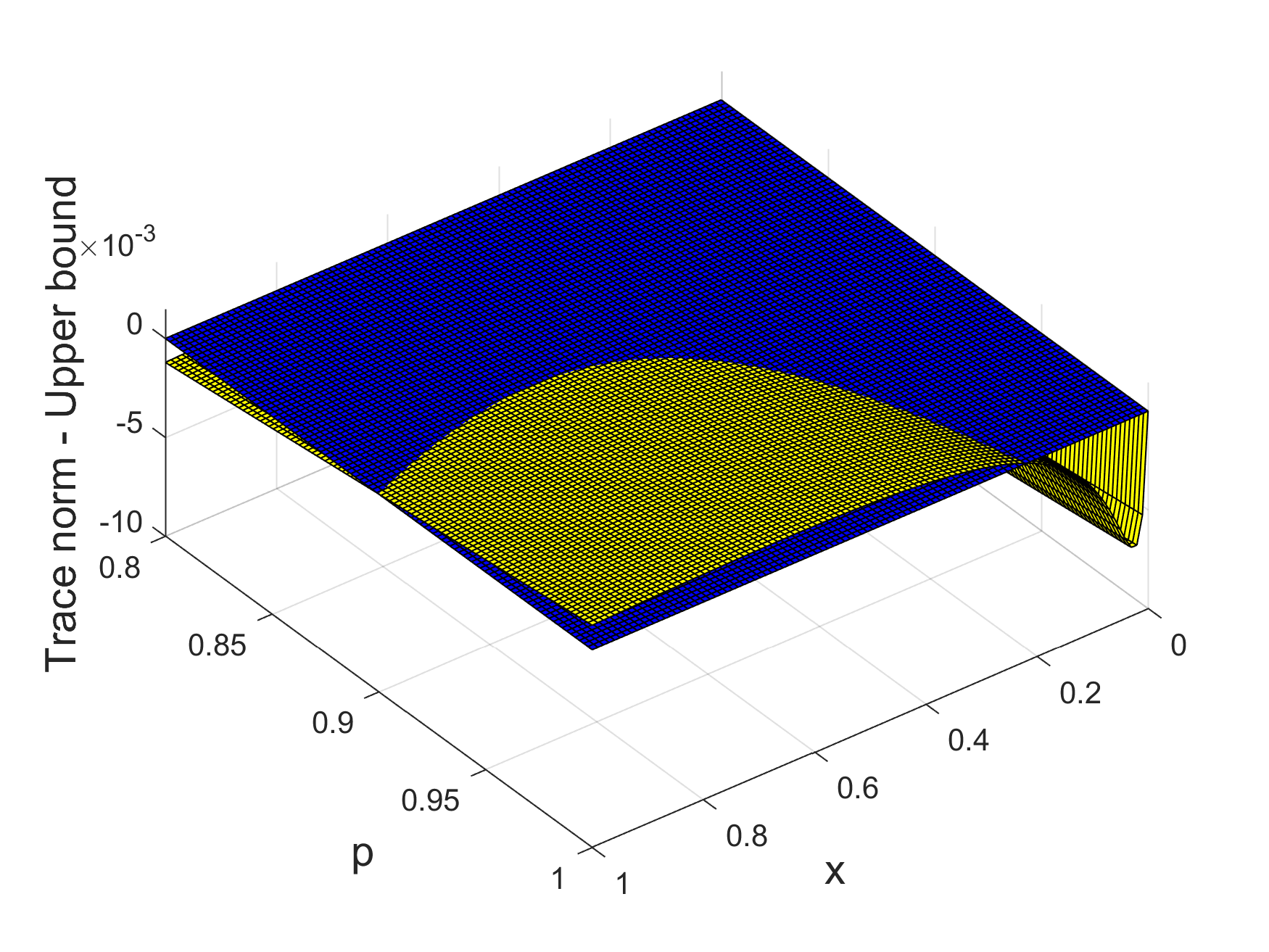
where $0\leq p\leq 1$ . in Choose the Heisenberg-Weyl operators as orthogonal bases of the bipartite system $\mathcal{H}_{d_{A}}\otimes\mathcal{H}_{d_{B}}$ , with $\kappa_{A}=d_{A}=\kappa_{B}=d_{B}=3$ . Taking $\bm{u}=\left(x,x,x,x\right)^{\rm T}$ , $\bm{v}=\left(\sqrt{x},\sqrt{x},\sqrt{x},\sqrt{x}\right)^{\rm T}$ , $\bm{\alpha}=0.063782$ and $\bm{\beta}=0.0786454$ , by Theorem 1 we detect that $\rho_{p}$ is entangled for $0.882252\leq p\leq 1$ . The result is shown in Figure 1, where the blue plane surface represents the zero plane, and the yellow curved surface represents the difference between the trace norm and the upper bound on the left and right hand sides of Eq. (6). Existing separability criteria such as CCNR Rudolph (2005), Li’s criterion Li et al. (2014), dV’s criterion de Vicente (2007), and Huang’s criterion Huang et al. (2024) can also detect the entanglement of the state $\rho_{p}$ .

Refer to caption — Figure 1: The relation between the entanglement $\rho_{p}$ and the parameters $p,x$ in Example 1, with $\bm{u}=\left(x,x,x,x\right)^{\rm T}$ , $\bm{v}=\left(\sqrt{x},\sqrt{x},\sqrt{x},\sqrt{x}\right)^{\rm T}$ , $\bm{\alpha}=0.063782$ and $\bm{\beta}=0.0786454$ .

Table 1 shows the comparison between their detection thresholds and ours. It is observed that our Theorem 1 detects the entanglement of the state $\rho_{p}$ in Eq. (7) better.

Table 1: The comparison of detection thresholds for various separability criteria for the state

\rho_{p}

in Eq. (7).

Separability criteria	Range (entanglement) of $p$
Theorem 1	$0.882252\leq p\leq 1$
Huang’s criterion Huang et al. (2024)	$0.8843<p\leq 1$
Li’s criterion Li et al. (2014)	$0.8925<p\leq 1$
CCNR Rudolph (2005)	$0.8897<p\leq 1$
dV’s criterion de Vicente (2007)	$0.9493<p\leq 1$

Example 2.

We consider the state

\rho_{p}=p\ket{\xi}\bra{\xi}+(1-p)\rho_{a},

(8)

where $0\leq p\leq 1$ ,

\rho_{a}=\frac{1}{7a+1}\begin{pmatrix}a&0&0&0&0&a&0&0\\ 0&a&0&0&0&0&a&0\\ 0&0&a&0&0&0&0&a\\ 0&0&0&a&0&0&0&0\\ 0&0&0&0&\frac{1+a}{2}&0&0&\frac{\sqrt{1-a^{2}}}{2}\\ a&0&0&0&0&a&0&0\\ 0&a&0&0&0&0&a&0\\ 0&0&a&0&\frac{\sqrt{1-a^{2}}}{2}&0&0&\frac{1+a}{2}\end{pmatrix}

is the $2\times 4$ bounded entangled state Horodecki (1997) and $\ket{\xi}=\frac{1}{\sqrt{2}}\left(\ket{00}+\ket{11}\right)$ , $0<a<1$ .

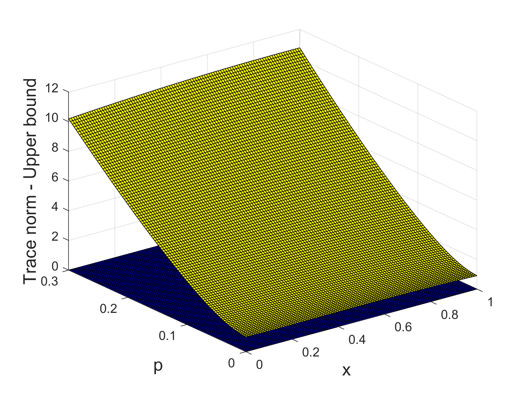
Choose the Pauli operators as the orthogonal bases of the system. So we have $\kappa_{A}=\kappa_{B}=2$ . Set $a=0.9$ , $\bm{u}=\left(x,x\right)^{\rm T}$ , $\bm{v}=\left(\sqrt{x},\sqrt{x}\right)^{\rm T}$ , $\bm{\alpha}=\left(-3.23405,1.35293\right)^{\rm T}$ and $\bm{\beta}=\left(-1.83346,-0.969888\right)^{\rm T}$ . By Theorem 1, the state $\rho_{p}$ is entangled for all $0\leq p\leq 1$ . The result is shown in Figure 2, where the blue plane surface represents zero plane, and the yellow curved surface represents the difference between the trace norm and the upper bound on the left and right hand sides of Eq. (6). Compared with the existing separability criteria, our Theorem 1 clearly detects better the entanglement of the state $\rho_{p}$ in Eq. (8), see Table 2.

Table 2: The comparison of detection thresholds for various separability criteria for the state

\rho_{p}

in Eq. (8) with

a=0.9

Separability criteria	Range (entanglement) of $p$
Theorem 1	$0\leq p\leq 1$
Sun’s criterion Sun et al. (2025)	$0.233889<p\leq 1$
Shen’s criterion Shen et al. (2016)	$0.2235<p\leq 1$
dV’s criterion de Vicente (2007)	$0.2293<p\leq 1$
Li’s criterion Li et al. (2014)	$0.2841<p\leq 1$

III.2 Relations to other separability criteria

The separability criterion for bipartite quantum systems proposed in this paper introduces parameters $\bm{u}=\left(u_{1},\cdots,u_{p_{1}}\right)^{\rm T}\in\mathbb{R}^{p_{1}}$ , $\bm{v}=\left(v_{1},\cdots,v_{p_{2}}\right)^{\rm T}\in\mathbb{R}^{p_{2}}$ , $\bm{\alpha}=\left(a_{1},\cdots,a_{q_{1}}\right)^{\rm T}\in\mathbb{R}^{q_{1}}$ and $\bm{\beta}=\left(b_{1},\cdots,b_{q_{2}}\right)^{\rm T}\in\mathbb{R}^{q_{2}}$ , where $p_{1},p_{2},q_{1},q_{2}$ are positive integers. It selects orthogonal bases $\left\{\mathbf{G}_{i}^{(A)}\right\}_{i=0}^{d_{A}^{2}-1}$ and $\left\{\mathbf{G}_{i}^{(B)}\right\}_{i=0}^{d_{B}^{2}-1}$ in the operator spaces $\mathcal{L}(\mathcal{H}_{d_{A}})$ and $\mathcal{L}(\mathcal{H}_{d_{B}})$ , respectively, satisfying Eq. (3) with $\kappa_{A},\kappa_{B}\geq 1$ . The inclusion of these parameters and the freedom in choosing orthogonal bases establish close connections between the separability criterion presented in this paper and several existing ones, while also improve the ability of entanglement detection.

In 2007, de Vicente de Vicente (2007) provided an upper bound for the trace norm of the correlation tensor $\mathcal{T}^{(AB)}$ for separable states,

\left\|\mathcal{T}^{(AB)}\right\|_{\rm tr}\leq\sqrt{\frac{{d_{A}d_{B}}\left(d_{A}-1\right)\left(d_{B}-1\right)}{4}},

where the orthogonal bases are chosen as the Pauli operators, that is, $\kappa_{A}=\kappa_{B}=2$ . Taking $\bm{u}=\bm{v}=0$ , $\bm{\alpha}=\bm{\beta}=1$ in Eq. (5), we obtain

	$\displaystyle\left\\|\mathcal{T}^{(AB)}\right\\|_{\rm tr}=$	$\displaystyle\left\\|\mathcal{M}_{0,0,1,1}^{(A\|B)}\left(\rho^{(AB)}\right)\right\\|_{\rm tr}$
	$\displaystyle\leq$	$\displaystyle\sqrt{\left(\frac{d^{2}_{A}-d_{A}}{2}\right)\left(\frac{d^{2}_{B}-d_{B}}{2}\right)}$
	$\displaystyle=$	$\displaystyle\sqrt{\frac{d_{A}d_{B}\left(d_{A}-1\right)\left(d_{B}-1\right)}{4}}.$

which implies that the conclusion in Theorem 1 reduces to that given in Ref. de Vicente (2007) with particularly fixed parameters.

In 2016, Shen et al. Shen et al. (2016) introduced parameters $x,y\in\mathbb{R}$ and the matrix $\mathbf{E}_{l\times l}$ of size $l\times l$ with all entries being one and constructed the following extended correlation tensor,

\mathcal{S}_{x,y}^{l}(\rho^{(AB)})=\begin{pmatrix}xy\mathbf{E}_{l\times l}&x\omega_{l}^{\rm T}\left(\mathcal{T}^{(B)}\right)\\ y\omega_{l}\left(\mathcal{T}^{(A)}\right)&\mathcal{T}^{(AB)}\\ \end{pmatrix},

(9)

where $\omega_{l}\left(\bm{v}\right)=\underbrace{\left(\bm{v},\cdots,\bm{v}\right)}_{l}$ and the orthogonal bases are chosen as the Pauli operators. It has been proven that for the separable quantum state $\rho^{(AB)}$ ,

\displaystyle\left\|\mathcal{S}_{x,y}^{l}(\rho^{(AB)})\right\|_{\rm tr}

\displaystyle\leq\frac{1}{2}\sqrt{\left(2lx^{2}+d^{2}_{A}-d_{A}\right)\left(2ly^{2}+d^{2}_{B}-d_{B}\right)}.

Using the extended correlation tensor given in Eq. (5) and taking $\bm{u}=\left(x,\cdots,x\right)^{\rm T}\in\mathbb{R}^{l}$ , $\bm{v}=\left(y,\cdots,y\right)^{\rm T}\in\mathbb{R}^{l}$ , $\bm{\alpha}=\bm{\beta}=1$ , we have

		$\displaystyle\left\\|\mathcal{S}_{x,y}^{l}(\rho^{(AB)})\right\\|_{\rm tr}=\left\\|\mathcal{M}_{\bm{u},\bm{v},1,1}^{(A\|B)}(\rho^{(AB)})\right\\|_{\rm tr}$
	$\displaystyle\leq$	$\displaystyle\sqrt{\left(lx^{2}+\frac{d^{2}_{A}-d_{A}}{2}\right)\left(ly^{2}+\frac{d^{2}_{B}-d_{B}}{2}\right)}$
	$\displaystyle=$	$\displaystyle\frac{1}{2}\sqrt{\left(2lx^{2}+d^{2}_{A}-d_{A}\right)\left(2ly^{2}+d^{2}_{B}-d_{B}\right)}.$

It can be seen that our separability criterion covers the one given in Ref. Shen et al. (2016). In addition, if we take $\kappa_{A},\kappa_{B}>2$ , then the trace norm of our extended correlation tensor in Eq. (5) has a lower upper bound.

In 2018, Chang et al. Chang et al. (2018) constructed the extended correlation tensor that is structurally identical to Eq. (9), but adopted the Heisenberg-Weyl operators as orthogonal bases, resulting in $\kappa_{A}=d_{A}$ and $\kappa_{B}=d_{B}$ . Then they provided the following separable criterion,

\left\|\mathcal{S}_{x,y}^{l}(\rho^{(AB)})\right\|_{\rm tr}\leq\sqrt{\left(lx^{2}+d_{A}-1\right)\left(ly^{2}+d_{B}-1\right)},

which is also a special case of our separability criterion with $\bm{u}=\left(x,\cdots,x\right)^{\rm T}\in\mathbb{R}^{l}$ , $\bm{v}=\left(y,\cdots,y\right)^{\rm T}\in\mathbb{R}^{l}$ and $\bm{\alpha}=\bm{\beta}=1$ .

In 2020, Sarbicki et al. Sarbicki et al. (2020) employed the canonical basis to establish a generalized Bloch representation for bipartite quantum states, where the canonical bases $\left\{\mathbf{G}_{i}^{(A)}\right\}_{i=0}^{d_{A}^{2}-1}$ and $\left\{\mathbf{G}_{i}^{(B)}\right\}_{i=0}^{d_{B}^{2}-1}$ are orthogonal and satisfy $\langle\mathbf{G}_{i}^{(A)},\mathbf{G}_{j}^{(A)}\rangle=\delta_{ij}$ , $\langle\mathbf{G}_{i}^{(B)},\mathbf{G}_{j}^{(B)}\rangle=\delta_{ij}$ . The resulting coefficients of generalized Bloch representation form a matrix $\mathbf{C}^{\rm can}\in\mathbb{C}^{d^{2}_{A}\times d^{2}_{B}}$ , from which they derived the following separability criterion,

\left\|\mathbf{D}^{A}_{x}\mathbf{C}^{\rm can}\mathbf{D}^{B}_{y}\right\|_{\rm tr}\leq\sqrt{\left(\frac{d_{A}-1+x^{2}}{d_{A}}\right)\left(\frac{d_{B}-1+y^{2}}{d_{B}}\right)},

where $\mathbf{D}^{A}_{x}={\rm diag}\left\{x,1,\dots,1\right\}\in\mathbb{R}^{d^{2}_{A}\times d^{2}_{A}}$ and $\mathbf{D}^{B}_{y}={\rm diag}\left\{y,1,\dots,1\right\}\in\mathbb{R}^{d^{2}_{B}\times d^{2}_{B}}$ , $x,y\geq 0$ . In fact, the matrix $\mathbf{D}^{A}_{x}\mathbf{C}^{\rm can}\mathbf{D}^{B}_{y}$ is equivalent to a special case of the extended correlation tensor proposed in this work. Taking $\bm{u}=\frac{x}{\sqrt{d_{A}}}$ , $\bm{v}=\frac{y}{\sqrt{d_{B}}}$ , $\bm{\alpha}=\bm{\beta}=1$ , $\kappa_{A}=\kappa_{B}=1$ in Eq. (5), we obtain

		$\displaystyle\left\\|\mathcal{M}_{\bm{u},\bm{v},1,1}^{(A\|B)}\left(\rho^{(AB)}\right)\right\\|_{\rm tr}$
	$\displaystyle\leq$	$\displaystyle\sqrt{\left(\frac{d^{2}_{A}\left(d_{A}-1\right)+x^{2}}{d_{A}}\right)\left(\frac{d^{2}_{B}\left(d_{B}-1\right)+y^{2}}{d_{B}}\right)},$

where the upper bound differs from the one in Ref. Sarbicki et al. (2020) by additional factors $d_{A}^{2}$ and $d_{B}^{2}$ , because the generalized Bloch representations in Ref. Sarbicki et al. (2020) and this paper differ by a scale $\frac{1}{d_{A}d_{B}}$ so that the upper bounds of the correlation tensor for a monomer quantum state used in the proof differ by a scale $d^{2}$ .

In 2023, Zhu et al. Zhu et al. (2023) introduced the following extended correlation tensor,

\mathcal{T}_{\bm{u}\bm{v}}\left(\rho^{(AB)}\right)=\begin{pmatrix}\bm{u}\bm{v}^{\rm T}&\bm{u}\left(\mathcal{T}^{(B)}\right)^{\rm T}\\ \mathcal{T}^{(A)}\bm{v}^{\rm T}&\mathcal{T}^{(AB)}\\ \end{pmatrix},

based on the generalized Bloch representation of quantum states, where $\bm{u}=\left(u_{1},\dots,u_{p_{1}}\right)\in\mathbb{R}^{p_{1}}$ , $\bm{v}=\left(v_{1},\dots,v_{p_{2}}\right)\in\mathbb{R}^{p_{2}}$ . From this construction, they derived the corresponding separability criterion,

		$\displaystyle\left\\|\mathcal{T}_{\bm{u}\bm{v}}\left(\rho^{(AB)}\right)\right\\|_{\rm tr}$
	$\displaystyle\leq$	$\displaystyle\sqrt{\left(\left\\|\bm{u}\right\\|^{2}_{F}+\frac{d^{2}_{A}-d_{A}}{2}\right)\left(\left\\|\bm{v}\right\\|^{2}_{F}+\frac{d^{2}_{B}-d_{B}}{2}\right)}.$

It can be seen that Zhu et al.’s criterion is a special case of $\bm{\alpha}=\bm{\beta}=1$ and $\kappa_{A}=\kappa_{B}=2$ of ours.

In 2024, Huang et al. Huang et al. (2024) proposed a unifying extended correlation tensor,

\mathcal{M}_{x,y}^{(n)}=\begin{pmatrix}\frac{xy}{\sqrt{\kappa_{A}\kappa_{B}d_{A}d_{B}}}\mathbf{E}_{n\times n}&\frac{x}{\sqrt{\kappa_{A}d_{A}}}\omega_{n}^{\rm T}\left(\mathcal{T}^{(B)}\right)\\ \frac{y}{\sqrt{\kappa_{B}d_{B}}}\omega_{n}\left(\mathcal{T}^{(A)}\right)&\mathcal{T}^{(AB)}\end{pmatrix},

for arbitrary orthogonal bases, where $x,y$ are non-negative real numbers, $n$ is a positive integer, and the generalized Bloch representation differs from ours by a scale $\frac{1}{d_{A}d_{B}}$ . From this construction, they presented the separability criterion,

\left\|\mathcal{M}_{x,y}^{(n)}\right\|_{\rm tr}\leq\sqrt{\left(\frac{nx^{2}+d_{A}-1}{\kappa_{A}d_{A}}\right)\left(\frac{ny^{2}+d_{B}-1}{\kappa_{B}d_{B}}\right)}

for separable states. Setting $\bm{u}=\left(\frac{x}{\sqrt{\kappa_{A}d_{A}}},\cdots,\frac{x}{\sqrt{\kappa_{A}d_{A}}}\right)^{\rm T}\in\mathbb{R}^{n}$ , $\bm{v}=\left(\frac{y}{\sqrt{\kappa_{B}d_{B}}},\cdots,\frac{y}{\sqrt{\kappa_{B}d_{B}}}\right)^{\rm T}\in\mathbb{R}^{n}$ , $\bm{\alpha}=\bm{\beta}=1$ in our extended correlation tensor $\mathcal{M}_{\bm{u},\bm{v},\bm{\alpha},\bm{\beta}}^{(A|B)}(\rho^{(AB)})$ , we get

		$\displaystyle\left\\|\mathcal{M}_{\bm{u},\bm{v},1,1}^{(A\|B)}\left(\rho^{(AB)}\right)\right\\|_{\rm tr}$
	$\displaystyle\leq$	$\displaystyle\sqrt{\left(\frac{nx^{2}+d_{A}^{2}\left(d_{A}-1\right)}{\kappa_{A}d_{A}}\right)\left(\frac{ny^{2}+d_{B}^{2}\left(d_{B}-1\right)}{\kappa_{B}d_{B}}\right)},$

where the additional factors $d_{A}^{2}$ and $d_{B}^{2}$ are owing to that the upper bounds of the correlation tensor for a monomer state differ by a scale $d^{2}$ .

Moreover, in Ref. Huang et al. (2024) the authors also provided an extended correlation tensor by using the generalized Bloch representation with the extracted scale $\frac{1}{d_{A}d_{B}}$ ,

\hat{\mathcal{M}}_{x,y}^{(n)}=\begin{pmatrix}xy\mathbf{E}_{n\times n}&x\omega_{n}^{\rm T}\left(\mathcal{T}^{(B)}\right)\\ y\omega_{n}\left(\mathcal{T}^{(A)}\right)&\mathcal{T}^{(AB)}\end{pmatrix},

and the corresponding separability criterion,

\left\|\hat{\mathcal{M}}_{x,y}^{(n)}\right\|_{\rm tr}\leq\sqrt{\left(nx^{2}+\frac{d_{A}^{2}-d_{A}}{\kappa_{A}}\right)\left(ny^{2}+\frac{d_{B}^{2}-d_{B}}{\kappa_{B}}\right)}.

By taking $\bm{u}=\left(x,\cdots,x\right)^{\rm T}\in\mathbb{R}^{n}$ , $\bm{v}=\left(y,\cdots,y\right)\in\mathbb{R}^{n}$ , $\bm{\alpha}=\bm{\beta}=1$ in Eq. (5), we have

		$\displaystyle\left\\|\hat{\mathcal{M}}_{x,y}^{(n)}\right\\|_{\rm tr}=\left\\|\mathcal{M}_{\bm{u},\bm{v},1,1}^{(A\|B)}\left(\rho^{(AB)}\right)\right\\|_{\rm tr}$
	$\displaystyle\leq$	$\displaystyle\sqrt{\left(nx^{2}+\frac{d_{A}^{2}-d_{A}}{\kappa_{A}}\right)\left(ny^{2}+\frac{d_{B}^{2}-d_{B}}{\kappa_{B}}\right)}.$

We have again that the criteria given in Ref. Huang et al. (2024) are special cases of ours.

IV Separability criteria for multipartite systems

In this section, we construct the extended correlation tensor under the bipartition for $N$ -partite quantum states using the general matrix unfolding method. The biseparability and fully separability criteria are provided with two examples to demonstrate their ability for entanglement detection.

Let $\mathcal{H}_{d_{1}},\mathcal{H}_{d_{2}},\cdots,\mathcal{H}_{d_{N}}$ be $N$ Hilbert spaces with dimensions $d_{1},d_{2},\cdots,d_{N}$ , respectively. Denote

\left\{\mathbf{G}_{i_{1}}^{(1)}\right\}_{i_{1}=0}^{d_{1}^{2}-1},\quad\left\{\mathbf{G}_{i_{2}}^{(2)}\right\}_{i_{2}=0}^{d_{2}^{2}-1},\quad\cdots,\quad\left\{\mathbf{G}_{i_{N}}^{(N)}\right\}_{i_{N}=0}^{d_{N}^{2}-1},

(10)

as the orthogonal bases in the operator spaces $\mathcal{L}\left(\mathcal{H}_{d_{1}}\right)$ , $\mathcal{L}\left(\mathcal{H}_{d_{2}}\right)$ , $\cdots$ , $\mathcal{L}\left(\mathcal{H}_{d_{n}}\right)$ , respectively, which satisfy that

\mathbf{G}^{(l)}_{0}=\mathbf{I}^{(l)}_{d_{l}},\quad\langle\mathbf{G}_{i_{l}}^{(l)},\mathbf{G}_{i_{l}^{\prime}}^{(l)}\rangle=\kappa_{l}\delta_{i_{l}i_{l}^{\prime}},\quad{\rm Tr}\left(\mathbf{G}_{i_{l}}^{(l)}\right)=0,

(11)

where $\kappa_{l}\geq 1$ , $i_{l},i_{l}^{\prime}\in[d_{l}^{2}-1]$ , $l\in[N]$ .

For an $N$ -partite state $\rho\in\mathcal{H}_{d_{1}}\otimes\mathcal{H}_{d_{2}}\otimes\cdots\otimes\mathcal{H}_{d_{N}}$ , it can be expanded in the orthogonal bases specified by Eq. (10), resulting the generalized Bloch representation of $\rho$ ,

$\displaystyle\rho=$	$\displaystyle\frac{1}{d_{1}\cdots d_{N}}\left(\mathbf{I}_{d_{1}}^{(1)}\otimes\cdots\otimes\mathbf{I}_{d_{N}}^{(N)}\right.$	(12)
	$\displaystyle+\sum_{i_{1}=1}^{d_{1}^{2}-1}t_{i_{1}}^{(1)}\mathbf{G}_{i_{1}}^{(1)}\otimes\mathbf{I}_{d_{2}}^{(2)}\otimes\cdots\otimes\mathbf{I}_{d_{N}}^{(N)}+\cdots$
	$\displaystyle+\sum_{i_{N}=1}^{d_{N}^{2}-1}t_{i_{N}}^{(N)}\mathbf{I}_{d_{1}}^{(1)}\otimes\cdots\otimes\mathbf{I}_{d_{N-1}}^{(N-1)}\otimes\mathbf{G}_{i_{N}}^{(N)}$
	$\displaystyle+\sum_{i_{1}=1}^{d_{1}^{2}-1}\sum_{i_{2}=1}^{d_{2}^{2}-1}t_{i_{1}i_{2}}^{(12)}\mathbf{G}_{i_{1}}^{(1)}\otimes\mathbf{G}_{i_{2}}^{(2)}\otimes\mathbf{I}_{d_{3}}^{(3)}\otimes\cdots\otimes\mathbf{I}_{d_{N}}^{(N)}+\cdots$
	$\displaystyle+\sum_{i_{N-1}=1}^{d_{N-1}^{2}-1}\sum_{i_{N}=1}^{d_{N}^{2}-1}t_{i_{N-1}i_{N}}^{(N-1N)}\mathbf{I}_{d_{1}}^{(1)}\otimes\cdots\otimes\mathbf{I}_{d_{N-2}}^{(N-2)}\otimes\mathbf{G}_{i_{N-1}}^{(N-1)}\otimes\mathbf{G}_{i_{N}}^{(N)}$
	$\displaystyle\left.+\cdots+\sum_{i_{1}=1}^{d_{1}^{2}-1}\cdots\sum_{i_{N}=1}^{d_{N}^{2}-1}t_{i_{1}\cdots i_{N}}^{(1\cdots N)}\mathbf{G}_{i_{1}}^{(1)}\otimes\cdots\otimes\mathbf{G}_{i_{N}}^{(N)}\right),$

where the coefficients are

\begin{gathered}t_{i_{1}}^{{(1)}}=\frac{d_{1}}{\kappa_{1}}\mathrm{Tr}\left(\rho\left(\mathbf{G}_{i_{1}}^{(1)}\otimes\mathbf{I}_{d_{2}}^{(2)}\otimes\cdots\otimes\mathbf{I}_{d_{N}}^{(N)}\right)\right),\cdots,\\ t_{i_{N}}^{{(N)}}=\frac{d_{N}}{\kappa_{N}}\mathrm{Tr}\left(\rho\left(\mathbf{I}_{d_{1}}^{(1)}\otimes\cdots\otimes\mathbf{I}_{d_{N-1}}^{(N-1)}\otimes\mathbf{G}_{i_{N}}^{(N)}\right)\right),\\ t_{i_{1}i_{2}}^{(12)}=\frac{d_{1}d_{2}}{\kappa_{1}\kappa_{2}}\mathrm{Tr}\left(\rho\left(\mathbf{G}_{i_{1}}^{(1)}\otimes\mathbf{G}_{i_{2}}^{(2)}\otimes\mathbf{I}_{d_{3}}^{(3)}\otimes\cdots\otimes\mathbf{I}_{d_{N}}^{(N)}\right)\right),\cdots,\\ \begin{aligned} &t_{i_{N-1}i_{N}}^{(N-1N)}\\ =&\frac{d_{N-1}d_{N}}{\kappa_{N-1}\kappa_{N}}\mathrm{Tr}\left(\rho\left(\mathbf{I}_{d_{1}}^{(1)}\otimes\cdots\otimes\mathbf{I}_{d_{N-2}}^{(N-2)}\otimes\mathbf{G}_{i_{N-1}}^{(N-1)}\otimes\mathbf{G}_{i_{N}}^{(N)}\right)\right),\end{aligned}\\ \cdots,\\ t_{i_{1}\cdots i_{N}}^{(1\cdots N)}=\frac{d_{1}d_{2}\cdots d_{N}}{\kappa_{1}\kappa_{2}\cdots\kappa_{N}}\mathrm{Tr}\left(\rho\left(\mathbf{G}_{i_{1}}^{(1)}\otimes\cdots\otimes\mathbf{G}_{i_{N}}^{(N)}\right)\right).\end{gathered}

Denote

\begin{gathered}\mathcal{T}^{(1)}=\left(t_{i_{1}}^{(1)}\right)\in\mathbb{C}^{d_{1}^{2}-1},\quad\cdots,\quad\\ \mathcal{T}^{(N)}=\left(t_{i_{N}}^{(N)}\right)\in\mathbb{C}^{d_{N}^{2}-1},\\ \mathcal{T}^{(12)}=\left(t_{i_{1}i_{2}}^{(12)}\right)\in\mathbb{C}^{\left(d_{1}^{2}-1\right)\times\left(d_{2}^{2}-1\right)},\quad\cdots,\quad\\ \mathcal{T}^{(N-1N)}=\left(t_{i_{N-1}i_{N}}^{(N-1N)}\right)\in\mathbb{C}^{\left(d_{N-1}^{2}-1\right)\times\left(d_{N}^{2}-1\right)},\\ \cdots,\\ \mathcal{T}^{(1\cdots N)}=\left(t_{i_{1}\cdots i_{N}}^{(1\cdots N)}\right)\in\mathbb{C}^{\left(d_{1}^{2}-1\right)\times\cdots\times\left(d_{N}^{2}-1\right)},\end{gathered}

which are the correlation tensors for the corresponding (sub)systems. Denote $d=\max_{i\in[N]}\left\{d_{i}\right\}$ and

		$\displaystyle\mathfrak{m}^{(1\cdots N)}$		(13)
	$\displaystyle=$	$\displaystyle$		(13)

The following lemma upper bounds the Frobenius norm for the correlation tensor; see proof in Appendix C.2.

Lemma 2.

For a quantum state $\rho\in\mathcal{H}_{d_{1}}\otimes\mathcal{H}_{d_{2}}\otimes\cdots\otimes\mathcal{H}_{d_{N}}$ , the correlation tensor $\mathcal{T}^{(1\cdots N)}$ of $\rho$ satisfies $\left\|\mathcal{T}^{\left(1\cdots N\right)}\right\|_{F}^{2}\leq\mathfrak{m}^{(1\cdots N)}$ .

In Eq. (13), the second bound continues to hold for the case of $N\geq 3,\frac{d_{1}\cdots d_{N}}{d^{2}}\geq 1$ , but it is not sharper than the third bound. Table 3 presents our results and several upper bounds in Ref. Zhao et al. (2022b); Zhang et al. (2023). We compare them and find that our upper bound is either sharper than their bounds or can reduce to them, see the details in Appendix D.

Table 3: Upper bounds on the Frobenius norm for the correlation tensors of

N

-partite quantum states in

\mathcal{H}_{d_{1}}\otimes\cdots\otimes\mathcal{H}_{d_{N}}

, where

d=\max_{i_{[}N]}\{d_{i}\}

	Upper bound
	$N=1$	$N=2$	$N\geq 3$
Lemma 3 in this paper	$\frac{d_{1}^{2}-d_{1}}{\kappa_{1}}$	$\frac{d_{1}^{2}d_{2}^{2}+d_{1}d_{2}-d_{1}^{2}-d_{2}^{2}}{\kappa_{1}\kappa_{2}}$	$\begin{cases}\frac{d_{1}\cdots d_{N}}{\kappa_{1}\cdots\kappa_{N}}\left(d_{1}\cdots d_{N}+\frac{1}{N-1}-\frac{d_{1}\cdots d_{N}}{N-1}\sum_{i=1}^{N}\frac{1}{d_{i}^{2}}\right),&\mbox{if }\frac{d_{1}\cdots d_{N}}{d^{2}}<1\\ \frac{d_{1}\cdots d_{N}}{\kappa_{1}\cdots\kappa_{N}}\left(d_{1}\cdots d_{N}+\frac{2}{N-2}-\frac{d_{1}\cdots d_{N}}{N-2}\sum_{i=1}^{N}\frac{1}{d_{i}^{2}}\right),&\mbox{if }\frac{d_{1}\cdots d_{N}}{d^{2}}\geq 1\end{cases}$
Lemma 1, 2 in Ref. Zhao et al. (2022b) (Generalized Pauli basis)	$d_{1}-1$	$\frac{d_{1}\cdots d_{N}\left(N-1-\sum_{i=1}^{N}\frac{1}{d_{i}^{2}}\right)+1}{N-1}$
Lemma 1, 2, 3 in Ref. Zhang et al. (2023) (Weyl basis)	$d_{1}-1$	$d_{1}d_{2}\left(1-\frac{1}{d^{2}}\right)$	$d_{1}\cdots d_{N}-\frac{d_{1}\cdots d_{N}}{N-1}\sum_{i=1}^{N}\frac{1}{d_{i}^{2}}+\frac{1}{N-1}+\frac{1}{N-2}\left(\frac{N}{N-1}-\frac{d_{1}\cdots d_{N}}{N-1}\sum_{i=1}^{N}\frac{1}{d_{i}^{2}}\right)$ if $\frac{d_{1}\cdots d_{N}}{d^{2}}\geq 1$

For an $N$ -partite system $\mathcal{H}_{d_{1}}\otimes\mathcal{H}_{d_{2}}\otimes\cdots\otimes\mathcal{H}_{d_{N}}$ , denote $l_{1}\cdots l_{k}|l_{k+1}\cdots l_{N}$ as the bipartition of the system, where $\left\{l_{1},\cdots,l_{N}\right\}=[N]$ , $l_{1}<\cdots<l_{k}$ , $l_{k+1}<\cdots<l_{N}$ , $l_{1}<l_{k+1}$ , $k\in[N-1]$ . An $N$ -partite system $\rho$ is said to be biseparable under the bipartition $l_{1}\cdots l_{k}|l_{k+1}\cdots l_{N}$ if it can be expressed as a convex combination of product states under the bipartition,

	$\displaystyle\rho=$	$\displaystyle\rho^{(l_{l}\cdots l_{k}\|l_{k+1}\cdots l_{N})}$
	$\displaystyle=$	$\displaystyle\sum_{i}p_{i}^{(l_{1}\cdots l_{k}\|l_{k+1}\cdots l_{N})}\rho_{i}^{(l_{1}\cdots l_{k})}\otimes\rho_{i}^{(l_{k+1}\cdots l_{N})},$

where $0\leq p_{i}^{(l_{1}\cdots l_{k}|l_{k+1}\cdots l_{N})}\leq 1$ , $\sum_{i}p_{i}^{(l_{1}\cdots l_{k}|l_{k+1}\cdots l_{n})}=1$ , $\rho_{i}^{(l_{1}\cdots l_{k})}$ and $\rho_{i}^{(l_{k+1}\cdots l_{N})}$ are pure states in the subsystems $\mathcal{H}_{d_{l_{1}}}\otimes\cdots\otimes\mathcal{H}_{d_{l_{k}}}$ and $\mathcal{H}_{d_{l_{k+1}}}\otimes\cdots\otimes\mathcal{H}_{d_{l_{N}}}$ , respectively. An $N$ -partite system $\rho$ is said to be biseparable if it can be expressed as a convex combination of biseparable states under bipartitions,

\rho=\sum_{k=1}^{N-1}\sum_{\begin{subarray}{c}\left\{l_{1},\cdots,l_{N}\right\}=[N]\\ l_{1}<\cdots<l_{k}\\ l_{k+1}<\cdots<l_{N}\\ l_{1}<l_{k+1}\end{subarray}}p_{l_{1}\cdots l_{N}}\rho^{(l_{l}\cdots l_{k}|l_{k+1}\cdots l_{N})},

where $0\leq p_{l_{1}\cdots l_{N}}\leq 1$ , $\sum_{k=1}^{N-1}\sum\limits_{\begin{subarray}{c}\left\{l_{1},\cdots,l_{N}\right\}=[N]\\ l_{1}<\cdots<l_{k}\\ l_{k+1}<\cdots<l_{N}\\ l_{1}<l_{k+1}\end{subarray}}p_{l_{1}\cdots l_{N}}=1$ , and $\rho^{(l_{l}\cdots l_{k}|l_{k+1}\cdots l_{N})}$ is biseparable under the bipartition $l_{l}\cdots l_{k}|l_{k+1}\cdots l_{N}$ . Accordingly, $\rho$ is called genuine $N$ -partite entangled if it is not biseparable. An $N$ -partite system $\rho$ is said to be fully separable if it can be expressed as a convex combination of the tensor product of $N$ pure states, $\rho=\sum_{i}p_{i}\rho^{(1)}_{i}\otimes\rho^{(2)}_{i}\otimes\cdots\otimes\rho^{(N)}_{i}$ , where $\rho^{(k)}_{i}$ is a pure state in the subsystem $\mathcal{H}_{d_{k}}$ , $k\in[N]$ . And $\rho$ is entangled if it is not fully separable. These definitions can be found in the works of Ref. Horodecki et al. (2009b); Hassan and Joag (2008); Laskowski et al. (2011).

We explore the property of $N$ -partite biseparable states under a given bipartition in the following lemma; see proof in Appendix C.3.

Lemma 3.

Given a bipartition $l_{1}\cdots l_{k}|l_{k+1}\cdots l_{N}$ , where $\left\{l_{1},\cdots,l_{N}\right\}=[N]$ , $l_{1}<\cdots<l_{k}$ , $l_{k+1}<\cdots<l_{N}$ , $l_{1}<l_{k+1}$ , $k\in[N-1]$ , if an $N$ -partite quantum state $\rho\in\mathcal{H}_{d_{1}}\otimes\mathcal{H}_{d_{2}}\otimes\cdots\otimes\mathcal{H}_{d_{N}}$ is biseparable under the bipartition $l_{1}\cdots l_{k}|l_{k+1}\cdots l_{N}$ , that is, $\rho=\sum_{i}p_{i}\rho_{i}^{(l_{1}\cdots l_{k})}\otimes\rho_{i}^{(l_{k+1}\cdots l_{N})}$ , where $0\leq p_{i}\leq 1$ , $\sum_{i}p_{i}=1$ , $\rho_{i}^{(l_{1}\cdots l_{k})}$ and $\rho_{i}^{(l_{k+1}\cdots l_{N})}$ are pure states in the subsystems $\mathcal{H}_{d_{l_{1}}}\otimes\cdots\otimes\mathcal{H}_{d_{l_{p}}}$ and $\mathcal{H}_{d_{l_{k+1}}}\otimes\cdots\otimes\mathcal{H}_{d_{l_{N}}}$ , respectively, then for any $n\in[p]$ , $m\in[q]$ ,

\mathbf{T}^{(r_{1}\cdots r_{p}c_{1}\cdots c_{q})}_{\left(R,n;C,m\right)}=\sum_{i}p_{i}{\rm vec}_{n}\left(\mathcal{T}^{(r_{1}\cdots r_{p})}_{i}\right){\rm vec}_{m}^{\rm T}\left(\mathcal{T}^{(c_{1}\cdots c_{q})}_{i}\right).

Using the dimension reduction techniques, we construct the extended correlation tensor for $N$ -partite states $\rho\in\mathcal{H}_{d_{1}}\otimes\mathcal{H}_{d_{2}}\otimes\cdots\otimes\mathcal{H}_{d_{N}}$ ( $N\geq 2$ ) under a bipartition, which takes full account of all reduced density matrices and the correlation tensor. Given a bipartition $l_{1}\cdots l_{k}|l_{k+1}\cdots l_{N}$ , where $\left\{l_{1},\cdots,l_{N}\right\}=[N]$ , $l_{1}<\cdots<l_{k}$ , $l_{k+1}<\cdots<l_{N}$ , $l_{1}<l_{k+1}$ , $k\in[N-1]$ , for any vectors $\bm{u}=\left(u_{1},\cdots,u_{p_{1}}\right)^{\rm T}\in\mathbb{R}^{p_{1}}$ , $\bm{v}=\left(v_{1},\cdots,v_{p_{2}}\right)^{\rm T}\in\mathbb{R}^{p_{2}}$ , $\bm{\alpha}=\left(a_{1},\cdots,a_{q_{1}}\right)^{\rm T}\in\mathbb{R}^{q_{1}}$ , and $\bm{\beta}=\left(b_{1},\cdots,b_{q_{2}}\right)^{\rm T}\in\mathbb{R}^{q_{2}}$ , the extended correlation tensor of $\rho$ under the bipartition has a size of $\left(p_{1}+q_{1}\left(d_{l_{1}}^{2}-1\right)\cdots\left(d_{l_{k}}^{2}-1\right)\right)\times\left(p_{2}+q_{2}\left(d_{l_{k+1}}^{2}-1\right)\cdots\left(d_{l_{N}}^{2}-1\right)\right)$ and is of the form,

		$\displaystyle\mathcal{M}^{(l_{1}\cdots l_{k}\|l_{k+1}\cdots l_{N})}_{\bm{u},\bm{v},\bm{\alpha},\bm{\beta}}\left(\rho\right)$		(14)
	$\displaystyle=$	$\displaystyle\begin{pmatrix}\bm{u}\bm{v}^{\rm T}&\bm{u}\left(\bm{\beta}\otimes{\rm vec}_{m}^{\rm T}\left(\mathcal{T}^{(l_{k+1}\cdots l_{N})}\right)\right)\\ \left(\bm{\alpha}\otimes{\rm vec}_{n}\left(\mathcal{T}^{(l_{1}\cdots l_{k})}\right)\right)\bm{v}^{\rm T}&\bm{\alpha}\bm{\beta}^{\rm T}\otimes\mathbf{T}^{(l_{1}\cdots l_{k}l_{k+1}\cdots l_{N})}_{\left(R,n;C,m\right)}\end{pmatrix},$		(14)

where $R=\left\{l_{1},\cdots,l_{k}\right\}$ , $n\in[k]$ , $C=\left\{l_{k+1},\cdots,l_{N}\right\}$ , $m\in[N-k]$ .

We present the following theorem of separability criterion under a given bipartition for $n$ -partite quantum states, see proof in Appendix C.4.

Theorem 2.

\left\|\mathcal{M}^{(l_{1}\cdots l_{k}|l_{k+1}\cdots l_{N})}_{\bm{u},\bm{v},\bm{\alpha},\bm{\beta}}\left(\rho\right)\right\|_{tr}\leq\mathfrak{m}^{(l_{1}\cdots l_{k}|l_{k+1}\cdots l_{N})}_{\bm{u},\bm{v},\bm{\alpha},\bm{\beta}},

where

		$\displaystyle\mathfrak{m}^{(l_{1}\cdots l_{k}\|l_{k+1}\cdots l_{N})}_{\bm{u},\bm{v},\bm{\alpha},\bm{\beta}}$
	$\displaystyle=$	$\displaystyle\sqrt{\left\\|\bm{u}\right\\|_{F}^{2}+\left\\|\bm{\alpha}\right\\|_{F}^{2}\mathfrak{m}^{(l_{1}\cdots l_{k})}}\sqrt{\left\\|\bm{v}\right\\|_{F}^{2}+\left\\|\bm{\beta}\right\\|_{F}^{2}\mathfrak{m}^{(l_{k+1}\cdots l_{N})}},$

$\mathfrak{m}^{(l_{1}\cdots l_{k})}$ and $\mathfrak{m}^{(l_{k+1}\cdots l_{N})}$ are defined in Eq. (13).

For an $N$ -partite quantum state $\rho\in\mathcal{H}_{d_{1}}\otimes\mathcal{H}_{d_{2}}\cdots\otimes\mathcal{H}_{d_{N}}$ , denote

		$\displaystyle M^{(1\cdots N)}(\rho)$		(15)
	$\displaystyle=$	$\displaystyle\frac{1}{2^{N-1}-1}\sum_{k=1}^{N-1}\sum_{\begin{subarray}{c}\left\{l_{1},\cdots,l_{N}\right\}=[N]\\ l_{1}<\cdots<l_{k}\\ l_{k+1}<\cdots<l_{N}\\ l_{1}<l_{k+1}\end{subarray}}\left\\|\mathcal{M}_{\bm{u},\bm{v},\bm{\alpha},\bm{\beta}}^{(l_{1}\cdots l_{k}\|l_{k+1}\cdots l_{N})}(\rho)\right\\|_{\rm tr},$		(15)

M_{0}^{(1\cdots N)}=\sum_{k=1}^{N-1}\max_{\begin{subarray}{c}\left\{l_{1},\cdots,l_{N}\right\}=[N]\\ l_{1}<\cdots<l_{k}\\ l_{k+1}<\cdots<l_{N}\\ l_{1}<l_{k+1}\end{subarray}}\left\{\mathfrak{m}^{(l_{1}\cdots l_{k}|l_{k+1}\cdots l_{N})}_{\bm{u},\bm{v},\bm{\alpha},\bm{\beta}}\right\}.

(16)

Naturally, Theorem 2 produces the following theorem for the genuine $N$ -partite entanglement, see proof in Appendix C.5.

Theorem 3.

A quantum state $\rho\in\mathcal{H}_{d_{1}}\otimes\mathcal{H}_{d_{2}}\otimes\cdots\otimes\mathcal{H}_{d_{N}}$ is genuinely $N$ -partite entangled if $M^{(1\cdots N)}>M^{(1\cdots N)}_{0}$ .

We provide the following example of a tripartite quantum state to illustrate the Theorem 3.

Example 3.

Consider the $3\times 3\times 2$ Werner-type state

\rho_{p}=\frac{1-p}{18}\mathbf{I}_{18}+p\ket{\varphi}\bra{\varphi},

(17)

where $\ket{\varphi}=\frac{1}{\sqrt{5}}\left(\left(\ket{10}+\ket{21}\right)\ket{0}+\left(\ket{00}+\ket{11}+\ket{22}\right)\ket{1}\right)$ is an entangled state Cornelio and de Toledo Piza (2006), $0\leq p\leq 1$ .

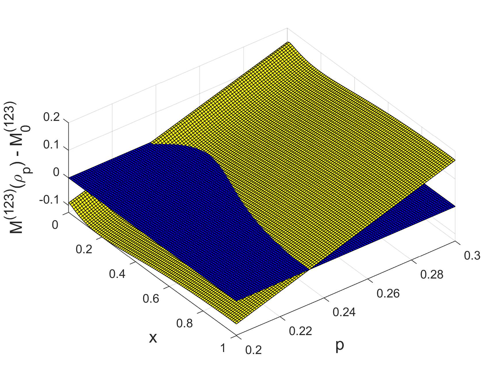
Choosing the Heisenberg-Weyl operators as the bases, we have $d_{1}=\kappa_{1}=3$ , $d_{2}=\kappa_{2}=3$ and $d_{3}=\kappa_{3}=2$ . Taking $\bm{u}=\left(x,x\right)^{\rm T}$ , $\bm{v}=\left(\sqrt{x},\sqrt{x}\right)^{\rm T}$ , $\bm{\alpha}=\left(-0.516382,-0.165015\right)^{\rm T}$ and $\bm{\beta}=\left(-0.259148,0.485242\right)^{\rm T}$ , by Theorem 3 we have that $\rho_{p}$ is genuinely tripartite entangled for $0.233233\leq p\leq 1$ . The result is shown in Figure 3, where the blue plane surface represents zero plane, the yellow curved surface represents the value of $M^{(123)}\left(\rho_{p}\right)-M^{(123)}_{0}$ .

We compare our result with those of Ref. Zhao et al. (2022b); Zhang et al. (2023) in Table 4, which shows that our criterion detects a wider genuine-tripartite-entanglement region.

Table 4: The comparison of detection thresholds for various criteria for the state

\rho_{p}

in Eq. (17).

Criteria	Range of $p$
Theorem 3	$0.233233\leq p\leq 1$
Zhang’s criterion Zhang et al. (2023)	$0.51<p\leq 1$
Zhao’s criterion Zhao et al. (2022b)	$0.5635<p\leq 1$

Concerning the fully separablity of $N$ -partite states, we have the following lemma, see proof in Appendix C.6.

Lemma 4.

If an $N$ -partite quantum state $\rho\in\mathcal{H}_{d_{1}}\otimes\cdots\otimes\mathcal{H}_{d_{N}}$ is fully separable, $\rho=\sum_{i}p_{i}\rho^{(1)}_{i}\otimes\cdots\otimes\rho^{(N)}_{i}$ , where $0\leq p_{i}\leq 1$ , $\sum_{i}p_{i}=1$ , $\rho^{(k)}_{i}$ is the pure state in the subsystem $\mathcal{H}_{d_{k}}$ , then for any $\left\{r_{1},\cdots,r_{k}\right\}\subseteq[N]$ , the correlation tensor $\mathcal{T}^{(r_{1}\cdots r_{k})}$ of the reduced state $\rho^{(r_{1}\cdots r_{k})}$ can be expressed as $\mathcal{T}^{(r_{1}\cdots r_{k})}=\sum_{i}p_{i}\mathcal{T}^{(r_{1})}_{i}\circ\cdots\circ\mathcal{T}^{(r_{k})}_{i}$ , where $\mathcal{T}^{(r_{l})}_{i}$ is the correlation tensor of the reduced state $\rho^{(r_{l})}_{i}$ , $l\in[k]$ .

The following corollary provides a criterion to detect the fully separability for multipartite states, which generalizes the Theorem 1 in Ref. Hassan and Joag (2008), see proof in Appendix C.7.

Corollary 1.

If an $N$ -partite quantum state $\rho\in\mathcal{H}_{d_{1}}\otimes\mathcal{H}_{d_{2}}\otimes\cdots\otimes\mathcal{H}_{d_{N}}$ is fully separable, then

\left\|\mathcal{T}^{(1\cdots N)}\right\|_{\rm tr}\leq\prod_{i=1}^{N}\sqrt{\frac{d_{i}^{2}-d_{i}}{\kappa_{i}}}.

Example 4.

Consider the following state Gittsovich et al. (2010),

\rho_{p,\epsilon}=\frac{1-p}{8}+p\ket{\psi_{\epsilon}}\bra{\psi_{\epsilon}},

(18)

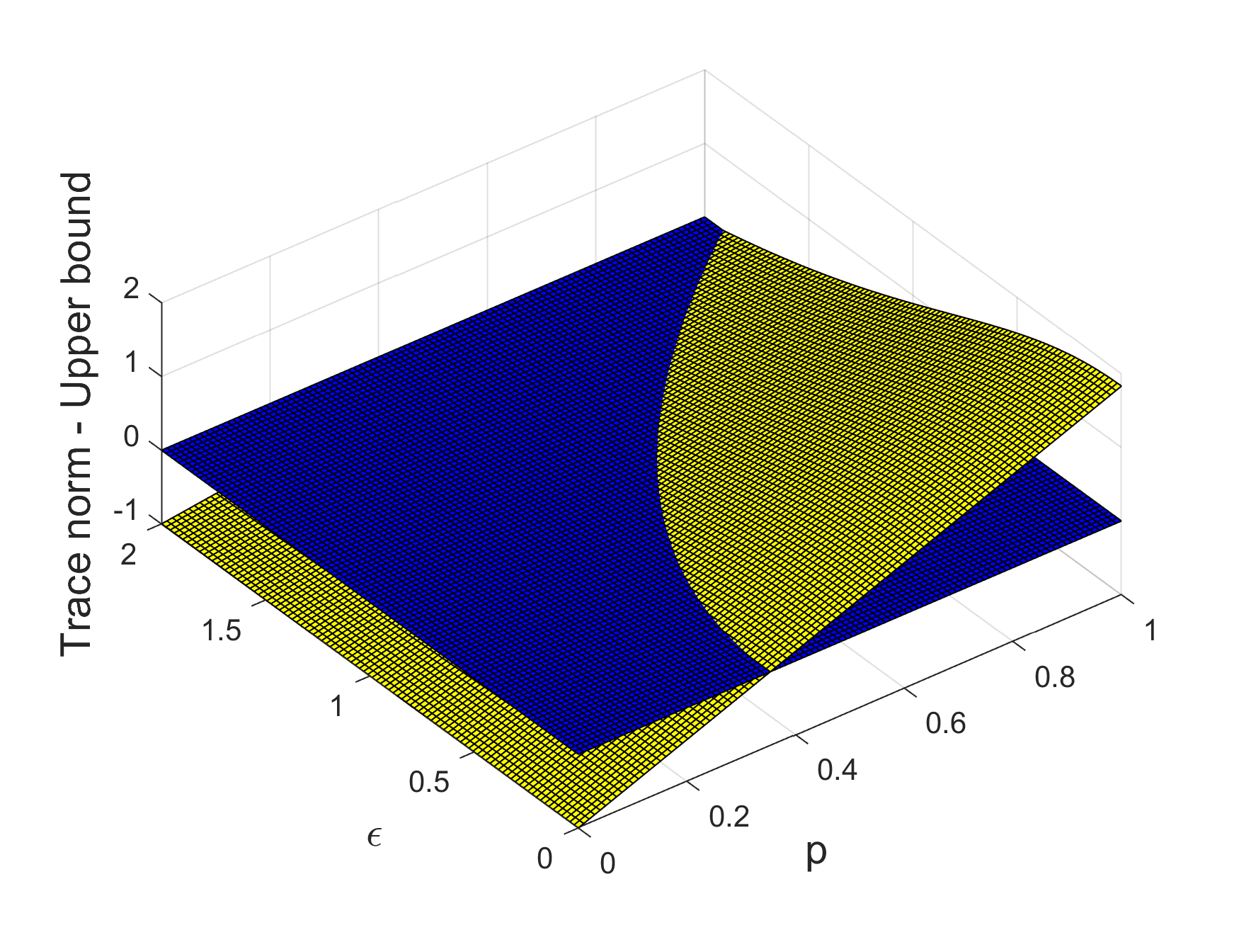
where $0\leq p\leq 1$ , $\ket{\psi_{\epsilon}}=\frac{1}{\sqrt{2+\epsilon^{2}}}\left(\ket{000}+\epsilon\ket{110}+\ket{111}\right)$ with real parameter $\epsilon$ . The dimensions of this state are $d_{1}=d_{2}=d_{3}=2$ . Choosing the Pauli operators as the bases gives that $\kappa_{1}=\kappa_{2}=\kappa_{3}=2$ . Corollary 1 shows that the state $\rho_{p,\epsilon}$ is entangled for the ranges of $p$ and $\epsilon$ shown in Figure 4, where the blue plane surface represents the zero plane, and the yellow curved surface represents the difference of the trace norm and the upper bound given in Corollary 1.

We compare our criterion with those in Ref. Zhang et al. (2017); Shen et al. (2022); Sun et al. (2025) for $\epsilon=10^{-1}$ and $\epsilon=1$ in Table 5, which implies that our criterion detects a wider range of entanglement for small $\epsilon$ .

Table 5: The comparison of detection thresholds for various criteria for the state

\rho_{p,\epsilon}

in Eq. (18).

$\epsilon$	$10^{-1}$	$1$
Zhang’s criterion Zhang et al. (2017)	$0.4118\leq p\leq 1$	$0.4256<p\leq 1$
Shen’s criterion Shen et al. (2022)	$0.4039\leq p\leq 1$	$0.4200<p\leq 1$
Sun’s criterion Sun et al. (2025)	$0.4026\leq p\leq 1$	$0.4194\leq p\leq 1$
Corollary 1	$0.355322\leq p\leq 1$	$0.53034\leq p\leq 1$

V Conclusions

In this work, we have established a unified and versatile framework for detecting entanglements in bipartite and multipartite quantum systems. At the core of this framework lies a novel extended correlation tensor constructed for bipartite states using the generalized Bloch representation, which incorporates adjustable parameters and allows flexibility in the choice of orthogonal basis. This design not only enhances the generality of the separability criterion but also bridges several existing criteria, such as those by de Vicente de Vicente (2007), Shen et al. Shen et al. (2016), Sarbicki et al. Sarbicki et al. (2020), Zhu et al. Zhu et al. (2023), and Huang et al. Huang et al. (2024), as special cases of our unified result.

To generalize the framework to multipartite systems, we adopt the technique of generalized matricization, specifically $\left(R,n;C,m\right)$ -mode matrix unfolding, which enables the systematic construction of extended correlation tensors under arbitrary bipartitions. This enabled us to derive practical criteria for both biseparability and full separability in multipartite states. Numerical experiments validated the effectiveness of our criteria, demonstrating enhanced detection capability over existing methods. Future works might be focused on establishing $k$ -separability criteria for general multipartite systems.

Declaration of competing interest

The authors declare no conflict of interest.

Data availability

No data was used for the research described in the article.

Acknowledgments

This work is supported by the Stable Supporting Fund of Acoustic Science and Technology Laboratory (Grant No. JCKYS2024604SSJS001) and the Fundamental Research Funds for the Central Universities (Grant No. 3072024XX2401).

Appendix A Several orthogonal basis

In this section, several orthogonal bases are presented, including Pauli operators, Weyl operators, and Heisenberg-Weyl operators.

Four $2$ -dimensional Pauli matrices are denoted as $\bm{\sigma}_{0}=\begin{pmatrix}1&0\\ 0&1\end{pmatrix}$ , $\bm{\sigma}_{1}=\begin{pmatrix}0&1\\ 1&0\end{pmatrix}$ , $\bm{\sigma}_{2}=\begin{pmatrix}0&-i\\ i&0\end{pmatrix}$ , $\bm{\sigma}_{3}=\begin{pmatrix}1&0\\ 0&-1\end{pmatrix}$ . And the explicit matrix representations of Pauli operators on the $2^{N}$ -dimensional Hilbert space are the tensor product of $N$ $2$ -dimensional Pauli matrices.

Let $\mathcal{H}$ be a $d$ -dimensional Hilbert space with computational basis $\left\{\ket{k}\right\}$ , and $\mathbb{Z}_{d}$ denote the finite field of modulo $d$ integers. The Weyl operators are defined by $\mathbf{W}\left(n,m\right)=\sum_{k\in\mathbb{Z}_{d}}e^{\frac{2kn\pi i}{d}}\ket{k}\bra{(k+m)\text{mod }d}$ , where $n,m\in[0,d-1]$ . The set $\left\{\mathbf{W}\left(n,m\right)\right\}$ forms the basis for linear generators in the general linear Lie algebra $\mathfrak{gl}(d)$ Huang et al. (2022). If $d=2$ , the Weyl operators are equal to the $2$ -dimensional Pauli operators.

The $d$ -dimensional Heisenberg-Weyl operators Asadian et al. (2016); Chang et al. (2018) are defined by $\mathbf{Q}\left(l,m\right)=\chi\mathbf{W}\left(n,m\right)+\chi^{*}\mathbf{W}^{\dagger}\left(l,m\right)$ , where $\chi=\left(1+i\right)/2$ .

Appendix B Matrix unfolding of tensors

In special cases, the ${(R,n;C,m)}$ -mode matrix unfolding can reduce to the vectorization or the matrix unfolding of Ref. De Lathauwer et al. (2000), as shown in Table 6.

$R$	$n$	$C$	$m$	$\mathbf{A}_{(R,n;C,m)}$
$[N]$	$n$	$\emptyset$	/	$\operatorname{vec}_{n}\left(\mathcal{A}\right)$
$\emptyset$	/	$[N]$	$m$	$\operatorname{vec}_{m}^{\rm T}\left(\mathcal{A}\right)$
$\left\{r_{1}\right\}$	$1$	$[N]\setminus\left\{r_{1}\right\}$	$N-1$	$\mathbf{A}_{(r_{1})}$
$[N]\setminus\left\{c_{1}\right\}$	$N-1$	$\left\{c_{1}\right\}$	$1$	$\mathbf{A}_{(c_{1})}^{\rm T}$

Table 6: The reduction from the

(R,n;C,m)

-mode matrix unfolding to the vectorization or the matrix unfolding of Ref. De Lathauwer et al. (2000) for a tensor

\mathcal{A}\in\mathbb{C}^{d_{1}\times\cdots\times d_{N}}

in special cases.

The process of the $\left(R,n;C,m\right)$ -mode matrix unfolding of tensors can be visually decomposed into the following three steps:

•

Step 1: A tensor $\mathcal{A}=\left(a_{i_{1}\cdots i_{N}}\right)\in\mathbb{C}^{d_{1}\times\cdots\times d_{N}}$ can be considered as a special “tensor” $\tilde{\mathcal{A}}=\left(\tilde{a}_{i_{r_{1}}\cdots i_{r_{k}}}\right)$ of size $d_{r_{1}}\times\cdots\times d_{r_{k}}$ , whose entries $\tilde{a}_{i_{r_{1}}\cdots i_{r_{k}}}$ are sub-tensors of size $d_{c_{1}}\times\cdots\times d_{c_{N-k}}$ .
•

Step 2: Performing the $n$ -mode vectorization to $\tilde{\mathcal{A}}$ yields a “column vector” ${\rm vec}_{n}\left(\tilde{\mathcal{A}}\right)$ , whose entries $\tilde{a}_{i}$ have size $d_{c_{1}}\times\cdots\times d_{c_{N-k}}$ for $i\in[d_{r_{1}}\cdots d_{r_{k}}]$ .
•

Step 3: Perform the $m$ -mode vectorization to all entries $\tilde{a}_{j}$ and then transpose them, respectively.

During the expansion process, the rows are first processed, followed by the columns. Alternatively, $\mathcal{A}$ can be viewed as a special “tensor” $\tilde{\mathcal{A}}^{\prime}$ of size $d_{c_{1}}\times\cdots\times d_{c_{N-k}}$ , where each entry is a sub-tensor of size $d_{r_{1}}\times\cdots\times d_{r_{k}}$ . In this alternative approach, the columns are processed first, followed by the rows. Both approaches yield the same matrix.

The following theorem gives the relation between the $\left(R,n;C,m\right)$ -mode matrix unfolding of tensors with the outer product.

Theorem 4.

Given two tensors $\mathcal{A}\in\mathbb{C}^{d_{1}\times\cdots\times d_{k}}$ , $\mathcal{B}\in\mathbb{C}^{d_{k+1}\times\cdots\times d_{N}}$ with $k\in[N-1]$ , let $\mathcal{C}=\mathcal{A}\circ\mathcal{B}$ and $R=\left\{r_{1},\cdots,r_{k}\right\},C=\left\{c_{1},\cdots,c_{N-k}\right\}$ be two disjoint ascending ordered sets with $R\cup C=[N]$ . Then, for any $n\in[k]$ and $m\in[N-k]$ , we have

\mathbf{C}_{\left(R,n;C,m\right)}={\rm vec}_{n}\left(\mathcal{A}\right){\rm vec}_{m}^{\rm T}\left(\mathcal{B}\right).

Proof.

Let $\mathcal{A}=\sum_{i_{1},\cdots,i_{k}}a_{i_{1}\cdots i_{k}}\bm{e}^{(1)}_{i_{1}}\circ\cdots\circ\bm{e}^{(k)}_{i_{k}}$ and $\mathcal{B}=\sum_{i_{k+1},\cdots,i_{N}}b_{i_{k+1}\cdots i_{N}}\bm{e}^{(k+1)}_{i_{k+1}}\circ\cdots\circ\bm{e}^{(N)}_{i_{N}}$ . Then $\mathcal{C}=\mathcal{A}\circ\mathcal{B}=\sum_{i_{1},\cdots,i_{N}}a_{i_{1}\cdots i_{k}}b_{i_{k+1}\cdots i_{N}}\bm{e}^{(1)}_{i_{1}}\circ\cdots\circ\bm{e}^{(N)}_{i_{N}}$ . Therefore, we have

		$\displaystyle\mathbf{C}_{\left(R,n;C,m\right)}$
	$\displaystyle=$	$\displaystyle\sum_{i_{1},\cdots,i_{N}}a_{i_{1}\cdots i_{k}}b_{i_{k+1}\cdots i_{N}}\left(\left(\bigotimes_{i=n+1}^{k}\bm{e}^{(i)}\right)\otimes\left(\bigotimes_{i=1}^{n}\bm{e}^{(i)}\right)\right)$
		$\displaystyle\cdot\left(\left(\bigotimes_{i=m+1}^{N-k}\bm{e}^{(k+i)}\right)\otimes\left(\bigotimes_{i=1}^{m}\bm{e}^{(k+i)}\right)\right)^{\rm T}$
	$\displaystyle=$	$\displaystyle\left(\sum_{i_{1},\cdots,i_{k}}a_{i_{1}\cdots i_{k}}\left(\bigotimes_{i=n+1}^{k}\bm{e}^{(i)}\right)\otimes\left(\bigotimes_{i=1}^{n}\bm{e}^{(i)}\right)\right)$
		$\displaystyle\cdot\left(\sum_{i_{k+1},\cdots,i_{N}}b_{i_{k+1}\cdots i_{N}}\left(\bigotimes_{i=m+1}^{N-k}\bm{e}^{(k+i)}\right)\otimes\left(\bigotimes_{i=1}^{m}\bm{e}^{(k+i)}\right)\right)^{\rm T}$
	$\displaystyle=$	$\displaystyle\operatorname{vec}_{n}\left(\mathcal{A}\right)\operatorname{vec}_{m}^{\rm T}\left(\mathcal{B}\right)$

∎

Appendix C Proof of Lemmas and Theorems

C.1 Proof of Theorem 1

Proof.

Since $\rho^{(AB)}$ is separable, it can be expressed as a convex combination of product states,

\rho^{(AB)}=\sum_{i}p_{i}\rho^{(A)}_{i}\otimes\rho^{(B)}_{i},

(19)

where $0\leq p_{i}\leq 1$ , $\sum_{i}p_{i}=1$ , $\rho^{(A)}_{i}$ and $\rho^{(B)}_{i}$ are pure states in $\mathcal{H}_{d_{A}}$ and $\mathcal{H}_{d_{B}}$ , respectively.

By the generalized Bloch representation of $\rho^{(A)}_{i},\rho^{(B)}_{i}$ in Eq (1), there exist vectors $\mathcal{T}^{(A)}_{i}\in\mathbb{C}^{d_{A}^{2}-1}$ , $\mathcal{T}^{(B)}_{i}\in\mathbb{C}^{d_{B}^{2}-1}$ such that $\mathcal{T}^{(A)}=\sum_{i}p_{i}\mathcal{T}^{(A)}_{i}$ , $\mathcal{T}^{(B)}=\sum_{i}p_{i}\mathcal{T}^{(B)}_{i}$ . According to Lemma 1, we have $\left\|\mathcal{T}^{(A)}_{i}\right\|_{F}^{2}\leq\frac{d_{A}^{2}-d_{A}}{\kappa_{A}}$ , $\left\|\mathcal{T}^{(B)}_{i}\right\|_{F}^{2}\leq\frac{d_{B}^{2}-d_{B}}{\kappa_{B}}$ .

Substituting the generalized Bloch representation of $\rho^{(AB)}$ in Eq. (4) and the generalized Bloch representations of $\rho^{(A)}_{i},\rho^{(B)}_{i}$ in Eq. (1) into Eq. (19), we derive that $\mathcal{T}^{(AB)}=\sum_{i}{p_{i}}\mathcal{T}^{(A)}_{i}\left(\mathcal{T}^{(B)}_{i}\right)^{\rm T}$ .

Therefore, we obtain that

		$\displaystyle\left\\|\mathcal{M}_{\bm{u},\bm{v},\bm{\alpha},\bm{\beta}}^{(A\|B)}(\rho^{(AB)})\right\\|_{\rm tr}$
	$\displaystyle=$	$\displaystyle\left\\|\begin{pmatrix}\bm{u}\bm{v}^{\rm T}&\bm{u}\left(\bm{\beta}\otimes\mathcal{T}^{(B)}\right)^{\rm T}\\ \left(\bm{\alpha}\otimes\mathcal{T}^{(A)}\right)\bm{v}^{\rm T}&\bm{\alpha}\bm{\beta}^{\rm T}\otimes\mathcal{T}^{(AB)}\\ \end{pmatrix}\right\\|_{\rm tr}$
	$\displaystyle=$	$\displaystyle\left\\|\begin{pmatrix}\bm{u}\bm{v}^{\rm T}&\bm{u}\left(\bm{\beta}\otimes\sum_{i}p_{i}\mathcal{T}^{(B)}_{i}\right)^{\rm T}\\ \left(\bm{\alpha}\otimes\sum_{i}p_{i}\mathcal{T}^{(A)}_{i}\right)\bm{v}^{\rm T}&\bm{\alpha}\bm{\beta}^{\rm T}\otimes\left(\sum_{i}{p_{i}}\mathcal{T}^{(A)}_{i}\left(\mathcal{T}^{(B)}_{i}\right)^{\rm T}\right)\\ \end{pmatrix}\right\\|_{\rm tr}$
	$\displaystyle\leq$	$\displaystyle\sum_{i}p_{i}\left\\|\begin{pmatrix}\bm{u}\bm{v}^{\rm T}&\bm{u}\left(\bm{\beta}\otimes\mathcal{T}^{(B)}_{i}\right)^{\rm T}\\ \left(\bm{\alpha}\otimes\mathcal{T}^{(A)}_{i}\right)\bm{v}^{\rm T}&\bm{\alpha}\bm{\beta}^{\rm T}\otimes\left(\mathcal{T}^{(A)}_{i}\left(\mathcal{T}^{(B)}_{i}\right)^{\rm T}\right)\\ \end{pmatrix}\right\\|_{\rm tr}$
	$\displaystyle\leq$	$\displaystyle\sum{p_{i}}\left\\|\begin{pmatrix}\bm{u}\\ \bm{\alpha}\otimes\mathcal{T}^{(A)}_{i}\\ \end{pmatrix}\right\\|_{\rm tr}\left\\|\begin{pmatrix}\bm{v}^{\rm T}&\left(\bm{\beta}\otimes\mathcal{T}^{(B)}_{i}\right)^{\rm T}\end{pmatrix}\right\\|_{\rm tr}$
	$\displaystyle\leq$	$\displaystyle\sqrt{\left(\left\\|\bm{u}\right\\|_{F}^{2}+\left\\|\bm{\alpha}\right\\|_{F}^{2}\frac{{d_{A}}^{2}-d_{A}}{\kappa_{A}}\right)\left(\left\\|\bm{v}\right\\|_{F}^{2}+\left\\|\bm{\beta}\right\\|_{F}^{2}\frac{{d_{B}}^{2}-d_{B}}{\kappa_{B}}\right)}.$

∎

C.2 Proof of Lemma 2

Proof.

Denote $\rho^{(1\cdots N)}$ the state in $\mathcal{H}_{d_{1}}\otimes\cdots\otimes\mathcal{H}_{d_{N}}$ of the multipartite system. By the generalized Bloch representation in Eq. (12) and the condition in Eq. (11), we obtain that

	$\displaystyle{\rm Tr}\left(\left(\rho^{(1\cdots N)}\right)^{2}\right)$	(20)
$\displaystyle=$	$\displaystyle{\rm Tr}\left(\left(\rho^{(1\cdots N)}\right)^{\dagger}\rho^{(1\cdots N)}\right)$
$\displaystyle=$	$\displaystyle\frac{1}{d_{1}^{2}\cdots d_{N}^{2}}\left(d_{1}\cdots d_{N}\right.$
	$\displaystyle+\kappa_{1}d_{2}\cdots d_{N}\left\\|\mathcal{T}^{(1)}\right\\|_{F}^{2}+\cdots+\kappa_{N}d_{1}\cdots d_{N-1}\left\\|\mathcal{T}^{(N)}\right\\|_{F}^{2}$
	$\displaystyle+\kappa_{1}\kappa_{2}d_{3}\cdots d_{N}\left\\|\mathcal{T}^{(12)}\right\\|_{F}^{2}+\cdots$
	$\displaystyle+\kappa_{N-1}\kappa_{N}d_{1}\cdots d_{N-2}\left\\|\mathcal{T}^{(N-1N)}\right\\|_{F}^{2}$
	$\displaystyle\left.+\cdots+\kappa_{1}\cdots\kappa_{N}\left\\|\mathcal{T}^{(1\cdots N)}\right\\|_{F}^{2}\right)$
$\displaystyle=$	$\displaystyle\frac{1}{d_{1}\cdots d_{N}}\left(1+A_{1}^{(1\cdots N)}+A_{2}^{(1\cdots N)}+\cdots+A_{N}^{(1\cdots N)}\right),$

where

\begin{gathered}A_{1}^{(1\cdots N)}=\frac{\kappa_{1}}{d_{1}}\left\|\mathcal{T}^{(1)}\right\|_{F}^{2}+\cdots+\frac{\kappa_{N}}{d_{N}}\left\|\mathcal{T}^{(N)}\right\|_{F}^{2},\\ A_{2}^{(1\cdots N)}=\frac{\kappa_{1}\kappa_{2}}{d_{1}d_{2}}\left\|\mathcal{T}^{(12)}\right\|_{F}^{2}+\cdots+\frac{\kappa_{N-1}\kappa_{N}}{d_{N-1}d_{N}}\left\|\mathcal{T}^{(N-1N)}\right\|_{F}^{2},\\ \cdots,\\ A_{n}^{(1\cdots N)}=\frac{\kappa_{1}\cdots\kappa_{N}}{d_{1}\cdots d_{N}}\left\|\mathcal{T}^{(1\cdots N)}\right\|_{F}^{2}.\end{gathered}

Let $\rho^{(j_{1})}$ and $\rho^{(j_{2}\cdots j_{N})}$ be the reduced states of $\rho^{(1\cdots N)}$ with respect to the subsystems $\mathcal{H}_{d_{j_{1}}}$ and $\mathcal{H}_{d_{j_{2}}}\otimes\cdots\otimes\mathcal{H}_{d_{j_{N}}}$ , respectively, where $\left\{j_{1},j_{2},\cdots,j_{N}\right\}=[N]$ .

If $\rho^{(1\cdots N)}$ is pure state, we have

	$\displaystyle{\rm Tr}\left(\left(\rho^{(1\cdots N)}\right)^{2}\right)$	(21)
$\displaystyle=$	$\displaystyle\frac{1}{d_{1}\cdots d_{N}}\left(1+A_{1}^{(1\cdots N)}+A_{2}^{(1\cdots N)}+\cdots+A_{N}^{(1\cdots N)}\right)$
$\displaystyle=$	$\displaystyle 1,$

and

{\rm Tr}\left(\left(\rho^{(j_{1})}\right)^{2}\right)={\rm Tr}\left(\left(\rho^{(j_{2}\cdots j_{N})}\right)^{2}\right),

(22)

which follows that

\sum_{j_{1}=1}^{N}\frac{1}{d_{j_{1}}}{\rm Tr}\left(\left(\rho^{(j_{1})}\right)^{2}\right)=\sum_{j_{1}=1}^{N}\frac{1}{d_{j_{1}}}{\rm Tr}\left(\left(\rho^{(j_{2}\cdots j_{N})}\right)^{2}\right).

(23)

On one hand, $\rho^{(j_{1})}$ is computed by performing the partial trace to $\rho^{(1\cdots N)}$ , that is,

\rho^{(j_{1})}={\rm Tr}_{j_{2}\cdots j_{N}}\left(\rho^{(1\cdots N)}\right)=\frac{1}{d_{j_{1}}}\left(\mathbf{I}_{d_{j_{1}}}^{(j_{1})}+\sum_{i_{j_{1}}=1}^{d_{j_{1}}^{2}-1}t_{i_{j_{1}}}^{(j_{1})}\mathbf{G}_{i_{j_{1}}}^{(j_{1})}\right).

Then we have

	$\displaystyle\sum_{j_{1}=1}^{N}\frac{1}{d_{j_{1}}}{\rm Tr}\left(\left(\rho^{(j_{1})}\right)^{2}\right)$	(24)
$\displaystyle=$	$\displaystyle\sum_{j_{1}=1}^{N}\frac{1}{d_{j_{1}}}\left(\frac{1}{d_{j_{1}}^{2}}\left(d_{j_{1}}+\kappa_{j_{1}}\left\\|\mathcal{T}^{(j_{1})}\right\\|_{F}^{2}\right)\right)$
$\displaystyle=$	$\displaystyle\sum_{j_{1}=1}^{N}\frac{1}{d_{j_{1}}^{2}}+\sum_{j_{1}=1}^{N}\frac{\kappa_{j_{1}}}{d_{j_{1}}^{3}}\left\\|\mathcal{T}^{(j_{1})}\right\\|_{F}^{2}.$

On the other hand, according to Eq. (20), we obtain that

	$\displaystyle\sum_{j_{1}=1}^{N}\frac{1}{d_{j_{1}}}{\rm Tr}\left(\left(\rho^{(j_{2}\cdots j_{N})}\right)^{2}\right)$	(25)
$\displaystyle=$	$\displaystyle\frac{1}{d_{1}}{\rm Tr}\left(\left(\rho^{(2\cdots N)}\right)^{2}\right)+\frac{1}{d_{2}}{\rm Tr}\left(\left(\rho^{(13\cdots N)}\right)^{2}\right)$
	$\displaystyle+\cdots+\frac{1}{d_{N}}{\rm Tr}\left(\left(\rho^{(1\cdots N-1)}\right)^{2}\right)$
$\displaystyle=$	$\displaystyle\frac{1}{d_{1}\cdots d_{N}}\left(N+\left(A_{1}^{(2\cdots N)}+A_{1}^{(13\cdots N)}+\cdots+A_{1}^{(1\cdots N-1)}\right)\right.$
	$\displaystyle+\left(A_{2}^{(2\cdots N)}+A_{2}^{(13\cdots N)}+\cdots+A_{2}^{(1\cdots N-1)}\right)$
	$\displaystyle\left.+\cdots+\left(A_{N-1}^{(2\cdots N)}+A_{N-1}^{(13\cdots N)}+\cdots+A_{N-1}^{(1\cdots N-1)}\right)\right)$
$\displaystyle=$	$\displaystyle\frac{1}{d_{1}\cdots d_{N}}\left(N+\left(N-1\right)A_{1}^{(1\cdots N)}+\left(N-2\right)A_{2}^{(1\cdots N)}\right.$
	$\displaystyle\left.+\cdots+A_{N-1}^{(1\cdots N)}\right).$

Substituting Eq. (24) and (25) into Eq. (21), we have

	$\displaystyle\sum_{i=1}^{N}\frac{1}{d_{i}^{2}}+\sum_{i=1}^{N}\frac{\kappa_{i}}{d_{i}^{3}}\left\\|\mathcal{T}^{(i)}\right\\|_{F}^{2}$	(26)
$\displaystyle=$	$\displaystyle\frac{1}{d_{1}\cdots d_{N}}\left(N+\left(N-1\right)A_{1}^{(1\cdots N)}+\left(N-2\right)A_{2}^{(1\cdots N)}\right.$
	$\displaystyle\left.+\cdots+A_{N-1}^{(1\cdots N)}\right).$

Case 1: $N=1$ .

By Lemma 1, we have $\left\|\mathcal{T}^{(1)}\right\|_{F}^{2}\leq\frac{d_{1}^{2}-d_{1}}{\kappa_{1}}$ .

Case 2: $N=2$ or $N\geq 3$ , $\frac{d_{1}\cdots d_{N}}{d^{2}}<1$ .

Since $\left\|\mathcal{T}^{(i)}\right\|_{F}^{2}\geq 0$ , we have

		$\displaystyle\sum_{i=1}^{N}\frac{1}{d_{i}^{2}}$
	$\displaystyle\leq$	$\displaystyle\frac{1}{d_{1}\cdots d_{N}}\left(N+\left(N-1\right)\left(A_{1}^{(1\cdots N)}+A_{2}^{(1\cdots N)}\right.\right.$
		$\displaystyle\left.\left.+\cdots+A_{N-1}^{(1\cdots N)}\right)\right)$
	$\displaystyle=$	$\displaystyle\frac{1}{d_{1}\cdots d_{N}}\left(N+\left(N-1\right)\left(d_{1}\cdots d_{N}-1-A_{N}^{(1\cdots N)}\right)\right),$

that is,

		$\displaystyle\left\\|\mathcal{T}^{(1\cdots N)}\right\\|_{F}^{2}$
	$\displaystyle\leq$	$\displaystyle\frac{d_{1}\cdots d_{N}}{\kappa_{1}\cdots\kappa_{N}}\left(d_{1}\cdots d_{N}+\frac{1}{N-1}-\frac{d_{1}\cdots d_{N}}{N-1}\sum_{i=1}^{N}\frac{1}{d_{i}^{2}}\right).$

Case 3: $N\geq 3$ , $\frac{d_{1}\cdots d_{N}}{d^{2}}\geq 1$ .

Since $d=\max_{i\in[N]}\left\{d_{i}\right\}$ and $\frac{d_{1}\cdots d_{N}}{d^{2}}\geq 1$ , we have

		$\displaystyle\sum_{j_{1}=1}^{N}\frac{1}{d_{j_{1}}^{2}}+\sum_{j_{1}=1}^{N}\frac{\kappa_{j_{1}}}{d_{j_{1}}^{3}}\left\\|\mathcal{T}^{(j_{1})}\right\\|_{F}^{2}$
	$\displaystyle\geq$	$\displaystyle\sum_{j_{1}=1}^{N}\frac{1}{d_{j_{1}}^{2}}+\frac{1}{d^{2}}\sum_{j_{1}=1}^{N}\frac{\kappa_{j_{1}}}{d_{j_{1}}}\left\\|\mathcal{T}^{(j_{1})}\right\\|_{F}^{2}$
	$\displaystyle\geq$	$\displaystyle\sum_{j_{1}=1}^{N}\frac{1}{d_{j_{1}}^{2}}+\frac{1}{d_{1}\cdots d_{N}}A^{(1\cdots N)}_{1},$

Then we obtain that

		$\displaystyle\sum_{j_{1}=1}^{N}\frac{1}{d_{j_{1}}^{2}}+\frac{1}{d_{1}\cdots d_{N}}A^{(1\cdots N)}_{1}$
	$\displaystyle\leq$	$\displaystyle\frac{1}{d_{1}\cdots d_{N}}\left(N+\left(N-1\right)A_{1}^{(1\cdots N)}\right.$
		$\displaystyle\left.+\left(N-2\right)\left(A_{2}^{(1\cdots N)}+\cdots+A_{N-1}^{(1\cdots N)}\right)\right),$

that is,

		$\displaystyle\frac{d_{1}\cdots d_{N}}{N-2}\sum_{j_{1}=1}^{N}\frac{1}{d_{j_{1}}^{2}}$
	$\displaystyle\leq$	$\displaystyle\frac{N}{N-2}+A_{1}^{(1\cdots N)}+A_{2}^{(1\cdots N)}+\cdots+A_{N-1}^{(1\cdots N)}$
	$\displaystyle=$	$\displaystyle\frac{2}{N-2}+d_{1}\cdots d_{N}-A^{(1\cdots N)}_{N},$

which follows that

		$\displaystyle\left\\|\mathcal{T}^{(1\cdots N)}\right\\|_{F}^{2}$
	$\displaystyle\leq$	$\displaystyle\frac{d_{1}\cdots d_{N}}{\kappa_{1}\cdots\kappa_{N}}\left(d_{1}\cdots d_{N}+\frac{2}{N-2}-\frac{d_{1}\cdots d_{N}}{N-2}\sum_{i=1}^{N}\frac{1}{d_{i}^{2}}\right).$

Thus, by the above three cases, it holds that

\left\|\mathcal{T}^{(1\cdots N)}\right\|_{F}^{2}\leq\mathfrak{m}^{(1\cdots N)}.

If $\rho^{(1\cdots N)}$ is a mixed state, then it can be represented as a convex combination of pure states, that is, $\rho^{(1\cdots N)}=\sum_{i}p_{i}\rho_{i}^{(1\cdots N)}$ , where $0\leq p_{i}\leq 1$ , $\sum_{i}p_{i}=1$ . Therefore, by the convexity of the Frobenius norm, we obtain that

	$\displaystyle\left\\|\mathcal{T}^{(1\cdots N)}\right\\|_{F}^{2}=\left\\|\sum_{i}p_{i}\mathcal{T}^{(1\cdots N)}_{i}\right\\|_{F}^{2}\leq$	$\displaystyle\sum_{i}p_{i}\left\\|\mathcal{T}^{(1\cdots N)}_{i}\right\\|_{F}^{2}$
	$\displaystyle\leq$	$\displaystyle\mathfrak{m}^{(1\cdots N)},$

where $\mathcal{T}^{(1\cdots N)}_{i}$ is the correlation tensor of $\rho_{i}^{(1\cdots N)}$ . ∎

C.3 Proof of Lemma 3

Proof.

Suppose that $\left\{l_{1},\cdots,l_{k}\right\}\setminus\left\{r_{1},\cdots,r_{p}\right\}=\left\{r_{p+1},\cdots,r_{k}\right\}$ and $\left\{l_{k+1},\cdots,l_{N}\right\}\setminus\left\{c_{1},\cdots,c_{q}\right\}=\left\{c_{q+1},\cdots,c_{N-k}\right\}$ . Then we have

	$\displaystyle\rho^{(r_{1}\cdots r_{p}c_{1}\cdots c_{q})}$	(27)
$\displaystyle=$	$\displaystyle{\rm Tr}_{r_{p+1}\cdots r_{k}c_{q+1}\cdots c_{N-k}}\left(\rho\right)$
$\displaystyle=$	$\displaystyle{\rm Tr}_{r_{p+1}\cdots r_{k}c_{q+1}\cdots c_{N-k}}\left(\sum_{i}p_{i}\rho^{(l_{1}\cdots l_{k})}_{i}\otimes\rho^{(l_{k+1}\cdots l_{N})}_{i}\right)$
$\displaystyle=$	$\displaystyle\sum_{i}p_{i}{\rm Tr}_{r_{p+1}\cdots r_{k}}\left(\rho^{(l_{1}\cdots l_{k})}_{i}\right)\otimes{\rm Tr}_{c_{q+1}\cdots c_{N-k}}\left(\rho^{(l_{k+1}\cdots l_{N})}_{i}\right)$
$\displaystyle=$	$\displaystyle\sum_{i}p_{i}\rho^{(r_{1}\cdots r_{p})}_{i}\otimes\rho^{(c_{1}\cdots c_{q})}_{i}.$

By the generalized Bloch representation in Eq. (12), $\rho^{(r_{1}\cdots r_{p})}_{i}$ , and $\rho^{(c_{1}\cdots c_{q})}_{i}$ can be expanded as

	$\displaystyle\rho^{(r_{1}\cdots r_{p})}_{i}$	(28)
$\displaystyle=$	$\displaystyle\frac{1}{d_{r_{1}}\cdots d_{r_{p}}}\left(\mathbf{I}_{d_{r_{1}}}^{(r_{1})}\otimes\cdots\otimes\mathbf{I}_{d_{r_{p}}}^{(r_{p})}+\cdots\right.$
	$\displaystyle\left.+\sum_{i_{r_{1}},\cdots,i_{r_{p}}=1}^{d_{r_{1}}^{2}-1,\cdots,d_{r_{p}}^{2}-1}t_{i_{r_{1}}\cdots i_{r_{p}}}^{(i,r_{1}\cdots r_{p})}\mathbf{G}_{i_{r_{1}}}^{(r_{1})}\otimes\cdots\otimes\mathbf{G}_{i_{r_{p}}}^{(r_{p})}\right),$

	$\displaystyle\rho^{(c_{1}\cdots c_{q})}_{i}$	(29)
$\displaystyle=$	$\displaystyle\frac{1}{d_{c_{1}}\cdots d_{c_{q}}}\left(\mathbf{I}_{d_{c_{1}}}^{(c_{1})}\otimes\cdots\otimes\mathbf{I}_{d_{c_{q}}}^{(c_{q})}+\cdots\right.$
	$\displaystyle\left.+\sum_{i_{c_{1}},\cdots,i_{c_{q}}=1}^{d_{c_{1}}^{2}-1,\cdots,d_{c_{q}}^{2}-1}t_{i_{c_{1}}\cdots i_{c_{q}}}^{(i,c_{1}\cdots c_{q})}\mathbf{G}_{i_{c_{1}}}^{(c_{1})}\otimes\cdots\otimes\mathbf{G}_{i_{c_{q}}}^{(c_{q})}\right),$

where $\mathcal{T}^{(r_{1}\cdots r_{p})}_{i}=\left(t_{i_{r_{1}}\cdots i_{r_{p}}}^{(i,r_{1}\cdots r_{p})}\right)$ and $\mathcal{T}^{(c_{1}\cdots c_{q})}_{i}=\left(t_{i_{c_{1}}\cdots i_{c_{q}}}^{(i,c_{1}\cdots c_{q})}\right)$ are the correlation tensors of $\rho^{(r_{1}\cdots r_{p})}_{i}$ and $\rho^{(c_{1}\cdots c_{q})}_{i}$ , respectively. Substituting Eq. (28) and (29) into Eq. (27), we have

	$\displaystyle\rho^{(r_{1}\cdots r_{p}c_{1}\cdots c_{q})}$	(30)
$\displaystyle=$	$\displaystyle\frac{1}{d_{r_{1}}\cdots d_{r_{p}}d_{c_{1}}\cdots d_{c_{q}}}\sum_{i}p_{i}$
	$\displaystyle\cdot\left(\mathbf{I}_{d_{r_{1}}}^{(r_{1})}\otimes\cdots\otimes\mathbf{I}_{d_{r_{p}}}^{(r_{p})}\otimes\mathbf{I}_{d_{c_{1}}}^{(c_{1})}\otimes\cdots\otimes\mathbf{I}_{d_{c_{q}}}^{(c_{q})}+\cdots\right.$
	$\displaystyle+\sum_{i_{r_{1}},\cdots,i_{r_{p}}=1}^{d_{r_{1}}^{2}-1,\cdots,d_{r_{p}}^{2}-1}\sum_{i_{c_{1}},\cdots,i_{c_{q}}=1}^{d_{c_{1}}^{2}-1,\cdots,d_{c_{q}}^{2}-1}t_{i_{r_{1}}\cdots i_{r_{p}}}^{(i,r_{1}\cdots r_{p})}t_{i_{c_{1}}\cdots i_{c_{q}}}^{(i,c_{1}\cdots c_{q})}$
	$\displaystyle\left.\cdot\mathbf{G}_{i_{r_{1}}}^{(r_{1})}\otimes\cdots\otimes\mathbf{G}_{i_{r_{p}}}^{(r_{p})}\otimes\mathbf{G}_{i_{c_{1}}}^{(c_{1})}\otimes\cdots\otimes\mathbf{G}_{i_{c_{q}}}^{(c_{q})}\right).$

By the generalized Bloch representation of $\rho$ in Eq. (12), $\rho_{r_{1}\cdots r_{p}c_{1}\cdots c_{q}}$ can be computed as follows,

	$\displaystyle\rho^{(r_{1}\cdots r_{p}c_{1}\cdots c_{q})}$	(31)
$\displaystyle=$	$\displaystyle{\rm Tr}_{r_{p+1}\cdots r_{k}c_{q+1}\cdots c_{N-k}}\left(\rho\right)$
$\displaystyle=$	$\displaystyle\frac{1}{d_{r_{1}}\cdots d_{r_{p}}d_{c_{1}}\cdots d_{c_{q}}}$
	$\displaystyle\cdot\left(\mathbf{I}_{d_{r_{1}}}^{(r_{1})}\otimes\cdots\otimes\mathbf{I}_{d_{r_{p}}}^{(r_{p})}\otimes\mathbf{I}_{d_{c_{1}}}^{(c_{1})}\otimes\cdots\otimes\mathbf{I}_{d_{c_{q}}}^{(c_{q})}+\cdots\right.$
	$\displaystyle+\sum_{i_{r_{1}},\cdots,i_{r_{p}}=1}^{d_{r_{1}}^{2}-1,\cdots,d_{r_{p}}^{2}-1}\sum_{i_{c_{1}},\cdots,i_{c_{q}}=1}^{d_{c_{1}}^{2}-1,\cdots,d_{c_{q}}^{2}-1}t_{i_{r_{1}}\cdots i_{r_{p}}i_{c_{1}}\cdots i_{c_{q}}}^{(r_{1}\cdots r_{p}c_{1}\cdots c_{q})}$
	$\displaystyle\left.\cdot\mathbf{G}_{i_{r_{1}}}^{(r_{1})}\otimes\cdots\otimes\mathbf{G}_{i_{r_{p}}}^{(r_{p})}\otimes\mathbf{G}_{i_{c_{1}}}^{(c_{1})}\otimes\cdots\otimes\mathbf{G}_{i_{c_{q}}}^{(c_{q})}\right),$

where $\mathcal{T}^{(r_{1}\cdots r_{p}c_{1}\cdots c_{q})}=\left(t_{i_{r_{1}}\cdots i_{r_{p}}i_{c_{1}}\cdots i_{c_{q}}}^{(r_{1}\cdots r_{p}c_{1}\cdots c_{q})}\right)$ is the correlation tensor of $\rho^{(r_{1}\cdots r_{p}c_{1}\cdots c_{q})}$ .

Comparing Eq. (30) with Eq. (31), we see that

\begin{gathered}t_{i_{r_{1}}\cdots i_{r_{p}}i_{c_{1}}\cdots i_{c_{q}}}^{(r_{1}\cdots r_{p}c_{1}\cdots c_{q})}=\sum_{i}p_{i}t_{i_{r_{1}}\cdots i_{r_{p}}}^{(i,r_{1}\cdots r_{p})}t_{i_{c_{1}}\cdots i_{c_{q}}}^{(i,c_{1}\cdots c_{q})},\end{gathered}

which implies that $\mathcal{T}^{(r_{1}\cdots r_{p}c_{1}\cdots c_{q})}=\sum_{i}p_{i}\mathcal{T}^{(r_{1}\cdots r_{p})}\circ\mathcal{T}^{(c_{1}\cdots c_{q})}$ . By Theorem 4, we have

\mathbf{T}^{(r_{1}\cdots r_{p}c_{1}\cdots c_{q})}_{\left(R,n;C,m\right)}=\sum_{i}p_{i}{\rm vec}_{n}\left(\mathcal{T}^{(r_{1}\cdots r_{p})}_{i}\right){\rm vec}_{m}\left(\mathcal{T}^{(c_{1}\cdots c_{q})}_{i}\right)^{\rm T}.

∎

C.4 Proof of Theorem 2

Proof.

Since the state $\rho$ is biseparable under the bipartition $l_{1}\cdots l_{k}|l_{k+1}\cdots l_{N}$ , it follows that $\rho$ can be expressed as a convex combination of product sates,

\rho=\sum_{i}p_{i}\rho^{(l_{1}\cdots l_{k})}_{i}\otimes\rho^{(l_{k+1}\cdots l_{N})}_{i},

(32)

where $0\leq p_{i}\leq 1$ , $\sum_{i}p_{i}=1$ , $\rho^{(l_{1}\cdots l_{k})}_{i}$ and $\rho^{(l_{k+1}\cdots l_{N})}_{i}$ are pure states in $\mathcal{H}_{d_{l_{1}}}\otimes\cdots\otimes\mathcal{H}_{d_{l_{k}}}$ and $\mathcal{H}_{d_{l_{k+1}}}\otimes\cdots\otimes\mathcal{H}_{d_{l_{N}}}$ , respectively. Then, we have
$\begin{aligned} &\left\|\mathcal{M}^{(l_{1}\cdots l_{k}|l_{k+1}\cdots l_{N})}_{\bm{u},\bm{v},\bm{\alpha},\bm{\beta}}\left(\rho\right)\right\|_{\rm tr}\\ =&\left\|\begin{pmatrix}\bm{u}\bm{v}^{\rm T}&\bm{u}\left(\bm{\beta}\otimes{\rm vec}_{m}\left(\mathcal{T}^{(l_{k+1}\cdots l_{N})}\right)\right)^{\rm T}\\ \left(\bm{\alpha}\otimes{\rm vec}_{n}\left(\mathcal{T}^{(l_{1}\cdots l_{k})}\right)\right)\bm{v}^{\rm T}&\bm{\alpha}\bm{\beta}^{\rm T}\otimes\mathbf{T}^{(l_{1}\cdots l_{k}l_{k+1}\cdots l_{N})}_{\left(R,n;C,m\right)}\end{pmatrix}\right\|_{\rm tr}\\ \leq&\sum_{i}p_{i}\left\|\begin{pmatrix}\bm{u}\bm{v}^{\rm T}&\bm{u}\left(\bm{\beta}\otimes{\rm vec}_{m}\left(\mathcal{T}_{i}^{(l_{i_{1}}\cdots l_{i_{j}})}\right)\right)^{\rm T}\\ \left(\bm{\alpha}\otimes{\rm vec}_{n}\left(\mathcal{T}_{i}^{(l_{1}\cdots l_{k})}\right)\right)\bm{v}^{\rm T}&\bm{\alpha}\bm{\beta}^{\rm T}\otimes\left({\rm vec}_{n}\left(\mathcal{T}^{(l_{1}\cdots l_{k})}_{i}\right){\rm vec}_{m}^{\rm T}\left(\mathcal{T}^{(l_{k+1}\cdots l_{N})}_{i}\right)\right)\end{pmatrix}\right\|_{\rm tr}\\ \leq&\sum_{i}p_{i}\left\|\begin{pmatrix}\bm{u}\\ \left(\bm{\alpha}\otimes{\rm vec}_{n}\left(\mathcal{T}_{i}^{(l_{1}\cdots l_{k})}\right)\right)\end{pmatrix}\right\|_{\rm tr}\left\|\begin{pmatrix}\bm{v}^{\rm T}&\left(\bm{\beta}\otimes{\rm vec}_{m}\left(\mathcal{T}_{i}^{(l_{k+1}\cdots l_{N})}\right)\right)^{\rm T}\end{pmatrix}\right\|_{\rm tr}\\ \leq&\sqrt{\left\|\bm{u}\right\|_{F}^{2}+\left\|\bm{\alpha}\right\|_{F}^{2}\mathfrak{m}^{(l_{1}\cdots l_{k})}}\sqrt{\left\|\bm{v}\right\|_{F}^{2}+\left\|\bm{\beta}\right\|_{F}^{2}\mathfrak{m}^{(l_{k+1}\cdots l_{N})}},\end{aligned}$
where the second equality holds due to Lemma 3 and the last inequality holds due to Lemma 2. ∎

C.5 Proof of Theorem 3

Proof.

Suppose that $\rho$ is biseparable. Then it can be expressed as

	$\displaystyle\rho=\sum_{k=1}^{N-1}\sum_{\begin{subarray}{c}\left\{l_{1},\cdots,l_{N}\right\}=[N]\\ l_{1}<\cdots<l_{k}\\ l_{k+1}<\cdots<l_{N}\\ l_{1}<l_{k+1}\end{subarray}}p_{l_{1}\cdots l_{N}}\sum_{i}p_{i}^{(l_{1}\cdots l_{k}\|l_{k+1}\cdots l_{N})}$
	$\displaystyle\rho^{(l_{1}\cdots l_{k})}_{i}\otimes\rho^{(l_{k+1}\cdots l_{N})}_{i}$	,

where $0\leq p_{i}^{(l_{1}\cdots l_{k}|l_{k+1}\cdots l_{N})}\leq 1$ ,

\displaystyle\sum_{k=1}^{N-1}\sum_{\begin{subarray}{c}\left\{l_{1},\cdots,l_{N}\right\}=[N]\\ l_{1}<\cdots<l_{k}\\ l_{k+1}<\cdots<l_{N}\\ l_{1}<l_{k+1}\end{subarray}}p_{l_{1}\cdots l_{N}}=1,\quad\sum_{i}p_{i}^{(l_{1}\cdots l_{k}|l_{k+1}\cdots l_{N})}=1.

By Theorem 2, we obtain that

		$\displaystyle M^{(1\cdots N)}(\rho)$
	$\displaystyle=$	$\displaystyle\frac{1}{2^{N-1}-1}\sum_{k=1}^{N-1}\sum_{\begin{subarray}{c}\left\{l_{1},\cdots,l_{N}\right\}=[n]\\ l_{1}<\cdots<l_{k}\\ l_{k+1}<\cdots<l_{N}\\ l_{1}<l_{k+1}\end{subarray}}\left\\|\mathcal{M}_{\bm{u},\bm{v},\bm{\alpha},\bm{\beta}}^{(l_{1}\cdots l_{k}\|l_{k+1}\cdots l_{N})}(\rho)\right\\|_{\rm tr}$
	$\displaystyle\leq$	$\displaystyle\frac{1}{2^{N-1}-1}\sum_{k=1}^{N-1}\sum_{\begin{subarray}{c}\left\{l_{1},\cdots,l_{N}\right\}=[n]\\ l_{1}<\cdots<l_{k}\\ l_{k+1}<\cdots<l_{N}\\ l_{1}<l_{k+1}\end{subarray}}\mathfrak{m}_{\bm{u},\bm{v},\bm{\alpha},\bm{\beta}}^{(l_{1}\cdots l_{k}\|l_{k+1}\cdots l_{N})}$
	$\displaystyle\leq$	$\displaystyle\frac{1}{2^{N-1}-1}\underbrace{\left(M_{0}^{(1\cdots N)}+\cdots+M_{0}^{(1\cdots N)}\right)}_{2^{N-1}-1}$
	$\displaystyle=$	$\displaystyle M_{0}^{(12\cdots N)},$

which is a contradiction. Therefore, $\rho$ is genuine $N$ -partite entangled. ∎

C.6 Proof of Lemma 4

Proof.

The reduced state $\rho^{(r_{1}\cdots r_{k})}$ can be computed by applying the partial trace to $\rho$ ,

$\displaystyle\rho^{(r_{1}\cdots r_{k})}=$	$\displaystyle{\rm Tr}_{[N]\setminus\{r_{1},\cdots,r_{k}\}}\left(\rho\right)$	(33)
$\displaystyle=$	$\displaystyle{\rm Tr}_{[N]\setminus\{r_{1},\cdots,r_{k}\}}\left(\sum_{i}p_{i}\rho^{(1)}_{i}\otimes\cdots\otimes\rho^{(N)}_{i}\right)$
$\displaystyle=$	$\displaystyle\sum_{i}p_{i}\rho^{(r_{1})}_{i}\otimes\cdots\otimes\rho^{(r_{k})}_{i}.$

By the generalized Bloch representation in Eq. (1), $\rho^{(r_{l})}_{i}$ can be expanded as

\rho^{(r_{l})}_{i}=\frac{1}{d_{r_{l}}}\left(\mathbf{I}_{d_{r_{l}}}^{(r_{l})}+\sum_{i_{r_{l}}=1}^{d_{r_{l}}^{2}-1}t^{(i,r_{l})}_{i_{r_{l}}}\mathbf{G}^{(r_{l})}_{i_{r_{l}}}\right),

(34)

where $\mathcal{T}^{(r_{l})}_{i}=\left(t^{(i,r_{l})}_{i_{r_{l}}}\right)\in\mathbb{C}^{d_{r_{l}}}$ is the correlation tensor of $\rho^{(r_{l})}_{i}$ , $l\in[k]$ . Substituting Eq. (34) into Eq. (33), we obtain

	$\displaystyle\rho^{(r_{1}\cdots r_{k})}$	(35)
$\displaystyle=$	$\displaystyle\frac{1}{d_{r_{1}}\cdots d_{r_{k}}}\sum_{i}p_{i}\left(\mathbf{I}_{d_{r_{1}}}^{(r_{1})}+\sum_{i_{r_{1}}=1}^{d_{r_{1}}^{2}-1}t^{(i,r_{1})}_{i_{r_{1}}}\mathbf{G}^{(r_{1})}_{i_{r_{1}}}\right)\otimes\cdots$
	$\displaystyle\otimes\left(\mathbf{I}_{d_{r_{k}}}^{(r_{k})}+\sum_{i_{r_{k}}=1}^{d_{r_{k}}^{2}-1}t^{(i,r_{k})}_{i_{r_{k}}}\mathbf{G}^{(r_{k})}_{i_{r_{k}}}\right)$
$\displaystyle=$	$\displaystyle\frac{1}{d_{r_{1}}\cdots d_{r_{k}}}\sum_{i}p_{i}\left(\mathbf{I}_{d_{r_{1}}}^{(r_{1})}\otimes\cdots\otimes\mathbf{I}_{d_{r_{k}}}^{(r_{k})}+\cdots\right.$
	$\displaystyle\left.+\sum_{i_{r_{1}}=1}^{d_{r_{1}}^{2}-1}\cdots\sum_{i_{r_{k}}=1}^{d_{r_{k}}^{2}-1}t^{(i,r_{1})}_{i_{r_{1}}}\cdots t^{(i,r_{k})}_{i_{r_{k}}}\mathbf{G}^{(r_{1})}_{i_{r_{1}}}\otimes\cdots\otimes\mathbf{G}^{(r_{k})}_{i_{r_{k}}}\right).$

By the generalized Bloch representation in Eq. (12), $\rho^{(r_{1}\cdots r_{k})}$ can be computed as follows,

$\displaystyle\rho^{(r_{1}\cdots r_{k})}=$	$\displaystyle{\rm Tr}_{[N]\setminus\{r_{1},\cdots,r_{k}\}}\left(\rho\right)$	(36)
$\displaystyle=$	$\displaystyle\frac{1}{d_{r_{1}}\cdots d_{r_{k}}}\left(\mathbf{I}_{d_{r_{1}}}^{(r_{1})}\otimes\cdots\otimes\mathbf{I}_{d_{r_{k}}}^{(r_{k})}+\cdots\right.$
	$\displaystyle\left.+\sum_{i_{r_{1}}=1}^{d_{r_{1}}^{2}-1}\cdots\sum_{i_{r_{k}}=1}^{d_{r_{k}}^{2}-1}t^{(r_{1}\cdots r_{k})}_{i_{r_{1}}\cdots i_{r_{k}}}\mathbf{G}^{(r_{1})}_{i_{r_{1}}}\otimes\cdots\otimes\mathbf{G}^{(r_{k})}_{i_{r_{k}}}\right).$

Comparing Eq. (35) and Eq. (36), we have $t^{(r_{1}\cdots r_{k})}_{i_{r_{1}}\cdots i_{r_{k}}}=\sum_{i}p_{i}t^{(i,r_{1})}_{i_{r_{1}}}\cdots t^{(i,r_{k})}_{i_{r_{k}}}$ , which implies that

\mathcal{T}^{(r_{1}\cdots r_{k})}=\sum_{i}p_{i}\mathcal{T}^{(r_{1})}_{i}\circ\cdots\circ\mathcal{T}^{(r_{k})}_{i}.

∎

C.7 Proof of Corollary 1

Proof.

Since $\rho$ is fully separable, $\rho$ is biseparable under any bipartition $r_{1}\cdots r_{k}|c_{1}\cdots c_{N-k}$ , that is,

\rho=\sum_{i}p_{i}\rho^{(1)}_{i}\otimes\cdots\otimes\rho^{(N)}_{i}=\sum_{i}p_{i}\rho^{(r_{1}\cdots r_{k})}_{i}\otimes\rho^{(c_{1}\cdots c_{N-k})}_{i},

where $0\leq p_{i}\leq 1$ , $\sum_{i}p_{i}=1$ , $\rho^{(l)}_{i}$ is the pure state for the subsystem $\mathcal{H}_{d_{l}}$ , $l\in[N]$ , $\rho^{(r_{1}\cdots r_{k})}_{i}$ and $\rho^{(c_{1}\cdots c_{N-k})}_{i}$ are pure states for the subsystems $\mathcal{H}_{d_{r_{1}}}\otimes\cdots\otimes\mathcal{H}_{r_{k}}$ and $\mathcal{H}_{d_{c_{1}}}\otimes\cdots\otimes\mathcal{H}_{c_{N-k}}$ , respectively. By Lemma 4, it holds that

\begin{gathered}\mathcal{T}^{(r_{1}\cdots r_{k})}=\sum_{i}p_{i}\mathcal{T}^{(r_{1})}_{i}\circ\cdots\circ\mathcal{T}^{(r_{k})}_{i},\\ \mathcal{T}^{(c_{1}\cdots c_{N-k})}=\sum_{i}p_{i}\mathcal{T}^{(c_{1})}_{i}\circ\cdots\circ\mathcal{T}^{(c_{N-k})}_{i},\end{gathered}

where $\mathcal{T}^{(r_{1}\cdots r_{k})}$ , $\mathcal{T}^{(c_{1}\cdots c_{N-k})}$ , and $\mathcal{T}^{(k)}_{i}$ are the correlation tensors of $\rho^{(r_{1}\cdots r_{k})}$ , $\rho^{(c_{1}\cdots c_{N-k})}$ , and $\rho^{(l)}_{i}$ , respectively, $l\in[N]$ . By Lemma 1, we have $\left\|\mathcal{T}^{(l)}_{i}\right\|_{F}^{2}\leq\frac{d_{l}^{2}-d_{l}}{\kappa_{l}}$ , $l\in[N]$ .

From the definition of the trace norm of tensors, we have

		$\displaystyle\left\\|\mathcal{T}^{(1\cdots N)}\right\\|_{\rm tr}$
	$\displaystyle=$	$\displaystyle\max_{\begin{subarray}{c}R\cup C=[N],R\cap C=\emptyset\\ \left\|R\right\|=k>0,\left\|C\right\|=N-k>0\\ n\in[k],m\in[N-k]\end{subarray}}\left\{\left\\|\mathbf{T}^{(r_{1}\cdots r_{k}c_{1}\cdots c_{N-k})}_{(R,n;C,m)}\right\\|_{\rm tr}\right\}$
	$\displaystyle=$	$\displaystyle\max_{\begin{subarray}{c}R\cup C=[N],R\cap C=\emptyset\\ \left\|R\right\|=k>0,\left\|C\right\|=N-k>0\\ n\in[k],m\in[N-k]\end{subarray}}\left\{\right.$
		$\displaystyle\left.\left\\|\sum_{i}p_{i}{\rm vec}_{n}\left(\mathcal{T}^{(r_{1}\cdots r_{k})}_{i}\right){\rm vec}_{m}\left(\mathcal{T}^{(c_{1}\cdots c_{N-k})}_{i}\right)^{\rm T}\right\\|_{\rm tr}\right\}$
	$\displaystyle=$	$\displaystyle\max_{\begin{subarray}{c}R\cup C=[N],R\cap C=\emptyset\\ \left\|R\right\|=k>0,\left\|C\right\|=N-k>0\\ n\in[k],m\in[N-k]\end{subarray}}\left\{\right.$
		$\displaystyle\left\\|\sum_{i}p_{i}\left(\mathcal{T}^{(r_{n+1})}_{i}\otimes\cdots\otimes\mathcal{T}^{(r_{k})}_{i}\otimes\mathcal{T}^{(r_{1})}_{i}\otimes\cdots\otimes\mathcal{T}^{(r_{n})}_{i}\right)\right.$
		$\displaystyle\left.\left.\left(\mathcal{T}^{(c_{m+1})}_{i}\otimes\cdots\otimes\mathcal{T}^{(c_{N-k})}_{i}\otimes\mathcal{T}^{(c_{1})}_{i}\otimes\cdots\otimes\mathcal{T}^{(c_{m})}_{i}\right)^{\rm T}\right\\|_{\rm tr}\right\}$
	$\displaystyle\leq$	$\displaystyle\max_{\begin{subarray}{c}R\cup C=[N],R\cap C=\emptyset\\ \left\|R\right\|=k>0,\left\|C\right\|=N-k>0\\ n\in[k],m\in[N-k]\end{subarray}}\left\{\sum_{i}p_{i}\prod_{l=1}^{N}\left\\|\mathcal{T}^{(l)}_{i}\right\\|_{\rm tr}\right\}$
	$\displaystyle\leq$	$\displaystyle\prod_{l=1}^{N}\sqrt{\frac{d_{l}^{2}-d_{l}}{\kappa_{l}}}.$

∎

Appendix D Upper bound of the Frobenius norm of correlation tensors

In Ref. Zhao et al. (2022b); Zhang et al. (2023), two upper bounds on the Frobenius norm of the correlation tensor were established, as detailed below.

Lemma 5 (Lemma 1 and 3 in Ref. Zhao et al. (2022b)).

Let $\rho\in\mathcal{H}_{d_{1}}\otimes\mathcal{H}_{d_{2}}\otimes\cdots\otimes\mathcal{H}_{d_{N}}$ be an $N$ -partite pure quantum state. Then its correlation tensor of the generalized Block representation under the generalized Pauli operator satisfies $\left\|\mathcal{T}^{(1\cdots N)}\right\|_{F}^{2}\leq\mathfrak{m}^{(1\cdots N)}_{GPauli}$ , where

\mathfrak{m}^{(1\cdots N)}_{GPauli}=\begin{cases}d_{1}-1,&\mbox{if }N=1,\\ \frac{d_{1}\cdots d_{N}\left(N-1-\sum_{i=1}^{N}\frac{1}{d_{i}^{2}}\right)+1}{N-1},&\mbox{if }N\geq 2.\end{cases}

Lemma 6 (Lemma 1, 2, and 3 in Ref. Zhang et al. (2023)).

Let $\rho\in\mathcal{H}_{d_{1}}\otimes\mathcal{H}_{d_{2}}\otimes\cdots\otimes\mathcal{H}_{d_{N}}$ $(N\geq 3)$ be an $n$ -partite pure quantum state, and $d=\max_{i\in[N]}\left\{d_{i}\right\}$ . If $\frac{d_{1}\cdots d_{N}}{d^{2}}\geq 1$ , then its correlation tensor of the generalized Block representation under the Weyl operators satisfies $\left\|\mathcal{T}^{(1\cdots N)}\right\|_{F}^{2}\leq\mathfrak{m}^{(1\cdots N)}_{Weyl}$ , where

		$\displaystyle\mathfrak{m}^{(1\cdots N)}_{Weyl}$
	$\displaystyle=$	$\displaystyle$

Now, we discuss the relation between our upper bound in Lemma 2 and those in Lemma 5 and 6. If the traceless orthogonal basis in this paper is chosen as the generalized Pauli operator or the Weyl operator, then we have $\kappa_{i}=d_{i}$ , $i\in[N]$ . In this case, the upper bound $\mathfrak{m}^{(1\cdots N)}$ in Lemma 2 reduces to

		$\displaystyle\bar{\mathfrak{m}}^{(1\cdots N)}$
	$\displaystyle=$	$\displaystyle$

When $N=1$ . The three upper bounds are the same.

When $N=2$ . The upper bound of Lemma 5 in Ref. Zhao et al. (2022b) is the same as ours. Suppose that $d_{1}\geq d_{2}$ . Then we have $\bar{\mathfrak{m}}^{(1\cdots N)}-\mathfrak{m}^{(1\cdots N)}_{Weyl}\leq 0$ , which implies that our upper bound is sharper than that of Lemma 6 in Ref. Zhang et al. (2023).

When $N\geq 3$ , $\frac{d_{1}\cdots d_{N}}{d^{2}}<1$ . The upper bound of Lemma 5 in Ref. Zhao et al. (2022b) is the same as ours.

When $N\geq 3$ , $\frac{d_{1}\cdots d_{N}}{d^{2}}\geq 1$ . We have $\bar{\mathfrak{m}}^{(1\cdots N)}-\mathfrak{m}^{(1\cdots N)}_{GPauli}\leq 0$ and $\bar{\mathfrak{m}}^{(1\cdots N)}-\mathfrak{m}^{(1\cdots N)}_{Weyl}=0$ , which implies that our upper bound is sharper than that of Lemma 5 in Ref. Zhao et al. (2022b), and the upper bound of Lemma 6 in Ref. Zhang et al. (2023) is the same as ours.

References

Nielsen and Chuang [2010] M. A. Nielsen and I. L. Chuang. Quantum Computation and Quantum Information. Cambridge University, 2010.
Horodecki et al. [2009a] R. Horodecki, P. Horodecki, M. Horodecki, and K. Horodecki. Quantum entanglement. Reviews of Modern Physics, 81:865, 2009a.
Huo et al. [2026] B. Huo, K. Wang, D. Qu, J. Xing, X. Zhan, X. Huang, H. Gao, L. Xiao, and P. Xue. Sequential sharing of quantum nonlocality via projective measurements. Physical Review Letters, 136:100201, 2026.
Li et al. [2025a] Y. Li, J. Xing, D. Qu, H. Gao, L. Xiao, J. Liu, Y. Xiao, and P. Xue. Temporal asymmetry in entanglement distillation. Physical Review Letters, 135:170801, 2025a.
DiVincenzo [1995] D.P. DiVincenzo. Quantum computation. Science, 1995.
Bennett et al. [1993] C.H. Bennett, G. Brassard, C. Crépeau, R. Jozsa, A. Peres, and W.K. Wootters. Teleporting an unknown quantum state via dual classical and einstein-podolsky-rosen channels. Physical Review Letters, 70, 1993.
Xu et al. [2020] F.H. Xu, X.F. Ma, Q. Zhang, H.K. Lo, and J.W. Pan. Secure quantum key distribution with realistic devices. Reviews of Modern Physics, 92:025002, 2020.
Xing et al. [2024] J. Xing, Y. Li, D. Qu, L. Xiao, Z. Fan, H. Ma, P. Xue, K. Bharti, Dax E. Koh, and Y. Xiao. Teleportation with embezzling catalysts. Communications Physics, 7:357, 2024.
Li et al. [2025b] Y. Li, J. Xing, D. Qu, L. Xiao, Z. Fan, Z.J. Zheng, H. Ma, P. Xue, K. Bharti, Dax E. Koh, and Y. Xiao. Communication with quantum catalysts. Quantum Science and Technology, 10(3):035044, 2025b.
Ekert [1991] A.K. Ekert. Quantum cryptography based on bell’s theorem. Physical Review Letters, 67:661, 1991.
Lloyd [1996] S. Lloyd. Universal quantum simulators. Science, 273:1073, 1996.
Peres [1996] A. Peres. Separability criterion for density matrices. Physical Review Letters, 77:1413, 1996.
Horodecki et al. [1996] M. Horodecki, P. Horodecki, and R. Horodecki. Separability of mixed states: necessary and sufficient conditions. Physical Letter A, 223, 1996.
Li et al. [2024] J. Li, H. Yao, S.M. Fei, Z. Fan, and H. Ma. Quantum entanglement estimation via symmetric-measurement-based positive maps. Physical Review A, 109:052426, 2024.
Rudolph [2003] O. Rudolph. Some properties of the computable cross-norm criterion for separability. Physical Review A, 67:032312, 2003.
Rudolph [2005] O. Rudolph. Further results on the cross norm criterion for separability. Quantum Information Processing, 4, 2005.
Chen and Wu [2002] K. Chen and L.A. Wu. A matrix realignment method for recognizing entanglement. Quantum Information and Computation, 3, 2002.
Sun et al. [2025] J.X. Sun, H.M. Yao, S.M. Fei, and Z.B. Fan. Separability and lower bounds of quantum entanglement based on realignment. Physical Review A, 111:012415, 2025.
Gühne et al. [2007] O. Gühne, P. Hyllus, O. Gittsovich, and J. Eisert. Covariance matrices and the separability problem. Physical Review Letters, 99:130504, 2007.
de Vicente [2007] J.I. de Vicente. Separability criteria based on the bloch representation of density matrices. Quantum Information and Computation, 7, 2007.
Bu et al. [2015] C. Bu, W. Wang, L. Sun, and J. Zhou. Minimum (maximum) rank of sign pattern tensors and sign nonsingular tensors. Linear Algebra and its Applications, 483:101–114, 2015.
Yao et al. [2015] H. Yao, L. Liu, and C. Bu. Tensors product and hyperdeterminant of boundary formats product. Linear Algebra and its Applications, 483:1–20, 2015.
Yao et al. [2016] H. Yao, B. Long, C. Bu, and J. Zhou. lk,s-singular values and spectral radius of partially symmetric rectangular tensors. Frontiers of Mathematics in China, 11:605–622, 2016.
Sun et al. [2016] L. Sun, B. Zheng, C. Bu, and Y. Wei. Moore–penrose inverse of tensors via einstein product. Linear and Multilinear Algebra, 64(4):686–698, 2016.
Sun et al. [2018] L. Sun, B. Zheng, Y. Wei, and C. Bu. Generalized inverses of tensors via a general product of tensors. Frontiers of Mathematics in China, 13:893–911, 2018.
Shen et al. [2016] S.Q. Shen, J. Yu, M. Li, and S.M. Fei. Improved separability criteria based on bloch representation of density matrices. Scientific Reports, 6:28850, 2016.
Chang et al. [2018] J.M. Chang, M.Y. Cui, T.G. Zhang, and S.M. Fei. Separability criteria based on heisenberg-weyl representation of density matrices. Chinese Physics B, 27:030302, 2018.
Zhao et al. [2022a] H. Zhao, Y. Yang, N.H. Jing, Z.X. Wang, and S.M. Fei. Detection of multipartite entanglement based on heisenberg-weyl representation of density matrices. International Journal of Theoretical Physics, 61(5):136, 2022a.
Sarbicki et al. [2020] G. Sarbicki, G. Scala, and D. Chruściński. Family of multipartite separability criteria based on a correlation tensor. Physical Review A, 101:012341, 2020.
Huang et al. [2022] X.F. Huang, T.G. Zhang, M.J. Zhao, and N.H. Jing. Separability criteria based on the weyl operators. Entropy, 24:1064, 2022.
Zhu et al. [2023] X.N. Zhu, J. Wang, G. Bao, M. Li, S.Q. Shen, and S.M. Fei. A family of bipartite separability criteria based on bloch representation of density matrices. Quantum Information Processing, 22:185, 2023.
Huang et al. [2024] X.F. Huang, T.G. Zhang, and N.H. Jing. A unifying separability criterion based on extended correlation tensor. Quantum Information Processing, 23:233, 2024.
Bader and Kolda [2006] Brett W. Bader and Tamara G. Kolda. Algorithm 862: MATLAB tensor classes for fast algorithm prototyping. ACM Transactions on Mathematical Software, 32(4):635–653, 2006.
Kolda and Bader [2009] Tamara G. Kolda and Brett W. Bader. Tensor decompositions and applications. SIAM Review, 51(3):455–500, 2009.
De Lathauwer et al. [2000] L. De Lathauwer, B. De Moor, and J. Vandewalle. A multilinear singular value decomposition. SIAM Journal on Matrix Analysis and Applications, 21, 2000.
Bennett et al. [1999] C.H. Bennett, D.P. DiVincenzo, T. Mor, P.W. Shor, J.A. Smolin, and B.M. Terhal. Unextendible product bases and bound entanglement. Physical Review Letters, 82:5385, 1999.
Li et al. [2014] M. Li, J. Wang, S.M. Fei, and X.Q. Li-Jost. Quantum separability criteria for arbitrary-dimensional multipartite states. Physical Review A, 89:022325, 2014.
Horodecki [1997] P. Horodecki. Separability criterion and inseparable mixed states with positive partial transposition. Physics Letters A, 232(5):333–339, 1997.
Zhao et al. [2022b] H. Zhao, Y.Q. Liu, N.H. Jing, and Z.X. Wang. Detection of genuine entanglement for multipartite quantum states. Quantum Information Processing, 21:315, 2022b.
Zhang et al. [2023] X. Zhang, N.H. Jing, H. Zhao, M. Liu, and H.T. Ma. Improved tests of genuine entanglement for multiqudits. Europhysics Letters, 143:38002, 2023.
Horodecki et al. [2009b] R. Horodecki, P. Horodecki, M. Horodecki, and K. Horodecki. Quantum entanglement. Reviews of Modern Physics, 81:865–942, 2009b.
Hassan and Joag [2008] Ali S. M. Hassan and Pramod S. Joag. Separability criterion for multipartite quantum states based on the bloch representation of density matrices. Quantum Information and Computation, 8(8):773–790, 2008.
Laskowski et al. [2011] W. Laskowski, M. Markiewicz, T. Paterek, and M. Żukowski. Correlation-tensor criteria for genuine multiqubit entanglement. Physical Review A, 84:062305, 2011.
Cornelio and de Toledo Piza [2006] Marcio F. Cornelio and A. F. R. de Toledo Piza. Classification of tripartite entanglement with one qubit. Physical Review A, 73:032314, 2006.
Gittsovich et al. [2010] O. Gittsovich, P. Hyllus, and O. Gühne. Multiparticle covariance matrices and the impossibility of detecting graph-state entanglement with two-particle correlations. Physical Review A, 82:032306, 2010.
Zhang et al. [2017] Y.H. Zhang, Y.Y. Lu, G.B. Wang, and S.Q. Shen. Realignment criteria for recognizing multipartite entanglement of quantum states. Quantum Information Processing, 16(4):106, 2017.
Shen et al. [2022] S.Q. Shen, L. Chen, A.W. Hu, and M. Li. Optimization of realignment criteria and its applications for multipartite quantum states. Quantum Information Processing, 21(4):135, 2022.
Asadian et al. [2016] A. Asadian, P. Erker, and M. Huber. Heisenberg-weyl observables: Bloch vectors in phase space. Physical Review A, 94:010301, 2016.

		$\displaystyle\left\\|\mathcal{M}_{\bm{u},\bm{v},\bm{\alpha},\bm{\beta}}^{(A\|B)}(\rho^{(AB)})\right\\|_{\rm tr}$
	$\displaystyle=$	$\displaystyle\left\\|\begin{pmatrix}\bm{u}\bm{v}^{\rm T}&\bm{u}\left(\bm{\beta}\otimes\mathcal{T}^{(B)}\right)^{\rm T}\\ \left(\bm{\alpha}\otimes\mathcal{T}^{(A)}\right)\bm{v}^{\rm T}&\bm{\alpha}\bm{\beta}^{\rm T}\otimes\mathcal{T}^{(AB)}\\ \end{pmatrix}\right\\|_{\rm tr}$
	$\displaystyle=$	$\displaystyle\left\\|\begin{pmatrix}\bm{u}\bm{v}^{\rm T}&\bm{u}\left(\bm{\beta}\otimes\sum_{i}p_{i}\mathcal{T}^{(B)}_{i}\right)^{\rm T}\\ \left(\bm{\alpha}\otimes\sum_{i}p_{i}\mathcal{T}^{(A)}_{i}\right)\bm{v}^{\rm T}&\bm{\alpha}\bm{\beta}^{\rm T}\otimes\left(\sum_{i}{p_{i}}\mathcal{T}^{(A)}_{i}\left(\mathcal{T}^{(B)}_{i}\right)^{\rm T}\right)\\ \end{pmatrix}\right\\|_{\rm tr}$
	$\displaystyle\leq$	$\displaystyle\sum_{i}p_{i}\left\\|\begin{pmatrix}\bm{u}\bm{v}^{\rm T}&\bm{u}\left(\bm{\beta}\otimes\mathcal{T}^{(B)}_{i}\right)^{\rm T}\\ \left(\bm{\alpha}\otimes\mathcal{T}^{(A)}_{i}\right)\bm{v}^{\rm T}&\bm{\alpha}\bm{\beta}^{\rm T}\otimes\left(\mathcal{T}^{(A)}_{i}\left(\mathcal{T}^{(B)}_{i}\right)^{\rm T}\right)\\ \end{pmatrix}\right\\|_{\rm tr}$
	$\displaystyle\leq$	$\displaystyle\sum{p_{i}}\left\\|\begin{pmatrix}\bm{u}\\ \bm{\alpha}\otimes\mathcal{T}^{(A)}_{i}\\ \end{pmatrix}\right\\|_{\rm tr}\left\\|\begin{pmatrix}\bm{v}^{\rm T}&\left(\bm{\beta}\otimes\mathcal{T}^{(B)}_{i}\right)^{\rm T}\end{pmatrix}\right\\|_{\rm tr}$
	$\displaystyle\leq$	$\displaystyle\sqrt{\left(\left\\|\bm{u}\right\\|_{F}^{2}+\left\\|\bm{\alpha}\right\\|_{F}^{2}\frac{{d_{A}}^{2}-d_{A}}{\kappa_{A}}\right)\left(\left\\|\bm{v}\right\\|_{F}^{2}+\left\\|\bm{\beta}\right\\|_{F}^{2}\frac{{d_{B}}^{2}-d_{B}}{\kappa_{B}}\right)}.$

		$\displaystyle\left\\|\mathcal{T}^{(1\cdots N)}\right\\|_{\rm tr}$
	$\displaystyle=$	$\displaystyle\max_{\begin{subarray}{c}R\cup C=[N],R\cap C=\emptyset\\ \left\|R\right\|=k>0,\left\|C\right\|=N-k>0\\ n\in[k],m\in[N-k]\end{subarray}}\left\{\left\\|\mathbf{T}^{(r_{1}\cdots r_{k}c_{1}\cdots c_{N-k})}_{(R,n;C,m)}\right\\|_{\rm tr}\right\}$
	$\displaystyle=$	$\displaystyle\max_{\begin{subarray}{c}R\cup C=[N],R\cap C=\emptyset\\ \left\|R\right\|=k>0,\left\|C\right\|=N-k>0\\ n\in[k],m\in[N-k]\end{subarray}}\left\{\right.$
		$\displaystyle\left.\left\\|\sum_{i}p_{i}{\rm vec}_{n}\left(\mathcal{T}^{(r_{1}\cdots r_{k})}_{i}\right){\rm vec}_{m}\left(\mathcal{T}^{(c_{1}\cdots c_{N-k})}_{i}\right)^{\rm T}\right\\|_{\rm tr}\right\}$
	$\displaystyle=$	$\displaystyle\max_{\begin{subarray}{c}R\cup C=[N],R\cap C=\emptyset\\ \left\|R\right\|=k>0,\left\|C\right\|=N-k>0\\ n\in[k],m\in[N-k]\end{subarray}}\left\{\right.$
		$\displaystyle\left\\|\sum_{i}p_{i}\left(\mathcal{T}^{(r_{n+1})}_{i}\otimes\cdots\otimes\mathcal{T}^{(r_{k})}_{i}\otimes\mathcal{T}^{(r_{1})}_{i}\otimes\cdots\otimes\mathcal{T}^{(r_{n})}_{i}\right)\right.$
		$\displaystyle\left.\left.\left(\mathcal{T}^{(c_{m+1})}_{i}\otimes\cdots\otimes\mathcal{T}^{(c_{N-k})}_{i}\otimes\mathcal{T}^{(c_{1})}_{i}\otimes\cdots\otimes\mathcal{T}^{(c_{m})}_{i}\right)^{\rm T}\right\\|_{\rm tr}\right\}$
	$\displaystyle\leq$	$\displaystyle\max_{\begin{subarray}{c}R\cup C=[N],R\cap C=\emptyset\\ \left\|R\right\|=k>0,\left\|C\right\|=N-k>0\\ n\in[k],m\in[N-k]\end{subarray}}\left\{\sum_{i}p_{i}\prod_{l=1}^{N}\left\\|\mathcal{T}^{(l)}_{i}\right\\|_{\rm tr}\right\}$
	$\displaystyle\leq$	$\displaystyle\prod_{l=1}^{N}\sqrt{\frac{d_{l}^{2}-d_{l}}{\kappa_{l}}}.$