KongNet: A Multi-headed Deep Learning Model for Detection and Classification of Nuclei in Histopathology Images
Abstract
Accurate detection and classification of nuclei in histopathology images are critical for diagnostic and research applications. We present KongNet, a multi-headed deep learning architecture featuring a shared encoder and parallel, cell-type-specialised decoders. Through multi-task learning, each decoder jointly predicts nuclei centroids, segmentation masks, and contours, aided by Spatial and Channel Squeeze-and-Excitation (SCSE) attention modules and a composite loss function. We validate KongNet in three Grand Challenges. The proposed model achieved first place on track 1 and second place on track 2 during the MONKEY Challenge. Its lightweight variant (KongNet-Det) secured first place in the 2025 MIDOG Challenge. KongNet pre-trained on the MONKEY dataset and fine-tuned on the PUMA dataset ranked among the top three in the PUMA Challenge without further optimisation. Furthermore, KongNet established state-of-the-art performance on the publicly available PanNuke and CoNIC datasets. Our results demonstrate that the specialised multi-decoder design is highly effective for nuclei detection and classification across diverse tissue and stain types. The pre-trained model weights along with the inference code have been publicly released to support future research.
keywords:
Nuclei Detection , Deep Learning , PAS-stained Images , H&E-stained Images[label1]organization=VSION Lab, Department of Computer Science, University of Warwick, city=Coventry, country=United Kingdom \affiliation[label2]organization=Tissue Image Analytics (TIA) Centre, Department of Computer Science, University of Warwick, city=Coventry, country=United Kingdom
[label3]organization=Department of Cellular Pathology, University Hospitals of Derby and Burton NHS Foundation Trust, country=United Kingdom
![[Uncaptioned image]](2510.23559v2/graphical_abstract.jpg)
Multi-headed model with specialized decoders for nuclei detection.
Achieved 1st (Track 1) and 2nd (Track 2) in the MONKEY Challenge.
Lightweight variant secured 1st place in the 2025 MIDOG Challenge.
Shows state-of-the-art performance on the PanNuke and CoNIC datasets.
KongNet secured top 3 rankings in the PUMA Challenge with no further optimization.
1 Introduction
Accurate detection and classification of nuclei is a critical task in computational pathology. Pathologists routinely examine whole slide images (WSIs) of tissue specimens to assess morphological features that inform disease diagnosis and guide treatment planning. However, as these WSIs can contain millions of cells, manual quantification is time-consuming, tedious, and prone to subjectivity.
The clinical relevance of automated analysis is particularly evident in oncology. For example, increasing attention is being given to the study of the Tumour microenvironment (TME), where interactions between tumour, immune, stromal and other cells types are believed to have a significant prognostic value de Visser and Joyce (2023); Mayer et al. (2023); Wang et al. (2023). Among the most promising biomarkers are tumour-infiltrating lymphocytes (TILs), which have been shown to correlate with clinical outcomes across various cancer types Saltz et al. (2018); Brummel et al. (2023); El Bairi et al. (2021). However, findings across studies are not always consistent; for instance, a higher percentage of TILs is associated with improved outcomes in triple-negative breast cancer, whereas the opposite correlation has been observed in HR-positive, HER2-negative subtypes Valenza et al. (2023). These discrepancies underscore the need for accurate, generalisable, and scalable cell analysis tools to enable large-scale, systematic studies of the TME.
Beyond oncology, accurate quantification and subtyping of nuclei is also important in other domains. For example, in the histopathological evaluation of kidney transplant biopsies, the widely adopted Banff classification Roufosse et al. (2018) defines 17 Banff Lesion Scores (BLS), ten of which involve quantifying the presence and spatial distribution of inflammatory cells across the renal compartments. Assessing these scores is a manual, labour-intensive process that is prone to both inter- and intra-observer variability, limiting consistency in transplant rejection grading. Moreover, a key component of the inflammatory response in transplant pathology is the infiltration of mononuclear leukocytes (MNLs), which comprise lymphocytes and monocytes, while these subtypes play different immunological roles, the Banff system does not differentiate them in routine scoring due to the difficulty of resolving their morphology in periodic acid–Schiff (PAS)-stained whole-slide images (WSIs). Automating the detection and classification of MNLs could significantly reduce pathologists’ workload, improve reproducibility, and open the door to more granular immune phenotyping in kidney transplant diagnostics. However, this task is very challenging because the morphological features of lymphocytes and monocytes can appear to be very similar in PAS-stained images (see Figure S1). Although lymphocytes are generally smaller and rounder than monocytes, this distinction is often extremely subtle in PAS-stained images, as the cytoplasm of nuclei is unstained. This makes reliable differentiation a significant challenge. Pathologists usually have to rely on IHC staining to differentiate between them reliably. To accelerate progress in this direction, the MONKEY Challenge Studer (2024) was launched as the first public benchmark for lymphocyte and monocyte detection in PAS-stained kidney WSIs. High-quality, cell-level annotations of lymphocytes and monocytes from multiple medical centres were released to encourage the development of algorithms capable of detecting and classifying MNLs.
To address the above challenges, we introduce KongNet, a deep learning model that effectively captures nuanced nuclei features for accurate detection and classification.The name “KongNet” derives from our challenge team name, TIAKong, and has been retained for consistency with our challenge submissions and public model releases. While KongNet was originally developed to tackle the MONKEY challenge, which targeted at the detection and classification of MNLs in PAS-stained kidney biopsies, the core principles of KongNet’s design are applicable to a broad range of tasks. KongNet has been evaluated across diverse benchmarks, including the PUMA Challenge Schuiveling et al. (2025), the 2025 MIDOG Challenge Ammeling et al. (2025), the PanNuke Gamper et al. (2020) and CoNIC Graham et al. (2024) datasets, achieving state-of-the-art (SOTA) results that extend far beyond its initial scope.
Our key contributions are summarised as follows:
-
1.
A specialised multi-headed architecture: We present a multi-headed deep learning model with specialised decoders and integrated attention modules for accurate detection and classification of nuclei. This architecture enables explicit class separation, reducing inter-class interference, and demonstrates superior performance in comparison to single-headed models.
-
2.
Auxiliary objectives for robust feature learning: We incorporate auxiliary tasks (nuclei and contour segmentation) to promote the learning of fine-grained morphological representations that benefit both detection and classification.
-
3.
State-of-the-Art performance in Grand Challenges: KongNet achieved first place in overall inflammatory cell detection and second place in subtype classification (lymphocytes and monocytes) in the MONKEY Challenge Studer (2024). It ranked third and second in track 1 and track 2 of the PUMA Challenge Schuiveling et al. (2025) without further optimisation.
-
4.
Lightweight model options: We further develop and validate lightweight models including KongNet-SH and KongNet-Det for low-resource settings. We evaluated KongNet-Det during the 2025 MIDOG Challenge for mitosis detection, where it achieved first place. This demonstrates the architecture’s adaptability to resource-constrained settings while maintaining SOTA detection quality.
- 5.
-
6.
Public release of models: We provide fast WSI inference pipeline and publicly release our model weights to support future research in computational pathology.
2 Related Works
Object detection and classification have long been central challenges in computer vision, with many approaches being proposed in the literature. For example, the YOLO (You Only Look Once) Redmon et al. (2016) family of models offers a fast, unified framework and has been widely adopted for natural image tasks. However, as reviewed by Debsarkar et al. Debsarkar et al. (2025), YOLO’s performance in histopathology is limited by its dependence on large, well-separated objects and high-quality bounding box annotations, but these can be difficult to achieve in nuclei detection as the nuclei are small, dense, and sometimes overlapping. To address these challenges, researchers have developed specialised models. For example, Sirinukunwattana et al. Sirinukunwattana et al. (2016) proposed a Spatially Constrained Convolutional Neural Network (SC-CNN), where the model is trained to predict the probabilities of pixels being the centroids of nuclei, which means nuclei detection and classification could be done without having to perform segmentation. Raza et al. Raza et al. (2019) proposed MapDe, which uses distance-based convolutional filters to emphasise nuclei centroid detection. Sugimoto et al. Sugimoto et al. (2022) introduced a multi-class detection model with a self-attention mechanism to improve separation of overlapping nuclei and classification of cancerous vs. non-cancerous cells. While effective, this method can be computationally expensive and challenging to scale up to larger number of cell classes. More generic architectures such as nnUnet Isensee et al. (2021) and Faster-RCNN Ren et al. (2015) have been successfully adapted for nuclei detection and classification of tumour cell in hereditary diffuse gastric cancer Lomans et al. (2025), and have shown good performance.
HoVer-Net Graham et al. (2019) pioneered a multi-task architecture using a shared encoder and three decoders, which are in turn responsible for binary segmentation, classification, and the prediction of horizontal and vertical gradient maps which are used to separate touching nuclei through Watershed. StarDist Weigert and Schmidt (2022) predicts radial distances and per-pixel class probabilities using a multi-head U-Net, it achieved first place in the segmentation and classification track during the CoNIC Challenge Graham et al. (2024). HoVer-NeXt Baumann et al. (2024) attempts to improve HovVer-Net further by replacing HoVer-Net’s encoder with ConvNeXt and merging segmentation and gradient prediction tasks into a single decoder, with an optimised processing pipeline, HoVer-NeXt achieves a speed-up for inference on WSIs over HoVer-Net. DualU-Net Anglada-Rotger et al. (2025a) attempts to simplify the HoVer-Net paradigm by using only two decoders and completely removing Watershed post-processing, while this showed improved computational efficiency, its classification accuracy did not improve significantly over HoVer-Net.
More recently, transformer-based approaches have also been explored. He et al. He et al. (2023) proposed a multi-decoder transformer model for nuclei segmentation, contour prediction, and edge separation in clustered regions, but it does not support multi-class classification. CellViT Hörst et al. (2024) showed strong performance on the PanNuke dataset by leveraging ViT encoders pre-trained on 104 million histology patches as well as the Segment Anything Model (SAM). NuLite Tommasino et al. (2024) similarly adopted transformer backbones but still relies on HoVer-Net-style pipelines, which involve the prediction of instance masks, classification maps, and distance/gradient maps. These predictions are combined during post-processing, which can often be slow and can require extra hyperparameter tuning. CellNuc-DETR Pina et al. (2025), a recent nuclei detection classification model using deformable detection transformer (Deformable-DETR) architecture with Swin Transformer encoder, shows SOTA performance on the PanNuke dataset, but its performance on other datasets has not been studied.
InstanSeg Goldsborough et al. (2024) took a different approach, using a multi-head U-Net to predict seed maps, positional, and conditional embeddings for nuclei segmentation. Although it achieves a strong segmentation performance on six public datasets, it does not support nuclei classification. A classifier could be trained to classify detected nuclei, but this would add additional complexity to the pipeline.
In clinical workflows, pathologists often zoom in and out of WSIs to assess tissue context, which can be an important cue for cell classification. Recently, datasets incorporating both tissue and cellular annotations have emerged to study cell–tissue relationships. The OCELOT dataset Ryu et al. (2023) demonstrated that incorporating tissue context can improve cell classification. However, the dataset consists of only two categories, tumour cells and non-tumour cells. The PUMA Challenge Schuiveling et al. (2025) released a dataset with both tissue and nuclei annotations in H&E-stained images of advanced melanoma. Torbati et al. Torbati et al. (2025) developed a multi-stage pipeline to tackle this challenge. Their pipeline utilises tissue segmentation predictions to help refine nuclei classification. Although effective, their method requires five separate models and several manually defined ensemble rules, making it difficult to generalise to other domains.
Although prior methods have advanced the field, they often suffer from a reliance on complex post-processing methods such as Watershed, or lack of support for classification. In addition, few methods have demonstrated strong adaptability across diverse staining protocols, tissue types, and cell types. In this study, we rigorously validated the performance of KongNet on five different histopathology datasets, covering multiple cell detection tasks and two distinct staining protocols.
3 Method
3.1 Datasets
The primary dataset used to develop KongNet is the MONKEY Challenge dataset Studer (2024) (MONKEY dataset), which focuses on detecting monocytes and lymphocytes in PAS-stained kidney biopsies. To assess the generalisability of our approach across different tissue types, staining protocols, and cell types, we further train and evaluate the model on four additional datasets: the CoNIC dataset Graham et al. (2024), PanNuke dataset Gamper et al. (2020), the PUMA Challenge Schuiveling et al. (2025) dataset (PUMA dataset), and the 2025 MIDOG challenge datasets. A summary of all the datasets used in work is listed in Table 1.
| Dataset | Staining | # Classes | # Nuclei |
|---|---|---|---|
| MONKEY Studer (2024) | PAS | 2 | 131,087 |
| CoNIC Graham et al. (2024) | H&E | 6 | 535,063 |
| PanNuke Gamper et al. (2020) | H&E | 5 | 186,744 |
| PUMA Track 1 Schuiveling et al. (2025) | H&E | 3 | 97,429 |
| PUMA Track 2 Schuiveling et al. (2025) | H&E | 10 | 97,429 |
| MIDOG++ Aubreville et al. (2023) | H&E | 1 | 11,937 |
| MITOS_WSI_CMC Aubreville et al. (2020) | H&E | 1 | 13,907 |
| MITOS_WSI_CCMCT Bertram et al. (2019) | H&E | 1 | 44,880 |
| TCGA Mitosis Jahanifar (2025) | H&E | 1 | 161,739* |
3.1.1 MONKEY Dataset
The MONKEY dataset was released for the MONKEY Challenge Studer (2024) and consists of PAS-stained kidney biopsy WSIs for mononuclear leukocyte detection and classification. Expert pathologists annotated the centroids of two cell types, lymphocytes and monocytes, within 231 large regions of interest across 153 WSIs collected from six pathology departments (A–F).
The training set contains 81 cases from centres A–D. The preliminary test set contains 9 cases from centre E, while the final test set contains these same 9 cases together with an additional 19 cases from centre F. Both test sets were kept private by the organisers.
For each training case, a PAS slide scanned with the CPG profile using a P1000 WSI scanner (3DHistech) at Radboudumc is provided. For some cases, an additional diagnostic-profile PAS slide, a PAS slide scanned at the source institution, and an IHC slide stained with CD3 and CD20 antibodies are also available to support the annotation process. All WSIs are registered and have a resolution of 0.24 mpp. Since only CPG-profile WSIs were used during the challenge test phases, we also restricted model development to the CPG-profile slides.
From these WSIs, we extracted 14,315 patches of size at 0.24 mpp, containing approximately 63,000 lymphocytes and 33,000 monocytes. We used 5-fold cross-validation, stratified by source institution to select the best model.
3.1.2 CoNIC Dataset
The CoNIC dataset Graham et al. (2024) was released for the 2022 CoNIC Challenge and consists of H&E-stained images for nuclei detection and classification collected from 16 medical centres. The images are of size pixels at objective magnification (approximately 0.5 mpp). The dataset contains approximately 535,000 annotated nuclei across six cell types: epithelial cells, plasma cells, lymphocytes, neutrophils, eosinophils, and connective cells.
We used the official training set for model development and performed 5-fold cross-validation to select the best model. Final benchmarking was performed on the official test set, which contains 103,150 annotated nuclei.
3.1.3 PanNuke Dataset
The PanNuke dataset Gamper et al. (2020) is a widely used benchmark for nuclei detection and classification in H&E-stained images. It contains 186,744 annotated nuclei from 19 tissue types, extracted from over 20,000 WSIs, and covers five cell types: neoplastic cells, non-neoplastic epithelial cells, inflammatory cells, connective cells, and dead cells.
We trained and evaluated KongNet using the official 3-fold train–validation–test splits. The broad diversity of tissue types and nuclei morphology makes PanNuke a challenging benchmark for assessing model generalisation.
3.1.4 PUMA Dataset
The PUMA dataset was released for the PUMA Challenge Schuiveling et al. (2025) and contains H&E-stained images of advanced melanoma with both tissue-level and nuclei-level annotations. The full dataset comprises 155 primary melanoma ROIs and 155 metastatic melanoma ROIs across eight organ types. Each ROI is of size pixels and was scanned at magnification (0.22 mpp).
The training set consists of 103 primary and 103 metastatic ROIs, with a total of 97,429 annotated nuclei. The preliminary test set contains 5 primary and 5 metastatic ROIs with 4,860 annotated nuclei, while the final test set contains the remaining 47 primary and 47 metastatic ROIs with 45,406 annotated nuclei. Both test sets were kept private by the organisers.
The metastatic samples span eight organs: skin, lymph node, soft tissue, brain, liver, lung, gastrointestinal tract, and bone. This makes the dataset effective for testing a model’s capabilities to generalise to a wide range of organs.
The challenge includes two tracks. Track 1 focuses on three cell categories: tumour cells, tumour-infiltrating lymphocytes (TILs, including plasma cells), and all other cells. Track 2 focuses on 10 cell categories: tumour cells, lymphocytes, plasma cells, histiocytes, melanophages, neutrophils, stromal cells, epithelial cells, endothelial cells, and apoptotic cells.
For model development, we extracted 3,280 patches of size at magnification and used 5-fold cross-validation to select the best model.
3.1.5 Datasets for Mitosis Detection (2025 MIDOG Challenge)
To validate the lightweight KongNet-Det model, we evaluated it on mitosis detection datasets. The primary dataset, MIDOG Aubreville et al. (2023), was released for the 2025 MIDOG Challenge and is a single-class mitosis detection dataset containing 11,937 annotated mitotic figures across 503 tumour cases from seven tumour types.
For internal model development, we extracted patches of size at approximately 0.25 mpp. We used MIDOG as the primary dataset for training, validation, and testing, we randomly selected 10% of cases as a hold-out test set and performed 5-fold cross-validation on the remainder, stratified by tissue type.
To increase the diversity of the training data, we additionally sampled patches from three public mitosis datasets: MITOS_WSI_CMC Aubreville et al. (2020), which contains canine mammary carcinoma images and annotated 13,907 mitotic figures; MITOS_WSI_CCMCT Bertram et al. (2019), which contains canine cutaneous mast cell tumour images and annotated 44,880 mitotic figures; and the Mitosis Dataset for TCGA Diagnostic Slides Jahanifar (2025), from which we sampled 161,739 automatically identified mitotic figures.
For external validation, we used the official test set from the 2025 MIDOG Challenge. The test set was curated to be particularly challenging in order to evaluate the robustness of the algorithms. This test set contains 120 cases from 12 tumour types, covering 12 distinct tumour types from both human and veterinary cases, including mitotic hotspots, random regions, and highly-challenging regions such as areas of inflammation and necrosis.
3.2 Data Preprocessing

. Each decoder learns discriminative morphological features for its target cell class by performing three tasks: nuclei centroid detection, nuclei segmentation, and nuclei contour segmentation.

An overview of the KongNet architecture is shown in Figure 1. KongNet utilises a multi-task framework for nuclei detection. In addition to its primary task of nuclei detection, we train KongNet to perform two auxiliary tasks: nuclei segmentation and nuclei contour segmentation. Therefore, we need to preprocess the data annotations to generate three corresponding ground truth masks for each image.
For datasets with nuclei instance segmentation masks, we compute the centroid masks by finding the centre of mass for each nucleus instance. To generate contour masks, we employ a gradient based method. Sobel filter is applied in both the and directions to the instance mask to obtain gradient maps. The sum of squared gradients produces an edge intensity map, which is then binarised to yield the final contour mask. This process is illustrated in Figure 2.
For datasets providing only centroid (dot) annotations, such as the MONKEY dataset, we first generate the instance segmentation masks using NuClick Alemi Koohbanani et al. (2020), an interactive nuclei segmentation model pre-trained on the PanNuke dataset. The code and the model is publicly available through TIAToolbox Pocock et al. (2022). Once the instance masks are obtained, contour masks are derived using the same gradient-based method described above.
Finally, to convert the centroid detection task into a semantic segmentation problem, we dilate nuclei centroids (dot annotations) using an elliptical structuring element. The diameter of the elliptical kernel is adjusted according to the image resolution (5 pixels at 0.5 mpp and 11 pixels at 0.25 mpp). These kernel sizes are selected heuristically based on the average size of human nuclei (around 10 m in diameter Sun et al. (2000)), ensuring that the resulting disks are large enough for detection without overlapping neighbouring nuclei.
3.3 Alleviating Class Imbalance
To address the class imbalance problem commonly encountered in nuclei detection and classification tasks, we adapt and enhance the pixel-level sampling strategy used in HoVer-NeXt Rumberger et al. (2022). This technique assigns a higher sampling probability to training patches containing more cells of rare types, ensuring the model is exposed to a more balanced distribution of classes during training.
We introduce two key modifications to this approach. First, to make the strategy applicable to datasets without segmentation masks (such as MONKEY dataset), we use a mask-free method for estimating class prevalence. Instead of calculating pixel coverage from segmentation masks, we approximate the area occupied by each cell type by multiplying the number of annotated nuclei by a predefined average nucleus area (see Section 3.2). Second, to prevent extreme sampling probabilities for rare or common classes, we log-normalise the patch weights. Together, these enhancements create a robust weighted sampler that ensures the model is exposed to all cell types during training.
This sampling strategy can be described mathematically with the following equations. Let:
-
1.
be the set of all patches in the training dataset.
-
2.
be the set of all cell classes, , where is the background class.
-
3.
be the area (in pixels) of class in a specific image patch .
-
4.
be the total area of a single patch.
First, the weight of each class , denoted as is calculated based on its inverse frequency across the entire dataset (Eq. 1):
| (1) |
Next, for any given patch , its final sampling weight , is the sum of the class weights weighted by the proportion of that patch occupied by each class (Eq. 2):
| (2) |
In essence, a class weight () is assigned to every cell type based on its inverse frequency across the entire dataset, meaning rare classes would receive a higher weight. Then, the final sampling weight of a training patch () is calculated as the sum of these class weights, scaled by the proportion of the area they occupy within the patch. Consequently, patches containing a larger percentage of rare cells are assigned a higher sampling probability.
3.4 Model Architecture
KongNet builds upon the established encoder-decoder paradigm commonly used in medical image analysis, but introduces a key architectural innovation: a multi-headed design with specialised decoders for each cell type. The core motivation is to reduce inter-class interference by allowing each decoder to focus on the unique morphological features of its target class, leading to improved detection and classification performance.
3.4.1 Overall Architecture
The model consists of a shared encoder and multiple parallel decoders. An overview of the model architecture is shown in Figure 1.
-
1.
Encoder: We use EfficientNetV2-L Tan and Le (2021) initialised with ImageNet pre-trained weights. It processes the input image and extracts a hierarchy of multi-level features. The encoder is trained end-to-end with the rest of the network.
-
2.
Decoders:The extracted features are passed to multiple, parallel, cell-type-specific decoders. While the shared encoder learns features common to all nuclei, each decoder specialises in the distinct morphological characteristics of its assigned cell class. This design also simplifies post-processing. Since the primary objective of the model is to predict centroid maps, nuclei can be localised by detecting local maxima in the predicted centroid maps and then applying non-maximum suppression to resolve duplicate centroids. Consequently, KongNet does not require Watershed-based post-processing.
3.4.2 Decoder Block Design
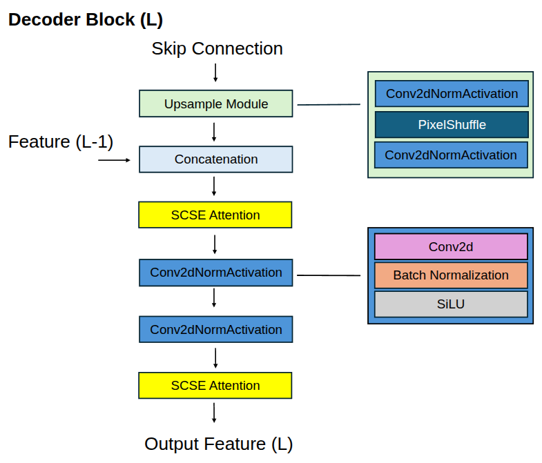
Each decoder is composed of five decoder blocks which progressively upsample the features. Within each block, we incorporate several key components to enhance performance. A detailed illustration of the decoder block design is provided in Figure 3.
-
1.
SCSE Attention: We integrate Spatial and Channel Squeeze-and-Excitation (SCSE) modules Roy et al. (2018) to apply channel-wise and spatial attention, recalibrating and refining the learned feature maps.
-
2.
PixelShuffle Upsampling: To better preserve both spatial and channel fidelity during upsampling, we use PixelShuffle Shi et al. (2016), an operation that rearranges elements from the channel dimension of a low-resolution feature map into spatial dimensions, increasing resolution without interpolation artifacts.
-
3.
SiLU Activation: The SiLU activation function is used throughout the decoder blocks to allow for a smooth gradient flow and stable training.
3.4.3 Multi-Task Learning Framework
To guide each decoder in learning robust morphological representations, we employ a multi-task learning framework. Specifically, in addition to nuclei detection, each decoder is trained using two auxiliary tasks for its specific cell type: nuclei segmentation and nuclei contour segmentation.
-
1.
Nuclei Centroid Detection (primary task): A binary mask of dilated centroids.
-
2.
Nuclei Segmentation (auxiliary task): A binary mask of the full shape of the nuclei.
-
3.
Nuclei contour segmentation (auxiliary task): A binary mask of the nuclei boundaries.
A final sigmoid activation is applied to each of the three outputs, producing probability maps for each task, which are used to compute the loss during training. Figure 4 shows example output masks for nuclei centroid detection, nuclei segmentation, and nuclei contour segmentation.
3.4.4 Architecture Variants for Ablation Studies
To validate the necessity of the independent, multi-decoder design, we introduce two additional KongNet variants for ablation studies:
-
1.
KongNet-SH(Single-Head): This model follows the identical encoder and decoder design as KongNet except that it uses a single, unified decoder which outputs prediction maps for all three tasks and all nuclei types. A diagram of the architecture is shown in Figure S2.
-
2.
KongNet-Det(Detection-only): This lightweight model follows the identical encoder and decoder design as KongNet except that it uses a single decoder to predict only the nuclei centroids for each class (no auxiliary tasks). A diagram of the architecture is shown in Figure S3. We used this lightweight variant for the 2025 MIDOG Challenge, as it allowed for rapid development in a limited time frame without the need to pre-process mitosis annotations into nuclei segmentation or contour masks.
These variations allow us to explore the trade-offs between decoder parameter sharing, model complexity, and performance.

3.5 Loss Functions
To address the multi-class and multi-task nature of the problem, we designed a composite loss function . We begin by defining the overall objective function and then detail its constituent parts.
3.5.1 Overall Objective Function
The overall loss function is the weighted sum of the individual class-specific losses , regularised by a novel inter-class exclusion term, . The equation of the overall loss function is shown in Eq 3.
| (3) |
Where is the loss for the cell class , is its corresponding weight, and is the total number of classes excluding the background class.
This overall objective function has two key components:
-
1.
Cell Class Loss Weighting (): The weights are used for balancing the contributions of different cell classes. We employed two strategies for setting these weights:
-
(a)
Uncertainty-Based Weighting: For the MONKEY and PUMA datasets, we used the method proposed by Kendall et al. Kendall et al. (2017), treating the weights as learnable parameters that are dynamically optimised during training.
-
(b)
Fixed Equal Weighting: For PanNuke and CoNIC datasets, we found that the dynamic approach suppressed the losses from rare classes. Therefore, we used a fixed, equal weighting scheme for all classes, ensuring a sufficient learning signal for under-represented cell types.
-
(a)
-
2.
Inter-class Exclusion Loss (): To encourage mutually exclusive predictions, we introduce a global exclusion loss that penalises simultaneous activations across multiple classes for a given pixel. Unlike pairwise penalties, which can soften class boundaries, our term encourages a winner-takes-all behaviour. It is calculated as the product of the predicted probability maps across all classes. The equation is given in Eq. 4.
(4) where is the total number of pixels, is the total number of cell classes. is the predicted probability that pixel belongs to class .
3.5.2 Class-Specific Loss
represents the total loss for a single specialised decoder responsible for detecting cell type . It is a combination of losses from the three simultaneous prediction tasks: centroid detection , nuclei segmentation , and contour segmentation . We assign a smaller weight (0.5) to the contour loss, as it serves primarily as a guiding signal for the segmentation task. This is shown in Eq. 5.
| (5) |
In the following equations, denotes the binary ground truth for class at pixel , and is the corresponding predicted probability, is the total number of pixels in the image.
-
1.
Segmentation and Contour Loss: For both auxiliary tasks: nuclei segmentation and contour segmentation, we use the same composite loss function , which combines Binary Cross-Entropy () for pixel-level accuracy and Dice loss () for capturing overall shape similarity. This is shown in Eq. 6.
(6) (7) (8) -
2.
Centroid Loss (): For the primary task of nuclei centroid detection, we use a more robust combination of three losses: Jaccard Loss, Dice Loss, and Focal Loss. Dice and Jaccard losses focus on improving overall overlap, while Focal loss places more emphasis on hard-to-detect nuclei where the model often predicts with low confidence. This is shown in Eq. 9
(9) (11) and .
3.6 Evaluation Metrics
To ensure consistency and enable direct comparison with other state-of-the-art methods, we adopted the official evaluation protocols for each dataset and Grand Challenge.
3.6.1 MONKEY Challenge Evaluation
The primary metric for the MONKEY Challenge is the Free Response Operating Characteristic (FROC) analysis. In FROC analysis, the true positive rate (TPR) is plotted against the average number of false positives (FP) per across all slides and across a range of detection confidence thresholds. A predicted detection is considered a true positive (TP) if its centroid lies within a predefined distance margin from a ground truth annotation. For lymphocytes and monocytes, the distance margins are set to and , respectively. For combined inflammatory cell detection, a margin of is used.
Using these definitions, true positives (TP), false positives (FP), and false negatives (FN) are computed for each model to generate the corresponding FROC curve. The final FROC score is calculated as the average sensitivity measured at five pre-specified false positive rates (FP), as defined by the challenge organisers.
It is important to note that inflammatory cells, monocytes, and lymphocytes are evaluated independently. This allows for a soft classification of cells, where a single cell can be assigned to multiple classes with different probabilities.
3.6.2 Evaluation of PanNuke Models
For the PanNuke dataset, we followed the official evaluation protocol, which uses a combined detection and classification F1 score. A prediction is matched to a ground truth nucleus if their centroids are within a 12-pixel radius. The evaluation penalises both detection errors and classification errors within the F1 score calculation.
The overall detection F1 score, precision, and recall (, , ) are calculated as:
| (12) | ||||
| (13) | ||||
| (14) |
Following detection matching, the classification F1 score, precision, and recall per class (, , ) are computed as:
| (15) | ||||
| (16) | ||||
| (17) |
3.6.3 Evaluation for CoNIC, PUMA and MIDOG Models
For CoNIC data, PUMA and MIDOG challenges, detection quality is computed using the F1 score for each cell class, defined as:
| (18) |
where , , and denote the true positive, false positive, and false negative counts for class , respectively.
For CoNIC dataset, the , , and counts are first aggregated across all test images for each cell class before the F1 score is calculated. While the official CoNIC metric is based on segmentation intersection-over-union (IoU), our model is designed to predict centroids. Therefore, consistent with other detection-based methods, we match the predicted and ground truth centroids using a fixed radius of 6 pixels (the standard matching radius for resolution as described in the CellViT paper Hörst et al. (2024)).
The PUMA Challenge also uses the per-class F1 score as its primary metric. However, unlike CoNIC, the F1 score is calculated on a per-image basis for each class, and these scores are then averaged across all images to produce the final result. Predicted and ground truth centroids are matched using a fixed radius of 15 pixels.
The evaluation of the 2025 MIDOG Challenge is similar to CoNIC, where the performance is calculated by aggregating counts across all images before computing the final F1 score. A predicted mitosis is matched to a ground truth annotation if their centroids are within a radius of .
4 Results
For consistency with the original sources, results from prior publications and official challenge leaderboards are reported using the values and decimal precision provided in those sources. Consequently, the number of decimal places is not always uniform across datasets and benchmarks.
4.1 MONKEY Challenge Results
As the model was initially developed for the MONKEY challenge, we first report the performance of the model on our internal cross validation for the MONKEY Challenge. The MONKEY Challenge comprised two tracks: Track 1, ranked by the FROC score for overall inflammatory cell detection, and Track 2, ranked by the average FROC score for lymphocyte and monocyte classification.
4.1.1 Internal Validation Confirms Multi-Decoder Advantage
We first performed a rigorous five-fold cross-validation on the MONKEY training set to optimise our architecture, the results are reported in Table S1. These results clearly established the superiority of our proposed multi-decoder design. The baseline KongNet-Det (detection-only) showed the lowest performance, while KongNet-SH (single-head multi-task) offered improvement. However, the full KongNet, with its independent, class-specific decoders, achieved the best results.
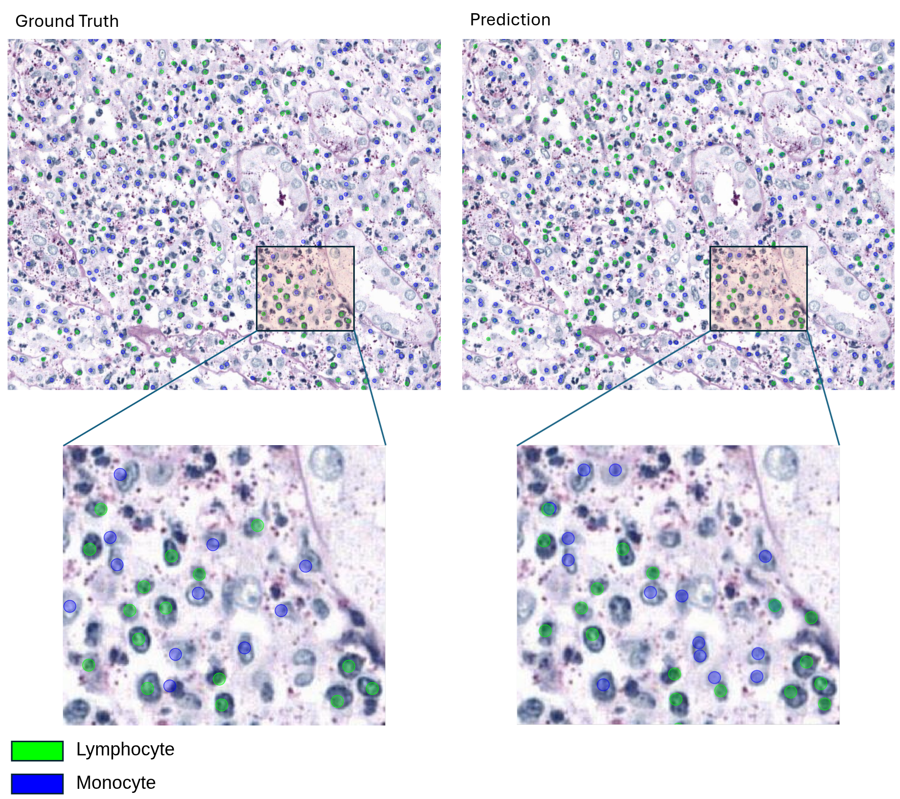
Based on this, we created a final, wider version, KongNet (Wide), by increasing the channel capacity in the decoder blocks to . This configuration demonstrated the highest performance in our internal validation and was selected as our submission for the official challenge. A qualitative example of its predictions is shown in Figure 5.
4.1.2 Preliminary Leaderboard Performance
On the preliminary leaderboard, KongNet (Wide) ranked a strong second overall, achieving competitive FROC scores that were close to the top-performing team and demonstrated a clear advantage over other participants (See Table S2). The preliminary test set consisted of only nine cases from a single unseen medical centre. To avoid overfitting to this small sample, we deliberately refrained from further fine-tuning our model or post-processing parameters based on these results.
4.1.3 Final Leaderboard Performance
On the final leaderboard, KongNet (Wide) secured first place in overall inflammatory cell detection (FROC: 0.3930) and first place in lymphocyte detection (FROC: 0.4624), outperforming all other teams in these categories (Table 2). For the monocyte class, our model ranked second (0.2392), behind Team InstanSeg who leveraged over two million synthetically generated annotations from IHC images Goldsborough . This may have contributed to their superior detection performance for monocytes, an under-represented class in the original dataset.
Our model’s performance on lymphocyte and monocyte detection increased significantly from the preliminary to the final phase, despite the final test set introducing a domain shift with images from two previously unseen medical centres. This demonstrates robustness and generalisation capability of the KongNet architecture compared to other SOTA models such as YOLO, Faster-RCNN, and CellViT. These results validate the effectiveness of using specialised decoders for the highly challenging task of differentiating mononuclear leukocytes in PAS-stained images.
| Method | Inflammatory Cells | Lymphocytes | Monocytes |
|---|---|---|---|
| KongNet (Wide) | 0.3930 | 0.4624 | 0.2392 |
| Team InstanSeg1 | 0.3875 | 0.4515 | 0.2626 |
| Team AIRA Matrix2 | 0.3517 | 0.4471 | 0.1906 |
| Team ST Medical3 | 0.3316 | 0.3935 | 0.1268 |
| Team BioTotem4 | 0.3130 | 0.3702 | 0.1230 |
| Team ouradiology5 | 0.2824 | 0.3703 | 0.1550 |
| Team Zip Lab UNIMORE6 | 0.2470 | 0.3049 | 0.0699 |
| Baseline7 | 0.2282 | 0.3120 | 0.1220 |
4.2 CoNIC Results
To test KongNet’s multi-class classification capabilities on a diverse range of cells, we evaluated it on the challenging CoNIC dataset, which comprises six morphologically diverse cell types: neutrophils, epithelial cells, lymphocytes, plasma cells, eosinophils, and connective tissue cells.
We compare KongNet against the top published submissions from the CoNIC Challenge. The results are shown in Table 3. KongNet achieved a state-of-the-art class-average F1 score of 0.653, outperforming all other published methods, including the winner of the original challenge (StarDist). KongNet secured the highest F1 score in five of the six cell categories, with StarDist showing a small advantage for plasma cells (0.612 vs. 0.596). The qualitative results in Figure 6 further demonstrate KongNet’s robust detection quality across images with significant variations in staining, lighting, and cell morphology.
This SOTA performance was achieved using the same architecture optimised for the PAS-stained MONKEY dataset. This successful transfer from a two-class renal pathology task to a six-class oncology benchmark strongly underscores the inherent generalisability of our specialised multi-decoder approach, highlighting its effectiveness across different tissue types, cell morphologies, and staining protocols.
| Method | Neu | Epi | Lym | Pla | Eos | Con | Class Average |
|---|---|---|---|---|---|---|---|
| KongNet* | 0.510 | 0.818 | 0.707 | 0.596 | 0.591 | 0.695 | 0.653 |
| EPFL (StarDist) Weigert and Schmidt (2022) | 0.476 | 0.762 | 0.696 | 0.612 | 0.497 | 0.653 | 0.616 |
| MDC Berlin Rumberger et al. (2022) | 0.380 | 0.739 | 0.676 | 0.578 | 0.534 | 0.644 | 0.592 |
| Pathology AI Zhang et al. (2024) | 0.415 | 0.741 | 0.693 | 0.562 | 0.445 | 0.627 | 0.581 |
| Arontier Ahn and Hong (2022) | 0.343 | 0.726 | 0.651 | 0.583 | 0.472 | 0.633 | 0.568 |
| AI_Medical Yang et al. (2022) | 0.377 | 0.735 | 0.675 | 0.587 | 0.450 | 0.632 | 0.513 |

4.3 PanNuke Results
We tested KongNet on the PanNuke dataset, a highly diverse benchmark featuring 19 tissue types. Using the official evaluation protocol, we report the average F1 scores in Table 4.
KongNet achieved the highest class-average F1 score (0.674), demonstrating a more balanced performance profile than other leading methods. Specifically, our model excelled in classifying cell types often identified by their distinct individual morphology: inflammatory (0.72), connective (0.70), and dead cells (0.59). In contrast, the transformer-based CellNuc-DETR performed best on neoplastic and epithelial cells, categories where broader tissue context may play a larger role. This suggests a complementary strength of our CNN-based, multi-decoder approach in capturing fine-grained local features.
Compared to other established methods such as STARDIST and HoVer-Net, KongNet shows a clear advantage in both overall and per-class performance. The strong results underscore the effectiveness of our architecture, which significantly outperforms transformer-based models such as CellViT that do not leverage massive pre-training, confirming the importance of task-specific architectural design. The qualitative results in Figure 7 further illustrate KongNet’s strong and balanced detection quality.
| Method | Overall | Neo | Inf | Epi | Con | Dead | Class Average |
|---|---|---|---|---|---|---|---|
| KongNet | 0.84 | 0.71 | 0.72 | 0.65 | 0.70 | 0.59 | 0.674 |
| CellNuc-DETR Pina et al. (2025) | 0.84 | 0.72 | 0.60 | 0.74 | 0.56 | 0.45 | 0.618 |
| NuLite-H Tommasino et al. (2024) | 0.83 | 0.71 | 0.58 | 0.73 | 0.53 | 0.37 | 0.584 |
| CellViT-SAM-H Hörst et al. (2024) | 0.83 | 0.71 | 0.58 | 0.73 | 0.53 | 0.36 | 0.582 |
| HoVer-NeXt Baumann et al. (2024) | 0.76 | 0.61 | 0.66 | 0.55 | 0.56 | 0.53 | 0.582 |
| DualU-Net Anglada-Rotger et al. (2025b) | 0.80 | 0.66 | 0.58 | 0.61 | 0.52 | 0.36 | 0.548 |
| CellViT no pre-train Hörst et al. (2024) | 0.80 | 0.64 | 0.55 | 0.72 | 0.48 | 0.31 | 0.540 |
| STARDIST Weigert and Schmidt (2022) | 0.82 | 0.69 | 0.57 | 0.70 | 0.51 | 0.10 | 0.514 |
| HoVer-Net Graham et al. (2019) | 0.80 | 0.62 | 0.54 | 0.56 | 0.49 | 0.31 | 0.504 |

4.4 PUMA Challenge Results
We further tested KongNet’s adaptability in the 2025 PUMA Challenge, which involved detecting and classifying nuclei in H&E-stained images of advanced melanoma. The challenge featured two tracks of increasing complexity.
4.4.1 PUMA Track 1: 3-Class Detection
Track 1 focused on detecting three broad categories: tumour, lymphocytes, and other cells. In the preliminary leaderboard, KongNet ranked first across all cell types, achieving F1 scores of 0.8103 for tumour cells, 0.8070 for lymphocytes, and 0.5006 for other cells. The results are shown in Table S9.
On the final leaderboard (Table 5), KongNet remained highly competitive. With a macro-average F1 of 0.6466, our model placed third overall in a very competitive race. KongNet achieved the highest F1 score (0.6746) for lymphocyte detection among all submitted methods. The primary reason for this outcome was that we only fine-tuned KongNet on the PUMA dataset within a limited time frame, using weights previously trained on the MONKEY model for lymphocyte and monocyte detection. Furthermore, KongNet significantly outperformed both the official HoVer-NeXt baseline and a fine-tuned CellViT++ model, demonstrating its robust performance against other SOTA approaches.
| Method | Average | Tumour | Lymphocytes | Other |
|---|---|---|---|---|
| Team rictoo* | 0.6585 | 0.8210 | 0.6729 | 0.4818 |
| Team LSM1 | 0.6501 | 0.7991 | 0.6537 | 0.4977 |
| KongNet | 0.6466 | 0.7948 | 0.6746 | 0.4704 |
| Baseline2 | 0.5979 | 0.7282 | 0.6611 | 0.4046 |
| Team UME3 | 0.5863 | 0.7614 | 0.6278 | 0.3697 |
4.4.2 PUMA Track 2
Track 2 substantially increased the difficulty, requiring classification of ten distinct cell types. Again, KongNet ranked first overall in the preliminary phase. The results are shown in Table S10.
In the final test phase, KongNet secured a close second place overall with a macro-average F1 score of 0.2656, narrowly behind the winning team (0.2707), but much superior to other methods such as HoVer-NeXt and CellViT++ as shown in Table 6. The performance of our model was comparable to or exceeded the leading teams in most categories. KongNet again achieved the highest score for lymphocyte detection (0.6642) and also excelled at detecting melanophages and plasma cells compared to other methods. The performance gap to the winner (Team LSM) was primarily in rare or ambiguous classes like apoptotic cells, where their multi-stage pipeline, which incorporates tissue-level context, likely provided an advantage. This highlights a potential avenue for future improvement by integrating contextual information.
A qualitative review of our model’s failure cases (Figure 8) confirms these findings. The model occasionally confused apoptotic cells with lymphocytes and struggled to differentiate between tumour and epithelial cells, particularly in the absence of broader tissue context. This is likely because apoptotic cells often exhibit fragmented nuclei, which can resemble the small and rounded nuclei of lymphocytes. Another contributing factor may be the limited number of training examples containing necrotic regions. We also observed that distinguishing between tumour and epithelial cells can be challenging (Figure 8.b), as both share similar morphological features. These results indicate the potential value of incorporating tissue-type context into cell classification. For example, necrotic regions are more likely to contain apoptotic cells, while epidermal regions predominantly consist of epithelial cells rather than tumour cells.

| Method | Average | Tum | Str | Apo | Epi | His |
|---|---|---|---|---|---|---|
| Team LSM1 | 0.2707 | 0.7935 | 0.2978 | 0.1641 | 0.0817 | 0.2401 |
| KongNet | 0.2656 | 0.7952 | 0.2927 | 0.1170 | 0.0707 | 0.2154 |
| Team rictoo* | 0.2416 | 0.8190 | 0.2319 | 0.0394 | 0.0809 | 0.2413 |
| Team UME3 | 0.2335 | 0.7574 | 0.2500 | 0.1116 | 0.0632 | 0.2064 |
| Baseline2 | 0.2040 | 0.6795 | 0.1980 | 0.0262 | 0.0056 | 0.1885 |
| Method | Lym | Neu | End | Mel | Pla |
|---|---|---|---|---|---|
| Team LSM1 | 0.6299 | 0.0688 | 0.2053 | 0.1795 | 0.0465 |
| KongNet | 0.6642 | 0.0361 | 0.2123 | 0.1931 | 0.0595 |
| Team rictoo* | 0.6136 | 0.0068 | 0.2359 | 0.1474 | 0.0 |
| Team UME3 | 0.6107 | 0.0220 | 0.1421 | 0.1494 | 0.0218 |
| Baseline2 | 0.5847 | 0.0402 | 0.1553 | 0.1200 | 0.0422 |
4.5 MIDOG Challenge 2025 Results
To validate the effectiveness and efficiency of our architectural principles on a completely different task, we employed our lightweight variant KongNet-Det, for mitosis detection during the MIDOG 2025 Challenge. This evaluation served as a rigorous benchmark of KongNet-Det in a highly competitive and challenging environment.
4.5.1 Preliminary Leaderboard
As shown in Table S6, in the preliminary phase, KongNet-Det immediately established itself as a top contender, ranking first with an F1 score of 0.8147. Notably, our model achieved a good balance between precision (0.7995) and recall (0.8306) compared to other leading methods, which often skewed towards one or the other.
4.5.2 MIDOG Final Leaderboard
Table 7 shows the performance on the final leaderboard. KongNet-Det once again secured first place with an F1 score of 0.7400. This is particularly significant given the difficulty of the official test set, which was designed to test the robustness of the models by including 12 different tumour types and highly challenging regions of interest (ROIs).
Achieving the top-rank in such a demanding benchmark underscores the power and efficiency of our lightweight architecture, which forms the core component of KongNet. It shows that the core design principles of KongNet are not limited to inflammatory cell detection and classification, but are versatile and can be extended to excel in other cell detection tasks such as mitosis detection.
| Method | F1 | Precision | Recall |
|---|---|---|---|
| KongNet-Det | 0.7400 | 0.7775 | 0.7059 |
| Team CBIO1 | 0.7216 | 0.7731 | 0.6765 |
| Team YTUVisionRG2 | 0.7085 | 0.6961 | 0.7215 |
| Team cacfek3 | 0.7063 | 0.7028 | 0.7098 |
| Team Gestalt4 | 0.7003 | 0.7973 | 0.6244 |
4.6 Ablation Studies
We conducted a series of ablation studies on both the MONKEY and PanNuke datasets to validate two key design choices: the use of a multi-headed, specialised decoder architecture and the inclusion of SCSE attention modules.
4.6.1 Impact of the Multi-Decoder Architecture
First, we evaluated the performance of our main multi-decoder model (KongNet) against its simpler, single-decoder variants (KongNet-SH and KongNet-Det).
The results consistently demonstrate the advantage of using specialised decoders for complex classification tasks. On the MONKEY dataset, the full KongNet significantly outperformed both single-decoder models across all metrics (Table 8). This trend was confirmed on the more complex PanNuke dataset (Table 9). While the single-head variant (KongNet-SH) achieved the same high overall detection F1 score (0.84), the multi-headed KongNet achieved the highest class-average F1 score (0.674). This indicates that although a single decoder is highly effective for general nuclei detection, the specialised decoders are beneficial for the complex task of accurately distinguishing between multiple cell types.
4.6.2 Impact of SCSE Attention Modules
Next, we assessed the benefit of integrating SCSE attention modules within the decoders. The findings confirm their positive impact on performance. For our main KongNet architecture, adding SCSE modules consistently improved performance on the MONKEY dataset, for example, raising the FROC score of monocytes from 0.2170 to 0.2407 (Table 8). On the PanNuke dataset, for example, adding SCSE modules to KongNet increased the class-average F1 score from 0.656 to 0.674 (Table 9). While the improvements were less pronounced for the single-decoder variants, the consistent gains observed for our primary KongNet architecture confirmed their importance. Based on these findings, SCSE modules were integrated into our final model configuration, contributing to its strong and robust performance.
| Method | Inflammatory Cells | Lymphocytes | Monocytes |
|---|---|---|---|
| KongNet-Det No SCSE | |||
| KongNet-Det | |||
| KongNet-SH No SCSE | |||
| KongNet-SH | |||
| KongNet No SCSE | |||
| KongNet |
| Method | Overall | Neo | Inf | Epi | Con | Dead | Class Average* |
|---|---|---|---|---|---|---|---|
| KongNet-Det No SCSE | 0.83 | 0.69 | 0.71 | 0.63 | 0.67 | 0.58 | 0.656 |
| KongNet-Det | 0.83 | 0.69 | 0.72 | 0.61 | 0.66 | 0.58 | 0.652 |
| KongNet-SH No SCSE | 0.84 | 0.71 | 0.73 | 0.63 | 0.70 | 0.60 | 0.674 |
| KongNet-SH | 0.84 | 0.71 | 0.72 | 0.63 | 0.70 | 0.60 | 0.672 |
| KongNet No SCSE | 0.84 | 0.70 | 0.71 | 0.60 | 0.69 | 0.58 | 0.656 |
| KongNet | 0.84 | 0.71 | 0.72 | 0.65 | 0.70 | 0.59 | 0.674 |
5 Inference Speed and Efficiency
5.1 Whole-Slide Image Inference Runtime
To assess practical deployment efficiency, we benchmarked the end-to-end inference time for a full whole-slide image (WSI). The benchmark was performed at magnification using a TCGA slide (ID:TCGA-AN-A0XP-01Z-00-DX1), which contains approximately of foreground tissue. We compared KongNet against HoVer-NeXt Tiny and CellViT-SAM-H on two hardware tiers: a standard workstation and a high-performance computing (HPC) node, reflecting different resource environments in pathology labs.
Hardware specifications:
-
1.
Workstation: NVIDIA RTX 3060 (12 GB), Intel Core i5-13500 (14 cores), 32 GB RAM
-
2.
HPC Node: NVIDIA V100 (32 GB), Intel Xeon Platinum 8168 (32 cores), 80 GB RAM
The CellViT inference pipeline automatically selects batch size and the number of worker threads based on available hardware. HoVer-NeXt Tiny was configured with pp_tiling=16, inf_workers=10, and pp_workers=10 on the workstation, and with inf_workers=32 and pp_workers=32 on the HPC node.
On the workstation (Table S12), KongNet demonstrated excellent efficiency. Without test-time augmentation (TTA), it processed the WSI in just 8 minutes. Using 4× TTA, which offers the best balance of accuracy and speed, the runtime was 26 minutes, TTA increases the runtime to 94 minutes. HoVer-NeXt Tiny ( TTA) completes inference in 31 minutes, we used TTA as this setting achieves the reported detection performance. The 699-million-parameter CellViT-SAM-H failed to run on the workstation due to memory errors, highlighting the hardware barrier large transformer models present for deployment in typical, resource-constrained settings.
On the HPC node (Table S13), KongNet requires only 6 minutes without TTA, 14 minutes with TTA, and 43 minutes with TTA. CellViT-SAM-H was successfully evaluated on the HPC node, requiring 18 minutes total, longer than KongNet with no TTA.
In summary, although in our main results section we report the performance of KongNet with TTA, running KongNet with TTA could offer the best trade-off between detection quality and computational efficiency, which is a more practical choice for real-world applications. We found that TTA yields minimal accuracy gains over TTA on PanNuke dataset (Table S11)
5.2 Isolated Model Forward Pass Latency
To measure raw model speed independent of the processing pipeline, we benchmarked the average forward pass time on the workstation hardware. As expected, the much smaller HoVer-NeXt Tiny was the fastest, with a latency of just 0.0133 seconds. KongNet’s forward pass (0.0378 s) was approximately four times faster than CellViT-SAM-H (0.1510 s) and slightly faster than the smaller CellViT 256 (0.0384 s) despite having 3.8 times more parameters. This suggests that the architectural design of KongNet, being a convolutional neural network (CNN), benefits from hardware-level optimisations compared to certain operations in Vision Transformers (ViTs) such as self-attention and LayerNorm, which can be computationally intensive. The results are summarised in Table S14.
6 Discussion
6.1 CNNs vs ViT
Our results highlight the distinct, complementary strengths of Convolutional Neural Networks (CNNs) and Vision Transformers (ViTs) for nuclei detection and classification. ViTs excel at modelling long-range spatial dependencies through self-attention, making them adept at integrating tissue context. In contrast, CNNs remain unparalleled at learning the fine-grained local morphological features that are often the primary discriminative information in histopathology. To further investigate this point within our own framework, we compared CNN- and transformer-based encoder backbones for KongNet on the MONKEY dataset. As shown in Table S3 of the Supplementary Material, the CNN-based EfficientNetV2-L encoder achieved the strongest overall performance.
This dichotomy is evident in the PanNuke results (Table 4). Our CNN-based KongNet excelled at classifying cell types defined by their distinct nuclear morphology, such as inflammatory, connective, and dead cells. ViT-based models such as CellViT and CellNuc-DETR showed an advantage in classifying neoplastic and epithelial nuclei categories, where the surrounding tissue architecture provides a crucial context to which ViTs are better suited. The MONKEY Challenge results (Table 2) further support this: in a task where subtle morphological differences between lymphocytes and monocytes are key and broader context is less informative, CNN-based models, including ours, outperformed ViT-based approaches.
These findings suggest a task-dependent synergy. CNN-based architectures such as KongNet appear optimal when classification is based on the morphology of the nucleus itself, while ViTs may hold an advantage when the task relies on interpreting broader spatial context. This points toward a promising future direction: hybrid architectures that skilfully combine the local feature extraction power of CNNs with the global context modelling of ViTs.
6.2 Impact of the Multi-headed Architecture
To better understand why the relative performance of the single-head and multi-head variants differs across datasets, we investigated whether this behaviour is driven by the intrinsic characteristics of the datasets. Overall, our results suggest that the dominant factor is the dataset characteristics, in particular the degree of morphological separability between cell classes.
On the MONKEY dataset, the multi-head architecture provides a clear advantage over the single-head variant across all three cell categories. KongNet-SH achieved FROC scores of 0.3263, 0.3902, and 0.2208 for inflammatory cells, lymphocytes, and monocytes, respectively, whereas the multi-head KongNet improved these to 0.3537, 0.3950, and 0.2407 (Table S1). In contrast, on the PanNuke dataset, KongNet and KongNet-SH achieved very similar overall performance, with class-average F1 scores of 0.674 and 0.672, respectively (Table 9). These findings indicate that the benefit of class-specific decoders is dependent on the difficulty of the underlaying cell classification problem.
We hypothesised that the tasks requiring separation of highly overlapping cell morphologies benefit more from a multi-headed architecture, whereas tasks in which the target cell classes are more readily separable gain smaller benefit from decoder specialisation. In particular, the MONKEY dataset requires separating lymphocytes and monocytes, which exhibit highly similar morphology, while the PanNuke dataset contains several classes that are more readily distinguishable. To test this hypothesis, we analysed nuclei distributions in feature space for both datasets. For each dataset, we first extracted nuclei instances from the available segmentation masks (Examples are shown in Figure S4). For MONKEY, we used NuClick generated masks employed during KongNet training, for PanNuke we used the provided instance annotations. Then, for each nucleus, we computed a set of hand-crafted shape descriptors (Supplementary Material A.5.6) and extracted deep features using an ImageNet pretrained ResNet18 model. We then treated each cell type as a cluster in feature space and quantified cluster separability using the Davies–Bouldin (DB) index Davies and Bouldin (1979), where lower values indicate more compact and better separated clusters.
In the MONKEY dataset, the two target classes, lymphocytes and monocytes, showed relatively poor separability, with DB indices of 6.74 in the shape-feature space and 7.57 in the ResNet18 feature space (Table S15). By contrast, in PanNuke, most pairwise class comparisons yielded substantially lower DB values, indicating better class separation overall. The only exception was the pair neoplastic versus epithelial cells, which exhibited the highest overlap in PanNuke, with DB indices of 11.61 and 8.32 for shape and ResNet18 features respectively (Table S16). This is consistent with the observation that the multi-head design provides only a modest overall gain on PanNuke, with the most benefit arising in the detection of neoplastic and epithelial cells, thus supporting our hypothesis.
Figure S5 provides a qualitative visualisation of clusters. In the MONKEY dataset, the lymphocyte and monocyte clusters show substantial overlap, consistent with their relatively high DB indices. In the PanNuke dataset, the neoplastic and epithelial classes also appear less well separated than other pairs such as dead and neoplastic classes, which visually reflects the corresponding DB values. Although t-SNE is only a qualitative projection, it provides an intuitive illustration of the same trend captured quantitatively by the DB index.
To further examine the role of loss weighting, we evaluated automatic class-wise loss weighting on the PanNuke dataset using the same strategy employed for MONKEY. As shown in Table S17, automatic weighting reduced the class-average F1 score of KongNet from 0.674 to 0.654, indicating that it is inferior to the fixed equal-weighting scheme. We therefore used equal values for PanNuke in all main comparisons, as this provided the strongest performance for the model. Consequently, the comparison between KongNet-SH and KongNet-MH on PanNuke was already performed under the optimal loss-weighting setting we identified, indicating that the small difference between the two variants is unlikely to be explained by the choice of values.
Together, these findings suggest that the effectiveness of the multi-headed design depends on the task and the structure of the dataset. When the target classes are morphologically similar and occupy strongly overlapping regions of feature space, as in the MONKEY dataset, independent decoder heads appear to provide an improved class separation. When the classes are already relatively well separated, as for most the PanNuke dataset categories, the advantage of the multi-headed design is smaller.
6.3 Tissue-Guided Cell Classification
Previous work, such as OCELOT Ryu et al. (2023), has shown that incorporating tissue-level context can enhance cell classification accuracy, particularly in complex tumour microenvironment. However, the OCELOT dataset was limited to only two types of classifications, tumour vs non-tumour cells and tissue.
The PUMA Challenge results underscore the important role of tissue context in resolving cellular ambiguity. The winning team (Team LSM Torbati et al. (2025)) employed a multi-stage pipeline that used tissue segmentation maps to guide and refine nuclei classification, allowing them to outperform our model. Their advantage was most pronounced for apoptotic cells, a morphologically ambiguous category. As shown in our qualitative analysis and supported by their results (Table 6), apoptotic cells frequently occur within necrotic tissue regions. A model aware of this necrotic context is more likely to correctly classify ambiguous nuclear fragments as apoptotic, whereas a context-agnostic model like ours may confuse them with immune cells such as lymphocytes.
This strongly suggests that the next major advance in cell classification, particularly for ambiguous or transitional cell states, lies in joint tissue-cell modelling. While KongNet in its current form does not leverage this information, a clear and promising path for future work is to integrate tissue context directly into the architecture. This could allow the model to make more informed, pathologist-like decisions in challenging histopathological settings.
7 Conclusion
In this work, we introduced KongNet, a multi-headed deep learning architecture designed for accurate and generalisable cell detection and classification in histopathology. The model’s core contribution is its use of parallel, cell-type-specialised decoders, enhanced by SCSE attention and a multi-task learning framework that jointly predicts centroids, segmentation masks, and contours. This design proved highly effective at learning discriminative morphological features while minimising inter-class interference.
We demonstrated the power and robustness of this approach through a comprehensive evaluation across multiple Grand Challenges and public benchmarks. KongNet and its lightweight variant, KongNet-Det, achieved first-place victories in the MONKEY Challenge for inflammatory cell detection and the 2025 MIDOG Challenge for mitosis detection, respectively. Moreover, KongNet also secured top-three rankings in the highly complex PUMA Challenge and established new state-of-the-art performance on the PanNuke and CoNIC datasets, proven its effectiveness across diverse tissues, cell types, and staining protocols.
In summary, KongNet provides a robust, adaptable, and highly competitive architectural foundation for a wide range of nuclei analysis tasks. Its consistent state-of-the-art performance establishes it as a powerful and practical tool for the computational pathology community.
Future work will focus on leveraging this tool for large-scale analysis of the tumour microenvironment (TME). We plan to create a comprehensive pipeline by combining KongNet with our first-place-winning tissue segmentation model Lv et al. (2026) from the PUMA Challenge. Furthermore, inspired by our findings in the Discussion, we will explore next-generation architectures incorporating contextual information that explicitly integrates tissue context to further enhance classification accuracy in the most challenging histopathological settings.
Code Availability
-
1.
Full inference code can be accessed on GitHub at this link https://github.com/Jiaqi-Lv/KongNet_Inference_Main.
-
2.
The model is also accessible as a Jupyter Notebook in TIAToolBox Pocock et al. (2022), which can be accessed at this link https://tia-toolbox.readthedocs.io/en/latest/_notebooks/jnb/12-nucleus-detection.html.
Acknowledgement
JL is supported by the UK Engineering and Physical Sciences Research Council (EPSRC). SEAR reports financial support by the MRC (MR/X011585/1) and the BigPicture project, which has received funding from the Innovative Medicines Initiative 2 Joint Undertaking under grant agreement No 945358. We thank the organisers and contributors of the MONKEY Challenge, the CoNIC Challenge, the PUMA Challenge, and the 2025 MIDOG challenge, for providing the valuable datasets and evaluation platforms.
References
- Class-controlled copy-paste based cell segmentation for conic challenge. bioRxiv. External Links: Document, Link, https://www.biorxiv.org/content/early/2022/03/04/2022.03.02.482203.full.pdf Cited by: Table 3.
- NuClick: a deep learning framework for interactive segmentation of microscopic images. Medical Image Analysis 65, pp. 101771. External Links: ISSN 1361-8415, Document, Link Cited by: §3.2.
- Mitosis domain generalization challenge 2025. Zenodo. External Links: Document, Link Cited by: §1.
- Two heads are enough: dualu-net, a fast and efficient architecture for nuclei instance segmentation. In Medical Imaging with Deep Learning, External Links: Link Cited by: §2.
- Two heads are enough: dualu-net, a fast and efficient architecture for nuclei instance segmentation. In Medical Imaging with Deep Learning, External Links: Link Cited by: Table 4.
- A completely annotated whole slide image dataset of canine breast cancer to aid human breast cancer research. Scientific Data 7 (1), pp. 417 (en). External Links: ISSN 2052-4463, Link, Document Cited by: §3.1.5, Table 1.
- A comprehensive multi-domain dataset for mitotic figure detection. Scientific Data 10 (1), pp. 484 (en). External Links: ISSN 2052-4463, Link, Document Cited by: §3.1.5, Table 1.
- HoVer-next: a fast nuclei segmentation and classification pipeline for next generation histopathology. In Medical Imaging with Deep Learning, External Links: Link Cited by: §2, Table 4.
- A large-scale dataset for mitotic figure assessment on whole slide images of canine cutaneous mast cell tumor. Scientific Data 6 (1), pp. 274. External Links: ISSN 2052-4463, Document, Link Cited by: §3.1.5, Table 1.
- Robust pan-cancer mitotic figure detection with yolov12. External Links: 2509.02593, Link Cited by: Table S6, Table S6, Table 7, Table 7.
- Tumour-infiltrating lymphocytes: from prognosis to treatment selection. British Journal of Cancer 128 (3), pp. 451–458. External Links: ISSN 1532-1827, Document, Link Cited by: §1.
- Albumentations: fast and flexible image augmentations. Information 11 (2). External Links: Link, ISSN 2078-2489, Document Cited by: §A.5.
- [13] AImageLab-zip-monkey-challenge-ziplab: aimagelab zip unimore solution for the monkey challenge of radboud university medical center. External Links: Link Cited by: Table 2, Table 2.
- [14] Lynn0304-monkey-challenge. External Links: Link Cited by: Table 2, Table 2.
- A cluster separation measure. IEEE Transactions on Pattern Analysis and Machine Intelligence PAMI-1 (2), pp. 224–227. External Links: Document Cited by: §6.2.
- The evolving tumor microenvironment: from cancer initiation to metastatic outgrowth. Cancer Cell 41 (3), pp. 374–403. External Links: ISSN 1535-6108, Document, Link Cited by: §1.
- Advancements in automated nuclei segmentation for histopathology using you only look once-driven approaches: A systematic review. Computers in Biology and Medicine 190, pp. 110072. External Links: ISSN 0010-4825, Document Cited by: §2.
- Ensemble object detection methodology for automated detection of inflammatory cells in kidney biopsies. In Medical Imaging with Deep Learning - Short Papers, External Links: Link Cited by: Table 2, Table 2.
- The tale of TILs in breast cancer: a report from the international Immuno-Oncology biomarker working group. NPJ Breast Cancer 7 (1), pp. 150 (en). Cited by: §1.
- PanNuke dataset extension, insights and baselines. External Links: 2003.10778, Link Cited by: item 5, §1, §3.1.3, §3.1, Table 1.
- InstanSeg: an embedding-based instance segmentation algorithm optimized for accurate, efficient and portable cell segmentation. External Links: 2408.15954, Link Cited by: §2.
- [22] Thibautgoldsborough-instanseg-monkey-challenge. External Links: Link Cited by: §4.1.3, Table 2, Table 2.
- CoNIC challenge: pushing the frontiers of nuclear detection, segmentation, classification and counting. Medical Image Analysis 92, pp. 103047. External Links: ISSN 1361-8415, Document, Link Cited by: item 5, §1, §2, §3.1.2, §3.1, Table 1.
- Hover-net: simultaneous segmentation and classification of nuclei in multi-tissue histology images. Medical Image Analysis 58, pp. 101563. External Links: ISSN 1361-8415, Document, Link Cited by: §2, Table 4.
- TransNuSeg: a lightweight multi-task transformer for nuclei segmentation. In Medical Image Computing and Computer Assisted Intervention – MICCAI 2023, H. Greenspan, A. Madabhushi, P. Mousavi, S. Salcudean, J. Duncan, T. Syeda-Mahmood, and R. Taylor (Eds.), Cham, pp. 206–215. External Links: ISBN 978-3-031-43901-8 Cited by: §2.
- CellViT: vision transformers for precise cell segmentation and classification. Medical Image Analysis 94, pp. 103143. External Links: ISSN 1361-8415, Document, Link Cited by: §2, §3.6.3, Table 4, Table 4.
- NnU-net: a self-configuring method for deep learning-based biomedical image segmentation. Nature Methods 18 (2), pp. 203–211. External Links: ISSN 1548-7105, Document, Link Cited by: §2.
- Mitosis subtyping dataset. Zenodo. Note: https://doi.org/10.5281/zenodo.15390543[Data set] Cited by: §3.1.5, Table 1.
- Multi-task learning using uncertainty to weigh losses for scene geometry and semantics. 2018 IEEE/CVF Conference on Computer Vision and Pattern Recognition, pp. 7482–7491. External Links: Link Cited by: item 1a.
- Deep learning for multiclass tumor cell detection in histopathology slides of hereditary diffuse gastric cancer. iScience 28 (8). External Links: ISSN 2589-0042, Document, Link Cited by: §2.
- Leveraging pathology foundation models for panoptic segmentation of melanoma in h&e images. In Medical Image Understanding and Analysis, S. Ali, D. C. Hogg, and M. Peckham (Eds.), Cham, pp. 58–72. External Links: ISBN 978-3-031-98688-8 Cited by: §7.
- A bag of tricks for real-time mitotic figure detection. External Links: 2508.19804, Link Cited by: Table S6, Table S6, Table 7, Table 7.
- The tumor microenvironment shows a hierarchy of cell-cell interactions dominated by fibroblasts. Nature Communications 14 (1), pp. 5810. External Links: ISSN 2041-1723, Document, Link Cited by: §1.
- Cell nuclei detection and classification in whole slide images with transformers. External Links: 2502.06307, Link Cited by: §2, Table 4.
- TIAToolbox as an end-to-end library for advanced tissue image analytics. Communications Medicine 2 (1), pp. 120. External Links: Document, ISSN 2730-664X, Link Cited by: §3.2, item 2.
- Augment like there’s no tomorrow: consistently performing neural networks for medical imaging. External Links: 2206.15274, Link Cited by: §A.5.
- Deconvolving convolutional neural network for cell detection. In 2019 IEEE 16th International Symposium on Biomedical Imaging (ISBI 2019), Vol. , pp. 891–894. External Links: Document Cited by: §2.
- You only look once: unified, real-time object detection. In 2016 IEEE Conference on Computer Vision and Pattern Recognition (CVPR), Vol. , pp. 779–788. External Links: Document Cited by: §2.
- Faster r-cnn: towards real-time object detection with region proposal networks. In Advances in Neural Information Processing Systems, C. Cortes, N. Lawrence, D. Lee, M. Sugiyama, and R. Garnett (Eds.), Vol. 28, pp. . External Links: Link Cited by: §2.
- A 2018 Reference Guide to the Banff Classification of Renal Allograft Pathology. Transplantation 102 (11), pp. 1795–1814. External Links: ISSN 0041-1337, Document Cited by: §1.
- Concurrent spatial and channel squeeze & excitation in fully convolutional networks. External Links: 1803.02579, Link Cited by: item 1.
- Panoptic segmentation with highly imbalanced semantic labels. In 2022 IEEE International Symposium on Biomedical Imaging Challenges (ISBIC), Vol. , pp. 1–4. External Links: Document Cited by: §3.3, Table 3.
- OCELOT: overlapped cell on tissue dataset for histopathology. In Proceedings of the IEEE/CVF Conference on Computer Vision and Pattern Recognition (CVPR), Cited by: §2, §6.3.
- Spatial organization and molecular correlation of tumor-infiltrating lymphocytes using deep learning on pathology images. Cell Reports 23 (1), pp. 181–193.e7. External Links: ISSN 2211-1247, Document, Link Cited by: §1.
- [45] Jun-sato-monkey-challenge-ouradiology: ouradiology approach in monkey challenge. External Links: Link Cited by: Table 2, Table 2.
- A novel dataset for nuclei and tissue segmentation in melanoma with baseline nuclei segmentation and tissue segmentation benchmarks. GigaScience 14, pp. . External Links: Document Cited by: Table S10, Table S10, Table S9, Table S9, item 3, §1, §2, §3.1.4, §3.1, Table 1, Table 1, Table 5, Table 5, Table 6, Table 6.
- Cracking the puma challenge in 24 hours with cellvit++ and nnu-net. External Links: 2503.12269, Link Cited by: Table S10, Table S10, Table S9, Table S9, Table 5, Table 5, Table 6, Table 6.
- Pan-cancer mitotic figures detection and domain generalization: midog 2025 challenge. External Links: 2509.02585, Link Cited by: Table S6, Table S6, Table 7, Table 7.
- Real-time single image and video super-resolution using an efficient sub-pixel convolutional neural network. In 2016 IEEE Conference on Computer Vision and Pattern Recognition (CVPR), Vol. , pp. 1874–1883. External Links: Document Cited by: item 2.
- Locality sensitive deep learning for detection and classification of nuclei in routine colon cancer histology images. IEEE Transactions on Medical Imaging 35 (5), pp. 1196–1206. External Links: Document Cited by: §2.
- Structured description of the monkey challenge. Zenodo. External Links: Document, Link Cited by: Table S2, Table S2, item 3, §1, §3.1.1, §3.1, Table 1, Table 2, Table 2.
- Multi-class cell detection using modified self-attention. In 2022 IEEE/CVF Conference on Computer Vision and Pattern Recognition Workshops (CVPRW), Vol. , pp. 1854–1862. External Links: Document Cited by: §2.
- Size-dependent positioning of human chromosomes in interphase nuclei. Biophysical Journal 79 (1), pp. 184–190. External Links: ISSN 0006-3495, Document, Link Cited by: §3.2.
- EfficientNetV2: smaller models and faster training. External Links: Document Cited by: item 1.
- NuLite – lightweight and fast model for nuclei instance segmentation and classification. External Links: 2408.01797, Link Cited by: §2, Table 4.
- A single detect focused yolo framework for robust mitotic figure detection. External Links: 2509.02637, Link Cited by: Table S6, Table S6, Table 7, Table 7.
- A multi-stage auto-context deep learning framework for tissue and nuclei segmentation and classification in h&e-stained histological images of advanced melanoma. External Links: 2503.23958, Link Cited by: Table S10, Table S10, Table S9, Table S9, §2, Table 5, Table 5, Table 6, Table 6, §6.3.
- Tumor infiltrating lymphocytes across breast cancer subtypes: current issues for biomarker assessment. Cancers (Basel) 15 (3), pp. 767 (en). Cited by: §1.
- Role of tumor microenvironment in cancer progression and therapeutic strategy. Cancer Medicine 12 (10), pp. 11149–11165. External Links: Document, Link, https://onlinelibrary.wiley.com/doi/pdf/10.1002/cam4.5698 Cited by: §1.
- Nuclei instance segmentation and classification in histopathology images with stardist. In 2022 IEEE International Symposium on Biomedical Imaging Challenges (ISBIC), Vol. , pp. 1–4. External Links: Document Cited by: §2, Table 3, Table 4.
- [61] Biototem-monkey-challenge: scripts for monkey challenge 2024. External Links: Link Cited by: Table 2, Table 2.
- A deep learning framework for nuclear segmentation and classification in histopathological images. External Links: 2203.03420, Link Cited by: Table 3.
- Keep it accurate and robust: an enhanced nuclei analysis framework. Comput. Struct. Biotechnol. J. 24, pp. 699–710 (en). Cited by: Table 3.
Supplementary Material
Appendix A Supplementary Information
A.1 Summary of MONKEY Challenge Submission
We used MONKEY Dataset as the primary dataset to iteratively develop our model based on internal cross-validation. We configure KongNet with three decoders, one for overall inflammatory cell detection, one for lymphocytes detection, and one for monocytes detection.
A.2 Summary of PUMA Challenge Submission
We evaluated the adaptability of our model through participation in the PUMA Challenge, which comprised two tracks focusing on nuclei detection and classification in advanced melanoma: Track 1: Detection of three types of cells: tumour cells, tumour-infiltrating lymphocytes (TILs; including lymphocytes and plasma cells), and other cells. Track 2: Detection of ten types of cells: tumour cells, lymphocytes, plasma cells, histiocytes, melanophages, neutrophils, stromal cells, epithelium cells, endothelium cells, and apoptotic cells.
Adapting our model to the PUMA Challenge required only a single modification: adjusting the number of decoders. We used three decoders for Track 1 and ten decoders for Track 2. Due to time constraints, we did not perform hyperparameter tuning.
A.3 Summary of 2025 MIDOG Challenge Submission
Given the condensed timeline for our participation in the MIDOG 2025 Challenge, we strategically chose to deploy our lightweight and efficient KongNet-Det model for the mitosis detection task. This provided an ideal opportunity to validate our streamlined architecture on a large-scale, external benchmark. For this challenge, KongNet-Det was configured with a single output channel to predict the centroids of mitotic figures, the model was initialised with PanNuke pre-trained weights.
A.4 Summary of PanNuke and CoNIC Model Configurations
In the PanNuke dataset, five types of cells are of interest: neoplastic, inflammatory, connective, dead, and non-neoplastic epithelial cells. For this task, we configured KongNet with six decoders, one for each of the five cell types, plus an additional decoder for overall cell detection.
In the CoNIC dataset, the six types of cells of interest are: neutrophils, lymphocytes, eosinophils, connective tissue cells, epithelial cells, and plasma cells. Accordingly, we used six separate decoders, one for each cell type.
A.5 Training Hyperparameters
We summarise the key training and post-processing hyperparameters for each dataset below. Unless otherwise stated, we use the AdamW optimiser with an initial learning rate of and apply learning rate scheduling. Post-processing follows a standard pipeline involving peak detection and non-maximum suppression (NMS), with dataset-specific parameters.
We employ data augmentation techniques during training to ensure that the model is robust against stain variations and prevent overfitting. The following methods from Albumentations Buslaev et al. (2020) are used: RGB shift, HSV shift, Gaussian Blur, Sharpen, Image Compression, Random Brightness Contrast, Shift Scale Rotate. We apply further augmentations by employing Strong Augmentation Pohjonen et al. (2022) with their default settings.
A.5.1 MONKEY Challenge Dataset
-
1.
Batch size: 48
-
2.
Learning rate schedule: CosineAnnealingWarmRestarts
-
3.
Weight decay: 0.01
-
4.
Centroid dilation: Circular disks with diameter 11 pixels
-
5.
Post-processing:
-
(a)
Output Probability = Centroid probability + segmentation probability
-
(b)
Peak Local Max threshold: 0.5, minimum distance: 11 px
-
(c)
NMS overlap threshold: 0.5, box size: 11 px
-
(a)
A.5.2 PUMA Challenge Dataset
-
1.
Batch size: 48 (Track 1), 24 (Track 2)
-
2.
Learning rate schedule: CosineAnnealingLR
-
3.
Weight decay: 0.01
-
4.
Centroid dilation: Circular disks with diameter 11 pixels
-
5.
Post-processing:
-
(a)
Output Probability = Centroid probability + segmentation probability
-
(b)
Peak Local Max threshold: 0.5, minimum distance: 11 px
-
(c)
NMS overlap threshold: 0.5, box size: 11 px
-
(a)
A.5.3 PanNuke Dataset
-
1.
Batch size: 32
-
2.
Learning rate schedule: CosineAnnealingLR
-
3.
Weight decay: 0.05
-
4.
Centroid dilation: Circular disks with diameter 9 pixels
-
5.
Post-processing:
-
(a)
Output Probability = Centroid probability.
-
(b)
Peak Local Max threshold: 0.5, minimum distance: 9 px
-
(c)
NMS overlap threshold: 0.5, box size: 9 px
-
(a)
A.5.4 CoNIC Dataset
-
1.
Batch size: 32
-
2.
Learning rate schedule: CosineAnnealingLR
-
3.
Weight decay: 0.05
-
4.
Centroid dilation: Circular disks with diameter 3 pixels
-
5.
Post-processing:
-
(a)
Output Probability = Centroid probability.
-
(b)
Peak Local Max threshold: 0.5, minimum distance: 3 px
-
(c)
NMS overlap threshold: 0.5, box size: 3 px
-
(a)
A.5.5 MIDOG Challenge Dataset
-
1.
Batch size: 40
-
2.
Learning rate schedule: CosineAnnealingLR
-
3.
Weight decay: 0.01
-
4.
Centroid dilation: Circular disks with diameter 21 pixels
-
5.
Post-processing:
-
(a)
Output Probability = Centroid probability.
-
(b)
Peak Local Max threshold: 0.99, minimum distance: 21 px
-
(c)
NMS overlap threshold: 0.5, box size: 21 px
-
(a)
A.5.6 Hand-crafted Morphological Features for Nuclei Analysis
For each segmented nucleus instance, we extracted a set of hand-crafted morphological features. These were used to analyse class separability in feature space.
-
1.
Area: number of foreground pixels in the nucleus mask.
-
2.
Perimeter: boundary length of the nucleus mask.
-
3.
Circularity : higher values indicate a more circle-like shape.
-
4.
Compactness : lower values indicate a more compact object.
-
5.
Eccentricity: measures how elongated the nucleus is.
-
6.
Major axis length: length of the major axis of the ellipse fitted from second-order moments.
-
7.
Minor axis length: length of the minor axis of the ellipse fitted from second-order moments.
-
8.
Axis ratio (minor/major): ratio between minor and major axis lengths.
-
9.
Equivalent diameter: diameter of a circle with the same area as the nucleus.
-
10.
Convex area: area of the convex hull of the nucleus.
-
11.
Solidity (area/convex area): measures how completely the nucleus fills its convex hull.
-
12.
Convex hull perimeter: perimeter of the convex hull of the nucleus.
-
13.
Convexity (convex hull perimeter / perimeter): compares the convex hull boundary with the original nucleus boundary.
-
14.
Extent (area/bounding-box area): proportion of the bounding box occupied by the nucleus.
-
15.
Filled area: area after internal holes are filled.
-
16.
Euler number: topological descriptor reflecting connected components and internal holes.
-
17.
Radial mean: mean distance from the nucleus centroid to boundary pixels.
-
18.
Radial standard deviation: standard deviation of distances from the centroid to the boundary.
-
19.
Radial maximum: maximum centroid-to-boundary distance.
-
20.
Radial coefficient of variation: ratio of radial standard deviation to radial mean.
-
21.
Maximum Feret diameter: maximum caliper diameter of the nucleus.
-
22.
Hu moment 1 – 7
-
23.
Log Hu moment 1 – 7: signed log-transformed version of Hu moment 1 – 7.
-
24.
Foreground fraction: ratio of nucleus area to total cropped image area.
The Hu moments are invariant to translation, scale, and rotation. Together, these features capture complementary aspects of nucleus size, elongation, compactness, convexity, topology, boundary regularity, and global shape.
| Method | Inflammatory Cells | Lymphocytes | Monocytes |
|---|---|---|---|
| KongNet-Det | |||
| KongNet-SH | |||
| KongNet | |||
| KongNet (wide) |
| Method | Inflammatory Cells | Lymphocytes | Monocytes |
|---|---|---|---|
| Team InstanSeg∗ | 0.4184 | 0.4394 | 0.1998 |
| KongNet (Wide) | 0.3972 | 0.3996 | 0.1743 |
| Team AIRA Matrix∗ | 0.3633 | 0.3844 | 0.1316 |
| Team ST Medical∗ | 0.3274 | 0.3618 | 0.1104 |
| Team BioTotem∗ | 0.3103 | 0.3327 | 0.0726 |
| Team ouradiology∗ | 0.2938 | 0.3096 | 0.0774 |
| Team Zip Lab UNIMORE∗ | 0.2470 | 0.3049 | 0.0699 |
| Baseline1 | 0.2186 | 0.2240 | 0.0749 |
| Method | Inflammatory Cells | Lymphocytes | Monocytes |
|---|---|---|---|
| EfficientNetV2-L | |||
| SwinV2-B | |||
| ConvNeXtV2-L | |||
| ConvNeXtV2-B |
| Inflammatory Cells | Lymphocytes | Monocytes | ||
|---|---|---|---|---|
| 1.0 | 0.5 | |||
| 0.5 | 0.5 | |||
| 1.0 | 0.0 | |||
| 0.0 | 1.0 | |||
| 0.0 | 0.0 |
| Method | Inflammatory Cells | Lymphocytes | Monocytes |
|---|---|---|---|
| KongNet | |||
| KongNet no pre-train |
| Method | F1 | Precision | Recall |
|---|---|---|---|
| KongNet-Det | 0.8147 | 0.7995 | 0.8306 |
| Team cacfek1 | 0.8127 | 0.7739 | 0.8556 |
| Team Gestalt2 | 0.8081 | 0.7818 | 0.8361 |
| Team CBIO3 | 0.8011 | 0.8079 | 0.7944 |
| Team YTUVisionRG4 | 0.7802 | 0.7539 | 0.8083 |
| Method | F1 |
|---|---|
| KongNet-Det without additional datasets | |
| KongNet-Det with additional datasets |
| Method | F1 |
|---|---|
| KongNet | |
| KongNet-Det |
| Method | Average | Tumour | Lymphocytes | Other |
|---|---|---|---|---|
| KongNet | 0.7060 | 0.8103 | 0.8070 | 0.5006 |
| Team LSM1 | 0.6779 | 0.7864 | 0.7938 | 0.4535 |
| Team rictoo* | 0.6761 | 0.7847 | 0.7714 | 0.4721 |
| Baseline2 | 0.6367 | 0.7337 | 0.7527 | 0.4235 |
| Team UME3 | 0.6109 | 0.7251 | 0.7435 | 0.3641 |
| Method | Average | Tum | Str | Apo | Epi | His |
|---|---|---|---|---|---|---|
| KongNet | 0.2804 | 0.7981 | 0.4293 | 0.0286 | 0.08 | 0.2045 |
| Team LSM1 | 0.2760 | 0.7939 | 0.3398 | 0.1 | 0.0843 | 0.2965 |
| Team rictoo* | 0.2512 | 0.7896 | 0.3004 | 0.0286 | 0.0831 | 0.2834 |
| Baseline2 | 0.2274 | 0.7204 | 0.2238 | 0.1 | 0.025 | 0.1920 |
| Team UME3 | 0.2261 | 0.7094 | 0.2416 | 0.0472 | 0.08 | 0.2020 |
| Method | Lym | Neu | End | Mel | Pla |
|---|---|---|---|---|---|
| KongNet | 0.7877 | 0.0 | 0.1093 | 0.2418 | 0.1250 |
| Team LSM1 | 0.7444 | 0.0 | 0.1167 | 0.1719 | 0.1127 |
| Team rictoo* | 0.7099 | 0.0 | 0.1269 | 0.1896 | 0.0 |
| Baseline2 | 0.6923 | 0.0 | 0.0843 | 0.1635 | 0.0725 |
| Team UME3 | 0.7032 | 0.0 | 0.1818 | 0.2063 | 0.0530 |
| Method | Overall | Neo | Inf | Epi | Con | Dead | Class Average* |
|---|---|---|---|---|---|---|---|
| KongNet TTA | 0.84 | 0.71 | 0.72 | 0.65 | 0.70 | 0.59 | 0.674 |
| KongNet TTA | 0.83 | 0.70 | 0.71 | 0.64 | 0.70 | 0.59 | 0.668 |
| KongNet No TTA | 0.81 | 0.68 | 0.69 | 0.61 | 0.67 | 0.56 | 0.642 |
| Method | Total Runtime (mins) | Inference Time (mins) | Processing Time (mins) |
|---|---|---|---|
| KongNet no TTA | 8 | 6 | 2 |
| KongNet TTA | 26 | 24 | 2 |
| KongNet TTA | 94 | 92 | 2 |
| HoVer-NeXt Tiny TTA | 31 | 29 | 2 |
| CellViT-SAM H* | * | * | * |
| Method | Total Runtime (mins) | Inference Time (mins) | Processing Time (mins) |
|---|---|---|---|
| KongNet no TTA | 6 | 3 | 3 |
| KongNet TTA | 14 | 11 | 3 |
| KongNet TTA | 43 | 40 | 3 |
| HoVer-NeXt Tiny TTA | 14 | 12 | 2 |
| CellViT-SAM H | 18 | 16 | 2 |
| Method | Time (seconds) | Parameters |
|---|---|---|
| KongNet | 176 million | |
| HoVer-NeXt Tiny | 54 million | |
| CellViT-SAM-H | 699 million | |
| CellViT 256 | 46 million |
| Class 1 | Class 2 | Hand-crafted Features | ResNet18 Features |
| Lymphocytes | Monocytes | 6.74 | 7.57 |
| Class 1 | Class 2 | Hand-crafted Features | ResNet18 Features |
|---|---|---|---|
| Dead | Epithelial | 2.05 | 2.94 |
| Dead | Neoplastic | 1.80 | 2.73 |
| Dead | Inflammatory | 3.57 | 3.35 |
| Dead | Connective | 2.16 | 2.81 |
| Epithelial | Inflammatory | 3.84 | 6.76 |
| Epithelial | Connective | 5.08 | 7.08 |
| Epithelial | Neoplastic | 11.61 | 8.32 |
| Inflammatory | Connective | 2.97 | 4.74 |
| Inflammatory | Neoplastic | 2.98 | 4.91 |
| Connective | Neoplastic | 4.40 | 7.54 |
| Method | Overall | Neo | Inf | Epi | Con | Dead | Class Average |
|---|---|---|---|---|---|---|---|
| KongNet | 0.84 | 0.71 | 0.72 | 0.65 | 0.70 | 0.59 | 0.674 |
| KongNet auto | 0.83 | 0.69 | 0.68 | 0.64 | 0.70 | 0.57 | 0.654 |
Appendix B Supplementary Figures

Visualization of KongNet-SH architecture is shown in Figure S2.

Visualization of KongNet-Det architecture is shown in Figure S3.


