Kriging measure-valued data with sparse observations: application to nuclear safety studies

The core idea of Kriging is to assume that the data $(y(x_{1}),...,y(x_{n}))$ are realizations of a real-valued spatially correlated stochastic process [9] that is written:

where $m$ is the mean of $\mathbf{Y}$ and $\mathbf{Z}$ is a zero-mean spatially correlated process. In this paper, we focus on ordinary Kriging that considers an unknown constant mean. Moreover, it is assumed that $\mathbf{Y}$ is isotropic and stationary ¹¹1Stationarity is often limited to second-order stationarity. We refer to [9] for further details..
The spatial correlation is classically characterized by the semivariogram:

There is a straightforward connection between the semivariogram and a covariance function that is classically used in statistics to characterize the spatial correlation of a stochastic process.

Given $n$ random variables $(\mathbf{Y}(x_{1}),...,\mathbf{Y}(x_{n}))$ coming from the stochastic process, the ordinary Kriging estimator of $\mathbf{Y}$ at a new point $x^{\star}\in\mathcal{D}$ denoted by $\hat{Y}(x^{\star})$ is the Best Linear Unbiased Predictor (BLUP) written as:

where

with $\mathbf{\hat{Y}}_{\lambda}(x^{\star})=\sum_{i=1}^{n}\lambda_{i}.\mathbf{Y}(x_{i})$

An estimation of $y(x^{\star})$ denoted $\hat{y}(x^{\star})$ is therefore given by (1) when replacing $\mathbf{Y}(x_{i})$ by $y(x_{i})$. This estimation can also be interpreted as a barycenter:

The existence and uniqueness are verified in A.
This reformulation will be used for the extension of Kriging to probability measure-valued data in Section 3.

By introducing a Lagrange multiplier $\alpha\in\mathbb{R}$, we can show that $\bar{\lambda}$ is the solution of the following system:

where $\Gamma$ is the $n\times n$ matrix with $\Gamma_{i,j}=\gamma(|x_{i}-x_{j}|)$, $\gamma^{\star}$ is the column vector of size $n$ with $(\gamma^{\star})_{i}=\gamma(|x_{i}-x^{\star}|)$ and $\mathbb{1}_{n}$ is the column vector of ones. See [23] for further details.

The key step of the Kriging predictor construction is the identification of the spatial structure which is addressed in the following section.

This identification is based on an estimation from the observations of the process. We recall in the two next sections two classical approaches to perform this estimation.

We first recall the definition of the quantile function.

This function returns the smallest real number $x$ such that the measure $\mu$ of the interval $(-\infty,x]$ is at least $\xi$. It serves as a generalized inverse of the cumulative distribution function.

A relevant distance between two probability measures is the Wasserstein distance of order 2 coming from the theory of optimal transport [1]. It is provided by the following definition.

The key ingredient of this extension is the reformulation (3) of the Kriging predictor as a barycenter. Replacing $|.|$ on $\mathbb{R}$ by the Wasserstein distance on $\mathcal{P}_{2}(\mathbb{R})$, an estimation of $\mu(x^{\star})$ can be formally introduced as the following Wasserstein barycenter:

and a first idea to perform the extension would be to consider $\mathcal{P}_{2}(\mathbb{R})$-valued processes as suggested in [14]. This estimation depends on the weights $\bar{\lambda}_{1},\dots,\bar{\lambda}_{n}\in\mathbb{R}$, that are addressed below. In the case of probability measures on $\mathbb{R}$, a more tractable computation relies on the construction of a barycenter of quantile functions instead of probability measures since the Wasserstein distance of order $2$ induces a $L_{2}([0,1])$ geometry on quantile functions (Definition 3.2).

The advantage of working with quantile functions is that the $L_{2}([0,1])$-barycenter of a set of observed quantile functions is a linear combination of the observed quantile functions. Therefore, the construction of the Kriging predictor for real-valued process can be simply extended as follows:

The estimation of $Q_{\mu(x^{\star})}$ is therefore obtained by replacing $\mathbf{Q}_{\mu(x_{i})}$ by $Q_{\mu(x_{i})}$ in (6).

As in the real case, a semivariogram for probability measures can be computed by exploiting the $L_{2}([0,1])$-distance between quantile functions.

Once the experimental semivariogram has been computed, one may proceed with fitting a parametric model chosen from standard families commonly used in geostatistics (e.g. the Matérn class).

Finally, combining Definition 3.3 and Definition 3.4, the Kriging weights are solutions of the same matrix formulation as in the real case:

where $\Gamma_{\text{\tiny W}}$ is the $n\times n$ matrix with $(\Gamma_{\text{\tiny W}})_{i,j}=\gamma^{\text{\tiny W}}(|x_{i}-x_{j}|)$, $\gamma_{\text{\tiny W}}^{\star}$ is the column vector of size $n$ with $(\gamma_{\text{\tiny W}}^{\star})_{i}=\gamma^{\text{\tiny W}}(|x_{i}-x^{\star}|)$ and $\mathbb{1}_{n}$ is the column vector of ones. The originality of such a formulation stands in the semivariogram model that now takes into account the complexity of the measure space. We prove Equation 9 in Appendix B

As mentioned in Section 2.2.1, the experimental semivariogram estimation is known to suffer from significant limitations when the number of available observations is small, leading to unstable or imprecise estimates of the spatial structure. Moreover, in the case of probability measures, maximum likelihood estimation is not applicable as Gaussianity itself is not defined canonically. To overcome this limitation, we propose in the following section the use of cross-validation techniques and present some extension to the Kriging of probability measures.

Let $(\mu(x_{1}),...,\mu(x_{n}))$ be $n$ observed measures of $\mathcal{P}_{2}(\mathbb{R})$. Assume that the associated observed quantile functions $(Q_{\mu(x_{1})},...,Q_{\mu(x_{n})})$ come from a $\mathcal{Q}$-valued spatially correlated stochastic process $\{\mathbf{Q}_{\mu(x)},x\in\mathcal{D}\}$ where $\mathcal{Q}\subset L_{2}([0,1])$ is the space of quantile functions. The LOO cross-validation procedure consists in computing the prediction $\hat{Q}^{(-i)}_{\mu(x_{i})}$ of $Q_{\mu(x_{i})}$, using the observations at all other locations $\{x_{j}\}_{j\neq i}$, for each $i\in\{1,\dots,n\}$, and for fixed model parameters.

For each prediction, an error metric is computed between $\hat{Q}^{(-i)}_{\mu(x_{i})}$ and the true value $Q_{\mu(x_{i})}$. The total cross-validation error is then obtained by aggregating these individual errors over all $i$.

This process is repeated for a collection of candidate parameter values, and the set of parameters minimizing the cross-validation error is selected as optimal for the model.

For the prediction of probability measures, the natural metric to choose is the Wasserstein distance, that is the $L^{2}$ distance between quantile functions. The total LOO cross-validation error is :

One of the limitations of the LOO technique is the computational cost since we need to predict $n$ elements with $n-1$ observations. That means for the Kriging system (9) to invert $n$ times, a different $(n\times n)$ matrix. We show in the following the extension of virtual cross-validation formulas [2] for quantile functions Kriging that allows to compute the LOO error by only inverting a $n\times n$ matrix.

Starting from (11), the evaluation of the $L^{2}$ norm leads to (10). The proof, detailed in Appendix C, is an extension of the one provided by [11].

The semivariogram models we are using are of the form $\gamma_{\sigma,\phi}(h)=\sigma^{2}\gamma_{\phi}(h)$. Since each $\hat{Q}^{(-i)}_{\mu(x_{i})}$ only depends on $\phi$ not on $\sigma^{2}$, the scale parameter $\sigma^{2}$ of the semivariogram model is not optimized during the LOO process. As described in [2] and [9] we can estimate the scale parameter by:

where $\hat{\sigma}_{i}^{2}=\mathbb{E}_{\sigma^{2}=1,\phi=\hat{\phi}}\left[\int_{0}^{1}\left(Q_{\mu(x_{i})}(\xi)-\hat{Q}^{(-i)}_{\mu(x_{i})}(\xi)\right)^{2}d\xi\right]$.
$\mathbb{E}_{\sigma^{2}=1,\phi=\hat{\phi}}$ means that the expectation is computed with the prediction made with $\sigma^{2}=1,\phi=\hat{\phi}$.

Another advantage of the virtual cross-validation formulas is the direct availability of the estimator $\hat{\sigma}_{i}^{2}$.

See Appendix C for the proof.

We consider the function $\mu$ mapping $u,v\in[0,1]\times(0,2]$, to the Gaussian measure in $\mathcal{P}_{2}(\mathbb{R})$ with density

It is assumed that $n$ observations are available. They are obtained from a uniform random sampling in $[0,1]\times(0,2]$.

First, we aim to demonstrate the efficiency of our Kriging model when using the LOO virtual formulas (Section 4.2). Taking $n=50$, the parameters of a Matérn semi-variogram are estimated on 80% of the available data (training set) and the remaining 20% (test set) are subsequently used to assess the predictive performance of the Kriging estimator. For this example we choose a grid of size 100 to estimate the length scale parameter. We estimate the smoothness parameter over the set $\{\frac{1}{2},\frac{3}{2},\frac{5}{2}\}$

Figure 2 displays several plots of predicted quantile functions on the test set. These prediction are very accurate.

The remaining of this section is devoted to a numerical comparison between the classical LOO and the virtual formulas. Figure 3 shows the cross-validation errors computed using both methods. Each cross represents the cross-validation error for a given couple (length scale parameter, smoothness parameter): the x-coordinate corresponds to the classical method, and the y-coordinate to the virtual-formula method. The points lie along the line $y=x$, indicating that both methods yield identical results.

Moreover, Table 1 is focused on the computational cost and reports the time required to compute all cross-validation errors for both methods, as a function of the parameter $n$.

This table shows that the virtual cross-validation formula significantly reduces the computational cost with a factor ranging from $4.5$ to $20$ on this example.

The comparison is based on $N=100$ independent random splits of the dataset into a training set (63 training samples for each split), on which the model parameters are fitted, and a test set (16 test samples for each split), where the trained model is used to predict new data.

The $4$ Kriging models described in the previous section are considered. For SK_PCA_ML, we select the first 3 principal components since the average explained variance ratio on the three first components for all the different train-test sets is $0.996$. For experimental semivariogram-based models (P_WK_LS and WK_LS), the distance subdivision is optimized by cross validation. Finally, the application of the LOO technique in the construction of WK_CV is based on a grid search of size 100 for the length-scale parameter and of size 3 for the smoothness parameter.

For each split, we compute on the test set the root mean squared error (RMSE) associated with both the mean temperature (denoted $RMSE_{mean}$) and the 95% quantile of the predicted distributions (denoted $RMSE_{q95}$). Additionally, we evaluated the predictive accuracy using the root mean squared Wasserstein distance (denoted $RMSE_{W}$) between the predicted and true probability measures.

Figures 5 to 7 display the boxplots of $RMSE_{mean},RMSE_{q95}$ and $RMSE_{W}$ for each model.

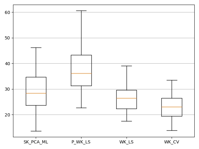
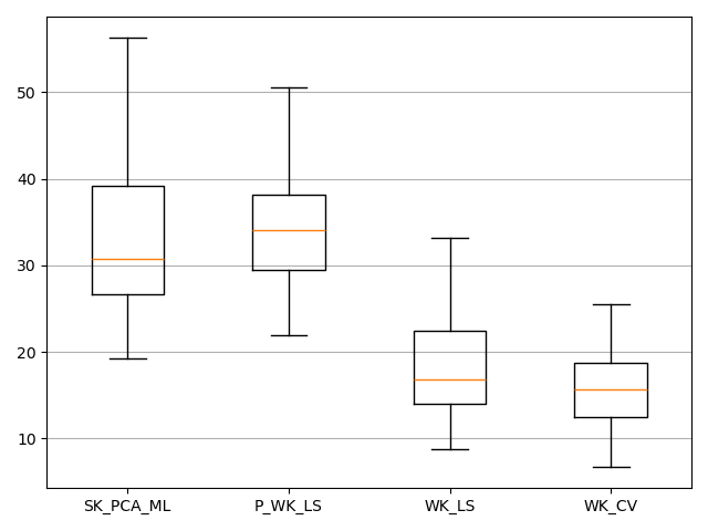
We observe on these figures that the errors produced by the second method (PKW_LS) are significantly larger than those of the other approaches. These results suggest that, for this dataset, the positivity constraint imposed on the weights is too restrictive, especially given that the same model, when applied without this constraint, yields substantially better performances.

Regarding the remaining models, we observe that the two methods based on probability Kriging (KW_LS and KW_CV) outperform the classical Kriging approach in $\mathbb{R}$ especially on the prediction of the 95% quantile. Furthermore, the final and most notable observation is that the probability-measure Kriging model with parameter estimation via cross-validation (KW_CV) consistently achieves the best performances across all quantities of interest.

References

- [1] Luigi Ambrosio, Nicola Gigli, and Giuseppe Savaré. Gradient flows: in metric spaces and in the space of probability measures. Birkhauser, 2008.
- [2] François Bachoc. Cross validation and maximum likelihood estimations of hyper-parameters of Gaussian processes with model misspecification. Computational Statistics & Data Analysis, 66:55–69, 2013.
- [3] Antonio Balzanella and Antonio Irpino. Spatial prediction and spatial dependence monitoring on georeferenced data streams. Statistical Methods and Applications, 29:101–128, 3 2020.
- [4] Randal J. Barnes and Thys B. Johnson. Positive Kriging. Springer Netherlands, Dordrecht, 1984.
- [5] S. Bascou, O. De Luze, S. Ederli, and G. Guillard. Development and validation of the multi-physics draccar code. Annals of Nuclear Energy, 84:1–18, 10 2015.
- [6] Nicolas Bonneel, Gabriel Peyré, and Marco Cuturi. Wasserstein barycentric coordinates: histogram regression using optimal transport. ACM Trans. Graph., 35(4):71–1, 2016.
- [7] William Caballero, Ramón Giraldo, and Jorge Mateu. A universal kriging approach for spatial functional data. Stochastic environmental research and risk assessment, 27(7):1553–1563, 2013.
- [8] Sinho Chewi, Julien Clancy, Thibaut Le Gouic, Philippe Rigollet, George Stepaniants, and Austin Stromme. Fast and smooth interpolation on Wasserstein space. In Proceedings of The 24th International Conference on Artificial Intelligence and Statistics, pages 3061–3069, 2021.
- [9] Noel A.C. Cressie. Statistics for spatial data revised edition. wiley, 4 2015.
- [10] Pedro Delicado, Ramón Giraldo, Carlos Comas, and Jorge Mateu. Statistics for spatial functional data: Some recent contributions. Environmetrics: The official journal of the International Environmetrics Society, 21(3-4):224–239, 2010.
- [11] Olivier Dubrule. Cross validation of Kriging in a unique neighborhood. Journal of the International Association for Mathematical Geology, 15:687–699, 12 1983.
- [12] David Ginsbourger and Cédric Schärer. Fast calculation of Gaussian process multiple-fold cross-validation residuals and their covariances. Journal of Computational and Graphical Statistics, 34:1–14, 1 2021.
- [13] Pierre Goovaerts. Geostatistics for Natural Resources Evaluation. Oxford University Press , 1997.
- [14] R. Gouet, A. López, and J. M. Ortiz. Geodesic Kriging in the Wasserstein space. In Proceedings of the 17th Annual Conference of the International Association for Mathematical Geosciences IAMG, 2015.
- [15] Romain Hug, Emmanuel Maitre, and Nicolas Papadakis. Multi-physics optimal transportation and image interpolation. ESAIM: Mathematical Modelling and Numerical Analysis, 49(6):1671–1692, 2015.
- [16] Sébastien Marmin, David Ginsbourger, Jean Baccou, and Jacques Liandrat. Warped Gaussian processes and derivative-based sequential designs for functions with heterogeneous variations. SIAM/ASA Journal on Uncertainty Quantification, 6(3):991–1018, 2018.
- [17] Amandine Marrel, Bertrand Iooss, Michel Jullien, Béatrice Laurent, and Elena Volkova. Global sensitivity analysis for models with spatially dependent outputs. Environmetrics, 22(3):383–397, 2011.
- [18] Amandine Marrel, Bertrand Iooss, Béatrice Laurent, and Olivier Roustant. Calculations of Sobol indices for the Gaussian process metamodel. Reliability Engineering and System Safety, 94:742–751, 2 2008.
- [19] Alessandra Menafoglio and Piercesare Secchi. Statistical analysis of complex and spatially dependent data: A review of object oriented spatial statistics. European Journal of Operational Research, 258:401–410, 4 2017.
- [20] Alessandra Menafoglio, Piercesare Secchi, and Matilde Dalla Rosa. A Universal Kriging predictor for spatially dependent functional data of a Hilbert Space. Electronic Journal of Statistics, 7:2209–2240, 2013.
- [21] Carl Edward Rasmussen and Christopher K. I. Williams. Gaussian Processes for Machine Learning. The MIT Press, 2006.
- [22] Filippo Santambrogio. Optimal transport for applied mathematicians. Springer International Publishing, 87, 2015.
- [23] Michael L. Stein. Interpolation of spatial data : some theory for Kriging. Springer, 1999.
- [24] Fuzhen Zhang. The Schur Complement and Its Applications. Springer-Verlag, 2005.