跳到论文正文
W Papers独立论文阅读器 arXiv:2510.20246 论文正文 计算阅读时间 · 0%
引用这篇论文根据当前论文元数据生成,正式投稿前建议核对。


License: arXiv.org perpetual non-exclusive license
arXiv:2510.20246v2 [math.OC] 26 May 2026

Convergence Analysis of Noisy Distributed Gradient Descent for Non-convex Optimization — Saddle Point Escape

Lei Qin    Michael Cantoni    Member    IEEE    and Ye Pu    Member    IEEE This work was supported by a Melbourne Research Scholarship and the Australian Research Council (DE220101527 and DP210103272).L. Qin, M. Cantoni, and Y. Pu are with the Department of Electrical and Electronic Engineering, University of Melbourne, Parkville VIC 3010, Australia leqin@student.unimelb.edu.au, {cantoni, ye.pu}@unimelb.edu.au.
Abstract

This paper studies a noisy variant of consensus-based distributed gradient descent (DGD) for minimizing finite sums of smooth but possibly non-convex functions over a network. By introducing stochastic perturbations into the local gradient updates, the proposed noisy distributed gradient descent (NDGD) algorithm enables escape from saddle points while preserving distributed implementation and consensus structure. Under mild regularity conditions and sufficiently small step-size and noise variance, it is shown that the iterates of all agents converge with high probability to a neighborhood of a common local minimizer. In addition, the proposed method achieves convergence complexity comparable to centralized first-order saddle-point escape methods, reducing exponential dependence on problem dimension to polynomial dependence, which is particularly important in distributed optimization where the overall problem dimension scales with both the local dimension and the number of agents. Numerical experiments demonstrate that NDGD outperforms standard DGD in escaping saddle points and achieving improved solution quality in non-convex settings.

{IEEEkeywords}

Non-convex optimization; consensus-based distributed optimization; first-order methods; random perturbations; escaping saddle points

1 Introduction

Collaborative distributed optimization across networks has attracted significant attention due to its applications in large-scale engineered systems, including multi-agent control [16, 15, 3], sensor networks [23, 12], and machine learning [2, 13, 14]. In particular, such frameworks provide guidance for practical applications such as distributed model predictive control (MPC), multi-agent reinforcement learning (RL), and large-scale resource allocation in networked systems, where coordinated decision-making is required.

We consider objective functions of the form

f​(𝐱)=∑i=1mfi​(𝐱),\displaystyle f(\mathbf{x})=\sum\nolimits_{i=1}^{m}f_{i}(\mathbf{x}), (1)

where each fi:ℝn→ℝf_{i}\mathrel{\mathop{\ordinarycolon}}\mathbb{R}^{n}\rightarrow\mathbb{R} is smooth but potentially non-convex. The goal is to design a distributed algorithm that enables mm agents to collaboratively compute a second-order stationary point of (1). Agents communicate over an undirected graph 𝒢​(𝒱,ℰ)\mathcal{G}(\mathcal{V},\mathcal{E}), where each agent ii has access only to fif_{i} and exchanges information with its neighbors.

We study a perturbed variant of consensus-based distributed gradient descent (DGD) [19]. To overcome saddle-point stagnation in non-convex settings, random perturbations are injected into the iterates. Our preliminary work [20] considered this idea under more restrictive assumptions. The update for agent ii at iteration kk is

𝐱^ik+1=∑j=1mwi​j​𝐱^jk−α​(∇fi​(𝐱^ik)+𝐧ik),\displaystyle\hat{\mathbf{x}}^{k+1}_{i}=\sum\nolimits_{j=1}^{m}w_{ij}\hat{\mathbf{x}}^{k}_{j}-\alpha(\nabla f_{i}(\hat{\mathbf{x}}^{k}_{i})+\mathbf{n}_{i}^{k}), (2)

where α>0\alpha>0 is a fixed step-size, 𝐖\mathbf{W} is the mixing matrix, and 𝐧ik\mathbf{n}_{i}^{k} is a stochastic perturbation. We refer to this algorithm as NDGD. A constant step-size is adopted to simplify analysis and enable explicit characterization of the trade-off between convergence accuracy and robustness to noise, which is essential for establishing second-order guarantees. The key challenge lies in characterizing saddle point escape in the presence of consensus dynamics and network-induced coupling, where local perturbations interact with global agreement constraints.

1.1 Main contributions

  • •

    Under suitable first- and second-order regularity conditions, we show that, with sufficiently small step-size and noise variance, the iterates converge with high probability to a neighborhood of a local minimizer of (1) (Theorem 3.2), jointly capturing optimality gap and consensus error.

  • •

    We establish finite-time convergence rates comparable to centralized smooth non-convex optimization, highlighting the roles of step-size, noise, and network structure.

  • •

    Numerical experiments demonstrate improved saddle-point escape over standard DGD, while maintaining stable convergence and consensus (Section 4).

Our analysis reformulates NDGD in a lifted centralized form, enabling the use of classical gradient dynamics. By combining this with concentration inequalities for stochastic increments, we establish convergence to approximate second-order stationary points with probabilistic guarantees.

1.2 Related work

DGD, introduced in [19], is a fundamental consensus-based method where agents combine local gradient steps with neighbor averaging. Dual-decomposition methods [28] offer an alternative but typically incur higher communication costs.

Variants of DGD have been extensively studied [18, 9]. While diminishing step-sizes are commonly used, gradient tracking enables exact convergence with constant step-size [24, 17, 5, 6]. Convergence guarantees for convex settings are well established [34, 29, 22], and have been extended to relaxed assumptions [33]. For non-convex problems, DGD converges to first-order stationary points [35], but these may include saddle points.

Although saddle points are almost surely avoided under certain conditions [4, 26, 27, 21], escaping them can require exponential time in worst-case scenarios [7]. While second-order methods can address this issue, they are typically impractical in distributed settings due to their computational cost.

Recent work introduces perturbations to enable efficient saddle-point escape. Building on centralized results [8, 10, 11], distributed variants inject noise into gradient updates. Prior work [30, 31] shows that average iterates may approach second-order stationary points, but does not guarantee convergence of individual agents. More recent approaches [32, 1] improve performance but rely on diminishing step-sizes. Our prior work [20] combines lifting techniques [34, 35, 4] with stochastic analysis to establish convergence guarantees. The present paper further strengthens these results by refining rate bounds and explicitly characterizing local regularity conditions.

1.3 Notation

Let 𝐈n\mathbf{I}_{n} denote the n×nn\times n identity matrix, 𝟏n\bm{1}_{n} denote the nn-vector with all entries equal to 11, and both 𝐀i​j\mathbf{A}_{ij} and ai​ja_{ij} denote the entry in row ii and column jj of the matrix 𝐀\mathbf{A}. For a square symmetric matrix 𝐁\mathbf{B}, the eigenvalues are real valued, and we use λmin​(𝐁)\lambda_{\mathrm{min}}(\mathbf{B}), λmax​(𝐁)\lambda_{\mathrm{max}}(\mathbf{B}), and ‖𝐁‖\|\mathbf{B}\| to denote the minimum eigenvalue, maximum eigenvalue, and spectral norm, respectively. Further, 𝐁1≺(resp.⪯)𝐁2\mathbf{B}_{1}\prec(\mathrm{resp.}\preceq)\,\mathbf{B}_{2} is equivalent to λmin(𝐁2−𝐁1)>(resp.≥) 0\lambda_{\mathrm{min}}(\mathbf{B}_{2}-\mathbf{B}_{1})>(\mathrm{resp.}\geq)\,0. The Kronecker product is denoted by ⊗\otimes. The distance from the point 𝐱∈ℝn\mathbf{x}\in\mathbb{R}^{n} to a given set 𝒴⊆ℝn\mathcal{Y}\subseteq\mathbb{R}^{n} is denoted by dist​(𝐱,𝒴)≔inf𝐲∈𝒴‖𝐱−𝐲‖\textup{dist}(\mathbf{x},\mathcal{Y})\coloneqq\inf_{\mathbf{y}\in\mathcal{Y}}\|\mathbf{x}-\mathbf{y}\|. We say that a point 𝐱\mathbf{x} is δ\delta-close to a point 𝐲\mathbf{y} (resp., a set 𝒴\mathcal{Y}) if ‖𝐱−𝐲‖≤δ\|\mathbf{x}-\mathbf{y}\|\leq\delta (resp., dist​(𝐱,𝒴)≤δ\textup{dist}(\mathbf{x},\mathcal{Y})\leq\delta). Let 𝐱∼𝒩​(𝝁,𝚺)\mathbf{x}\sim\mathcal{N}(\bm{\mu},\bm{\Sigma}) denote the multivariate normal distribution of a nn-dimensional random vector 𝐱∈ℝn\mathbf{x}\in\mathbb{R}^{n} with mean 𝝁∈ℝn\bm{\mu}\in\mathbb{R}^{n} and variance 𝚺∈ℝn×n\bm{\Sigma}\in\mathbb{R}^{n\times n}. Let 𝔼\mathbb{E} and ℙ\mathbb{P} denote the expectation and probability operators, respectively. Let ⌈⋅⌉\lceil\cdot\rceil denote the ceiling function. Unless stated otherwise, all iteration indices are positive integers, and superscript indexing is used to denote iterates.

2 Assumptions and Preliminary Results

This section contains a summary of basic definitions, assumptions, and two preliminary results pertaining to the aforementioned lifting approach within the context of standard (noise free) fixed step-size DGD. The second result relates the local minimizers of (1) to those of a lifted representation of this objective function, under local regularity conditions that are directly formulated in terms of the component functions fif_{i}. The relationships underpin the subsequent development of the main results on NDGD, in which the gradient is randomly perturbed at each iteration as per (2). The complete proof is provided in [21, Section IV-A].

2.1 Definitions and Assumptions

Definition 2.1 (First order stationarity).

For differentiable function h:ℝn→ℝh\mathrel{\mathop{\ordinarycolon}}\mathbb{R}^{n}\rightarrow\mathbb{R}, the point 𝐱\mathbf{x} is said to be first-order stationary if ‖∇h​(𝐱)‖=0\|\nabla h(\mathbf{x})\|=0, where ∇h:ℝn→ℝn\nabla h\mathrel{\mathop{\ordinarycolon}}\mathbb{R}^{n}\rightarrow\mathbb{R}^{n} denotes the gradient of hh.

Definition 2.2 (Second order stationarity).

For twice differentiable function h:ℝn→ℝh\mathrel{\mathop{\ordinarycolon}}\mathbb{R}^{n}\rightarrow\mathbb{R}, a first-order stationary point 𝐱\mathbf{x} is: (i) a local minimizer, if ∇2h​(𝐱)≻𝟎\nabla^{2}h(\mathbf{x})\succ\bm{0}; (ii) a local maximizer, if ∇2h​(𝐱)≺𝟎\nabla^{2}h(\mathbf{x})\prec\bm{0}; and (iii) a strict saddle point if λmin​(∇2h​(𝐱))<0\lambda_{\min}(\nabla^{2}h(\mathbf{x}))<0 and λmax​(∇2h​(𝐱))>0\lambda_{\max}(\nabla^{2}h(\mathbf{x}))>0, where ∇2h:ℝn→ℝn×n\nabla^{2}h\mathrel{\mathop{\ordinarycolon}}\mathbb{R}^{n}\rightarrow\mathbb{R}^{n\times n} denotes the Hessian of hh.

Assumption 2.1 (Strict saddle).

The function f:ℝn→ℝf\mathrel{\mathop{\ordinarycolon}}\mathbb{R}^{n}\rightarrow\mathbb{R} in (1) is such that for all first-order stationary points 𝐱\mathbf{x}, either λmin​(∇2f​(𝐱))>0\lambda_{\min}(\nabla^{2}f(\mathbf{x}))>0 (i.e., 𝐱\mathbf{x} is a local minimizer), or λmin​(∇2f​(𝐱))<0\lambda_{\min}(\nabla^{2}f(\mathbf{x}))<0 (i.e., 𝐱\mathbf{x} is a saddle point or a maximizer).

Assumption 2.2 (Lipschitz continuity).

Each fif_{i} in (1) is both LfigL_{f_{i}}^{g}-gradient Lipschitz and LfiHL_{f_{i}}^{H}-Hessian Lipschitz, i.e., for all 𝐱,𝐲∈ℝn\mathbf{x},\mathbf{y}\in\mathbb{R}^{n}, and each i∈𝒱i\in\mathcal{V}, ‖∇fi​(𝐱)−∇fi​(𝐲)‖≤Lfig​‖𝐱−𝐲‖\|\nabla f_{i}(\mathbf{x})-\nabla f_{i}(\mathbf{y})\|\leq L_{f_{i}}^{g}\|\mathbf{x}-\mathbf{y}\| and ‖∇2fi​(𝐱)−∇2fi​(𝐲)‖≤LfiH​‖𝐱−𝐲‖\|\nabla^{2}f_{i}(\mathbf{x})-\nabla^{2}f_{i}(\mathbf{y})\|\leq L_{f_{i}}^{H}\|\mathbf{x}-\mathbf{y}\|.

Assumption 2.3 (Coercivity).

Each fif_{i} in (1) is coercive (i.e., fi​(𝐱)→∞f_{i}(\mathbf{x})\rightarrow\infty as ‖𝐱‖→∞\|\mathbf{x}\|\rightarrow\infty, which is equivalent to compactness of all sublevel sets by continuity), and ‖∇f‖\|\nabla f\| is also coercive.

Remark 1.

Coercivity of ‖∇f‖\|\nabla f\| is commonly satisfied in optimization. In particular, adding a regularization term of the form λ2​‖𝐱‖2\frac{\lambda}{2}\|\mathbf{x}\|^{2} to the objective function ensures this condition.

Assumption 2.4 (Bounded gradient disagreement).

There exists constant D>0D>0 such that for and two agents i,j∈𝒱i,j\in\mathcal{V}, and every 𝐱∈ℝn\mathbf{x}\in\mathbb{R}^{n}, fif_{i} and fjf_{j} in (1) satisfy ‖∇fi​(𝐱)−∇fj​(𝐱)‖≤D\|\nabla f_{i}(\mathbf{x})-\nabla f_{j}(\mathbf{x})\|\leq D.

Remark 2.

Assumption 2.4 is weaker than the more common assumption of uniformly bounded gradients. It can be satisfied when all agents are minimizing the same cost function with the same regularizers, with different parameters. For further discussions, see [30] and [25].

Assumption 2.5 (Connected network).

The undirected graph 𝒢​(𝒱,ℰ)\mathcal{G}(\mathcal{V},\mathcal{E}) is connected.

Assumption 2.6 (Mixing matrix).

The mixing matrix 𝐖∈ℝm×m\mathbf{W}\in\mathbb{R}^{m\times m} relating to the agent iteration (2), satisfies the following conditions:

  1. i)

    𝐖\mathbf{W} is consistent with the graph 𝒢​(𝒱,ℰ)\mathcal{G}(\mathcal{V},\mathcal{E}) in the sense that wi​i>0w_{ii}>0 for all i∈𝒱i\in\mathcal{V}, wi​j>0w_{ij}>0 if (i,j)∈ℰ(i,j)\in\mathcal{E}, and wi​j=0w_{ij}=0 otherwise.

  2. ii)

    𝐖=𝐖⊤\mathbf{W}=\mathbf{W}^{\top};

  3. iii)

    null​{𝐈m−𝐖}=span​{𝟏m}\textup{null}\{\mathbf{I}_{m}-\mathbf{W}\}=\textup{span}\{\bm{1}_{m}\};

  4. iv)

    𝟎≺𝐖⪯𝐈m\bm{0}\prec\mathbf{W}\preceq\mathbf{I}_{m}.

Remark 3.

Conditions ii), iii), and iv) in Assumption 2.6 are satisfied if 𝐖\mathbf{W} is a symmetric doubly stochastic matrix. In particular, this implies that 𝐖​𝟏m=𝟏m\mathbf{W}\bm{1}_{m}=\bm{1}_{m} and 𝟏m⊤​𝐖=𝟏m⊤\bm{1}_{m}^{\top}\mathbf{W}=\bm{1}_{m}^{\top}.

Assumption 2.7 (Random perturbation).

Given σ>0\sigma>0, for each k>0k>0, and i∈𝒱i\in\mathcal{V}, the random perturbation 𝐧ik\mathbf{n}_{i}^{k} in (2) satisfies that 𝐧ik∼𝒩​(𝟎,σ2​𝐈n)\mathbf{n}_{i}^{k}\sim\mathcal{N}(\bm{0},\sigma^{2}\mathbf{I}_{n}).

Remark 4.

If Assumption 2.7 holds, then for each k>0k>0, the random perturbation

𝐧k=[(𝐧1k)⊤,⋯,(𝐧mk)⊤]⊤∈(ℝn)m\displaystyle\mathbf{n}^{k}=[(\mathbf{n}_{1}^{k})^{\top},\cdots,(\mathbf{n}_{m}^{k})^{\top}]^{\top}\in(\mathbb{R}^{n})^{m}

is i.i.d satisfying 𝐧k∼𝒩​(𝟎,σ2​𝐈m​n)\mathbf{n}^{k}\sim\mathcal{N}(\bm{0},\sigma^{2}\mathbf{I}_{mn}) and the expected value 𝔼​[‖𝐧k‖2]=m​n​σ2\mathbb{E}[\|\mathbf{n}^{k}\|^{2}]=mn\sigma^{2}.

2.2 Distributed Gradient Descent

In this section, we examine the standard DGD algorithm through the lens of an auxiliary function in a lifted setting. This methodology is subsequently applied to NDGD with random perturbations as per (2). We first introduce the lifted objective function

F​(𝐱^)=∑i=1mfi​(𝐱^i),\displaystyle\begin{gathered}F(\hat{\mathbf{x}})=\sum_{i=1}^{m}f_{i}(\hat{\mathbf{x}}_{i}),\end{gathered} (4)

where 𝐱^=[𝐱^1⊤,⋯,𝐱^m⊤]⊤∈(ℝn)m\hat{\mathbf{x}}=[\hat{\mathbf{x}}_{1}^{\top},\cdots,\hat{\mathbf{x}}_{m}^{\top}]^{\top}\in(\mathbb{R}^{n})^{m} is the stacked vector collecting the local copies 𝐱^i∈ℝn\hat{\mathbf{x}}_{i}\in\mathbb{R}^{n} maintained by the mm agents. Note that, ∇F​(𝐱^)=[∇f1​(𝐱^1)⊤,⋯,∇fm​(𝐱^m)⊤]⊤\nabla F(\hat{\mathbf{x}})=[\nabla f_{1}(\hat{\mathbf{x}}_{1})^{\top},\cdots,\nabla f_{m}(\hat{\mathbf{x}}_{m})^{\top}]^{\top} and ∇2F​(𝐱^)=⨁i=1m∇2fi​(𝐱^i)\nabla^{2}F(\hat{\mathbf{x}})=\bigoplus_{i=1}^{m}\nabla^{2}f_{i}(\hat{\mathbf{x}}_{i}). In particular, ∇2F\nabla^{2}F is block diagonal.

Remark 5.

The following constants are introduced for later use for the convergence analysis in Section 3. If Assumption 2.2 holds, then FF defined in (4) has LFgL_{F}^{g}-Lipschitz continuous gradient and LFHL_{F}^{H}-Lipschitz continuous Hessian with

LFg=maxi⁡{Lfig},LFH=maxi⁡{LfiH}.\displaystyle L_{F}^{g}=\max_{i}\{L_{f_{i}}^{g}\},\qquad L_{F}^{H}=\max_{i}\{L_{f_{i}}^{H}\}.
Definition 2.3 (Consensual first order stationarity).

For F:(ℝn)m→ℝF\mathrel{\mathop{\ordinarycolon}}(\mathbb{R}^{n})^{m}\rightarrow\mathbb{R} in (4), the point 𝐱^∈(ℝn)m\hat{\mathbf{x}}\in(\mathbb{R}^{n})^{m} is said to be a consensual first order stationary point if it satisfies following conditions:

  1. i)

    𝐱^=𝟏m⊗av⁡(𝐱^)\hat{\mathbf{x}}=\bm{1}_{m}\otimes\operatorname{av}(\hat{\mathbf{x}}) where

    av⁡(𝐱^)=1m​(𝟏m⊗𝐈n)⊤​𝐱^∈ℝn;\displaystyle\operatorname{av}(\hat{\mathbf{x}})=\frac{1}{m}(\bm{1}_{m}\otimes\mathbf{I}_{n})^{\top}\hat{\mathbf{x}}\in\mathbb{R}^{n}; (5)
  2. ii)

    (𝟏m⊗𝐈n)⊤​∇F​(𝐱^)=∑i=1m∇fi​(𝐱^i)=𝟎(\bm{1}_{m}\otimes\mathbf{I}_{n})^{\top}\nabla F(\hat{\mathbf{x}})=\sum_{i=1}^{m}\nabla f_{i}(\hat{\mathbf{x}}_{i})=\bm{0}.

If condition i) holds, then 𝐱^\hat{\mathbf{x}} is in consensus, in the following sense: 𝐱^i=𝐱^j\hat{\mathbf{x}}_{i}=\hat{\mathbf{x}}_{j} for all ii, j∈𝒱j\in\mathcal{V}. Further, if condition ii) also holds, then for every i∈𝒱i\in\mathcal{V}, the point 𝐱^i\hat{\mathbf{x}}_{i} is first-order stationary for ff.

Definition 2.4 (Consensual second-order stationarity).

For F:(ℝn)m→ℝF\mathrel{\mathop{\ordinarycolon}}(\mathbb{R}^{n})^{m}\rightarrow\mathbb{R} in (4), the point 𝐱^∈(ℝn)m\hat{\mathbf{x}}\in(\mathbb{R}^{n})^{m} is said to be a (η,ϵ,γ)(\eta,\epsilon,\gamma)-consensual second-order stationary point if it satisfies the following:

  1. i)

    ‖𝐱^−𝟏m⊗av⁡(𝐱^)‖≤η\|\hat{\mathbf{x}}-\bm{1}_{m}\otimes\operatorname{av}(\hat{\mathbf{x}})\|\leq\eta with av⁡(⋅)\operatorname{av}(\cdot) as per (5);

  2. ii)

    ‖(𝟏m⊗𝐈n)⊤​∇F​(𝐱^)‖=‖∑i=1m∇fi​(𝐱^i)‖≤ϵ\|(\bm{1}_{m}\otimes\mathbf{I}_{n})^{\top}\nabla F(\hat{\mathbf{x}})\|=\|\sum_{i=1}^{m}\nabla f_{i}(\hat{\mathbf{x}}_{i})\|\leq\epsilon;

  3. iii)

    λmin​(H​(𝐱^))=λmin​(∑i=1m∇2fi​(𝐱^i))≥−γ\lambda_{\min}(H(\hat{\mathbf{x}}))=\lambda_{\min}(\sum_{i=1}^{m}\nabla^{2}f_{i}(\hat{\mathbf{x}}_{i}))\geq-\gamma, where H​(𝐱^)=(𝟏m⊗𝐈n)⊤​∇2F​(𝐱^)​(𝟏m⊗𝐈n)H(\hat{\mathbf{x}})=(\bm{1}_{m}\otimes\mathbf{I}_{n})^{\top}\nabla^{2}F(\hat{\mathbf{x}})(\bm{1}_{m}\otimes\mathbf{I}_{n}).

Recall the standard fixed step-size DGD algorithm [19]:

𝐱^ik+1=∑j=1mwi​j​𝐱^jk−α​∇fi​(𝐱^ik),\displaystyle\hat{\mathbf{x}}^{k+1}_{i}=\sum_{j=1}^{m}w_{ij}\hat{\mathbf{x}}^{k}_{j}-\alpha\nabla f_{i}(\hat{\mathbf{x}}^{k}_{i}),

for i∈𝒱i\in\mathcal{V}, with α>0\alpha>0. In aggregate, this can be re-written as

𝐱^k+1=𝐖^​𝐱^k−α​∇F​(𝐱^k),\displaystyle\hat{\mathbf{x}}^{k+1}=\hat{\mathbf{W}}\hat{\mathbf{x}}^{k}-\alpha\nabla F(\hat{\mathbf{x}}^{k}), (6)

where 𝐖^:=𝐖⊗𝐈n\hat{\mathbf{W}}\mathrel{\mathop{\ordinarycolon}}=\mathbf{W}\otimes\mathbf{I}_{n}. As proposed in some earlier works, including [34, 35, 4], the convergence properties can be studied via an auxiliary function

Qα​(𝐱^)=∑i=1mfi​(𝐱^i)+12​α​∑i=1m∑j=1m(𝐈m−𝐖)i​j​(𝐱^i)⊤​(𝐱^j)=F​(𝐱^)+12​α​‖𝐱^‖𝐈m​n−𝐖^2,\displaystyle\begin{aligned} Q_{\alpha}(\hat{\mathbf{x}})&=\sum_{i=1}^{m}f_{i}(\hat{\mathbf{x}}_{i})+\frac{1}{2\alpha}\sum_{i=1}^{m}\sum_{j=1}^{m}(\mathbf{I}_{m}-\mathbf{W})_{ij}(\hat{\mathbf{x}}_{i})^{\top}(\hat{\mathbf{x}}_{j})\\ &=F(\hat{\mathbf{x}})+\frac{1}{2\alpha}\|\hat{\mathbf{x}}\|^{2}_{\mathbf{I}_{mn}-\hat{\mathbf{W}}},\end{aligned} (7)

which consists of the objective function in (4) and a quadratic penalty, which depends on the step-size and the mixing matrix. The DGD update (6) for (4) can be interpreted as an instance of the standard gradient descent algorithm applied to (7), i.e.,

𝐱^k+1=𝐱^k−α​∇Qα​(𝐱^k).\displaystyle\hat{\mathbf{x}}^{k+1}=\hat{\mathbf{x}}^{k}-\alpha\nabla Q_{\alpha}(\hat{\mathbf{x}}^{k}). (8)

Iterating (6) and (8) from the same initialization yields the same sequence of iterates; see [35, Lemma 1]. Similarly, the NDGD update (2) for (4) can be interpreted as an instance of the noisy gradient descent algorithm applied to (7), i.e.,

𝐱^k+1=𝐱^k−α​(∇Qα​(𝐱^k)+𝐧k).\displaystyle\hat{\mathbf{x}}^{k+1}=\hat{\mathbf{x}}^{k}-\alpha(\nabla Q_{\alpha}(\hat{\mathbf{x}}^{k})+\mathbf{n}^{k}). (9)
Remark 6.

If Assumption 2.2 holds, with LFgL_{F}^{g} and LFHL_{F}^{H} defined in Remark 5, then QαQ_{\alpha} in (7) has LQαgL_{Q_{\alpha}}^{g}-Lipschitz continuous gradient and LQαHL_{Q_{\alpha}}^{H}-Lipschitz continuous Hessian, where

LQαg=LFg+α−1​(1−λmin​(𝐖)),andLQαH=LFH.\displaystyle L_{Q_{\alpha}}^{g}=L_{F}^{g}+\alpha^{-1}(1-\lambda_{\min}(\mathbf{W})),\quad\text{and}\quad L_{Q_{\alpha}}^{H}=L_{F}^{H}.
Remark 7.

If Assumption 2.3 holds, then for any fixed α>0\alpha>0, QαQ_{\alpha} is coercive. In particular, for all c>0c>0, the sublevel set 𝒮c={𝐱^∈(ℝn)m:Qα​(𝐱^)≤c}\mathcal{S}_{c}=\{\hat{\mathbf{x}}\in(\mathbb{R}^{n})^{m}\mathrel{\mathop{\ordinarycolon}}Q_{\alpha}(\hat{\mathbf{x}})\leq c\} is contained inside the set 𝒮c′={𝐱^∈(ℝn)m:F​(𝐱^)≤c}\mathcal{S}_{c}^{\prime}=\{\hat{\mathbf{x}}\in(\mathbb{R}^{n})^{m}\mathrel{\mathop{\ordinarycolon}}F(\hat{\mathbf{x}})\leq c\}, since 12​α​‖𝐱^‖𝐈m​n−𝐖^2≥0\frac{1}{2\alpha}\|\hat{\mathbf{x}}\|^{2}_{\mathbf{I}_{mn}-\hat{\mathbf{W}}}\geq 0, i.e., 𝒮c⊆𝒮c′\mathcal{S}_{c}\subseteq\mathcal{S}_{c}^{\prime}. By Assumption 2.3, FF is coercive, whereby every 𝒮c′\mathcal{S}_{c}^{\prime} is compact by continuity, and therefore, each closed subset 𝒮c\mathcal{S}_{c} is bounded. Thus, QαQ_{\alpha} is coercive.

Definition 2.5 (Local minimizers).

Let 𝒳f⋆\mathcal{X}_{f}^{\star} and 𝒳Qα⋆\mathcal{X}_{Q_{\alpha}}^{\star} denote the sets of local minimizers of ff and QαQ_{\alpha}, respectively:

𝒳f⋆={𝐱∈ℝn:∇f(𝐱)=𝟎,∇2f(𝐱)≻𝟎},𝒳Qα⋆={𝐱^∈(ℝn)m:∇Qα(𝐱^)=𝟎,∇2Qα(𝐱^)≻𝟎}.\displaystyle\begin{aligned} \mathcal{X}_{f}^{\star}=\{\mathbf{x}\in\mathbb{R}^{n}\mathrel{\mathop{\ordinarycolon}}&~\nabla f(\mathbf{x})=\bm{0},~\nabla^{2}f(\mathbf{x})\succ\bm{0}\},\\ \mathcal{X}_{Q_{\alpha}}^{\star}=\{\hat{\mathbf{x}}\in(\mathbb{R}^{n})^{m}\mathrel{\mathop{\ordinarycolon}}&~\nabla Q_{\alpha}(\hat{\mathbf{x}})=\bm{0},~\nabla^{2}Q_{\alpha}(\hat{\mathbf{x}})\succ\bm{0}\}.\end{aligned} (10)

Next, we establish a second-order relationship between FF and QαQ_{\alpha}. The complete proof is provided in [21, Section II-B].

Lemma 2.1.

Given any α>0\alpha>0, for all 𝐱^∈(ℝn)m\hat{\mathbf{x}}\in(\mathbb{R}^{n})^{m},

λmin​(∇2F​(𝐱^))≤λmin​(∇2Qα​(𝐱^))≤1m​λmin​(∑i=1m∇2fi​(𝐱^i)).\displaystyle\lambda_{\min}(\nabla^{2}F(\hat{\mathbf{x}}))\leq\lambda_{\min}(\nabla^{2}Q_{\alpha}(\hat{\mathbf{x}}))\leq\frac{1}{m}\lambda_{\min}(\sum_{i=1}^{m}\nabla^{2}f_{i}(\hat{\mathbf{x}}_{i})).

2.3 Relationships Between Local Minimizers of f and Qα

In this section, additional regularity conditions on ff are introduced. These local conditions are formulated from the perspective of ensuring the ii-th component 𝐱^i⋆\hat{\mathbf{x}}_{i}^{\star} of a local minimizer 𝐱^⋆∈𝒳Qα⋆\hat{\mathbf{x}}^{\star}\in\mathcal{X}_{Q_{\alpha}}^{\star}, can be made arbitrarily close to the set 𝒳f⋆\mathcal{X}_{f}^{\star} by the selection of a sufficiently small step-size α>0\alpha>0. This expands upon the results in [4] regarding the relationship between first order stationary points of ff and QαQ_{\alpha}.

Assumption 2.8 (Local regularity).

There exist positive constants α′,γ,δ,ϵ,η,μ>0\alpha^{\prime},~\gamma,~\delta,~\epsilon,~\eta,~\mu>0 such that for any point 𝐱^=[𝐱^1⊤,⋯,𝐱^m⊤]⊤∈(ℝn)m\hat{\mathbf{x}}=[\hat{\mathbf{x}}_{1}^{\top},\cdots,\hat{\mathbf{x}}_{m}^{\top}]^{\top}\in(\mathbb{R}^{n})^{m} satisfying ‖𝐱^−𝟏m⊗av⁡(𝐱^)‖≤η\|\hat{\mathbf{x}}-\bm{1}_{m}\otimes\operatorname{av}(\hat{\mathbf{x}})\|\leq\eta, with av⁡(⋅)\operatorname{av}(\cdot) as per (5), at least one of the following is true:

  1. i)

    ‖∑i=1m∇fi​(𝐱^i)‖>ϵ\|\sum_{i=1}^{m}\nabla f_{i}(\hat{\mathbf{x}}_{i})\|>\epsilon;

  2. ii)

    λmin​(∑i=1m∇2fi​(𝐱^i))<−γ\lambda_{\min}(\sum_{i=1}^{m}\nabla^{2}f_{i}(\hat{\mathbf{x}}_{i}))<-\gamma;

  3. iii)

    for all 0<α≤α′0<\alpha\leq\alpha^{\prime}, there exists 𝐱^′∈(ℝn)m\hat{\mathbf{x}}^{\prime}\in(\mathbb{R}^{n})^{m} such that ‖𝐱^′−𝐱^‖≤δ\|\hat{\mathbf{x}}^{\prime}-\hat{\mathbf{x}}\|\leq\delta, ∑j=1mwi​j​(𝐱^j′−𝐱^i′)=α​∇fi​(𝐱^i′)​ for all ​i∈𝒱\sum_{j=1}^{m}w_{ij}(\hat{\mathbf{x}}_{j}^{\prime}-\hat{\mathbf{x}}_{i}^{\prime})=\alpha\nabla f_{i}(\hat{\mathbf{x}}_{i}^{\prime})\text{ for all }i\in\mathcal{V}, and λmin​(∇2F​(𝐲^))≥μ​for all ​𝐲^​ with ​‖𝐲^−𝐱^′‖≤3​δ\lambda_{\min}(\nabla^{2}F(\hat{\mathbf{y}}))\geq\mu~\text{for all }\hat{\mathbf{y}}\text{ with }\|\hat{\mathbf{y}}-\hat{\mathbf{x}}^{\prime}\|\leq 3\delta, i.e., FF is strongly convex in the vicinity of 𝐱^′\hat{\mathbf{x}}^{\prime}.

Intuitively, the first two conditions in Assumption 2.8 relate to points 𝐱^∈(ℝn)m\hat{\mathbf{x}}\in(\mathbb{R}^{n})^{m} with small consensus error, η>0\eta>0, that have significant gradient sum (𝟏m⊗𝐈n)⊤​∇F​(𝐱^)=∑i=1m∇fi​(𝐱^i)(\bm{1}_{m}\otimes\mathbf{I}_{n})^{\top}\nabla F(\hat{\mathbf{x}})=\sum_{i=1}^{m}\nabla f_{i}(\hat{\mathbf{x}}_{i}), exceeding ϵ>0\epsilon>0, or substantially negative Hessian gain in at least one direction, of size exceeding γ>0\gamma>0. If i) fails, it means that in consensus preserving directions, the landscape of FF is flat around 𝐱^\hat{\mathbf{x}}. If ii) fails, it means there is no consensus preserving direction resulting in significant ascent of FF. So if both i) and ii) fail, for all correspondingly consensual second-order stationary points as specified in Definition 2.4, there exists a robust local minimizer of QαQ_{\alpha} in the vicinity of 𝐱^\hat{\mathbf{x}} by condition iii). Assumption 2.8 is only required for the convergence guarantees to a local minimizer in Theorem 3.2, and is not needed for the approximate second-order stationarity result in Theorem 3.1.

Lemma 2.2.

Let Assumptions 2.1, 2.2, 2.3, 2.5, 2.6, 2.8 hold. With α′\alpha^{\prime}, δ\delta, μ>0\mu>0 as per Assumption 2.8, there exists threshold 0<α¯​(δ)≤α′0<\bar{\alpha}(\delta)\leq\alpha^{\prime} such that for every 0<α≤α¯​(δ)0<\alpha\leq\bar{\alpha}(\delta), if

𝐱^⋆∈{𝐱^∈𝒳Qα⋆:‖𝐱^−𝟏m⊗av⁡(𝐱^)‖≤5μ​α},\displaystyle\hat{\mathbf{x}}^{\star}\in\{\hat{\mathbf{x}}\in\mathcal{X}_{Q_{\alpha}}^{\star}\mathrel{\mathop{\ordinarycolon}}~\|\hat{\mathbf{x}}-\bm{1}_{m}\otimes\operatorname{av}(\hat{\mathbf{x}})\|\leq\frac{5}{\mu}\sqrt{\alpha}\}, (11)

with av⁡(⋅)\operatorname{av}(\cdot) as per (5), then for all i∈𝒱i\in\mathcal{V},

dist​(𝐱^i⋆,𝒳f⋆)≤(1+m​LFgμ)​5μ​α.\displaystyle\textup{dist}(\hat{\mathbf{x}}_{i}^{\star},\mathcal{X}_{f}^{\star})\leq(1+\frac{\sqrt{m}L_{F}^{g}}{\mu})\frac{5}{\mu}\sqrt{\alpha}.

The essence of Lemma 2.2 is that under the stated regularity conditions, and with sufficiently small α\alpha, each agent-wise component of a local minimizer of QαQ_{\alpha} that exhibits small consensus error, also lies close to a local minimizer of ff. Later, we will prove the set in (11) is not empty.

3 Main Results

The two main theorems of the paper are presented in this section. Proofs are provided for these via two additional main lemmas. Theorem 3.1 concerns the iterates of (2) and the probability of reaching a neighborhood of a consensual second-order stationary point under correspondingly parametrized step size, noise variance, and consensus error. In Theorem 3.2, probabilistic convergence guarantees are provided for sufficiently small fixed step-size and noise variance, under the additional local regularity hypothesis formulated in Assumption 2.8. The complete proof is provided in [21, Section IV-B]. The parametrized step-size and noise variance are selected offline using global problem and network information and are not computed by individual agents during runtime. The online implementation itself remains distributed and requires only local communication between neighboring agents.

Lemma 3.1.

Let Assumptions 2.2, 2.4, 2.5, 2.6 and 2.7 hold. For any k>0k>0, there exists ρ1≥1\rho_{1}\geq 1 such that for ρ≥ρ1\rho\geq\rho_{1}, with step-size

α=λmin​(𝐖)LFg⋅1ρ,\displaystyle\begin{gathered}\alpha=\frac{\lambda_{\min}(\mathbf{W})}{L_{F}^{g}}\cdot\sqrt{\frac{1}{\rho}},\end{gathered} (13)

and noise variance

σ=140​m​n​LFH⋅α⋅(1ρ)3,\displaystyle\begin{gathered}\sigma=\frac{1}{40\sqrt{mn}L_{F}^{H}}\cdot\alpha\cdot\left(\frac{1}{\rho}\right)^{3},\end{gathered} (15)

the sequence {𝐱^k}\{\hat{\mathbf{x}}^{k}\} generated by NDGD satisfies

ℙ[∥𝐱^k−𝟏m⊗av(𝐱^k)∥≤(λ2+αLFg)k∥𝐱^0−𝟏m⊗av(𝐱^0)∥+ζ]≥1−te−ρ\mathbb{P}\bigg[\|\hat{\mathbf{x}}^{k}-\bm{1}_{m}\otimes\mathrm{av}(\hat{\mathbf{x}}^{k})\|\\ \leq(\lambda_{2}+\alpha L_{F}^{g})^{k}\|\hat{\mathbf{x}}^{0}-\bm{1}_{m}\otimes\mathrm{av}(\hat{\mathbf{x}}^{0})\|+\zeta\bigg]\geq 1-t\mathrm{e}^{-\rho}

with av⁡(⋅)\operatorname{av}(\cdot) as per (5), where

ζ=α​D+α​σ​(2​ρ+m​n)1−λ2−α​LFg,\displaystyle\zeta=\frac{\alpha D+\alpha\sigma(\sqrt{2\rho}+\sqrt{mn})}{1-\lambda_{2}-\alpha L_{F}^{g}}, (16)

and 0<λ2<10<\lambda_{2}<1 denotes the second-largest magnitude eigenvalue of 𝐖\mathbf{W}; i.e.,

λ2=max⁡{|λ|:λ≠1∧(∃𝐯)​𝐖𝐯=λ​𝐯}.\displaystyle\lambda_{2}=\max\{|\lambda|~\mathrel{\mathop{\ordinarycolon}}~\lambda\neq 1~\land~(\exists\mathbf{v})\mathbf{W}\mathbf{v}=\lambda\mathbf{v}\}. (17)

Building on Lemma 3.1, Lemma 3.2 establishes the attainment of an approximate second-order stationary point of QαQ_{\alpha} in (7) under small consensus errors.

Lemma 3.2.

Let Assumptions 2.2, 2.3, 2.4, 2.5, 2.6 and 2.7 hold with corresponding constants Lfig,LfiH,D>0L_{f_{i}}^{g},~L_{f_{i}}^{H},~D>0. Further, let fi⋆f_{i}^{\star} denote the global minimum of function fif_{i} for i∈𝒱i\in\mathcal{V}, and let av⁡(⋅)\operatorname{av}(\cdot) be the averaging operator in (5). Then, there exists ρ2≥1\rho_{2}\geq 1 such that for ρ≥ρ2\rho\geq\rho_{2}, with α\alpha as per (13), σ\sigma as per (15), KK as per (18), and ζ\zeta as per (16), after

K=⌈(Qα​(𝐱^0)−∑i=1mfi⋆)⋅α−4⋅ρ5⌉\displaystyle K=\lceil(Q_{\alpha}(\hat{\mathbf{x}}^{0})-\sum_{i=1}^{m}f_{i}^{\star})\cdot\alpha^{-4}\cdot\rho^{5}\rceil (18)

iterations of (2) from any 𝐱^0\hat{\mathbf{x}}^{0} satisfying 𝐱^0=𝟏m⊗av⁡(𝐱^0)\hat{\mathbf{x}}^{0}=\bm{1}_{m}\otimes\operatorname{av}(\hat{\mathbf{x}}^{0}),

ℙ[∃k∈(0,K],∥∇Qα(𝐱^k)∥≤α∧λmin(∇2Qα(𝐱^k))≥−(LFHα)∧∥𝐱^k−𝟏m⊗av(𝐱^k)∥≤ζ]≥1−4K2e−ρ,\mathbb{P}\Bigg[\exists k\in(0,K],\quad\|\nabla Q_{\alpha}(\hat{\mathbf{x}}^{k})\|\leq\sqrt{\alpha}\\ \land~~\lambda_{\min}(\nabla^{2}Q_{\alpha}(\hat{\mathbf{x}}^{k}))\geq-\sqrt{(}L_{F}^{H}\sqrt{\alpha})\\ \land~~\|\hat{\mathbf{x}}^{k}-\bm{1}_{m}\otimes\operatorname{av}(\hat{\mathbf{x}}^{k})\|\leq\zeta\Bigg]\geq 1-4K^{2}\mathrm{e}^{-\rho}, (19)

where 0<λ2<10<\lambda_{2}<1 denotes the second-largest magnitude eigenvalue of 𝐖\mathbf{W} as per (17).

Remark 8.

Qα​(𝐱^0)Q_{\alpha}(\hat{\mathbf{x}}^{0}) in KK does not depend on α\alpha given 𝐱^0=𝟏m⊗av⁡(𝐱^0)\hat{\mathbf{x}}^{0}=\bm{1}_{m}\otimes\operatorname{av}(\hat{\mathbf{x}}^{0}).

Next, Theorem 3.1, which follows from Lemma 3.2, guarantees that an approximate second-order stationary point of FF in (4) is attained under the same conditions. Theorem 3.1 establishes high-probability convergence to a neighborhood of a consensual approximate second-order stationary point, characterizing the saddle-point escape behavior of the proposed NDGD algorithm. Building on this result, Theorem 3.2 further establishes convergence guarantees to a local minimizer under the additional local regularity condition introduced in Assumption 2.8.

Theorem 3.1.

Let Assumptions 2.2, 2.3, 2.4, 2.5, 2.6 and 2.7 hold with corresponding constants Lfig,LfiH,D>0L_{f_{i}}^{g},~L_{f_{i}}^{H},~D>0. Further, let fi⋆f_{i}^{\star} denote the global minimum of function fif_{i} for i∈𝒱i\in\mathcal{V}, and let av⁡(⋅)\operatorname{av}(\cdot) be the averaging operator in (5). Then, given confidence parameter 0<p<10<p<1, there exists ρ3≥1\rho_{3}\geq 1 such that for ρ≥max⁡{−2​ln⁡(p),ρ3}\rho\geq\max\{-2\ln(p),\rho_{3}\}, with α\alpha as per (13), σ\sigma as per (15), KK as per (18), and ζ\zeta as per (16), the following holds:

ℙ[∃k∈(0,K],∥∑i=1m∇fi(𝐱^ik)∥≤m​α∧λmin(∑i=1m∇2fi(𝐱^ik))≥−m(LFHα),∧∥𝐱^k−𝟏m⊗av(𝐱^k)∥≤ζ]≥1−p,\mathbb{P}\Bigg[\exists k\in(0,K],\quad\|\sum_{i=1}^{m}\nabla f_{i}(\hat{\mathbf{x}}_{i}^{k})\|\leq\sqrt{m\alpha}\\ \land~~\lambda_{\min}(\sum_{i=1}^{m}\nabla^{2}f_{i}(\hat{\mathbf{x}}_{i}^{k}))\geq-m\sqrt{(}L_{F}^{H}\sqrt{\alpha}),\\ \land~~\|\hat{\mathbf{x}}^{k}-\bm{1}_{m}\otimes\operatorname{av}(\hat{\mathbf{x}}^{k})\|\leq\zeta\Bigg]\geq 1-p, (20)

where 𝐱^k=[(𝐱^1k)⊤,⋯,(𝐱^mk)⊤]⊤\hat{\mathbf{x}}^{k}=[(\hat{\mathbf{x}}_{1}^{k})^{\top},\cdots,(\hat{\mathbf{x}}_{m}^{k})^{\top}]^{\top} according to (2) for k∈ℕk\in\mathbb{N}, given any initial conditions satisfying 𝐱^0=𝟏m⊗av⁡(𝐱^0)\hat{\mathbf{x}}^{0}=\bm{1}_{m}\otimes\operatorname{av}(\hat{\mathbf{x}}^{0}).

Proof.

By Lemma 3.2, there exists ρ2≥1\rho_{2}\geq 1 so that for ρ≥ρ2\rho\geq\rho_{2},

ℙ[∃k∈(0,K],∥∇Qα(𝐱^k)∥≤α∧λmin(∇2Qα(𝐱^k))≥−(LFHα)∧∥𝐱^k−𝟏m⊗av(𝐱^k)∥≤ζ]≥1−4K2e−ρ.\mathbb{P}\Big[\exists k\in(0,K],\quad\|\nabla Q_{\alpha}(\hat{\mathbf{x}}^{k})\|\leq\sqrt{\alpha}\\ \land~~\lambda_{\min}(\nabla^{2}Q_{\alpha}(\hat{\mathbf{x}}^{k}))\geq-\sqrt{(}L_{F}^{H}\sqrt{\alpha})\\ \land~~\|\hat{\mathbf{x}}^{k}-\bm{1}_{m}\otimes\operatorname{av}(\hat{\mathbf{x}}^{k})\|\leq\zeta\Big]\geq 1-4K^{2}\mathrm{e}^{-\rho}.

Further, given 𝐱^i∈ℝn\hat{\mathbf{x}}_{i}\in\mathbb{R}^{n},

‖∑i=1m∇fi​(𝐱^i)‖=‖(𝟏m⊗𝐈n)⊤⋅∇F​(𝐱^)‖=‖(𝟏m⊗𝐈n)⊤⋅∇Qα​(𝐱^)‖≤m​‖∇Qα​(𝐱^)‖,\displaystyle\begin{aligned} \|\sum_{i=1}^{m}\nabla f_{i}(\hat{\mathbf{x}}_{i})\|&=\|(\bm{1}_{m}\otimes\mathbf{I}_{n})^{\top}\cdot\nabla F(\hat{\mathbf{x}})\|\\ &=\|(\bm{1}_{m}\otimes\mathbf{I}_{n})^{\top}\cdot\nabla Q_{\alpha}(\hat{\mathbf{x}})\|\\ &\leq\sqrt{m}\|\nabla Q_{\alpha}(\hat{\mathbf{x}})\|,\end{aligned} (21)

and by Lemma 2.1,

λmin​(∑i=1m∇2fi​(𝐱^i))≥m⋅λmin​(∇2Qα​(𝐱^)).\displaystyle\lambda_{\min}(\sum_{i=1}^{m}\nabla^{2}f_{i}(\hat{\mathbf{x}}_{i}))\geq m\cdot\lambda_{\min}(\nabla^{2}Q_{\alpha}(\hat{\mathbf{x}})). (22)

Thus, there exists ρ3≥ρ2\rho_{3}\geq\rho_{2} such that for ρ≥ρ3\rho\geq\rho_{3}, 4​K2​e−ρ≤e−ρ/24K^{2}\mathrm{e}^{-\rho}\leq\mathrm{e}^{-\rho/2}. Finally, (20) follows from (19), (21), and (22). ∎

Remark 9.

In view of Theorem 3.1 and Definition 2.4, NDGD according to (2) eventually produces an (η,ϵ,γ)(\eta,\epsilon,\gamma)-consensual second-order stationary point of FF with probability 1−p∈(0,1)1-p\in(0,1). In particular, η=ζ\eta=\zeta, ϵ=m​α\epsilon=\sqrt{m\alpha}, and γ=(LFHα)\gamma=\sqrt{(}L_{F}^{H}\sqrt{\alpha}), which can be made arbitrarily small by choosing sufficiently large ρ>1\rho>1, and thus, small α\alpha and σ\sigma as per (13) and (15). To increase this confidence (i.e., make pp smaller), one must reduce the step-size α\alpha (by increasing ρ\rho), which in turn leads to a larger number of iterations KK. This trade-off implies that achieving higher confidence requires smaller steps, potentially slowing down convergence.

By the following lemma, once the iterates of (2) reach a neighborhood of local minimizers of QαQ_{\alpha}, these remain within the neighborhood with high probability provided ρ\rho is sufficiently large.

Lemma 3.3.

Let Assumptions 2.2, 2.3, 2.7 and 2.8 hold with corresponding constants LFg,LFH,α′,δ,η,μ>0L_{F}^{g},~L_{F}^{H},~\alpha^{\prime},~\delta,~\eta,~\mu>0. Further, let fi⋆f_{i}^{\star} denote the global minimum of function fif_{i} for i∈𝒱i\in\mathcal{V}, and let av⁡(⋅)\operatorname{av}(\cdot) be the averaging operator in (5). Then, there exists ρ4≥1\rho_{4}\geq 1 such that for ρ≥ρ4\rho\geq\rho_{4}, with α\alpha as per (13), σ\sigma as per (15), and KK as per (18) the following hold: i) 0<α≤α′0<\alpha\leq\alpha^{\prime}; ii) δ≥α/μ\delta\geq\sqrt{\alpha}/\mu; iii) there exists 𝐱^⋆∈𝒳Qα⋆\hat{\mathbf{x}}^{\star}\in\mathcal{X}_{Q_{\alpha}}^{\star} such that

ℙ​[∀k∈(0,K],‖𝐱^k−𝐱^⋆‖≤2μ​α]≥1−K​(K+1)​e−ρ.\displaystyle\mathbb{P}\Big[\forall k\in(0,K],~\|\hat{\mathbf{x}}^{k}-\hat{\mathbf{x}}^{\star}\|\leq\frac{2}{\mu}\sqrt{\alpha}\Big]\geq 1-K(K+1)\mathrm{e}^{-\rho}. (23)

where 𝐱^k=[(𝐱^1k)⊤,⋯,(𝐱^mk)⊤]⊤\hat{\mathbf{x}}^{k}=[(\hat{\mathbf{x}}_{1}^{k})^{\top},\cdots,(\hat{\mathbf{x}}_{m}^{k})^{\top}]^{\top} according to (2) for k∈ℕk\in\mathbb{N}, given any initial conditions satisfying ‖𝐱^0−𝟏m⊗av⁡(𝐱^0)‖≤η\|\hat{\mathbf{x}}^{0}-\bm{1}_{m}\otimes\operatorname{av}(\hat{\mathbf{x}}^{0})\|\leq\eta, and dist​(𝐱^0,𝒳Qα⋆)≤α/μ\textup{dist}(\hat{\mathbf{x}}^{0},\mathcal{X}_{Q_{\alpha}}^{\star})\leq\sqrt{\alpha}/\mu.

Remark 10.

The inequality (23) provides a high-probability guarantee that all iterates remain within a bounded neighborhood of the minimizer. As the parameter ρ\rho increases, the error term K​(K+1)​e−ρK(K+1)\mathrm{e}^{-\rho} decays rapidly to zero, causing the probability bound to approach one. This highlights that larger values of ρ\rho lead to greater confidence in maintaining proximity to the solution uniformly over all iterates.

As the main result, it is established that under suitable regularity conditions, and for sufficiently small step-size α\alpha and noise variance, the iterates of all agents converge with high probability to a neighborhood of a common local minimizer of ff, with explicit bounds on both the optimality gap and the consensus error.

Theorem 3.2.

Let Assumptions 2.1, 2.2, 2.3, 2.4, 2.5, 2.6, 2.7 and 2.8 hold with corresponding constants Lfig,LfiH,D,μ>0L_{f_{i}}^{g},~L_{f_{i}}^{H},~D,~\mu>0. Further, let fi⋆f_{i}^{\star} denote the global minimum of function fif_{i} for i∈𝒱i\in\mathcal{V}, and let av⁡(⋅)\operatorname{av}(\cdot) be the averaging operator in (5). Given confidence parameter 0<p<10<p<1, there exists ρ0≥1\rho_{0}\geq 1 such that for ρ≥ρ0\rho\geq\rho_{0}, with α\alpha as per (13), σ\sigma as per (15), KK as per (18), and ζ\zeta as per (16), the following hold:

ℙ[∀i∈𝒱,dist(𝐱^iK,𝒳f⋆)≤7​μ+5​m​LFgμ2α∧∥𝐱^iK−av(𝐱^K)∥≤ζ]≥1−p,\mathbb{P}\Bigg[\forall i\in\mathcal{V},~\textup{dist}(\hat{\mathbf{x}}_{i}^{K},\mathcal{X}_{f}^{\star})\leq\frac{7\mu+5\sqrt{m}L_{F}^{g}}{\mu^{2}}\sqrt{\alpha}\\ \land~~\|\hat{\mathbf{x}}_{i}^{K}-\operatorname{av}(\hat{\mathbf{x}}^{K})\|\leq\zeta\Bigg]\geq 1-p, (24)

where 𝐱^iK\hat{\mathbf{x}}_{i}^{K} as the KK-th iteration of (2) given any initial condition 𝐱^0=𝟏m⊗av⁡(𝐱^0)\hat{\mathbf{x}}^{0}=\bm{1}_{m}\otimes\operatorname{av}(\hat{\mathbf{x}}^{0}).

Remark 11.

With α\alpha as per (13), σ\sigma as per (15), and ζ\zeta in (16), the bounds in (24) are monotonically decreasing in ρ≥1\rho\geq 1.

Remark 12.

The bounds in Theorem 3.2 depend on the network size mm, problem dimension nn, and the spectral gap (1−λ2)(1-\lambda_{2}). In particular, ζ\zeta in (16) scales with m​n\sqrt{mn} and inversely with (1−λ2)(1-\lambda_{2}). For poorly connected networks, the consensus error may become larger and can be partially mitigated by choosing a smaller step-size α\alpha, at the cost of increased iteration complexity KK. In contrast, better-connected networks with larger spectral gaps lead to improved consensus behavior and smaller disagreement among agents.

Remark 13.

Theorem 3.2 reveals a trade-off between accuracy and computational complexity. The accuracy scales as O​(α)O(\sqrt{\alpha}), so smaller α\alpha improves precision but increases the required iterations KK. In contrast, diminishing step-size methods achieve exact convergence asymptotically but are typically slower and lack finite-time saddle escape guarantees. Deterministic methods such as EXTRA achieve exact consensus but require higher communication per iteration. The proposed method balances these aspects via fixed step-size and stochastic perturbations.

Proof.

By Assumption 2.8, there exists constants α′,ϵ,γ,η,δ,μ>0\alpha^{\prime},~\epsilon,~\gamma,~\eta,~\delta,~\mu>0 such that for every 0<α≤α′0<\alpha\leq\alpha^{\prime} and K≥0K\geq 0, the event set 𝒜1​(K)={∃k∈(0,K],‖∇Qα​(𝐱^k)‖≤α∧‖𝐱^k−𝟏m⊗av⁡(𝐱^k)‖≤η∧𝐱^k∈ℬα}\mathcal{A}_{1}(K)=\big\{\exists k\in(0,K],~\|\nabla Q_{\alpha}(\hat{\mathbf{x}}^{k})\|\leq\sqrt{\alpha}~\land~\|\hat{\mathbf{x}}^{k}-\bm{1}_{m}\otimes\operatorname{av}(\hat{\mathbf{x}}^{k})\|\leq\eta~\land~\hat{\mathbf{x}}^{k}\in\mathcal{B}_{\alpha}\big\} with ℬα={𝐱^:∃𝐱^′∈(ℝn)m,∥𝐱^′−𝐱^∥≤δ∧∇Qα(𝐱^′)=𝟎∧λmin(∇2F(𝐲^))≥μfor all 𝐲^ with ∥𝐲^−𝐱^′∥≤3δ}\mathcal{B}_{\alpha}=\{\hat{\mathbf{x}}\mathrel{\mathop{\ordinarycolon}}~\exists\hat{\mathbf{x}}^{\prime}\in(\mathbb{R}^{n})^{m},\|\hat{\mathbf{x}}^{\prime}-\hat{\mathbf{x}}\|\leq\delta~~\land~~\nabla Q_{\alpha}(\hat{\mathbf{x}}^{\prime})=\bm{0}~~\land~~\lambda_{\min}(\nabla^{2}F(\hat{\mathbf{y}}))\geq\mu~\text{for all }\hat{\mathbf{y}}\text{ with }\|\hat{\mathbf{y}}-\hat{\mathbf{x}}^{\prime}\|\leq 3\delta\} is a superset of the event set 𝒜2​(K)={∃k∈(0,K],‖∇Qα​(𝐱^k)‖≤α∧‖∑i=1m∇fi​(𝐱^ik)‖≤ϵ∧λmin​(∑i=1m∇2fi​(𝐱^ik))≥−γ∧‖𝐱^k−𝟏m⊗av⁡(𝐱^k)‖≤η}\mathcal{A}_{2}(K)=\big\{\exists k\in(0,K],~\|\nabla Q_{\alpha}(\hat{\mathbf{x}}^{k})\|\leq\sqrt{\alpha}~\land~\|\sum_{i=1}^{m}\nabla f_{i}(\hat{\mathbf{x}}_{i}^{k})\|\leq\epsilon~\land~\lambda_{\min}(\sum_{i=1}^{m}\nabla^{2}f_{i}(\hat{\mathbf{x}}_{i}^{k}))\geq-\gamma~\land~\|\hat{\mathbf{x}}^{k}-\bm{1}_{m}\otimes\operatorname{av}(\hat{\mathbf{x}}^{k})\|\leq\eta\big\}. Then, it follows that with α\alpha depending on ρ\rho as per (13), there exists ρ5>0\rho_{5}>0 such that for any ρ≥ρ5\rho\geq\rho_{5}, the event set 𝒜3(K)={∃k∈(0,K],∥∇Qα(𝐱^k)∥≤α∧∥∑i=1m∇fi(𝐱^ik)∥≤m​α∧λmin(∑i=1m∇2fi(𝐱^ik))≥−m(LFHα)∧∥𝐱^k−𝟏m⊗av(𝐱^k)∥≤η}\mathcal{A}_{3}(K)=\big\{\exists k\in(0,K],~\|\nabla Q_{\alpha}(\hat{\mathbf{x}}^{k})\|\leq\sqrt{\alpha}~\land~\|\sum_{i=1}^{m}\nabla f_{i}(\hat{\mathbf{x}}_{i}^{k})\|\leq\sqrt{m\alpha}~\land~\lambda_{\min}(\sum_{i=1}^{m}\nabla^{2}f_{i}(\hat{\mathbf{x}}_{i}^{k}))\geq-m\sqrt{(}L_{F}^{H}\sqrt{\alpha})~\land~\|\hat{\mathbf{x}}^{k}-\bm{1}_{m}\otimes\operatorname{av}(\hat{\mathbf{x}}^{k})\|\leq\eta\big\} is a subset of the event set 𝒜2​(K)\mathcal{A}_{2}(K). By (21) and (22), the event set 𝒜4(K)={∃k∈(0,K],∥∇Qα(𝐱^k)∥≤α∧λmin(∇2Qα(𝐱^k))≥−(LFHα)∧∥𝐱^k−𝟏m⊗av(𝐱^k)∥≤η}\mathcal{A}_{4}(K)=\big\{\exists k\in(0,K],~\|\nabla Q_{\alpha}(\hat{\mathbf{x}}^{k})\|\leq\sqrt{\alpha}~\land~\lambda_{\min}(\nabla^{2}Q_{\alpha}(\hat{\mathbf{x}}^{k}))\geq-\sqrt{(}L_{F}^{H}\sqrt{\alpha})~\land~\|\hat{\mathbf{x}}^{k}-\bm{1}_{m}\otimes\operatorname{av}(\hat{\mathbf{x}}^{k})\|\leq\eta\big\} is a subset of the event set 𝒜3​(K)\mathcal{A}_{3}(K). To summarize,

𝒜4​(K)⊂𝒜3​(K)⊂𝒜2​(K)⊂𝒜1​(K).\displaystyle\mathcal{A}_{4}(K)\subset\mathcal{A}_{3}(K)\subset\mathcal{A}_{2}(K)\subset\mathcal{A}_{1}(K).

By Lemma 3.2, there exists ρ2≥1\rho_{2}\geq 1 such that for any ρ≥max⁡{ρ2,ρ5}\rho\geq\max\{\rho_{2},\rho_{5}\}, with σ\sigma as per (15) and KK as per (18),

ℙ​[𝒜1​(K)]≥ℙ​[𝒜2​(K)]≥ℙ​[𝒜3​(K)]≥ℙ​[𝒜4​(K)]≥1−4​K2​e−ρ.\displaystyle\mathbb{P}[\mathcal{A}_{1}(K)]\geq\mathbb{P}[\mathcal{A}_{2}(K)]\geq\mathbb{P}[\mathcal{A}_{3}(K)]\geq\mathbb{P}[\mathcal{A}_{4}(K)]\geq 1-4K^{2}\mathrm{e}^{-\rho}.

Let event set

𝒜0(K)={∃k∈(0,K],dist(𝐱^k,𝒳Qα⋆)≤αμ∧∥𝐱^k−𝟏m⊗av(𝐱^k)∥≤η}.\mathcal{A}_{0}(K)=\bigg\{\exists k\in(0,K],~\textup{dist}(\hat{\mathbf{x}}^{k},\mathcal{X}_{Q_{\alpha}}^{\star})\leq\frac{\sqrt{\alpha}}{\mu}\\ \land~~\|\hat{\mathbf{x}}^{k}-\bm{1}_{m}\otimes\operatorname{av}(\hat{\mathbf{x}}^{k})\|\leq\eta\bigg\}.

For any k≥0k\geq 0 such that 𝐱^k∈ℬα\hat{\mathbf{x}}^{k}\in\mathcal{B}_{\alpha}, Lemma 2.1 ensures the existence of a point 𝐱^′∈(ℝn)m\hat{\mathbf{x}}^{\prime}\in(\mathbb{R}^{n})^{m} such that ‖𝐱^′−𝐱^k‖≤δ\|\hat{\mathbf{x}}^{\prime}-\hat{\mathbf{x}}^{k}\|\leq\delta, ∇Qα​(𝐱^′)=𝟎\nabla Q_{\alpha}(\hat{\mathbf{x}}^{\prime})=\bm{0}, and for all 𝐲^\hat{\mathbf{y}} with ‖𝐲^−𝐱^′‖≤3​δ\|\hat{\mathbf{y}}-\hat{\mathbf{x}}^{\prime}\|\leq 3\delta, λmin​(∇2Qα​(𝐲^))≥λmin​(∇2F​(𝐲^))≥μ\lambda_{\min}(\nabla^{2}Q_{\alpha}(\hat{\mathbf{y}}))\geq\lambda_{\min}(\nabla^{2}F(\hat{\mathbf{y}}))\geq\mu. This implies 𝐱^′∈𝒳Qα⋆\hat{\mathbf{x}}^{\prime}\in\mathcal{X}_{Q_{\alpha}}^{\star} and lies within distance δ\delta of 𝐱^k\hat{\mathbf{x}}^{k}. Moreover, if ‖∇Qα​(𝐱^k)‖≤α\|\nabla Q_{\alpha}(\hat{\mathbf{x}}^{k})\|\leq\sqrt{\alpha} also holds, then by local strong convexity,

dist​(𝐱^k,𝒳Qα⋆)≤‖𝐱^k−𝐱^′‖≤‖∇Qα​(𝐱^k)−∇Qα​(𝐱^′)‖μ≤αμ.\displaystyle\textup{dist}(\hat{\mathbf{x}}^{k},\mathcal{X}_{Q_{\alpha}}^{\star})\leq\|\hat{\mathbf{x}}^{k}-\hat{\mathbf{x}}^{\prime}\|\leq\frac{\|\nabla Q_{\alpha}(\hat{\mathbf{x}}^{k})-\nabla Q_{\alpha}(\hat{\mathbf{x}}^{\prime})\|}{\mu}\leq\frac{\sqrt{\alpha}}{\mu}.

Thus, 𝒜1​(K)⊂𝒜0​(K)\mathcal{A}_{1}(K)\subset\mathcal{A}_{0}(K), and

ℙ​[𝒜0​(K)]≥ℙ​[𝒜1​(K)]≥1−4​K2​e−ρ.\displaystyle\mathbb{P}[\mathcal{A}_{0}(K)]\geq\mathbb{P}[\mathcal{A}_{1}(K)]\geq 1-4K^{2}\mathrm{e}^{-\rho}. (25)

By Lemma 3.3 and the time-invariance of the update (2), for any ρ≥max⁡{ρ2,ρ4,ρ5}\rho\geq\max\{\rho_{2},\rho_{4},\rho_{5}\}

ℙ​[dist​(𝐱^K,𝒳Qα⋆)≤2​αμ∣𝒜0​(K)]≥1−K​(K+1)​e−ρ,\displaystyle\mathbb{P}\bigg[\textup{dist}(\hat{\mathbf{x}}^{K},\mathcal{X}_{Q_{\alpha}}^{\star})\leq\frac{2\sqrt{\alpha}}{\mu}~\mid~\mathcal{A}_{0}(K)\bigg]\geq 1-K(K+1)\mathrm{e}^{-\rho},

because conditioning on 𝒜0​(K)\mathcal{A}_{0}(K) ensures there is an iterate before KK that satisfies the corresponding initial requirement. By total probability, given (25),

ℙ​[dist​(𝐱^K,𝒳Qα⋆)≤2​αμ]≥ℙ​[dist​(𝐱^K,𝒳Qα⋆)≤2​αμ∣𝒜0​(K)]⋅ℙ​[𝒜0​(K)]≥(1−K​(K+1)​e−ρ)​(1−4​K2​e−ρ)≥1−(5​K2+K)​e−ρ+4​K3​(K+1)​e−2​ρ.\displaystyle\begin{aligned} &\mathbb{P}\bigg[\textup{dist}(\hat{\mathbf{x}}^{K},\mathcal{X}_{Q_{\alpha}}^{\star})\leq\frac{2\sqrt{\alpha}}{\mu}\bigg]\\ \geq&\mathbb{P}\bigg[\textup{dist}(\hat{\mathbf{x}}^{K},\mathcal{X}_{Q_{\alpha}}^{\star})\leq\frac{2\sqrt{\alpha}}{\mu}~\mid~\mathcal{A}_{0}(K)\bigg]\cdot\mathbb{P}[\mathcal{A}_{0}(K)]\\ \geq&(1-K(K+1)\mathrm{e}^{-\rho})(1-4K^{2}\mathrm{e}^{-\rho})\\ \geq&1-(5K^{2}+K)\mathrm{e}^{-\rho}+4K^{3}(K+1)\mathrm{e}^{-2\rho}.\end{aligned} (26)

By Lemma 3.1 with k=Kk=K and ‖𝐱^0−𝟏m⊗av​(𝐱^0)‖=0\|\hat{\mathbf{x}}^{0}-\bm{1}_{m}\otimes\mathrm{av}(\hat{\mathbf{x}}^{0})\|=0,

ℙ​[‖𝐱^K−𝟏m⊗av⁡(𝐱^K)‖≤ζ]≥1−K​e−ρ.\displaystyle\mathbb{P}[\|\hat{\mathbf{x}}^{K}-\bm{1}_{m}\otimes\operatorname{av}(\hat{\mathbf{x}}^{K})\|\leq\zeta]\geq 1-K\mathrm{e}^{-\rho}. (27)

Applying Boole-Fréchet Inequality [21, Proposition II.1], for any ζ>0\zeta>0,

ℙ​[dist​(𝐱^K,𝒳Qα⋆)≤2​αμ∧‖𝐱^K−𝟏m⊗av⁡(𝐱^K)‖≤ζ]\displaystyle\mathbb{P}\bigg[\textup{dist}(\hat{\mathbf{x}}^{K},\mathcal{X}_{Q_{\alpha}}^{\star})\leq\frac{2\sqrt{\alpha}}{\mu}~~\land~~\|\hat{\mathbf{x}}^{K}-\bm{1}_{m}\otimes\operatorname{av}(\hat{\mathbf{x}}^{K})\|\leq\zeta\bigg]
≥\displaystyle\geq ℙ​[‖𝐱^K−𝟏m⊗av⁡(𝐱^K)‖≤ζ]\displaystyle\mathbb{P}\bigg[\|\hat{\mathbf{x}}^{K}-\bm{1}_{m}\otimes\operatorname{av}(\hat{\mathbf{x}}^{K})\|\leq\zeta\bigg]
−(1−ℙ​[dist​(𝐱^K,𝒳Qα⋆)≤2​αμ]).\displaystyle-(1-\mathbb{P}\bigg[\textup{dist}(\hat{\mathbf{x}}^{K},\mathcal{X}_{Q_{\alpha}}^{\star})\leq\frac{2\sqrt{\alpha}}{\mu}\bigg]).

Then, with ζ\zeta per (16), there exists ρ6≥1\rho_{6}\geq 1 such that ζ≤α/μ\zeta\leq\sqrt{\alpha}/\mu for every ρ≥ρ6\rho\geq\rho_{6}. In view of (26) and (27), it follows that for any ρ≥max⁡{ρ1,ρ2,ρ4,ρ5,ρ6}\rho\geq\max\{\rho_{1},\rho_{2},\rho_{4},\rho_{5},\rho_{6}\},

ℙ​[dist​(𝐱^K,𝒳Qα⋆)≤2​αμ∧‖𝐱^K−𝟏m⊗av⁡(𝐱^K)‖≤ζ]≥1−(5​K2+2​K)​e−ρ+4​K3​(K+1)​e−2​ρ.\mathbb{P}\bigg[\textup{dist}(\hat{\mathbf{x}}^{K},\mathcal{X}_{Q_{\alpha}}^{\star})\leq\frac{2\sqrt{\alpha}}{\mu}~~\land~~\|\hat{\mathbf{x}}^{K}-\bm{1}_{m}\otimes\operatorname{av}(\hat{\mathbf{x}}^{K})\|\leq\zeta\bigg]\\ \geq 1-(5K^{2}+2K)\mathrm{e}^{-\rho}+4K^{3}(K+1)\mathrm{e}^{-2\rho}.

Given K≥0K\geq 0, if 𝐱^K\hat{\mathbf{x}}^{K} satisfies the conditions that there exists 𝐱^⋆∈𝒳Qα⋆\hat{\mathbf{x}}^{\star}\in\mathcal{X}_{Q_{\alpha}}^{\star}, ‖𝐱^⋆−𝐱^K‖≤2​α/μ\|\hat{\mathbf{x}}^{\star}-\hat{\mathbf{x}}^{K}\|\leq 2\sqrt{\alpha}/\mu and ‖𝐱^K−𝟏m⊗av⁡(𝐱^K)‖≤α/μ\|\hat{\mathbf{x}}^{K}-\bm{1}_{m}\otimes\operatorname{av}(\hat{\mathbf{x}}^{K})\|\leq\sqrt{\alpha}/\mu, then there exists 𝐱^⋆∈𝒳Qα⋆\hat{\mathbf{x}}^{\star}\in\mathcal{X}_{Q_{\alpha}}^{\star} such that ‖𝐱^⋆−𝐱^K‖≤2​α/μ\|\hat{\mathbf{x}}^{\star}-\hat{\mathbf{x}}^{K}\|\leq 2\sqrt{\alpha}/\mu and

‖𝐱^⋆−𝟏m⊗av⁡(𝐱^⋆)‖≤‖𝐱^⋆−𝐱^K‖+‖𝐱^K−𝟏m⊗av⁡(𝐱^K)‖+‖𝟏m⊗av⁡(𝐱^K)−𝟏m⊗av⁡(𝐱^⋆)‖≤2​‖𝐱^⋆−𝐱^K‖+‖𝐱^K−𝟏m⊗av⁡(𝐱^K)‖≤5μ​α.\|\hat{\mathbf{x}}^{\star}-\bm{1}_{m}\otimes\operatorname{av}(\hat{\mathbf{x}}^{\star})\|\leq\|\hat{\mathbf{x}}^{\star}-\hat{\mathbf{x}}^{K}\|+\|\hat{\mathbf{x}}^{K}-\bm{1}_{m}\otimes\operatorname{av}(\hat{\mathbf{x}}^{K})\|\\ +\|\bm{1}_{m}\otimes\operatorname{av}(\hat{\mathbf{x}}^{K})-\bm{1}_{m}\otimes\operatorname{av}(\hat{\mathbf{x}}^{\star})\|\\ \leq 2\|\hat{\mathbf{x}}^{\star}-\hat{\mathbf{x}}^{K}\|+\|\hat{\mathbf{x}}^{K}-\bm{1}_{m}\otimes\operatorname{av}(\hat{\mathbf{x}}^{K})\|\leq\frac{5}{\mu}\sqrt{\alpha}.

Therefore, the event set

{dist​(𝐱^K,𝒳Qα⋆)≤2​αμ∧‖𝐱^K−𝟏m⊗av⁡(𝐱^K)‖≤ζ}\displaystyle\bigg\{\textup{dist}(\hat{\mathbf{x}}^{K},\mathcal{X}_{Q_{\alpha}}^{\star})\leq\frac{2\sqrt{\alpha}}{\mu}~~\land~~\|\hat{\mathbf{x}}^{K}-\bm{1}_{m}\otimes\operatorname{av}(\hat{\mathbf{x}}^{K})\|\leq\zeta\bigg\}

is a subset of the event set

𝒜5(K)={∃𝐱^⋆∈𝒳Qα⋆,∥𝐱^K−𝐱^⋆∥≤2​αμ∧∥𝐱^K−𝟏m⊗av(𝐱^K)∥≤ζ∧∥𝐱^⋆−𝟏m⊗av(𝐱^⋆)∥≤5μα}\mathcal{A}_{5}(K)=\bigg\{\exists\hat{\mathbf{x}}^{\star}\in\mathcal{X}_{Q_{\alpha}}^{\star},~\|\hat{\mathbf{x}}^{K}-\hat{\mathbf{x}}^{\star}\|\leq\frac{2\sqrt{\alpha}}{\mu}\\ \land~~\|\hat{\mathbf{x}}^{K}-\bm{1}_{m}\otimes\operatorname{av}(\hat{\mathbf{x}}^{K})\|\leq\zeta~~\land~~\|\hat{\mathbf{x}}^{\star}-\bm{1}_{m}\otimes\operatorname{av}(\hat{\mathbf{x}}^{\star})\|\leq\frac{5}{\mu}\sqrt{\alpha}\bigg\}

and ℙ​[𝒜5​(K)]≥1−(5​K2+2​K)​e−ρ+4​K3​(K+1)​e−2​ρ\mathbb{P}\big[\mathcal{A}_{5}(K)\big]\geq 1-(5K^{2}+2K)\mathrm{e}^{-\rho}+4K^{3}(K+1)\mathrm{e}^{-2\rho}. By Lemma 2.2, for all i∈𝒱i\in\mathcal{V}, and any 𝐱^⋆∈𝒳Qα⋆\hat{\mathbf{x}}^{\star}\in\mathcal{X}_{Q_{\alpha}}^{\star} such that ‖𝐱^K−𝐱^⋆‖≤2​α/μ\|\hat{\mathbf{x}}^{K}-\hat{\mathbf{x}}^{\star}\|\leq 2\sqrt{\alpha}/\mu and ‖𝐱^⋆−𝟏m⊗av⁡(𝐱^⋆)‖≤5​α/μ\|\hat{\mathbf{x}}^{\star}-\bm{1}_{m}\otimes\operatorname{av}(\hat{\mathbf{x}}^{\star})\|\leq 5\sqrt{\alpha}/\mu, it follows that

dist​(𝐱^iK,𝒳f⋆)≤‖𝐱^iK−𝐱^i⋆‖+dist​(𝐱^i⋆,𝒳f⋆)≤‖𝐱^K−𝐱^⋆‖+dist​(𝐱^i⋆,𝒳f⋆)≤(7+5​m​LFgμ)​αμ.\textup{dist}(\hat{\mathbf{x}}_{i}^{K},\mathcal{X}_{f}^{\star})\leq\|\hat{\mathbf{x}}_{i}^{K}-\hat{\mathbf{x}}_{i}^{\star}\|+\textup{dist}(\hat{\mathbf{x}}_{i}^{\star},\mathcal{X}_{f}^{\star})\\ \leq\|\hat{\mathbf{x}}^{K}-\hat{\mathbf{x}}^{\star}\|+\textup{dist}(\hat{\mathbf{x}}_{i}^{\star},\mathcal{X}_{f}^{\star})\leq(7+\frac{5\sqrt{m}L_{F}^{g}}{\mu})\frac{\sqrt{\alpha}}{\mu}.

Then, event set 𝒜5​(K)\mathcal{A}_{5}(K) is a subset of event set

𝒜6(K)={∀i∈𝒱,dist(𝐱^iK,𝒳f⋆)≤(7+5​m​LFgμ)αμ∧∥𝐱^iK−av(𝐱^K)∥≤ζ}\mathcal{A}_{6}(K)=\bigg\{\forall i\in\mathcal{V},~\textup{dist}(\hat{\mathbf{x}}_{i}^{K},\mathcal{X}_{f}^{\star})\leq(7+\frac{5\sqrt{m}L_{F}^{g}}{\mu})\frac{\sqrt{\alpha}}{\mu}\\ ~~\land~~\|\hat{\mathbf{x}}_{i}^{K}-\operatorname{av}(\hat{\mathbf{x}}^{K})\|\leq\zeta\bigg\}

Finally, there exists ρ7≥max⁡{ρ1,ρ2,ρ4,ρ5,ρ6}\rho_{7}\geq\max\{\rho_{1},\rho_{2},\rho_{4},\rho_{5},\rho_{6}\} such that for any ρ≥ρ7\rho\geq\rho_{7},

ℙ​[𝒜6​(K)]≥1−(5​K2+2​K)​e−ρ+4​K3​(K+1)​e−2​ρ≥1−e−ρ2.\mathbb{P}\bigg[\mathcal{A}_{6}(K)\bigg]\geq 1-(5K^{2}+2K)\mathrm{e}^{-\rho}+4K^{3}(K+1)\mathrm{e}^{-2\rho}\\ \geq 1-\mathrm{e}^{-\tfrac{\rho}{2}}. (28)

Choosing ρ0≥max⁡{−2​ln⁡(p),ρ7}\rho_{0}\geq\max\{-2\ln{(p)},\rho_{7}\}, (24) follows from (28). ∎

Refer to caption
(a) Trajectory of (𝐯1,1k,𝐕2,1k)(\mathbf{v}_{1,1}^{k},\mathbf{V}_{2,1}^{k}) at agent 11, with ×\times and ⋆\star denoting the saddle point and the local minimizer.
Refer to caption
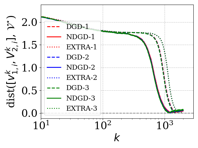
(b) Evolution of distance between (𝐯1,ik,𝐕2,ik)(\mathbf{v}_{1,i}^{k},\mathbf{V}_{2,i}^{k}) at agent ii and set 𝒱⋆\mathcal{V}^{\star} at agent 11 and 22.
Refer to caption
(c) Evolution of the consensus error at agent 11, where 𝐕^k=[(𝐯1,1k,𝐕2,1k]⊤\hat{\mathbf{V}}^{k}=[(\mathbf{v}_{1,1}^{k},\mathbf{V}_{2,1}^{k}]^{\top}, and 𝐕¯k=1m​∑i=1m[𝐯1,ik,𝐕2,ik]⊤\bar{\mathbf{V}}^{k}=\frac{1}{m}\sum_{i=1}^{m}[\mathbf{v}_{1,i}^{k},\mathbf{V}_{2,i}^{k}]^{\top}.
Refer to caption
(d) Mean distance between (𝐯1,1k,𝐕2,1k)(\mathbf{v}_{1,1}^{k},\mathbf{V}_{2,1}^{k}) and the set 𝒱⋆\mathcal{V}^{\star}, with 95% confidence intervals.
Figure 1: Second-order properties of NDGD and DGD for the binary classification example. The set of local minimizers of L~\tilde{L} is denoted by 𝒱⋆\mathcal{V}^{\star} and marked by red ⋆\star.

4 Numerical Examples

In this section, through one illustrative numerical example, we demonstrate how noise can help the distributed gradient descent algorithm efficiently escape saddle points and converge to the vicinity of local minimizers. Another non-convex quartic optimization example can be found in [21].

We then explore training a basic neural network for binary classification as a classic example of non-convex distributed optimization [4, 31]. Given a dataset (X,Y)(X,Y) where X={x(1),x(2),…,x(m)}X=\{x^{(1)},x^{(2)},\dots,x^{(m)}\} are the input features and Y={y(1),y(2),…,y(m)}Y=\{y^{(1)},y^{(2)},\dots,y^{(m)}\} are the corresponding binary class labels, where x(i)∈ℝnx^{(i)}\in\mathbb{R}^{n} and y(i)∈{0,1}y^{(i)}\in\{0,1\} for all i=1,…,mi=1,\dots,m. The neural network’s task is to learn the weights 𝐯1∈ℝd\mathbf{v}_{1}\in\mathbb{R}^{d}, 𝐕2∈ℝd×n\mathbf{V}_{2}\in\mathbb{R}^{d\times n} that minimize the binary cross-entropy loss:

L​(𝐯1,𝐕2)=−1m​∑i=1m[y(i)​ln⁡(y^(i))+(1−y(i))​ln⁡(1−y^(i))],\displaystyle L(\mathbf{v}_{1},\mathbf{V}_{2})=-\frac{1}{m}\sum_{i=1}^{m}\left[y^{(i)}\ln(\hat{y}^{(i)})+(1-y^{(i)})\ln(1-\hat{y}^{(i)})\right],

where y^(i)\hat{y}^{(i)} is the predicted probability for the ii-th input computed as a sigmoid activation function:

y^(i)=11+exp⁡(−𝐯1⊤​𝐕2​x(i)).\displaystyle\hat{y}^{(i)}=\frac{1}{1+\exp(-\mathbf{v}_{1}^{\top}\mathbf{V}_{2}x^{(i)})}.

This objective can be simplified as an equivalent logistic loss with regularization terms:

L​(𝐯1,𝐕2)=1m​∑i=1mln⁡(1+exp⁡(−y~(i)​𝐯1⊤​𝐕2​x(i))),\displaystyle L(\mathbf{v}_{1},\mathbf{V}_{2})=\frac{1}{m}\sum_{i=1}^{m}\ln(1+\exp(-\tilde{y}^{(i)}\mathbf{v}_{1}^{\top}\mathbf{V}_{2}x^{(i)})),

where for all i=1,…,mi=1,\dots,m,

y~(i)={−1,if​y(i)=0;1,if​y(i)=1.\displaystyle\tilde{y}^{(i)}=\begin{cases}-1,&\text{if}~y^{(i)}=0;\\ 1,&\text{if}~y^{(i)}=1.\end{cases}

Then, as an instance of Problem (1), the learning problem with regularization term can be formulated as

min𝐯1,𝐕2⁡L~​(𝐯1,𝐕2)=∑i=1mL~i​(𝐯1,𝐕2),\displaystyle\min_{\mathbf{v}_{1},\mathbf{V}_{2}}\tilde{L}(\mathbf{v}_{1},\mathbf{V}_{2})=\sum_{i=1}^{m}\tilde{L}_{i}(\mathbf{v}_{1},\mathbf{V}_{2}),

where

L~i​(𝐯1,𝐕2)=1m​ln⁡(1+exp⁡(−y~(i)​𝐯1⊤​𝐕2​x(i)))+η2​m​(‖𝐯1‖2+‖𝐕2‖F2).\tilde{L}_{i}(\mathbf{v}_{1},\mathbf{V}_{2})=\frac{1}{m}\ln(1+\exp(-\tilde{y}^{(i)}\mathbf{v}_{1}^{\top}\mathbf{V}_{2}x^{(i)}))\\ +\frac{\eta}{2m}(\|\mathbf{v}_{1}\|^{2}+\|\mathbf{V}_{2}\|_{F}^{2}).

For a straightforward visualization of the learning problem, we select parameters that render all variables as scalars, setting n=d=1n=d=1. Consider we engage m=50m=50 agents to collaboratively solve this problem, connecting them in a regular graph with a degree of 22. Note that each agent ii only knows its local objective L~i​(𝐯1,𝐕2)\tilde{L}_{i}(\mathbf{v}_{1},\mathbf{V}_{2}). By examining the Hessian at (0,0)(0,0), it follows that L~​(𝐯1,𝐕2)\tilde{L}(\mathbf{v}_{1},\mathbf{V}_{2}) has three critical points: two local minimizers and one saddle point, as illustrated in Fig. 1(a). The saddle point (marked by ×\times) is located at (0,0)(0,0), and the local minimizers (marked by ⋆\star) lie symmetrically in the positive and negative quadrants. We set η=0.1\eta=0.1, generate y~(i)\tilde{y}^{(i)} uniformly from {−1,1}\{-1,1\}, and x(i)∼𝒩​(y~(i),1)x^{(i)}\sim\mathcal{N}(\tilde{y}^{(i)},1). The algorithm parameters are α=0.9\alpha=0.9, σ=0.55\sigma=0.55, and K=2500K=2500. In Fig. 1(a), agents are initialized close to the stable manifold of the saddle point. DGD approaches the saddle, whereas both NDGD and EXTRA move toward a local minimizer. For clarity, only agent 11 is shown; additional agents are illustrated in subsequent figures. In Fig. 1(b), DGD requires about 600600 iterations to escape, while NDGD escapes within about 100100 iterations and converges to a neighborhood of a local minimizer. EXTRA also converges to a local minimizer, but more slowly than NDGD. Trajectories of three representative agents are included to illustrate distributed behavior. We also report the consensus error ‖𝐱^ik−av⁡(𝐱^k)‖\|\hat{\mathbf{x}}_{i}^{k}-\operatorname{av}(\hat{\mathbf{x}}^{k})\|, noting that the bound ζ\zeta is conservative and therefore omitted for clarity. Results are averaged over multiple trials with 95%95\% confidence intervals. EXTRA consistently achieves lower consensus error, suggesting a potential direction for future work that combines its strong consensus properties with stochastic perturbations. This example highlights the effectiveness of NDGD in escaping saddle points compared to DGD, while also showing competitive performance relative to EXTRA.

5 Conclusions and Discussion

This paper studied a noisy distributed gradient descent (NDGD) method for distributed non-convex optimization over networks. By introducing stochastic perturbations into the distributed updates, the proposed method enables saddle-point escape while preserving consensus and distributed implementation. Under suitable regularity conditions, high-probability convergence guarantees were established for all agents to a neighborhood of a common local minimizer, with explicit characterization of both optimality and consensus errors. Numerical experiments demonstrated improved saddle-point escape and solution quality compared with standard DGD and EXTRA. Future work will consider weaker geometric assumptions and extensions to more general distributed optimization settings.

References

References

  • [1] Y. Bo and Y. Wang (2024) Quantization avoids saddle points in distributed optimization. Proceedings of the National Academy of Sciences 121 (17), pp. e2319625121. Cited by: §1.2.
  • [2] S. Boyd, N. Parikh, E. Chu, B. Peleato, and J. Eckstein (2011) Distributed optimization and statistical learning via the alternating direction method of multipliers. Foundations and Trends in Machine Learning 3 (1), pp. 1–122. Cited by: §1.
  • [3] E. Camponogara and H. F. Scherer (2010) Distributed optimization for model predictive control of linear dynamic networks with control-input and output constraints. IEEE Transactions on Automation Science and Engineering 8 (1), pp. 233–242. Cited by: §1.
  • [4] A. Daneshmand, G. Scutari, and V. Kungurtsev (2020) Second-order guarantees of distributed gradient algorithms. SIAM Journal on Optimization 30 (4), pp. 3029–3068. Cited by: §1.2, §1.2, §2.2, §2.3, §4.
  • [5] P. Di Lorenzo and G. Scutari (2015) Distributed nonconvex optimization over networks. In Proc. IEEE Int. Workshop Computational Advances in Multi-Sensor Adaptive Processing (CAMSAP), pp. 229–232. Cited by: §1.2.
  • [6] P. Di Lorenzo and G. Scutari (2016) NEXT: in-network nonconvex optimization. IEEE Transactions on Signal and Information Processing over Networks 2 (2), pp. 120–136. Cited by: §1.2.
  • [7] S. S. Du, C. Jin, J. D. Lee, M. I. Jordan, A. Singh, and B. Póczos (2017) Gradient descent can take exponential time to escape saddle points. In Advances in Neural Information Processing Systems (NeurIPS), Vol. 30. Cited by: §1.2.
  • [8] R. Ge, F. Huang, C. Jin, and Y. Yuan (2015) Escaping from saddle points—online stochastic gradient for tensor decomposition. In Proc. Conf. Learning Theory (COLT), pp. 797–842. Cited by: §1.2.
  • [9] D. Jakovetić, J. Xavier, and J. M. F. Moura (2014) Fast distributed gradient methods. IEEE Transactions on Automatic Control 59 (5), pp. 1131–1146. Cited by: §1.2.
  • [10] C. Jin, R. Ge, P. Netrapalli, S. M. Kakade, and M. I. Jordan (2017) How to escape saddle points efficiently. In Proc. Int. Conf. Machine Learning (ICML), pp. 1724–1732. Cited by: §1.2.
  • [11] C. Jin, P. Netrapalli, R. Ge, S. M. Kakade, and M. I. Jordan (2021) On nonconvex optimization for machine learning: gradients, stochasticity, and saddle points. Journal of the ACM 68 (2), pp. 1–29. Cited by: §1.2.
  • [12] B. Johansson, M. Rabi, and M. Johansson (2007) A simple peer-to-peer algorithm for distributed optimization in sensor networks. In Proc. IEEE Conf. Decision and Control (CDC), pp. 4705–4710. Cited by: §1.
  • [13] J. Konečnỳ, B. McMahan, and D. Ramage (2015) Federated optimization: distributed optimization beyond the datacenter. arXiv preprint arXiv:1511.03575. Cited by: §1.
  • [14] B. McMahan, E. Moore, D. Ramage, S. Hampson, and B. A. y Arcas (2017) Communication-efficient learning of deep networks from decentralized data. In Proc. Int. Conf. Artificial Intelligence and Statistics (AISTATS), pp. 1273–1282. Cited by: §1.
  • [15] D. K. Molzahn, F. Dörfler, H. Sandberg, S. H. Low, S. Chakrabarti, R. Baldick, and J. Lavaei (2017) A survey of distributed optimization and control algorithms for electric power systems. IEEE Transactions on Smart Grid 8 (6), pp. 2941–2962. Cited by: §1.
  • [16] A. Nedić and J. Liu (2018) Distributed optimization for control. Annual Review of Control, Robotics, and Autonomous Systems 1, pp. 77–103. Cited by: §1.
  • [17] A. Nedic, A. Olshevsky, and W. Shi (2017) Achieving geometric convergence for distributed optimization over time-varying graphs. SIAM Journal on Optimization 27 (4), pp. 2597–2633. Cited by: §1.2.
  • [18] A. Nedic, A. Ozdaglar, and P. A. Parrilo (2010) Constrained consensus and optimization in multi-agent networks. IEEE Transactions on Automatic Control 55 (4), pp. 922–938. Cited by: §1.2.
  • [19] A. Nedic and A. Ozdaglar (2009) Distributed subgradient methods for multi-agent optimization. IEEE Transactions on Automatic Control 54 (1), pp. 48–61. Cited by: §1.2, §1, §2.2.
  • [20] L. Qin, M. Cantoni, and Y. Pu (2023) Second-order properties of noisy distributed gradient descent. In Proc. IEEE Conf. Decision and Control (CDC), pp. 7324–7329. Cited by: §1.2, §1.
  • [21] L. Qin, M. Cantoni, and Y. Pu (2025) Convergence analysis of noisy distributed gradient descent for non-convex optimization—saddle point escape. arXiv preprint arXiv:2510.20246. Cited by: §1.2, §2.2, §2, §3, §3, §4.
  • [22] G. Qu and N. Li (2017) Harnessing smoothness to accelerate distributed optimization. IEEE Transactions on Control of Network Systems 5 (3), pp. 1245–1260. Cited by: §1.2.
  • [23] M. Rabbat and R. Nowak (2004) Distributed optimization in sensor networks. In Proc. 3rd Int. Symp. Information Processing in Sensor Networks (IPSN), pp. 20–27. Cited by: §1.
  • [24] W. Shi, Q. Ling, G. Wu, and W. Yin (2015) EXTRA: an exact first-order algorithm for decentralized consensus optimization. SIAM Journal on Optimization 25 (2), pp. 944–966. Cited by: §1.2.
  • [25] B. Swenson, S. Kar, H. V. Poor, and J. M. F. Moura (2019) Annealing for distributed global optimization. In Proc. IEEE Conf. Decision and Control (CDC), pp. 3018–3025. Cited by: Remark 2.
  • [26] B. Swenson, R. Murray, H. V. Poor, and S. Kar (2019) Distributed gradient descent: nonconvergence to saddle points and the stable-manifold theorem. In Proc. Allerton Conf. Communication, Control, and Computing, pp. 595–601. Cited by: §1.2.
  • [27] B. Swenson, R. Murray, H. V. Poor, and S. Kar (2022) Distributed stochastic gradient descent: nonconvexity, nonsmoothness, and convergence to local minima. Journal of Machine Learning Research 23 (1), pp. 14751–14812. Cited by: §1.2.
  • [28] H. Terelius, U. Topcu, and R. M. Murray (2011) Decentralized multi-agent optimization via dual decomposition. IFAC Proceedings Volumes 44 (1), pp. 11245–11251. Cited by: §1.2.
  • [29] K. I. Tsianos and M. G. Rabbat (2012) Distributed strongly convex optimization. In Proc. Allerton Conf. Communication, Control, and Computing, pp. 593–600. Cited by: §1.2.
  • [30] S. Vlaski and A. H. Sayed (2021) Distributed learning in non-convex environments—part i: agreement at a linear rate. IEEE Transactions on Signal Processing 69, pp. 1242–1256. Cited by: §1.2, Remark 2.
  • [31] S. Vlaski and A. H. Sayed (2021) Distributed learning in non-convex environments—part ii: polynomial escape from saddle points. IEEE Transactions on Signal Processing 69, pp. 1257–1270. Cited by: §1.2, §4.
  • [32] Y. Wang and T. Başar (2023) Decentralized nonconvex optimization with guaranteed privacy and accuracy. Automatica 150, pp. 110858. Cited by: §1.2.
  • [33] X. Yi, S. Zhang, T. Yang, T. Chai, and K. H. Johansson (2022) A primal-dual sgd algorithm for distributed nonconvex optimization. IEEE/CAA Journal of Automatica Sinica 9 (5), pp. 812–833. Cited by: §1.2.
  • [34] K. Yuan, Q. Ling, and W. Yin (2016) On the convergence of decentralized gradient descent. SIAM Journal on Optimization 26 (3), pp. 1835–1854. Cited by: §1.2, §1.2, §2.2.
  • [35] J. Zeng and W. Yin (2018) On nonconvex decentralized gradient descent. IEEE Transactions on Signal Processing 66 (11), pp. 2834–2848. Cited by: §1.2, §1.2, §2.2, §2.2.