Unsupervised Deep Generative Models for Anomaly Detection in Neuroimaging: A Systematic Scoping Review

Youwan Mahé ^1,2∗ Elise Bannier^1,3 Stéphanie Leplaideur^1,4,5
Elisa Fromont^6§ and Francesca Galassi ^1∗§
¹Univ Rennes, Inria, CNRS, Inserm, IRISA UMR 6074, Empenn, Rennes, France,
²Siemens Healthineers, Courbevoie, France
³CHU Rennes, Radiology Department, Rennes, France
⁴CHU Rennes, Physical Medicine and Rehabilitation Department, Rennes, France
⁵Centre de Kerpape, Ploemeur, France
⁶Univ Rennes, Inria, CNRS, IRISA, Rennes, France
^§ These authors contributed equally as co–last authors.
^∗Correspondence: [youwan.mahe, francesca.galassi]@inria.fr

Abstract

Unsupervised anomaly detection (UAD) based on deep generative modelling has been increasingly explored for identifying pathological brain abnormalities without requiring voxel-level annotations. By learning the distribution of healthy anatomy and generating pseudo-healthy reconstructions, these methods aim to localise deviations in a pathology-agnostic manner. Despite rapid methodological development - from autoencoders and variational autoencoders to generative adversarial networks and diffusion-based models - a structured synthesis of their application in structural neuroimaging is lacking.

We conducted a PRISMA-ScR–guided scoping review of studies published between January 2018 and December 2025 that applied unsupervised deep generative models to anomaly detection in brain MRI (and, less frequently, CT). Thirty-three studies met inclusion criteria. Methods were categorised by architectural family, and reported performance was synthesised across major pathology groups, with segmentation (Dice) and detection metrics (AUROC, AUPRC) disaggregated by evaluation level (voxel, slice, subject). For transparency, we also summarised dataset characteristics, dimensionality (2D vs. 3D), and thresholding strategies.

Reported performance varied substantially across studies and pathologies. Dice scores generally ranged from approximately 0.30 to 0.75, while voxel-level AUROC values spanned roughly 0.58 to 0.97. Performance was typically higher for large focal lesions, such as brain tumours, than for small or diffuse abnormalities including white-matter hyperintensities. Across overlapping performance ranges, no architectural family consistently dominated across pathologies. Reported metrics were strongly influenced by evaluation level, thresholding strategy, and dataset composition, limiting direct cross-study comparability.

Overall, unsupervised generative approaches demonstrate potential for pathology-agnostic anomaly localisation, particularly in settings where annotated data are scarce. However, methodological heterogeneity, limited external validation, and sensitivity to dataset characteristics remain important challenges. Emerging paradigms - including anatomy-aware modelling, diffusion-based frameworks, and alternative normative evaluation metrics - seek to address these limitations and improve robustness and clinical relevance.

Keywords: Unsupervised Anomaly Detection (UAD), Deep Generative Modelling, Neuroimaging, Magnetic Resonance Imaging (MRI)

1 Introduction

Brain magnetic resonance imaging (MRI) plays a central role in the diagnosis, monitoring, and prognosis of neurological disease. Structural MRI enables high-resolution in vivo visualisation of abnormalities such as tumours, vascular infarcts, white-matter hyperintensities, demyelinating lesions, traumatic injury, and regional atrophy [Crimi2021]. Their appearance varies substantially across imaging sequences and pathology types [Vemuri2022, VillanuevaMeyer2017], complicating reliable delineation. Accurate segmentation is essential for deriving quantitative biomarkers - including lesion load, spatial distribution, and longitudinal volumetric change - that support clinical decision-making and research studies. However, manual detection and segmentation by expert radiologists remain time-consuming, require specialised expertise, and are subject to inter- and intra-rater variability [Darrault2025, walsh2023expert]. The development of robust automated tools is therefore a major priority.

Before the rise of deep learning, automated lesion detection relied on classical image-processing and statistical modelling approaches, including Gaussian mixture models, fuzzy c-means clustering, and Markov random fields [Gonzalez2007, GarciaLorenzo2013]. While effective in controlled settings, these techniques required expert-defined features and were sensitive to anatomical variability and acquisition differences [Xu2024]. The advent of deep learning transformed medical image analysis by enabling multi-scale feature learning directly from data [Litjens2017]. In neuroimaging, convolutional architectures such as U-Net [Ronneberger2015] and its derivatives, including nnU-Net [Isensee2024], have achieved state-of-the-art performance on curated benchmarks. Large public datasets such as BraTS for brain tumours [Menze2015] and MSSEG for multiple sclerosis [Commowick2021] have facilitated this progress.

Despite these advances, supervised models exhibit important limitations. Their performance depends critically on large voxel-level annotated datasets, which are costly to produce and often unavailable in rare or heterogeneous diseases [Lee2022]. Moreover, supervised approaches operate under a closed-set assumption: they are trained to recognise predefined lesion categories and may struggle under distribution shift caused by variations in pathology subtype, patient population, or acquisition protocol [Ghafoorian2017]. As a result, accuracy may deteriorate substantially outside curated benchmarks.

Unsupervised anomaly detection (UAD) offers a complementary paradigm. Rather than learning to segment predefined abnormalities, UAD methods aim to model the distribution of healthy anatomy and detect deviations from this normative representation. In neuroimaging, this is typically achieved by training generative models exclusively on healthy brain scans. At inference, a pathological image is mapped toward a pseudo-healthy reconstruction, and spatial discrepancies between the input and its reconstruction highlight candidate abnormalities. This reconstruction-based strategy enables pathology-agnostic detection and may be particularly valuable in settings where annotations are scarce, diseases are rare, or lesion phenotypes are heterogeneous. Recent open-set evaluations, such as the NOVA benchmark [Bercea2025-2], have demonstrated substantial performance drops for state-of-the-art models on rare and heterogeneous pathologies, underscoring the need for distribution-modelling approaches that do not rely on predefined lesion categories.

Over the past decade, deep generative modelling has evolved rapidly. Early work employed autoencoders and variational autoencoders (VAEs) to learn compact representations of healthy anatomy [Zimmerer2019]. Generative adversarial networks (GANs) were subsequently introduced to improve reconstruction realism and boundary sharpness [Schlegl2019]. More recently, denoising diffusion probabilistic models (DDPMs) [Ho2020] and related continuous-time generative frameworks have demonstrated strong capacity for modelling complex anatomical variability and producing high-fidelity pseudo-healthy reconstructions [Pinaya2022-3, Bercea2023]. These methodological advances have expanded the landscape of unsupervised neuroimaging anomaly detection.

Several reviews have addressed subsets of this literature, including autoencoder and diffusion-based anomaly detection [Baur2021-1, BerceaReview2025], GAN applications in medical imaging [Wang2023], and broader surveys of generative models in healthcare [Pang2021, Tschuchnig2022]. However, to our knowledge, no prior review has systematically synthesised unsupervised deep generative models for structural neuroimaging from a pathology-stratified perspective while explicitly disaggregating segmentation and detection metrics, evaluation levels (voxel, slice, subject), thresholding strategies, and dataset characteristics. Reported performance varies substantially depending on lesion type, evaluation protocol, and data composition, complicating cross-study comparison and interpretation.

In this PRISMA-ScR–guided scoping review, we systematically analyse unsupervised deep generative models for anomaly detection in structural neuroimaging published between 2018 and December 2025. We categorise methods into four principal architectural families - autoencoders, variational autoencoders, generative adversarial networks, and diffusion-based models - and synthesise their performance across major pathology groups, including brain tumours, stroke, multiple sclerosis, and white-matter hyperintensities. Beyond architectural comparison, we examine the influence of dimensionality (2D vs. 3D), dataset composition, thresholding strategies, and evaluation level on reported metrics. Finally, we discuss methodological limitations of reconstruction-based approaches and highlight emerging paradigms aimed at improving robustness, interpretability, and clinical relevance.

1.1 Review questions

This scoping review addresses the following questions:

(i)

Which unsupervised deep generative model families (AE, VAE, GAN, diffusion/flow) have been applied to anomaly detection and/or segmentation in structural neuroimaging since 2018?
(ii)

How are these methods evaluated (evaluation level, metrics, and thresholding strategy), and how do reported results vary across major pathology groups?
(iii)

What methodological design variations (e.g., 2D vs. 3D processing, patching or masking strategies, pretraining) are described in the literature, and how are they reported in relation to performance?
(iv)

What emerging paradigms aim to address current limitations of reconstruction-based anomaly detection?

2 Methods

2.1 Background: generative modelling for unsupervised anomaly detection

Generative models aim to learn the distribution of healthy brain images, thereby capturing normative anatomical variability. When an explicit probabilistic formulation is available, this can be written as approximating the data distribution $p_{\text{data}}(\mathbf{x})$ with a distribution $p_{\theta}(\mathbf{x})$ induced by a parameterised mapping. In neuroimaging UAD, models are trained on healthy brain images only, so the learned distribution represents normative anatomy rather than pathology.

Many generative approaches introduce a latent variable $\mathbf{z}\in\mathbb{R}^{d}$ , drawn from a simple prior distribution $p(\mathbf{z})$ , typically a standard multivariate Gaussian $\mathcal{N}(\mathbf{0},\mathbf{I})$ , and a neural network $G_{\theta}$ that maps latent codes to image space:

\mathbf{z}\sim p(\mathbf{z})=\mathcal{N}(\mathbf{0},\mathbf{I}),\qquad\mathbf{x}=G_{\theta}(\mathbf{z}),\qquad\mathbf{x}\sim p_{\theta}(\mathbf{x}).

(1)

When an explicit encoder $E_{\phi}$ is available (e.g., autoencoders and VAEs), a test image $\mathbf{x}_{\text{test}}$ is mapped to latent space as

\mathbf{z}=E_{\phi}(\mathbf{x}_{\text{test}}),\qquad\hat{\mathbf{x}}=G_{\theta}(\mathbf{z}).

(2)

For models without an encoder (e.g., classical GANs or some diffusion-based methods), a latent representation must instead be obtained through an inversion or optimisation procedure:

\mathbf{z}^{\ast}=\arg\min_{\mathbf{z}}\;\mathrm{dist}\big(\mathbf{x}_{\text{test}},G_{\theta}(\mathbf{z})\big),\qquad\hat{\mathbf{x}}=G_{\theta}(\mathbf{z}^{\ast}),

(3)

where $\mathrm{dist}(\cdot,\cdot)$ denotes a similarity or dissimilarity measure (e.g., $\ell_{1}$ , $\ell_{2}$ , SSIM).

Because pathological patterns are absent from the healthy training distribution, they are typically not faithfully reconstructed in the pseudo-healthy image $\hat{\mathbf{x}}$ . An anomaly map is therefore defined as

\mathbf{r}=\mathrm{dist}\big(\mathbf{x}_{\text{test}},\hat{\mathbf{x}}\big),

(4)

highlighting spatial deviations from normative anatomy without requiring voxel-level annotations.

Despite substantial architectural differences between autoencoders, variational autoencoders, generative adversarial networks, and diffusion models, this reconstruction-based principle underpins the majority of unsupervised generative approaches reviewed in this work. Subsequent sections compare how different architectures, dimensionalities, and training strategies affect the quality of pseudo-healthy reconstructions and the reliability of the resulting anomaly maps.

2.2 Information sources and search strategy

This review was conducted in accordance with the PRISMA-ScR (2018) guidelines for scoping reviews [Tricco2018]. We searched PubMed, Web of Science, ScienceDirect, Springer Link, IEEE Xplore, and ArXiv up to 17 December 2025, including early-access preprints. Boolean queries combined terms related to unsupervised anomaly detection, neuroimaging (MRI or CT), and deep learning, as summarised in Table 1. Reference lists of relevant articles and reviews were also screened. Searches were limited to articles published in English.

Table 1: Boolean queries used for database searching

Database	Query	Date
PubMed	(Anomaly AND Unsupervised) AND Brain) AND (MRI OR CT) AND (Machine Learning OR Deep Learning)	Dec 17 2025
Web Of Science	((TS=Anomaly) AND (TS=unsupervised) AND (TS=brain)) AND ((TS=MRI) OR (TS=CT)) AND ((TS=Machine Learning) OR (TS=Deep Learning))	Dec 17 2025
Science Direct	Unsupervised Anomaly Brain MRI CT Machine Learning Filter : Research Article	Dec 17 2025
ArXiv	Unsupervised AND Anomaly AND Brain AND ”Deep learning”, in Computer Science (cs)	Dec 17 2025
IEEE Xplore	Unsupervised AND Anomaly AND Brain AND ”Deep Learning”	Dec 17 2025
Springer Nature Link	(Anomaly AND Unsupervised AND Brain) AND (MRI OR CT) AND (Machine Learning OR Deep Learning) AND (”Conference Paper” OR ”Research Article”) AND (”Computer Vision” OR ”Machine Learning”)	Dec 17 2025

2.3 Eligibility and screening

Studies were eligible if they:

•

proposed or evaluated an unsupervised deep learning method for anomaly detection and/or lesion segmentation in structural neuroimaging (MRI or CT), trained exclusively on healthy data to model normative anatomy (i.e., without access to pathological labels);
•

reported at least one quantitative evaluation metric relevant to detection (e.g., AUROC, AUPRC) or segmentation (e.g., Dice);
•

used real human imaging data from public datasets or institutional cohorts.

Unsupervised learning can be characterised in multiple ways. A narrow definition restricts it to methods that lack any explicit label-driven training objective, thereby excluding self-supervised approaches [Dosovitskiy2014]. In this review, we adopt a pragmatic definition aligned with anomaly detection in medical imaging: we include methods trained without using real pathological labels (neither voxel-level segmentations nor subject-/case-level diagnostic labels) in the training objective. This encompasses approaches that use proxy or self-supervised objectives to model the distribution of healthy data (e.g., masked autoencoding, lesion synthesis, or discriminative proxy tasks) [Goodfellow2016]. In Table LABEL:tab:method_summary, methods employing such proxy or self-supervised objectives are denoted with a ^P.

We excluded studies that employed rule-based or non-deep learning approaches; fully supervised or semi-supervised methods requiring pathological annotations; non-generative methods (except where discussed contextually); non-neuroimaging applications; animal-only or synthetic-only data; review papers; and non-research formats (e.g., abstracts, editorials). For transparency, self-supervised non-generative and hybrid approaches are discussed in a separate contextual subsection but are not included in the main quantitative synthesis because they do not satisfy the generative modelling inclusion criteria. Although some applications use deep generative models for functional or diffusion imaging (e.g., FDG-PET, diffusion tensor imaging, or functional MRI) [Hassanaly2024-ex, Solal2023-ex, Muñoz-Ramírez2022-ex, Sathyanarayanan2025-ex], we restricted the primary synthesis to structural imaging to ensure comparability across studies. Similarly, we excluded studies that did not report voxel-, slice-, or subject-level quantitative performance metrics.

Search results were imported into Rayyan [Ouzzani2016] for duplicate removal and blinded screening by two reviewers. Titles and abstracts were screened first, followed by full-text assessment of potentially relevant studies. Disagreements were resolved through discussion until consensus was reached.

Bibliographic records were retrieved using the export functions of each database (CSV or BibTeX) and imported into Rayyan for record matching and management. For arXiv, where no export function is available through the web interface, we used the API via custom Python scripts to obtain publication metadata. Full-text articles were accessed through institutional subscriptions where available.

Data extraction was performed independently by two reviewers using a structured extraction form developed for this review. Extracted variables included: publication year, model architecture, imaging modality, dimensionality (2D or 3D), training and test datasets, pathology type, evaluation level (voxel, slice, or subject), thresholding strategy, and reported quantitative performance metrics (Dice, AUROC, AUPRC). Extracted data were tabulated and used for qualitative and quantitative synthesis.

2.4 Risk of bias assessment

Risk of bias was assessed with a focus on methodological quality. Guided by PRISMA recommendations for systematic reviews [Page2021], two reviewers (YM, FG) independently screened and appraised all records in Rayyan using blind mode. Disagreements were resolved by discussion until consensus. As no validated risk-of-bias tool exists for anomaly detection in medical imaging, we applied a structured checklist covering dataset characteristics (e.g., public availability, diversity of pathologies), as well as reproducibility and transparency (e.g., code and data availability). For studies raising concerns about reporting integrity, we additionally screened them with the Problematic Paper Screener [Cabanac2022] and documented outcomes.

3 Results

3.1 Study selection

The initial search identified 574 records. After duplicate removal and title/abstract screening, 527 records were excluded according to predefined eligibility criteria (e.g., out of scope, non-neuroimaging, non-deep learning, rule-based methods, review articles). Forty-seven full-text articles were assessed for eligibility, of which 14 were excluded (e.g., absence of structural imaging, lack of quantitative metrics, non-research format). A total of 33 studies were included in the final synthesis (Fig. 1). The included studies were published between January 2018 and 17 December 2025 (including early-access articles), providing an eight-year overview of unsupervised deep generative models applied to structural neuroimaging.

Refer to caption — Figure 1: PRISMA flow diagram for scoping reviews, including database and register searches.

3.2 Study characteristics

Across the 33 included studies, four main architectural families were identified: autoencoders (AEs), variational autoencoders (VAEs), generative adversarial networks (GANs), and diffusion-based models. Although standard AEs do not explicitly define a probabilistic generative model, they are widely used as reconstruction-based normative baselines and are therefore included in this synthesis. Proxy or self-supervised pretext objectives were included when used to support pseudo-healthy reconstruction (e.g., masking/inpainting or structured corruption). In total, the 33 studies comprised 9 autoencoder-based approaches, 9 variational autoencoders, 4 GAN-based methods, and 11 diffusion-based models.

MRI constituted the primary imaging modality (T1-w, T1-w Gd, T2-w, and FLAIR), with occasional use of computed tomography. Most methods processed 2D slices, although an increasing subset employed volumetric 3D architectures, particularly among recent AE/VAE studies and selected GAN and diffusion approaches. Although some generative models have been applied to non-structural modalities such as FDG-PET for Alzheimer’s disease detection [Hassanaly2024-ex, Solal2023-ex], this review focused on structural imaging to ensure methodological comparability across studies.

3.3 Evaluation metrics

Most studies reported either segmentation or detection performance. Segmentation accuracy was assessed using the Dice similarity coefficient (DSC or Dice score), defined as

\text{DSC}=\frac{2|X\cap Y|}{|X|+|Y|},

(5)

where $X$ is the predicted segmentation and $Y$ the reference annotation. Dice scores depend not only on the quality of the anomaly map but also on the thresholding strategy used to binarise residual maps. Threshold selection varied substantially across studies. In several cases, thresholds were retrospectively chosen to maximise Dice on the test set, yielding optimistic upper-bound estimates that may not reflect clinically deployable performance. Dice is also sensitive to lesion size and can disproportionately penalise small or sparse abnormalities. Detection was formulated as a binary classification problem (pathological vs. non-pathological) and quantified using AUROC and AUPRC. In highly imbalanced voxel-level tasks, AUPRC is often more informative than AUROC because it better reflects precision under class imbalance. Detection metrics were computed at different evaluation levels (voxel/pixel, slice, subject). Because these correspond to distinct classification tasks, values are not directly comparable across evaluation regimes.

Comparability across studies. Substantial heterogeneity exists in dataset composition, preprocessing pipelines, anomaly-map post-processing, thresholding strategies, and evaluation levels. Accordingly, reported performance values should be interpreted as descriptive indicators within each experimental setting rather than direct head-to-head comparisons across architectures.

3.4 Datasets and pathologies

Performance metrics were reported across a range of publicly available and institutional neuroimaging datasets. Three pathology groups predominated in the literature: brain tumours, multiple sclerosis (MS)/white-matter hyperintensities (WMH), and stroke. Fewer studies addressed neurodegenerative conditions (e.g., Alzheimer’s disease, Parkinson’s disease), traumatic brain injury, neonatal encephalopathy, or healthy ageing. Representative examples of central axial slices from the principal pathological datasets are shown in Figure 2. A structured overview of dataset characteristics - including cohort size, imaging modality, and documented biases - is provided in Table LABEL:tab:dataset_summary. Because dataset composition, acquisition protocols, and pathology prevalence vary substantially across studies, these factors should be considered when interpreting reported performance metrics.

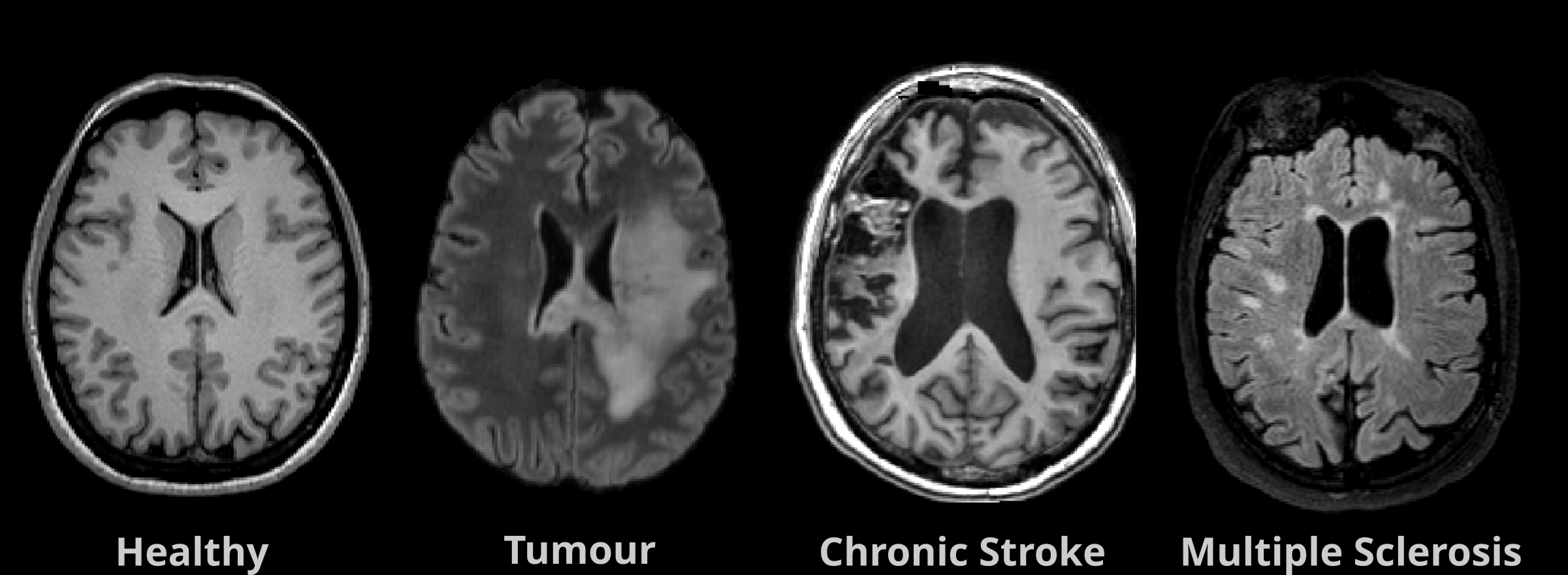
Brain tumours.

The majority of tumour studies relied on the Brain Tumor Segmentation (BraTS) challenge datasets [Menze2015], which provide multi-sequence MRI including T1-weighted (T1-w), contrast-enhanced T1-w (T1-w Gd), T2-weighted (T2-w), and FLAIR images. As detailed in Table LABEL:tab:dataset_summary, BraTS has expanded substantially across releases: BraTS 2012 included 50 cases, BraTS 2015 increased to 253 cases (with a strong high-grade glioma predominance), BraTS 2017-2020 ranged from 477 to 660 cases with expert-revised annotations across multiple centres, and the most recent BraTS 2021-2023 (GLI) editions comprise approximately 2,040 multi-institutional cases [Baid2021]. A smaller number of studies used alternative cohorts, including the neuroimaging dataset of brain tumour patients from [Pernet2016] (22 cases) and the Brain Tumor Dataset (BTD) from [Cheng2017] (233 cases), which are comparatively smaller and more homogeneous than BraTS. Gliomas, the primary pathology represented in these datasets, typically produce large focal lesions with substantial mass effect. Lesion morphology varies according to tumour grade, and progressive growth within the cranial cavity frequently distorts surrounding anatomical structures. Sequence selection is clinically motivated: T2-w and FLAIR emphasise water content and oedema, whereas T1-w Gd highlights blood-brain barrier disruption through contrast enhancement [Menze2015].

Stroke.

Stroke lesions were primarily represented by the Ischaemic Stroke Lesion Segmentation (ISLES) 2015 dataset and the Anatomical Tracings of Lesions After Stroke (ATLAS) datasets (versions 1.1/1.2 and 2.0) [HernandezPetzsche2022, Liew2021], as summarised in Table LABEL:tab:dataset_summary. ISLES 2015 comprises two subsets: the Sub-acute Ischemic Stroke Lesion Segmentation (SISS) cohort (64 subjects imaged with T1-w, T2-w, FLAIR, and DWI) and the Stroke Perfusion Estimation (SPES) cohort (50 subjects imaged with T1-w, T2-w, DWI, and perfusion modalities). These cohorts target acute and sub-acute ischaemic stroke, where diffusion-weighted imaging (DWI) is most sensitive to early infarction. As stroke progresses, diffusion signal characteristics evolve and lesion conspicuity may decrease, making delineation on structural sequences such as FLAIR more challenging [HernandezPetzsche2022]. ATLAS v1.1/1.2 includes 229-304 chronic stroke cases acquired as T1-weighted MRI, while ATLAS v2.0 comprises 955 manually segmented T1-w MRI cases collected from 33 cohorts worldwide [Liew2021]. A key limitation of ATLAS is its reliance on T1-w imaging alone, where chronic infarcts often resemble cerebrospinal fluid and are accompanied by tissue loss and structural deformation. Overall, lesion stage (acute vs. chronic), available contrasts (multi-sequence vs. T1-w only), and lesion appearance vary substantially across datasets; consequently, reported anomaly detection and segmentation performance is heterogeneous and not directly comparable across studies.

Multiple sclerosis and white-matter hyperintensities.

Although multiple sclerosis (MS) and white-matter hyperintensities (WMH) arise from distinct pathological processes, they are described jointly here because they share similar imaging characteristics relevant to anomaly detection: small, sparse, FLAIR-hyperintense white-matter lesions with low lesion-to-brain volume ratios. As summarised in Table LABEL:tab:dataset_summary, MS was primarily evaluated using the ISBI 2015 Longitudinal MS Lesion Segmentation dataset (ISBI 2015) [Carass2017], the Multiple Sclerosis Segmentation dataset (MSSEG) [Commowick2018, Commowick2021], and the MSLUB dataset [Lesjak2017]. MSSEG (MICCAI 2016) comprises 53 subjects with four MRI contrasts (T1-w, T1-w Gd, proton density, and FLAIR), while ISBI 2015 includes 82 cases and is subject to mono-site bias. MSLUB is a smaller mono-site cohort of 30 subjects with T2-w, FLAIR, and proton density imaging. WMH were primarily evaluated using the WMH Segmentation Challenge dataset (WMH 2017; 170 subjects; T1-w and FLAIR), which is enriched for older participants and spans multiple scanners, introducing age- and scanner-related heterogeneity [Kuijf2022]. Unlike tumours or many stroke lesions, MS plaques and WMH are typically small, sparse, and spatially distributed. They are most conspicuous on FLAIR and T2-w MRI, where they appear as focal white-matter hyperintensities. These properties contribute to substantial variability in segmentation and anomaly detection performance across studies and remain a major bottleneck for reconstruction-based methods.

Traumatic brain injury.

Traumatic brain injury (TBI) was represented primarily by the CENTER-TBI cohort (Table LABEL:tab:dataset_summary), a large multicentre European dataset comprising $\sim$ 4,500 subjects, with imaging dominated by computed tomography (CT) [Steyerberg2019]. On CT, acute TBI may present as focal hyperdense haemorrhagic lesions (e.g., epidural or subdural haematomas) as well as smaller haemorrhagic foci; however, diffuse axonal injury is often subtle or not directly visible on standard CT, which can limit sensitivity for detecting microscopic injury patterns [Currie2015].

Neurodegeneration and other conditions.

A smaller subset of included studies leveraged neurodegenerative cohorts, most often through the Alzheimer’s Disease Neuroimaging Initiative (ADNI) [Beckett2015] and the Open Access Series of Imaging Studies (OASIS-3) [LaMontagne2019], as summarised in Table LABEL:tab:dataset_summary. ADNI is a large multi-phase public repository including structural MRI and PET imaging from cognitively normal individuals, subjects with mild cognitive impairment, and patients with Alzheimer’s disease ( $>2{,}000$ participants across phases). OASIS-3 is a longitudinal, single-site cohort comprising 1,098 participants (605 cognitively normal and 493 at-risk or demented individuals), with multi-contrast MRI including T1-w, T2-w, FLAIR, DWI, SWI, ASL, and resting-state fMRI.

Healthy control datasets.

Across studies, normative training data were sourced either from dedicated healthy cohorts (e.g., IXI, UK Biobank, HCP) or from healthy subsets extracted from mixed pathology datasets (denoted H in Table LABEL:tab:method_summary). A smaller number of studies relied on in-house institutional cohorts. Explicit reporting of screening procedures and contamination control was inconsistent. Frequently used resources included the IXI dataset¹¹1http://brain-development.org/ixi-dataset/ (approximately 600 healthy volunteers scanned across three London hospitals; T1-w, T2-w, and proton density MRI), which was widely employed for training autoencoder, VAE, and diffusion models. Large population-based cohorts were also used, including the UK Biobank (UKB), which provides multi-modal MRI for over 50,000 participants, and the Human Connectome Project (HCP; Young Adult cohort, N $\sim$ 1,200; ages 22–35 years) [VanEssen2012]. While UKB offers unprecedented scale, it is subject to healthy volunteer and geographical biases [Littlejohns2020]. HCP, although high-quality, reflects a restricted young adult demographic. Smaller normative datasets included the Cambridge Centre for Ageing and Neuroscience (Cam-CAN; N $\sim$ 650) [Shafto2014], the Neurofeedback Skull-stripped (NFBS) dataset (125 T1-w scans) [Puccio2016], and institutional in-house cohorts. A single diffusion-based study used a healthy subset of the FastMRI+ dataset (1,001 axial brain MRI scans) [Zhao2022]. The Medical Out-of-Distribution (MOOD) challenge [Zimmerer2020] dataset was used once. Notably, MOOD relies on synthetic anomalies injected into healthy HCP scans, which may introduce synthetic bias and inflate detection performance relative to real-world pathology. Although ADNI and OASIS-3 contain both healthy and pathological subjects, in the reviewed literature, they were primarily used as sources of cognitively normal control scans for training normative models rather than as primary anomaly detection benchmarks. It is important to note that ADNI controls exhibit a documented healthy volunteer bias [Gianattasio2021], and OASIS-3 reflects single-site demographic characteristics, which may influence normative modelling. A single study reported combining smaller healthy subsets of the individual brain charting (IBC), a high-resolution fMRI dataset for cognitive mapping [IBC2018], and from a multi-parametric neuroimaging reproducibility study referred here to as Kirby [Landman2011]

3.5 Synthesis by architecture

To provide a structured overview, we synthesised findings by architectural family and pathology. For segmentation tasks, we report Dice similarity coefficient (Dice) scores; for detection tasks, we report AUROC and AUPRC, always specifying the evaluation level (voxel/pixel, slice, or subject) to avoid misleading cross-study comparisons. Study characteristics and experimental setups are summarised in four complementary tables. Table LABEL:tab:dataset_summary describes datasets (release, size, modality, population, and known biases). Table LABEL:tab:method_summary summarises methods (architectural family, training/test datasets, imaging modality, and input dimensionality/processing strategy). Quantitative results are reported in Table LABEL:tab:detection_metrics for detection and Table LABEL:tab:dice_summary for segmentation.

Table 2: Comprehensive overview of neuroimaging datasets and their characteristics.

Dataset (Release)	Modality	Pathology	Population	Cases (N)	Known Biases & Characteristics
Tumour
BraTS ’12	MRI (4 seqs)	Glioma	Adult	50	Small sample size.
BraTS ’15	MRI (4 seqs)	Glioma	Adult	253	Skewed to HGG.
BraTS ’17-20	MRI (4 seqs)	Glioma	Adult	477-660	Expert-revised labels; pre-operative scan bias, n=19 centres.
BraTS ’21-23(GLI)	MRI (4 seqs)	Glioma	Adult	2,040	pre-operative scan bias; multi-site diversity.
[Pernet2016]	MRI (3 seqs)	Tumor	Adult	22	Small sample size,pre-operative.
[Cheng2017] (BTD)	MRI (T1w)	Tumor	Adult	233	Monocentric; private.
Stroke
ISLES 2015 (SISS)	MRI (4 seqs)	Sub-acute isch. Stroke	Adult	64	Mostly monocentric; ischemic stroke bias.
ISLES 2015 (SPES)	MRI (4 seqs)	acute isch. Stroke	Adult	50	monocentric; ischemic stroke bias.
ATLAS v1.1/1.2	MRI (T1w)	Chronic Stroke	Adult	229-304	Modality bias (T1w only), multicentric.
ATLAS v2.0	MRI (T1w)	Chronic Stroke	Adult	955	Modality bias (T1w only), multicentric.
Multiple Sclerosis (MS) and White Matter Hyperintensities (WMH)
ISBI 2015	MRI (4 seqs)	Multiple Sclerosis	Adult	82	Mono-site bias (JHU, USA).
MSSEG	MRI (4 seqs)	Multiple Sclerosis	Adult	53	Small sample size.
MSLUB	MRI (3 seqs)	Multiple Sclerosis	Adult	30	Mono-site bias (UMCL, Slovenia).
WMH 2017	MRI (T1w, FLAIR)	White Matter Hyp.	Adult	170	Age bias (elderly); scanner bias (3 sites).
Dementia
ADNI (1/2/3)	MRI, PET	Alzheimer	Adult	$>$ 2,000	Clinical trial participants (elderly).
OASIS-3	MRI, PET	Alzheimer	Adult	1,098	Mono-site bias; longitudinal study characteristics.
Healthy Controls
UK Biobank	MRI (Various)	Healthy	Adult	$\sim$ 50,000	Volunteer bias (healthier/wealthier demographics).
HCP (Young)	MRI (T1w, T2w)	Healthy	Young Adult	$\sim$ 1,200	Age bias (22-35y); high-quality bias.
Cam-CAN	MRI (T1w, T2w)	Healthy	Adult	$\sim$ 650	Mono-site bias (Cambridge); lifestyle homogeneity.
IXI	MRI (T1w, T2w, PD)	Healthy	Adult	$\sim$ 600	Multi-site (3 London hospitals); demographic bias.
NFBS	MRI (T1w)	Healthy	Young Adult	125	Age bias (21-45), healthy/addict/phobic subjects.
Kirby	MRI (Various)	Healthy	Adult	21	Mono-site bias, Small sample size.
IBC	MRI (Various)	Healthy	Adult	12	Mono-site bias, Small sample size.
Others
Center-TBI	CT	Traumatic Brain Injury	Adult	$\sim$ 4,500	Diverse injury mechanisms, multicentric (Europe).
MOOD 2020	MRI (Brain)	Synthetic	Adult	$\sim$ 800	Synthetic bias (anomalies injected into healthy data from young HCP).
fastMRI+	MRI (T1w, T2w, FLAIR)	Not reported	Clinical Population	1,001	Pathology/Healthy mix, axial only.

Table 3: Comparison of unsupervised anomaly detection methods and their experimental setups. MS: Multiple Sclerosis; TBI: Traumatic Brain Injury; WMH: White Matter Hyperintensities. * denotes the presence of a working link to a GitHub repository. ^H denotes the use of healthy samples drawn from the same dataset as the pathological test set. ^P denotes the use of proxy or self-supervised objectives during training (e.g., masking, synthetic corruption). Specific proxy mechanisms are described in the corresponding architecture subsections. Input Dimensionality refers to the sampling or patching strategy used during model training.

Method	Train Dataset	Test Dataset	Imaging Modality	Input Dimensionality
Autoencoders
[Baur2018]	In-house	In-house (MS)	T1w, FLAIR	Full 2D axial
[Baur2021-2]	In-house	In-house (Tumour)	FLAIR	Full 3D
[Ghorbel2023]	OASIS-3^H	BraTS’20	FLAIR	Patch 2D axial
		MSLUB	FLAIR
[Kascenas2023] *^P	BraTS’21^H	BraTS’21	T1w, T1w Gd, T2w & FLAIR	Full 2D axial
	In-house^H	In-house (Multiple)	CT
[Luo2023] *	In-house	BraTS’19	T2w	Full 3D
		In-house (Stroke)	T2w
		In-house (MS)	T2w
[Meissen2023] *	Cam-CAN²²2[Shafto2014] & MOOD³³3[Zimmerer2020]	BraTS’20	T1w	Partial 2D axial
[Jiménez-García2024] ^P	IXI	BraTS’20	T1w, T1w Gd, T2w & FLAIR	Full 3D
[Lu2024] ^P	BTD ⁴⁴4[Cheng2017]^H	BTD	T1w Gd	Full 2D patch
[Qu2026]	BraTS’21^H	BraTS’21	T1w, T1w Gd T2w & FLAIR	Full 2D axial
	In-house	In-house (Stroke)	CT
Variational Autoencoders
[Sato2019]	IXI	BraTS’17	T1w, T2w	Full 2D axial
		ATLAS 1.1	T1w
[Uzunova2019] ^P	BraTS’15^H	BraTS’15	T1w Gd, T2w, FLAIR	Full 2D axial & 3D
[Zimmerer2019] *	HCP	BraTS’17	not reported	Full 2D axial
[Bengs2021] ^P	In-house	BraTS’19	T1w	Full 3D
		ATLAS 1.1	T1w
[Lambert2021]	ADNI^H & IBC & Kirby	BraTS’18	FLAIR	Full 3D
		MSSEG, WMH	FLAIR
[Chatterjee2022] *^P	IXI & MOOD^H	BraTS’17	T1w Gd, T2w	Full 2D axial
[Pinaya2022-2]	UKB^H	BraTS’18	FLAIR	Full 2D ax. & 3D
		MSLUB	FLAIR
		WMH	FLAIR
[Lüth2023]	HCP	BraTS’17	T2w	Full 2D axial
		ISLES 2015	T2w
[Wijanarko2024]	IXI	BraTS’20	T2w	Full 2D axial
Generative Adversarial Networks
[Simarro2020]	Center-TBI⁵⁵5[Steyerberg2019]^H	Center-TBI	CT	Full 3D
[Dey2021]	BraTS’19^H	BraTS’19	not reported	Full 2D axial
	ISBI’15^H	ISBI’15	T2w or FLAIR not reported
[Nguyen2021]	NFBS	Pernet et al.⁶⁶6[Pernet2016]	T1w	Full 2D axial
[Wu2021]	BraTS’12/18^H	BraTS’12/18	T2w	Patch 3D
Diffusion Models
[Pinaya2022-1]	UKB^H	BraTS’18	FLAIR	Full 2D axial
		MSLUB	FLAIR
		WMH	FLAIR
[Wyatt2022] *	NFBS	Pernet et al.⁷⁷7[Pernet2016]	T1w	Partial 2D axial
[Behrendt2023] *	IXI	BraTS’21	T2w	Patch 2D axial
		MSLUB	T2w
[Bercea2023] *^P	IXI & FastMRI+	ATLAS 2.0	T1w	Partial 2D axial
[Iqbal2023] *^P	IXI	BraTS’21	T2w	Full 2D axial
		MSLUB	T2w
[Behrendt2024] *	IXI	BraTS’21	T2w	Partial 3D
		ATLAS 2.0	T1w
		MSLUB	T2w
		WMH	T1w
[Bercea2024] *^P	IXI	ATLAS 2.0	T1w	Full 2D axial
[Fontanella2024] ^P	BraTS’21^H	BraTS’21	T1, T1w Gd, T2w & FLAIR	Partial 2D axial
		WMH	T1w, FLAIR
[Kumar2024] *^P	IXI	BraTS’20/21	T2w	Full 2D axial
		MSLUB	T2w
[Bi2025] *	BraTS’23^H	BraTS’23	FLAIR	Partial 2D axial
[Beizaee2026] *^P	BraTS’21^H	BraTS’21	T1w, T1w Gd, T2w & FLAIR	Partial 2D axial
	ATLAS 2.0^H	ATLAS 2.0	T1w

Table 4: Performance comparison using detection metrics (AUROC/AUPRC). Methods are grouped by model family (Autoencoders, VAEs, GANs, Diffusion models, and related approaches), as defined in Table LABEL:tab:method_summary. Only studies that explicitly reported AUROC and/or AUPRC are included.

Method	Test Dataset	AUROC	AUPRC	Eval. level	Notes
Autoencoders
[Baur2021-2]	In-house	–	0.300	Voxel	Evaluated on MS
[Ghorbel2023]	BraTS’20	0.780	0.425	Pixel
	MSLUB	0.886	0.203
[Kascenas2023] *	BraTS’21	–	0.833	Pixel
	In-house (Multiple)	–	0.693	Pixel
[Luo2023] *	BraTS’19	0.844	0.741	Slice
	In-house	0.807	0.705		Evaluated on Stroke
	In-house	0.858	0.731		Evaluated on MS
[Meissen2023] *	BraTS’20	0.790	–	Pixel
[Jiménez-García2024]	BraTS’20	0.838	–	Voxel
[Lu2024]	BTD⁸⁸8[Cheng2017]	0.992	–	Slice
[Qu2026]	BraTS’21	0.905	–	Slice
	In-house	0.839	–	Slice	Evaluated on Stroke
Variational Autoencoders
[Sato2019]	BraTS’17	0.582	–	Pixel	Evaluated on T1w
		0.788	–	Pixel	Evaluated on T2
	ATLAS 1.1	0.672	–
[Uzunova2019]	BraTS’15	0.950	–	Pixel	Evaluated in 2D on T1w Gd
		0.950	–	Voxel	Evaluated in 3D on T1w Gd
		0.940	–	Voxel	Evaluated in 3D on fusion of T1w Gd, T2w & FLAIR
[Zimmerer2019] *	BraTS’17	0.820	–	Pixel
[Bengs2021]	BraTS’19	–	0.279	Slice
	ATLAS 1.1	–	0.256
[Pinaya2022-2]	MSLUB	–	0.272	Pixel
		0.866	–	Slice
	BraTS’18	–	0.555	Pixel
	WMH	–	0.320	Pixel
[Lüth2023]	BraTS’17	0.942	0.380	Voxel
	ISLES 2015	0.898	0.186
[Wijanarko2024]	BraTS’20	0.968	0.462	Voxel
Generative Adversarial Networks
[Simarro2020]	Center-TBI	0.749	–	Voxel
Diffusion Models
[Wyatt2022] *	Pernet et al.⁹⁹9[Pernet2016]	0.863	–	Pixel
[Behrendt2023] *	BraTS’21	–	0.541	Voxel
	MSLUB	–	0.106
[Bercea2023] *	ATLAS 2.0	–	0.145	Pixel
[Iqbal2023] *	BraTS’21	–	0.590	Pixel
	MSLUB	–	0.106
[Kumar2024] *	BraTS’20	–	0.417	Pixel
	BraTS’21	–	0.578	Pixel
	MSLUB	–	0.067
[Bi2025] *	BraTS’23	0.922	–	Slice

Table 5: Performance comparison using segmentation metrics (Dice similarity coefficient). Methods are grouped by model family (Autoencoders, VAEs, GANs, and Diffusion models), as defined in Table LABEL:tab:method_summary.. This summary details the reported Dice scores alongside the specific thresholding strategies employed to binarise residual maps (e.g., post-hoc optimisation, validation set, or percentile-based thresholding). Only studies that explicitly reported segmentation performance using the Dice metric are included.

Method	Test Dataset	Dice	Thresh. Strategy	Notes
Autoencoders
[Baur2018]	In-house	0.605	Percentile-based	Evaluated on MS
[Baur2021-2]	In-house	0.390	Validation set	Evaluated on Tumour
[Ghorbel2023]	BraTS’20	0.502	Post-hoc optimisation
	MSLUB	0.173
[Kascenas2023] *	BraTS’21	0.773	Post-hoc optimisation
	In-house (Multiple)	0.674
[Luo2023] *	BraTS’19	0.462	Validation set
[Meissen2023] *	BraTS’20	0.400	Percentile-based
[Jiménez-García2024]	BraTS’20	0.471	Validation set
Variational Autoencoders
[Uzunova2019]	BraTS’15	0.550	Validation set	Evaluated in 2D on T1w Gd
		0.320		Evaluated in 3D on T1w Gd
		0.500		Evaluated in 3D on fusion of T1w Gd, T2w & FLAIR
[Zimmerer2019] *	BraTS’17	0.440	Validation set
[Bengs2021]	BraTS’19	0.301	Validation set
	ATLAS 1.1	0.331
[Lambert2021]	BraTS’18	0.650	Validation set
	WMH, MSSEG	0.463
[Chatterjee2022] *	BraTS’17	0.531	Histogram-based	Evaluated on T1w Gd
		0.642		Evaluated on T2w
[Pinaya2022-2]	MSLUB	0.378	Post-hoc optimisation	Evaluated in 2D
	BraTS’18	0.537
	WMH	0.429
	MSLUB	0.133		Evaluated in 3D
	BraTS’18	0.617
	WMH	0.133
[Wijanarko2024]	BraTS’20	0.606	Fixed
Generative Adversarial Networks
[Dey2021]	BraTS’19	0.680	Histogram-based
	ISBI’15	0.482
[Nguyen2021]	Pernet et al.¹⁰¹⁰10[Pernet2016]	0.770	Histogram-based
[Wu2021]	BraTS’12/18	0.630	Percentile-based
Diffusion Models
[Pinaya2022-1]	BraTS’18	0.398	Post-hoc optimisation
	MSLUB	0.247
	WMH	0.298
[Wyatt2022] *	Pernet et al.¹¹¹¹11[Pernet2016]	0.383	Fixed
[Behrendt2023] *	BraTS’21	0.490	Validation set
	MSLUB	0.105
[Bercea2023] *	ATLAS 2.0	0.228	Post-hoc optimisation
[Iqbal2023] *	BraTS’21	0.530	Post-hoc optimisation
	MSLUB	0.107
[Behrendt2024] *	BraTS’21	0.574	Validation set
	ATLAS 2.0	0.148
	MSLUB	0.061
	WMH	0.132
[Bercea2024] *	ATLAS 2.0	0.297	Post-hoc optimisation
[Fontanella2024]	BraTS’21	0.699	Validation set
	WMH	0.569
[Kumar2024] *	BraTS’20	0.371	Post-hoc optimisation
	BraTS’21	0.506
	MSLUB	0.055
[Bi2025] *	BraTS’23	0.738	Post-hoc optimisation
[Beizaee2026] *	BraTS’21	0.697	Post-hoc optimisation	Evaluated on T1w
		0.730		Evaluated on T1w Gd
		0.803		Evaluated on T2w
		0.851		Evaluated on FLAIR
	ATLAS 2.0	0.416

3.5.1 Autoencoders

Autoencoders do not define an explicit probabilistic density over the data but instead learn a deterministic encoder-decoder mapping that reconstructs input images through a compressed latent representation. In unsupervised anomaly detection, AEs are trained on healthy data to model normative anatomical variability; anomalies are inferred from residual differences between the input and its reconstruction. Although not strictly generative in a probabilistic sense, AEs established the reconstruction-based paradigm that underpins later probabilistic approaches such as anomaly detection with variational autoencoders and diffusion models.

Study characteristics.

We identified nine studies employing AE-based frameworks for UAD in neuroimaging (Table LABEL:tab:method_summary). Most studies focused on brain tumours [Jiménez-García2024, Lu2024, Ghorbel2023, Kascenas2023, Baur2021-2, Meissen2023, Luo2023, Qu2026]. Applications to multiple sclerosis (MS) were reported by [Baur2018], [Ghorbel2023], and [Luo2023]. Stroke was addressed by [Luo2023] and [Qu2026]. All studies used MRI (T1-w, T1-w Gd, T2-w and/or FLAIR), with one study additionally evaluating CT in a mixed tumour–stroke setting [Kascenas2023]. Regarding input dimensionality, six studies predominantly used 2D slice-wise processing (full axial slices or patches), while three implemented full 3D convolutional AEs [Baur2021-2, Luo2023, Jiménez-García2024]. The AE studies were published between 2018 and 2026, spanning early dense-bottleneck implementations [Baur2018] to more recent 3D convolutional and attention-augmented architectures [Jiménez-García2024, Lu2024, Qu2026].

Architecture recap.

Autoencoders were among the first deep learning architectures applied to unsupervised anomaly detection in neuroimaging. They consist of an encoder–decoder structure trained to reconstruct inputs through a compressed latent representation. In UAD settings, AEs are trained on healthy data, and anomalies are inferred from residual differences between input and reconstruction. Early implementations relied on fully connected bottlenecks, which imposed strong compression and limited spatial correspondence between latent representations and anatomical structures, often resulting in oversmoothed reconstructions [Baur2018]. Subsequent work adopted fully convolutional architectures with skip connections and residual blocks to better preserve spatial information. Residual connections were introduced to facilitate gradient flow in deeper networks [He2016], and some studies additionally incorporated attention mechanisms inspired by vision transformers [Dosovitskiy2020, Ghorbel2023, Qu2026].

Architectural variations.

Several extensions were introduced within the AE framework. Denoising autoencoders treated pathological regions as structured corruption and reconstructed plausible healthy patterns [Kascenas2023]. Training strategies included elastic deformation-based augmentations [Jiménez-García2024] and composite reconstruction losses integrating contrastive or discriminative components [Lu2024]. Some approaches incorporated pretrained convolutional feature extractors to guide latent representations [Meissen2023]. Both 2D slice-wise and full 3D volumetric implementations were reported; volumetric models increased spatial context but required careful tuning of latent dimensionality to avoid oversmoothing or partial reconstruction of anomalous structures [Luo2023].

Quantitative synthesis.

Performance varied across pathologies and evaluation levels (Tables LABEL:tab:detection_metrics and LABEL:tab:dice_summary).

Brain tumours. Dice ranged from $0.390$ (validation-set threshold) to $0.773$ (best-possible/post-hoc threshold) [Baur2021-2, Kascenas2023]. Voxel/pixel-level AUROC on BraTS datasets ranged from $0.780$ to $0.838$ [Ghorbel2023, Jiménez-García2024], while slice-level AUROC ranged from $0.844$ to $0.992$ [Luo2023, Lu2024]. Voxel/pixel-level AUPRC ranged from $0.425$ to $0.833$ [Ghorbel2023, Kascenas2023], and slice-level AUPRC reached $0.741$ [Luo2023].

Stroke. Dice was $0.674$ in CT-based evaluation [Kascenas2023]. Slice-level AUROC ranged from $0.807$ to $0.839$ [Luo2023, Qu2026], with AUPRC up to $0.705$ [Luo2023].

Multiple sclerosis. Dice ranged from $0.173$ [Ghorbel2023] to $0.605$ [Baur2018]. Voxel/pixel-level AUROC reached $0.886$ [Ghorbel2023], with pixel-level AUPRC ranging from $0.203$ [Ghorbel2023] to $0.300$ [Baur2021-2]. Slice-level AUROC reached $0.858$ and AUPRC reached $0.731$ [Luo2023].

Closing.

Across AE studies, tumour segmentation achieved the highest Dice values (up to $0.773$ under best-threshold optimisation), whereas MS segmentation was lower and more variable (down to $0.173$ ). Detection metrics were consistently higher at the slice level (up to $0.992$ AUROC) than at the voxel/pixel level (up to $0.886$ AUROC), reflecting differences in task formulation rather than superior localisation performance. Although some studies employed volumetric 3D autoencoders (Table LABEL:tab:method_summary), no consistent performance advantage over 2D slice-wise approaches was observed. Reported outcomes varied substantially with thresholding strategy (Table LABEL:tab:dice_summary) and dataset composition, limiting direct numerical comparability across studies. Within AE studies, architectural variations such as denoising objectives, attention mechanisms, or composite reconstruction losses were explored in tumour segmentation settings; however, reported Dice values remained within the overall AE tumour interval. In addition, analyses of latent dimensionality showed that overly compressed representations led to oversmoothing and reduced lesion contrast, whereas excessively large latent spaces risked partial reconstruction of anomalous structures [Luo2023]. These observations indicate that latent capacity tuning influenced reconstruction fidelity within AE frameworks.

3.5.2 Variational autoencoders

Study characteristics.

We included nine records using variational autoencoders (VAEs) as the main UAD method (Table LABEL:tab:method_summary). Of these, all focused on brain tumours [Pinaya2022-2, Zimmerer2019, Wijanarko2024, Lambert2021, Lüth2023, Chatterjee2022, Sato2019, Uzunova2019, Bengs2021], with three also addressing stroke [Lüth2023, Bengs2021, Sato2019]. WMH were studied by [Pinaya2022-2] and [Lambert2021] (the latter combining WMH with MS due to visual similarities). A single study focused on MS exclusively [Pinaya2022-2]. There was a 7:4 split between 2D and 3D VAEs.

Architecture recap.

Variational autoencoders extend the deterministic autoencoder framework by introducing a probabilistic latent space. Instead of mapping each input to a single latent code, the encoder outputs the parameters of a distribution - typically a Gaussian defined by mean and variance -regularised toward a prior, most often $\mathcal{N}(0,I)$ [Kingma2013]. During training, latent samples are drawn from this parameterised posterior distribution and passed through the decoder to reconstruct the input. The learning objective combines a reconstruction term with a Kullback–Leibler (KL) divergence that encourages alignment between the learned latent distribution and the prior. In unsupervised anomaly detection, anomalies are inferred from reconstruction residuals and/or latent-space deviations.

Architectural variations.

Several extensions of the canonical VAE were proposed. Spatial VAEs preserved the latent representation as a low-resolution feature map rather than collapsing it into a dense vector, maintaining spatial correspondence between latent units and anatomical regions [Lambert2021, Bengs2021]. Vector-quantised VAEs (VQ-VAEs) replaced continuous latent variables with discrete codebooks of embeddings to capture more structured latent representations [Oord2017]. Building on this formulation, transformer-based autoregressive models were trained on healthy data to modify pathological latent codes toward healthy counterparts [Marimont2021, Pinaya2022-2].

Loss formulations also evolved. Some studies modified reconstruction terms or latent regularisation to alter sensitivity to anatomical variation [Sato2019]. Structural similarity measures and composite reconstruction objectives integrating $\ell_{1}$ , $\ell_{2}$ , and perceptual terms were explored [Meissen2023, Wijanarko2024]. Context-encoding VAEs (ceVAEs) combined probabilistic reconstruction with masked inpainting branches sharing encoder–decoder weights to encourage contextual feature learning [Chatterjee2022]. Additional variations included contrastive pretraining stages and alternative decoder distributions such as Gaussian mixture models and normalising flows [Lüth2023, Koller2009, Rezende2015].

Conditioning mechanisms and positional encodings were also investigated in both 2D and 3D settings [Uzunova2019]. Anomaly scoring strategies ranged from pure reconstruction residuals to ELBO-informed metrics incorporating the KL divergence term [Zimmerer2019].

Quantitative synthesis.

Performance varied across pathologies and evaluation levels (Tables LABEL:tab:detection_metrics and LABEL:tab:dice_summary).

Brain tumours. Dice ranged from $0.301$ [Bengs2021] to $0.650$ [Lambert2021], depending on dimensionality and thresholding strategy. Voxel-level AUROC ranged from $0.582$ to $0.968$ [Sato2019, Wijanarko2024], while pixel-level AUPRC achieved $0.555$ [Pinaya2022-2]. Slice-level AUROC reached $0.866$ [Pinaya2022-2], with slice-level AUPRC up to $0.279$ [Bengs2021].

Stroke. Dice reached $0.331$ on ATLAS 1.1 [Bengs2021]. Voxel-level AUROC ranged from $0.672$ to $0.898$ [Sato2019, Lüth2023], with voxel-level AUPRC ranging from $0.186$ to $0.256$ [Lüth2023, Bengs2021]. Slice-level AUPRC reached $0.256$ [Bengs2021].

Multiple sclerosis. Dice ranged from $0.133$ [Pinaya2022-2] to $0.463$ [Lambert2021], depending on dimensionality and dataset . Voxel-level AUPRC reached $0.272$ on MSLUB [Pinaya2022-2]. Slice-level AUROC reached $0.866$ [Pinaya2022-2].

White matter hyperintensities. Dice ranged from $0.133$ [Pinaya2022-2] to $0.429$ [Lambert2021]. Pixel-level AUPRC reached $0.320$ [Pinaya2022-2].

Closing.

Across VAE studies, tumour segmentation achieved the highest Dice values (up to $0.650$ ), whereas performance on smaller and more diffuse lesions (MS and WMH) remained substantially lower. Detection metrics showed wide AUROC ranges (up to $0.968$ ), but AUPRC values were generally moderate, consistent with strong class imbalance at the voxel level. No consistent performance advantage was observed between 2D and 3D implementations across studies. Reported Dice values were highly sensitive to thresholding strategy, with several studies reporting post-hoc best-achievable Dice that should be interpreted as upper-bound estimates rather than fixed operating points. However, across the broader VAE literature, tumour Dice remained bounded within approximately $0.30$ - $0.65$ , with substantial overlap with AE and GAN ranges.

3.5.3 Generative adversarial networks

Study characteristics.

We identified four studies employing generative adversarial networks (GANs) for unsupervised anomaly detection in neuroimaging (Table LABEL:tab:method_summary). Most focused exclusively on brain tumours using BraTS MRI data [Nguyen2021, Wu2021], with another one addressing multiple sclerosis lesions on MSSEG [Dey2021] or traumatic brain injury only with CT images from the Center-TBI cohort [Simarro2020]. Two approaches used 2D slice-wise GANs, and the two others applied volumetric 3D architectures to TBI and tumours [Simarro2020, Wu2021].

Architecture recap.

Generative adversarial networks, introduced by [Goodfellow2014], consist of a generator trained to synthesise samples and a discriminator trained to distinguish generated from real data. Through adversarial optimisation, the generator approximates the training distribution. In neuroimaging UAD, GANs are typically trained on healthy brain images and used to generate pseudo-healthy reconstructions of pathological inputs, with anomalies inferred from residual differences between input and reconstruction. The most commonly adopted medical UAD framework was f-AnoGAN [Schlegl2019], an extension of AnoGAN [Schlegl2017] incorporating an encoder for faster inference and a Wasserstein-based objective to improve training stability. As with other adversarial models, GANs remain sensitive to training instability and mode collapse.

Architectural variations.

Several task-specific adaptations were introduced within the GAN framework. Symmetry-driven designs incorporated contralateral hemisphere information as a structural prior for anomaly localisation [Wu2021]. Partition-based strategies separated candidate anomalous regions prior to adversarial evaluation [Dey2021]. Multi-stage pipelines introduced additional refinement modules to modify coarse reconstructions [Nguyen2021]. Both 2D slice-wise and 3D implementations were represented among the included GAN studies (Table LABEL:tab:method_summary).

Quantitative synthesis.

Performance varied across pathologies and evaluation levels (Tables LABEL:tab:detection_metrics and LABEL:tab:dice_summary).

Brain tumours. Dice ranged from $0.630$ to $0.770$ across BraTS and in-house datasets [Wu2021, Dey2021, Nguyen2021]. No voxel/pixel- or slice-level AUROC/AUPRC values were reported for tumour localisation in the included GAN studies.

Multiple sclerosis. Dice reached $0.482$ on ISBI 2015 [Dey2021]. No voxel/pixel- or slice-level detection metrics were reported for MS using GAN-based methods.

Traumatic brain injury. Voxel-level AUROC reached $0.749$ on CT images from the CENTER-TBI cohort [Simarro2020]. No AUPRC values were reported.

Closing.

GAN-based approaches reported tumour Dice values ranging from $0.630$ to $0.770$ , numerically overlapping with the AE tumour interval [Wu2021, Nguyen2021, Dey2021]. Evidence for smaller or diffuse lesions remains limited; for MS, Dice reached $0.482$ in a single evaluation [Dey2021]. Quantitative detection metrics were sparsely reported, with voxel-level AUROC available only for CT-based traumatic brain injury ( $0.749$ ) [Simarro2020]. Although adversarial training aims to enhance reconstruction sharpness and boundary delineation, tumour Dice values remained within the upper range observed for autoencoder-based models. Limited reporting of voxel-level detection metrics restricts assessment of whether adversarial objectives confer consistent localisation advantages.

3.5.4 Diffusion models

Study characteristics.

We identified 11 studies applying diffusion models to UAD in neuroimaging (Table LABEL:tab:method_summary). Nine addressed brain tumour detection and segmentation [Pinaya2022-1, Wyatt2022, Behrendt2023, Iqbal2023, Behrendt2024, Fontanella2024, Kumar2024, Bi2025, Beizaee2026], with additional work on stroke (three) [Bercea2023, Behrendt2024, Bercea2024, Beizaee2026], MS (five) [Pinaya2022-1, Behrendt2023, Iqbal2023, Behrendt2024, Kumar2024], and WMH [Pinaya2022-1, Behrendt2024, Fontanella2024]. All but one study [Behrendt2024] processed data in a 2D slice-wise manner.

Architecture recap.

Most diffusion-based UAD methods rely on Denoising Diffusion Probabilistic Models (DDPMs) [Ho2020]. In DDPMs, a forward process progressively corrupts a training image by adding Gaussian noise over multiple timesteps. A neural network - typically a U-Net [Ronneberger2015] - is trained to predict and remove this noise at each timestep, thereby learning to approximate the healthy data distribution. In neuroimaging UAD, diffusion models are trained exclusively on healthy images. At inference, pathological inputs are partially noised and then denoised toward the learned healthy manifold. Anomaly maps are derived from discrepancies between the input and the pseudo-healthy reconstruction [Pinaya2022-1, Wyatt2022, Bercea2023]. Because voxel-space DDPMs are computationally demanding for high-resolution 3D MRI, several studies adopted latent diffusion strategies in which images are first compressed via an autoencoder and diffusion is performed in latent space [Pinaya2022-1, Kumar2024]. This reduces memory and computational requirements while preserving structural content.

Architectural variations.

Several methodological directions were explored within diffusion-based UAD.

Noise design. While early approaches used Gaussian corruption, structured noise patterns such as Perlin or Simplex noise were investigated to modify the corruption process [Wyatt2022, Bercea2024].

Similarity metrics. Beyond voxel-wise intensity residuals, structure-aware metrics such as SSIM [Behrendt2024] and perceptual feature-based measures including LPIPS [Zhang2018, Chen2019] were used to define anomaly maps.

Guided restoration. To mitigate excessive modification of healthy tissue during denoising, some methods reintroduced uncorrupted image regions after an initial pass [Bercea2023] or selectively preserved anatomical regions during reconstruction [Bercea2024], while others, like MCDDPM [Kumar2024], utilise multichannel latent representations and cross-attention to integrate contextual information directly into the denoising process.

Patch- and mask-based designs. Patch-based diffusion models restricted corruption to selected spatial regions [Behrendt2023], while masked DDPM variants modified spatial or frequency components of the input [Iqbal2023].

Hybrid and multi-stage inference. Some pipelines combined diffusion with saliency-driven or counterfactual guidance mechanisms [Fontanella2024]. Multi-stage inference cascades applied repeated denoising passes to progressively attenuate pathological structures [Bi2025].

Emerging continuous-time frameworks. Beyond stochastic DDPMs, deterministic alternatives based on conditional flow matching and rectified flows were introduced [Lipman2023, Albergo2023, Liu2023]. Early neuroimaging implementations such as REFLECT [Beizaee2026] operated in latent space and relied on self-supervised proxy corruptions to construct training objectives.

Quantitative synthesis.

Performance varied across pathologies and evaluation levels (Tables LABEL:tab:detection_metrics and LABEL:tab:dice_summary).

Brain tumours. Dice ranged from $0.371$ [Kumar2024] to $0.851$ [Beizaee2026], with the highest values reported under Dice-optimised threshold selection. Voxel/pixel-level AUROC reached $0.863$ [Wyatt2022], while voxel/pixel-level AUPRC ranged from $0.417$ to $0.590$ [Iqbal2023, Kumar2024]. Slice-level AUROC reached $0.920$ [Bi2025].

Stroke. Dice ranged from $0.147$ to $0.416$ under Dice-optimised thresholds on ATLAS 2.0 [Behrendt2024, Beizaee2026]. Voxel-level AUPRC reached $0.145$ [Bercea2023]. No AUROC values were reported for stroke localisation.

Multiple sclerosis. Dice ranged from $0.061$ to $0.247$ [Pinaya2022-1, Behrendt2024]. Voxel/pixel-level AUPRC ranged from $0.067$ [Kumar2024] to $0.106$ [Behrendt2023]. No slice-level detection metrics were reported.

White-matter hyperintensities. Dice ranged from $0.132$ to $0.569$ [Behrendt2024, Fontanella2024]. No AUROC/AUPRC values were reported for WMH in the included diffusion studies.

Closing.

Diffusion-based approaches achieved their highest segmentation performance for tumours, with Dice values reaching $0.851$ under Dice-optimised thresholding. Performance was substantially lower for stroke (up to $0.416$ ) and particularly for multiple sclerosis (typically below $0.250$ ), while WMH yielded intermediate values (up to $0.569$ ). Detection metrics followed a similar pattern, with tumour localisation AUPRC exceeding $0.500$ but remaining markedly lower for MS and stroke. Tumour Dice values therefore extended to a higher maximum than those reported for AE and VAE frameworks, but lower tumour Dice values still overlapped with reconstruction-based approaches. For smaller or sparse lesions, diffusion models did not shift the performance range substantially, with Dice remaining low. Patch- and mask-based diffusion variants, as well as multi-stage inference strategies, were associated with some of the highest reported tumour Dice values. In contrast, several other diffusion configurations reported tumour Dice in the mid-range (approximately $0.37$ – $0.57$ ). However, performance intervals overlapped substantially across diffusion variants, limiting attribution of gains to a single architectural component.

3.6 Comparison across studies

Unsupervised brain tumour segmentation has been investigated more extensively than other pathologies, likely reflecting the relatively high availability of curated datasets such as BraTS. Across model families, tumours generally achieved the highest Dice scores. MRI remained the predominant imaging modality across all pathologies, with T1-w, T2-w, and FLAIR being the most frequently utilised sequences (Figure 3). T1-w Gd was commonly used in glioma datasets, while CT was sporadically employed for stroke or traumatic brain injury.

Input dimensionality varied considerably. In total, 10 studies adopted full volumetric 3D processing, whereas 16 processed complete 2D axial stacks sequentially. A further 7 studies used partial 2D processing restricted to selected axial slices, typically centred around mid-brain regions. Such design choices may influence anatomical context, class imbalance, and computational cost, and may therefore affect reported accuracy. Overall, 2D processing remained predominant, particularly among diffusion-based approaches.

Dice thresholding standardisation represents a major obstacle for cross-study comparison. Ten studies reported an upper-bound metric obtained through retrospective selection of the threshold yielding the best possible Dice, whereas 10 employed validation-set thresholding. The remaining eight used fixed or algorithmic thresholding strategies (e.g., Otsu, histogram-based, Felzenszwalb). Post-hoc best achievable Dice reporting became more frequent after 2022, complicating temporal comparisons and potentially inflating reported segmentation performance.

Across pathologies, smaller or sparser lesions such as MS and WMH consistently yielded lower Dice values across all model families. Sub-acute and chronic stroke segmentation was less frequently studied (six studies), and reported scores remained below those typically observed for tumours, reflecting lesion heterogeneity and less sharply defined boundaries [HernandezPetzsche2022].

Taken together, pathology type exerted a stronger influence on performance than architectural family. While Dice ranges overlapped substantially across AE, VAE, GAN, and diffusion models, lesion size, contrast, and dataset characteristics appeared to drive performance differences more than model class. Importantly, heterogeneous datasets, preprocessing pipelines, evaluation levels, and thresholding strategies limit direct numerical comparability of absolute values across studies.

4 Discussion

Principal findings.

This scoping review synthesised eight years (2018-2025) of research on unsupervised deep generative models for anomaly detection in structural neuroimaging. Across 33 studies, four principal architectural families were identified: autoencoders (AEs), variational autoencoders (VAEs), generative adversarial networks (GANs), and diffusion-based models. Across all model families, pathology type exerted a stronger influence on performance than architecture. Brain tumours - typically large and hyperintense - consistently achieved the highest segmentation and detection metrics. In contrast, smaller, sparse, or heterogeneous abnormalities such as multiple sclerosis (MS), white-matter hyperintensities (WMH), and stroke remained substantially more challenging. Dice scores for MS and WMH frequently fell below 0.50, and sometimes below 0.30, regardless of architecture. Diffusion models aim to approximate complex anatomical distributions through iterative denoising [Ho2020], and several neuroimaging studies qualitatively described anatomically plausible pseudo-healthy reconstructions. Nevertheless, segmentation performance did not consistently exceed that of AE-, VAE-, or GAN-based approaches across pathologies. GANs reported competitive tumour Dice values in selected studies, while AEs and VAEs achieved overlapping performance ranges. No unsupervised family approached the performance of contemporary supervised baselines on curated benchmarks such as BraTS [Bonato2025], where Dice scores above 0.90 are now routinely reported ¹²¹²12See https://www.synapse.org/Synapse:syn53708249. Despite these limitations, reconstruction-based generative models offer a distinct conceptual advantage: the ability to produce subject-specific pseudo-healthy images that explicitly visualise deviation from normative anatomy. This paradigm resembles clinical image interpretation, where abnormalities are assessed relative to expected anatomical structure. Finally, part of the observed performance variability likely reflects dataset effects rather than architecture alone. Reconstruction-based models are sensitive to the integrity and representativeness of the healthy training distribution: even 3% contamination by pathological cases can significantly reduce tumour-detection AUROC [Behrendt2022-ex]. In addition, normative cohorts such as UK Biobank and ADNI are affected by selection and demographic biases [Littlejohns2020, Gianattasio2021], which may exacerbate domain shift and limit generalisation.

Results interpretation.

The observed performance patterns appear to be driven primarily by interactions between lesion characteristics and model inductive biases. Large, well-contrasted tumours in curated benchmarks such as BraTS provide favourable conditions for residual-based detection, owing to their relatively high lesion-to-background contrast and volumetric prominence. In contrast, MS and WMH lesions are typically small and sparse, creating severe class imbalance and making Dice highly sensitive to minor localisation errors. Stroke lesions introduce additional complexity through heterogeneous intensity profiles and ill-defined boundaries [HernandezPetzsche2022], which reduce residual conspicuity even when lesion volumes are comparable to tumours. Architectural refinements modified - but did not fundamentally overcome - these pathology-driven constraints. Differences between 2D and 3D implementations were inconsistent across studies [Uzunova2019, Pinaya2022-2], likely reflecting trade-offs between receptive field size, optimisation stability, volumetric class imbalance, and dataset scale rather than intrinsic superiority of a given dimensional paradigm. Patch-based diffusion variants [Kumar2024, Behrendt2023] may further limit anatomical context when applied to small or diffuse abnormalities. Across model families, design modifications such as masking, tailored losses, pretraining, and hybrid latent strategies improved performance incrementally, but generally within pathology-dependent ceilings. These findings suggest that dataset composition and lesion morphology constrain achievable performance to a greater extent than architectural family alone.

Methodological constraints of reconstruction-based UAD.

A central limitation of most reviewed approaches lies in the reconstruction-based anomaly paradigm itself. These models assume that pathological patterns are poorly represented in the learned healthy distribution and will therefore be attenuated during reconstruction. However, when lesion intensities overlap with normal anatomical variation, or when the network learns an identity shortcut, anomalous structures may be partially or fully reconstructed, leading to false negatives. Recent work has shown that improving reconstruction fidelity alone does not guarantee improved anomaly detection performance [Meissen2022]. In such cases, voxel-wise residual maps become insufficiently discriminative, particularly for low-contrast, diffuse, or texture-preserving abnormalities. Several mitigation strategies have been proposed. Latent-space masking techniques aim to prevent trivial identity mappings by forcing inpainting from normative representations [Beizaee2025]. Decoder-level perturbation and attention-based masking mechanisms similarly constrain shortcut learning [Tang2025]. Other approaches improve residual contrast through structured post-processing [Muñoz-Ramírez2021]. Nevertheless, these solutions expose a broader trade-off: increasing reconstruction fidelity can reduce anomaly sensitivity when pathological patterns are also reconstructed, thereby diminishing residual-based contrast and increasing false negatives.

Future directions.

Our synthesis highlights several priorities for advancing unsupervised anomaly detection (UAD) in neuroimaging. The most persistent challenge remains performance on small, sparse, or ill-defined abnormalities, where Dice scores consistently lag behind those achieved for large, hyperintense tumours. Addressing this gap will require progress in both architectural design and evaluation methodology. Architectural advances. More efficient continuous-time generative models - such as flow matching [Lipman2023] or score-based diffusion variants [Song2020-2] - offer promising alternatives to classical DDPMs, with improved sampling efficiency and potentially greater stability. Latent-space hybrids combining strong encoders (e.g., VQ-VAEs or spatial VAEs) with diffusion- or flow-based decoders may enable scalable volumetric pseudo-healthy reconstruction [Pinaya2022-2, Lambert2021, Bengs2021]. Incorporating anatomy-aware priors, including symmetry constraints or atlas guidance, may improve localisation of subtle or unilateral abnormalities. Perceptually informed residual measures (e.g., SSIM, LPIPS) and hybrid generative–discriminative strategies may further enhance anomaly contrast while limiting false positives [Behrendt2024, Zhang2018, Chen2019, Huijben2024-ex]. Nevertheless, architectural refinement alone is unlikely to eliminate pathology-dependent performance ceilings.

Self-supervised and anomaly-aware paradigms. A subset of recent studies adopts self-supervised strategies in which models are exposed to synthetic anomalies during training (e.g., corrupted latent representations in [Beizaee2026]). These approaches often report higher Dice scores by explicitly learning deviation patterns. However, synthetic perturbations may not faithfully capture the appearance of real-world clinical anomalies, particularly low-contrast or diffuse lesions. This introduces a conceptual distinction between purely normative generative models and anomaly-aware self-supervised frameworks, with uncertain implications for generalisability across heterogeneous pathologies.

Related foundation-model-based anomaly pipelines (outside normative modelling).

Recent work has also explored foundation-model-based anomaly detection pipelines that leverage large pretrained encoders or segmentation models. For example, [Ma2025] used CLIP-generated pseudo-labels and a foundation segmentation model to train a downstream 3D U-Net in a self-supervised manner. Similarly, [Rahmaniar2026] proposed a teacher–student distillation framework built on an ImageNet-pretrained backbone for tumour detection. Unlike normative generative models, these approaches rely on pretrained semantic representations or pseudo-supervision and do not learn a healthy anatomical distribution through reconstruction. They were therefore considered adjacent but methodologically distinct from reconstruction-based generative UAD.

Evaluation reform and benchmarking.

A major bottleneck for comparative analysis remains the absence of standardised evaluation protocols. Metrics are inconsistently reported across voxel-, slice-, and subject-level tasks, which are not directly comparable. Furthermore, post-hoc threshold optimisation frequently yields upper-bound “best achievable” Dice scores that may overestimate clinically realistic performance relative to validation-based thresholding.

Conventional metrics such as Dice and AUROC assess localisation accuracy on predefined lesions but do not capture the core objective of reconstruction-based generative models: robust normative representation learning. Importantly, reconstruction fidelity is not equivalent to anomaly sensitivity; improving reconstruction quality does not guarantee improved detection, particularly when pathological patterns overlap with normal anatomical variation [Meissen2022]. Conversely, competitive Dice scores do not ensure preservation of healthy tissue or plausible correction of anomalies.

To address this gap, [Bercea2025] reframed UAD as a problem of normative representation learning and proposed task-specific indices tailored to pseudo-healthy reconstructions:

•

Restoration Quality Index (RQI) — evaluates perceptual reconstruction behaviour using LPIPS [Zhang2018].
•

Anomaly-to-Healthy Index (AHI) — measures how plausibly a pathological image is transformed toward a healthy distribution using Fréchet Inception Distance.
•

Conservation and Correction Index (CACI) — quantifies whether healthy regions are preserved while anomalous regions are selectively corrected using structural similarity measures.

These indices complement Dice and AUROC by characterising pseudo-healthy reconstruction behaviour rather than lesion localisation alone. In a multi-reader study involving radiologists, stronger normative reconstruction metrics were associated with improved perceived plausibility and encouraging generalisation across unseen pathologies [Bercea2025]. Together, these findings suggest that evaluation of UAD models should consider both detection accuracy and the quality of normative modelling.

Benchmarks that incorporate rare or heterogeneous pathologies (e.g., NOVA) may further stress-test generalisation beyond widely used datasets such as BraTS or MSSEG.

Clinical implications.

Unsupervised generative models are best positioned as broad anomaly detectors or triage tools, particularly where voxel-level annotations are unavailable. Their pseudo-healthy reconstructions provide interpretable contrastive visualisations that may complement supervised segmentation models. However, for routine clinical segmentation - especially in small or diffuse pathologies - current accuracy remains insufficient. Controlled reader studies and prospective validation are required to determine whether pseudo-healthy reconstructions improve detection confidence, workflow efficiency, or longitudinal consistency under real-world conditions.

Limitations.

This review has several limitations. First, although five major databases were searched (PubMed, Web of Science, ScienceDirect, Springer Nature, IEEE Xplore, and ArXiv), some relevant studies may have been missed. Restricting ArXiv searches to the Computer Science (cs) category may have excluded biomedical preprints. Second, the cut-off date (17 December 2025) introduces temporal bias in a rapidly evolving field. Third, quantitative synthesis relied primarily on Dice, AUROC, and AUPRC. Dice disproportionately penalises small lesions such as MS or WMH, AUROC can obscure class imbalance, and AUPRC introduces its own biases and is not inherently superior [McDermott2025]. Other measures were reported inconsistently and could not be systematically compared. Fourth, evaluation strategies varied substantially across studies, particularly regarding residual threshold selection. Finally, conventional metrics do not fully capture the normative modelling objective of reconstruction-based UAD [Bercea2025], underscoring the need for task-specific evaluation frameworks.

5 Conclusion

In this systematic scoping review, we compared generative AI-based methods for anomaly detection and segmentation in brain MRI, focusing on their ability to model healthy anatomy and detect deviations. None of the included studies solved the challenge across all pathologies. In detection, some methods achieved high AUROC values ( $>0.9$ ), but performance was typically pathology- or dataset-specific. No generalisable detection framework has yet emerged across pathologies and datasets. Segmentation remains particularly challenging: Dice scores for large lesions were moderate (often between 0.6–0.8), whereas performance for small or sparse lesions frequently fell below 0.3 and occasionally below 0.1. We categorised studies by architecture (AE, VAE, GAN, diffusion) and summarised their main contributions (Table LABEL:tab:method_summary). Following PRISMA guidelines, we provided a transparent and reproducible synthesis, identifying consistent performance patterns across pathologies and highlighting emerging innovation. In summary, unsupervised generative models provide a valuable, annotation-free strategy for detecting and visualising neuroimaging anomalies. However, performance remains limited for small or sparse lesions, and these methods do not yet match supervised baselines. Future work should prioritise anatomy-aware architectures, standardised multi-pathology benchmarks, and prospective reader studies to establish whether pseudo-healthy reconstructions can translate into clinically meaningful support, such as in research and follow-up exams.

Data and materials availability

All extracted data, screening records, and analysis code (including scripts for figure generation) are openly available in the supporting GitHub repository¹³¹³13https://github.com/youwanM/Unsupervised-Deep-Generative-Models-for-Anomaly-Detection-in-Neuroimaging. The full PRISMA-ScR checklist is provided in the Supplementary Materials.

Competing interests

The authors declare no conflicts of interest. No review protocol was prepared, and this review was not preregistered in PROSPERO or any other registry. Large language models (LLMs) were used exclusively for writing assistance, editing, and formatting. They did not contribute to study design, methodology, data analysis, or interpretation, and therefore did not affect the originality or scientific rigour of this work.

CRediT authorship contribution statement

YM: Conceptualisation, Methodology, Investigation, Data curation, Writing – original draft. EB: Methodology, Supervision, Writing – review & editing. SL: Methodology, Supervision, Writing – review & editing. EF: Supervision, Writing – review & editing. FG: Methodology, Validation, Supervision, Writing – review & editing. All authors read and approved the final manuscript.

See pages - of PRISMA-ScR-Checklist.pdf

Unsupervised Deep Generative Models for Anomaly Detection in Neuroimaging: A Systematic Scoping Review

Abstract

1 Introduction

1.1 Review questions

2 Methods

2.1 Background: generative modelling for unsupervised anomaly detection

2.2 Information sources and search strategy

2.3 Eligibility and screening

2.4 Risk of bias assessment

3 Results

3.1 Study selection

3.2 Study characteristics

3.3 Evaluation metrics

3.4 Datasets and pathologies

Brain tumours.

Stroke.

Multiple sclerosis and white-matter hyperintensities.

Traumatic brain injury.

Neurodegeneration and other conditions.

Healthy control datasets.

3.5 Synthesis by architecture

3.5.1 Autoencoders

Study characteristics.

Architecture recap.

Architectural variations.

Quantitative synthesis.

Closing.

3.5.2 Variational autoencoders

Study characteristics.

Architecture recap.

Architectural variations.

Quantitative synthesis.

Closing.

3.5.3 Generative adversarial networks

Study characteristics.

Architecture recap.

Architectural variations.

Quantitative synthesis.

Closing.

3.5.4 Diffusion models

Study characteristics.

Architecture recap.

Architectural variations.

Quantitative synthesis.

Closing.

3.6 Comparison across studies

4 Discussion

Principal findings.

Results interpretation.

Methodological constraints of reconstruction-based UAD.

Future directions.

Related foundation-model-based anomaly pipelines (outside normative modelling).

Evaluation reform and benchmarking.

Clinical implications.

Limitations.

5 Conclusion

Data and materials availability

Competing interests

CRediT authorship contribution statement

References